
Internet Appendix for “The Euro Interbank Repo Market”
Loriano Mancini
Swiss Finance Institute
and EPFL∗
Angelo Ranaldo
University of St. Gallen†
Jan Wrampelmeyer
University of St. Gallen‡
July 30, 2015
Abstract
This supplemental appendix extends the main paper by presenting additional analyses and
robustness checks. It also describes the procedure to construct proxies for representative
volume-weighted average haircuts that are used in our measure for differences in eligibility
criteria at the ECB and at the CCP (HCR).
∗Loriano Mancini, Swiss Finance Institute at EPFL, Quartier UNIL-Dorigny, Extranef 217, CH-1015 Lausanne,Switzerland. E-mail: [email protected]†Angelo Ranaldo, University St. Gallen, Swiss Institute of Banking and Finance, Rosenbergstrasse 52, CH-9000
St. Gallen, Switzerland. E-mail: [email protected]‡Jan Wrampelmeyer, University of St. Gallen, Swiss Institute of Banking and Finance, Rosenbergstrasse 52,
CH-9000 St. Gallen, Switzerland. Email: [email protected].

Contents
Appendix A Computation of average haircuts 1
Appendix B Correlations between repo market activity and the state variables 5
Appendix C Analysis of the term spread 7
Appendix D Volatility and illiquidty of Eurex GC Pooling repos 11
Appendix E Robustness checks 15
Appendix F Additional figures and tables 22
List of Figures
IA.1 Weighted average haircuts . . . . . . . . . . . . . . . . . . . . . . . . . . . . . . 4
IA.2 Term spread . . . . . . . . . . . . . . . . . . . . . . . . . . . . . . . . . . . . . 8
IA.3 Volatility and illiquidity . . . . . . . . . . . . . . . . . . . . . . . . . . . . . . . 12
IA.4 Average intraday range . . . . . . . . . . . . . . . . . . . . . . . . . . . . . . . 13
IA.5 Alternative measures of market illiquidity . . . . . . . . . . . . . . . . . . . . . 14
IA.6 Average repo term . . . . . . . . . . . . . . . . . . . . . . . . . . . . . . . . . . 22
IA.7 Volume-weighted average repo rate for BrokerTec and MTS data . . . . . . . . 23
IA.8 Volume on BrokerTec and MTS . . . . . . . . . . . . . . . . . . . . . . . . . . 24
ii

List of Tables
IA.1 Main changes in collateral policy taken by Eurex Repo AG . . . . . . . . . . . 3
IA.2 Weights for different security types . . . . . . . . . . . . . . . . . . . . . . . . . 4
IA.3 Correlations between repo market activity and the state variables . . . . . . . . 6
IA.4 Drivers of the term spread . . . . . . . . . . . . . . . . . . . . . . . . . . . . . 10
IA.5 Regression results for term-adjusted trading volume . . . . . . . . . . . . . . . 15
IA.6 Regression results for different risk measures . . . . . . . . . . . . . . . . . . . 16
IA.7 Regression results for the hypothetical case in which traders could forecast
interest rates perfectly . . . . . . . . . . . . . . . . . . . . . . . . . . . . . . . . 17
IA.8 Regression results for first differences . . . . . . . . . . . . . . . . . . . . . . . . 18
IA.9 Regression results for vector autoregression model . . . . . . . . . . . . . . . . 19
IA.10 Regression results with LTRO volume . . . . . . . . . . . . . . . . . . . . . . . 20
IA.11 Regression results with LTRO dummy variable . . . . . . . . . . . . . . . . . . 21
iii

Appendix A. Computation of average haircuts
This section describes the procedure to compute our proxies for the representative weighted
average haircuts at Eurex Repo and at the ECB that we discuss in Section 3 of the main paper and
use to compute the state variable HCR, measuring differences in eligibility criteria at the ECB and
at the CCP in Section 4. To compute the haircuts we rely on the list of securities that are eligible for
ECB refinancing operations as our main data set. This list is available on a daily basis since April
8, 2010 from the ECB website (www.ecb.europa.eu/paym/coll/assets/html/list.en.html.).
For each eligible security, the list contains various information, including the ISIN code, detailed
properties of the security as well as the issuer, and the haircut applied by the ECB.
The first step in computing our haircut proxies is to reconstruct the universe of assets that
could be eligible as collateral at the ECB. We only consider securities that were eligible at the ECB
at least during part of the sample to be included in this universe of eligible securities. Between
October 30, 2008 and December 31, 2010 we let the universe of assets simply be equal to the
list of eligible securities at the ECB. During this time period the ECB accepted the broadest
range of securities to support financial markets during the crisis. For the sample prior to April 8,
2010 we use the universe of assets on April 8, 2010, assuming that the properties of the securities
that are included in the universe are constant over time. On December 31, 2010 some of the
unconventional measures from the financial crisis expired and the number of eligible securities was
reduced significantly, e.g., excluding marketable debt instruments denominated in currencies other
than the euro and subordinated debt instruments.1 To reconstruct the universe after December
31, 2010, we add the securities that were excluded on December 31, 2010 to the list of eligible
1See www.ecb.int/press/pr/date/2010/html/pr100408_1.en.html. Some the measures were reintroduced onDecember 31, 2011; see www.ecb.int/press/pr/date/2012/html/pr120906_2.en.html
1

securities on each day after December 31, 2010. For days after December 31, 2011 we only add
securities from the exclusion list that are not denominated in USD, GBP, and JPY, because
securities denominated in those currencies became eligible again on December 31, 2011 and they
are thus already included on the list of eligible securities that we downloaded from the ECB’s
website after that day. We account for the exclusion of securities on December 31, 2012, and the
addition of securities on May 30, 2012, and November 8, 2012, in a similar fashion.
The second step is to determine the haircuts applied at the ECB for each individual security
in the universe of potentially eligible assets on each day. For the ECB we apply the haircuts from
the daily list of eligible assets. Assets that are not eligible receive a haircut of 100%. Thus we
take the view of a hypothetical bank that holds various securities and wants to obtain funding by
posting these securities as collateral.
Third, we apply the haircut rules applicable at Eurex Repo for each security in the universe. As
a starting point we use the haircuts applied by the ECB including 100% for securities that are not
eligible at the ECB. Next we exclude further securities that are ineligible at Eurex. One important
piece of information for the haircut assignment is the rating of the security. Although it would be
most accurate to use the prevailing rating of the issuer or of the guarantor for each security and day
in the sample, this information is not available. Therefore, we assign ratings to each security based
on the issuer’s or guarantor’s country of residence, depending on which is better rated. More pre-
cisely, each security receives the better Fitch rating of the country corresponding to the residence
of the issuer or the guarantor. The history of Fitch sovereign ratings is available on the Fitch web-
site (www.fitchratings.com/web_content/ratings/sovereign_ratings_history.xls). Com-
bining these ratings with the properties of the securities specified in the ECB list of eligible assets
allows us to exclude securities that are not eligible in the two GC Pooling baskets according to the
2

criteria applied by Eurex Repo. We account for the changes in the eligibility criteria specified in
Table IA.1. The eligibility rules at the end of our sample period are given in Eurex Repo (2013).
Finally, we compute the average haircuts of the securities eligible at the ECB and of those
included in the GCP ECB basket and the ECB EXTended basket. We take the outstanding
volume of different securities into account which yields a more relevant haircut proxy from the
point of view of a bank. Since, we do not have information about the outstanding volume for each
security in the universe of potentially eligible assets, we use the aggregate outstanding volume for
different security types in 2012 as weights. The weights, which we obtained from the ECB, are
shown in Table IA.2. For instance, all haircuts of central government securities receive a much
higher weight (45.6%) than haircuts of asset-backed securities (7.2%) that have a much smaller
outstanding volume. The resulting value weighted average haircuts are plotted in Figure IA.1.
Table IA.1. Main changes in collateral policy taken by Eurex Repo AG
Date Basket Change
May 17, 2010 ECB EXTended basket Exclusion of bonds with Issuer ResidenceIRGR (Greece)
January 27, 2012 ECB EXTended basket Exclusion of bonds with Issuer ResidenceIRPT (Portugal)
January 27, 2012 ECB basket Exclusion of bonds with Issuer ResidenceIRIT (Italy)
July 5, 2012 ECB & ECB EXTendedbasket
Exclusion of bonds with Issuer Group IG4,IG5, and IG9 in combination with Issuer Res-idence IRES (Spain)
July 30, 2012 ECB & ECB EXTendedbasket
Exclusion of bonds with Issuer Group IG4,IG5, and IG9 in combination with Issuer Res-idence IRIE (Ireland) and IRIT (Italy)
3

Table IA.2. Weights for different security types
Security type Outstanding volumein EURbn in percent
Central government securities 5,225 45.6%Regional government securities 348 3.0%Uncovered bank bonds 2,029 17.2%Covered bank bonds 1,420 12.5%Corporate bonds 1,097 9.4%ABS 856 7.2%Other 614 5.1%
2006 2007 2008 2009 2010 2011 2012 2013 2014
Wei
ghte
d av
erag
e ha
ircu
t (in
per
cent
)
0
10
20
30
40
50
60
70
ECBGCP ECB EXTended basketGCP ECB basket
Figure IA.1. Weighted average haircuts. This figure depicts weighted average haircuts at theECB and at Eurex GCP for all securities in the asset universe. Assets that are not eligible enterthe computation with a haircut of 100%. The weights are determined by the outstanding volumefor each security type (data from the ECB). The figure is based on weekly data from January2006 to February 2013. The vertical line represents the ECB’s switch to fixed-rate full allotmentrefinancing operations on October 15, 2008.
4

Appendix B. Correlations between repo market activity and the state
variables
Panels A and B of Table IA.3 show correlations between repo market activity and the state
variables prior to October 2008 and in the FRFA regime, respectively. Given the much larger
variation in the variables, correlations in the FRFA period are most interesting. Risk as measured
by the CISS is positively related to repo volume, whereas there is no significant correlation to repo
spreads or the average term. HCR is positively related to the repo spread and repo volume; that
is, if the number of accepted securities at the ECB and at Eurex diverges, the repo spread and
the volume decrease. This reflects the Eurex GCP basket becoming smaller, but safer, relative to
the portfolio of securities accepted at the ECB. Both repo volume and Eonia volume are strongly
negatively related to ECB excess liquidity.
5

Table
IA.3
Corr
ela
tions
betw
een
rep
om
ark
et
act
ivit
yand
the
state
vari
able
s
Th
ista
ble
show
sco
rrel
atio
ns
bet
wee
nre
po
spre
ad
,d
etre
nd
edre
po
volu
me,
aver
age
rep
ote
rm,
an
dth
est
ate
vari
ab
les.
Th
ere
sult
sare
base
don
wee
kly
dat
afr
omJan
uar
y20
06to
Feb
ruar
y20
13.
Pan
elA
show
sre
sult
sfo
rth
esa
mp
lep
rior
toth
ein
trod
uct
ion
of
fixed
-rate
full
all
otm
ent
refi
nan
cin
gop
erat
ion
sat
the
EC
Bon
Oct
ober
15,
2008
.P
anel
Bp
rese
nts
resu
lts
for
the
sam
ple
per
iod
aft
erth
isd
ate
.T
he
stars∗∗∗ ,∗∗
,an
d∗
ind
icate
stati
stic
al
sign
ifica
nce
atth
e1%
,5%
,an
d10
%le
vel
,re
spec
tive
ly.
Pan
elA
:P
rior
tofu
llal
lotm
ent
S1d
tVOL1d
tATt
CISSt
VOLEON
IA
tHCR
tEM
Ct
ELt
S1d
t1
VOL1d
t−
0.02
21
ATt
0.20
0∗∗
−0.
016
1CISSt
0.00
00.
626∗∗∗
0.248∗∗∗
1VOLEON
IA
t−
0.17
1∗∗
0.11
80.
023
0.437∗∗∗
1HCR
t−
0.1
42∗
0.37
3∗∗∗
−0.
032
0.534∗∗∗
0.410∗∗∗
1EM
Ct
−0.5
88∗∗∗
−0.2
66∗∗∗
−0.
248∗∗∗
−0.
430∗∗∗
−0.
071
−0.
271∗∗∗
1ELt
0.0
770.2
16∗∗∗
0.2
20∗∗∗
0.319∗∗∗
−0.
043
0.1
10
−0.
241∗∗∗
1
Pan
elB
:A
fter
full
allo
tmen
t
S1d
tVOL1d
tATt
CISSt
VOLEON
IA
tHCR
tEM
Ct
ELt
S1d
t1
VOL1d
t0.
419∗∗∗
1ATt
−0.
317∗∗∗
−0.
531∗∗∗
1CISSt
−0.
064
0.29
2∗∗∗
−0.
101
1VOLEON
IA
t0.
481∗∗∗
0.39
4∗∗∗
−0.
299∗∗∗
0.297∗∗∗
1HCR
t0.3
91∗∗∗
0.31
7∗∗∗
−0.
150∗∗
−0.
265∗∗∗
−0.
092
1EM
Ct
−0.0
46−
0.0
60−
0.023
−0.
571∗∗∗
−0.
006
0.1
23∗
1ELt
−0.5
85∗∗∗
−0.6
32∗∗∗
0.4
40∗∗∗
−0.
191∗∗∗
−0.
648∗∗∗
−0.
060
−0.
102
1
6

Appendix C. Analysis of the term spread
Our results in the main paper indicate that interest rates for short-term GC Pooling repos do
not increase in times of stress. To further corroborate this result, we analyze the term spread.
Figure IA.2 shows the repo term spreads between long-term (one month or one year, rGCP,LTt ) and
short-term repo rates,
TSt = rGCP,LTt − rGCP,1d
t .
We compute the one-month term spread using the one-month repo rate, which is the volume-
weighted average of all GCP repos with a maturity longer than one week and up to one month.2
The one-year term spread is constructed similarly. The term spread appears to respond to ECB
monetary policy closely. It becomes small or even negative in response to the ECB’s monetary
policy after October 2008, suggesting that repo traders did not increase term premiums significantly
during the crisis.
2Because such longer-term repos are not traded during a few weeks, particularly in the beginning of our sample,we fill missing values with fitted values from a regression of one-month GCP rates on one-month Eurepo rates fromthe European Banking Federation that we obtained from Datastream.
7

2006 2007 2008 2009 2010 2011 2012 2013 2014−0.5
0
0.5
1
1.5
Ter
m s
prea
d (in
%pt
s)
1 month1 year
Figure IA.2. Term spread. This figure shows the term spread, that is, the spread betweenlonger-term repo rates and the rate for short-term (o/n, t/n, and s/n) repos. The dark gray linedepicts the spread based on longer-term repos with a maturity between six months and one year,whereas the light gray line shows the spread for medium term repos with a maturity between ninedays and one month. Missing observations are filled with fitted values from a regression of EurexGCP rates on Eurepo rates from the European Banking Federation obtained via Datastream. Thefigure is based on weekly data from January 2006 to February 2013. The vertical line representsthe ECB’s switch to fixed-rate full allotment refinancing operations on October 15, 2008.
8

To investigate the behavior of longer-term repos traded on the Eurex Repo platform (GCP
ECB basket) we repeat the regression analysis from the main paper, but using the term spread as
dependent variable (c.f. Figure IA.2). Table IA.4 presents the results of regressing the one-year
term spread on the state variables. We find a negative relation between risk (CISS) and the term
spread, suggesting that it becomes relatively cheaper to obtain longer-term financing when risk
increases. Expected policy rate changes (EMC) are positively related to the term spread; that is,
an expected increase in the policy rate makes long-term repo borrowing more expensive. Finally,
we find a negative impact of excess liquidity on the term spread. This effect prevails even in times
of high excess liquidity or when we include LTRO volume as separate explanatory variable.
9

Table IA.4
Drivers of the term spread
This table shows the results of regressing the one-year repo term spread on various state variables. The term spreadis the spread between the repo rates of repos with a maturity of one year and repos with a term of one day (o/n, t/n,and s/n). The state variables are explained in Section 4 of the main paper. Regressions are based on weekly datafrom January 2006 to February 2013. Column 2 shows results for the sample prior to the introduction of fixed-ratefull allotment refinancing operations at the ECB on October 15, 2008. Column 3 presents regression results for thesample period after this date. HAC standard errors are shown in parentheses. The stars ∗∗∗, ∗∗, and ∗ indicatestatistical significance at the 1%, 5%, and 10% level, respectively.
Prior to full allotment After full allotment
const. −0.518 0.696 ∗ ∗∗(0.535) (0.096)
S1dt−1 2.307 ∗ ∗ 0.306
(0.918) (0.231)ATt−1 0.007 0.006
(0.016) (0.005)V OL1d
t−1 −0.189 −0.079 ∗ ∗(0.119) (0.033)
V OL1dt−1 ∗DUMEL>300
t−1 0.009(0.031)
CISSt−1 −0.549∗ −0.279 ∗ ∗(0.295) (0.112)
ELt−1 3.846 −0.704∗(2.854) (0.359)
ELt−1 ∗DUMEL>300t−1 0.088
(0.290)HCRt−1 −0.118
(0.294)EMCt−1 1.002 ∗ ∗ 0.617 ∗ ∗∗
(0.397) (0.146)
Adj. -R2 0.462 0.599
10

Appendix D. Volatility and illiquidty of Eurex GC Pooling repos
In addition to the risk mitigation channels discussed in the main paper, the financial crisis
may have affected proxies for market quality (O’Hara and Ye, 2011) of the repo market; that is,
volatility and illiquidity might have increased. The realized volatility of repo rates and the bid-ask
spread implied by Roll’s (1984) measure are shown in Figure IA.3 for each week in our sample. We
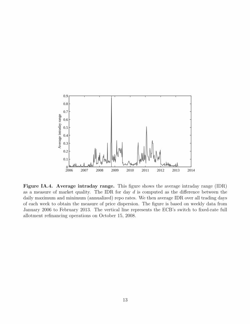
observe similar patterns when using the intraday range instead of realized volatility as a measure
of price dispersion and the illiquidity measures of Amihud (2002) and Corwin and Schultz (2012).
These measures are shown in Figures IA.4 and IA.5. Both volatility and illiquidity tend to be
higher in distressed market conditions, but fluctuate within a fairly narrow range, suggesting that
market quality for the CCP-based euro interbank repo market was not impaired. For instance, the
average volatility is only 5.2% (6.2%) before (during) the FRFA period.
11

Panel A. Average daily volatility per week
2006 2007 2008 2009 2010 2011 2012 2013 20140
0.05
0.1
0.15
0.2
0.25
Ave
rage
dai
ly v
olat
ility
Panel B. Illiquidity
2006 2007 2008 2009 2010 2011 2012 2013 20140
0.05
0.1
0.15
Illiq
uidi
ty
Figure IA.3. Volatility and illiquidity. Panel A shows the annualized average daily volatilityper week computed as the realized volatility of intraday trades. Panel B depicts Roll’s (1984)measure of the bid-ask spread as a proxy for market illiquidity. For each day d with intradaytrades indexed by i, we compute Rolld = 2
√min(0,−Cov(∆rGCP,i,∆rGCP,i−1)). Then we average
Rolld over all trading days of each week to obtain the illiquidity measure. The figures are based onweekly data from January 2006 to February 2013. The vertical line represents the ECB’s switchto fixed-rate full allotment refinancing operations on October 15, 2008.
12
2006 2007 2008 2009 2010 2011 2012 2013 20140
0.1
0.2
0.3
0.4
0.5
0.6
0.7
0.8
0.9
Ave
rage
intr
aday
ran
ge
Figure IA.4. Average intraday range. This figure shows the average intraday range (IDR)as a measure of market quality. The IDR for day d is computed as the difference between thedaily maximum and minimum (annualized) repo rates. We then average IDR over all trading daysof each week to obtain the measure of price dispersion. The figure is based on weekly data fromJanuary 2006 to February 2013. The vertical line represents the ECB’s switch to fixed-rate fullallotment refinancing operations on October 15, 2008.
13

Panel A. Illiquidity (Amihud (2002))
2006 2007 2008 2009 2010 2011 2012 2013 20140
1
2
3
4
5
6x 10
−4
Illiq
uidi
ty
Panel B. Illiquidity (Corwin and Schultz (2012))
2006 2007 2008 2009 2010 2011 2012 2013 20140
0.05
0.1
0.15
0.2
0.25
0.3
0.35
Illiq
uidi
ty
Figure IA.5. Alternative measures of market illiquidity. Panel A shows the Amihud (2002)measure of the price impact of a trade as proxy for illiquidity. For each day d with intraday tradesindexed by i = 1, . . . , I, we compute Amihudd = |log(rGCP,I) − log(rGCP,1)|/V OLGC
t . Then, weaverage Amihudd over all trading days of each week to obtain the illiquidity measure. Panel Bdepicts the Corwin and Schultz (2012) measure of the bid-ask spread as an additional proxy formarket illiquidity. The measure is based on the high and low repo rates for two consecutive days; seeEquation (14) in Corwin and Schultz (2012). We multiply both measures with the volume-weightedaverage repo rate to obtain estimates for the absolute price impact and bid-ask spread rather thanrelative values. The figures are based on weekly data from January 2006 to February 2013. Thevertical line represents the ECB’s switch to fixed-rate full allotment refinancing operations onOctober 15, 2008.
14

Appendix E. Robustness checks
Table IA.5
Regression results for term-adjusted trading volume
This table shows the results of regressing the term-adjusted repo volume on various state variables. The term-adjusted trading volume is constructed by multiplying trading volume for each repo transaction by the correspondingrepo maturity in days. Regressions are based on weekly data from January 2006 to February 2013. Column 2 showsresults for the sample prior to the introduction of fixed-rate full allotment refinancing operations at the ECB onOctober 15, 2008. Column 3 presents regression results for the sample period after this date. HAC standard errorsare shown in parentheses. The stars ∗∗∗, ∗∗, and ∗ indicate statistical significance at the 1%, 5%, and 10% level,respectively.
Prior to full allotment After full allotment
const. 4.525 0.921(5.125) (3.176)
trend 0.003 0.034 ∗ ∗∗(0.005) (0.009)
S1dt−1 −3.403 −6.960 ∗ ∗
(7.950) (3.109)ATt−1 −0.073 0.802 ∗ ∗∗
(0.165) (0.281)
V OLGC,tat−1 −0.013 −0.259 ∗ ∗
(0.234) (0.124)V OLEONIA
t−1 −0.574 −0.740 ∗ ∗(0.363) (0.321)
CISSt−1 10.459 ∗ ∗∗ 7.396 ∗ ∗∗(3.356) (2.236)
ELt−1 −20.468 −18.513 ∗ ∗∗(18.426) (6.280)
ELt−1 ∗DUMEL>300t−1 10.348 ∗ ∗
(4.734)HCRt−1 4.474
(3.800)EMCt−1 0.584 −0.708
(1.772) (2.267)
Adj. -R2 0.469 0.183
15

Table
IA.6
Regre
ssio
nre
sult
sfo
rdiff
ere
nt
risk
measu
res
Th
ista
ble
show
sth
ees
tim
ated
coeffi
cien
tsof
diff
eren
tri
skm
easu
res
wh
enre
gre
ssin
gth
ere
po
spre
ad
(St),
rep
otr
ad
ing
volu
me
(VOL1d
t),
an
dth
eav
erag
ere
po
term
(ATt)
onva
riou
sst
ate
vari
able
s.E
ach
colu
mn
corr
esp
on
ds
toa
regre
ssio
nw
ith
the
dep
end
ent
vari
ab
lesh
own
inth
efi
rst
row
.T
he
regr
essi
ons
are
the
sam
eas
inE
qu
atio
ns
(1)
to(3
)in
the
main
pap
er,
bu
tin
each
row
ad
iffer
ent
pro
xy
for
risk
isu
sed,
whic
his
indic
ate
din
the
firs
tco
lum
n.
Th
ein
tere
stra
tesp
read
s(L
IBOIS
,10ySpreadESP−GER
,an
d10y
SpreadITA−GER
)are
mea
sure
din
per
centa
ge
poin
ts.
CD
Ssp
read
san
dvo
lati
lity
(iTra
xx
andVSTOXX
)ar
em
easu
red
inp
erce
nt.
Ab
solu
teva
lues
of
targ
etbala
nce
s(T
ARGET
Germ
any
an
dTARGET
GIIPS
)are
mea
sure
din
EU
Rtr
illi
on.
Reg
ress
ion
sar
eb
ased
on
wee
kly
data
from
Janu
ary
2006
toF
ebru
ary
2013.
Colu
mn
s2
to4
show
resu
lts
for
the
sam
ple
pri
orto
the
intr
od
uct
ion
offi
xed
-rat
efu
llal
lotm
ent
refi
nan
cin
gop
erati
on
sat
the
EC
Bon
Oct
ob
er15,
2008.
Colu
mn
s5
to7
pre
sent
regre
ssio
nre
sult
sfo
rth
esa
mp
lep
erio
daf
ter
this
dat
e.H
AC
stan
dard
erro
rsare
show
nin
pare
nth
eses
.T
he
stars∗∗∗ ,∗∗
,an
d∗
ind
icate
stati
stic
al
sign
ifica
nce
at
the
1%,
5%,
and
10%
level
,re
spec
tive
ly.
Pri
or
tofu
llall
otm
ent
Aft
erfu
llall
otm
ent
S1d
tVOL1d
tATt
S1d
tVOL1d
tATt
CISSt−
10.
046
0.558∗∗
4.569∗∗∗
0.0
43
0.7
08∗∗∗
−0.0
55
(0.0
75)
(0.2
24)
(1.6
75)
(0.0
38)
(0.1
80)
(0.8
97)
LIBOISt−
1−
0.03
7∗
−0.
047
1.134
0.030
0.3
62∗∗∗
−0.6
15
(0.0
22)
(0.1
23)
(0.8
43)
(0.0
21)
(0.1
34)
(0.5
06)
iTra
xxt−
10.
055
0.236∗∗
2.138∗∗∗
0.006
0.1
18∗∗
0.2
64
(0.0
35)
(0.1
00)
(0.5
59)
(0.0
10)
(0.0
57)
(0.2
87)
TARGET
Germ
any
t−1
0.01
43.
004∗∗∗
9.515∗∗
−0.
041
1.5
33∗
2.0
65
(0.1
98)
(0.9
34)
(4.3
85)
(0.0
73)
(0.8
14)
(1.7
85)
TARGET
GIIPS
t−1
0.29
70.
203
25.
561∗∗∗
0.024
1.0
78∗∗
1.2
83
(0.3
31)
(0.9
79)
(6.6
08)
(0.0
51)
(0.5
12)
(1.3
55)
VSTOXX
t−1
0.00
00.
016∗∗∗
0.070
0.000
0.0
09∗∗
−0.0
16
(0.0
01)
(0.0
04)
(0.0
56)
(0.0
01)
(0.0
04)
(0.0
16)
10ySpreadESP−GER
t−1
0.1
000.
179
5.038∗∗∗
−0.
003
0.0
70∗∗
0.1
24
(0.0
70)
(0.2
34)
(1.4
35)
(0.0
07)
(0.0
35)
(0.1
71)
10ySpreadITA−GER
t−1
0.0
880.
295
5.713∗∗∗
0.001
0.0
73
0.0
71
(0.0
94)
(0.3
72)
(1.5
54)
(0.0
07)
(0.0
45)
(0.1
77)
16

Table
IA.7
Regre
ssio
nre
sult
sfo
rth
ehyp
oth
eti
cal
case
inw
hic
htr
aders
could
fore
cast
inte
rest
rate
sp
erf
ect
ly
Th
ista
ble
show
sth
ere
sult
sof
regr
essi
ng
the
rep
osp
read
,re
po
trad
ing
volu
me,
an
dth
eav
erage
rep
ote
rmon
vari
ou
sst
ate
vari
ab
les.
Com
pare
dto
Tab
le2
ofth
em
ain
pap
er,
the
vari
able
EM
Cis
rep
lace
dbyEM
Cperfect,
wh
ich
isco
mp
ute
das
the
diff
eren
ceb
etw
een
the
Eon
iara
teon
em
onth
inth
efu
ture
and
tod
ay’s
Eon
iara
te,
cap
turi
ng
the
hyp
oth
etic
al
case
inw
hic
htr
ad
ers
cou
ldfo
reca
stin
tere
stra
tes
per
fect
ly.
Each
colu
mn
corr
esp
on
ds
toa
regr
essi
onw
ith
the
dep
end
ent
vari
able
show
nin
the
firs
tro
w,
wh
erea
sth
eex
pla
nato
ryva
riab
les
are
show
nin
the
firs
tco
lum
n.
Reg
ress
ion
sare
bas
edon
wee
kly
dat
afr
omJan
uar
y20
06to
Feb
ruary
2013.
Colu
mns
2to
4sh
owre
sult
sfo
rth
esa
mp
lep
rior
toth
ein
trod
uct
ion
of
fixed
-rate
full
allo
tmen
tre
fin
anci
ng
oper
atio
ns
atth
eE
CB
onO
ctob
er15,
2008.
Colu
mn
s5
to7
pre
sent
regre
ssio
nre
sult
sfo
rth
esa
mp
lep
erio
daft
erth
isd
ate
.H
AC
stan
dar
der
rors
are
show
nin
par
enth
eses
.T
he
stars∗∗∗ ,∗∗
,an
d∗
ind
icate
stati
stic
al
sign
ifica
nce
at
the
1%
,5%
,an
d10%
leve
l,re
spec
tivel
y.
Pri
or
tofu
llall
otm
ent
Aft
erfu
llall
otm
ent
S1d
tVOL1d
tATt
S1d
tVOL1d
tATt
con
st.
0.6
44∗∗∗
0.366
3.440∗
0.0
75∗∗
0.188
4.898∗∗∗
(0.1
47)
(0.4
18)
(1.9
71)
(0.0
30)
(0.2
23)
(0.6
96)
tren
d0.0
02∗∗∗
0.0
05∗∗∗
(0.0
01)
(0.0
01)
S1d
t−1
−0.
157
−0.
057
−1.
429
0.574∗∗∗
0.2
58
−3.8
13∗∗∗
(0.2
50)
(0.6
55)
(3.7
23)
(0.0
70)
(0.2
72)
(1.0
63)
ATt−
1−
0.00
2−
0.032∗∗∗
0.020
−0.0
01
−0.0
31∗∗∗
0.3
09∗∗∗
(0.0
03)
(0.0
11)
(0.0
79)
(0.0
02)
(0.0
11)
(0.0
59)
VOLGC,1d
t−1
−0.
031
0.447∗∗∗
−1.
191∗
0.0
03
0.2
67∗∗∗
−0.8
94∗∗∗
(0.0
26)
(0.1
09)
(0.6
54)
(0.0
15)
(0.0
68)
(0.3
25)
VOLGC,1d
t−1∗DUM
EL>300
t−1
−0.0
38∗∗
(0.0
17)
VOLEON
IA
t−1
−0.
033
−0.0
88∗∗∗
(0.0
22)
(0.0
32)
CISSt−
10.
009
0.514∗∗
4.207∗∗
−0.0
10
0.6
42∗∗∗
−0.1
74
(0.0
52)
(0.2
12)
(1.6
23)
(0.0
33)
(0.1
69)
(0.8
28)
ELt−
1−
0.80
60.
268
−14.
361
−0.3
94∗∗∗
−0.8
35∗∗
−3.3
05
(0.7
50)
(1.5
67)
(12.1
80)
(0.1
14)
(0.4
11)
(2.6
06)
ELt−
1∗DUM
EL>300
t−1
0.3
18∗∗∗
−0.3
12
3.7
70∗
(0.0
91)
(0.3
01)
(2.2
46)
HCR
t−1
0.1
55∗
0.4
05
2.1
24
(0.0
88)
(0.4
94)
(1.4
71)
EM
Cperfect
t−1
−0.
083∗
−0.
079
−1.
038
−0.0
49
−0.2
83∗
−0.6
54
(0.0
42)
(0.0
94)
(0.8
92)
(0.0
34)
(0.1
44)
(1.0
55)
Ad
j.-R
20.
133
0.772
0.078
0.713
0.5
48
0.321
17

Table
IA.8
Regre
ssio
nre
sult
sfo
rfirs
tdiff
ere
nce
s
Th
ista
ble
show
sth
ere
sult
sof
regr
essi
ng
chan
ges
inth
ere
po
spre
ad
,ch
an
ges
inth
ere
po
trad
ing
volu
me,
an
dch
an
ges
inth
eav
erage
rep
ote
rmon
lagg
edch
ange
sin
vari
ous
stat
eva
riab
les.
Eac
hco
lum
nco
rres
pon
ds
toa
regre
ssio
nw
ith
the
dep
end
ent
vari
ab
lesh
own
inth
efi
rst
row
,w
her
eas
the
exp
lan
ator
yva
riab
les
are
show
nin
the
firs
tco
lum
n.
Reg
ress
ion
sare
base
don
wee
kly
data
from
Janu
ary
2006
toF
ebru
ary
2013.
Colu
mn
s2
to4
show
resu
lts
for
the
sam
ple
pri
orto
the
intr
od
uct
ion
of
fixed
-rate
full
all
otm
ent
refi
nan
cin
gop
erati
on
sat
the
EC
Bon
Oct
ob
er15,
2008.
Colu
mn
s5
to7
pre
sent
regr
essi
onre
sult
sfo
rth
esa
mp
lep
erio
daft
erth
isd
ate
.H
AC
stan
dard
erro
rsare
show
nin
pare
nth
eses
.T
he
stars∗∗∗ ,∗∗
,an
d∗
ind
icate
stat
isti
cal
sign
ifica
nce
atth
e1%
,5%
,an
d10
%le
vel,
resp
ecti
vely
.
Pri
or
tofu
llall
otm
ent
Aft
erfu
llall
otm
ent
∆S1d
t∆VOLGC,1d
t∆ATt
∆S1d
t∆VOLGC,1d
t∆ATt
con
st.
−0.
001
0.0
09
0.0
23
0.000
0.0
06
0.0
25
(0.0
03)
(0.0
11)
(0.0
87)
(0.0
04)
(0.0
16)
(0.0
87)
∆S1d
t−1
−0.
748∗∗∗
0.945
−1.
914
−0.0
78
0.0
85
−4.
928∗∗
(0.2
42)
(0.7
40)
(5.0
72)
(0.1
35)
(0.3
38)
(1.9
72)
∆ATt−
1−
0.00
2−
0.021∗∗∗
−0.
486∗∗∗
0.0
01
−0.
014
−0.
265∗∗∗
(0.0
02)
(0.0
07)
(0.0
53)
(0.0
01)
(0.0
10)
(0.0
49)
∆VOLGC,1d
t−1
−0.
083∗
−0.
110
−0.
225
−0.0
11
−0.
390∗∗∗
0.277
(0.0
46)
(0.1
17)
(0.9
70)
(0.0
16)
(0.0
62)
(0.3
54)
∆VOLGC,1d
t−1∗DUM
EL>300
t−1
0.0
22
(0.0
18)
∆VOLEON
IA
t−1
−0.
048
−0.
141∗∗
(0.0
33)
(0.0
58)
∆CISSt−
10.
139
0.3
54
7.3
60∗
0.1
32
0.6
44
5.6
37∗∗∗
(0.0
96)
(0.4
01)
(4.2
03)
(0.0
82)
(0.4
62)
(1.7
73)
∆ELt−
1−
0.66
50.1
50
−26.
514∗∗
−0.5
25∗∗
0.099
−10.3
85∗
(0.6
59)
(1.7
00)
(10.
932)
(0.2
06)
(1.1
57)
(5.4
62)
∆ELt−
1∗DUM
EL>300
t−1
0.3
61
−1.4
38
9.0
74
(0.2
33)
(1.8
41)
(7.8
05)
∆HCR
t−1
0.0
60
0.5
17
7.8
83
(0.1
80)
(0.7
04)
(6.4
51)
∆EM
Ct−
1−
0.01
00.4
97∗
3.648
0.022
0.1
29
−1.
581
(0.0
46)
(0.2
81)
(2.5
99)
(0.0
99)
(0.3
00)
(1.2
01)
Ad
j.-R
20.
358
0.1
14
0.3
60
0.044
0.1
93
0.1
28
18

Table
IA.9
Regre
ssio
nre
sult
sfo
rvect
or
auto
regre
ssio
nm
odel
Th
ista
ble
show
sth
ere
sult
sof
regr
essi
ng
the
rep
osp
read
,re
po
trad
ing
volu
me,
an
dth
eav
erage
rep
ote
rmon
vari
ou
sst
ate
vari
ab
les.
Com
pare
dto
Tab
le2
inth
em
ain
pap
er,
all
stat
eva
riab
les
are
incl
ud
edfo
rea
chd
epen
den
tva
riab
le.
Each
colu
mn
corr
esp
on
ds
toa
regre
ssio
nw
ith
the
dep
end
ent
vari
able
show
nin
the
firs
tro
w,
wh
erea
sth
eex
pla
nato
ryva
riable
sare
show
nin
the
firs
tco
lum
n.
Reg
ress
ion
sare
base
don
wee
kly
data
from
Janu
ary
2006
toF
ebru
ary
2013
.C
olu
mn
s2
to4
show
resu
lts
for
the
sam
ple
pri
or
toth
ein
trod
uct
ion
of
fixed
-rate
full
all
otm
ent
refi
nan
cin
gop
erati
on
sat
the
EC
Bon
Oct
ober
15,
2008
.C
olu
mn
s5
to7
pre
sent
regre
ssio
nre
sult
sfo
rth
esa
mp
lep
erio
daft
erth
isd
ate
.H
AC
stan
dard
erro
rsare
show
nin
par
enth
eses
.T
he
star
s∗∗∗ ,∗∗
,an
d∗
ind
icat
est
ati
stic
al
sign
ifica
nce
at
the
1%
,5%
,an
d10%
leve
l,re
spec
tivel
y.
Pri
or
tofu
llall
otm
ent
Aft
erfu
llall
otm
ent
S1d
tVOL1d
tATt
S1d
tVOL1d
tATt
con
st.
0.6
07∗∗∗
0.042
5.584∗
0.0
27
0.202
4.778∗∗∗
(0.0
84)
(0.3
50)
(2.9
28)
(0.0
57)
(0.2
73)
(1.5
54)
tren
d0.0
000.
003∗∗∗
−0.
003
0.000
0.0
05∗∗∗
0.004
(0.0
00)
(0.0
01)
(0.0
06)
(0.0
00)
(0.0
01)
(0.0
06)
S1d
t−1
−0.
058
0.465
−2.
820
0.603∗∗∗
0.1
95
−4.2
54∗∗
(0.1
41)
(0.5
87)
(4.9
07)
(0.0
64)
(0.3
09)
(1.7
61)
ATt−
1−
0.00
3−
0.032∗∗∗
0.003
−0.0
01
−0.0
32∗∗∗
0.2
98∗∗∗
(0.0
03)
(0.0
11)
(0.0
88)
(0.0
02)
(0.0
12)
(0.0
66)
VOLGC,1d
t−1
−0.
039∗∗
0.446∗∗∗
−1.
278∗∗
0.0
03
0.2
76∗∗∗
−0.8
25∗∗
(0.0
19)
(0.0
77)
(0.6
46)
(0.0
15)
(0.0
71)
(0.4
06)
VOLGC,1d
t−1∗DUM
EL>300
t−1
−0.0
32∗
−0.0
44
−0.6
42
(0.0
17)
(0.0
83)
(0.4
73)
VOLEON
IA
t−1
−0.
007
−0.
033
−0.
335∗
0.0
09
−0.0
85∗∗
−0.1
23
(0.0
05)
(0.0
21)
(0.1
74)
(0.0
07)
(0.0
35)
(0.2
01)
CISSt−
10.
056
0.558∗∗∗
5.983∗∗∗
0.0
19
0.7
02∗∗∗
0.4
12
(0.0
44)
(0.1
82)
(1.5
25)
(0.0
44)
(0.2
11)
(1.2
02)
ELt−
1−
0.77
7∗∗∗
0.508
−18.
002∗
−0.2
76∗∗∗
−0.8
26∗
−5.0
54∗
(0.2
94)
(1.2
22)
(10.2
09)
(0.1
03)
(0.4
95)
(2.8
23)
ELt−
1∗DUM
EL>300
t−1
0.2
41∗∗∗
−0.2
15
5.6
00∗∗
(0.0
92)
(0.4
40)
(2.5
11)
HCR
t−1
0.1
74∗∗
0.4
24
0.6
54
(0.0
86)
(0.4
15)
(2.3
67)
EM
Ct−
10.
044
0.234
−0.
157
0.042
−0.1
10
−0.6
38
(0.0
44)
(0.1
84)
(1.5
35)
(0.0
39)
(0.1
86)
(1.0
63)
Ad
j.-R
20.
080
0.774
0.089
0.711
0.5
42
0.318
19

Table IA.10
Regression results with LTRO volume
This table shows the results of regressing the repo spread, repo trading volume, and the average repo term on variousstate variables. The regressions are the same as in Table 2 of the main paper, but allowing for a separate effect ofthe 3-year LTROs by including V OLLTRO and EL, which corresponds to excess liquidity minus the outstandingvolume of the 3-year LTROs, rather than EL as explanatory variables. Each column corresponds to a regressionwith the dependent variable shown in the first row, whereas the explanatory variables are shown in the first column.Regressions are based on weekly data from October 2008 to February 2013, that is, the sample after the introductionof fixed-rate full allotment refinancing operations at the ECB. HAC standard errors are shown in parentheses. Thestars ∗∗∗, ∗∗, and ∗ indicate statistical significance at the 1%, 5%, and 10% level, respectively.
Regression results
S1dt V OL1d
t ATt
const. 0.027 0.255 4.555 ∗ ∗∗(0.033) (0.250) (0.752)
trend 0.005 ∗ ∗∗(0.001)
S1dt−1 0.660 ∗ ∗∗ 0.168 −3.402 ∗ ∗∗
(0.074) (0.262) (1.040)ATt−1 0.000 −0.032 ∗ ∗∗ 0.315 ∗ ∗∗
(0.002) (0.011) (0.059)V OL1d
t−1 −0.005 0.263 ∗ ∗∗ −0.911 ∗ ∗∗(0.015) (0.068) (0.334)
V OL1dt−1 ∗DUMEL>300
t−1 −0.012(0.017)
V OLEONIA,1dt−1 −0.088 ∗ ∗∗
(0.032)CISSt−1 0.062 0.697 ∗ ∗∗ 0.228
(0.040) (0.178) (0.971)
ELt−1 −0.227 ∗ ∗ −0.960 ∗ ∗∗ −1.870(0.092) (0.334) (1.989)
HCRt−1 0.164∗ 0.462 2.177(0.091) (0.506) (1.490)
EMCt−1 0.074 −0.136 0.022(0.057) (0.193) (0.888)
V OLLTROt−1 −0.117 ∗ ∗ −1.098 ∗ ∗∗ 0.035
(0.053) (0.236) (0.973)
Adj. -R2 0.709 0.542 0.316
20

Table IA.11
Regression results with LTRO dummy variable
This table shows the results of regressing the repo spread, repo trading volume, and the average repo term on variousstate variables. The regressions are the same as in Table 2 of the main paper, but replaces the dummy variableDUMEL>300 with DUMLTRO. Moreover, we allow for a separate effect of the 3-year LTROs by including a dummyvariable DUMLTRO that equals one after the first three year LTRO on December 21, 2011 and zero otherwise.Moreover, we interact this variable with risk. Each column corresponds to a regression with the dependent variableshown in the first row, whereas the explanatory variables are shown in the first column. Regressions are basedon weekly data from October 2008 to February 2013, that is, the sample after the introduction of fixed-rate fullallotment refinancing operations at the ECB. HAC standard errors are shown in parentheses. The stars ∗∗∗, ∗∗, and∗ indicate statistical significance at the 1%, 5%, and 10% level, respectively.
Regression results
S1dt V OL1d
t ATt
const. 0.027 0.185 5.833 ∗ ∗∗(0.040) (0.266) (0.800)
trend 0.005 ∗ ∗∗(0.001)
DUMLTRO 0.043 −0.139 −0.326(0.040) (0.201) (0.957)
S1dt−1 0.646 ∗ ∗∗ 0.174 −4.586 ∗ ∗∗
(0.086) (0.252) (1.117)ATt−1 0.000 −0.032 ∗ ∗∗ 0.274 ∗ ∗∗
(0.002) (0.011) (0.059)V OL1d
t−1 0.000 0.270 ∗ ∗∗ −0.906 ∗ ∗∗(0.014) (0.071) (0.326)
V OL1dt−1 ∗DUMLTRO
t−1 −0.038(0.023)
V OLEONIA,1dt−1 −0.085 ∗ ∗∗
(0.032)CISSt−1 0.059 0.718 ∗ ∗∗ −0.992
(0.046) (0.189) (0.957)CISSt−1 ∗DUMLTRO
t−1 −0.112 ∗ ∗ 0.015 5.291 ∗ ∗(0.055) (0.417) (2.389)
ELt−1 −0.254 ∗ ∗ −0.901 ∗ ∗ −4.316∗(0.122) (0.369) (2.315)
ELt−1 ∗DUMLTROt−1 0.205 ∗ ∗ −0.065 2.660
(0.101) (0.336) (2.281)HCRt−1 0.151 0.438 1.347
(0.093) (0.533) (1.401)EMCt−1 0.068 −0.132 −0.990
(0.064) (0.203) (0.946)
Adj. -R2 0.710 0.539 0.344
21

Appendix F. Additional figures and tables
2006 2007 2008 2009 2010 2011 2012 2013 2014
Ave
rage
term
(in
day
s)
0
5
10
15
Figure IA.6. Average repo term. This figure shows the volume-weighted average GCP term (indays) for the ECB basket. The figure is based on weekly data from January 2006 to February 2013.The vertical line represents the ECB’s switch to fixed-rate full allotment refinancing operations onOctober 15, 2008.
22

Panel A. Interest rates
2006 2007 2008 2009 2010 2011 2012 2013 2014
Inte
rest
rat
e
0
1
2
3
4
5
6
GermanyFranceItaly
Panel B. Spread over rate for GCP ECB basket
2006 2007 2008 2009 2010 2011 2012 2013 2014
Spre
ad o
ver
rate
for
GC
P E
CB
bas
ket
-1
-0.5
0
0.5
GermanyFranceItaly
Figure IA.7. Volume-weighted average repo rate for BrokerTec and MTS data. Panel Ashows the volume-weighted average repo rate for repos with German, French, and Italian govern-ment securities as collateral that are traded on BrokerTec or MTS. Panel B shows the differencebetween the interest rate for the RFR indices and the GCP ECB basket. A positive spread indi-cates that the RFR rate is higher than the GCP rate. The figures are based on weekly data fromJanuary 2006 to February 2013. The vertical line represents the ECB’s switch to fixed-rate fullallotment refinancing operations on October 15, 2008.
23

Panel A. Volume
2006 2007 2008 2009 2010 2011 2012 2013 2014
Vol
ume
(in
EU
R b
illio
ns)
0
20
40
60
80
100
120
140
160
180
200
GermanyFranceItaly
Panel B. Share of different countries
2006 2007 2008 2009 2010 2011 2012 2013 2014
Shar
e
0
0.1
0.2
0.3
0.4
0.5
0.6
0.7
0.8
0.9
1
GermanyFranceItaly
Figure IA.8. Volume on BrokerTec and MTS. Panel A presents the average daily tradingvolume for repos trading on BrokerTec and MTS that are part of the RFR indices. The correspond-ing shares of total trading volume are plotted in Panel B. The figures are based on weekly datafrom January 2006 to February 2013. The vertical line represents the ECB’s switch to fixed-ratefull allotment refinancing operations on October 15, 2008.
24

References
Amihud, Yakov (2002), Illiquidity and Stock Returns: Cross-section and Time-series Effects, Jour-
nal of Financial Markets 5, 31–56.
Corwin, Shane A., and Paul Schultz (2012), A Simple Way to Estimate Bid-Ask Spreads from
Daily High and Low Prices, Journal of Finance 67, 719–760.
Eurex Repo (2013), GC Pooling Basket Definition, February 2013, Eurex Repo, http://www.
eurexrepo.com/repo-en/products/gcpooling/.
O’Hara, Maureen, and Mao Ye (2011), Is Market Fragmentation Harming Market Quality?, Jour-
nal of Financial Economics 100, 459–474.
Roll, Richard (1984), A Simple Implicit Measure of the Effective Bid-Ask Spread in an Efficient
Market, Journal of Finance 39, 1127–1139.
25


