
THE EFFECT OF STIRRED MILL OPERATION ON PARTICLES
BREAKAGE MECHANISM AND THEIR MORPHOLOGICAL
FEATURES
by
REEM ADEL ROUFAIL
B.Sc., The American University in Cairo, 1992
M.Sc., The American University in Cairo, 1997
A THESIS SUBMITTED IN PARTIAL FULFILLMENT OF
THE REQUIREMENTS FOR THE DEGREE OF
DOCTOR OF PHILOSOPHY
in
THE FACULTY OF GRADUATE STUDIES
(Mining Engineering)
THE UNIVERSITY OF BRITISH COLUMBIA
(Vancouver)
October 2011
© Reem Adel Roufail, 2011

ii
Abstract
Stirred milling is a grinding tool that is used extensively for mineral liberation, in order to
achieve successful downstream processing such as flotation or leaching. The focus of this
research is to understand the effect of different operating parameters on particle breakage
mechanism. Operating parameters could be summarized as stress intensity on the particles which
are varied by changing the mill’s agitator speed, and different ground material properties such as
extreme hard/low density minerals like quartz versus soft/high density minerals like galena.
Grinding performance is assessed by analysing particle size reduction and energy consumption.
Breakage mechanism is evaluated using the state of the art morphological analysis and liberation.
Finally, theoretical evaluation of particles flow, types of forces and energy distribution across the
mill are investigated using Discrete Element Modelling (DEM).
It is observed that breakage mechanisms are affected by the type of mineral and stress intensities
(agitator speed) in the mill. For example, galena, the soft/high density mineral, reaches its
grinding limit very fast at high agitator speed and specific energy consumption increases
exponentially with the increase of the agitator speed. On the other hand, for quartz, the hard/low
density mineral, the breakage rate is very slow at low agitator speed and the specific energy
consumption increases linearly with the increase of the agitator speed. Fracture mechanism of the
particles is also function of the agitator speed and type of mineral. At high agitator speed, galena
fractures mostly along the grain boundaries, whereas quartz breaks across the grains, which is
abrasion. The morphology observation is confirmed by the DEM model, which conveyed that at
higher agitator speed, the normal forces were higher than tangential forces on the galena particles
compared to the ceramic grinding media particles.
The core of this research is the morphology analysis, which is a novel approach to studying
particle breakage mechanisms. More work is recommended in the field of morphology with other
types of minerals to confirm the findings of this research. 3D liberation analysis was introduced
in this research; a correlation to the conventional liberation methodology would be a major
addition to the industry.

iii
Preface
The research results presented in this thesis represent work conducted by the author with input
and advice from the supervisory committee.
Thus far the research has generated two publications. The first publication titled ―Mineral
Liberation and Particle Breakage in Stirred Mills‖ was presented at the 43rd
Conference of
Metallurgists in Sudbury in 2009. It was then re-published by the Canadian Metallurgical
Quarterly (Vol. 49, No4, pp 419-428, 2010). This publication was coauthored by Professor B.
Klein. I was responsible for developing the methodology to analyse the morphological features
and their parameters from Scanning Electron Microscope images. I was responsible for
developing the concepts and writing the paper, with advice of the coauthor.
The second publication titled, ―Effect of Grinding Operation and Product Morphology in Stirred
Mill‖ was coauthored by B. Klein and R. Blaskovich and was presented and published at the
43rd Annual Meeting of the Canadian Mineral Processor in Ottawa, 2011. I was responsible for
performing the experiments, defining the morphological features to be analysed, compiling the
data and writing the publication. B. Klein advised on and reviewed this publication and R.
Blaskovich acquired the SEM images and generated the fundamental data for analysis. The
results presented in the publication were included in chapters 2, 3 and 4 of this document.

iv
Table of Contents
Abstract ..................................................................................................................................... ii
Preface ...................................................................................................................................... iii
Table of Contents ...................................................................................................................... iv
List of Tables .......................................................................................................................... viii
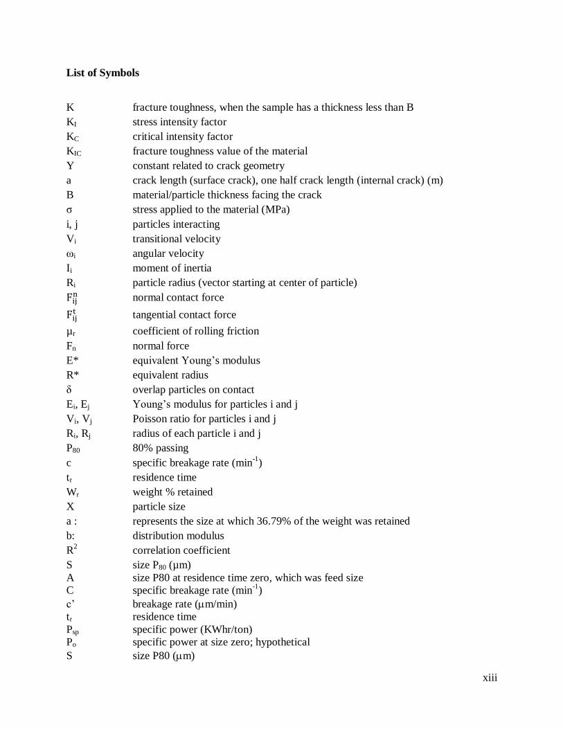
List of Symbols ....................................................................................................................... xiii
Acknowledgments ....................................................................................................................xvi
Dedication .............................................................................................................................. xvii
1. Introduction .........................................................................................................................1
1.1 Stirred Mills ..................................................................................................................1
1.2 Research Objective .......................................................................................................4
1.3 Thesis Outline ...............................................................................................................5
2. Literature Review ................................................................................................................7
2.1 Mill Operation and Particle Size Distribution ................................................................7
2.2 Failure Analysis – Brittle and Fatigue Fractures ............................................................9
2.3 Morphology ................................................................................................................ 14
2.3.1 Morphological Features of Fractured Surfaces ..................................................... 14
2.3.2 Morphological Features and Comminution ........................................................... 17
2.4 Computer Model and Mill Simulation ......................................................................... 20
2.4.1 Power Model ....................................................................................................... 25
2.5 Conclusion .................................................................................................................. 26
3. Grinding Studies ................................................................................................................ 28
3.1 Introduction ................................................................................................................ 28
3.2 Grinding Test Material ................................................................................................ 28
3.3 Procedures .................................................................................................................. 30
3.3.1 Material Preparation Procedure ............................................................................ 31
3.3.2 Grinding Procedure .............................................................................................. 33
3.3.3 Particle Size Analysis Procedure .......................................................................... 35
3.3.4 Preparation of Test Products ................................................................................ 36
3.4 Grinding Results ......................................................................................................... 38
3.4.1 Particle Size Distribution ..................................................................................... 38
3.4.2 Breakage Rate ...................................................................................................... 47

v
3.4.2.1 Initial Breakage Rate..................................................................................... 54
3.4.2.2 Average Breakage Rate ................................................................................. 55
3.4.3 Energy Consumption............................................................................................ 56
3.4.4 Effective Energy .................................................................................................. 62
3.4.5 Specific Breakage Energy .................................................................................... 65
3.5 Conclusion .................................................................................................................. 66
4. Morphology and Liberation ............................................................................................... 69
4.1 Introduction ................................................................................................................ 69
4.1.1 Morphology Definition ........................................................................................ 69
4.1.2 Morphology Evaluation ....................................................................................... 69
4.1.3 Sample Description for Morphology .................................................................... 71
4.2 Clemex Method .......................................................................................................... 72
4.3 Manual Point Counting Method .................................................................................. 74
4.3.1 Point Counting Sensitivity Analysis ..................................................................... 76
4.4 Liberation Methodology .............................................................................................. 76
4.5 Morphology and Liberation Results ............................................................................ 77
4.5.1 Manual Point Counting Results ............................................................................ 78
4.5.2 Pearson’s Correlation ........................................................................................... 79
4.5.3 Stacked Charts Analysis ....................................................................................... 90
4.5.4 Shattered Particles Feature ................................................................................. 104
4.5.5 Automated Quantitative Morphological Analysis ............................................... 105
4.5.6 Liberation Analysis Results ................................................................................ 110
4.5.7 Liberation versus Agitator Speed ....................................................................... 111
4.5.8 Particle Mount versus Polished Samples ............................................................ 117
4.6 Conclusion ................................................................................................................ 120
5. Computer Modeling and Simulation of Stirred Mill ......................................................... 123
5.1 EDEM Software ........................................................................................................ 125
5.2 DEM Simulation Limitations .................................................................................... 129
5.3 IsaMill Model Geometry ........................................................................................... 131
5.3.1 Number of Particles ........................................................................................... 134
5.3.2 Triangular versus Circular Discs ........................................................................ 135
5.3.3 Effect of Drag Forces ......................................................................................... 138
5.3.4 Material Properties ............................................................................................. 144

vi
5.3.5 Model Parameters .............................................................................................. 147
5.3.5.1 Fixed Parameters ........................................................................................ 147
5.3.5.2 Variable Parameters .................................................................................... 149
5.4 Computer Model Results ........................................................................................... 150
5.4.1 Media Particles Runs ......................................................................................... 150
5.4.1.1 Particle Distribution .................................................................................... 150
5.4.1.2 Energy Distribution ..................................................................................... 153
5.4.1.3 Forces Distribution ..................................................................................... 159
5.4.1.4 Average Force Distribution ......................................................................... 160
5.4.2 Galena and Media Particles Runs ....................................................................... 166
5.4.2.1 Particle Distribution .................................................................................... 166
5.4.2.2 Maximum Forces Distribution .................................................................... 170
5.4.2.3 Average Force Distribution ......................................................................... 171
5.5 Conclusion ................................................................................................................ 172
6. Conclusions and Recommendations ................................................................................. 175
6.1 Conclusions .............................................................................................................. 175
6.1.2 Experimental Work ............................................................................................ 176
6.1.3 Morphology ....................................................................................................... 178
6.1.4 Computer Model ................................................................................................ 180
6.2 Recommendations ..................................................................................................... 183
6.2.1 Experimental and Morphology ........................................................................... 183
6.2.2 Computer Modeling ........................................................................................... 184
References .............................................................................................................................. 185
Appendix A: Experimental Data...................................................................................................... 199
Appendix A1: MSDS Sheets ............................................................................................ 199
Appendix A2: Assay Analysis .......................................................................................... 213
Appendix A3: Measured Specific Gravity, SG ................................................................. 214
Appendix A4: Experimental Data ..................................................................................... 215
Appendix A5: Cyclone Correlation Factor ........................................................................ 226
Appendix B: Experimental Results ................................................................................................. 227
Appendix B1: Mass of Solids Calculations Based on Volume Percent .............................. 227
Appendix B2: Rosin Rammler Fit and Parameters ............................................................ 228

vii
Appendix B3: Correlation between Measured and Calculated P80 .................................... 239
Appendix B4: Energy Breakage vs. Particle Size P80 (m) .............................................. 243
Appendix C: Morphology ................................................................................................................ 245
Appendix C1: Manual Point Counting Sub-Routine ......................................................... 245
Appendix C2: Snap Shot of the Manual Point Counting Screen ........................................ 246
Appendix C3: Manual Point Counting Sensitivity Analysis .............................................. 247
Appendix C4: Clemex Routine ......................................................................................... 248
Appendix C5: Morphology Point Counting Data .............................................................. 250
Appendix C6: List of Morphology Samples ...................................................................... 265

viii
List of Tables
Table 3-1: Properties of Material Tested and Percent Solid by Mass ...................................................... 30
Table 3-2: Percent Solids by Volume and Weight for the Experimental Samples Tested......................... 33
Table 3-3: Morphology Sample Size Fractions and Geometric Mean Size .............................................. 37
Table 3-4: Size Distribution of the Samples as Received ........................................................................ 39
Table 3-5: R-Squared Values for Linear and Exponential Data Fit ......................................................... 52
Table 3-6: Initial and Average Breakage at Different Agitator Speed ..................................................... 54
Table 3-7: R2 Values for Specific Energy vs. Size Reduction Using Power and Exponential Equations ... 57
Table 3-8: Specific Breakage Energy (kJ/m) ........................................................................................ 66
Table 4-1: Morphology Roughness Level Definitions and Illustration .................................................... 75
Table 4-2: Breakage Mode versus Roughness Level .............................................................................. 78
Table 4-3: Morphological Statistical Analysis of Galena Concentrate Sample ..................................... 108
Table 4-4: Morphological Statistical Analysis of Quartz ...................................................................... 109
Table 4-5: Morphological Statistical Analysis of Mixed Quartz and Galena Concentrate Sample ......... 110
Table 4-6: Feed Sample – Difference in Distribution Between Polished and Particle Mount Samples ... 119
Table 4-7: Lead-Zinc Ore Sample 1500-P1 Sample – Difference in Distribution Between Polished and
Particle Mount Samples ....................................................................................................................... 119
Table 4-8: Lead-zinc ore sample 1500-P2 Sample – Difference in Distribution between Polished and
Particle Mount Samples ....................................................................................................................... 119
Table 4-9: Lead-zinc ore sample 1500-P3 Sample – Difference in Distribution between Polished and Particle Mount Samples ....................................................................................................................... 119
Table 5-1: Benchmark Material Properties ........................................................................................... 144
Table 5-2: Effect of Material Properties on Run Time, Forces and Energy Efficiency .......................... 147
Table 5-3: Material Properties - Fixed Parameters ................................................................................ 148
Table 5-4: Particles and Mill Component Interactions .......................................................................... 149
Table 5-5 : Maximum Normal and Tangential Forces .......................................................................... 160
Table 5-6: Normal Forces Distribution Across the Mill at 1000, 1500 and 2000 rpm Agitator Speed .... 165
Table 5-7: Mixed Media and Galena Particles Distribution at 1500 rpm ............................................... 169
Table 5-8: Mixed Media and Galena Particles Distribution at 2000 rpm ............................................... 170
Table 5-9: Maximum Normal and Tangential Forces Distribution ........................................................ 171
Table A4-1: Quartz Experimental Data at 1000 rpm............................................................................. 215
Table A4-2: Quartz Experimental Data at 1500 rpm............................................................................. 216
Table A4-3: Quartz Experimental Data at 2000 rpm............................................................................. 217
Table A4-4: Galena Concentrate Experimental Data at 1000 rpm ......................................................... 218

ix
Table A4-5: Galena Concentrate Experimental Data 1500 rpm ............................................................ 219
Table A4-6: Galena Concentrate Experimental Data at 2000 rpm ......................................................... 220
Table A4-7: Mix Quartz and Galena Concentrate Experimental Data at 1000 rpm ................................ 221
Table A4-8: Mix Quartz and Galena Concentrate Experimental Data at 2000 rpm ................................ 222
Table A4-9: Lead-Zinc Ore Experimental Data at 1000 rpm ................................................................ 223
Table A4-10: Lead-Zinc Ore Experimental Data at 1500 rpm .............................................................. 224
Table A4-11: Lead-Zinc Ore Experimental Data at 2000 rpm .............................................................. 225
Table C5-66-12C: Morphology Counts for Mixed quartz and galena Concentrate Sample (Quartz +
Galena Counts), ................................................................................................................................... 261

x
List of Figures
Figure 1-1: Reported Specific Energy per Mill Type, (Wang and Forssberg, 2007) .................................. 2
Figure 1-2: Verti Mill and SMD Mill, (Metso, 2010 [Brochure]) .............................................................. 3
Figure 1-3: IsaMill, (Gao, and Holmes, 2007) .......................................................................................... 3
Figure 2-1: Fracture Toughness Versus Material Thickness; After Farag (1989)..................................... 11
Figure 2-2: Fracture Toughness of Ductile and Brittle Material .............................................................. 11
Figure 2-3: (a) Typical Particle Shapes; (b) Perfect Circle Particle ......................................................... 13
Figure 2-4: Schematic Diagram Subjected to Compressive Force P, a) flaw inclined at angle with
respect to loading axis, b) flaw parallel to loading axis =0); After Tromans and Meech (2001).......13
Figure 2-5: Cleavage in a Low Carbon Steel Impact Fractured at Liquid Nitrogen Temperature. ............ 15
Figure 2-6: Fatigue Striation in a Low Carbon Steel Fractured Sample (Zone II). ................................... 16
Figure 2-7: Intergranular Fracture and Grain Boundary Separation for Low Alloy Steel. ........................ 16
Figure 2-8: SEM Image - 53 m Fraction; (a) BM; (b) HPGR. ............................................................... 19
Figure 2-9: SEM Image of Dense Packed Sand Grain Subjected ............................................................ 19
Figure 2-10: (a) Ball Mill, (b) Rod Mill, (c) SEM Micrograph of Ball Mill, .......................................... 19
Figure 2-11: Morphology of Gold Particles Generated by (a) Hammer Milling, (b) Disc Milling, ........... 20
Figure 3-1: Sample Preparation Flow Diagram ...................................................................................... 32
Figure 3-2: Schematic Diagram of Experimental Flow ........................................................................... 35
Figure 3-3: Correlation Coefficient versus Size Reduction ..................................................................... 40
Figure 3-4: Correlation Coefficient versus Modulus of Distribution ....................................................... 40
Figure 3-5: Rosin Rammler Modulus of Distribution versus Size Reduction .......................................... 41
Figure 3-6: Quartz Passing Percent for (a) 1000, (b) 1500 and (c) 2000 rpm ........................................... 43
Figure 3-7: Galena Concentrate Passing Percent for (a) 1000, (b) 1500 and (c) 2000 rpm ....................... 44
Figure 3-8: Mixed Quartz and Galena Sample Passing Percent for ......................................................... 45
Figure 3-9: Lead-Zinc Ore Sample Passing Percent for (a) 1000, (b) 1500 and (c) 2000 rpm .................. 46
Figure 3-10: Quartz (a) Linear and (b) Linearized Exponential Fitting Data ........................................... 48
Figure 3-11: Galena Concentrate (a) Linear and (b) Linearized Exponential Fitting Data ....................... 49
Figure 3-12: Mixed Quartz and Galena Sample (a) Linear and ............................................................... 50
Figure 3-13: Lead-Zinc Ore Sample (a) Linear and ................................................................................ 51
Figure 3-14: Correlation Between Measured and Calculated P80 for ...................................................... 53
Figure 3-15: Quartz Signature Plot – (a) Exponential and (b) Power Fit ................................................. 58
Figure 3-16: Galena Concentrate Signature Plot – (a) Exponential and (b) Power Fit ............................. 59
Figure 3-17: Mixed Quartz and Galena Sample Signature Plot ............................................................... 60
Figure 3-18: Lead-Zinc Ore Sample Signature Plot – (a) Exponential and (b) Power Fit ......................... 61

xi
Figure 3-19: Grinding Effective Energy for (a) Quartz, (b) Galena Concentrate, .................................... 64
Figure 4-1 Particle Perimeter and Hull Perimeter ................................................................................... 70
Figure 4-2: (a) Particle ID 39 Roughness value was 0.9; ........................................................................ 73
Figure 4-3: Pearson’s Time Correlation vs. Roughness Level Count ...................................................... 81
Figure 4-4: Pearson’s Time Correlation and Roughness Level Count for Quartz, ................................... 83
Figure 4-5: Pearson’s Time Correlation and Roughness Level Count for Quartz in................................. 85
Figure 4-6: Pearson’s Time Correlation and Roughness Level Count for Galena in ................................ 86
Figure 4-7: Pearson’s Time Correlation and Roughness Level Count for Cumulative ............................. 87
Figure 4-8: Pearson’s Time Correlation and Roughness Level Count for Lead-Zinc Ore Sample ............ 89
Figure 4-9: Quartz Stacked Chart of Cumulative Roughness Percent Point Count vs. Grinding Passes
1000rpm, (b) 1500rpm, (c) 2000rpm ...................................................................................................... 94
Figure 4-10: Roughness Trend of Quartz for (a) Coarse, (b) Medium (c) Fine Fractions ......................... 95
Figure 4-11: Galena Stacked Chart of Cumulative Roughness Percent Point Count vs. Grinding Passes
1000rpm, (b) 1500 rpm, (c) 2000rpm ..................................................................................................... 96
Figure 4-12: Roughness Trend of Galena Concentrate for (a) Coarse, (b) Medium (c) Fine Fractions ..... 97
Figure 4-13: Mixed Quartz and Galena Sample Stacked Chart of Cumulative Roughness Percent Point Count vs. Grinding Passes (a) 1000rpm, (b) 2000rpm ............................................................................ 98
Figure 4-14: Roughness Trend of Mixed Quartz and Galena Concentrate ............................................... 99
Figure 4-15: Lead-Zinc Ore Sample Stacked Chart of Cumulative Roughness Percent Point Count vs. Grinding Passes (a) 1000rpm, (b) 1500rpm, (c) 2000rpm ..................................................................... 100
Figure 4-16: Roughness Trend of Lead-Zinc Ore for (a) Coarse, (b) Medium (c) Fine Fractions........... 101
Figure 4-17: Overall Roughness Trend for Quartz Sample ................................................................... 102
Figure 4-18: Overall Roughness Trend for Galena Concentrate Sample ............................................... 102
Figure 4-19: Overall Roughness Trend for the Mixed Quartz and Galena Concentrate Sample ............. 103
Figure 4-20: Overall Roughness Trend for Lead – Zinc Ore Sample.................................................... 103
Figure 4-21: Individual Quartz Particles Broken, Shattered .................................................................. 105
Figure 4-22: Individual Galena Particles Broken, Shattered ................................................................. 105
Figure 4-23: Feed Liberation ............................................................................................................... 111
Figure 4-24: Lead-Zinc Ore Sample 1000 rpm - Pass1 Liberation ........................................................ 112
Figure 4-25: Lead-Zinc Ore Sample 1500 rpm - Pass1 Liberation ........................................................ 113
Figure 4-26: Lead-Zinc Ore Sample 2000 rpm - Pass1 Liberation ........................................................ 114
Figure 5-1: Schematic Diagram of Hertz Mindlin Contact Model, EDEM Training Manual, 2009 ........ 126
Figure 5-2: Schematic Diagram of Circular Agitator, Dimensions were mm ......................................... 132
Figure 5-3: Schematic Diagram of Triangular Discs Agitator ............................................................... 132
Figure 5-4: Cross Section of Particles Factory Surrounding 3 Discs ..................................................... 133
Figure 5-5: Initial Setting of the Particles in the 3 Sections at Time Zero .............................................. 135

xii
Figure 5-6: Particle Distribution in 3 Sections for Circular and Triangular Discs .................................. 137
Figure 5-7: Fluid Flow Effect with No Drag Flow at 1500 rpm Agitator Speed .................................... 140
Figure 5-8: Drag Flow Force Effect on Particle Distribution Across the Mill ........................................ 142
Figure 5-9: Particle Distribution Across the Mill: ................................................................................. 143
Figure 5-10: Particle Distribution vs. Simulation Time ........................................................................ 152
Figure 5-11: Output vs. Input Energies for Media Runs ....................................................................... 154
Figure 5-12: Media Effective Energy Ratio vs. Simulation Time .......................................................... 156
Figure 5-13: Torque vs. Simulation Time............................................................................................. 158
Figure 5-14: Instantaneous Energy vs. Time Simulation, a) Input Energy, b) Output Energy ................ 158
Figure 5-15: Mill Cross Section .......................................................................................................... 161
Figure 5-16: (a) Normal and (b) Tangential Forces Distribution in Section A-A for 1000 rpm run ........ 162
Figure 5-17: (a) Normal and (b) Tangential Forces Distribution in Section B-B for 1000 rpm .............. 163
Figure 5-18: Number of Particles Distribution Across the Mill: ............................................................ 167
Figure 5-19: Initial Particle Distribution at Time Zero: (a) Radial Direction, section B-B; (b) Linear
Direction, section A-A, (c) Isometric corss section............................................................................... 168
Figure 5-20: Normal Forces Distribution at 1500 rpm (a) Section A-A; (b) Section B-B ...................... 172
Figure 5-21: Normal Forces Distribution at 2000 rpm (a) Section A-A; (b) Section B-B ...................... 172
xiii
List of Symbols
K fracture toughness, when the sample has a thickness less than B
KI stress intensity factor
KC critical intensity factor
KIC fracture toughness value of the material
Y constant related to crack geometry
a crack length (surface crack), one half crack length (internal crack) (m)
B material/particle thickness facing the crack
σ stress applied to the material (MPa)
i, j particles interacting
Vi transitional velocity
ωi angular velocity
Ii moment of inertia
Ri particle radius (vector starting at center of particle)
normal contact force
tangential contact force
µr coefficient of rolling friction
Fn normal force
E* equivalent Young’s modulus
R* equivalent radius
δ overlap particles on contact
Ei, Ej Young’s modulus for particles i and j
Vi, Vj Poisson ratio for particles i and j
Ri, Rj radius of each particle i and j
P80 80% passing
c specific breakage rate (min-1
)
tr residence time
Wr weight % retained
X particle size
a : represents the size at which 36.79% of the weight was retained
b: distribution modulus
R2 correlation coefficient
S size P80 (µm)
A size P80 at residence time zero, which was feed size
C specific breakage rate (min-1
)
c’ breakage rate (m/min)
tr residence time
Psp specific power (KWhr/ton)
Po specific power at size zero; hypothetical
S size P80 (m)

xiv
D specific power per size reduction
Xi residence time
Yi number of particles counted per degree of roughness
X, Y mean values for residence time and number of particles
L length
W width
A area
P perimeter
HP hull perimeter
AR aspect ratio
S sphericity
Vs settling velocity
g gravity
dp particle diameter
ρp particle density
ρw water density
viscosity
SEn surface energy per unit mass
Fr surface roughness
surface energy (1/2 crack energy)
Df particle final diameter
Di particle initial diameter
Fn normal force
Y* equivalent Young’s modulus
R* equivalent radius
δn normal overlay
normal damping forces
M* equivalent mass
relative normal velocity
β , Sn normal stiffness
e coefficient of restitution
Ft tangential force
G* equivalent shear modulus
tangential damping force
St tangential stiffness
relative tangential velocity
i rolling friction
µr coefficient of rolling friction
Ri distance of contact point from object center mass
ωi angular velocity at contact point

xv
Ks linear spring stiffness
C dashpot coefficient
δn overlap
overlap velocity
E* equivalent Modulus of elasticity
rpm revolution per minute
EI input energy
T torque
t time
PSD particle size distribution
SEM scanning electron microscope
BM ball mill
HPGR high pressure grinding roll
DEM discrete element modeling method
CFD computer fluid dynamics
PEPT positron emission particles tomography
MSDS material safety data sheet
SG specific gravity
HP hull perimeter
MLA mineral liberation analysis
CAD computer aided design
CFD computational fluid dynamics
API application programming interface

xvi
Acknowledgments
I would like to express my gratitude to the following people who without them, this work would
have been impossible to achieve.
First, I would like to thank professor, Bern Klein for his support and guidance throughout this
research. I have immensely learned from your knowledge in the field of comminution and
mineral processing and gave me the freedom and confidence to try and learn new things.
I would like to extend my thankfulness to my co-advisors, professor, Peter Radziszewski for his
valuable support and technical advice in the modeling segment of this work. Your patience and
advice was highly appreciated. Also Dr. Andy Stradling, my industrial advisor and committee
member, I really appreciate your guidance and assistance that helped me to stay on track.
Professor, Marek Pawlik, committee member, your input added depth and value to my work,
thank you.
I would also like to thank Teck Cominco Ltd., ART staff for their enthusiastic support in
capturing the SEM images, Clemex data and their technical input.
I am also grateful for the support of G&T Metallurgical Services Ltd. and High Way Technical
Engineering Services Ltd. for allowing me to use their labs for sample preparation.
I would like to thank the mining engineering department’s staff and my colleagues for all the
support they’ve given me throughout the experimental process.
I can’t forget my family, especially my beloved husband and lovely children who were holding
on and gave me an enormous tangible and emotional support all through the 5 years. I couldn’t
have done it without you.
Finally, the first man in my life, my father, who believed in me, more than I believed in myself,
wished you were here to witness this.

xvii
Dedication
To My Family

1
1. Introduction
Ultra fine grinding and stirred mills are widely considered in mining operations since the
mineralogical complexity of the available ore bodies is increasing. In many cases, particles need
to be ground to 10m to liberate minerals. Over the past couple decades studies were performed
to investigate the relationship between energy, stress intensity and product particle size (Blecher
et al., 1996). Several studies focused on mill design and/or stress intensity distribution in the
grinding mill (Kwade et al., 1996; Jie et al., 1996; Kwade, 1999a). Other studies considered the
effect of the mechanical properties of the grinding media and ground material on the
comminution process (Peukert, 2004; Becker et al., 2001; Kwade and Schwedes, 2002)
1.1 Stirred Mills
Grinding is the largest energy consuming operation in mineral processing. About 50% of the
energy consumed in mining operation is consumed in comminution operation (Botin, 2009).
High speed stirred milling is the only technology that is employed in metal mining to grind
particles down to ultrafine particle sizes (below 10m). The ability to grind to this particle size
range relates to the power intensity in stirred mills which is about 300 kW/m3, compared to ball
mills and tower mills that are 20 kW/m3 and 40 kW/m
3, respectively (Pease et al., 2006). Despite
the high power intensity, the overall power consumption of high speed stirred mills is lower due
to their high specific throughput reflected by short retention times. Figure 1-1 compares the
specific energy input and particle size reduction for different types of mills. Stirred mills have
the highest specific energy input, but are the only mills that have the capability to grind particles
below 5 microns.

2
Figure 1-1: Reported Specific Energy per Mill Type, (Wang and Forssberg, 2007)
The main types of stirred mills used in the mining industry are the IsaMill, the Stirred Media
Detritor (SMD) and the Verti mill. The IsaMill and SMD are high speed mills and the Verti mill
is a low speed mill. The IsaMill is horizontally oriented and the latter two mills are vertically
oriented. Another difference is the agitator type. The SMD uses pin agitator; the Verti mill uses a
helical agitator (Figure 1-2) and the IsaMill employs discs (Figure 1-3). The power intensity of
the IsaMill is 400 kW/m3 compared to 150 kW/m
3 of the SMD mill, 19 kW/m
3 of the ball mill
and 4 kW/m3
for the Verti-Tower mill (Xstrata Technology 2010).

3
Figure 1-2: Verti Mill and SMD Mill, (Metso, 2010 [Brochure])
Figure 1-3: IsaMill, (Gao, and Holmes, 2007)
Another difference between high speed mills and both the Verti mills and ball mills is that high
speed mills are typically run in open circuit (no size classification). Over the past few decades
research studies, such as those by Kwade and Becker (2001), were performed to relate different
4
forms of energy (input energy, specific energy, volume / mass specific energies), stress intensity
and the final product particle size. Other studies focused on mill design and/or stress intensity
distribution in the grinding mill (Becker et al., 1996, Kwade, 1999, 1996, Blecher et al, 1996,
Partyka and Yan, 2007, Stender et al., 2004). The mechanical properties of the grinding media
and ground material on the comminution process were also considered (Peukert, 2004).
Stress intensity and energy in stirred mills were extensively researched. Attrition was considered
to be the main breakage mechanism; however the actual breakage mechanisms encountered in
the stirred mills are not well understood.
1.2 Research Objective
The primary objective of this research is to gain an understanding of how operating parameters
affect breakage mechanism. The objective is achieved via theoretical and experimental work.
The secondary objective is to develop an understanding of the grinding mechanism of stirred
mills via studying the state of the art researches performed on stirred mills using different tools
including particle breakage analysis, morphology and computer modeling techniques.
Specific objectives of the research were:
To study the effect of different operating conditions and different material properties on
grinding performance via analysing particle size reduction and energy consumption.
To develop an understanding of the effect of breakage mechanism under varying mill
operating conditions as well as mechanical material properties on particle morphology
and liberation.
To create a computer model that simulates particle flow, forces and energy distribution
across the mill under different operating conditions.

5
1.3 Thesis Outline
The state of the art literature is reviewed in chapter 2. The published literature reviews
information about stirred mill operation and summarises the topics of failure analysis, types of
fracture, morphology analysis, Discrete Element Modeling (DEM) and simulation.
The results of the research are presented in three chapters, relating to grinding studies,
morphological analysis and DEM.
In chapter 3, test procedures and results of grinding studies are presented. Criteria for selecting
material are reviewed. Material preparation and grinding procedures are outlined. Grinding
results such as particle size distribution, breakage rates, Rosin Rammler fit and energy
consumptions are summarized.
In chapter 4, morphology definitions and analysis procedures are validated. Morphological
analysis procedures are performed via manual point counting and pre-programmed image
analysis software. The effect of residence time on the degree of roughness is analysed both
statistically and cumulatively. Manual point count data are statistically analysed using Pearson’s
Correlation, and cumulatively analyzed using stacked charts and degree of roughness trends.
Whereas, the pre-programmed data, acquired via image analysis software, are analysed using
general descriptive statistics. Liberation analysis of a lead-zinc ore sample, at three agitator
speeds, is also addressed in chapter 4.
In chapter 5, the discrete element modeling technique (DEM), the software utilizing (EDEM),
the equations employed and the operating parameters are summarized. The simulation runs are
analysed across the mill based on three criteria; number of particles, energy distribution and
types and magnitude of forces the particles generated.

6
Finally chapter 6 presents the main findings and conclusions of the research. Recommendations
for future research are also presented in the same chapter.

7
2. Literature Review
The Literature review covers three main areas, the relationship between mill operation and size
reduction, morphology analysis and discrete element modeling (DEM).
Despite all the researches and studies performed on stirred mills, the operation and performance
of these mills were only empirically understood. Particle breakage mechanism versus operating
conditions of the mill was rarely studied. In this research, a comprehensive understanding of the
fundamental mill operation and its products (ground particles) were explored, focusing on
particle breakage mechanisms.
The use of morphological analysis to understand the breakage mode of the particles under
different grinding mechanisms represents a novel approach. The literature was reviewed to
summarize the relationship between breakage mode and surface texture (morphology features).
In order to simulate breakage in stirred mills, the modeling should accurately simulate particle
motion and forces in the mill. However, it was recognised that limitations to modeling existed,
which leads to oversimplification of the system. A summary of computer modeling (DEM) of
stirred mills was included in this chapter.
2.1 Mill Operation and Particle Size Distribution
Stirred mills, by definition, are mills that stir particles which are usually in slurry form and need
to be ground. Grinding media could be natural sand, steel slag or ceramic beads. The stirred mills
are classified according to their orientation i.e. vertical or horizontal. Examples of vertical mills
are tower mills, pin mills and the stirred media detritor (SMD), whereas the IsaMill is a
horizontal mill. A vast number of researchers (Gao and Forssberg, 1993, Blecher et al., 1996,
Kwade et al, 1996, Zheng, et al., 1996 , Gao et. al, 1996, Varinot et. al, 1999, Kwade, 1999,

8
2004, Wang and Forssberg, 2000, Becker et al., 2001, Kwade and Schwededs, 2002, Jankovic,
2003, Stender, et al., 2004, Yue, and Klein, 2005, Parry, 2006, Gao and Holmes, 2007, Shi, et al.,
2009, Ye, et al., 2010, Pease, et al., 2010, Vizcarra et al., 2010, Celep et al., 2011, and others)
investigated different types of stirred mills operation, stress energy distribution, stress types,
energy consumption, breakage kinetics, mineral liberation, product size distribution, mineral
flotation performance and other parameters.
Particle size distribution (PSD) is one of the initial parameters to be checked after a grinding
operation which is essential in mineral processing. PSD affects the behaviour of the particles in
subsequent operations, such as flotation or leaching that require adequate mineral liberation.
Furthermore, dewatering processes such as thickening and filtering are affected by the PSD. In
general, a narrow PSD is preferred over a wide PSD.
Jankovic and Sinclair (2006) investigated the role of media size and the mechanical properties of
the minerals using different types of stirred mills. They concluded that grinding hard minerals
produced a narrower particle size distribution compared to soft minerals; whereas the media size
had no significant effect on PSD. Parry (2006) investigated the behaviour of different material
properties at different mill stress intensities and concluded that softer minerals were ground
faster at lower stress intensities than harder minerals.
Jankovic and Sinclair (2006) agreed with Yue and Klein (2004) and Tromans and Meech (2004)
that below a specific particle size, the breakage behaviour would change. Yue and Klein (2004)
when reduction ratio reached 1, no grinding would take place i.e. grinding limit was reached.
Close to the grinding limit, the breakage mechanism would change from massive fracture to
attrition (abrasion). On the other hand, Jankovic and Sinclair (2006) speculated that the size limit

9
below which the PSD gets narrower due to particles hardening was below P80 20 m. Tromans
and Meech (2004) based their suggestions on a mathematical model, where they stated that there
was a limiting size beyond which grinding would not reduce the particle size any further. They
claimed that the limiting size was associated with the critical stress intensity factor of the
particle. Smaller particles would exhibit fewer and smaller flaw sizes and cracks, therefore
would require a high stress intensity to exceed the critical stress intensity and propagate the
crack.
In an attempt to build a more comprehensive picture of stirred mill grinding operation with
respect to particle breakage, it was important to understand the basics of failure analysis and
particularly brittle and fatigue failure fractures. Brittle and fatigue fractures are most relevant
because rocks and minerals are brittle. During comminution, such minerals and rocks are
exposed to multiple impacts, compressive and shear loadings which would lead to a typical
fatigue fracture.
2.2 Failure Analysis – Brittle and Fatigue Fractures
The science of failure analysis has emerged to study different mechanisms of failure or fracture
(breakage) of a work piece that was made of metal, ceramic, rubber, polymer and other materials
(Farag, 1989). The information can be used to improve design and thereby prevent failure. On
the other hand, particle breakage is the objective of comminution in mineral processing.
Comminution involves mechanical loading of particles either by impact, compression or abrasion
until the target particles break (fail). According to Farag (1989), failure results when a
component does not perform its intended function. Failure that would lead to fracture is due to
static overloading that could be either ductile or brittle. Fatigue fractures are usually sudden
without visual signs and due to multiple impact loadings. In order to quantitatively predict the

10
fracture strength of a component, the fracture stress can be calculated. Fracture stress according
to Griffith’s (1921) equation for glass (Farag, 1989), is a function of crack length for edge cracks
or half crack length for center cracks, Young’s modulus of the material, and energy required to
extend the crack by unit area. The energy required to propagate a crack in a component needs to
exceed its plastic deformation energy. Therefore, fracture toughness of a material is proportional
to energy consumed in plastic deformation i.e. stress intensity factor KI. The stress intensity
factor value is the level of stress at the tip of the crack. It is a function of crack geometry and is
material independent. When the stress intensity (KI) exceeds the limits for the material, unstable
fracture occurs. This is called the critical intensity factor value Kc, which is a thickness
dependent value. As the material thickness increases, the Kc decreases until it reaches a
minimum value which is the fracture toughness value of the material (KIc) as shown in Figure
2-1 . Fracture toughness of a material is the total energy required to fracture the material. It is the
area under the curve of a stress-strain plot as shown in Figure 2-2. The value of fracture
toughness is a function of applied stress, geometry factor of the crack (thickness and width), and
crack size (2a for center crack and a for edge crack), Equation 2-1 (Farag, 1989) below:
aYK Equation 2-1
Where:
K = fracture toughness, when the sample has a thickness less than B (MPa √m)
Y = constant related to crack geometry (-)
a = crack length (surface crack), one half crack length (internal crack) (m)
= stress applied to the material (MPa)

11
Figure 2-1: Fracture Toughness versus Material Thickness; After Farag (1989)
Figure 2-2: Fracture Toughness of Ductile and Brittle Material
A higher fracture toughness value signifies more energy absorbed by the material before fracture.
A comparison of the area under the stress strain curve of brittle and ductile materials in Figure
2-2 shows that ductile material absorbs more energy before fracture compared to brittle material.
Another definition for ductile and brittle fracture is the extent of macroscopic or microscopic

12
plastic deformation which precedes fracture. By analysing fracture surface texture (morphology),
the mode of breakage can be identified.
In the grinding process, breakage is the intentional fracture of the particles. Accordingly,
parameters such as particle shape and means of loading directly affect the grinding performance.
For example, if the particles are not perfectly round in shape i.e. have sharp edges or corners as
highlighted in Figure 2-3(a), then high stress concentration zones are present and the particles
might also have internal hair cracks. At such stress concentration zones, the (KI) stress intensity
factor reaches its critical value which will ultimately propagate the fracture with minimum
loading. The smaller the particle thickness facing the propagation direction of the crack, the
higher the critical stress factor value (Kc). In other words, less energy is required for the fracture
to propagate. The fracture toughness of the minerals (KIc) is a material property, which is
determined based on the largest particle size facing crack propagation direction. Whitney, Broz,
& Cook (2007) studied the effect of hardness values, toughness and modulus of some common
metamorphic minerals (mohs and Vickers hardness). Particles that are perfectly circular as in
Figure 2-3(b) will possess a lower stress intensity factor due to the absence of stress raisers.
However, they posses inherent flaws that via fatigue loading through multi impact or multi
compression loading would cause the micro cracks to either initiate or propagate and eventually
fracture. Particle size has a major effect on the type of stress that causes fracture initiation and
propagation. The larger the particle beyond a certain thickness threshold (B: material/particle
thickness facing the crack), fracture toughness (KIc) which is a mineral property, will be the
cause of fracture initiation and/or propagation. The smaller the particle size than the thickness
(B) threshold, the critical stress intensity factor (Kc) which is inversely proportional to the
thickness, will be the cause of fracture initiation and/or propagation, (Figure 2-1).

13
Figure 2-3: (a) Typical Particle Shapes; (b) Perfect Circle Particle
Fracture toughness of minerals was studied by Tromans & Meech (2001). Fracture toughness of
48 minerals (oxides, sulphides, and silicates) was theoretically modeled based on their ionic
crystal bonding. Tromans and Meech (2001) concluded that transgranular fracture toughness for
pure single phase minerals was about 10-14% higher than the intergranular fracture toughness.
Tromans and Meech (2001) stated that in a ball or rod mill, the impact efficiency was directly
related to the loading force on the particles as well as the flaw size and orientation relative to the
loading axis and critical stress intensity factor, as shown in Figure 2-4.
Figure 2-4: Schematic Diagram Subjected to Compressive Force P,
a) flaw inclined at angle with respect to loading axis, b) flaw parallel to loading axis =0);
After Tromans & Meech (2001).
(a) (b)

14
The material science discipline and physical metallurgy relates the microstructure of the material
to its physical and mechanical properties. Metallography is a tool used in material science to
evaluate the material microstructure using optical and electronic microscopes by which images
could be captured and analyzed. The failure analysis is a branched discipline from the material
science where metallography is further developed and morphological analyses of fractured
surfaces have emerged. Fracture morphology is an expression that emerged about three decades
ago as per researches published by the American Society of Testing and Materials, (Srauss and
Cullen, 1978). Fracture types are either brittle or ductile depending on the type of material.
Morphology is a powerful tool that is often used to recognise the different types of fractured
surfaces. Ductile fracture morphology is not addressed in this review since the focus of this
research is on grinding minerals which are brittle by nature. A particle could be exposed to
multiple impacts until it fractures open, which if morphologically examined, would possess
features of fatigue fracture.
2.3 Morphology
2.3.1 Morphological Features of Fractured Surfaces
Typical brittle fracture occurs at low plastic deformation at low energy absorption. The pre-
existing crack propagates very fast when exposed to a constant stress that could be less than the
yield strength of the material. Brittle fracture usually initiates at stress raisers such as defects,
fatigue cracks, inclusions, notches and sharp corners or cleavage faces as in mineral crystal
structure boundaries. Breakage surface and its morphology are indications of the type of fracture.
For example, brittle fracture surface shows bright granular appearance. Brittle fracture
mechanisms are either transgranular (cleavage) or intergranular.

15
Transgranular fracture mode propagates the crack through the grains and they are typically along
cleavage planes. Visual characteristics of the fracture are bright, reflecting facets. SEM images
of the transgranular fracture appear as flat surface and river patterns which are identified at
higher magnification as shown in Figure 2-5.
Figure 2-5: Cleavage in a Low Carbon Steel Impact Fractured at Liquid Nitrogen Temperature.
After Gabriel (1985)
Fatigue fracture is usually categorized as brittle fracture with cyclic loading, which is usually due
to stress cycles. A fracture possesses three zones. Zone I is the initiation zone which is usually
near or at the surface where the cyclic load is high and is usually brittle transgranular fracture.
Zone II is the propagation zone which appears as parallel plateaus separated by longitudinal
ridges which are called clamshell marks and fatigue striations. The clamshell marks and
striations are very significant in the case of a uniformly applied load. If the loading is not
uniform, at very high magnifications, clamshells and striation features can show up at different
angles due to the multi angle loading, as shown in Figure 2-6. Zone III is the unstable fast
fracture zone. This zone is the smallest cross sectional area of the component that cannot
withstand the applied load. Unstable fracture can exhibit a coalescence-ductile feature or brittle
fracture.

16
Figure 2-6: Fatigue Striation in a Low Carbon Steel Fractured Sample (Zone II).
After Gabriel (1985)
Intergranular fracture mode propagates along grain boundaries. Its visual appearance is rock-
candy or faceted. Intergranular fracture arises when there are significant differences between the
grain properties. It also occurs when the intergranular matrix is environmentally attacked via
corrosion, or grain boundary embrittlement. Creep loading could also lead to intergranular
fracture mode. Typical intergranular fracture is shown in Figure 2-7.
Figure 2-7: Intergranular Fracture and Grain Boundary Separation for Low Alloy Steel.
After Gabriel (1985)

17
Fracture analysis methodology starts by examining the fractured surface for basic morphological
features, such as brightness or dullness, roughness or smoothness, striation lines and their
direction. In order to detect the type of failure, the fractured surfaces are examined at different
levels of magnification. The particles broken via grinding have more than one fracture surface.
The type and number of fractured surfaces depend on the mode of loading that the particles are
subjected to. Other morphological features such as sphericity, elongation and convexity which
are indications of particle elongation and surface roughness are employed to identify the
breakage mode of the particles. Image analysis software follows standard mathematical
principals for measuring these parameters. To determine sphericity, the circumference of the
equivalent area of the circle is divided by the actual perimeter of the particle. Particle elongation
is the inverse of the aspect ratio (length divided by width). Convexity reflects particle roughness
and is mathematically calculated by dividing the convex hull perimeter by the actual particle
perimeter. The values for each parameter are between 0 and 1. The value closer to 1 indicates
that the particle is almost perfectly circular or equiaxed (not elongated) or the surface is
extremely smooth.
2.3.2 Morphological Features and Comminution
Morphological features of rocks agree with the general material science concepts and failure
analysis as revealed in the study performed by Celik and Oner (2006) where the ball mill (BM)
and high pressure grinding roll mill (HPGR) were compared. Celik and Oner (2006) observed
from the surface texture images captured by SEM that the BM consistently produced smooth
surfaces compared to the HPGR as shown in Figure 2-8. They concluded that HPGR produced
intergranular breakage due to its compression loading mechanism, whereas the BM produced
transgranular breakage due to the impact and shear loading. Guimaraes, et al., (2007) deduced

18
conclusions on breakage mechanism versus particle packing (loose and dense packing) under one
dimensional compression loading using morphological texture analysis. Their results showed
that loose packing of particles exhibited splitting and massive breakage, rougher surfaces, which
implied crushing and intergranular breakage. On the other hand, the dense packing experienced
local damage at contact with multiple fresh faces as shown in Figure 2-9. They also observed
that sphericity and roundness decreased as the particle size decreased. The type of grinding mill
dictates the roundness and elongation shapes of the fractured particles as per the research
performed by Hiçyilmaz, et al., (2004) on ball and rod mills (Figure 2-10). Ahmed (2010)
compared dry versus wet grinding. He concluded that dry grinding produced rough surfaces
compared to wet grinding and added that impact crushing produced rougher, fragmented
particles compared to the particles produced via rotary mills. Frances, et. al., (2001), also studied
the effect of wet and dry grinding using four different types of mills, which are tumble mills,
shaker mills, air jet mills and stirred bead mills on gibbsite’s morphology. They concluded that
in comminution, the characteristics of the ground material and type of mill dictated the particle
shape and fracture features. Similar conclusions were earlier reached by Lecoq, et al., (1999)
who found that under similar grinding conditions the type of ground material would determine
the type of breakage. They added that the higher the particles complexity, the more resistant it
will be to breakage via attrition. Alex, et al., (2008) studied the effect of residence time on the
morphological features of gibbsite in a stirred mill. Their observations were visually analysed
where they concluded that the particles started to break at grain boundaries, producing platelet
like particles. On the other hand, if the same particles were exposed to longer grinding, the
produced particles would have a more complex shape and the platelet shaped particles would
disappear.

19
Figure 2-8: SEM Image - 53 m Fraction; (a) BM; (b) HPGR.
After Celik & Oner (2006)
Figure 2-9: SEM Image of Dense Packed Sand Grain Subjected
to One Dimensional Compression Load. After Guimaraes et al. (2007).
Figure 2-10: (a) Ball Mill, (b) Rod Mill, (c) SEM Micrograph of Ball Mill,
(d) SEM Micrograph of Rod Mill. After Hiçyilmaz et al. (2004).
Ofori-Sarpong and Amankway (2011), agreed with Frances, et al., (2001), that the type of
grinding machine would dictate the shape of the particles produced as shown in Figure 2-11.
(a) (b)

20
Ofori-Sarpong and Amankway (2011) focused on gold particle morphology on gravity
concentration performance. They concluded that fine spherical particles settle faster than coarser
flaky cigar-shaped particles. Accordingly, they recommended choosing a grinding mill which
would produce coarse round gold particles for gravity concentration.
Figure 2-11: Morphology of Gold Particles Generated by (a) Hammer Milling, (b) Disc Milling,
(c) Pulverising (d) Ball Milling, After Ofori-Sarpong and Amankway (2011)
The effect of particle morphology on flotation was studied by Ahmed, (2010). He concluded that
the particle’s roughness had more influence on flotation than the particle’s shape. He added that
the rough surface had faster flotation kinetics than smooth surfaces.
2.4 Computer Model and Mill Simulation
To obtain a comprehensive understanding of the grinding operation after physically analysing its
products, a mathematical quantitative analysis was essential. Accordingly, part of this research
was dedicated to creating a Discrete Element Model (DEM) of the IsaMill that would address
some of the questions raised by the objectives of the study. DEM was used to help assess the
effect of different operating conditions of the mill on the flow of the material and distribution of
different types of forces across the mill chamber.
21
Computer simulation is a technique used to model a real life machine or situation, so that it can
be further understood. Simulation assists in understanding how a system works and how
variables would affect its performance. A model was described by a set of equations and
variables that are controlled by their inputs. The outputs are further analyzed in order to optimize
the system. Comminution modeling has been extensively studied for different grinding mills
including SAG mills, ball mills, vertical and horizontal stirred mills. Various approaches exist in
implementing a model such as mathematical models or computer simulation models.
Radziszewski and Morrell (1998) developed a mathematical model for ball mills, Datta and
Rajamani (2002) also modeled ball mills but used two dimensional Discrete Element Modeling
(DEM). Govender and Powell (2006), empirically modeled the power derived from three
dimensional particle tracking experiments. Zhao et al., (2006) modeled granular material in three
dimension via discrete simulation. Gui and Fan (2009), studied the motion of rigid spherical
particles in a rotating tumbling mill. Gers et al., (2010), numerically modeled stirred media mills
and studied grinding operation and hydrodynamics and collision characteristics. Mannheim
(2011) recently used an empirical mathematical modeling procedure to scale up stirred ball mills.
Modelling of stirred mills were performed by Cleary et al., (2006a), and Sinnott et al., (2006b)
on tower and pin vertical stirred mills using DEM. They studied the media flow, mixing and
force network in the mill. Positron Emission Particles Tomography (PEPT) technology was used
to visualize the motion of particles in the mill. The PEPT was used as a research tool on a
vertical stirred mill by Conway-Baker et al., (2002) and Barley et al., (2004) and on horizontal
stirred mill by Jayasundara, et al., (2011). In literature, the IsaMill has been modeled mostly
using DEM; however, most of the models were developed on an over simplified version of the
mill. Typical simplified models included only 3 agitator discs, oversized particles and no fluid

22
dynamics for slurry flow in the mill. Examples of the first DEM models of the IsaMill were
developed by Jayasundara et al., (2006 and 2008). In an attempt to take the DEM modelling of
the IsaMill closer to a real case scenario, a computer fluid dynamics (CFD) was coupled with the
standard DEM modeling by Jayasundara et al., (2009) and Jayasundara et al. (2010). Almost all
modelling researches assessed the particle velocity pattern in the mill and they agreed that high
velocity patterns were close to the discs and the highest velocities were observed at the discs
holes.
Jayasundara, et al., (2006) DEM simulation results agreed with Westhuizen, et al., (2011),
tracking the media particles using the Positron Emission Particles Tomography (PEPT)
technology. They found that the discs have a major effect on the particles flow pattern in the
mill. There were fewer particles within the discs region, but the particle distribution was packed
between discs and near the chamber wall. However, Westhuizen et al., (2010) studies
contradicted the findings by Jayasundara et al., (2008) on the effect of particle density on
velocity. Jayasundara, et al., (2008) stated that particle density did not affect velocities, but
particles would exhibit a high number of collisions, higher collision energies and would require a
higher input power. Conversely, Westhuizen et al., (2010) concluded, through using the PEPT
tracking experiments, that the denser the particles, the lower their acceleration.
Other parameters investigated included the effect of media loading and agitator speed.
Jayasundara et al., (2010) and Yang et al., (2006 and 2008) concluded that increasing agitator tip
speed increased particle velocity, which in turn increased impact energies, compressive forces
and power draw. On the other hand, by increasing media loading, particle agitation became more
vigorous as the collision frequency increased. However, by increasing media loading, the
collision energy decreased and impact energy and compressive loading increased, which in turn

23
increased power draw. Jayasundara et. al, (2011) investigated the effect of fluid flow on a
simplified ISAMill using a coupling of DEM and Computer Fluid Dynamics (CFD) software.
Jayasundara et al., (2011) concluded that the flow pattern and media velocities in the mill were
similar to the model with no fluid dynamics effect, with minor change in velocity between the tip
of the disc and mill’s chamber.
In spite of the vast number of studies performed on the IsaMill, which contributed to the
knowledge of the mill operation, there is still a gap in the understanding of the mill operation and
stress intensity distributions. The effects of different types of particles, with different material
properties, on each other in the mill have not been investigated. A simulation that would include
more features of a real mill needs to be investigated. The IsaMill classifier should be included to
assist in understanding the actual flow dynamics of the particles throughout the mill length. As
well as, careful choice of material properties for the different parts of the mill and the particles
would bring the DEM model closer to a real mill performance.
Discrete Element modeling, according to DEM Solutions, is a computer program that treats the
particles as discrete bodies. DEM allows the particles to be displaced, rotate and detach. The
interactions between the particles and their surroundings before and after contacts are calculated.
Each particle movement is modeled. The basic mechanics of discrete element modeling is
founded on Newton’s second law of motion as per Equation 2-2.

24
&
i and j were particles interacting
vi : transitional velocity
i: angular velocity
Ii: moment of inertia
Ri: particle radius (vector starting at center of particle)
Fn
ij: normal contact force
Ftij: tangential contact force
r: coefficient of rolling friction
The EDEM
software has multiple built in contact stress models to choose from. The closest
model to the comminution application is the Hertz Mindlin contact model. Hertz Mindlin
calculates localized stresses that develop at two curved surfaces that come in contact. The
contact stress is a function of the normal contact force, the radii of curvature of both bodies and
the modulus of elasticity of both bodies, as per Equation 2-3.
Equation 2-2
Rolling friction torque arising from elastic hysteresis
loss or viscous dissipation
torque due to tangential forces

25
Equation 2-3
Where
Fn = normal force
E* = equivalent Young’s modulus
R* = equivalent radius
= overlap particles in contact
Equation 2-4
Equation 2-5
Where:
Ei, Ej = Young’s modulus for particles i and j
vi, vj = Poisson ratio for particles i and j
Ri, Rj = radius of each particle i and j
DEM is limited due to its intensive computation requirement. Accordingly, simulating a mill
with actual number of particles, actual particle size and imperfect shapes rather than perfect
spheres, is not achievable with the available computing tools used in this research.
2.4.1 Power Model
Most computer models have focused on the stirred mill’s qualitative performance such as the
distribution of particles and their velocities across the mill at different operating conditions.
Quantitative analysis is addressed in this research to understand the type of forces (normal and
tangential), power and energy distributions under different operating conditions, such as different

26
agitator speeds. Quantitative analysis was performed via mathematical and empirical
methodologies (Herbst and Sepulveda, 1978). A recent mathematical model that empirically
relates the power to agitator speed and other parameters was the model developed by Gao et al.,
(1996) as per Equation 2-6
Equation 2-6
Where:
P: power (kW)
N: stirrer speed (rpm)
ρs: slurry density (% solids)
ρb: media density (gm/cm3)
d: dispersant dosage (%)
Gao et. al (1996) concluded that the mill’s stirrer speed was a leading factor affecting the power
consumption and the relationship between stirrer speed and power was significantly non linear.
They also added that the higher the power input, the size reduction process would accelerate
significantly with minimum change in energy efficiency.
2.5 Conclusion
Stirred mills are used by mineral industry to liberate valuable minerals for downstream
operations. In many cases, this is not achievable unless the particles are ground to below 10 m.
The only mills that can accomplish such fine grinding are high speed stirred mills such as the
IsaMill. Many studies and researches on stirred mills state that stirred mills grind via attrition
(abrasion). There is a gap in the existing researches that points to particle breakage in stirred mill
under different operating conditions, particularly from the morphology and surface texture point
of view. Furthermore, the interaction between particles with different mechanical properties

27
versus mill operating conditions needs further investigation. There is a relationship between
particle breakage mechanism and their morphology features which if understood, will provide an
insight onto how mill performance can be improved. In this study, such relationship is
quantitatively evaluated rather than qualitative analysis as per literature.
Discrete element modeling has been applied on stirred mills in general and particularly on the
IsaMill. The DEM assists in understanding the effect of the different media types, agitator speed,
media loading and fluid dynamics on mill performance and operation. However, none of the
models performed to date could relate the effect of different particle mechanical properties on
each other. Also, all the models developed for the IsaMill were over simplified. The effect of the
media classifier on the particles flow and distribution has not been investigated.
The research in this thesis attempts to bridge some of the knowledge gaps. In particular, DEM is
used to better understand the relationship between the mill operating parameters and possible
breakage methodology from the force distribution standpoint in the mill. A correlation between
predicted particle breakage mechanism which are acquired via DEM model and actual ground
particle morphology are addressed. In this study, The IsaMill was chosen as a tool for stirred mill
grinding.

28
3. Grinding Studies
3.1 Introduction
The objective of the experimental work was to understand the effect of varying mill operating
parameters and different material properties on breakage mechanism. To meet the objective, the
experimental work was conducted on four samples. Two samples contain pure minerals with
distinct mechanical properties, the third sample is a mixture of the two pure minerals and the
fourth sample is an ore sample which is similar in mineralogical composition to the mixed
sample. The variable parameters tested were material type, agitator speed and residence time and
results were analysed based on:
- Particle size distribution (PSD)
- Particle breakage rate
- Energy consumption
3.2 Grinding Test Material
Four different samples were selected for the test program:
- Quartz (silica sand Target Industrial Minerals)
- Galena concentrate (supplied by Pend Oreille mine)
- Mixed galena concentrate and quartz (ratio of 1 to 6 by volume)
- Lead-Zinc Ore (Red Dog SAG mill discharge).
The quartz and galena concentrate samples were selected based on their mechanical and physical
properties. The Mohs hardness value for the galena is about 2.5 (very soft) while quartz is close
to 7.0 (very hard) according to literature. The galena concentrate has a high specific gravity (SG)
compared to quartz. The measured SG of the galena concentrate is 7.19, while quartz is 2.63.

29
Fracture surfaces are different. The mineral galena has distinct cubical cleavage planes whereas
quartz has a conchoidal fracture surface. In addition, galena is a sulphide mineral and quartz is an
oxide mineral.
According to the assay analysis (Appendix A2), the quartz sample consists of mainly silica, 92%
silicon dioxide. The average chemical composition of the galena concentrate sample is 83% lead,
1.5% zinc, 0.26% iron, and 0.34% silicon dioxide. The average chemical composition of the lead
zinc ore sample is 20% zinc, 9.3% lead, 32% silicon dioxide and 7% iron. The modal mineralogy
distribution of the feed was performed on one size fraction with a geometric means size of 63m.
This size fraction is used for liberation analysis as discussed in section 4.5.7. The minerals modal
distribution included galena, sphalerite, pyrite and quartz minerals, which were 6%, 33%, 15%
and 31%, respectively for the of 63m size fraction.
Since ores are composed of mixtures of minerals, that can possess extreme mechanical and
physical properties, it was important to understand the impact of these mixtures on grinding.
Accordingly, a mixture of galena and quartz (concentrate) was prepared for testing. The mixture
was based on 1:6 volume ratio of galena to quartz concentrate. The mixture was prepared on a
volume basis rather than a weight basis because the pulp rheology is directly affected by volume
solids content, (Yue and Klein, 2004). Since the two materials tested were liberated, it was
reasonable to take the experimental work to the next level and study the effect of similar
operating parameters on an ore sample similar to the mixed sample. The lead-zinc concentrate
sample was selected because it consisted of a mixture of non-liberated quartz and galena
minerals with a similar ratio to the mixed quartz-galena concentrate sample. The response of
locked particles under similar operating conditions would give a real representation of the effect
of the different operating conditions on mineral breakage behaviour.

30
Based on typical stirred mill grinding operation recommendation, the mixed mineral slurry
suspension with an average solids SG between 3.0 and 4.0, pulp densities should be between 40
and 50% by weight. This corresponds to an average volume solids content of 14.3%.
Accordingly the percent solid by volume was chosen as 14.3% for the experimental work. The
SG of the four samples used in the study was determined as per ASTM D854-06 procedures.
Detailed calculations of the mass for each material tested and operating parameter are found in
Appendix A-3. The Mohs hardness values, measured specific gravity, and calculated percent
solids by mass for the materials used in the experimental work are presented in Table 3-1. For
the mixed sample, the ratio of galena to quartz was selected to be 1:6 by volume to be
comparable to the lead-zinc ore sample.
Table 3-1: Properties of Material Tested and Percent Solid by Mass
Material
Mohs
Hardness
Value
Specific
Gravity
(SG)
% Solids
by mass
Quartz 7.0 2.63 30.5
Galena 2.5 7.19 54.4
Mixed
(Galena : Quartz;
1:6)
-- 3.30 36.0
Lead-Zinc Ore
SAG Discharge – -- 3.66 37.9
3.3 Procedures
A systematic procedure was followed in preparing the four materials for the series of
experiments conducted in this study. Similar grinding procedure and mill operating conditions
were followed for the four materials to guarantee comparability of results. The same size
analysis and sample preparation procedures were also applied.

31
3.3.1 Material Preparation Procedure
The four materials chosen for this research showed a wide variation of particle size distribution
and top size. For the sake of comparison, it was important to bring the four materials top size and
PSD close to similar.
Specific surface area (size per mass) is an ideal measurement and indication of particle size
reduction for the entire sample. However, typical industrial practice reports size reduction as
80% pass (P80). Therefore, in this research, particle size and its reduction are reported as P80.
The 80% pass (P80) sizes of galena concentrate, quartz and lead-zinc ore were 234.4, 134.1 and
326.3 m respectively. The distribution modulus according to the Rosin Rammler equation for
the galena concentrate, quartz and lead-zinc ore were 2.14, 2.4 and 0.7, respectively. Quartz had
the narrowest size distribution and as expected the SAG discharge of the ore had the widest size
distribution. In order to bring the three materials close to similar top size and PSD, they were
screened on a 150 mesh (106 m) sieve. The +106 m quartz and galena concentrate were
ground in a laboratory rod mill and wet screened on the same 150 mesh sieve. The -106 m rod
mill products were dried, and then mixed with the pre-screened -106m material and riffled into
5 kg charges for stirred mill grinding tests. A sample preparation flow chart is shown in Figure
3-1. As mentioned in section 3.2, the galena concentrate and quartz (-106m size fraction) were
mixed with a ratio of 1:6 by volume to create the mix product for testing. The lead-zinc ore
sample (SAG discharge; -106m size fraction) was assayed for chemical composition. The
detailed assay analysis is presented in Appendix A2. The major elements were 20% zinc, 9.3%
lead, 32% silicon dioxide and 10.4% iron III oxide. The particle size distribution of the feed
product from the -106m size fraction are presented in section 3.4.

32
Figure 3-1: Sample Preparation Flow Diagram
The specific gravity (SG) for each material prepared was tested according to ASTM D854-06
procedures. The SG’s of quartz, galena concentrate, mixed quartz and galena sample and lead-
zinc ore sample were measured to be 2.63, 7.19, 3.30 and 3.66, respectively. Since the minerals
chosen have a wide range of SG’s, grinding tests were conducted at solid content based on
volume rather than weight to guarantee similar pulp flow behaviour in the mill. In industrial
operations, pulp densities refer to solid concentrations by mass, which range between 35% and
65%, depending on the SG’s of the mineral constituents. The solid content chosen for the
research test program was 14.3% solids by volume, based on a typical specific gravity of 4.00.
Accordingly, the percent solids by mass for quartz, galena concentrate, mixed quartz and galena
concentrate sample and lead-zinc ore sample were 30.5%, and 54.4%, 36% and 38%,
respectively as shown in Table 3-2.
+106 m
m
-106m
-106m
Riffle
Splitte
r
5 kg sample 5 kg sample
Drying
Oven
150
mesh
150
mesh
+106 m
m
Discard
IsaMill
Rod Mill

33
Table 3-2: Percent Solids by Volume and Weight for the Experimental Samples Tested
Sample Specific
Gravity
% Solids
by Volume
% Solids
by Weight
Quartz 2.63 14.3 30.5
Galena
Concentrate 7.19 14.3 54.5
Mixed Quartz
& Galena 3.30 14.3 37.9
Lead-Zinc
Ore 3.66 14.3 35.5
3.3.2 Grinding Procedure
A 4 litre Netzsch (ISA) Mill was used for the grinding tests. The 4 litre mills are commonly used
for pilot scale testing. Figure 3-2 is a schematic diagram showing the ISA mill, feed tank and
product tank and illustrates the pulp flow of a 5 pass test run. Three grinding tests were
performed for each material using grinding speeds of 1000, 1500 and 2000 rpm. The pulp flow
rate was set at the highest possible setting, 3.5L/min. A high flow rate was chosen to estimate the
initial breakage of the particles. The effect of residence time was studied by running the material
through the mill 5 times (5 passes) in order to study the secondary breakage behaviour of the
particles when given more time and to determine the energy usage and product size relationship.
For each test run, five samples were produced for PSD and morphology analysis. The grinding
media used was the MT1 ceramic beads single size ( 2mm).

34
The detailed testing procedure was as follows:
Turn on the mill agitator at 1000, 1500 and 2000 rpm, empty (no media or slurry), and
record the power consumed at no load.
Turn off the mill agitator.
Pre-fill the mill with the required amount of grinding media, which was set at 80% by
volume of the effective grinding mill volume. The effective grinding volume is the inner
chamber volume minus classifier section, agitator and discs volume.
Fill Tank 1 with the required amount of water then turn on the pump to circulate the water
within the same tank. Add solids slowly to the desired pulp density.
Change valve positions so that pulp flows through the mill with no agitation.
Once the pulp filled the mill and started to discharge, turn on the mill agitator to the desired
speed e.g. 1000, 1500 or 2000 rpm.
Operate the mill until a steady state was achieved (first 60 seconds). Product generated
during the first 60 seconds was rejected from the circuit.
Change valve position such that the product was sent to Tank 2.
Check flow rate using a graduated cylinder and stopwatch. The flow rate of the pulp was
initially set at the highest possible rate which was 3.5 L/min.
Once approximately half of the feed had passed through mill, collect about 300 mL samples
for analyses.
Once Tank 1 was empty, change valve positions such that Tank 2 would be the feed tank
and Tank 1 would be the collection tank.
Repeat the above cycle 5 times and collect 5 products for analysis.

35
Note: The test run for the quartz and galena mixed material was performed only at two
agitator speeds (1000 and 2000 rpm) due to the shortage of available material.
In Figure 3-2, the white arrows show the flow direction for passes 1, 3 and 5 and the blue arrows
indicate direction for passes 2 and 4. Detailed data collected for each test run are presented in
Appendix A4.
3.3.3 Particle Size Analysis Procedure
Particle size analysis was performed using sieve analysis/cyclosizing and laser sizing. Both
particle size analysis methods were used in this study. Laser sizing was used to study the effect
of different operating conditions on PSD and sieve screening was used to create particles for
morphology analysis.
For sieve analysis, a representative sample was collected, dried, weighed and then screened using
sieve series. Weights retained on each screen were recorded and size versus percent passing
or retained was plotted. The PSD’s were also determined by using laser sizing. The laser sizing
Figure 3-2: Schematic Diagram of Experimental Flow
Tank
1 Tank
2
Passes 1, 3, 5
Passes
2, 4

36
technology was based on the physics of light scattering (Malvern Instruments, 2009). According
to Malvern innovative solution in material characterization website (2010), Rodrı´guez and
Uriarte (2009), Dishman et al., (1993), laser diffraction technology measures the particle
equivalent spherical size based on the particle’s volume, whereas, sieve screens allow the
elongated particles to pass through the screens and report to the smaller size fraction. Therefore,
results from laser sizing would be biased to upper size values compared to sieve screens.
3.3.4 Preparation of Test Products
Five samples were collected for each test run, totalling 55 samples. Power consumption was
recorded for each test and the 55 samples were prepared for size distribution analysis, breakage
rate calculations and morphology analysis.
Samples collected in slurry form were sized using a Malvern Laser Sizer. However, galena
concentrate and quartz samples were sized using dry sieving. Then the -53 m fraction was
cyclosized and finally the –C6 fraction was laser sized and weighted size fractions were added to
the distribution to get a complete size distribution spectrum. This procedure was changed for the
mixed quartz and galena sample and lead-zinc ore sample to a laser sizing of the slurry product
before dry screening. Sizing results were used for particle size distribution analysis and energy
analysis. The remaining of the samples was dried and screened into size fractions (+106m),
(-106 +75 m), (-75 +53m) and (-53 m). The -53 m portions were cyclosized to produce the
finer fractions.
The fractions chosen for morphology analysis were defined as coarse, medium and fine. The
coarse fractions were (-75 +53m) for all materials tested, which was equivalent to geometric
mean size of 63m. The other products were created using the cyclosizer. Cyclosizer technology

37
is based on particles specific gravity and their free falling velocities in a given fluid. Therefore,
the particle size of the four materials, measured using the cyclosizer, varied based on their SG
values. The medium and fine cyclone product size fractions and their equivalent geometric mean
size are chosen based on the actual measured particle size rather than a specific cyclosizer.
Product particle size and their cyclone are listed in Table 3-3.
Table 3-3: Morphology Sample Size Fractions and Geometric Mean Size
Reference
Size
Quartz Galena Concentrate Mixed Quartz and
Galena Concentrate Lead Zinc Ore
Size
Fraction
(m)
Geometric
Mean Size
(m)
Size
Fraction
(m)
Geometric
Mean Size
(m)
Size
Fraction
(m)
Geometric
Mean Size
(m)
Size
Fraction
(m)
Geometric
Mean Size
(m)
Coarse -75 +53 63 -75 +53 63 -75 +53 63 -75 +53 63
Medium -42 +27
(C3) 34
-53 +26
(C2) 37
-42 +31
(C2) 36
-38 +28
(C2) 33
Fine -17 +13
(C5) 15
-20 +14
(C1) 17
-22 +14
(C4) 18
-20 +13
(C4) 16
To obtain sub sample for morphology analysis, each size fraction was spread out onto a glass
sheet to produce a monolayer of particles. The particles were captured on double graphite sticky
paper, and placed on a scanning electron microscope (SEM) stub mount. Scanning Electron
Microscope (SEM) in Secondary Emission Mode was used to capture high resolution 3D images.
Images were analysed for roughness values using manual point count based on roughness level
as explained in details in chapter 4: Morphology and Liberation.

38
3.4 Grinding Results
3.4.1 Particle Size Distribution
The materials chosen for this study were significantly different in chemical, physical and
mechanical aspects as well as breakage behaviour. The particle size distribution versus stress
intensity and energy input relationship was determined by varying the agitator speed (rpm).
Product particle size was characterized according to the Rosin Rammler equation (Rosin, and
Rammler, 1933, Harriz, 1971) and the 80 percent passing size (P80). The results of the particle
size analyses of each sample and the grinding test products are presented in Figures 3.3, 3.4, 3.5
and 3.6. Equation 3.1 is the Rosin Rammler equation.
Equation 3-1
Where:
Wr : weight % retained
X : particle size
a : represents the size at which 36.79% of the weight was retained.
b: distribution modulus.
Applying the Rosin-Rammler equation to the feed showed that the distribution modulus
coefficient for the quartz, galena concentrate, mixed quartz and galena concentrate sample and
lead-zinc ore sample were 4.42, 1.34, 1.46 and 1.12 respectively. This reflected the fact that
quartz started with a narrower size distribution than other materials and the lead-zinc ore sample
had the widest size distribution of the four materials tested. However, the 80% passing (P80) sizes
were close, 97.4 m for the quartz, 96.6m for the galena concentrate, 122.8 m for the mixed
quartz and galena concentrate sample and 96.2 m for the lead-zinc ore sample as shown in

39
Table 3-4. As mentioned in section 3.3.2, the sizing procedure followed for the mixed sample
and lead-zinc ore sample was by laser sizing (Malvern); accordingly data were biased to an
upper size limit due to difference in sizing technology.
Table 3-4: Size Distribution of the Samples as Received
Sample
Rosin Rammler
Distribution
Modulus (b)
Rosin Rammler
Size Coefficient
(a)
(m)
80% pass size
P80
(m)
Quartz 4.42 75 97.4
Galena Concentrate 1.34 60 96.6
Mixed Quartz &
Galena 1.46 109 122.8
Lead-Zinc Ore 1.12 60 96.2
The Rosin Rammler equation was also fit to all grinding test products. The complete Rosin
Rammler data for all test products are presented in Appendix B2. The correlation coefficient R2,
which related the best data fit to a fitted regression line, was calculated for the PSD and Rosin
Rammler fit. A plot of R2 against P80 showed that the equation fited the coarser products better
than the fine products as shown in Figure 3-3.

40
Figure 3-3: Correlation Coefficient versus Size Reduction
Fitting correlation coefficient (R2) to modulus of distribution (b), as in Figure 3-4, showed that
the narrower the size distribution, the better the fit to Rosin Rammler equation.
Figure 3-4: Correlation Coefficient versus Modulus of Distribution

41
The minerals used for this research was received with a wide range of modulus values. Quartz
had the highest modulus value 4.42 which indicated a narrow size distribution. The other three
minerals, galena concentrate, mixed quartz and galena concentrate and the lead-zinc ore, had
wider size distributions with modulus values of 1.34, 1.46 and 1.12, respectively. Decreasing
particle size via grinding had decreased the modulus of distribution minimally as shown in
Figure 3-5.
Figure 3-5: Rosin Rammler Modulus of Distribution versus Size Reduction
Comparison of Figure 3-6 (a) and Figure 3-8 (a) showed that for grinding tests at 1000 rpm, the
particle size distribution for the quartz and the mixed quartz and galena samples are similar. The
mixed sample contained mostly quartz (86% quartz), therefore, it was not surprising that the two
samples responded in a similar manner. At higher stirrer speeds, the plots showed greater size
reduction. While it was intuitive that at low energy input hard minerals would grind slower, the
relatively small changes in particle size following each pass of grinding implied that there was a
minimum grinding energy input required to initiate breakage. The plots showed that particle size

42
reduction increased as the stirrer speed (energy input) increased which indicated that the
threshold energy for breakage was exceeded by increasing the stirrer speed.
Grinding tests on the galena concentrate (Figure 3-7) showed that after the first pass through the
mill, there was a large reduction in particle size. However in subsequent passes through the mill,
the size reduction was small indicating that a grinding limit was approached. This response was
most pronounced at high stirrer speeds where following the first pass there was almost no change
in the product particle size with each subsequent pass.
For the quartz (Figure 3-6), mixed quartz and galena (Figure 3-8) and lead-zinc ore sample
(Figure 3-9), the product particle size decreased after each stage of grinding at all stirrer speeds
indicating that the grinding limit was not reached for these samples. PSD analysis is performed
on the entire sample.
It is well known that the grinding limit depends on the size of grinding media such that finer
media will grind to a smaller particle size. For hard minerals, such as quartz, a low speed did not
result in significant size reduction which implied that the grinding limit would be quite coarse.
However, at high speed, there was significant size reduction. These results suggested that the
grinding limit did not only depend on bead size but also on stirrer speed and mineral type.

43
Figure 3-6: Quartz Passing Percent for (a) 1000, (b) 1500 and (c) 2000 rpm
(a)
(b)
(c)
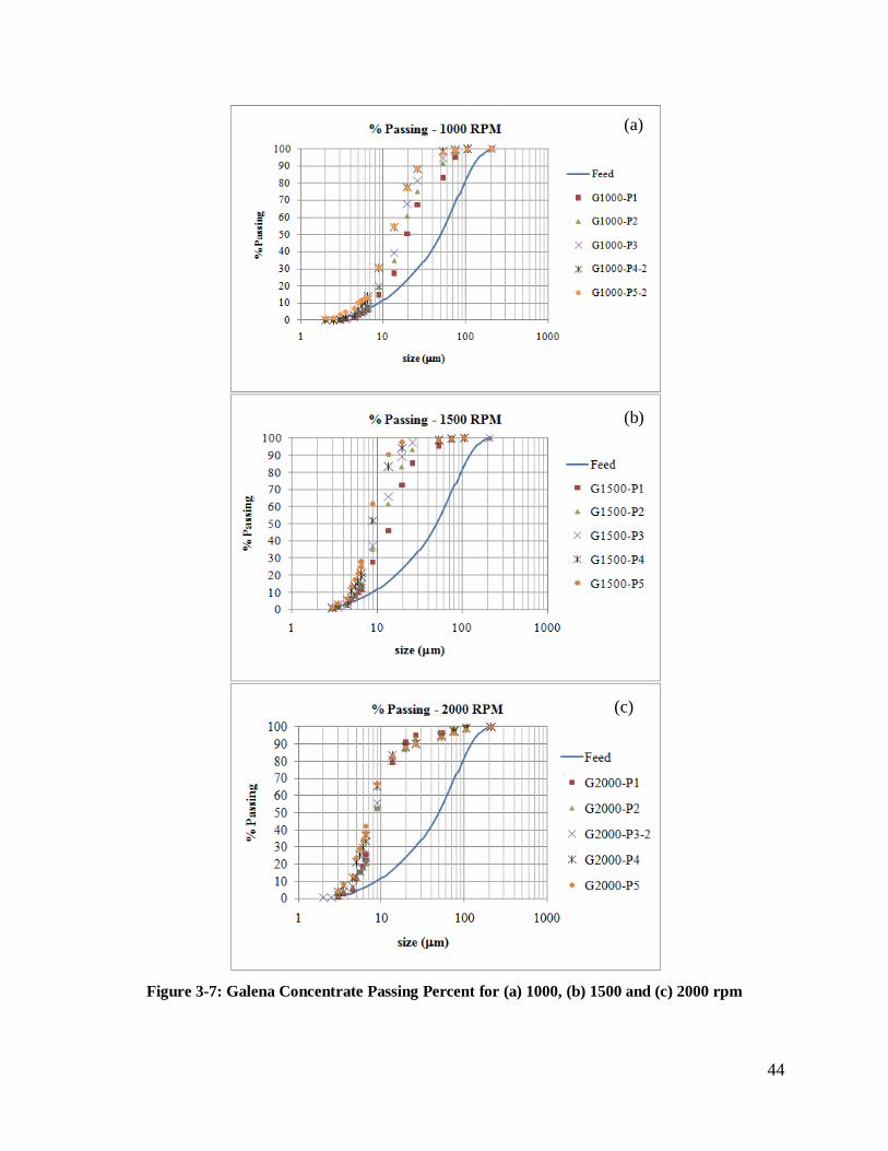
44
Figure 3-7: Galena Concentrate Passing Percent for (a) 1000, (b) 1500 and (c) 2000 rpm
(a)
(b)
(c)

45
Figure 3-8: Mixed Quartz and Galena Sample Passing Percent for
(a) 1000 and (b) 2000 rpm
(a)
(b)

46
Figure 3-9: Lead-Zinc Ore Sample Passing Percent for (a) 1000, (b) 1500 and (c) 2000 rpm
(a)
(b)
(c)
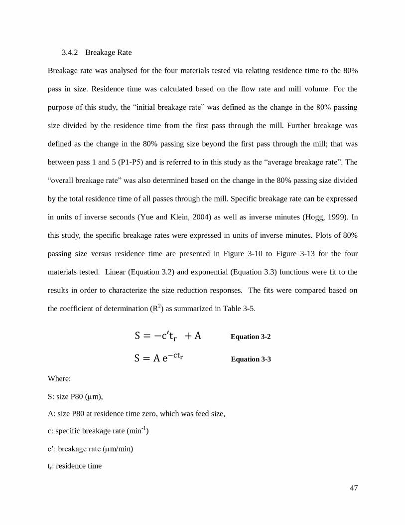
47
3.4.2 Breakage Rate
Breakage rate was analysed for the four materials tested via relating residence time to the 80%
pass in size. Residence time was calculated based on the flow rate and mill volume. For the
purpose of this study, the ―initial breakage rate‖ was defined as the change in the 80% passing
size divided by the residence time from the first pass through the mill. Further breakage was
defined as the change in the 80% passing size beyond the first pass through the mill; that was
between pass 1 and 5 (P1-P5) and is referred to in this study as the ―average breakage rate‖. The
―overall breakage rate‖ was also determined based on the change in the 80% passing size divided
by the total residence time of all passes through the mill. Specific breakage rate can be expressed
in units of inverse seconds (Yue and Klein, 2004) as well as inverse minutes (Hogg, 1999). In
this study, the specific breakage rates were expressed in units of inverse minutes. Plots of 80%
passing size versus residence time are presented in Figure 3-10 to Figure 3-13 for the four
materials tested. Linear (Equation 3.2) and exponential (Equation 3.3) functions were fit to the
results in order to characterize the size reduction responses. The fits were compared based on
the coefficient of determination (R2) as summarized in Table 3-5.
Equation 3-2
Equation 3-3
Where:
S: size P80 (m),
A: size P80 at residence time zero, which was feed size,
c: specific breakage rate (min-1
)
c’: breakage rate (m/min)
tr: residence time

48
The overall coefficient of determination (average) was higher for the linear model than the
exponential model for quartz and mixed quartz and galena sample. On the other hand, the R2
value for exponential model was higher than the linear model for the galena concentrate sample
and slightly higher for lead-zinc ore sample. This implied that the type of mineral had an effect
on the breakage rate trend, linear versus exponential.
Figure 3-10: Quartz (a) Linear and (b) Linearized Exponential Fitting Data
0
20
40
60
80
100
0 1 2 3 4 5 6
P8
0 (
m)
Residence Time (min)
Linear Quartz
Feed
Q1000
Q1500
Q2000
0.0
1.0
2.0
3.0
4.0
5.0
0 1 2 3 4 5 6
Ln
P8
0 (
m)
Residence Time (min)
Linearized Quartz
Feed
Q1000
Q1500
Q2000
(a)
(b)

49
Figure 3-11: Galena Concentrate (a) Linear and (b) Linearized Exponential Fitting Data
0
20
40
60
80
100
0 1 2 3 4 5 6
P8
0 (
m)
Reidence Time (min)
Linear Galena Concentrate
Feed
G1000
G1500
G2000
0.0
1.0
2.0
3.0
4.0
5.0
0 1 2 3 4 5 6
Ln
P8
0 (
m)
Residence Time (min)
Linearized Galena Concentrate
Feed
G1000
G1500
G2000
(a)
(b)

50
Figure 3-12: Mixed Quartz and Galena Sample (a) Linear and
(b) Linearized Exponential Fitting Data
0
20
40
60
80
100
120
140
0 1 2 3 4 5 6
P8
0 (
m)
Residence Time (min)
Linear Mixed Sample
Feed
M1000
M2000
0.0
1.0
2.0
3.0
4.0
5.0
6.0
0 1 2 3 4 5 6
Ln
P8
0
Residence Time (min)
Linearized Mixed Sample
Feed
M1000
M2000
(a)
(b)

51
Figure 3-13: Lead-Zinc Ore Sample (a) Linear and
(b) Linearized Exponential Fitting Data
0
20
40
60
80
100
0 2 4 6
P8
0 (
m)
Residnece Time (min)
Linear Lead-Zinc Ore
Feed
O1000
O1500
O2000
0.0
1.0
2.0
3.0
4.0
5.0
0 1 2 3 4 5 6
Ln
P8
0 (
m)
Residence Time (min)
Linearized Lead-Zinc Ore
Feed
O1000
O1500
O2000
(a)
(b)
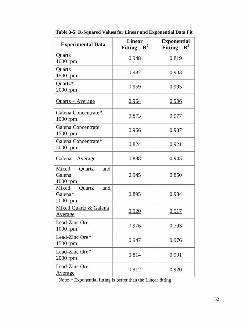
52
Table 3-5: R-Squared Values for Linear and Exponential Data Fit
Experimental Data Linear
Fitting – R2
Exponential
Fitting – R2
Quartz
1000 rpm 0.948 0.819
Quartz
1500 rpm 0.987 0.903
Quartz*
2000 rpm 0.959 0.995
Quartz – Average 0.964 0.906
Galena Concentrate*
1000 rpm 0.873 0.977
Galena Concentrate
1500 rpm 0.966 0.937
Galena Concentrate*
2000 rpm 0.824 0.921
Galena – Average 0.888 0.945
Mixed Quartz and
Galena
1000 rpm
0.945 0.850
Mixed Quartz and
Galena*
2000 rpm
0.895 0.984
Mixed Quartz & Galena
Average 0.920 0.917
Lead-Zinc Ore
1000 rpm 0.976 0.793
Lead-Zinc Ore*
1500 rpm 0.947 0.976
Lead-Zinc Ore*
2000 rpm 0.814 0.991
Lead-Zinc Ore
Average 0.912 0.920
Note: * Exponential fitting is better than the Linear fitting

53
Data correlation charts for overall breakage rate are presented in Figure 3.14. Initial breakage fit
equally well for both linear and exponential. The average breakage fitted reasonably well with
both the linear and exponential equations, (Appendix B3). Analysis of the overall breakage
showed a better exponential rate fit compared to the linear fit. The galena concentrate and the
lead-zinc ore had the poorest fit, particularly at higher agitator speeds. The reason for the poor
data fit was that the product reached its grinding limit faster than the other material tested.
Therefore, the calculated data points don’t have a matching experimental, measured value.
Figure 3-14: Correlation Between Measured and Calculated P80 for
Overall Breakage Rate Data; (a) Quartz, (b) Galena Concentrate,
(c) Mixed Quartz and Galena Concentrate Sample and (d) Lead-Zinc Ore Sample
Note: The initial and average breakage rate correlation plots are presented on Appendix B3
(a) (b)
(c) (d)

54
3.4.2.1 Initial Breakage Rate
Since initial breakage showed a different trend than the average breakage, breakage rate values
were calculated for both, and presented in Table 3-6. The trend showed that quartz, galena
concentrate, mixed quartz and galena sample and lead-zinc ore sample initial breakage rates
increased linearly with the increase of input energy (agitator speed). Softer mineral breakage rate
values were higher than the harder ones by approximately one order of magnitude. For example,
the galena concentrate breakage rate at 1000 rpm was 0.78min-1
compared to the quartz which
was only 0.07min-1
. It was also observed that the mixed quartz and galena sample breakage rate
was closer to the pure quartz than the pure galena concentrate samples. Also, at the lowest stirrer
speed (1000 rpm) the breakage rate for both the quartz and the mixed quartz and galena samples
was low which reflected that the energy input was not sufficient to promote breakage. The initial
breakage rate for softer minerals was faster than for the harder minerals at the three agitator
speeds tested.
Table 3-6: Initial and Average Breakage at Different Agitator Speed
RPM
Specific Breakage Rate
(min-1)
Quartz Galena
Concentrate Mixed Sample Lead-Zinc Ore
Initial Average
Breakage Initial
Average
Breakage Initial
Average
Breakage Initial
Average
Breakage
1000 0.07 0.05 0.78 0.25 0.02 0.05 0.63 0.22
1500 0.18 0.22 1.34 0.16 --- --- 0.90 0.34
2000 0.35 0.32 1.82 0.02 0.36 0.37 1.34 0.32

55
3.4.2.2 Average Breakage Rate
The effect of the increasing grinding residence time on breakage rate was represented by the
average breakage rate. Increasing the grinding residence time had a minimal effect on breakage
rate for quartz and mixed quartz and galena sample, but decreased for the galena concentrate
sample and the lead-zinc ore sample. Residence time and agitator speed were directly
proportional to the average breakage rate for the quartz and mixed sample, but inversely
proportional for the galena concentrate sample. For the lead-zinc ore sample, average breakage
rate increased with the increase of the agitator speed from 1000 to 1500 rpm and then decreased
slightly at the 2000 rpm agitator speed. The average breakage rate was affected by the grinding
limits for the materials and test conditions. The softer samples (galena concentrate and to some
extent the lead-zinc ore samples) had high initial breakage rates and therefore approached their
grinding limit faster than harder minerals. Parry (2006) stated that soft minerals broke faster at
lower agitator speeds than hard minerals, but the breakage rates for hard and soft minerals
converge at very high agitator speed. Similar conclusions could be deduced from the data
obtained from this set of experiments.
For the quartz sample, the breakage rate curve changed from linear to exponential when
increasing the stirrer speed from 1500 rpm to 2000 rpm. For the galena, the breakage rate data
fit the non-linear breakage equation at a lower agitator speed of 1000 rpm. Therefore, both the
hard and soft minerals responded in a similar manner, but at different stirrer speeds. The
breakage rate values could lead to a preliminary conclusion that if the target was to grind the
softer mineral in a mix of hard and soft minerals, then the choices would either be to operate the
mill at a low agitator speed, such that, the soft mineral would break and the hard mineral would
not, or operate the mill at a higher agitator speed for a shorter residence time. Similar conclusion

56
is observed by Parry (2006), who tested quartz and magnetite as hard minerals and calcite as soft
mineral, and concluded that soft minerals do break faster as lower agitator speeds than hard
minerals.
3.4.3 Energy Consumption
The grinding mechanism in the stirred mill is through agitating the slurry material in the mill
using agitator discs. Accordingly, energy is transmitted from the agitator to the grinding media
and the slurry. Then abrasion, compression and impact loadings are applied to the particles. In
other words, kinetic energy was transmitted from the shaft to the particles in the mill (media and
minerals). Thus increasing or decreasing the agitator speed (kinetic energy input) directly affects
the amount and type of loading applied on the particles which would consequently lead to
particle breakage and size reduction. Specific energy is calculated by subtracting the power of
the mill with no load from the power of the mill with load, multiplied by the residence time per
mill volume. The powers used in the calculations are read from the agitator panel, which is the
input power direct to the agitator with and without load. This is a typical industrial practice to
scale up stirred mills based on energy versus size reduction. The log-log plot of the specific
energy input versus size reduction (P80) produces linearized data which fit a power equation that
is called a signature plot. Signature plots are used for scaling up stirred mill machines from a lab
scale to an industrial scale. Most of the data have a curve trend which could fit either to a power
or exponential fit equation as per equation 3-4 or equation 3-5, respectively. For the power
function, a variable base is raised to a fixed exponent, whereas for the exponential function, a
fixed base is raised to a variable exponent.

57
Equation 3-4
Equation 3-5
Where:
Psp: specific power (KWhr/ton)
Po: specific power at size zero; hypothetical
S: size P80 (m),
d: specific power per size reduction
Experimental data did not fit the power equation as well as expected for all test runs. Therefore,
data were also fit to the exponential equation for comparison. As presented in Table 3-7, when
comparing the coefficient of determination (R2 values) for both types of equation fittings, it
showed that the exponential equations fit better than the power equation for the four materials
tested at low and medium agitator speeds, 1000 and 1500 rpm, respectively. At a higher agitator
speed of 2000 rpm, the power equation fit the data slightly better.
Table 3-7: R2 Values for Specific Energy vs. Size Reduction Using Power
and Exponential Equations
Power and exponential equation fits were plotted for quartz, galena concentrate, mixed quartz
and galena concentrate sample, and lead-zinc ore sample, as shown in Figure 3-15, Figure 3-16,
Power Exponential Power Exponential Power Exponential Power Exponential
1000 RPM 0.821 0.835 0.978 0.988 0.879 0.883 0.796 0.851
1500 RPM 0.880 0.937 0.940 0.965 --- --- 0.972 1.000
2000 RPM 0.996 0.986 0.920 0.918 0.978 0.994 0.990 0.954
Combined 0.829 0.915 0.897 0.805 0.900 0.971 0.939 0.963
Agitator Speed
(rpm)
Quartz Galena Mix Ore

58
Figure 3-17 and Figure 3-18, respectively. The cumulative data trend combined for the three
agitator speeds per each material type were also plotted.
Figure 3-15: Quartz Signature Plot – (a) Exponential and (b) Power Fit
The quartz signature plot results supported the interpretation of PSD plot for the 1000 rpm test. It
indicated that the agitator speed had a limiting grinding ability, as shown in Figure 3-6(a) no
matter how much more input power was given to the material. The exponential equations for all
cumulative data from the three agitator speeds fit the data better than the power equations. This
was identified by a higher R2 value (0.915) for the exponential equation, compared to the power
equation R2 value, which was 0.829, as illustrated in Figure 3-15. It was also noticed that the
specific energy required to target a certain size reduction (P80) was overlapping among the three
agitator speeds. The 1500 rpm initial breakage (1st pass) overlapped with the 1000 rpm at the 4
th
pass. The 2nd
pass of the 1500 rpm was overlapping with the 2000 rpm at the 1st pass. The
overlap between data at the three agitator speeds indicated that the effect of the agitator speed on
the signature plot was insignificant, compared to the breakage rate effect.
Data Overlap
(a) (b)

59
Figure 3-16: Galena Concentrate Signature Plot – (a) Exponential and (b) Power Fit
The galena concentrate signature plot also helped to explain the PSD results at 2000 rpm, where
the grinding limit was reached immediately after the first pass (54 seconds residence time).
Increasing power input, in the form of increasing residence time, did not significantly affect
particle size reduction at the high agitator speed (2000 rpm). For the low agitator speed (1000
rpm), the last two passes (4th
and 5th
) showed similar size values, with minor increase in energy
input. This implied that grinding limit had been reached using a low agitator speed. However, if
additional runs were done, it would have confirmed the grinding limit of the galena; it is
expected that the energy consumption would have increased without a reduction in product
particle size.
The galena concentrate (soft) responded in an opposite manner to that of quartz (hard). The
combined R2
value for galena concentrate fitted the power equation better than the exponential
equation while for quartz the combined R2
values fitted the exponential equation better than the
power equation. It was also noticed that the combined R2 value for both the power and
exponential equations for galena concentrate were consistently lower than the individual R2 for
y = 11238x-2.459
R² = 0.8966
y = 3657.7x-2.124
R² = 0.9547
1
10
100
10 100
Sp
ecif
ic E
nerg
y (
kW
hr/t
on
)
Size P80 (m)
Galena Concentrate - Power
G1000 G1500 G2000 Power (Cumulative) Power (Cumulative 1000 & 1500)
(a) (b)

60
each agitator speed. Similarly, the quartz followed the same trend as the galena concentrate
except for the low agitator speed (1000 rpm), which had a lower R2 value compared to the
combined values as per Table 3-7. Such results would imply that the individual set of data for
each agitator speed created a different trend. Such an observation was graphically confirmed in
Figure 3-16. The high speed (2000 rpm) data were excluded from the combined analysis because
the grinding limit was reached almost immediately after the first pass. The results showed that
changing the stirrer speed shifted the signature plot. For example, at about 5kwhr/t specific
energy, the lower agitator speed (1000 rpm) created finer product than the same specific energy
for the intermediate agitator speed (1500 rpm). If the grinding process was targeting a certain
size fraction, such as 13m, the high agitator speed (2000 rpm) would consume more specific
energy (19 kwhr/t) compared to the intermediate agitator speed, which consumed 15 kwhr/t. The
agitator speed had a significant effect on the signature plot and breakage rates of the galena
concentrate material.
Figure 3-17: Mixed Quartz and Galena Sample Signature Plot
(a) Exponential and (b) Power Fit
(a) (b)

61
Due to a shortage in material availability, the mixed quartz and galena sample test runs were
executed on only the extreme agitator speeds, 1000 and 2000 rpm. The exponential equation fit
the data slightly better than the power equation in terms of their R2
values, 0.971 and 0.900,
respectively. The cumulative trend, as in Figure 3-17, showed that there was a potential for
continuity between the two agitator speeds, despite the gap between them. This gap could have
been covered by increasing the residence time of the particles in the mill, especially for the 1000
rpm test run. The mixed quartz and galena concentrate sample trend was similar to the trend for
the quartz material.
Figure 3-18: Lead-Zinc Ore Sample Signature Plot – (a) Exponential and (b) Power Fit
For the lead-zinc ore sample, specific energy versus size reduction followed a continuous
pattern, except for the fifth pass for the 1000 and 1500 rpm test runs. The exponential equation
fit the data slightly better than the power equation, as shown by the R2 values, which were
0.9634 and 0.9393, respectively. The combined R2 values for power and exponential equations
were higher than the individual R2
values for the low agitator speed (1000 rpm), which indicated
a trend for low agitator speeds that deviated from the other two agitator speeds. The plots
Data Overlap
Target size ~ 17m Data Overlap
(a) (b)

62
showed that there was a minor overlap between the data at the three agitator speeds. The
overlaps were identified at the initial breakage (1st pass) of the intermediate agitator speed (1500
rpm), and the 4th
pass of the lower agitator speed (1000 rpm), as shown in Figure 3-18(a).
Similar overlap was noticed at the initial breakage (1st pass) of the high agitator speed (2000
rpm), and the 2nd
pass of the intermediate agitator speed (1500 rpm). Overlap was also noticed at
the 2nd
pass and the 4th pass of the high agitator speed (2000 rpm), and intermediate agitator
speed (1500 rpm), as shown in Figure 3-18(b), respectively. The lower agitator speed reached a
similar size at a lower specific energy input, as with the 17m target size shown in Figure 3-
19(a).
The specific energy analysis showed that there was overlapping in the energy required versus
targeted size reduction between the different agitator speeds; however, the overlap was not
consistent. The analysis also demonstrated that the data fit differently to the power and
exponential equations, based on the type of material and agitator speed selected for grinding. The
effect of the agitator speed on the signature plot was a function of the material type. It was
believed that the grinding limit was not reached for all the test runs carried out on the 4 materials
tested and at the agitator speeds chosen. If more passes were performed, a complete analysis
could have been achieved. However, reaching the grinding limit was not the scope of this
research. The amount of samples collected were enough for the scope and focus of this study
which is the morphology analysis.
3.4.4 Effective Energy
Energy usage that is transmitted from the agitator discs into stirring of the slurry is the effective
energy which creates the particles dynamics in the mill. The particles dynamics in the mill
generates the forces that are translated into stresses. When the stresses exceed the critical stress

63
intensity values, breakage initiates or propagates. The net energy is the total energy consumed
by the mill with-load minus the energy consumed with no-load. The ―no load‖ energy is the
energy required to rotate the agitator of the mill with no media or slurry. The net energy is the
energy needed to agitate the slurry and break particles. The ratio of the net energy to the total
energy input to the system is an indication of the effective energy applied to the slurry. The unit
of the effective energy was reported in this study as Joules. Similar comparison was attempted
using a DEM computer model of the IsaMill, which is described in details in chapter 5. The net
energy from the experimental work was equivalent to the total kinetic plus rotational kinetic
energies of the particles captured at each time step of the simulation runs. In the computer model,
such energy was referred to as the output energy. The total energy from the experiments was
equivalent to the input energy to the mill from the computer model, which was the cumulative
agitator torque for all time steps. Section 5.4.1.2 further describes the energy distribution in the
mill using DEM. The net energies versus total energies are plotted in Figure 3-19. The slopes
signified the effective energy ratio.

64
Figure 3-19: Grinding Effective Energy for (a) Quartz, (b) Galena Concentrate,
(c) Mixed Sample and (d) Lead-Zinc Ore Sample
According to the plots in Figure 3-19, the agitator speed had a more considerable effect on the
energy ratio than type of material being ground. It was observed that the higher the agitator
speed, the higher the effective energy ratio. The average effective energy ratio values for the four
materials tested were 0.3, 0.5 and 0.6 for agitator speeds 1000, 1500 and 2000 rpm, respectively.
The higher the agitator speed, the better use of the energy input to the mill during the grinding
process. The effective energy analysis indicated that it is a function of agitator speed rather than
material being ground.
(a) (b)
(c) (d)

65
3.4.5 Specific Breakage Energy
For the purpose of this study, specific breakage energy is presented as the amount of energy
required to reduce a particle size by one micron. The net energy was plotted versus particle size
(P80) for each material tested at different agitator speeds (Appendix B4). The slope is the ratio of
the net energy input per particle breakage. The specific breakage energy values are listed in
Table 3-8. The initial breakage energy for quartz, a hard mineral, increased linearly with the
increase of the agitator speed. On the other hand, the initial breakage energy for galena, a soft
mineral, increased exponentially with the increase of the agitator speed. Comparing the same
agitator speeds showed that galena consumed about 5.5 times less energy per particle breakage
than the quartz at low agitator speed (1000 rpm). At intermediate agitator speed (1500 rpm),
galena consumed about 3 times less energy per particle than quartz and at the high agitator speed
(2000 rpm), galena consumed 2 times less energy per particle breakage than quartz. This implied
that for initial breakage, the galena consumed less energy to break at all agitator speeds.
The average specific breakage energy is the specific energy after 5 passes, which corresponds to
a longer residence time of the material in the mill. The average specific breakage energy showed
that galena consumed about 2.3 times less energy per particle breakage than quartz. Whereas at
intermediate agitator speed (1500 rpm), galena consumed 4.4 times more energy per particle
breakage than quartz, and at high agitator speed (2000 rpm) galena consumed 52 times more
energy per particle breakage than quartz. The reason for the increase of energy consumption per
particle by galena was that it reached its grinding limit early in the grinding process, mostly
during the initial breakage. If the particles were exposed to more grinding by increasing their
residence time in the mill, after reaching their grinding limit, it would lead to useless energy
consumption.

66
The mixed quartz and galena sample responded in similar manner to the quartz at a high agitator
speed (2000 rpm) for both initial and average breakage. At a low agitator speed (1000 rpm), the
initial breakage seemed to consume higher energy than both galena and quartz, which implied
that there was hardly any breakage occurring. The specific breakage energy of the lead-zinc ore
sample was increasing with the increase of the agitator speed, but showed lower values than the
galena concentrate sample. This implied that the effect of the mix of minerals in the ore had a
significant effect on the amount of energy required per unit micron breakage.
Table 3-8: Specific Breakage Energy (kJ/m)
Agitator
Speed
(rpm)
Quartz
(kJ/m)
Galena
Concentrate
(kJ/m)
Mixed sample
(kJ/m)
Lead-Zinc Ore
Sample
(kJ/m)
Initial Average Initial Average Initial Average Initial Average
1000 1.83 2.79 0.33 1.18 6.82 1.74 0.24 1.08
1500 2.94 3.47 0.96 15.3 --- --- 0.78 3.93
2000 3.40 6.05 1.85 314.0 3.11 5.06 1.42 11.4
3.5 Conclusion
The effect of the material properties, mill input energy in the form of agitator speeds, and
residence time was investigated through a series of experiments.
Results showed that the material type had a major effect on particle size distribution and size
reduction at the three agitator speeds evaluated. Quartz did not break efficiently at the 1000 rpm
agitator speed, which indicated that there was a minimum energy input required to initiate the
breakage. On the other hand, 1000 rpm was enough for the galena concentrate to break. The
extreme agitator speed, 2000 rpm, broke the galena concentrate particles down to its grinding
limit after the first pass through the mill. For the mixed sample, the quartz breakage mechanism

67
effect was dominant over the galena due to the higher content of quartz in the mix compared to
galena, 6:1 ratio.
Initial breakage rates of the 4 materials tested increased linearly with the increase of the agitator
speed. However, breakage rates were almost one order of magnitude higher for the soft minerals
than the hard minerals. Average breakage values were directly affected by how close the particle
sizes were from their grinding limit. Breakage rate decreased once it reached the grinding limit
of the material.
The breakage rate was linear for most of the grinds except for quartz at 2000 rpm, galena
concentrate at 1000 rpm, mixed quartz and galena sample at 2000 rpm and lead-zinc ore sample
at 1500 and 2000 rpm. The aforementioned test runs and material exhibited a nonlinear breakage
rate. This observation indicated that breakage rate trend is non-linear when it approaches the
grinding limit of the material.
Energy consumption was evaluated using typical signature plots, which are specific energy
versus size reduction (P80). It was observed that there was some overlapping in the energy
required versus targeted size between the different agitator speeds; however, the overlapping was
not consistent. The analysis also revealed that the data fit differently to the power and
exponential equations, based on the type of material and agitator speed selected for grinding. It
was also observed that the effective energy ratio of the mill was not affected by the type of
material as much as it was affected by the agitator speed. The highest effective energy ratio was
observed at the highest agitator speed. On the other hand, the amount of energy required to break
one micron was directly affected by the type of material being ground. Soft minerals required

68
less energy per micron at all agitator speeds. Thus, the softer minerals would break faster at
lower agitator speed than harder minerals and vice versa.

69
4. Morphology and Liberation
4.1 Introduction
4.1.1 Morphology Definition
Morphology is the study of particle shape and texture. Particle shape is a factor of equivalent
diameter, sphericity, convexity, aspect ratio and roughness. Morphology analysis software
measures basic parameters such as particle length, width, perimeter from pre-captured images,
either through optical microscopes or scanning electron microscopes (SEM). Software such as
Clemex uses standard mathematical equations to deduce more complex morphological
parameters, such as sphericity, elongation, aspect ratio, roughness and others.
4.1.2 Morphology Evaluation
Studies performed on particle morphology analysis for different grinding processes have been
addressed by Gabriel (1985), Pons et. al. (1999), Hiçyilmaz et al. (2004), Yekler et. al. (2004),
Ulusoy and Yekeler (2005), Celik & Oner (2006); Kursun and Ulusoy (2006), Guimaraes et al.
(2007), Tavares and Das Neves (2008), Hasanpour and Choupani (2009). These analyses were
either qualitative or quantitative. Qualitative analysis is a visual comparison of captured high
resolution images via SEM, such as the stirred bead mill of gibbsite research performed by Alex,
et. al. (2008), and a study on aggregate production during rock crushing by Guimaraes, et.
al.(2007). For quantitative analysis, morphological parameters are measured such as elongation,
sphericity, and roughness as those performed by Lecoq et. al (1999) and Donskoi et al. (2007).

70
Typical equations used for quantitative morphology analysis are as follows, Clemex
Technologies Inc. (2009):
Elongation = 1 / AR
Note: Sphericity is the circularity squared, which is the equivalent circumference squared
(perimeter squared) of a measured surface area, divided by the actual perimeter.
Convexity is a parameter used to evaluate particle roughness. Convexity is the ratio between the
hull perimeter and the actual measured perimeter. The hull perimeter (HP) is the measure of the
contour of the extrude edges of the particle as shown in Figure 4-1
Figure 4-1 Particle Perimeter and Hull Perimeter
Where:
L: length
W: width
A: area
S: sphericity
P: perimeter
HP: hull perimeter
AR: aspect ratio
Equation 4-1
Equation 4-2
Equation 4-4
Equation 4-3
Equation 4-5
Equation 4-6
HP
P

71
The major parameters of interest for this research were roughness, sphericity and elongation
values. The values of such parameters range from zero to one. For roughness, a value of one
reflects a perfectly smooth particle, since the hull perimeter would coincide with the actual
perimeter. Similarly, if the sphericity value is one, then the calculated perimeter from the surface
area would be equivalent to the actual measured perimeter. For elongation, a value of one
reflects an equiaxed particle since the particle’s width would be equal to its length. Values close
to zero, for all three parameters, means that the particles are rougher, less circular and more
elongated.
The roughness level assessed using pre-programmed morphology software (Clemex) was not
precise enough for 3D images captured via SEM when compared to 2D images. The software
evaluated the outer contour of the particles, ignoring the surface texture. Accordingly, the values
were biased towards smooth particles rather than rough particles. Therefore, the manual point
count methodology was developed. Since roughness was the major parameter to be assessed in
this research, both methodologies were evaluated and compared.
4.1.3 Sample Description for Morphology
The samples used for morphology analysis were classified according to their size fraction, as
coarse, medium and fine. The coarse fraction was a product of screening, and the geometric
mean particle size was 63m for the four materials analysed: quartz, galena concentrate, mixed
quartz and galena concentrate, and lead-zinc ore. The medium and fine fractions were produced
via Cyclosizer, which resulted in different size fractions based on the mineral density. For the
sake of comparison, the size fraction for each material was chosen based on the particle size,
rather than the Cyclosizer cyclone number. Therefore, the geometric mean size for quartz, galena
concentrate, mixed quartz and galena sample, and lead-zinc ore samples were 34, 37, 36 and

72
33m for the medium size fraction and 15, 17, 18 and 16m for the fine size fraction,
respectively. Details on sample preparation of size fractions are presented in chapter 3, section
3.3.4.
4.2 Clemex Method
The roughness of the particles suggests the mode of particle breakage. It could be due to impact,
abrasion or compression loading. If the particles are exposed to abrasion, they would exhibit
smoother and more rounded surfaces. On the other hand, if they are exposed to compression or
impact loading, they would reveal rougher and less round surfaces. The theory is that if the
particles are exposed to enough impact or compression forces, they would break along their
weakest planes, that is their grain boundaries, and show intergranular breakage. Abrasion, on the
other hand, would cause a polishing effect, creating smooth particles with breakage across the
grains – transgranular breakage.
The procedure followed to evaluate the particles’ morphology features started by capturing high
resolution 3D images via SEM - back scatter beam. Images were then imported into the Clemex
software, followed by running a routine that recognizes the particles, and calculates their main
morphology parameters (sphericity, elongation and roughness). Measured and calculated data
were then exported to an excel format for further analysis. The detailed Clemex routine is
provided in Appendix C4.
By assessing the values of roughness, it was noticed that the Clemex results were biased towards
higher values, indicating smoother particles, as compared to visual observation. For example, the
particles that were given a roughness value of 0.9 (closer to a smooth value) were visually
identified to have exhibited extremely rough surfaces. An example of this observation is

73
presented in Figure 4-2. The particles in this figure are from the +53m fraction of the quartz
sample prior to stirred milling. The Clemex identified their roughness values as 0.9 and 1.0,
which would be categorized as smooth particles, whereas visual examination would identify their
roughness values as 5 and 4, which would categorize them as very rough particles. There could
be two possible reasons for this observation. Either the Clemex recognised the particles in 2-D
(outer contour of the particles), and ignored their actual surface texture, or the software over-
iterated the convex perimeter (Feret Iteration), which ended up very close to the particles’ actual
perimeter.
Figure 4-2: (a) Particle ID 39 Roughness value was 0.9;
(b) Particle ID 14 Roughness value was 1.0
Feret is a measure of the distance between two parallel tangent lines at a defined angle. The
convex perimeter is the measure of a rubber band around all the ferets. The greater the number of
ferets measured at multiple angles, the closer the hull perimeter value would be to the actual
perimeter. This measurement would return a roughness value closer to 1 (smooth particle).
Therefore, a manual point counting methodology was introduced and tested in this study.
a b

74
4.3 Manual Point Counting Method
As an alternative to the Clemex software, manual point counting was tested. The roughness
values were set to 5 levels: R1, R2, R3, R4, and R5. The roughest particle was given a value of 5,
where as the smoothest particle was given a value of 2. The degree of roughness increased from
2 to 5. Roughness level 1 was given to surfaces that were round, with no sharp edges, but had a
hammered surface. It was speculated that the same particle was exposed to some type of
compressive loading. Detailed definitions and illustrations of roughness levels for quartz and
galena are presented in Table 4-1. An excel macro subroutine was built using visual basic to
assist in the counting process, and its details are given in Appendix C1 and C2. The subroutine
accumulated the counts for the roughness values between 1 and 5. After the counter was
familiarized with the definitions of the roughness levels for the particles, a grid was placed on
the SEM printed images in order to assist in tracing and counting the particles’ degree of
roughness.

75
Table 4-1: Morphology Roughness Level Definitions and Illustration
Roughness
Level Definition
Illustration
Quartz Galena
R1
Hammered
Round but hammered
surface.
R2
Smoothest
Round and less rough
surfaces.
R3
Semi-Rough
Partially round, partially
angled and partially rough
surfaces.
R4
Rougher
- For quartz: partially
round and rougher
surfaces.
- For Galena: square
edges
R5
Roughest
Rough and sharp angled
surfaces.

76
4.3.1 Point Counting Sensitivity Analysis
To assess sensitivity, three counters were trained on evaluating the particles’ degree of
roughness. Each performed the counting procedure on the same sample, and results were then
compared. The first counting attempt showed that the degree of roughness definition for R2, R3
and R4 was not adequately identified by the counters. The roughness level definitions were fine
tuned and re-defined, as per Table 4-1, and the counting procedure was repeated. Results were
compared among the three counters, and results showed that a very close match between the
three individuals was achieved, with a maximum difference of 6%. The process was repeated on
different size fractions in order to verify the results (53m and 14m particles). Detailed
counting results of the sensitivity analysis are presented in Appendix C3.
4.4 Liberation Methodology
The fourth material tested was the lead-zinc ore sample, which was a complex ore that has
similar mineral composition to that of the synthesised mixed quartz and galena sample.
However, it contained un-liberated composite particles. The objective of this part of the study
was to understand the liberation behaviour of the minerals under different stress intensity input
(i.e. different agitator speeds). The Mineral Liberation Analyser (MLA) is a conventional tool
used for liberation analysis. A representative sample is placed in an epoxy resin, which is then
ground and polished, in order to expose a monolayer of the particles in a 2D format. This process
creates a cross section surface through the particles. The samples are then placed in an SEM,
which is equipped with Mineral Liberation Analysis software (MLA) that scans and analyses the
identified mineral particles and their associations.
The MLA process was costly and time consuming. Furthermore, this research was focused on
analysing the particles as fractured, without sectioning them, since morphology was the core of

77
this study. Accordingly, liberation analysis was performed on a stud sample where the particles
were first spread on a glass sheet in order to create a monolayer. The particles were then picked-
up on a double graphite sticky sheet on a stud. The sampling type was called ―as mount‖
samples. The same analysis procedure using the SEM-MLA was performed. Analysis was
performed following the first stage of grinding for the lead-zinc ore samples from the three
agitator speed grinds (O1000-P1, O1500-P1 and O2000-P1). The size fraction tested was -75m
+53m.
Since the ―as mount‖ procedure was not a conventional method, it was important to compare the
conventional, resin mount polished sample with the ―as mount‖ procedures. Samples used for
comparison were the -75m +53m size fraction, which has a geometric mean size of 63m
from the 1500 rpm stirrer speed test run. Sample from 3 passes through the mill were enough to
compare the trend of the ―as mount‖ to the conventional method.
4.5 Morphology and Liberation Results
The effect of mineral properties and mill operation on breakage mechanisms could be identified
by analysing the product morphology. Due to the biased results of the pre-programmed image
analysis software, explained in section 4.2, manual point counting and automated (pre-
programmed) morphology analysis were both performed, for the sake of comparison and
confirmation of the outcome results. Manual point counting was executed on 3 size fractions for
each material (coarse, medium and fine), and the automated morphology analysis was executed
on the coarse size fraction (geometric mean size is 63m).

78
4.5.1 Manual Point Counting Results
Manual point counting was based on five levels of roughness as described in section 4.3.
Roughness levels start with R1 as a round and hammered surface, R2 as the smoothest, round
particles, R3 as the bridge between the smooth and rough particles which was labelled as semi-
rough particles, R4 as a rough particle with few round surfaces, and R5 as the roughest particle
with all sharp and angled surfaces. Detailed roughness levels and their descriptions are presented
in Table 4-1. Relationships between the roughness level and mode of breakage were predicted
such that the rougher the particles, the higher the potential for intergranular breakage was to
occur. One could reasonably suggest that for smoother particles, the breakage mode was abrasion
(transgranular), whereas for rougher particles, the breakage mode could be fracture via impact or
compression loading (intergranular – along grain boundaries). Detailed breakage modes versus
roughness levels are outlined in Table 4-2.
Table 4-2: Breakage Mode versus Roughness Level
Roughness
Level Breakage Mode
R1
Hammered
- Started Abrasion
(Transgranular)
- Then Exposed to Impact
(Indents on Surface)
R2
Smoothest
Abrasion
(Transgranular)
R3
Semi-Rough
Exposed to both Abrasion and Fracture
(Transgranular and Intergranular)
R4
Rougher
Fracture
(Intergranular)
R5
Roughest
Fracture
(Intergranular)
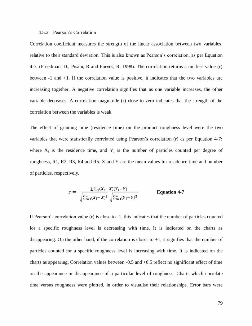
79
4.5.2 Pearson’s Correlation
Correlation coefficient measures the strength of the linear association between two variables,
relative to their standard deviation. This is also known as Pearson’s correlation, as per Equation
4-7, (Freedman, D., Pisani, R and Purves, R, 1998). The correlation returns a unitless value (r)
between -1 and +1. If the correlation value is positive, it indicates that the two variables are
increasing together. A negative correlation signifies that as one variable increases, the other
variable decreases. A correlation magnitude (r) close to zero indicates that the strength of the
correlation between the variables is weak.
The effect of grinding time (residence time) on the product roughness level were the two
variables that were statistically correlated using Pearson’s correlation (r) as per Equation 4-7;
where Xi is the residence time, and Yi is the number of particles counted per degree of
roughness, R1, R2, R3, R4 and R5. X and Y are the mean values for residence time and number
of particles, respectively.
–
Equation 4-7
If Pearson’s correlation value (r) is close to -1, this indicates that the number of particles counted
for a specific roughness level is decreasing with time. It is indicated on the charts as
disappearing. On the other hand, if the correlation is closer to +1, it signifies that the number of
particles counted for a specific roughness level is increasing with time. It is indicated on the
charts as appearing. Correlation values between -0.5 and +0.5 reflect no significant effect of time
on the appearance or disappearance of a particular level of roughness. Charts which correlate
time versus roughness were plotted, in order to visualise their relationships. Error bars were

80
presented on the cumulative data, in order to demonstrate the statistical confidence of the results.
However, the objective of the time correlation charts was to illustrate the trend, rather than
present discrete values.
Galena
Pearson’s correlation for galena concentrate sample as in Figure 4-3 showed that at a higher
agitator speed, the smoothest particles (R2), and hammered particles (R1), increased and
appeared more in the count as the residence time increased. Whereas the rougher particles (R4),
and roughest particles (R5) were less counted and disappeared as the residence time increased.
Although the correlation was similar for the three agitator speeds tested, the trend was more
evident for the highest agitator speed of 2000 rpm. The disappearance of rough particles and the
appearance of smooth and hammered particles would imply that the breakage mode in the mill
was abrasion rather than fracture. An exception was the fine fraction, with a geometric mean size
of 17m, where higher roughness level of R4 appeared more often as the agitator speed
increased. A similar exception was noted for the quartz fine fraction, with a geometric mean size
of 15m at the highest roughness level of R5, (Figure 4-4). This implied that the smaller size
fraction could be exposed to a different breakage mode, compared to the coarser size fraction for
both soft and hard minerals.

81
Figure 4-3: Pearson’s Time Correlation vs. Roughness Level Count
for Galena Concentrate Sample, (a) 1000rpm, (b) 1500rpm, (c) 2000rpm
-1.5
-1.0
-0.5
0.0
0.5
1.0
R1 R2 R3 R4 R5
Tim
e C
orr
ela
tio
n
Galena Concentrate - 1000 rpm
63 um 37um 17um Cumulative
Dis
ap
pea
r --
-A
pp
ear
-1.0
-0.5
0.0
0.5
1.0
R1 R2 R3 R4 R5
Tim
e C
orrela
tio
n
Galena Concentrate - 1500 rpm
63 um 37um 17um Cumulative
Dis
ap
pea
r --
-A
pp
ea
r
-1.0
-0.5
0.0
0.5
1.0
R1 R2 R3 R4 R5
Tim
e C
orrela
tio
n
Galena Concentrate - 2000 rpm
63 um 37um 17um Cumulative
Dis
ap
pea
r --
-A
pp
ea
r
(a)
(
(b)
(
(a)
(
(c)
(

82
Quartz
Morphological fracture features of quartz were affected to a greater extent by the agitator speed
compared to galena, which coincided with the PSD results presented in Chapter 3. As shown in
Figure 4-4, the 1000 rpm test demonstrated that the hammered particles, R1, increased and
appeared more often as residence time increased, and rougher particles, R4, decreased and
disappeared more often with time. However, the roughest particles, R5, consistently existed in
the count and were not affected by the increase of the residence time of particles in the mill. This
implied that although the main fracture mode was speculated to be abrasion, other fracture
modes were taking place that generated the roughest particles.
Increasing the agitator speed to 1500 rpm generated a dominant abrasion breakage mode in the
mill. Smoother particles were increasing and appearing in the counts as residence time was
increasing, as presented by the R2 and R1 correlation values which were closer to +1. Rougher
particles were decreasing and disappearing in the counts with the increase of residence time, as
presented by the R4 and R5 correlation values which were closer to -1. Semi-rough particles, R3,
came into view, reflecting that there were quite a number of particles that were in the
intermediate phase between smooth and rough levels. Increasing the agitator speed to 2000 rpm
seemed to push the rougher, smooth and semi-rough, R4, R2 and R3, particles towards the weak
correlation zone (i.e. particle counts were not affected by the increase of the residence time).
Roughness levels that were dominantly on the ―appear‖ side of the chart, such as R2 and R3 at
the low input energy intensity (i.e. agitator speed 1000rpm), moved towards the ―disappear‖ side
of the chart, and the weak correlation, when the input energy intensity increased to 2000 rpm and
vice versa. This implied that particles were equally exposed to both abrasion and fracture loading
at the higher agitator speed.

83
Figure 4-4: Pearson’s Time Correlation and Roughness Level Count for Quartz,
1000rpm, (b) 1500rpm, (c) 2000rpm
-1.0
-0.5
0.0
0.5
1.0
R1 R2 R3 R4 R5T
ime C
orrela
tio
n
Quartz - 1000 rpm
63 um 34um 15um Cumulative
Dis
ap
pea
r --
-A
pp
ea
r-1.0
-0.5
0.0
0.5
1.0
R1 R2 R3 R4 R5
Tim
e C
orrela
tio
n
Quartz - 1500 rpm
63 um 34um 15um Cumulative
Dis
ap
pea
r --
-A
pp
ea
r
-1.0
-0.5
0.0
0.5
1.0
R1 R2 R3 R4 R5
Tim
e C
orrela
tio
n
Quartz - 2000 rpm
63 um 34um 15um Cumulative
Dis
ap
pea
r --
-A
pp
ea
r
(a)
(b)
(c)

84
Mixed Quartz and Galena Sample
The mixed quartz and galena sample were counted on two stages, where quartz and galena were
counted separately, since the difference in particle type and shape were easy to recognize. Quartz
was counted per image, followed by counting the galena particles. Data counts for both galena
and quartz were added in order to analyze the entire sample. Quartz had a similar pattern to that
of the pure quartz sample, (compare Figure 4-4 and Figure 4-5 for the 1000 and 2000 rpm). The
results indicated that the presence of galena in the mix had a negligible effect on the breakage
behaviour of the quartz. On the other hand, galena counts in the mix sample showed fewer
appearances of smoother particles than the pure galena, at both 1000 and 2000 rpm (Figure 4-6).
This result implied that galena was exposed to both modes of breakage, fracture and abrasion, in
the presence of quartz. In this case, quartz may have behaved as a grinding media for the galena.
The other obvious phenomena was the disappearance of galena particles from the (-75m
+53m) fraction.

85
Figure 4-5: Pearson’s Time Correlation and Roughness Level Count for Quartz in
Mixed Sample (a) 1000rpm, (b) 2000rpm
The cumulative point count data for the mixed quartz and galena sample demonstrated that at a
low agitator speed (1000 rpm) the smoothest particles (R2) were increasing in counts and
appeared more often as residence time increased. On the other hand, the rougher and roughest
particles, R4 and R5, disappeared with the increase of the residence time at the higher agitator
speed (2000 rpm) when compared to the lower agitator speed (1000 rpm). This implied that both
breakage mechanisms existed at both agitator speeds, with different intensities. The intermediate
roughness, R3, at the low agitator speed (1000 rpm) was slightly lower in counts and disappeared
-1
-0.5
0
0.5
1
R1 R2 R3 R4 R5T
ime C
orrela
tio
n
Mix Sample - Quartz - 1000 rpm
63um 36um 18um Cumulative
Dis
ap
pea
r --
-A
pp
ea
r-1
-0.5
0
0.5
1
R1 R2 R3 R4 R5
Tim
e C
orrela
tio
n
Mix Sample - Quartz - 2000 rpm
63um 36um 18um Cumulative
Dis
ap
pea
r --
-A
pp
ea
r
(a)
(b)

86
more often as residence time increased, although it increased in counts and appeared more often
for the higher agitator speed (2000 rpm). This indicated that grinding time was insufficient for
the rough particles to become smooth via abrasion; nevertheless, fracture breakage was taking
place simultaneously with abrasion breakage.
Figure 4-6: Pearson’s Time Correlation and Roughness Level Count for Galena in
Mixed Sample (a) 1000rpm, (b) 2000rpm
-1
-0.5
0
0.5
1
R1 R2 R3 R4 R5
Tim
e C
orrela
tio
n
Mix Sample - Galena - 1000 rpm
63um 36um 18um Cumulative
Dis
ap
pea
r --
-A
pp
ea
r
-1.5
-1
-0.5
0
0.5
1
R1 R2 R3 R4 R5
Tim
e C
orrela
tio
n
Mix Sample - Galena - 2000 rpm
63um 36um 18um Cumulative
Dis
ap
pea
r --
-A
pp
ea
r
(a)
(b)

87
Figure 4-7: Pearson’s Time Correlation and Roughness Level Count for Cumulative
Mixed Sample (a) 1000rpm, (b) 2000rpm
Lead-Zinc Ore Sample
The quartz and galena concentrate samples contained liberated minerals with a single mineral in
the slurry in each test run. In order to understand the behaviour of a real ore with locked
minerals, a lead-zinc ore sample was chosen for analysis. The lead-zinc ore sample is a Red Dog
SAG mill discharge, which was the closest in composition to the synthesized minerals tested.
The average chemical composition of the feed, according to assay analysis (Appendix A2), was
-1
-0.5
0
0.5
1
R1 R2 R3 R4 R5T
ime C
orrela
tio
n
Mix Sample - 1000 rpm
63 um 36um 18um Cumulative
Dis
ap
pea
r --
-A
pp
ea
r-1
-0.5
0
0.5
1
R1 R2 R3 R4 R5
Tim
e C
orrela
tio
n
Mix Sample - 2000 rpm
63 um 36um 18um Cumulative
Dis
ap
pea
r --
-A
pp
ea
r
(a)
(b)

88
as follows: lead was 9.3%, zinc was 20%, iron was 7.0% and silica was approximately 32%. The
ratio of the hard minerals, pyrite and silica, to soft the minerals, sphalerite and galena, was about
1.33:1. Breakage of the lead-zinc ore particles at higher agitator speeds revealed a similar
pattern with time as the mixed quartz and galena sample, except for the hammered particles, R1.
The R1 correlation was mostly between the -0.5 and +0.5 range, which meant that R1 was
consistently existing in the counts. The majority of the particles that appeared in the count were
the smoothest and intermediate rough particles, R2 and R3. The rough particles, R4 and R5, for
the 2000 rpm and 1500 rpm agitator speeds were disappearing at a slower rate than the pure
galena. On the other hand, at low agitator speed, 1000 rpm, the intermediate and rough particles,
R3, R4 and R5 were showing a weak correlation with residence time. This correlation could be
interpreted as constant existence of these types of roughness levels, with a minimum effect of
residence time on their appearance or disappearance. This implied that the intermediate agitator
speed was creating a breakage mode of fracture when compared to the higher agitator speed. At
1500 rpm, the breakage mode trend was inclined towards abrasion, whereas at 2000 rpm there
was a mixed mode of breakage, abrasion and fracture.

89
Figure 4-8: Pearson’s Time Correlation and Roughness Level Count for Lead-Zinc Ore Sample
1000rpm, (b) 1500rpm, (c) 2000rpm
-1.5
-1
-0.5
0
0.5
1
R1 R2 R3 R4 R5
Tim
e C
orrela
tio
n
Lead-Zinc Ore Sample - 1000 rpm
63 um 33um 16um Cumulative
Dis
ap
pea
r --
-A
pp
ea
r-1
-0.5
0
0.5
1
R1 R2 R3 R4 R5
Tim
e C
orrela
tio
n
Lead-Zinc Ore Sample - 1500 rpm
63 um 33um 16um Cumulative
Dis
ap
pea
r --
-A
pp
ea
r
-1
-0.5
0
0.5
1
R1 R2 R3 R4 R5
Tim
e C
orrela
tio
n
Lead-Zinc Ore Sample - 2000 rpm
63 um 33um 16um Cumulative
Dis
ap
pea
r --
-A
pp
ea
r
(a)
(b)
(c)

90
4.5.3 Stacked Charts Analysis
The general belief is that stirred mills predominantly break particles via attrition, which in
morphology analysis should be confirmed by the presence of mostly smooth particles.
Morphology results provided evidence to support some researchers’ speculations including those
by Jankovic and Sinclair (2006), Yue and Klein (2004) and Tromans and Meech (2004). They
agreed that the breakage mechanism changed below a specific size limit. The specific limit
could be either a specific particle size, such as 20m, or below the grinding limit of the material
with respect to a set of operating conditions (media size, stirrer speed).
During the manual point counting, it was observed that the high roughness levels (R4 and R5)
were dominant. This trend was opposite to the time correlation that showed a consistent increase
in the appearance of smooth particles. In order to quantify the results, particle roughness levels
per pass for each test run were presented in standard stacked charts. The stacked charts showed
the distribution of the different levels of roughness per pass for each test run. Each section in the
stack represented the distribution percentage of the roughness level counted for the cumulative of
the three size fractions prepared for morphology analysis, coarse, medium and fine fractions.
Stacked charts for quartz, galena, mixed quartz and galena sample as shown in Figure 4-9, Figure
4-11, and Figure 4-13 confirmed that the majority of the particle counts had high roughness
levels of R4 and R5, where their added percentages were between 80% and 43% of the total
particles counted. On the other hand, the distributions of the smooth particles R1 and R2 were
between 41% and 8%. This implied that the majority of the counted particles were rough.
A comparison of the overall trends between rough, R4+R5, and smooth, R1+R2, particles
showed that the number of rough particles decreased and the number of smooth particles

91
increased per pass through the mill. This comparison implied that attrition breakage was
increasing with time. Overall trends are presented in Figure 4-17, Figure 4-18, Figure 4-19 and
Figure 4-20. The trends showed that the number of rough particles were consistently higher than
the smooth particles at all agitator speeds. Also, there were more rough particles than smooth
particles, even after 5 passes through the mill. Such results implied that breakage via fracture
was also occurring after long residence time. The new particles generated per pass were new
particles that could be considered as the progeny of the coarser fractions from the previous pass.
The trends for the rough (R4+R5) and smooth (R1+R2) particles for the three size fractions used
for morphology analysis were plotted separately, against grinding passes, as shown in Figure
4-10, Figure 4-12, Figure 4-14 and Figure 4-16 for quartz, galena, mixed quartz and galena and
lead-zinc ore samples, respectively. The three fractions (coarse, medium and fine) had geometric
mean sizes of 63m, 34m and 15m for the quartz, 63m, 37m and 17m for the galena,
63m, 36m and 18m for the mixed quartz and galena concentrate sample, and 63m, 36m
and 18m for the lead-zinc ore sample. The trend showed that the fine products (15m, 17m
and 18m for quartz, galena and mix, respectively) had consistently higher numbers of rough
particles than smooth particles for the five passes. The rough particles were about 60% of the
total particles counted, whereas the smooth particles were about 30%. This observation indicated
that the finer products, which should contain a significant progeny from coarser fractions, were
consistently broken via fracture. The coarse and medium size fractions were also showing
significant amounts of coarse particles compared to the smooth particles. However, the trend
demonstrated that the smooth particles increased and the rough particles decreased with
increasing residence time. This trend implied that fracture breakage occurred and may be the

92
predominant breakage mechanism in stirred mills. For coarse particles, attrition was the main
type of breakage as residence time increased.
When comparing the distribution of the different roughness levels for the two pure mineral
samples, quartz and galena concentrate, at each agitator speed versus each pass, the data revealed
that the percentage of smooth particles of the galena concentrate sample increased per pass more
than the quartz sample, Figure 4-11, and Figure 4-9, respectively. This relationship implied that
as residence time increased, galena concentrate particles were increasingly breaking across their
grains via abrasion, transgranular. Whereas the quartz particles were consistently breaking along
their grain boundaries via fracture, intergranular, and residence time did not have an effect on the
type of breakage. The initial breakage (P1) of the galena concentrate sample at a high agitator
speed (2000 rpm) generated similar amounts of rough particles as at low agitator speed (1000
rpm). The galena concentrate sample generated 73% rough particles (R4, R5) at high agitator
speed (2000 rpm), compared to 71% at a low agitator speed (1000 rpm). Quartz, on the other
hand, showed an opposite trend to the galena concentrate. Quartz generated 61% rough particles
(R4, R5) at high agitator speed (2000 rpm), compared to 78% rough particles (R4, R5) at a low
agitator speed (1000 rpm). This result indicated that the initial breakage of galena concentrate
particles was via fracture at a high agitator speed, 2000 rpm, whereas for the quartz sample there
was less fracture. As shown in Figure 4-13, the mixed quartz and galena sample followed the
quartz breakage pattern more closely than that of the galena, which demonstrated that the quartz
had a more dominant effect on the breakage mode in the mill.
The lead-zinc ore sample had the same decreasing pattern of rough particles (R4 and R5)
percentage per pass, Figure 4-15. The hammered and smoothed particles, R1 and R2, increased
up to the 3rd
pass, and then decreased. It was speculated that the particles started to break via

93
fracture, and then turned to abrasion at later passes. Since the particles of the lead-zinc ore are
complex consisting of un-liberated composite particles with more than one mineral, at different
grinding stages, the type and amount of mineral particles liberated and locked would vary per
pass. Accordingly, it was presumed that the breakage mechanism would also vary according to
the grinding passes, agitator speeds and types of composite particles.

94
Figure 4-9: Quartz Stacked Chart of Cumulative Roughness Percent Point Count vs. Grinding
Passes 1000rpm, (b) 1500rpm, (c) 2000rpm
0%
20%
40%
60%
80%
100%
feed P1 P2 P3 P4 P5
6 9 10 8 10 106 5 6 8 5 118 8 5 7 8
16
59 57 58 53 50
44
21 21 21 24 27 20
Cum
ulat
ive
Roug
hnes
s %
Grinding Passes
Q - 1000 RPM
R5
R4
R3
R2
R1
0%
20%
40%
60%
80%
100%
feed P1 P2 P3 P4 P5
6 4 7 7 9 126 410 10 12 128 12
17 1720 15
59 55
54 53 45 50
21 2412 13 13 10
Cum
ulat
ive
Roug
hnes
s %
Grinding Passes
Q - 1500 RPM
R5
R4
R3
R2
R1
0%
20%
40%
60%
80%
100%
feed P1 P2 P3 P4 P5
6 6 10 13 16 176 109 11
15 138
23 1413
15 15
59
4244
4439 41
21 19 23 18 16 14
Cum
ulat
ive
Roug
hnes
s %
Grinding Passes
Q - 2000 RPM
R5
R4
R3
R2
R1
(a)
(b)
(c)

95
Figure 4-10: Roughness Trend of Quartz for (a) Coarse, (b) Medium (c) Fine Fractions
0
20
40
60
80
100
P1 P2 P3 P4 P5
Ro
ug
hn
ess
%
Grinding Passes
Coarse Fraction (63m)
Q1000 - R1+R2
Q1000 - R4+R5
Q1500 - R1+R2
Q1500 - R4+R5
Q2000 - R1+R2
Q2000 - R4+R5
0
20
40
60
80
100
P1 P2 P3 P4 P5
Ro
ug
hn
ess
%
Grinding Passes
Medium Fraction (34m)
Q1000 - R1+R2
Q1000 - R4+R5
Q1500 - R1+R2
Q1500 - R4+R5
Q2000 - R1+R2
Q2000 - R4+R5
0
20
40
60
80
100
P1 P2 P3 P4 P5
Ro
ug
hn
ess
%
Grinding Passes
Fine Fraction (15m)
Q1000 - R1+R2
Q1000 - R4_R5
Q1500 - R1+R2
Q1500 - R4+R5
Q2000 - R1+R2
Q2000 - R4+R5
(a)
(b)
(c)

96
Figure 4-11: Galena Stacked Chart of Cumulative Roughness Percent Point Count vs. Grinding
Passes 1000rpm, (b) 1500 rpm, (c) 2000rpm
0%
20%
40%
60%
80%
100%
feed P1 P2 P3 P4 P5
5 10 1324 31 24
38
14
1211
15
149
9
99 1142
4944
39 35 36
3524 21 15 14 14
Cu
mu
lati
ve R
ou
gh
ness
%
Grinding Passes
G - 2000 RPM
R5
R4
R3
R2
R1
(a)
(b)
(c)

97
Figure 4-12: Roughness Trend of Galena Concentrate for (a) Coarse, (b) Medium (c) Fine Fractions
0
20
40
60
80
100
P1 P2 P3 P4 P5
Ro
ug
hn
ess
%
Grinding Passes
Coarse Fraction (63m)
G1000 0 R1+R2
G1000 - R4+R5
G1500 - R1+R2
G1500 - R4+R5
G2000 - R1+R2
G2000 - R4+R5
0
20
40
60
80
100
P1 P2 P3 P4 P5
Ro
ugh
ne
ss %
Grinding Passes
Medium Fraction (37m)
G1000 - R1+R2
G1000 - R4+R5
G1500 - R1+R2
G1500 - R4+R5
G2000 - R1+R2
G2000 - R4+R5
0
20
40
60
80
100
P1 P2 P3 P4 P5
Ro
ug
hn
ess
%
Grinding Passes
Fine Fraction (17m)
G1000 - R1+R2
G1000 - R4_R5
G1500 - R1+R2
G1500 - R4+R5
G2000 - R1+R2
G2000 - R4+R5
(a)
(b)
(c)

98
Figure 4-13: Mixed Quartz and Galena Sample Stacked Chart of Cumulative Roughness Percent
Point Count vs. Grinding Passes (a) 1000rpm, (b) 2000rpm
0%
20%
40%
60%
80%
100%
feed P1 P2 P3 P4 P5
2 3 5 9 9 1110 12 1012 14
211620
1417 20
15
4844
48
49 3738
24 21 2413
21 16
Cu
mu
lati
ve
Ro
ug
hn
ess
%
Grinding Passes
M - 1000 RPM
R5
R4
R3
R2
R1
0%
20%
40%
60%
80%
100%
feed P1 P2 P3 P4 P5
29 12 12 12 1210
1720 20 19 23
16
2119 20 23
2148
40 38 44 40 39
2413 11 5 6 5
Cu
mu
lati
ve
Ro
ug
hn
ess
%
Grinding Passes
M - 2000 RPM
R5
R4
R3
R2
R1
(a)
(b)

99
Figure 4-14: Roughness Trend of Mixed Quartz and Galena Concentrate
for (a) Coarse, (b) Medium (c) Fine Fractions
0
20
40
60
80
100
P1 P2 P3 P4 P5
Ro
ug
hn
ess
%
Grinding Passes
Coarse Fraction (63m)
M1000 - R1+R2
M1000 - R4+R5
M2000 - R1+R2
M2000 - R4+R5
0
20
40
60
80
100
P1 P2 P3 P4 P5
Ro
ug
hn
ess
%
Grinding Passes
Medium Fraction (36m)
M1000 - R1+R2
M1000 - R4+R5
M2000 - R1+R2
M2000 - R4+R5
0
20
40
60
80
100
P1 P2 P3 P4 P5
Ro
ug
hn
ess
%
Grinding Passes
Fine Fraction (18m)
M1000 - R1+R2
M1000 - R4+R5
M2000 - R1+R2
M2000 - R4+R5
(a)
(b)
(c)

100
Figure 4-15: Lead-Zinc Ore Sample Stacked Chart of Cumulative Roughness Percent Point Count
vs. Grinding Passes (a) 1000rpm, (b) 1500rpm, (c) 2000rpm
0%
20%
40%
60%
80%
100%
feed P1 P2 P3 P4 P5
20 1927 24
16 18
13 18
2319
25 25
1517
1619 24 23
4040
32 34 34 33
12 5 3 4 1 2
Cum
ulat
ive
Roug
hnes
s %
Grinding Passes
O - 1500 RPM
R5
R4
R3
R2
R1
0%
20%
40%
60%
80%
100%
feed P1 P2 P3 P4 P5
20 24 26 25 26 28
1320 17 21
27 2015
18 20 1812
14
40
36 33 34 31 34
123 3 2 4 4
Cum
ulat
ive
Roug
hnes
s %
Grinding Passes
O - 2000 RPM
R5
R4
R3
R2
R1
(a)
(b)
(c)

101
Figure 4-16: Roughness Trend of Lead-Zinc Ore for (a) Coarse, (b) Medium (c) Fine Fractions
0
20
40
60
80
100
P1 P2 P3 P4 P5
Ro
ug
hn
ess
%
Grinding Passes
Coarse Fraction (63m)
O1000 0 R1+R2
O1000 - R4+R5
O1500 - R1+R2
O1500 - R4+R5
O2000 - R1+R2
O2000 - R4+R5
0
20
40
60
80
100
P1 P2 P3 P4 P5
Ro
ug
hn
ess
%
Grinding Passes
Medium Fraction (33m)
O1000 - R1+R2
O1000 - R4+R5
O1500 - R1+R2
O1500 - R4+R5
O2000 - R1+R2
O2000 - R4+R5
0
20
40
60
80
100
P1 P2 P3 P4 P5
Ro
ug
hn
ess
%
Grinding Passes
Fine Fraction (16m)
O1000 - R1+R2
O1000 - R4_R5
O1500 - R1+R2
O1500 - R4+R5
O2000 - R1+R2
O2000 - R4+R5
(a)
(b)
(c)

102
Figure 4-17: Overall Roughness Trend for Quartz Sample
Figure 4-18: Overall Roughness Trend for Galena Concentrate Sample
0
20
40
60
80
100
P1 P2 P3 P4 P5
Ro
ugh
ne
ss %
Grinding Passes
Quartz 1000 - R1+R2
Quartz 1000 - R4+R5
Quartz 1500- R1+R2
Quartz 1500- R4+R5
Quartz 2000- R1+R2
Quartz 2000- R4+R5
0
20
40
60
80
100
P1 P2 P3 P4 P5
Ro
ugh
ne
ss %
Grinding Passes
Galena 1000 - R1+R2
Galena 1000 - R4+R5
Galena 1500 - R1+R2
Galena 1500 - R4+R5
Galena 2000 - R1+R2
Galena 2000 R4+R5

103
Figure 4-19: Overall Roughness Trend for the Mixed Quartz and Galena Concentrate Sample
Figure 4-20: Overall Roughness Trend for Lead – Zinc Ore Sample
0
20
40
60
80
100
P1 P2 P3 P4 P5
Ro
ugh
ne
ss %
Grinding Passes
Mix 1000- R1+R2
Mix 1000 - R4+R5
Mix 2000 - R1+R2
Mix 2000 - R4+R5
0
20
40
60
80
100
P1 P2 P3 P4 P5
Ro
ugh
ne
ss %
Grinding Passes
Ore 1000 - R1+R2
Ore 1000 - R4+R5
Ore 1500 - R1+R2
Ore 1500 - R4+R5
Ore 2000 - R1+R2
Ore 2000- R4+R5

104
The time correlation for the 4 materials tested implied that the smoother particles were appearing
in the counts as the stress intensity increased by increasing the grinding residence time, which
would in turn imply that the breakage mode was more transgranular (abrasion). However, the
actual majority of the counts as presented in the stacked charts and breakage trend charts showed
that more than 50% of the counts had rough surfaces (R4 and R5), implying that fracture
breakage was also occurring
4.5.4 Shattered Particles Feature
The scanning electron microscope (SEM) images revealed that some particles had a fractured
and shattered appearance. It seemed that the particles were shattered in place while capturing the
SEM images. It could be presumed that some type of load was applied on the particles, during or
after mounting, that shattered those particles into smaller pieces. It should be noted that these
types of particles were excluded from point counting. The galena concentrate particles that
possessed this feature were mostly in the 63m fraction, from the 4th
and 5th
passes through the
mill, and at 1000 rpm agitator speed. The higher the agitator speed, the earlier this feature
appeared, as early as the 1st pass of the 2000 rpm test run. This feature also appeared at the 37m
size fraction, but only at the higher speed and at higher passes. For the quartz samples, the
shattering feature became visible only at the highest agitator speed, 2000 rpm, during the 4th and
5th passes. Examples of shattered particles are shown in Figure 4-21 for quartz and Figure 4-22
for galena. This phenomenon did not appear in the mixed quartz and galena sample or the lead-
zinc ore samples.
It was speculated that cracks were initiated during the grinding process, but did not fracture the
particles completely. The crack lengths were large enough to propagate with minimum stress

105
applied on the particles. Recall that critical stress intensity is a function of crack length and stress
applied on the particle.
Figure 4-21: Individual Quartz Particles Broken, Shattered
Figure 4-22: Individual Galena Particles Broken, Shattered
4.5.5 Automated Quantitative Morphological Analysis
Morphology analysis includes particle shape and texture analysis. The particles sphericity and
elongation are two other parameters that would provide further understanding of breakage
mechanisms. Sphericity determines the roundness of particles and is calculated by dividing the
circumference of an equivalent circular area by the actual measured particle perimeter. The
perfect circle should return a value of one and the less circular, the particle should return a value

106
closer to zero. The elongation is a measure of length to width relationship and is equal to the
inverse of the aspect ratio. An elongated particle will return a value close to zero, and an
equiaxed particle will return a value close to 1.0. Sphericity is inversely proportional to
elongation. It was speculated that an increase in abrasion breakage in the mill would result in
more circular, less elongated, and smoother particles. The Clemex readings are based on the
outer contour of the particles. Accordingly, the roughness readings were biased toward smoother
readings. Manual point counting has therefore been used to evaluate roughness. For the sake of
comparison between the manual point counting and the Clemex roughness evaluation, Clemex
roughness values were also generated and statistically analysed.
Statistical analysis was performed on the quartz, galena concentrate, and mixed quartz and
galena samples at the first and fifth passes, to assess the effect of residence time on
morphological features. Analyses were performed on the coarse fraction, 63m. The lead-zinc
ore sample was excluded from the analysis due to the existence of multiple minerals which
would require an advanced analyses procedure to identify each mineral separately.
The statistical analysis showed a small standard deviation, as well as a narrow 95% confidence
interval. The data were better represented by the most abundant response, rather than the mean
response, which depended on the data distribution. Skewness measures the degree to which the
statistical distribution is unbalanced around the mean. Positive skewness represents data that are
biased above the mean value. Negative skewness on the other hand, represents data that are
biased below the mean value. In other words, predominant parameters are better recognized
using skewness, rather than mean. For example, in the case of abrasion breakage, where the
particles were more circular, less elongated, and had smooth surface, the skewness values should
follow the following trend:

107
- Sphericity data would give a higher negative skewness which would mean that the majority of
the readings were skewed towards the round particles.
- Elongation data should be negatively skewed where the particles were more equiaxed than
elongated.
- Roughness data would be negatively skewed which would reflect smoother surfaces.
The skewness trends of the data were predominantly negative for the three parameters in
question, which suggested that the particles were mostly smooth. This agreed with the Pearson’s
time correlation data. However, as mentioned earlier, actual visual point counting proved that
this was just a trend, and according to the stacked charts, there were consistently more rough
particles than smooth particles. The trend and intensity of the skewness versus the agitator speed
and retention time in the mill served to complete the morphology analysis.
Galena Concentrate Sample
Detailed statistical data for galena concentrate are shown in Table 4-3. For the low agitator
speed (G1000-P1), sphericity, elongation and roughness skewness values were -0.45, -0.77
and -1.29, respectively, compared to the higher agitator speed skewness values (G2000-P1),
of 0, -0.61 and -0.55 for sphericity, elongation and roughness, respectively.
The higher negative values at low speed imply that the lower agitator speed (1000 rpm)
created abrasion breakage more than the higher agitator speed (2000 rpm).
With increasing residence time, the abrasion breakage mode became more evident. For
example, sphericity, elongation and roughness values from pass 5 at low agitator speed (1000
rpm) were -0.69, -0.78 and -1.53, respectively as per G1000-P5 data, whereas the values
from pass 4 for 2000 rpm were -0.45, -1.22 and -1.06, respectively for G2000-P4 data.

108
Table 4-3: Morphological Statistical Analysis of Galena Concentrate Sample
Quartz Sample
The morphological statistical analysis for the quartz sample is presented in Table 4-4. The
quartz sample had a different breakage mode versus agitator speed than that of galena
concentrate. The initial quartz breakage, data from pass 1, showed an abrasion breakage mode
for the higher agitator speed (2000 rpm), with more spherical, less elongated and smoother
particles (-0.20, -0.61 and -2.0, respectively). On the other hand, the lower agitator speed (1000
rpm) showed less abrasion features (+0.79, -0.13 and -0.9 for sphericity, elongation and
roughness, respectively). Similar to the galena concentrate, a longer residence time promoted
abrasion breakage for the quartz sample. A comparison of the data from the 5th
pass at both low
agitator speed (1000 rpm) and high agitator speed (2000 rpm) for Q1000-P5 and Q2000-P5
samples are shown in Table 4-4.
Statistical Criteria Sample Sphericity Elongation Roughness Sample Sphericity Elongation Roughness
Mean 0.61 0.70 0.92 0.61 0.71 0.91
Standard Deviation 0.10 0.10 0.08 0.12 0.12 0.09
Skewness -0.45 -0.77 -1.26 -0.69 -0.78 -1.53
Minimum 0.30 0.31 0.59 0.09 0.25 0.47
Maximum 0.90 0.90 1.00 1.00 1.00 1.00
Confidence Level(95.0%) 0.01 0.01 0.01 0.01 0.01 0.01
Mean 0.57 0.71 0.77 0.56 0.71 0.88
Standard Deviation 0.13 0.12 0.17 0.12 0.12 0.11
Skewness 0.00 -0.61 -0.55 -0.43 -1.22 -1.06
Minimum 0.10 0.31 0.27 0.18 0.14 0.46
Maximum 1.00 1.00 1.00 0.82 0.90 1.00
Confidence Level(95.0%) 0.01 0.01 0.02 0.01 0.01 0.01
G1000-P1 G1000-P5
G2000-P1 G2000-P4

109
Table 4-4: Morphological Statistical Analysis of Quartz
Mixed quartz and galena Concentrate Sample
The results of the morphological analysis for the mixed quartz and galena concentrate are
presented in Table 4-5. The agitator speed did not have an effect on the breakage mode of the
mixed quartz and galena sample. At both agitator speeds, abrasion was the main breakage mode
in the mill. This was demonstrated by similar negative skewness values for the sphericity,
elongation and roughness. It was speculated that the quartz in the mixed sample behaved as a
grinding media to the galena. Therefore, galena particles in the mixed sample showed abrasion
features at a high agitator speed, opposite to the breakage trend of the galena concentrate sample
at a similar agitator speed. Since the low agitator speed promoted abrasion for both types of
minerals with different intensities, the overall breakage mode at low speed for the mixed quartz
and galena was dominantly abrasion.
Statistical Criteria Sample Sphericity Elongation Roughness Sample Sphericity Elongation Roughness
Mean 0.60 0.69 0.94 0.59 0.69 0.94
Standard Deviation 0.15 0.14 0.05 0.10 0.11 0.04
Skewness 0.79 -0.13 -0.90 -0.18 -0.36 -1.49
Minimum 0.18 0.22 0.73 0.35 0.37 0.71
Maximum 1.00 1.00 1.00 0.81 0.93 1.00
Confidence Level(95.0%) 0.01 0.01 0.00 0.01 0.01 0.00
Mean 0.59 0.69 0.96 0.61 0.71 0.94
Standard Deviation 0.11 0.11 0.05 0.12 0.13 0.09
Skewness -0.20 -0.61 -2.00 -0.61 -0.91 -3.06
Minimum 0.26 0.33 0.68 0.14 0.20 0.43
Maximum 1.00 1.00 1.00 1.00 1.00 1.00
Confidence Level(95.0%) 0.01 0.01 0.01 0.01 0.01 0.01
Q2000-P1 Q2000-P5
Q1000-P1 Q1000-P5

110
Table 4-5: Morphological Statistical Analysis of Mixed Quartz and Galena Concentrate Sample
4.5.6 Liberation Analysis Results
The objective of the morphology study was to identify operating conditions in the mill that
would enhance liberation via promoting breakage along grain boundaries, rather than across the
grains. It was important to relate breakage mode to liberation through studying the liberation of
the lead-zinc ore sample that was used for morphology analysis. The conventional sample
preparation for liberation analysis is to generate a 2 dimensional surface of the particle by
sectioning the particles through grinding and polishing. In order to study the mineral liberation of
particles in 3-dimension (3D), particles generated from grinding were mounted on a graphite
sticky paper, on a stud that could be placed in the SEM without grinding or polishing. In this
study such particles were referred to as ―particle mount‖ samples. Liberation analyses of the
―particle mount‖ samples were compared to the conventional samples, using the Mineral
Liberation Analyser (MLA).
Statistical Criteria Sample Sphericity Elongation Roughness Sample Sphericity Elongation Roughness
Mean 0.60 0.68 0.91 0.59 0.69 0.88
Standard Deviation 0.14 0.12 0.12 0.11 0.11 0.08
Skewness -0.14 -0.55 -1.33 -0.30 -0.60 -0.60
Minimum 0.16 0.27 0.47 0.09 0.23 0.53
Maximum 0.82 0.92 1.00 0.81 0.90 1.00
Confidence Level(95.0%) 0.01 0.01 0.01 0.01 0.01 0.01
Mean 0.62 0.71 0.92 0.64 0.71 0.94
Standard Deviation 0.12 0.11 0.06 0.12 0.11 0.08
Skewness -0.14 -0.50 -1.36 -0.29 -0.77 -1.58
Minimum 0.24 0.26 0.67 0.22 0.31 0.63
Maximum 0.90 0.94 1.00 1.00 1.00 1.00
Confidence Level(95.0%) 0.01 0.01 0.01 0.01 0.01 0.01
M1000-P1
M2000-P1
M1000-P5
M2000-P5

111
4.5.7 Liberation versus Agitator Speed
Due to the high cost of such analysis using an expensive tool as the MLA, it was important to
carefully choose the minimum number of samples for liberation analyse that will give a
significant analytical trend. Therefore, the samples were chosen from the initial breakage (pass
1) for the three agitator speeds tested, 1000, 1500 and 2000 rpm, with a geometric mean size of
63m (coarse fraction). The main minerals in the lead-zinc ore sample that were analysed for
liberation included galena, sphalerite, pyrite and quartz. The modal mineralogy distribution of
the feed for the galena, sphalerite, pyrite and quartz were 6%, 33%, 15% and 31%, respectively.
Since the analysis was performed on only one size fraction, the distributions of the minerals
differed with respect to the agitator speed.
Figure 4-23: Feed Liberation
27%
15%
7%
43%
8%
Galena - Feed
Sphalerite
Pyrite
Quartz
Galena
Other

112
Liberation and locking analysis are presented in pie-charts where each sector color represents a
mineral. Each pi-chart represents a mineral type, its liberation and locking with the other
minerals associated with it. For example, the feed sample presented in Figure 4-23 shows four
pi-charts for galena, sphalerite, pyrite and quartz. The galena chart shows that 43% of the galena
was liberated, 27% was locked with sphalerite, 15% was locked with pyrite, 7% locked with
quartz and 8% locked with other types of minerals. Similar types of distribution were represented
for the sphalerite liberation and its locking with the minerals in question, as well as the pyrite and
quartz. Similar liberation/locking Pi-charts data for the 1000 rpm, 1500 rpm and 2000 rpm
agitator speeds were repeated, following the first grinding for each stirrer speed. These results
are presented in Figure 4-24, Figure 4-25 and Figure 4-26.
Figure 4-24: Lead-Zinc Ore Sample 1000 rpm - Pass1 Liberation
27%
15%
7%
43%
8%
Galena - Feed
Sphalerite
Pyrite
Quartz
Galena
Other

113
Mineral liberation trends were assessed and generally showed that the percentage of liberated
minerals decreased with the increase of agitator speed for galena, sphalerite and pyrite. On the
other hand, liberation of quartz increased slightly with the increase of the agitator speed. It was
also observed that the sulphide locking with quartz increased with stirrer speed. For example, the
percentage of galena-quartz composite particles was 9% in the feed, and increased to 22% after
grinding at a stirrer speed of 2000 rpm. The analysis was not comprehensive for the entire feed
sample, and is based on the analysis of one size fraction (63m -geometric mean size).
Therefore, the analysis did not balance the liberation and locking distribution of the minerals
across all size fractions. The percentage retained on the -75m +53m sieve (63m -geometric
mean size) accounted for 15% of the feed sample, 11% for the 1000 rpm-Pass 1 sample, 8% for
the 1500 rpm-Pass 1 sample and only 4% for the 2000 rpm–Pass 1 sample.
Figure 4-25: Lead-Zinc Ore Sample 1500 rpm - Pass1 Liberation
27%
15%
7%
43%
8%
Galena - Feed
Sphalerite
Pyrite
Quartz
Galena
Other

114
Figure 4-26: Lead-Zinc Ore Sample 2000 rpm - Pass1 Liberation
According to the PSD analysis, the higher the agitator speed, the finer the products. This
conclusion implied that the liberated particles were broken, and as a result passed the size
fraction under investigation (63m) to the next smaller fractions. The percentage of liberated
minerals on the -75m +53m size fraction sieve (63m – geometric mean size) therefore,
decreased with the increase of the agitator speed. On the other hand, quartz liberation increased
with the increase of the agitator speed, implying that quartz was being liberated and behaving
differently than the other three minerals in question. This result can be partly explained by the
relative hardness of the quartz, in comparison to the other minerals. The hard quartz would have
greater resistance to grinding in comparison to the softer sulphide minerals.
27%
15%
7%
43%
8%
Galena - Feed
Sphalerite
Pyrite
Quartz
Galena
Other

115
The minerals analysed could be classified according to two physical properties, either their
hardness or their specific gravities. Quartz and pyrite have similar Mohs hardness values of 7 and
6, respectively. Nevertheless, the pyrite followed similar liberation patterns as galena and
sphalerite. Specific gravity, on the other hand, differentiates quartz from the other three minerals
galena, sphalerite and pyrite. Quartz is the lightest mineral in the mix with an SG of 2.65.
However, this information was not enough to account for the increase of the percentage of quartz
on increasing the agitator speed. Looking back to the breakage rates of the quartz and galena
concentrate samples (Chapter 3), it was evident that quartz had a significantly lower breakage
rate, compared to galena. The initial breakage rate of quartz at 1000 rpm was 0.07 min-1
,
compared to 0.78 min-1
for the galena concentrate, and at 2000 rpm, the quartz initial breakage
rate was 0.35 min-1
, compared to 1.82 min-1
for galena concentrate. The breakage rate of both
minerals in the lead-zinc ore sample increased with the increase of the agitator speed. However,
the breakage rate for galena was significantly faster than for quartz. The percentage of quartz in
the size fraction increased with the increase of the agitator speed, which indicated that quartz
lagged in breakage when compared to galena.
The flow dynamics and breakage mechanism of different types of minerals in stirred mills, based
on their material properties, has not been investigated. Particles gain kinetic energy and
momentum from the agitator speed; the higher the speed, the higher the kinetic energy. The
kinetic energy and momentum relate to the particle velocities. Typical particle velocities in
slurry, under stationary conditions for settling, are a function of particle size, particle density and
slurry viscosity, as per Stoke’s equation (Equation 4-8). Since particle size and slurry viscosity
are similar for all types of mineral particles in the mill, density is then the only remaining

116
parameter that controls the effect of particle velocities. This would imply that the dynamics and
kinetics of mixed mineral particles in the mill would be a function of the density of the particles.
Equation 4-8
Where:
Vs: settling velocity
g: gravity
dp: particle diameter
ρp: particle density
ρw: water density
: viscosity
Particles’ fracture surface energy is function of particle properties as seen in the studies by
Tromans and Meech (2002, 2004). Tromans and Meech’s (2002) calculated the theoretical
fracture toughness and surface energies of minerals. They also calculated the energy required to
create new surfaces using ionic bond models as per Equation 4-9, where the surface energy per
unit mass (SEn) was a function of the surface energy (), surface roughness (Fr), and was
inversely proportional to mineral density (ρ) and final and initial particle size (Df, Di).
The mineral density would therefore have an effect on the behaviour of the particles in the mill
from the agitation and breakage energy point of views. For example, less dense particles would
agitate freely, relative to the agitator speed, since the settling velocity effect would have less
impact on the particle’s resulting velocity. The heavier minerals would settle faster, relative to
Equation 4-9

117
the agitator speed, and would be exposed to more complex types of forces, relative to the flow
dynamics of the slurry in the mill. Also, according to the surface energy per unit mass equation,
the less dense particles would require more surface energy per unit mass to create new surfaces,
compared to denser particles.
Since quartz has the lowest density value compared to the other minerals in the mill, it could be
deduced that the SG of the quartz was the main reason for its distinctive performance, as
compared to the other minerals. Similarly, the percentage of locked minerals with quartz
increased. As quartz was locked with another heavier mineral, depending on the relative size of
both minerals, it would decrease the overall SG of the particle. Hence, the flow dynamics of the
locked particles with quartz would be similar to that of the liberated quartz particles.
4.5.8 Particle Mount versus Polished Samples
Since this research focused primarily on the effect of particle morphology on liberation it was
important to investigate the particle liberation in a 3D format, without slicing the particles via
grinding and polishing. Samples available for this type of analysis were from the test runs
performed at an agitator speed of 1500 rpm, for the first three passes through the mill as well as
the feed. Samples were mounted in a resin, ground and polished. These samples were referred to
as ―Polished‖ samples. The polished sections represent a 2D plane cut through the particles.
They were compared to the same set of samples, but were mounted on the stud as 3D particles
with no grinding or polishing. They were referred to as ―Particle mount‖ samples. Similar
liberation analysis procedures were followed using the MLA-Analyzer.
As expected, liberation results were not identical. The difference between liberation results of the
―Particle Mount‖ and ―Polished‖ samples were calculated by subtracting the percentage of

118
―Polished‖ liberated/locked samples from the percentage of the ―Particle Mount‖
liberated/locked samples. Results are presented in Table 4-7, Table 4-8 and Figure 4-8. The
majority of the values were positive, which meant that the ―Polished‖ samples were over-
estimating the liberation compared to the ―Particle Mount‖ samples. The highest and lowest
difference between the ―Polished‖ and the ―Particle Mount‖ samples were -19.3% for sphalerite
locked with the other minerals in the feed sample, 21.6% for liberated sphalerite after the first
pass, 21.4% for pyrite locked with quartz after the second pass, and 25.1% for pyrite locked
with quartz after the third pass.

119
Table 4-6: Feed Sample – Difference in Distribution Between Polished and Particle Mount Samples
Table 4-7: Lead-Zinc Ore Sample 1500-P1 Sample – Difference in Distribution Between Polished
and Particle Mount Samples
Table 4-8: Lead-zinc ore sample 1500-P2 Sample – Difference in Distribution between Polished and
Particle Mount Samples
Table 4-9: Lead-zinc ore sample 1500-P3 Sample – Difference in Distribution between Polished and
Particle Mount Samples

120
The liberation differences ranged from 0.2% to 25%. This was a considerable difference in
values and would require further investigation. However, this study indicated that there is a
potential for analysing liberation in a short time with less cost if needed. It was understood that
the choice of liberation procedure performed in this study would have a large margin of error of
up to +/-25%, while using the ―Particle mount‖ methodology. However, the main objective of
the study was to understand trends, rather than create discrete liberation values.
4.6 Conclusion
Morphology analysis was the focus of this research, which assisted in understanding the
breakage behaviour of the different material properties at different stress intensity inputs. The
major morphology features analysed were the surface roughness, roundness and elongation of
the particles. Surface roughness dictated the type of breakage, whether it was along the grain
boundaries or across them. The breakage along the grain boundaries should create rougher
surfaces and less circular particles.
It would have been more convenient if the analysis was based on pre-programmed software and
would follow a standard procedure. However, pre-assessment of the results showed that the
morphology analysis software was biased toward smooth counts. As a result, a manual point
counting method was developed and tested. In spite of the fact that there was about 6%
difference between personnel counters based on their judgement of the degree of roughness of
the particles, the trend of the data of the manual point count and Clemex software were similar
and correlated.
Initial breakage results using Clemex roughness analysis and manual point counting, along with
stacked charts were coinciding. Galena concentrate had a trend of fracture breakage, along their

121
grain boundaries, at higher agitator speed, 2000 rpm, whereas quartz had a trend of abrasion
breakage, across the grains, at the same agitator speed. This suggested that if the target was to
break and liberate minerals similar to galena, then a higher agitator speed would be
recommended.
The effect of residence time reflected the same trend for Clemex analysis and manual point
counting (Pearson’s time correlation). Both materials demonstrated a higher abrasion trend when
the particles were exposed to grinding for longer time. This indicated that increasing the
residence time of the mineral in the mill created smoother particles. Particles broke across their
grain boundaries.
The trends of rough (R4+R5) and smooth (R1+R2) particles versus grinding passes - as shown in
Figure 4-17, Figure 4-18, Figure 4-19, for quartz, galena concentrate and mixed quartz and
galena concentrate samples, respectively - demonstrated the stirred mill breakage patterns for the
different types of minerals. Visual observations and trends of counts showed that stirred mills
broke particles via both abrasion and fracture. Abrasion became more evident as residence time
increased. The trends showed that the longer the time the particles were exposed to grinding, the
amount of smooth particles (R1+R2) would increase, while the amount of rough (R4+R5)
particles would decrease. However, the overall trends for both types of materials (quartz, and
galena concentrate) demonstrated that the amount of rough particles was always higher than the
amount of smooth particles. The results suggested that fracture was the dominant breakage mode
in the grinding system. The hypothesis was built on the observation that the particles’ size
decreased during the grinding process, as per the PSD analysis. Therefore, it is safe to speculate
that the particles analyzed were the progeny created during the grinding process. The trends
demonstrated that abrasion is an important breakage mechanism and increases with residence

122
time, but that fracture is also important, if not dominant during the initial stage of breakage in the
mill.
Liberation analysis was performed on a single size fraction, which was considered to be
incomplete analysis; nevertheless, conclusions can be deduced from the results. Results
supported the theory that the flow dynamics of minerals in the mill are not dependent on their
hardness. For example, pyrite and quartz were close in hardness, but behaved quite differently.
Conversely, the flow dynamics seemed to be somewhat dependent on the mineral specific
gravity.
Results from this research demonstrated that there was potential to understand grinding versus
liberation beyond the well-known relationship between liberation and particle size. The
morphology analysis revealed that minerals, with a high SG such as galena, would break faster at
lower agitator speed. However, breakage would be via abrasion. In order to impose intergranular
breakage on minerals similar to galena, a higher agitator speed and shorter residence time is
recommended. In other words, the mode of breakage should be a priority over the breakage rate
in order to promote liberation.
Further analysis of the performance of the different mineral properties, particularly their specific
gravity and surface energy versus breakage mode (intergranular-transgranular), should be
investigated.

123
5. Computer Modeling and Simulation of Stirred Mill
The objective of this part of the research was to create a computer model that would simulate
particle flow, forces and energy distribution across the IsaMill under different operating
conditions. The experimental work performed on the IsaMill in this research shed some light on
the mill grinding operation and particle breakage behaviour. However, the distribution of
energies and types of stresses in the mill were quite ambiguous. Discrete Element Modeling
(DEM) is a numerical method that computes the motion and interaction of particles against each
other and their boundaries (Cundall and Stack, 1979). At every time step, the DEM software
searches for contacts (particle-particle or particle-boundaries), then it calculates all contact forces
and integrates equations of motion for each particle, which in turn identifies the resultant
velocities, directions and positions of those particles for the next time step. The theory of
discrete element modeling was founded on Newton’s laws of physics. The software used in this
study is EDEM.
The EDEM model has standard steps to set up the simulation model:
Configure and define the contact physics of the model, particle to particle and particle to
geometry interaction. If there is an external force applied on the particles, they can be further
defined as particle body forces, which are fluid drag forces, and typical gravity force effects
on the system.
Define the material properties for the different parts of the mill and their interactions.
Create the geometry of the system to be modeled, which includes the model boundaries and
input dynamics for the particles. In this research, the IsaMill agitator shaft, along with the
discs, separator/classifier, and the mill chamber surrounding the agitator account for the

124
geometry parts of the system. Assign the pre-defined materials to the mill parts and their
dynamics (rotational or translational).
Define the domain size, which is the volume where all simulation is taking place, and if
particles move outside the domain, they will not be tracked. In this simulation, the domain
included all the IsaMill geometry parts.
Define the particle properties, size, material properties and total number of particles to be
created.
Create a particle factory, which is a virtual geometry that generates the particles and defines
whether to use a continuous particle generation, or a specific number of particles.
Set time step, simulation time, and divide the domain into grid cells with a size of 4 times the
minimum particle radius.
Run the simulation.
The analyst is a tool used to review the simulation and analyse the generated interaction
between the particles and their boundaries.
The important parameters for this research were the agitator speed and interaction between the
different types of materials, such as the grinding media and galena particles. The responses of
such parameters were summarized as the energies generated in the mill, and the types of forces
the particles were exposed to. Since breakage was the main focus of this research, and the model
could not simulate particle breakage, the types of forces would indicate the type of breakage the
particles could be exposed to during the grinding process.

125
5.1 EDEM Software
EDEM software was produced by DEM Solutions in 2005 (DEM Solutions, 2011). The EDEM
software is a simplified simulation of material flow. It analyses and tracks the interaction of
individual particles with each other and their boundaries by analyzing the individual contacts.
When two elements overlap, a contact is recognized, along with its properties, particle size,
material properties, and relative velocity, which is further used to calculate the contact forces. As
a result, particles and geometric elements are re-positioned. Contact data intervals are saved
based on the user choice. In EDEM the model geometry and particles are in a domain that has
geometrical limits in space, X, Y and Z directions. The domain is the region where EDEM
performs all the contact calculations. If the user defines a domain size smaller than the designed
system, the contact calculations beyond the domain zone are ignored. The domain is divided into
grids, from 2 to 6 times the minimum particle radius. It is the user’s choice to decide on the
number of grids created. The smaller the grid size, the larger the number of grids created which
would require a higher computing memory, and would therefore slow down the iteration speed.
EDEM has multiple pre-built integrated contact models. Typical contact models used by DEM
simulation for particles in motion are Hertz Mindlin or linear spring. Both contact models
calculate normal forces and tangential forces of particles colliding at an initial velocity. Both
models include the spring stiffness and damping coefficient (dashpot). However, the Hertz
Mindlin contact model is more detailed and complicated, when compared to the linear spring
model. A detailed schematic diagram of the Hertz Mindlin model is shown in Figure 5-1, and the
model equivalent normal forces, tangential forces and rolling friction equations are given in
Equations 5-1 to Equation 5-7, respectively. The force equations for the linear spring model are
given in Equation 5-8 to Equation 5-10. The Hertz Mindlin model includes the static friction and

126
rolling friction in its calculations, which is ignored by the linear spring model. Consequently,
according to the calculated forces, the Hertz Mindlin model represents a more realistic case
scenario than the linear spring model. However, Hertz Mindlin produces a default smaller time
step which slows the simulation speed.
Figure 5-1: Schematic Diagram of Hertz Mindlin Contact Model, EDEM Training Manual, 2009
Hertz Mindlin normal forces are a function of material properties, particle size, damping normal
forces, relative normal forces and stiffness as per Equation 5-1, Equation 5-2 and Equation 5-3,
(EDEM Training Manual, 2009).
Equation 5-1
Equation 5-2
Equation 5-3

127
Where:
Fn : normal force
Y*: equivalent Young’s modulus
R*: equivalent radius
n: normal overlap
m*: equivalent mass
and Sn: normal stiffness
e: coefficient of restitution
The Hertz Mindlin tangential forces are a function of shear modulus of the material, tangential
damping force, relative tangential velocities and tangential stiffness, but exclude the coefficient
of restitution as per Equation 5-4, Equation 5-5 and Equation 5-6 (EDEM Training Manual,
2009).
Where:
Ft : tangential force
G*: equivalent shear modulus
St: tangential stiffness
Hertz Mindlin has a rolling friction parameter, which is function of rolling friction and angular
velocities at contact, as per Equation 5-7 (EDEM Training Manual, 2009).
Equation 5-5
Equation 5-4
Equation 5-6

128
Where:
i : rolling friction
r: coefficient of rolling friction
Ri: distance of contact point from object center mass
i: angular velocity at contact point
Linear spring normal forces are simpler than the Hertz Mindlin normal forces. Linear spring
normal forces are function of the material properties, linear spring stiffness, dash pot coefficient
and overlap velocities, as shown in Equation 5-8, Equation 5-9 and Equation 5-10 as per EDEM
Training Manual (2009). Tangential force equations are similar to the normal force equations.
Where:
Fn : normal force
K: linear spring stiffness
C: dashpot coefficient
n: overlap
: overlap velocity
E*: equivalent modulus of elasticity
R*: equivalent radius
Equation 5-7
Equation 5-8
Equation 5-9
Equation 5-10

129
The Hertz Mindlin model was chosen to model the IsaMill because the quantitative analysis
would assist in understanding the particle breakage mechanism by analysing the forces that the
particles would be exposed to, at different agitator speeds.
5.2 DEM Simulation Limitations
It is almost impossible to model a complete mill with the actual number of grinding media and
mineral particles using DEM, since such modeling requires a high intensive computational
program. It requires some sort of compromise in either the number of particles or simulation
lengths in regard to speed simulation runs. Most of the model studies performed on the IsaMill
have compromised the mill design by simulating three discs instead of eight, and excluding the
classifier section. Consequently, the number of particles simulated were less, and the flow
pattern of the particles was also compromised (Jayasundara, Yang, Yu, and Curry, 2006, and
2008; Jayasundara, Yang, Guo, Yu and Rubenstein, 2009). Another method to increase the speed
of the simulation process is to limit the length of the simulation time. The majority of the
researchers have either run the simulation for a very short time or they neglected to mention the
simulation length. The model by Jayasundara et al. (2006) was simulated for only 1.5 seconds.
The assigned material property of the different parts of the mill has a direct effect on the
simulation iteration time, which will eventually affect total time required to run the simulation.
Typical media used in stirred mills are ceramic beads MT1, (accuratus, 2009), which are mainly
composed of aluminum oxide, zirconium oxide and silica. The density, Young’s modulus and
shear modulus of ceramic beads is about 3700kg/m, 290 GPa and 120 GPa, respectively. Actual
properties of ceramic media have not been used in simulations by DEM model researchers. The
highest Young’s modulus value for grinding media particles that has been researched is 0.2 GPa
(Yang et. al, 2006), which is three orders of magnitude less than the actual MT1 grinding media.

130
According to EDEM’s manual (2009), the higher the stiffness of the material, the higher the
forces and stresses which would lead to a lower time step to capture these high forces. Stiffness
of the material is directly proportional to its mechanical properties, Young’s modulus. The model
used in this research was compromised by limiting the number of particles in the mill, and
controlling the stiffness effect of the grinding media by assigning 2 orders of magnitude less for
its shear modulus (1.2 GPa). The number of particles was limited by modeling only three discs
and the classifier, instead of a full mill that consisted of eight discs and a classifier. The number
of particles simulated was also limited, by choosing a reasonable media size and similar galena
size (3mm each) that would occupy the mill’s empty volume, as per typical IsaMill operations.
Detailed simulation parameters and criteria are discussed in detail later in this chapter. The
computer for this research was a DELL Mobile Precision M6400 Quad Core; 2.53 GHz; 4GB
MEM-1066MHz; 64 bit operating system. Although this was the highest processor speed
available in a portable computing machine at the time, its computational capabilities were
limited. The above mentioned constraints would limit the ability to validate the model relative to
experimental full scale mill. However, it is a feasible tool that throws a shadow of knowledge on
particles flow and their forces in the mill when exposed to different agitator speeds. Qualitative
trends such as types of forces (tangential versus compressive) were used to validate the model
relative to the experimental morphological results (across versus along grain boundaries
breakage).
All simulation models studied the effect of particle flow within the range of three discs,
excluding the classifier section. The classifier section in the mill was meant to keep the media in
the grinding zone of the mill, and to segregate the fine particles (Xstrata [IsaMill Brochure],
2009). In other words, no grinding action was to take place in the classifier zone. Since the main

131
objective of this part of the research was to bring the computer model as close as possible to real
case scenario, it was important to include the classifier section in order to simulate the actual
particle flow along the mill length. It was also noticed that the agitator design had changed in the
past decade, from triangular discs to circular discs. Running a preliminary model using circular
discs showed that the particles spread out along the mill, up to the classifier zone and eventually
became evenly distributed along the mill after about 10 seconds. The spread of the particles
along the mill did not agree with a video of a simulation of the IsaMill that was running with a
clear chamber that was provided by J. Rubenstein, 2010 (Rubenstein, J., personal
communication, March 04, 2010). When the video was carefully examined, it was noticed that
the agitator discs were triangular rather than circular. Therefore, it was essential to compare the
triangular discs versus circular discs in terms of their distribution of the particles along the mill’s
length.
5.3 IsaMill Model Geometry
The model creates particles within boundaries of a system which can contain stationary and/or
moving parts. The system was geometrically designed similar to the structure of the actual
machine, and the moving parts were assigned the magnitude and direction of the dynamics of
motion, which could be rotational, translational or combined. If the geometry of the system were
composed of simple cylinders, cubes and cuboids, this system could then be created within
EDEM software. However, if the parts were more complicated, then they would need to be
imported from a computer aided design software (CAD), where the geometry were pre-drafted.
In this research, the mill geometry and dimensions were based on those of the M4-IsaMill. The
dimensions of the agitator shaft and discs are shown in Figure 5-2. The mill chamber was a

132
simple closed cylinder, with an inner diameter of 135 mm. An agitator was drawn with
triangular discs instead of circular discs, as shown in Figure 5-3.
Figure 5-2: Schematic Diagram of Circular Agitator, Dimensions were mm
Figure 5-3: Schematic Diagram of Triangular Discs Agitator
Side View
Front View
Side View Front View

133
The geometry of the mill’s agitator was drafted using SolidWorks CAD software, which was
then imported in the EDEM as the agitator geometry component of the mill. The mill chamber
was drafted within the EDEM software, using a simple closed cylinder geometry that surrounded
the agitator.
The Particles factory was a virtual geometry which surrounded the three discs of the agitator. Its
function was to create the particles inside the mill chamber, at random positions around the
agitator and the three discs. The factory was pre-drafted using the same CAD software
(SolidWorks), which was a negative image of the 3 discs on the left of the agitator. A cross
section of the agitator and the factory surrounding the first three discs is shown in Figure 5-4.
The factory had no physical effect on particle interaction during simulation. The only force
applied on the particles as they were generating was the force due to gravity. The agitator was
stationary for 2 seconds of the simulation time, in order to allow the particles to settle under the
effect of gravity.
Figure 5-4: Cross Section of Particles Factory Surrounding 3 Discs
Particles Factory
Agitator

134
5.3.1 Number of Particles
It is recommended by the manufacturers of the IsaMill to load the mill with the grinding media
to 80% of its effective volume. The definition of effective volume is the volume of the grinding
chamber, which includes the agitator and grinding discs, excluding the last disc and fingers zone
(classifier zone). The effective volume was calculated using the dimensions of the mill chamber
and subtracting the agitator volume. 80% of the net volume was then available to be filled with
grinding media. The packing of the grinding media particles was assumed to be 40% voids. If
the actual size of the grinding media particles were to be simulated, this would lead to generating
an enormous number of particles, in the order of millions (106). If mineral particles were to be
added to the grinding system, with an optimum size ration of 20:1 for media to minerals as
suggested by Mankosa et. al. (1986), then the number of particles to be generated would be in the
order of gega (109) particles. The realistic number of particles that can be modeled should be less
than (105) particles. Consequently, particle diameter is fixed to 3mm for both media and mineral
particles in order to minimize the number of particles simulated.
The total number of media particles, according to the above mentioned criteria, was 44,775.
Computer simulation runs were performed on pure media at three agitator speeds (1000, 1500
and 2000 rpm). Since it was not possible to simulate a real case, a simplified model was
implemented, in order to understand the interaction between two different types of particle in the
mill both on each other and their boundaries. Accordingly, simulation of the mill at two agitator
speeds (1500 and 2000 rpm) was executed, with material properties close to galena added to the
system. The number of galena particles was 19,407, which made the combined total of 64,191
particles simulated. The ratio of the number of galena to media particles in the mill was 1 to 2.3.

135
5.3.2 Triangular versus Circular Discs
The effect of triangular versus circular discs on particle distribution across the mill was studied.
Only media particles were used in the mill (total number of 44,785) for each model run. For the
sake of analysis, the model domain was split into 3 sections, in the x-direction, Section A,
Section B and Section C, as shown in Figure 5-5. Section A was the end part of the modeled
mill, which was close to where the actual feed of media particles was located in a real M4-
IsaMill. Section B was the middle section, which included the narrow gap between the two end
discs. Section C was the separator/classifier zone.
Figure 5-5: Initial Setting of the Particles in the 3 Sections at Time Zero
Similar sections were created for the triangular discs. The model was simulated for 120 seconds
for each disc type. Particle distribution across the mill was analysed and showed a similar pattern
to that of the circular discs. At time zero, after the particles had settled due to gravity, particle
distribution across the three sections was approximately 21,000 at section A, 17,600 at section B
and 6,000 at section C. Once the agitator started rotating at 1500 rpm, the particles spread out so
Section A Section B Section C

136
that the highest particle population, sections A and B, decreased, and the less populated section C
increased until stability was reached. Stability was reached when no more change in the
distribution of the number of particles across the mill was observed. The middle section, section
B, reached its stable conditions almost instantly, within about 2 seconds. The number of particles
increased by approximately 7 000 and stabilized at a total of 15 000 particles, for both circular
and triangular discs. The end sections, sections A and C, reached their stable conditions after
about 5 seconds for the triangular discs, whereas the circular discs took more than double the
time to get to the same stable conditions (11 seconds). The number of particles in section A
decreased by 8 000 particles, and stabilized at a total of 13 000 particles. Section C increased by
10 000 particles and stabilized at a total of 16 500 particles. The number of distributed particles
along the mill length was similar for both the circular and triangular discs. Particle distribution
patterns across the mill over the 120 second run are presented in Figure 5-6. The initial particle
distribution pattern before the agitator started rotating was 47% particles in section A, 39% in
section B and 14% in section C. At stable conditions, the particle distribution pattern across the
mill was 30% in section A, 33% in section B and 37% in section C. In other words, section C,
the classifier section, was occupied with more particles than sections A and B.

137
Figure 5-6: Particle Distribution in 3 Sections for Circular and Triangular Discs
Despite the fact that the triangular discs distributed the particles across the mill faster than the
circular discs, both types of discs reached a similar particle distribution pattern within a
reasonable time span. As a result, the circular discs were chosen for the model runs, since such
design is used in the current IsaMill.
(a)
(b)

138
5.3.3 Effect of Drag Forces
The actual IsaMill has a fluid flow effect on the particles, since the particles are pumped into the
mill in a slurry form. In order to analyse the effect of slurry flow on the particles, a coupling with
the Computational Fluid Dynamics (CFD) was required. There is a simpler Application
Programming Interface (API) body particle force module available in the EDEM software, which
would analyse the effect of drag forces on the particles. The equation that EDEM utilises for
drag force is a function of the particle coefficient of friction (CD), a particle’s cross section area
(A), fluid density (ρ), and velocity of the fluid flow past the particle (v), as shown in Equation
5-11.
The input data required for the particle body drag forces routine were:
Stream input in X, Y and Z directions, end side of section A.
Stream outlet in X, Y and Z directions, end side of section C.
Stream diameter, which was the mill inner chamber diameter, 135 mm.
Fluid velocity, 0.00408 m/sec, which was equivalent to the 3.5 L/min was used in
experimental work.
Drag coefficient was based on particle shape. It was 0.47 for spheres.
Fluid density for water, which was 1000 kg/m3.
The fact that the particles spread throughout the mill, as explained earlier, required further
investigation of the effect of back drag force on the particles, in an opposite direction to the inlet
stream flow. The drag forces in the mill were classified as the fluid flow, due to the slurry being
pumped into the mill, and an opposite drag flow, which was due to the possible reverse fluid
Equation 5-11

139
dynamics at the exit end of the mill. The flow from the inlet to the exit direction of the mill was
called ―fluid flow‖, which was assigned a flow rate value of 0.00408 m/second, which is
equivalent to the experimental flow rate 3.5 L/min. The opposite flow, from the exit to the inlet
direction, from section C to section A in the x-direction, was called ―drag flow‖. The effect of
the drag flow on the particles distribution was tested at different percentages from the fluid flow:
0, 1.6%, 25%, 50%, 100% and 200%. Fluid flow created forces that prevented the particles from
flowing freely around the mill. An example of this behaviour is shown in the snap shot images of
100% drag flow in Figure 5-7. Particles behaved in a similar manner for all the drag flow
percentages modeled. Figure 5-7 and Figure 5-9 represent the grinding ceramic media particles
in the mill and the color codes represent the particles velocity (m/s) at the current simulation time
step. The particle distribution across the mill for each drag flow versus time is plotted in Figure
5-8.

140
Figure 5-7: Fluid Flow Effect with No Drag Flow at 1500 rpm Agitator Speed
5 Seconds
11 Seconds

141
Drag flow had no effect on particle distribution across the mill. The particle distribution was
more affected with the presence or absence of fluid flow, as shown in Figure 5-8. The fluid flow
slowed down the distribution of the particles across the mill. However, the model did not
perform as expected where the particles did not rotate freely around the inner chamber walls
along with the agitator rotation. The drag forces did not properly represent the complex fluid
dynamics effect that was supposed to occur in the mill, such as vortex effects. Therefore, the y
and z components of the fluid forces on the particles were excluded, and only the x component of
the fluid forces was simulated. The effect of the pump on directing the particles through the mill
was speculated to emphasize the effect of the x component of the fluid forces more than the y
and z components. It is presumed that the y and z components of the fluid forces were over-
estimated, which led to the abnormal behaviour of the particles during agitation. It could be
concluded that the x-component of the drag forces had a more dominant effect over the y and z
components. Discarding the effect of the y and z component of drag forces gave the particles a
higher degree of freedom to flow while under the effect of the agitator rotation as presented in
Figure 5-8 and Figure 5-9.

142
Figure 5-8: Drag Flow Force Effect on Particle Distribution Across the Mill

143
Figure 5-9: Particle Distribution Across the Mill:
a) Initial Distribution at Time Zero
b) Drag Forces (fluid flow) in x, y and z Direction
c) Drag Forces (fluid flow) in x Direction
a
b
c
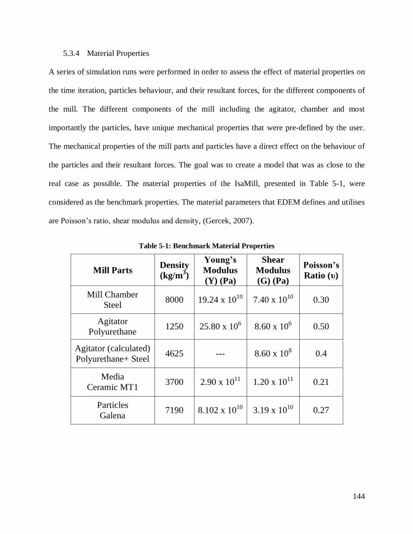
144
5.3.4 Material Properties
A series of simulation runs were performed in order to assess the effect of material properties on
the time iteration, particles behaviour, and their resultant forces, for the different components of
the mill. The different components of the mill including the agitator, chamber and most
importantly the particles, have unique mechanical properties that were pre-defined by the user.
The mechanical properties of the mill parts and particles have a direct effect on the behaviour of
the particles and their resultant forces. The goal was to create a model that was as close to the
real case as possible. The material properties of the IsaMill, presented in Table 5-1, were
considered as the benchmark properties. The material parameters that EDEM defines and utilises
are Poisson’s ratio, shear modulus and density, (Gercek, 2007).
Table 5-1: Benchmark Material Properties
Mill Parts Density
(kg/m3)
Young’s
Modulus
(Y) (Pa)
Shear
Modulus
(G) (Pa)
Poisson’s
Ratio (υ)
Mill Chamber
Steel 8000 19.24 x 10¹⁰ 7.40 x 10¹⁰ 0.30
Agitator
Polyurethane 1250 25.80 x 10⁶ 8.60 x 10⁶ 0.50
Agitator (calculated)
Polyurethane+ Steel 4625 --- 8.60 x 10⁸ 0.4
Media
Ceramic MT1 3700 2.90 x 10¹¹ 1.20 x 10¹¹ 0.21
Particles
Galena 7190 8.102 x 10¹⁰ 3.19 x 10¹⁰ 0.27

145
Iteration rate of the model was a main concern, since simulating a one second run, should not
require an enormous time to iterate. Iteration rate is defined as the number of iteration hours per
one second of simulation. The media particles were assigned the benchmark material properties
for the first simulation run, which produced a very slow run, with a very slow iteration rate (27.6
hours to simulate a one second run). A series of simulation runs were performed in order to
analyse the effect of material properties on particles behaviour and simulation iteration time. The
runs were simplified by excluding all drag forces. A simulation was performed with material
properties from the different parts of the mill, dropped to two orders of magnitude relative to
their benchmark values, where G value for media was 1.2x10⁹, agitator was 8.6x10
4, and mill
chamber was 7.4x10⁸
(simulation run a). The simulation iteration rate increased significantly to
8.78 hours for one second simulation. However, the particles did not agitate properly. Through
analysis of the forces created in the mill, it was noticed that the force values were relatively high,
compared to the other simulation runs (Table 5-2).
The next two simulation runs were performed using the material properties of the agitator and
mill chamber materials similar to the benchmark, as well as decreased the shear modulus for the
grinding media to one and two orders of magnitude, (simulation runs b, and c, consecutively).
The particle flow in the mill was closer to normal, but for simulation run b, the particles’ shear
modulus was not small enough to increase the iteration rate (20.8 hrs for each simulated second).
Simulation run c showed a better response in terms of speeding up the simulation run time. The
iteration rate of simulation run c was 7.1 hrs for each simulated second.
The fourth model run was performed with the agitator material properties defined as steel,
similar to the chamber property, which were two orders of magnitude less than the benchmark

146
values (simulation run d). The simulation iteration rate was close to that of simulation run c (6.9
hrs for each simulated second).
Other parameters that were affected by the material properties of the mill parts were the
maximum forces generated in the mill and the effective energy consumed by the particles. The
effective energy was calculated based on the ratio of output to input energy. The input energy
was calculated from the agitator torque values, and the output energy was the total kinetic and
rotational kinetic energies of the particles created in the simulation run by the agitator rotation.
As presented in Table 5-2, the steel agitator created a high value of maximum normal force,
especially in section A, and the effective energy was 7.9%, which was the highest compared to
the other simulation runs. At this point, it was noticed that the model deviated from the initial
objective, which was to create a computer model that was similar to the real case scenario. One
of the advantages of stirred mills is their inert environment for grinding, where the agitator is not
steel. The M4-IsaMill agitator used in the experiments carried out in this research was made of
steel, covered with a layer of polyurethane. The material properties of steel-covered polyurethane
were calculated. Simulation run e was then performed on an agitator shaft that was assigned the
calculated material properties of the mixed steel and polyurethane, and results were reasonable.
Finally, a similar run was conducted using the mixed steel-polyurethane agitator, and fluid drag
forces were included in the x-direction, using EDEM built-in particle body forces (simulation run
f). Simulation iteration rate was reasonable (8.3 hours for each simulated second), effective
energy percent ratio was 4%, and the force values were reasonable when compared to the
previous runs.

147
Table 5-2: Effect of Material Properties on Run Time, Forces and Energy Efficiency
Simulation Runs
Iteration
Rate
(hrs/second)
Maximum Normal
Forces
Maximum Tangential
Forces Effective
Energy
(%) A B C A B C
(a) 2 Order Mag-All
parts 8.8 4.86 2.86 1.26 1.26 0.55 0.26 3.9
(b) 1 Order Mag-
Media 20.8 1.16 0.89 0.12 0.21 0.17 0.02 3.5
(c) 2 Order Mag –
Media 7.1 1.76 1.25 0.94 0.34 0.24 0.18 3.5
(d) Steel-Agitator 6.9 2.58 2.07 1.01 0.61 0.38 0.22 7.9
(e) Steel +Poly-
Agitator 7.2 1.50 2.23 1.96 0.27 0.34 0.36 2.9
(f) Steel + Poly
Agitator & Drag
Force
8.3 2.04 1.95 1.69 0.40 0.36 0.32 4.0
5.3.5 Model Parameters
Since the model simulations were aimed at understanding the behaviour of the particles in the
mill at different operating conditions, as well as the effect of the different particle properties on
each other, the parameters were classified as fixed and variable.
5.3.5.1 Fixed Parameters
The fixed parameters were mill design, material properties, contact forces model, number of
particles and external body forces acting on the particles. The fixed parameters had to be
compromised in order to achieve a realistic simulation based on reasonable values of the iterated
parameters.

148
The fixed parameters were summarized as follows:
Mill agitator discs were circular.
Material properties input to the EDEM software are as listed in Table 5-3.
Particles and mill components interactions were coefficient of restitution, a coefficient of
static friction, and a coefficient of rolling friction. Table 5-4 lists coefficient values which
were based on similar values for similar material from the websites rocscience, 2010,
roymech, 2010, accuratus, 2010 and efunda, 2010.
Particle size was 3 mm for both media and galena.
Number of particles simulated was: media 44,775 and galena 19,407.
The contact force model was the Hertz Mindlin model.
An external body force was applied in the form of drag force (x-axis component) in the
direction of fluid flow from section A towards section C.
Table 5-3: Material Properties - Fixed Parameters
Mill Parts Density
(kg/m3)
Shear
Modulus
(G) (Pa)
Poisson’s
Ratio (υ)
Mill Chamber
Steel 8000 7.40 x 10¹⁰ 0.30
Agitator (calculated)
Polyurethane+ Steel 4625 8.60 x 10⁸ 0.4
Media
Ceramic MT1 3700 1.20 x 10⁹ 0.21
Particles
Galena 7190 3.19 x 10¹⁰ 0.27

149
Table 5-4: Particles and Mill Component Interactions
Mill Component Media Galena
COR COSF CORF COR COSF CORF
Agitator 0.4 0.2 0.01 0.35 0.35 0.01
Chamber 0.5 0.4 0.01 0.45 0.5 0.01
Media Particles 0.5 0.2 0.01 0.45 0.3 0.01
Note: COR : Coefficient of Restitution
COSF: Coefficient of Static Friction
CORF: Coefficient of Rolling Friction
5.3.5.2 Variable Parameters
The main objective of the simulation was to visualize the behaviour of the particles across the
mill length, and to quantify the forces that the different types of particles were exposed to at
different agitator speeds. The variables tested were the agitator speed and material properties,
including ceramic media and galena like minerals. The effect of the agitator speed on a single
material type in the mill, namely the ceramic media particles, were tested via a series of
simulation runs at 3 agitator speeds, 1000, 1500 and 2000 rpm. Then the effect of galena
particles on the system performance was modeled at intermediate agitator speed (1500 rpm) and
high agitator speed (2000 rpm).
The responses were quantified by varying the agitator speed and analysing the responses. It was
possible to quantify the rate at which the particles spread across the mill, as well as the type
(normal/tangential) and magnitude of forces generated at different input energies.

150
5.4 Computer Model Results
The core objective of this research was to further understand the effect of different high speed
stirred mill operating conditions (energy input via agitator speed) and the interactions between
different material types. Experimental work tested three agitator speeds (1000, 1500 and 2000
rpm), and their effect on extreme material properties (quartz and galena). For the sake of
comparison, the model runs were chosen to simulate conditions close to actual grinding
operation. To understand the effect of different simulation parameters on the modeled system,
each parameter had to be tested individually before simulating a complex system. Therefore, it
was important to start the model runs with one type of particle in the system (media particles)
and study the effect of the different agitator speeds on particle behaviour and forces generated.
Then a more complex model was generated by adding galena particles to the system and the
effect of medium and high agitator speeds were investigated. Fixed parameters for the five runs
are presented in Table 5-3 and Table 5-4.
5.4.1 Media Particles Runs
According to the particle distribution analysis shown in Figure 5-8 and Figure 5-9, the mill
reached its stable state at about the 12th
second. As a result, the simulation was run for 15
seconds to assure stable conditions were reached. The particle, forces and energy distributions
were analysed.
5.4.1.1 Particle Distribution
For the sake of comparison, the total number of particles was fixed for all simulation runs.
Particle distribution across the mill was an initial sign of system stability. Since agitator speed
dictated the energy input to the particles, it was important to evaluate the effect of the agitator
speed on stability. As shown in Figure 5-10, particle distribution across the mill was similar for

151
the three agitator speeds tested. By the 12th
second, the number of particles at the three sections
tended to approach the 15 000 particles in each section. Sections A and B started with a higher
number of particles at time zero. The number of particles decreased in section A by about 9%
and by 6% in section B, but increased by 14% in section C.

152
Figure 5-10: Particle Distribution vs. Simulation Time
(a)1000rpm, (b) 1500rpm, (c) 2000rpm
(a)
(b)
(c)

153
The initial particle distribution was 47% in section A, 39% in section B and 14% in section C. At
stable conditions (at the 12th second), the particle distribution was 38% in section A, 34% in
section B and 28% in section C. Section C had the least number of particles in the system. Fluid
flow slowed down the particle spread across the mill as shown in Figure 5-8 and Figure 5-10.
Therefore, fluid flow drag forces were incorporated in the simulation. The material properties
chosen and the number of particles distributed across the mill length were minimum at the
classifier section, bringing the model closer to the actual mill operation.
5.4.1.2 Energy Distribution
The stirred mill dynamics can be summarized as an input energy to the system via rotation of an
agitator (torque), which in turn transmits the energy to the particles in contact with the agitator.
Such particles gain kinetic and rotational kinetic energies, which are in turn transmitted to the
neighbouring particles via contacts and impacts. Hence, the energies can be summarized as input
energy via the agitator’s torque, and output energies which are the particles’ kinetic energies plus
rotational kinetic energies. Although the agitator rotation speed was pre-defined to be 1000 rpm
(5m/s), 1500 rpm (8m/s) and 2000 rpm (10m/s), the lifting and agitation of the particles created
resistance, which in turn changed the agitator’s torque values per time step. In order to trace the
effect of lifting and agitation on torque values, the agitator torque value was saved after every
iteration interval, as well as total kinetic energies and rotational kinetic energies of all the
particles for each section in the mill (A, B and C). Energy values were exported to a spread sheet
for analysis. Input energy from the agitator was calculated using the torque values, as per
Equation 5-12. Output energies were the sum of all the kinetic and rotational kinetic energies for
all the particles, as per sections A, B and C. Output versus input energies were plotted, and the
slopes of the lines were the effective energy ratio in the mill, as shown in Figure 5-11.

154
Where:
EI: input energy
T: torque
rpm: revolution per minute
t: time
Figure 5-11: Output vs. Input Energies for Media Runs
(a)1000rpm, (b) 1500rpm, (c) 2000rpm, (d) Full Mill
(a) (b)
(c) (d)
Equation 5-12

155
The energy distribution differed in the three sections of the mill according to the agitator speed.
Section C was exposed to the least energy for the three agitator speeds. Section A and B had
similar energy distribution throughout the simulation time at 1500 rpm, Figure 5-11(b). The
sections also had similar energy distributions up to an input energy of 400 J for the 2000 rpm
(Figure 5-11(c)). Beyond an input energy of 400 J at 2000 rpm, section B showed a steeper slope
than section A (Figure 5-11(c)), which implied that the same input energy in section B was better
utilized by the particles than that in section A. The commencement of the run showed similar
particle behaviour in sections A and B at 1000 rpm (Figure 5-11(a)). The overall effective energy
percent ratio (ratio of output to input) for the three agitator speeds were 4.9% for 1000 rpm, 4%
for 1500 rpm and 4.4% for 2000 rpm as in Figure 5-11(d). The experimental and theoretical
(computer model) effective energies could not be compared directly, since the energies
encountered in the actual mill had complex parameters that were not addressed by the computer
model. The dynamics of a continuous flow of slurry through the mill, the actual particle breakage
versus time, the particle size distribution in the slurry mix, were all parameters that were not
considered in this research.
To evaluate the energy balance across the mill, effective energy ratio was plotted versus
simulation time Figure 5-12. The effective energy ratio consistently increased in section C at a
higher rate for the higher agitator speed. For sections A and B during the first two seconds of the
run, the mill experienced a disturbance at the three agitator speeds. Then the effective energy
ratio stabilized according to the agitator speed. The effective energy ratio stabilized when it did
not change with time, which implied that the particles gained their inertia relative to the mill
agitator rotation, and that the effect of lifting and falling of the particles versus energy
consumption during the agitation was not changing with time. The effective energy ratio in

156
sections A and B coincided after the first 2 seconds at 2000 rpm, they converged at the 8th second
at 1500 rpm, and they were almost parallel at 1000 rpm.
The effective energy ratio was highest at the lowest agitator speed (1000 rpm), followed by the
2000 rpm, and the lowest effective energy ratio was at the 1500 rpm. The results could be
explained by particles dynamic in the mill relative to the agitator torque and individual particles’
kinetic flow. The agitator torque was directly affected by the number of particles resting on the
agitator, which in turn affected the center of mass of the particles that the agitator was lifting.
Cumulative energy trends were further evaluated.
Figure 5-12: Media Effective Energy Ratio vs. Simulation Time
0.00
0.01
0.02
0.03
0.04
0.05
0.06
0.07
0 2 4 6 8 10 12 14 16
Effectiv
e E
nerg
y R
atio
Time (sec)
1000 RPM
Section A
Section B
Section C
0.00
0.01
0.02
0.03
0.04
0.05
0.06
0.07
0 2 4 6 8 10 12 14 16
Effectiv
e E
nergy
Ra
tio
Time (sec)
1500 RPM
Section A
Section B
Section C
0.00
0.01
0.02
0.03
0.04
0.05
0.06
0.07
0 2 4 6 8 10 12 14 16
Effecti
ve E
nerg
y R
ati
o
Time (sec)
2000 RPM
Section A
Section B
Section C
0.00
0.02
0.04
0.06
0.08
0.10
0.12
0.14
0 2 4 6 8 10 12 14 16
Effecti
ve E
nerg
y R
ati
o
Time (sec)
Full Mill Energy Efficiency
1000RPM
1500RPM
2000RPM
(a) (b)
(c) (d)

157
The cumulative energy trends did not follow the agitator speed. The intermediate agitator speed,
1500 rpm, had the lowest effective energy ratio, and the lowest agitator speed had the highest as
shown in Figure 5-12 (d). Therefore, instantaneous torque, input and output energies were further
investigated. The torque trend showed similarity for the three agitator speeds as presented in
Figure 5-13. The standard deviation of the average torque among the three agitator speeds was
only 0.0081, which showed that the torque was quite constant for the three agitator speeds. This
observation contradicted the expected torque values relative to the agitator speed. The simple
equation for torque was the tangential force multiplied by the radius on which the force was
acting. The torque on the agitator, calculated by EDEM, was the tangential contact force,
multiplied by the distance from the center of mass of the particles resting on the agitator, to the
contact point. Therefore, the amount of stationary particles on the agitator dictated the distance to
be multiplied by the tangential contact force, which in turn affected the torque value during
agitation. The average number of particles in contact with the agitator was inversely proportional
to the agitator speeds. The number of particles in contact with the agitator was 508, 412 and 387
at agitator speeds 1000, 1500 and 2000 rpm, respectively. This implied that the torque values
should have an order similar to the number of contact particles, where the lowest agitator speed
should posses the highest torque value and the highest agitator speed should have the highest
torque values.
In order to translate the torque into input energy, the torque values were multiplied by the
agitator speed, which created the proportional differences of the input energy curves, relative to
the agitator speeds as shown in Figure 5-14(a). On the other hand, the output energies, kinetic
and rotational energies were individually calculated by EDEM based on the particle velocities
and rotational velocities. The proportional differences of the output energy curves, relative to the

158
agitator speeds, as shown in Figure 5-14(b) were similar to the input energy, Figure 5-14(a). The
results agreed with the empirical power equation of Gao’s et al. (1996), (Equation 2-4). This
equation related the mill power consumption to the agitator speed to the power of 1.429,
where . Since power is the product of torque and agitator speed ( ), then with
direct substitution, ( , the torque would be directly proportional to the power of
0.429 ( ). This implied that the effect of the agitator speed (N) on the power/energy
was more significant when compared to its effect on torque, which explained the insignificant
response of the torque to the agitator speed when compared to the power.
Figure 5-13: Torque vs. Simulation Time
Figure 5-14: Instantaneous Energy vs. Time Simulation, a) Input Energy, b) Output Energy
0.00
0.05
0.10
0.15
0.20
0.25
0.30
0.35
0.40
0 5 10 15
To
rqu
e (
Nm
)
Time (sec)
15 per. Mov. Avg. (1000) 15 per. Mov. Avg. (1500) 15 per. Mov. Avg. (2000)
0.0
1.0
2.0
3.0
4.0
5.0
6.0
7.0
8.0
0 5 10 15
Inpu
t E
nerg
y
Time (sec)
15 per. Mov. Avg. (1000) 15 per. Mov. Avg. (1500) 15 per. Mov. Avg. (2000)
0.00
0.05
0.10
0.15
0.20
0.25
0 5 10 15
Outp
ut
Energ
y
Time (sec)
15 per. Mov. Avg. (1000) 15 per. Mov. Avg. (1500) 15 per. Mov. Avg. (2000)
(a) (b)

159
Despite the fact that the model agreed with other empirical mathematical models that related the
power to agitator speed (Gao’s et al., 1996), the relationship between energy utilization and types
of forces was not entirely understood. Energy input was utilised as friction, impact, linear and
rolling velocities, tangential forces and normal forces. From the effective energy percent ratio
plots for the three agitator speeds in Figure 5-11(d), it could be deduced that at a speed of 1500
rpm, the energy input was used differently than at other agitator speeds. EDEM would track and
save the tangential and normal forces, which were then exported for further analysis.
5.4.1.3 Forces Distribution
Stirred milling exposes the particles to both fracture and attrition. Fracture is due to impact and
compressive forces, which could be translated using a computer model into the normal
component of the forces applied on the particles. Attrition breakage is due to abrasion, which
could be identified in a computer model as the tangential component of the forces applied on the
particles. Maximum normal and tangential forces, for each time step, and at each section in the
mill (sections A, B and C) were exported, and their averages were calculated over the total
simulation time. The highest normal and tangential forces occurred primarily in section A, due to
the highest number of particles in this section. A higher agitator speed generated consistent
higher normal forces in all three sections of the mill. Tangential force values were not
significantly different between the three agitator speeds; however, there was a trend where the
agitator speed of 1500 rpm produced higher tangential forces than the 1000 and 2000 rpm. The
magnitude of the average normal forces were approximately 6.8 and 7.3 times more than the
tangential forces for 1000 and 2000 rpm, respectively, while normal forces for the 1500 rpm
were 5.2 times more than the tangential forces. Detailed force values are shown in Table 5-5.

160
Table 5-5 : Maximum Normal and Tangential Forces
The results indicated that an agitator speed of 1500 rpm would expose the particles to about 26%
more tangential forces than normal forces, compared to the 1000 and 2000 rpm. This indicated
that more abrasion was likely occurring at 1500 rpm than the lower or higher agitator speeds.
Since the energy input to the mill was not fully utilized by the particles at 1500 rpm (less energy
efficiency), the particle dynamics at 1500 rpm were different than at the other agitator speeds. As
for the 1000 and 2000 rpm, the dominant forces were the compressive forces, which would be
translated to fracture breakages rather than abrasion in actual grinding operation.
5.4.1.4 Average Force Distribution
The force distribution across the mill was assessed qualitatively via snap shot images at
instantaneous times. The images were along section A-A of the mill or across the center between
the discs, section B-B, as shown in Figure 5-15(a) and (b).
A B C A B C
1000 2.0 1.6 0.8 0.3 0.2 0.1
1500 2.3 1.9 1.2 0.5 0.4 0.2
2000 2.7 2.3 1.7 0.4 0.3 0.2
Maximum Normal Forces (N) Maximum Tangential Forces (N)RPM
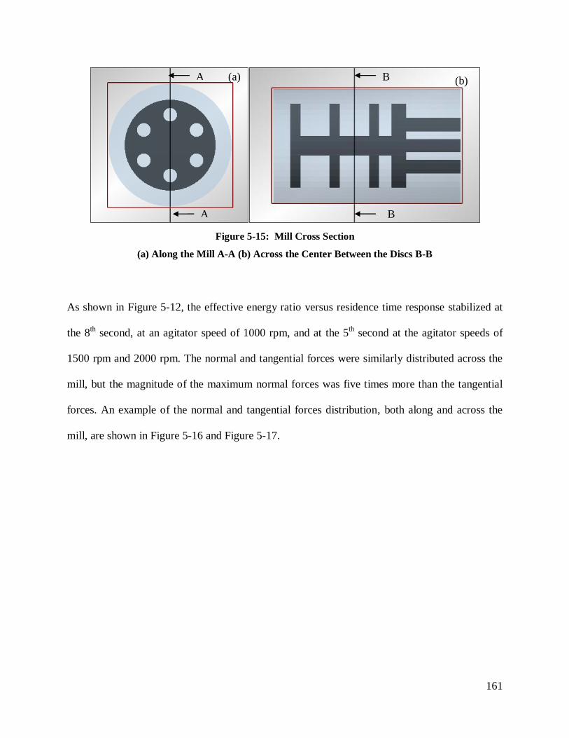
161
Figure 5-15: Mill Cross Section
(a) Along the Mill A-A (b) Across the Center Between the Discs B-B
As shown in Figure 5-12, the effective energy ratio versus residence time response stabilized at
the 8th
second, at an agitator speed of 1000 rpm, and at the 5th second at the agitator speeds of
1500 rpm and 2000 rpm. The normal and tangential forces were similarly distributed across the
mill, but the magnitude of the maximum normal forces was five times more than the tangential
forces. An example of the normal and tangential forces distribution, both along and across the
mill, are shown in Figure 5-16 and Figure 5-17.
A
A
B
B
(a) (b)

162
Figure 5-16: (a) Normal and (b) Tangential Forces Distribution in Section A-A for 1000 rpm run
(a)
(b)

163
Figure 5-17: (a) Normal and (b) Tangential Forces Distribution in Section B-B for 1000 rpm
(a)
Lifting
Section
(b)

164
The effect of the agitator speed on normal force distribution is presented in Table 5-6. The higher
agitator speed would drive the particles out and away from the agitator towards the inner wall of
the mill chamber, via centrifugal acceleration forces, as shown in section A-A. The forces were
higher in the middle section between the discs at the medium agitator speed, 1500 rpm. The
radial distribution of the normal forces, section B-B, was similar for the three agitator speeds.
The forces in the lifting section possessed average values of 3x10⁻³
N normal forces and 6x10⁻⁴
N
tangential force, whereas the highest force values were closer to the inner chamber wall, with
different intensities according to the agitator speed. The force distribution dissipated at the
classifier section, but did not completely disappear. In other words, grinding occurred throughout
the mill, but the highest grinding forces were between the discs.

165
Table 5-6: Normal Forces Distribution Across the Mill at 1000, 1500 and 2000 rpm Agitator Speed
1000 rpm 1500 rpm 2000 rpm
Section
A-A
Section
B-B

166
5.4.2 Galena and Media Particles Runs
Since this study incorporated the effect of different material properties on the mill performance,
19,407 particles similar to galena properties were added to the system. The total number of
media plus galena particles in the system totalled 64,182 particles. Accordingly, the iteration
time of the simulation run increased drastically, due to the increased number of particles in the
system. Therefore, the simulation runs were shortened to 5 seconds instead of 15 seconds, and
only 2 agitator speeds were tested, 1500 and 2000 rpm.
5.4.2.1 Particle Distribution
The particle distribution across the mill was evaluated separately, based on the type of particles.
After running the model on the mixed media plus galena, the media particles were distributed
across the three sections of the mill with the same distribution as the run with only media. The
spread of the particles across the three sections was faster with the presence of galena in the
system compared to media-only runs (Figure 5-18, a, c). For the galena run at 1500 rpm, the
number of particles in section A did not change much by the 5th
second. The number of galena
particles at the same agitator speed in sections B and C were equal by the 2nd
second, with
60 000 particles in each section, (Figure 5-18 b). At 2000 rpm (Figure 5-18d), the number of
galena particles in section C was greater than in section B.

167
Figure 5-18: Number of Particles Distribution Across the Mill:
(a) Media distribution at 1500 rpm;
(b) Galena distribution at 1500 rpm;
(c) Media distribution at 2000 rpm;
(d) Galena distribution at 2000 rpm
0
5000
10000
15000
20000
25000
0 1 2 3 4 5
Nu
mb
er o
f P
arti
cle
s
Time (sec)
G1500 RPM - Media
A
B
C
0
2000
4000
6000
8000
10000
0 1 2 3 4 5
Nu
mb
er o
f P
arti
cle
s
Time (sec)
G1500 RPM - Galena
A
B
C
0
5000
10000
15000
20000
25000
0 1 2 3 4 5
Nu
mb
er o
f P
arti
cle
s
Time (sec)
G2000 RPM - Media
A
B
C
0
2000
4000
6000
8000
10000
0 1 2 3 4 5
Nu
mb
er o
f P
arti
cle
s
Time (sec)
G2000 RPM - Galena
A
B
C
(a) (b)
(c) (d)
(a)

168
Figure 5-19: Initial Particle Distribution at Time Zero: (a) Radial Direction, section B-B; (b) Linear
Direction, section A-A, (c) Isometric corss section
Visual evaluation of the galena particle mixing showed that the distribution became more
homogenous by the end of the 5th
second. It was presumed that 5 seconds were not enough for
complete homogenization and proper mixing of the galena and media particles. Agitator speed
did not show a major effect on mixing and homogenizing the two types of particles (Table 5-7
and Table 5-8).
(a) (b)
(c)
Galena
Media Media

169
Table 5-7: Mixed Media and Galena Particles Distribution at 1500 rpm
Simulation
Time
Radial
Section B-B
Linear
Section A-A Isometric
1st
Second
1500 rpm
2.5th Second
1500 rpm
5th Second
1500 rpm

170
Table 5-8: Mixed Media and Galena Particles Distribution at 2000 rpm
Simulation
Time 1
st Second 2.5
th Second 5
th Second
2000 rpm
5.4.2.2 Maximum Forces Distribution
The maximum normal and tangential forces over the 5 second simulation run were exported for
media and galena particles for agitator speeds tested, 1500 and 2000 rpm. Galena particles
possessed the highest force values for both speeds. The detailed force distribution is shown in
Table 5-9. Both the tangential and normal forces on the galena particles were higher than on the
media particles. The average tangential forces of the galena particles were 24% and 31% higher
than media particles for the agitator speeds 1500 and 2000 rpm, respectively. The average
normal forces of the galena particles were 4% and 8% higher than the media particles for the
agitator speeds 1500 and 2000 rpm, respectively.
The agitator speed had a direct effect on the forces encountered by the particles, based on the
particle type. By increasing the agitator speed, the average increase of the tangential forces of the
galena particles, relative to the media particles, was 24%. On the other hand, the average
increase of the normal forces of the galena particles, relative to the media particles, was 50%.
The data implied that the major breakage mode of galena particles was abrasion, since tangential
forces were dominant. By increasing the agitator speed, the average increase of the normal forces

171
on the galena particles relative to the media particles was almost double. The data agreed with
the morphology results, where the galena concentrate breakage mode was dominantly abrasion at
low agitator speed, and turned into fracture at a higher agitator speed.
Table 5-9: Maximum Normal and Tangential Forces Distribution
5.4.2.3 Average Force Distribution
Quantitative analysis of the force distribution across the mill showed that grinding occurred
throughout the mill, and that it increased at the classifier section. The media-only runs showed
no grinding occurring at the classifier section for both agitator speeds (1500 and 2000 rpm), as
shown in Figure 5-20 and Figure 5-21. The classifier section was populated by a higher number
of particles, especially galena, by the 2nd
second, which in turn created more interaction between
the particles. The galena particles were heavier than the media, which created a higher inertia
once the particles were put in motion. The inertia was in addition to the overall higher number of
particles in the mill that affected the particle kinematics within the same volume of the mill
chamber. At high agitator speed (2000 rpm) the particles spread towards the inner walls of the
mill chamber with high values of normal forces, (Figure 5-21 a). The highest values of normal
forces were under the agitator discs, and the particles were cascading closer to the agitator shaft
A B C A B C
1500 Media 4.4 3.5 4.7 1.1 0.9 1.1
1500 Galena 4.7 4.1 4.3 1.6 1.4 1.2
2000 Media 4.5 4.4 4.1 1.0 1.1 1.0
2000 Galena 5.4 3.7 5.0 1.8 1.1 1.5
Maximum Normal Forces (N) Maximum Tangential Forces (N)RPM

172
than was the case with media runs, as shown in Figure 5-20b, Figure 5-21b and section B-B in
Table 5-6.
Figure 5-20: Normal Forces Distribution at 1500 rpm (a) Section A-A; (b) Section B-B
Figure 5-21: Normal Forces Distribution at 2000 rpm (a) Section A-A; (b) Section B-B
5.5 Conclusion
A computer simulation of the Isa-Mill was included in this research in order to further
understand the forces, energies and particle distribution across the mill at different operating
conditions, as well as the interaction of the particles relative to each other using the Discrete
Element Method.
(a)
(a)
(b)
(b)
173
Almost all computer models require a degree of compromise and deviation from an actual
system, due to the intensive computational requirements of such models. It was believed that the
parameters chosen for the basic simulation runs were the most appropriate based on the
computational abilities of the computer. The parameters chosen were based on a series of
simulation runs which evaluated each parameter individually. The parameter levels selected
brought the model close to a real IsaMill operation.
The simulation runs had very good association with the particle breakage mechanisms observed
in the morphology study. The types of forces encountered in the model were correlated to the
type of particle breakages presented by the morphology analysis.
It was observed that the agitator speed 1500 rpm exposed the media particles to 26% more
tangential forces than normal forces when compared to agitator speeds of 1000 and 2000 rpm.
This observation was similar to morphology results for quartz, where abrasion was dominant at
the medium agitator speed of 1500 rpm. On the other hand, the dominant forces at 1000 and
2000 rpm agitator speeds were normal, compressive forces, which were equivalent to fracture
breakage in an actual grinding process. It was also concluded that the media particle dynamics at
1500 rpm were different, as the effective energy ratio was the lowest at this agitator speed, when
compared with 1000 and 2000 rpm.
In order to understand the effect of the different particle properties on the forces generated and
their dynamics in the mill, particles whose properties were similar to galena properties were
added to the system. However, due to the vast number of particles in the system which were
drastically hindering the simulation time iteration, media and galena runs were limited to 5
seconds. It was observed that the media particle distribution across the mill over the 5 seconds

174
was similar to the runs with only media particles in the system. The galena particles behaved
differently. The number of galena particles in the first section of the mill, section A, slightly
decreased as time elapsed. Whereas for the medium agitator speed (1500 rpm) the particles in the
middle and classifier sections, sections B and C, increased up to an equal number of particles,
60 000, by the 2nd
second. At the high agitator speed (2000 rpm), the number of particles in
section C was slightly more than the number of particles in section B. Visual examination of
media and galena particles mixing and homogenizing showed that five seconds were not quite
enough time in order to reach a stable, homogenized system.
On the other hand, quantitative analysis of the media and galena particle forces provided some
insight into the type of breakage that the different types of particles were exposed to in the mill at
different agitator speeds. The data agreed with the morphology results, that the major breakage
mode of galena particles was abrasion, since tangential forces were dominant. Morphology
results also showed that by increasing the agitator speed, a fracture breakage mode started to
show, and this breakage along grain boundaries. Those results complied with the model findings,
which demonstrated that at the higher agitator speed, the normal forces of the galena particles,
relative to the media particles, increased by 50%. Normal forces were translated into
compressive forces that would consequently impose fracture breakage along the grain
boundaries.
The coherent findings of the DEM model, with the equivalent observations of the morphology
analysis, contributed to the understanding of the particle breakage mode and mechanism. Thus, a
DEM model could be used to predict types of particle breakages in stirred milling, based on the
material properties of the particles and mill operating conditions.

175
6. Conclusions and Recommendations
6.1 Conclusions
The major objective of this research was to gain a comprehensive understanding of how
operating parameters would affect particle breakage mechanisms in stirred mills. In order to
achieve the objective, state of the art researches performed on stirred mills were reviewed. It was
recognised that the operation and performance of these mills was only empirically understood.
Breakage modes of the particles under different grinding mechanisms were morphologically
analysed. The literature was reviewed in order to summarize the relationship between breakage
mode and surface texture (morphology features). The effect of different operating conditions and
different material properties on grinding performance was analysed via particle size reduction
analysis and energy consumption.
Experimental results were supported by discrete element modeling (DEM). None of the models
performed to date related the effect of different particle properties on each other. The computer
simulation models performed on the IsaMill were over simplified. The effect of the media
classifier, and the classifier on the particle flow and distribution were not investigated. The
computer model in this study was designed to be as close as possible to the real case scenario, so
that the forces and energy distributions across the mill were quantitatively analysed.

176
The conclusions of the experimental work can be summarized as follows:
6.1.1 Experimental Work
The parameters addressed in the experimental work were material properties, machine
input energy, in the form of different agitator speeds, and residence time effect on
breakage behaviour.
The materials chosen for the set of experiments were quartz and galena concentrate that
were extreme in their hardness values as well as their specific gravity. The other two
materials chosen were a mixed sample of galena and quartz with a ratio of 1:6, and a
similar but locked lead-zinc ore sample from the SAG discharge of Red Dog mine.
The machine input energy was defined by three agitator speeds which were 1000, 1500
and 2000 rpm.
The residence time effect on grinding was studied by circulating the material into the
mill five times, so that the same particles would be exposed to the same grinding
mechanism for a longer time. The flow rate was set at 3.5 L/min, which was the highest
flow rate the machine could handle.
Material type had a major effect on particle size distribution and size reduction at the
three agitator speeds evaluated.
Quartz did not break efficiently at the 1000 rpm agitator speed, which indicated that
there was a minimum energy input required to initiate and break the quartz particles.
On the other hand, the 1000 rpm was enough for the galena to break. The extreme
agitator speed of 2000 rpm, broke the galena particles down to their grinding limit after
the first pass through the mill.

177
The effect of the quartz breakage mechanism was dominant over the galena, due to the
higher content of quartz compared to galena, ratio of 6:1.
The initial breakage rate of the 4 materials tested increased linearly with the increase of
the agitator speed. However, breakage rates were almost one order of magnitude higher
for the soft minerals than the hard minerals. Average breakages were directly affected
by how close the particle sizes were to their grinding limit. Breakage rate decreased
once it reached the grinding limit of the material.
The breakage rate was linear for most of the grinds, except for the quartz at 2000 rpm,
the galena concentrate at 1000 rpm, the mix at 2000 rpm and the lead-zinc ore sample at
1500 and 2000 rpm. At these agitator speeds an exponential breakage rate trend was
revealed. This observation indicated that quartz, the harder mineral would break faster
at the higher agitator speed, whereas galena, the soft mineral, would break faster at a
lower agitator speed. The breakage mechanism of the mix quartz and galena sample
followed the harder mineral mechanism rather than the softer mineral. As for the lead-
zinc ore sample breakage rate, it was faster at the 1500 and 2000 rpm, which indicated
that it had a high content of hard minerals, as well as a reasonable amount of soft
minerals. The hard minerals lead to fast breakage rate at high agitator speed and the soft
minerals lead to fast breakage rate at intermediate agitator speed.
Energy consumption was evaluated using the typical signature plots. There was some
overlap in the energy required versus targeted size between the different agitator speeds;
however, the overlap was not consistent. The analysis also revealed that the data fit
differently to the power and exponential equations, based on the type of material and
agitator speed selected for grinding.

178
The agitator speed has a higher effect on the mill’s effective energy ratio than the type
of mineral it is grinding. The higher the agitator speed, the better use of the energy
input to the mill during the grinding process.
The amount of energy required to break one micron was directly affected by the type of
material being ground. Soft minerals required less energy per micron at all agitator
speeds. Thus, the softer minerals would break faster at lower agitator speed than harder
minerals and vice versa.
6.1.2 Morphology
Morphology analysis assists in understanding the breakage behaviour of the different material
properties at different stress intensity inputs, in the form of the agitator speeds. Results from this
research demonstrated that there was a potential to understand grinding versus liberation, beyond
the obvious fact that the smaller the particles, the more the minerals will be liberated.
The major morphological features analysed were the surface roughness, roundness and
elongation of the particles. Surface roughness dictates the type of breakage, whether it is
along the grain boundaries or across them. The breakage along the grain boundaries
should create rougher surfaces and less circular particles.
Roughness values were assessed using Clemex software, and results were biased to
smooth counts. Accordingly, a manual point count method was developed and tested.
Despite the fact that there was about 6% difference between counters, based on their
judgement of the degree of roughness of the particles, the trends of the data of the
manual point count and Clemex software results were similar and correlated.
Initial breakage results according to the Clemex analysis coincided with the manual
point counting and stacked charts. The galena concentrate had a trend of fracture

179
breakage along grain boundaries, at the higher agitator speed of 2000 rpm, whereas
quartz had a trend of abrasion breakage, across grain boundaries, at the same agitator
speed. This suggested that if the target was to liberate minerals similar to galena, then a
higher agitator speed would be recommended.
The effect of residence time reflected a similar trend for Clemex analysis and manual
point counting, using Pearson’s time correlation. Increasing residence time promoted
abrasion breakage (transgranular breakage) for both galena concentrate and quartz.
Visual observations and trends counts of rough (R4+R5) and smooth (R1+R2)
particles showed that stirred mills broke the particles via both abrasion and fracture.
The overall trends for both types of materials (quartz, and galena concentrate)
demonstrated that the amount of rough particles was always higher than smooth
particles. This observation could be interpreted as fracture being the breakage
mechanism that was dominant in the grinding system, along with some abrasion. This
hypothesis was built on the observation that the particles size decreased during the
grinding process, as per the PSD analysis. Therefore, in spite of the fact that the size
fractions counted were similar, they were the progeny of coarser fractions. The trends
proved that an abrasion breakage mechanism increased with time and existed in the
stirred milling process, but that fracture was equally present, if not dominant during
initial breakages, and for fine fractions.
If the target was to liberate, soft mineral such as galena, then higher agitator speed as
well as short residence time in the mill would be recommended and vice versa for hard
minerals.

180
Flow dynamics in the mill were not exclusively dependent on the hardness of the
mineral. Liberation analysis of the lead-zinc ore sample showed that pyrite and quartz
were close in hardness values. Mohs hardness values were 6.5 and 7, respectively.
Liberation dependent on the specific gravity of the minerals, which dictated the flow
dynamics in the mill and surface energy per unit mass.
It was learned from the morphology analysis that minerals, similar to galena properties,
would break faster at lower agitator speeds. However, breakage would be achieved via
abrasion. In order to impose intergranular breakage on minerals similar to galena
properties, a higher agitator speed and shorter residence time would be recommended.
In other words, mode of breakage should be a priority over breakage rate in order to
produce liberated particles.
6.1.3 Computer Model
Discrete Element Modeling was utilized in this study to further understand the forces, energies
and particle distributions across the mill at different operating conditions.
Computer modeling is a data intensive computing system which demands compromise
and deviation from the parameters of an actual system. To create a model close to a real
IsaMill, a series of simulation runs were performed in order to evaluate each parameter
individually. The parameters were:
- The number of particles,
- Material properties of the mill and of the particles,
- Presence versus absence of fluid flow.

181
The computer model simulation runs produced a very good association between the
particle breakage mechanisms observed by the morphology results, and the types of
forces encountered in the model.
A summary of the observations from the simulation runs were as follows:
- The medium agitator speed, 1500 rpm, exposed the media particles to 26% more
tangential forces than normal forces, when compared to agitator speeds of 1000
and 2000 rpm. This observation was similar to morphology results for quartz,
where abrasion was dominant at the medium agitator speed, 1500 rpm. On the
other hand, the agitator speeds of 1000 and 2000 rpm as dominant forces were
normal, compressive forces.
- It was also concluded that the dynamics of the media particles in the mill at 1500
rpm were different than that of the 1000 and 2000 rpm agitator speeds, since the
effective energy ratio was the lowest at 1500 rpm agitator speed.
Particles with properties similar to galena were added to the system to understand the
effect of the different particle properties on the forces generated, and their dynamics in
the mill. However, due to the increased number of particles in the system which
drastically hindered the simulation time iteration, the mixed particles, media and galena,
runs were limited to 5 seconds. The galena and media particle simulation results can be
summarized as follows:
- Media particle distributions across the mill over the 5 seconds were similar to the
runs with only media particles in the system. Galena particle distributions
behaved differently. The number of Galena particles in the first section of the mill,
section A, slightly decreased as time elapsed for the both agitator speeds, 1500
182
and 2000 rpm. The middle and classifier sections (B and C) both had 60 000
particles at 1500 rpm agitator speed by the 2nd
second, but the number of particles
increased in section C, compared to section B at the 2000 rpm agitator speed.
- Visual examination of media and galena particles mixing and homogenizing
showed that the five seconds were not enough to reach a stable, homogenized
system.
- The quantitative analysis of the type of forces generated by the media and galena
particles agreed with the morphology results. The major breakage mode for galena
was abrasion, since tangential forces were dominant. Morphology results also
showed that by increasing the agitator speed, fracture breakage mode, that is
breakage along grain boundaries, started to come into view. Those results
complied with the model findings, which demonstrated that the higher agitator
speeds increased the average increase of the normal forces of the galena particles
relative to the media particles, by 50%. Normal forces were translated into
compressive forces that would consequently impose fracture breakage, along the
grain boundaries.
- The coherent findings of the DEM model, along with the equivalent observations
of the morphology analysis, contributed to the understanding of the particle
breakage mode and mechanism. Thus, a DEM model could be used to predict
types of particle breakages in stirred milling, based on the particle material
properties and mill operating conditions.

183
6.2 Recommendations
This work was a comprehensive study on the stirred mill operation and particle breakage. Some
of the tools utilized in this study were new to the industry, such as the morphology analysis, and
other tools were extensively used, such as the computer modeling. However, most of the
computer models were analysed qualitatively, rather than quantitatively. Also, the correlation
between the experimental and the computer models were rarely addressed in literature.
Nevertheless, more work still needs to be performed on morphology, as well as the quantitative
computing models is needed in order to fully understand the mill performance and operation so
that knowledgeable operating conditions could be employed rather than applying empirical data.
Recommendations for further work are summarized as follows:
6.2.1 Experimental and Morphology
Perform a similar series of grinding experiments using multi-size grinding media to
reach a real grinding limit of the material in question.
Further investigation on the actual material properties that cause different types of
breakage, fracture, or abrasion, such as hardness, specific gravity and crystal structure
of the mineral.
A complete, detailed liberation/morphology analysis for all size fractions, so that a
proper liberation balance may be performed.
Additional work on the 3D liberation analysis versus the conventional method, in order
to generate a correlation that can be used for a quick, and inexpensive, preliminary ore
characterization.

184
6.2.2 Computer Modeling
Invest in a more powerful computer that can handle larger number of particles and
longer simulation times, in order to bring the model closer to a real stirred mill
performance.
Couple the model to CFD (Computer Fluid Dynamics) software and run a similar set of
models, in order to understand and visualize the performance of the particles in the mill
quantitatively as well as qualitatively.
Add irregular shaped particles to the system and trace them through the mill at different
agitator speeds.

185
References
accuratus, MT1 grinding media. Retrieved April, 14, 2009, from
http://accuratus.com/alumox.html
Ahmed, M. M. (2010). Effect of comminution on particle shape and surface roughness and their
relation to flotation process. International Journal of Mineral Processing, 94(3-4), 180-191.
Alex, T. C., Kumar, R., Roy, S. K., & Mehrotra, S. P. (2008). Stirred bead mill grinding of
gibbsite: Surface and morphological changes. Advanced Powder Technology, 19(5), 483-
491.
Barley, R. W., Conway-Baker, J., Pascoe, R. D., Kostuch, J., McLoughlin, B., & Parker, D. J.
(2004). Measurement of the motion of grinding media in a vertically stirred mill using
positron emission particle tracking (PEPT) part II. Minerals Engineering, 17(11-12), 1179-
1187.
Becker, M., Kwade, A., & Schwedes, J. (2001). Stress intensity in stirred media mills and its
effect on specific energy requirement. International Journal of Mineral Processing, 61(3),
189-208.
Blecher, L., Kwade, A., & Schwedes, J. (1996). Motion and stress intensity of grinding beads in
a stirred media mill. part 1: Energy density distribution and motion of single grinding beads.
Powder Technology, 86(1), 59-68.
Botin, J. A. (2009). Sustainable management of mining operations. SME: Society of Mining,
Metallurgy and Exploration, Inc.

186
Celep, O., Aslan, N., Alp, İ., & Taşdemir, G. (2011). Optimization of some parameters of stirred
mill for ultra-fine grinding of refractory Au/Ag ores. Powder Technology, In Press, 208 (1),
121-127
Celik, I. B., & Oner, M. (2006). The influence of grinding mechanism on the liberation
characteristics of clinker minerals. Cement and Concrete Research, 36(3), 422-427.
Cleary, P. W., Sinnott, M., & Morrison, R. (2006). Analysis of stirred mill performance using
DEM simulation: Part 2 – coherent flow structures, liner stress and wear, mixing and
transport. Minerals Engineering, 19(15), 1551-1572.
Clemex Technologies Inc., User Guide, Vision PE & Vision Lite 6.0 , 2009.
Coefficient of restitution. Retrieved September, 14, 2010, from
http://www.rocscience.com/downloads/rocfall/webhelp/rocfall/Coefficient_of_Restitution.htm
Conway-Baker, J., Barley, R. W., Williams, R. A., Jia, X., Kostuch, J., McLoughlin, B., et al.
(2002). Measurement of the motion of grinding media in a vertically stirred mill using
positron emission particle tracking (PEPT). Minerals Engineering, 15(1-2), 53-59.
Cundall, P, Stack, O, (1979), Discrete numerical model for granular assemblies.
Geotechnique,(29), 47.
Datta, A., & Rajamani, R. K. (2002). A direct approach of modeling batch grinding in ball mills
using population balance principles and impact energy distribution. International Journal of
Mineral Processing, 64(4), 181-200.

187
Dishman, K., Doolin, P., & Hoffman, J. (1993). Comparison of particle size of cracking catalyst
determined by laser light scattering and dry sieve methods. Ind. Eng. Chem, 32, 1457-1463.
Donskoi, E., Suthers, S. P., Fradd, S. B., Young, J. M., Campbell, J. J., Raynlyn, T. D., et al.
(2007). Utilization of optical image analysis and automatic texture classification for iron ore
particle characterisation. Minerals Engineering, 20(5), 461-471.
efunda, Stainless steel properties. Retrieved April, 14, 2009, from
http://www.efunda.com/materials/alloys/stainless_steels/show_stainless.cfm?ID=AISI_Typ
e_316&prop=all&Page_Title=AISI%20Type%20316
Farag, M. (1989). Selection of materials and manufacturing processes for engineering design.
UK: Prentice Hall.
Farber, B. Y., Knopjes, L., & Bedesi, N. (2009). Advances in ceramic media for high energy
milling applications. Minerals Engineering, 22(7-8), 704-709.
Frances, C., Le Bolay, N., Belaroui, K., & Pons, M. N. (2001). Particle morphology of ground
gibbsite in different grinding environments. International Journal of Mineral Processing,
61(1), 41-56.
Freedman, D., Pisani, R and Purves, R. (1998), Statistics, Third Edition, W. W. Norton &
Company Inc.
Gabriel, B. (1985). In American Society of Metals (Ed.), SEM: A user's manual for material
science. Ohio: Metals Park.

188
Gao, M., & Holmes, R. (2007). Developments in fine and ultrafine grinding technologies for the
minerals industry. CSIRO Minerals, Australia, the Institute of Materials , Minerals, and
Mining (IOM3), 2007., , October 15, 2010.
Gao, M., Forssberg, K. S. E., & Weller, K. R. (1996). Power predictions for a pilot scale stirred
ball mill. International Journal of Mineral Processing, 44-45, 641-652.
Gao, M., & Forssberg, E. (1993). A study on the effect of parameters in stirred ball milling.
International Journal of Mineral Processing, 37(1-2), 45-59.
Gercek, H. (2007). Poisson's ratio values for rocks. International Journal of Rock Mechanics and
Mining Sciences, 44(1), 1-13.
Gers, R., Climent, E., Legendre, D., Anne-Archard, D., & Frances, C. (2010). Numerical
modelling of grinding in a stirred media mill: Hydrodynamics and collision characteristics.
Chemical Engineering Science, 65(6), 2052-2064.
Govender, I., & Powell, M. S. (2006). An empirical power model derived from 3D particle
tracking experiments. Minerals Engineering, 19(10), 1005-1012.
Gui, N., & Fan, J. (2009). Numerical simulation of motion of rigid spherical particles in a
rotating tumbler with an inner wavelike surface. Powder Technology, 192(2), 234-241.
Guimaraes, M. S., Valdes, J. R., Palomino, A. M., & Santamarina, J. C. (2007). Aggregate
production: Fines generation during rock crushing. International Journal of Mineral
Processing, 81(4), 237-247.

189
Harris, C. C. (1971). A multi-purpose Alyavdin—Rosin-Rammler—Weibull chart. Powder
Technology, 5(1), 39-42.
Hasanpour, R., & Choupani (2009). N. Rock fracture characterization using the modified Arcan
test specimen. International Journal of Rock Mechanics and Mining Sciences, 46 (2), 346-
354.
Herbst, J.A. and Sepulveda, J.L. (1978). Fundamentals of fine and ultra-fine grinding in a
stirred ball mill. In: International Powder and Bulk Solids Handling Conference, Chicago,
IL, pp. 452-470.
Hiçyilmaz, C., Ulusoy, U., & Yekeler, M. (2004). Effects of the shape properties of talc and
quartz particles on the wettability based separation processes. Applied Surface Science,
233(1-4), 204-212.
Hogg, R. (1999). Breakage mechanisms and mill performance in ultrafine grinding. Powder
Technology, 105(1-3), 135-140.
Improving the efficiency of fine grinding developments. Retrieved April, 14, 2009, from
http://www.isamill.com/downloads/Improving%20The%20Efficiency%20Of%20Fine%20G
rinding-%20Developments%20.pdf
Jameson, G. J. (2010). New directions in flotation machine design. Minerals Engineering, 23(11-
13), 835-841.
Jankovic, A. (1999). Mathematical modeling of sitrred mills. (PhD, University of Queensland,
JKMRC).

190
Jankovic, A. (2003). Variables affecting the fine grinding of minerals using stirred mills.
Minerals Engineering, 16(4), 337-345.
Jankovic, A., & Sinclair, S. (2006). The shape of product size distributions in stirred mills.
Minerals Engineering, 19(15), 1528-1536.
Jayasundara, C., Yang, R., Guo, B., Yu, A., Govender, I., Mainza, A., Westhuizen, A.,
Rubenstein, J (2011). CFD–DEM modelling of particle flow in IsaMills – comparison
between simulations and PEPT measurements. Minerals Engineering, 24 (3-4), 181-187.
Jayasundara, C. T., Yang, R. Y., Guo, B. Y., Yu, A. B., & Rubenstein, J. (2009). Effect of slurry
properties on particle motion in IsaMills. Minerals Engineering, 22(11), 886-892.
Jayasundara, C. T., Yang, R. Y., Yu, A. B., & Curry, D. (2006). DEM simulation of the flow of
grinding media in IsaMill. Minerals Engineering, 19(10), 984-994.
Jayasundara, C. T., Yang, R. Y., Yu, A. B., & Curry, D. (2008). Discrete particle simulation of
particle flow in IsaMill—Effect of grinding medium properties. Chemical Engineering
Journal, 135(1-2), 103-112.
Jayasundara, C. T., Yang, R. Y., Yu, A. B., & Rubenstein, J. (2010). Effects of disc rotation
speed and media loading on particle flow and grinding performance in a horizontal stirred
mill. International Journal of Mineral Processing, 96(1-4), 27-35.
Jie Zheng, Harris, C. C., & Somasundaran, P. (1996). A study on grinding and energy input in
stirred media mills. Powder Technology, 86(2), 171-178.

191
Kursun, H., & Ulusoy, U. (2006). Influence of shape characteristics of talc mineral on the
column flotation behavior. International Journal of Mineral Processing, 78(4), 262-268.
Kwade, A. (2004). Mill selection and process optimization using a physical grinding model.
International Journal of Mineral Processing, 74(Supplement 1), S93-S101.
Kwade, A. (1999). Determination of the most important grinding mechanism in stirred media
mills by calculating stress intensity and stress number. Powder Technology, 105(1-3), 382-
388.
Kwade, A. (1999). Wet comminution in stirred media mills — research and its practical
application. Powder Technology, 105(1-3), 14-20.
Kwade, A., Blecher, L., & Schwedes, J. (1996). Motion and stress intensity of grinding beads in
a stirred media mill. part 2: Stress intensity and its effect on comminution. Powder
Technology, 86(1), 69-76.
Kwade, A., & Schwedes, J. (2002). Breaking characteristics of different materials and their
effect on stress intensity and stress number in stirred media mills. Powder Technology,
122(2-3), 109-121.
Laurent, B. PEPT. Retrieved 11/10, 2008, from
http://www.ifm.eng.cam.ac.uk/people/bfcl100/projects/pept.html
Lecog, O., Guingon, M., Pons, N. (1999). A grindability test to study the influence of material
processing on impact behavior. Powder Technology, 105(1-3), 21-29

192
Lotter, N. O., Bradshaw, D. J., Becker, M., Parolis, L. A. S., & Kormos, L. J. (2008). A
discussion of the occurrence and undesirable flotation behaviour of orthopyroxene and talc
in the processing of mafic deposits. Minerals Engineering, 21(12-14), 905-912.
Malvern instruments, mastersizer 2000 [brochure]. (2009). Retrieved November, 10, 2010, from
http://www.malvern.com/common/downloads/MRK501.pdf
Mankosa, J. (1986). Effect of media size in stirred ball mill grinding of coal. Powder Technology
49, 49, 75-82.
Mannheim, V. Empirical and scale-up modeling in stirred ball mills (2011). Chemical
Engineering Research and Design, 89 (4), 405-409.
Metso (2010), Stirred Mills Vertimill & Stirred Media Detritor, [Brochure], Retrieved on
Decemebr 2010, from
http://www.metso.com/miningandconstruction/MaTobox7.nsf/DocsByID/F58680427E2A74
8F852576C4005210AC/$File/Stirred-Milling-2010-Final-LowRes.pdf
Ofori-Sarpong, G., & Amankwah, R. K., 2011, Comminution environment and gold particle
morphology: Effects on gravity concentration. Minerals Engineering, In Press, Corrected
Proof
Parry, J. (2006). Ultrafine grinding for improved mineral liberation in flotation concentrates.
(Master of Applied Science, The University of British Columbia).
Partyka, T., & Yan, D. (2007). Fine grinding in a horizontal ball mill. Minerals Engineering,
20(4), 320-326.

193
Pease, J. D., Curry, D. C., & Young, M. F. (2006). Designing flotation circuits for high fines
recovery. Minerals Engineering, 19(6-8), 831-840.
Peukert, W. (2004). Material properties in fine grinding. International Journal of Mineral
Processing, 74(Supplement 1), S3-S17.
Pons, M., Vivier, H., Belaroui, K., Bernard-Michel, B., Cordier, F., Oulhana, D.,and Dodds, J.
(1999). Particle morphology: From visualisation to measurement. Powder Technology,
103(1), 44-57.
Quartz page. Retrieved September, 10, 2010, from http://www.quartzpage.de/gen_phys.html
Radziszewsky, P., & Morrell, S. (1998). Fundamental discrete element charge motion model
validation. Minerals Engineering, 11(12), 1161-1178.
Rodrı´guez, J. and Uriarte, A. (2009). Laser diffraction and dry-sieving grain size Analyses
undertaken on fine- and medium-grained sandy marine sediments. Journal of Coastal
Research, doi:10.2112/08-1012.1
roymech, Useful tables, coefficient of friction tables. Retrieved September, 14, 2010, from
http://www.roymech.co.uk/Useful_Tables/Tribology/co_of_frict.htm#coef
Shi, F., Morrison, R., Cervellin, A., Burns, F., & Musa, F. (2009). Comparison of energy
efficiency between ball mills and stirred mills in coarse grinding. Minerals Engineering,
22(7-8), 673-680.

194
Sinnott, M., Cleary, P. W., & Morrison, R. (2006). Analysis of stirred mill performance using
DEM simulation: Part 1– media motion, energy consumption and collisional environment.
Minerals Engineering, 19(15), 1537-1550.
Sinnott, M. D., Cleary, P. W., & Morrison, R. D. (2011). Is media shape important for grinding
performance in stirred mills? Minerals Engineering, 24(2), 138-151.
Stender, H., Kwade, A., & Schwedes, J. (2004). Stress energy distribution in different stirred
media mill geometries. International Journal of Mineral Processing, 74(Supplement 1),
S103-S117.
Strauss, B., Cullen, W., (1978), Fractography in Failure Analysis: a symposium presented at May
Committee, ASTM, retrieved on March 16, 2011, from:
http://books.google.com/books?id=c953ASFIqDYC&printsec=frontcover&source=gbs_ge_sum
mary_r&cad=0#v=onepage&q&f=false
Tavares, L. M., & das Neves, P. B. (2008). Microstructure of quarry rocks and relationships to
particle breakage and crushing. International Journal of Mineral Processing, 87(1-2), 28-41.
Tromans, D., & Meech, J. A. (2001). Enhanced dissolution of minerals: Stored energy,
amorphism and mechanical activation. Minerals Engineering, 14(11), 1359-1377.
Tromans, D., & Meech, J. A. (2002). Fracture toughness and surface energies of minerals:
theoretical estimates for oxides, sulphides, silicates and halides. Minerals Engineering,
15(12), 1027-1041.
195
Tromans, D., & Meech, J. A. (2004). Fracture toughness and surface energies of covalent
minerals: Theoretical estimates. Minerals Engineering, 17(1), 1-15.
Ulusoy, U., & Yekeler, M. (2005). Correlation of the surface roughness of some industrial
minerals with their wettability parameters. Chemical Engineering and Processing, 44(5),
555-563.
Varinot, C., Berthiaux, H., & Dodds, J. (1999). Prediction of the product size distribution in
associations of stirred bead mills. Powder Technology, 105(1-3), 228-236.
Vizcarra, T. G., Wightman, E. M., Johnson, N. W., & Manlapig, E. V. (2010). The effect of
breakage mechanism on the mineral liberation properties of sulphide ores. Minerals
Engineering, 23(5), 374-382.
Wang, Y., & Forssberg, E. (2000). Product size distribution in stirred media mills. Minerals
Engineering, 13(4), 459-465.
Wang, Y., & Forssberg, E. (2007). Enhancement of energy efficiency for mechanical production
of fine and ultra-fine particles in comminution. China Particuology, 5(3), 193-201.
Westhuizen, A., Govender, I., Mainza, A., Rubenstein, J. (2011), Tracking the motion of media
particles inside an IsaMill using PEPT. Minerals Engineering, 24 (3-4), 195-204.
Whitney, D., Broz, M., & Cook, R. (2007). Hardness, toughness and modulus of some common
metamorphic minerals. American Mineralogist, 92, 281-288.

196
Xstrata Technology, (200p), Isa-Mill, Breaking the Boundaries. [Brochure]. Retrieved March/9,
2009, from http://www.isamill.com/index.cfm?action=dsp_content&contentID=19
Xstrata Technology, (2010), Isa-Mill, Breaking the Boundaries. High Intensity, Retrieved on
March, 2011, from http://www.isamill.com/index.cfm?contentID=12,
Yang, R. Y., Jayasundara, C. T., Yu, A. B., & Curry, D. (2006). DEM simulation of the flow of
grinding media in IsaMill. Minerals Engineering, 19(10), 984-994.
Yang, R. Y., Yu, A. B., McElroy, L., & Bao, J. (2008). Numerical simulation of particle
dynamics in different flow regimes in a rotating drum. Powder Technology, 188(2), 170-
177.
Ye, X., Gredelj, S., Skinner, W., & Grano, S. R. (2010). Evidence for surface cleaning of
sulphide minerals by attritioning in stirred mills. Minerals Engineering, 23(11-13), 937-944.
Ye, X., Gredelj, S., Skinner, W., & Grano, S. R. (2010). Regrinding sulphide minerals —
breakage mechanisms in milling and their influence on surface properties and flotation
behaviour. Powder Technology, 203(2), 133-147.
Yekeler, M., Ulusoy, U., & Hiçyılmaz, C. (2004). Effect of particle shape and roughness of talc
mineral ground by different mills on the wettability and floatability. Powder Technology,
140(1-2), 68-78.
Yue, J., & Klein, B. (2004). Influence of rheology on the performance of horizontal stirred mills.
Minerals Engineering, 17(11-12), 1169-1177.

197
Yue, J., & Klein, B. (2005). Particle breakage kinetics in horizontal stirred mills. Minerals
Engineering, 18(3), 325-331.
Zhao, D., Nezami, E., Hashash, Y., & Ghaboussi, J. (2006). Three-dimensional discrete
simulation for granular materials, engineering computations. International Journal for
Computer-Aided Engineering and Software, 23(7), 749-770.

198
Appendices

199
Appendix A: Experimental Data
Appendix A1: MSDS Sheets
A1-1: Lead Concentrate Sample

200

201

202

203

204
A1-2: Quartz Sample

205

206

207
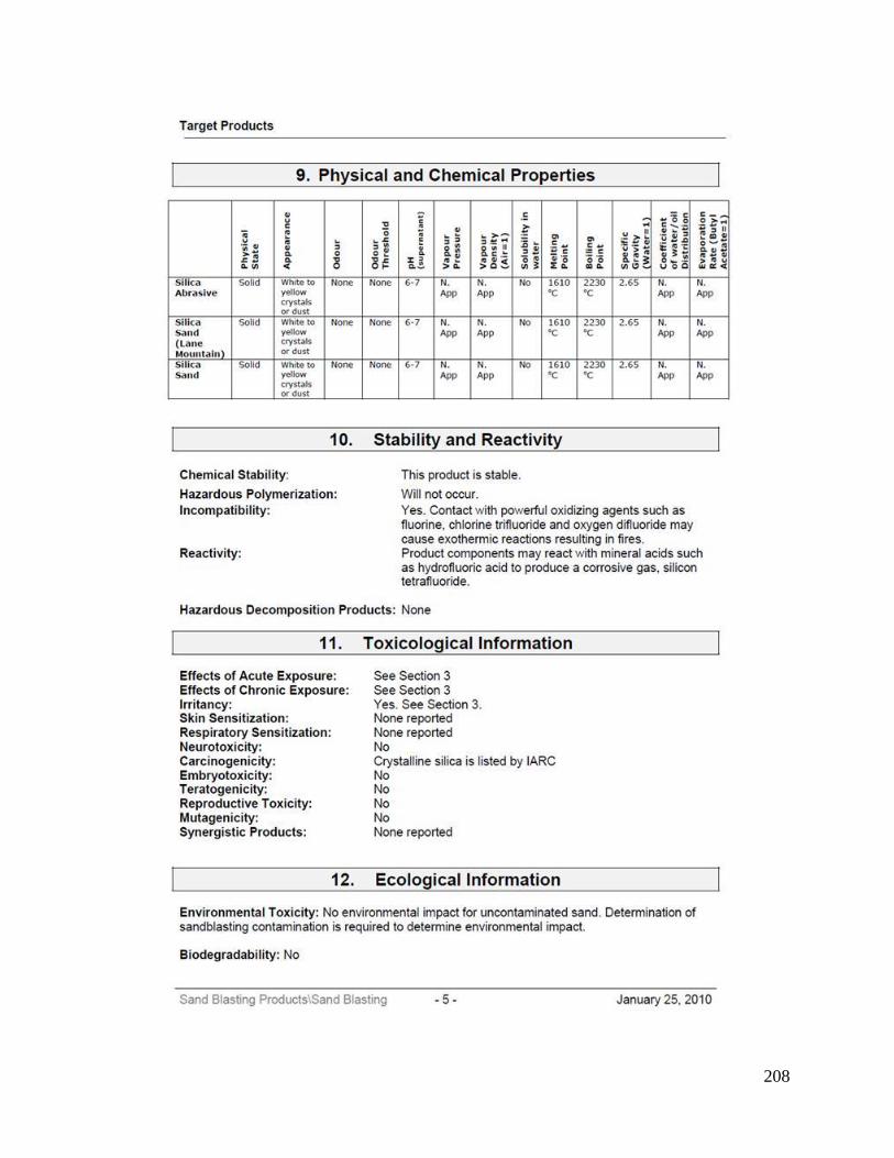
208

209

210
A1-3: SAG Discharge, Lead-Zinc Ore Sample

211

212

213
Appendix A2: Assay Analysis
Sample Elements
Pb Zn Fe Al2O3 BaO CaO Cr2O3 Fe2O3 K2O MgO MnO
Silica Sample - - - 0.54 <0.01 0.11 0.05 0.52 0.18 0.03 <0.01
Galena Concentrate 82.7 1.49 0.26 0.07 - 0.03 <0.01 0.36 0.02 0.01 <0.01
Lead Zinc Ore 9.30 19.8 7.00 0.83 - 0.87 0.02 10.35 0.11 0.08 0.02
Na2O P2O5 SiO2 TiO2
Silica Sample 0.19 0.05 92.1 0.06
Galena Concentrate 0.17 - 0.34 <0.01
Lead Zinc Ore 0.10 - 31.7 0.02
% % % % % % % % % % %
Analytical Laboratory Manager
ISO 9001:2008Certificate No. FS63170
Date: April 15th, 2011
University of British Columbia - KM3009
Certificate of Analysis

214
Appendix A3: Measured Specific Gravity, SG

215
Appendix A4: Experimental Data
Table A4-1: Quartz Experimental Data at 1000 rpm
ISA-Mill Grind Tests Data Sheet
Feed material type: Quartz Galena Ore Mix Date: Jan 29, '10
SG 2.629 7.19 3.662 3.296 Test No: Q1000
Target RPM 1000
Set Flow rate (L/min): ~ 3.5
Starting Flow Rate: 77.10% 860 mL 15.03 sec ===> 3.433 L/min
Pass Number Start RPM
Cummlative
Test Time
(min)
Test Time
(min)
Residence
Time/4L mill
volume (min)
Temp (oC)
Pressure
(bar)
Power
(KW)
Flow Rate
(L/min)
Cummulative Energy
(KWhr)
Energy Read
(KWhr)
Calculated
Energy
(KWhr)
Net
Calculate
d Power
(KW)
1 1000 6.82 6.82 1.04 21 0.4 0.7 3.43 92.09 0.11 0.023 0.2
2 1000 13.35 6.53 2.03 22 0.35 0.7 3.52 92.19 0.10 0.022 0.2
3 1000 19.88 6.53 3.02 22.5 0.4 0.7 3.51 92.29 0.10 0.022 0.2
4 1000 26.30 6.42 4.00 24 0.4 0.7 3.44 92.38 0.09 0.021 0.2
5 1000 32.68 6.38 4.97 25 0.4 0.7 3.34 92.47 0.09 0.021 0.2
Silica: 30.8% solids wt Solid Mass 10kg + Liquid 22.5L Galena: 54.5% solids wt Solid Mass 10kg + Liquid 8.3L Initial Energy @ T0 = 91.98 KWhr
14.29% solids vol Solid Mass 15kg+Liquid 33.7L 14.29% solids vol Solid Mass 15kg+Liquid 12.5L
Solid Mass 5kg+Liquid 11.2L Solid Mass 5kg+Liquid 4.17L
Discarded first 40 seconds of the first Run. Flush mill with water until water comes out clear beore second Test. Non-stop between passes, consistent flow pattern in the mill. First 30 seconds are in the feed tank,
since what is left in the mill is from previous pass.

216
Table A4-2: Quartz Experimental Data at 1500 rpm
ISA-Mill Grind Tests Data Sheet
Feed material type: Quartz Galena Ore Mix Date: Jan 29, '10
SG 2.629 7.19 3.662 3.296 Test No: Q1500
Target RPM 1500
Set Flow rate (L/min): ~ 3.5 max
Starting Flow Rate: 77.10% 870 mL 15.06 sec ===> 3.466 L/min
Pass Number Start RPMCummlative
Test TimeTest Time
Residence
Time/4L mill
volume (min)
Temp (oC)
Pressure
(bar)
Power
(KW)
Flow Rate
(L/min)
Cummulative Energy
(KWhr)
Energy Read
(KWhr)
Calculated
Energy
(KWhr)
Net
Calculated
Power
(KW)
1 1490 6.97 6.97 1.06 19.00 0.45 1.6 3.43 92.94 0.22 0.093 0.8
2 1490 13.87 6.90 2.11 22.50 0.45 1.7 3.45 93.15 0.21 0.104 0.9
3 1490 20.55 6.68 3.13 26.00 0.45 1.7 3.39 93.36 0.21 0.100 0.9
4 1490 27.02 6.47 4.11 28.00 0.45 1.6 3.41 93.55 0.19 0.086 0.8
5 1490 33.52 6.50 5.10 30.00 0.45 1.5 3.44 93.74 0.18 0.076 0.7
Silica: 30.8% solids wt Solid Mass 10kg + Liquid 22.5L Galena: 54.5% solids wt Solid Mass 10kg + Liquid 8.3L Initial Energy @ T0 = 92.71 KWhr
14.29% solids vol Solid Mass 15kg+Liquid 33.7L 14.29% solids vol Solid Mass 15kg+Liquid 12.5L
Solid Mass 5kg+Liquid 11.2L Solid Mass 5kg+Liquid 4.17L
Discarded first 40 seconds of the first Run. Flush mill with water until water comes out clear beore second Test. Non-stop between passes, consistent flow pattern in the mill. First 30 seconds are in the feed tank,
since what is left in the mill is from previous pass.

217
Table A4-3: Quartz Experimental Data at 2000 rpm
ISA-Mill Grind Tests Data Sheet
Feed material type: Quartz Galena Ore Mix Date: Jan 29, '10
SG 2.629 7.19 3.662 3.296 Test No: Q2000
Target RPM 2000
Set Flow rate (L/min): ~ 3.5 max
Starting Flow Rate: 77.00% 965 mL 16.94 sec ===> 3.418 L/min
Pass Number start RPMCummlative
Test TimeTest Time
Residence
Time/4L mill
volume (min)
Temp (oC)
Pressure
(bar)
Power
(KW)
Flow Rate
(L/min)
Cummulative Energy
(KWhr)
Energy Read
(KWhr)
Calculated
Energy
(KWhr)
Net
Calculated
Power
(KW)
1 1940 6.92 6.92 1.05 23.00 0.50 2.7 3.46 95.42 0.34 0.18 1.6
2 1950 13.17 6.25 2.00 29.00 0.50 2.5 3.51 95.70 0.28 0.15 1.4
3 1950 19.42 6.25 2.95 31.00 0.55 2.5 3.37 95.98 0.28 0.15 1.4
4 1950 25.58 6.17 3.89 35.00 0.55 2.5 3.40 96.25 0.27 0.14 1.4
5 1950 32.10 6.52 4.88 37.00 0.55 2.5 3.52 96.55 0.30 0.15 1.4
Silica: 30.8% solids wt Solid Mass 10kg + Liquid 22.5L Galena: 54.5% solids wt Solid Mass 10kg + Liquid 8.3L Initial Energy @ T0 = 95.08 KWhr
14.29% solids vol Solid Mass 15kg+Liquid 33.7L 14.29% solids vol Solid Mass 15kg+Liquid 12.5L
Solid Mass 5kg+Liquid 11.2L Solid Mass 5kg+Liquid 4.17L
Discarded first 40 seconds of the first Run. Flush mill with water until water comes out clear beore second Test. Non-stop between passes, consistent flow pattern in the mill. First 30 seconds are in the feed tank,
since what is left in the mill is from previous pass.

218
Table A4-4: Galena Concentrate Experimental Data at 1000 rpm
ISA-Mill Grind Tests Data Sheet
Feed material type: Quartz Galena Ore Mix Date: Jan 30, '10
SG 2.629 7.19 3.662 3.296 Test No: G1000
Target RPM 1000
Set Flow rate (L/min): ~ 3.5 max
Starting Flow Rate: 77.00% 870 mL 14.81 sec ===> 3.525 L/min
Pass Number start RPMCummlative
Test TimeTest Time
Residence
Time/4L mill
volume (min)
Temp (oC)
Pressure
(bar)
Power
(KW)
Flow Rate
(L/min)
Cummulative Energy
(KWhr)
Energy Read
(KWhr)
Calculated
Power
(KWhr)
Net
Calculated
Power
(KW)
1 1000 3.30 3.30 0.90 23.00 0.4 0.8 3.51 98.30 0.06 0.02 0.3
2 1000 6.73 3.43 1.85 23.50 0.4 0.8 3.53 98.36 0.05 0.02 0.3
3 1000 9.73 3.00 2.67 24.00 0.4 0.8 3.35 98.40 0.05 0.02 0.3
4 1000 12.68 2.95 3.48 24.00 0.5 0.7 3.52 98.44 0.04 0.01 0.2
5 1000 15.55 2.87 4.26 24.50 0.5 0.7 3.39 98.49 0.04 0.01 0.2
Silica: 30.8% solids wt Solid Mass 10kg + Liquid 22.5L Galena: 54.5% solids wt Solid Mass 10kg + Liquid 8.3L Initial Energy @ T0 = 98.24 KWhr
14.29% solids vol Solid Mass 15kg+Liquid 33.7L 14.29% solids vol Solid Mass 15kg+Liquid 12.5L
Solid Mass 5kg+Liquid 11.2L Solid Mass 5kg+Liquid 4.17L
Discarded first 40 seconds of the first Run. Flush mill with water until water comes out clear beore second Test. Non-stop between passes, consistent flow pattern in the mill. First 30 seconds are in the feed tank, since what is left
in the mill is from previous pass.

219
Table A4-5: Galena Concentrate Experimental Data 1500 rpm
ISA-Mill Grind Tests Data Sheet
Feed material type: Quartz Galena Ore Mix Date: Jan 30, '10
SG 2.629 7.19 3.662 3.296 Test No: G1500
Target RPM 1500
Set Flow rate (L/min): ~ 3.5 max
Starting Flow Rate: 77.00% 870 mL 14.69 sec ===> 3.553 L/min
Pass Number start RPMCummlative
Test TimeTest Time
Residence
Time/4L mill
volume (min)
Temp (oC)
Pressure
(bar)
Power
(KW)
Flow Rate
(L/min)
Cummulative Energy
(KWhr)
Energy Read
(KWhr)
Calculated
Power
(KWhr)
Net
Calculated
Power
(KW)
1 1500 3.87 3.87 1.06 21.00 0.70 1.9 3.50 99.61 0.13 0.07 1.10
2 1500 7.73 3.87 2.12 23.00 0.80 1.55 3.46 99.72 0.11 0.05 0.75
3 1500 11.50 3.77 3.15 25.50 0.80 1.8 3.48 99.84 0.12 0.06 1.00
4 1500 15.35 3.85 4.21 27.00 0.60 1.6 3.63 99.95 0.12 0.05 0.80
5 1500 18.87 3.52 5.17 30.00 0.70 1.6 3.44 100.06 0.11 0.05 0.80
Silica: 30.8% solids wt Solid Mass 10kg + Liquid 22.5L Galena: 54.5% solids wt Solid Mass 10kg + Liquid 8.3L Initial Energy @ T0 = 99.48 KWhr
14.29% solids vol Solid Mass 15kg+Liquid 33.7L 14.29% solids vol Solid Mass 15kg+Liquid 12.5L
Solid Mass 5kg+Liquid 11.2L Solid Mass 5kg+Liquid 4.17L
Discarded first 40 seconds of the first Run. Flush mill with water until water comes out clear beore second Test. Non-stop between passes, consistent flow pattern in the mill. First 30 seconds are in the feed tank,
since what is left in the mill is from previous pass.

220
Table A4-6: Galena Concentrate Experimental Data at 2000 rpm
ISA-Mill Grind Tests Data Sheet
Feed material type: Quartz Galena Ore Mix Date: Jan 30, '10
SG 2.629 7.19 3.662 3.296 Test No: G2000
Target RPM 2000
Set Flow rate (L/min): ~ 3.5 max
Starting Flow Rate: 77.00% 880 mL 15.09 sec ===> 3.499 L/min
Pass Number start RPMCumulative
Test TimeTest Time
Residence
Time/4L mill
volume (min)
Temp (oC)
Pressure
(bar)
Power
(KW)
Flow Rate
(L/min)
Cumulative Energy
(KWhr)
Energy Read
(KWhr)
Calculated
Power
(KWhr)
Net
Calculated
Power
(KW)
1 2070 * 3.88 3.88 1.06 22.00 1.4/2.3 3.50 3.58 101.09 0.22 0.16 2.40
2 1980 7.48 3.60 2.05 31.00 1.30 3.20 3.46 101.30 0.21 0.13 2.10
3 1980 10.93 3.45 3.00 34.00 1.10 3.10 -- 101.49 0.19 0.12 2.00
4 1980 14.52 3.58 3.98 38.00 1.10 3.10 -- 101.68 0.20 0.12 2.00
5 1980 17.73 3.22 4.86 42.00 1.00 3.10 3.47 101.87 0.18 0.11 2.00
* The pressure during pass1 was approaching the threshold of the machine (2.6 bar), accordingly the rpm was reduced from 2070 to 1980 to avoid tripping off the machine.
Silica: 30.8% solids wt Solid Mass 10kg + Liquid 22.5L Galena: 54.5% solids wt Solid Mass 10kg + Liquid 8.3L Initial Energy @ T0 = 100.872 KWhr
14.29% solids vol Solid Mass 15kg+Liquid 33.7L 14.29% solids vol Solid Mass 15kg+Liquid 12.5L
Solid Mass 5kg+Liquid 4.17L
Discarded first 40 seconds of the first Run. Flush mill with water until water comes out clear before second Test. Non-stop between passes, consistent flow pattern in the mill. First 30 seconds are in the feed tank,
since what is left in the mill is from previous pass.

221
Table A4-7: Mix Quartz and Galena Concentrate Experimental Data at 1000 rpm
ISA-Mill Grind Tests Data Sheet
Feed material type: Quartz Galena Ore Mix Date: April 5, 2010
SG 2.629 7.19 3.662 3.296 Test No: M1000
Target RPM 1000
Set Flow rate (L/min): ~ 3.5 max
Starting Flow Rate: 77.10% 910 mL 15.28 sec ===> 3.573 L/min
Pass Number start RPMCummlative
Test TimeTest Time
Residence
Time/4L mill
volume (min)
Temp (oC)
Pressure
(bar)
Power
(KW)
Flow Rate
(L/min)
Cummulative Energy
(KWhr)
Energy Read
(KWhr)
Calculated
Power
(KWhr)
Net
Calculated
Power
(KW)
1 1000 6.97 6.97 1.09 16.00 0.40 0.80 3.49 141.08 0.11 0.03 0.30
2 1000 13.17 6.20 2.06 18.00 0.35 0.70 3.35 141.16 0.09 0.02 0.20
3 1000 18.73 5.57 2.93 19.00 0.40 0.70 April, 05, '10 141.24 0.08 0.02 0.20
4 1000 24.20 5.47 3.79 20.00 0.40 0.70 3.55 141.32 0.08 0.02 0.20
5 1000 29.55 5.35 4.63 20.00 0.40 0.70 3.57 141.40 0.08 0.02 0.20
Mix: 36% solids wt Solid Mass 12.5kg + Liquid 22.5L Initial Energy @ T0 = 140.96 KWhr
14.29% solids vol
Discarded first 40 seconds of the first Run. Flush mill with water until water comes out clear beore second Test. Non-stop between passes, consistent flow pattern in the mill. First 30 seconds are in the feed tank, since
what is left in the mill is from previous pass.

222
Table A4-8: Mix Quartz and Galena Concentrate Experimental Data at 2000 rpm
ISA-Mill Grind Tests Data Sheet
Feed material type: Quartz Galena Ore Mix Date: April 5, 2010
SG 2.629 7.19 3.662 3.296 Test No: M2000
Target RPM 2000
Set Flow rate (L/min): ~ 3.5 max
Starting Flow Rate: 77.30% 900 mL 15.14 sec ===> 3.567 L/min
Pass Number start RPMCummlative
Test TimeTest Time
Residence
Time/4L mill
volume (min)
Temp (oC)
Pressure
(bar)
Power
(KW)
Flow Rate
(L/min)
Cummulative Energy
(KWhr)
Energy Read
(KWhr)
Calculated
Power
(KWhr)
Net
Calculated
Power
(KW)
1 1950 7.30 7.30 1.11 21.00 0.70 3.00 3.57 142.62 0.40 0.23 1.90
2 1950 13.87 6.57 2.11 22.00 0.70 3.00 3.51 142.96 0.34 0.21 1.90
3 1950 20.30 6.43 3.09 22.50 0.70 2.70 3.43 143.28 0.31 0.17 1.60
4 1950 27.47 7.17 4.18 24.00 0.70 2.70 3.61 143.61 0.34 0.19 1.60
5 1950 33.43 5.97 5.08 25.00 0.70 2.60 3.51 143.89 0.28 0.15 1.50
Mix: 36% solids wt Solid Mass 12.5kg + Liquid 22.5L Initial Energy @ T0 = 142.22 KWhr
14.29% solids vol
Discarded first 40 seconds of the first Run. Flush mill with water until water comes out clear beore second Test. Non-stop between passes, consistent flow pattern in the mill. First 30 seconds are in the feed tank,
since what is left in the mill is from previous pass.

223
Table A4-9: Lead-Zinc Ore Experimental Data at 1000 rpm
ISA-Mill Grind Tests Data Sheet
Feed material type: Quartz Galena Ore Mix Date: April 5, 2010
SG 2.629 7.19 3.662 3.296 Test No: O1000
Target RPM 1000
Set Flow rate (L/min): ~ 3.5 max
Starting Flow Rate: 78.00% 900 mL 15.54 sec ===> 3.475 L/min
Pass Number start RPMCummlative
Test TimeTest Time
Residence
Time/4L mill
volume (min)
Temp (oC)
Pressure
(bar)
Power
(KW)
Flow Rate
(L/min)
Cummulative Energy
(KWhr)
Energy Read
(KWhr)
Calculated
Power
(KWhr)
Net
Calculated
Power
(KW)
1 980 4.38 4.38 0.67 16.00 0.40 0.70 3.55 144.06 0.07 0.01 0.20
2 980 8.87 4.48 1.35 17.00 0.40 0.70 --- 144.12 0.07 0.01 0.20
3 980 12.95 4.08 1.97 19.00 0.40 0.70 3.43 144.18 0.06 0.01 0.20
4 980 16.98 4.03 2.58 20.00 0.40 0.70 --- 144.24 0.06 0.01 0.20
5 980 20.68 3.70 3.15 21.00 0.40 0.70 3.56 144.30 0.05 0.01 0.20
Mix: 36% solids wt Solid Mass 12.5kg + Liquid 22.5L Initial Energy @ T0 = 143.99 KWhr
14.29% solids vol
Discarded first 40 seconds of the first Run. Flush mill with water until water comes out clear beore second Test. Non-stop between passes, consistent flow pattern in the mill. First 30 seconds are in the feed tank,
since what is left in the mill is from previous pass.

224
Table A4-10: Lead-Zinc Ore Experimental Data at 1500 rpm
ISA-Mill Grind Tests Data Sheet
Feed material type: Quartz Galena Ore Mix Date: April 5, 2010
SG 2.629 7.19 3.662 3.296 Test No: O1500
Target RPM 1500
Set Flow rate (L/min): ~ 3.5 max
Starting Flow Rate: 78.00% 840 mL 15.47 sec ===> 3.468 L/min
Pass Number start RPMCummlative
Test TimeTest Time
Residence
Time/4L mill
volume (min)
Temp (oC)
Pressure
(bar)
Power
(KW)
Flow Rate
(L/min)
Cummulative Energy
(KWhr)
Energy Read
(kWhr)
Calculated
Energy
(KWhr)
Net
Calculated
Power
(KW)
1 1500 5.32 5.32 0.81 18.00 0.50 1.60 3.49 144.77 0.16 0.07 0.80
2 1510 11.00 5.68 1.67 18.00 0.50 1.60 --- 144.94 0.17 0.08 0.80
3 1510 15.73 4.73 2.39 24.00 0.50 1.50 3.58 145.07 0.14 0.06 0.70
4 1510 20.88 5.15 3.18 26.00 0.50 1.50 --- 145.22 0.14 0.06 0.70
5 1510 25.40 4.52 3.86 27.00 0.50 1.50 3.24 145.34 0.13 0.05 0.70
Mix: 36% solids wt Solid Mass 12.5kg + Liquid 22.5L Initial Energy @ T0 = 144.61 KWhr
14.29% solids vol
Discarded first 40 seconds of the first Run. Flush mill with water until water comes out clear beore second Test. Non-stop between passes, consistent flow pattern in the mill. First 30 seconds are in the feed tank,
since what is left in the mill is from previous pass.

225
Table A4-11: Lead-Zinc Ore Experimental Data at 2000 rpm
ISA-Mill Grind Tests Data Sheet
Feed material type: Quartz Galena Ore Mix Date: April 5, 2010
SG 2.629 7.19 3.662 3.296 Test No: O2000
Target RPM 2000
Set Flow rate (L/min): ~ 3.5 max
Starting Flow Rate: 77.20% 920 mL 15.59 sec ===> 3.541 L/min
Pass Number start RPMCummlative
Test TimeTest Time
Residence
Time/4L mill
volume (min)
Temp (oC)
Pressure
(bar)
Power
(KW)
Flow Rate
(L/min)
Cummulative Energy
(KWhr)
Energy Read
(KWhr)
Calculated
Energy
(KWhr)
Net
Calculated
Power
(KW)
1 1980 5.08 5.08 0.77 23.00 0.60 3.00 3.67 146.09 0.27 0.16 1.90
2 1980 10.38 5.30 1.58 26.00 0.70 2.80 --- 146.35 0.27 0.15 1.70
3 1990 15.22 4.83 2.31 31.00 0.70 2.70 --- 146.59 0.23 0.13 1.60
4 1990 20.05 4.83 3.05 33.00 0.70 2.70 --- 146.92 0.33 0.13 1.60
5 1990 26.42 6.37 4.02 41.00 0.70 2.70 3.50 147.12 0.21 0.17 1.60
Mix: 36% solids wt Solid Mass 12.5kg + Liquid 22.5L Initial Energy @ T0 = 145.82 KWhr
14.29% solids vol
Discarded first 40 seconds of the first Run. Flush mill with water until water comes out clear beore second Test. Non-stop between passes, consistent flow pattern in the mill. First 30 seconds are in the feed tank,
since what is left in the mill is from previous pass.

226
Appendix A5: Cyclone Correlation Factor
Table A5: Cyclone Correlation Factor for Quartz, Galena Concentra, Mixed Quartz and Galena, Lead-Zinc Ore Samples
Material
Temp (oC) Flow Rate (mm/min) Elutriation Time (min) SG
Total
Correction
Factor Measure
Correction
Factor Measure
Correction
Factor Measure
Correction
Factor Measure
Correction
Factor
Quartz 5.3 1.225 181 0.992 20 0.995 2.629 1.00 1.161
Galena
Concentrate 5.2 1.225 180 0.992 20 0.995 7.19 0.51 0.592
Mixed Quartz
and Galena 7.7 1.180 180 0.992 20 0.955 3.296 0.85 0.950
Lead-Zinc Ore 7.8 1.180 180 0.992 20 0.995 3.662 0.77 0.861

227
Appendix B: Experimental Results
Appendix B1: Mass of Solids Calculations Based on Volume Percent
Target % Solids by Volume = 14.29 %
SG = gm/cm3
(kg/L)
SG-Galena = 7.19 kg/L
SG-Silica = 2.63 kg/L
SG-Ore = 3.662 kg/L
SG-Mix = 3.296 kg/L
Mass Solids Galena = 27.0 kg ====> % Solids by weight : 54.5 for 15 kg solids => 12.5 Liter of water
Mass Solids Silica = 9.9 kg 30.5 for 10 kg solids => 22.5 Liter of water
MassSolids Ore = 13.7 kg 37.9 for 10 kg solids => 16.4 Liter of water
Mass Solid Mix = 12.4 kg 35.5 for 10 kg solids => 18.2 Liter of water

228
Appendix B2: Rosin Rammler Fit and Parameters
Table B2-1: Rosin Rammler Parameters for Quartz at 1000 rpm
Figure B2-1: Rosin Rammler Fit superimposed on PSD for Quartz at 1000 rpm
Quartz - 1000 RPM
Pass Slope (b) (a) P80 R2
Feed 4.42 74.52 97.38 0.98
Q1000-P1 2.26 78.28 90.57 0.94
Q1000-P2 2.20 73.12 87.68 0.94
Q1000-P3 2.13 68.09 86.12 0.94
Q1000-P4 2.08 62.94 78.72 0.95
Q1000-P5 2.05 56.79 74.95 0.93
0
10
20
30
40
50
60
70
80
90
100
0.1 1 10 100 1000
% P
ass
ing
Size (m)
Quartz - 1000 RPM - Pass
Feed
RR-Feed
Q1000-P1
RR-P1
Q1000-P2
RR-P2
Q1000-P3
RR-P3
Q1000-P4
RR-P4
Q1000-P5
RR-P5

229
Table B2-2: Rosin Rammler Parameters for Quartz at 1500 rpm
Figure B2-2: Rosin Rammler Fit superimposed on PSD for Quartz at 1500 rpm
Quartz - 1500 RPM
Pass Slope (b) (a) P80 R2
Q1500-P1 2.06 58.89 80.10 0.93
Q1500-P2 1.86 46.21 67.81 0.95
Q1500-P3 1.82 38.21 55.94 0.95
Q1500-P4 1.80 30.35 40.39 0.93
Q1500-P5 1.67 28.15 34.71 0.93
0
10
20
30
40
50
60
70
80
90
100
0.1 1 10 100 1000
% P
ass
ing
Size (m)
Quartz - 1500 RPM - Pass
Feed
RR-Feed
Q1500-P1
RR-P1
Q1500-P2
RR-P2
Q1500-P3
RR-P3
Q1500-P4
RR-P4
Q1500-P5
RR-P5

230
Table B2-3: Rosin Rammler Parameters for Quartz at 2000 rpm
Figure B2-3: Rosin Rammler Fit superimposed on PSD for Quartz at 2000 rpm
Quartz - 2000 RPM
Pass Slope (b) (a) P80 R2
Q2000-P1 1.86 46.66 67.66 0.96
Q2000-P2 1.81 33.36 43.41 0.94
Q2000-P3 1.69 28.09 32.39 0.93
Q2000-P4 1.66 23.56 24.18 0.91
Q2000-P5 1.65 19.80 20.04 0.91
0
10
20
30
40
50
60
70
80
90
100
0.1 1 10 100 1000
% P
ass
ing
Size (m)
Quartz - 2000 RPM - Pass
Feed
RR-Feed
Q2000-P1
RR-P1
Q2000-P2
RR-P2
Q2000-P3
RR-P3
Q2000-P4
RR-P4
Q2000-P5
RR-P5

231
Table B2-4: Rosin Rammler Parameters for Galena at 1000 rpm
Figure B2-4: Rosin Rammler Fit superimposed on PSD for Galena at 1000 rpm
Galena - 1000 RPM
Pass Slope (b) (a) P80 R2
Feed 1.34 60 96.6 0.96
G1000-P1 2.01 32 47.7 0.92
G1000-P2 1.69 33 33.8 0.92
G1000-P3 2.07 28 25.3 0.90
G1000-P4-2 2.08 21 21.1 0.91
G1000-P5-2 1.53 22 21.3 0.96
0
10
20
30
40
50
60
70
80
90
100
1 10 100 1000
% P
ass
ing
size (m)
Galena - 1000 RPM
Feed
RR-Feed
G1000-P1
RR-P1
G1000-P2
RR-P2
G1000-P3
RR-P3
G1000-P4-2
RR-P4
G1000-P5-2
RR-P5

232
Table B2-5: Rosin Rammler Parameters for Galena at 1500 rpm
Figure B2-5: Rosin Rammler Fit superimposed on PSD for Galena at 1500 rpm
Galena - 1500 RPM
Pass Slope (b) (a) P80 R2
G1500-P1 2.02 22 23.4 0.89
G1500-P2 1.95 22 18.7 0.89
G1500-P3 1.99 21 17.2 0.89
G1500-P4 1.84 18 13.1 0.85
G1500-P5 1.75 16 11.9 0.82
0
10
20
30
40
50
60
70
80
90
100
1 10 100 1000
% P
ass
ing
size (m)
Galena - 1500 RPM
Feed
RR-Feed
G1500-P1
RR-P1
G1500-P2
RR-P2
G1500-P3
RR-P3
G1500-P4-2
RR-P4
G1500-P5-2
RR-P5

233
Table B2-6: Rosin Rammler Parameters for Galena at 2000 rpm
Figure B2-6: Rosin Rammler Fit superimposed on PSD for Galena at 2000 rpm
Galena - 2000 RPM
Pass Slope (b) (a) P80 R2
G2000-P1 1.62 20 14.0 0.82
G2000-P2 1.69 17 13.2 0.89
G2000-P3-2 1.30 23 13.2 0.84
G2000-P4 1.20 18 12.7 0.84
G2000-P5 1.05 18 12.8 0.84
0
10
20
30
40
50
60
70
80
90
100
1 10 100 1000
% P
ass
ing
size (m)
Galena - 2000 RPM Feed
RR-Feed
G2000-P1
RR-P1
G2000-P2
RR-P2
G2000-P3
RR-P3
G2000-P4
RR-P4
G2000-P5
RR-P5

234
Table B2-7: Rosin Rammler Parameters for Mixed quartz and galena Sample at 1000 rpm
Figure B2-7: Rosin Rammler Fit superimposed on PSD
for Mixed quartz and galena Sample at 1000 rpm
Mix - 1000
Pass Slope (b) (a) P80 R2
Feed 1.46 109.1 122.8 0.92
M1000-P1 1.47 109.5 119.9 0.95
M1000-P2 1.36 110.8 119.4 0.95
M1000-P3 1.32 88.39 109.8 0.97
M1000-P5 1.30 80.09 105.8 0.97
M1000-P4-2 1.35 72.66 100.9 0.96
0
10
20
30
40
50
60
70
80
90
100
1 10 100 1000
% P
ass
ing
size (m)
Mix - 1000 RPM
Feed
RR-Feed
M1000-P1
RR-P1
M1000-P2
RR-P2
M1000-P3
RR-P3
M1000-P4
RR-P4
M1000-P5
RR-P5

235
Table B2-8: Rosin Rammler Parameters for Mixed quartz and galena Sample at 2000 rpm
Figure B2-8: Rosin Rammler Parameters
for Mixed quartz and galena Sample at 2000 rpm
Mix - 2000
Pass Slope (b) (a) P80 R2
M2000-P1 1.22 53.93 82.7 0.98
M2000-P2 1.19 29.94 47.3 0.99
M2000-P3 0.98 27.11 33.9 0.95
M2000-P4 0.85 20.66 22.5 0.89
M2000-P5 1.00 14.99 17.2 0.94
0
10
20
30
40
50
60
70
80
90
100
1 10 100 1000
% P
ass
ing
size (m)
Mix - 2000 RPM
Feed
RR-Feed
M2000-P1
RR-P1
M2000-P2
RR-P2
M2000-P3
RR-P3
M2000-P4
RR-P4
M2000-P5
RR-P5

236
Table B2-9: Rosin Rammler Parameters for Lead-Zinc Ore at 1000 rpm
Figure B2-9: Rosin Rammler Parameters for Lead-Zinc Ore at 1000 rpm
Ore - 1000
Pass Slope (b) a P80 R2
Feed 1.12 59.52 96.2 0.97
O1000-P1 1.20 37.40 63.0 0.97
O1000-P2 1.20 34.30 56.2 0.97
O1000-P3 1.23 33.99 54.1 0.98
O1000-P4 1.20 29.75 44.5 0.98
O1000-P5 1.24 25.44 35.9 0.98
0
10
20
30
40
50
60
70
80
90
100
1 10 100 1000
% P
ass
ing
size (mm)
Ore - 1000 RPM
Feed
RR-Feed
O1000-P1
RR-P1
O1000-P2
RR-P2
O1000-P3
RR-P3
O1000-P4
RR-P4
O1000-P5
RR-P5

237
Table B2-10: Rosin Rammler Parameters for Lead-Zinc Ore at 1500 rpm
Figure B2-10: Rosin Rammler Parameters for Lead-Zinc Ore at 1500 rpm
Ore - 1500
Pass Slope (b) a P80 R2
O1500-P1 1.23 30.33 46.5 0.98
O1500-P2 1.22 24.92 31.9 0.97
O1500-P3 1.00 24.74 25.9 0.92
O1500-P4 0.89 21.03 20.0 0.86
O1500-P5 1.23 14.97 16.3 0.96
0
10
20
30
40
50
60
70
80
90
100
1 10 100 1000
% P
ass
ing
size (mm)
Ore - 1500 RPM
Feed
RR-Feed
O1500-P1
RR-P1
O1500-P2
RR-P2
O1500-P3
RR-P3
O1500-P4
RR-P4
O1500-P5
RR-P5

238
Table B2-11: Rosin Rammler Parameters for Lead-Zinc Ore at 2000 rpm
Figure B2-11: Rosin Rammler Parameters for Lead-Zinc Ore at 2000 rpm
Ore - 2000
Pass Slope (b) a P80 R2
O2000-P1 1.02 29.39 34.2 0.93
O2000-P2 0.90 21.16 20.0 0.86
O2000-P3 0.90 17.48 16.8 0.85
O2000-P4 0.82 13.90 13.0 0.80
O2000-P5 0.74 13.70 11.7 0.75
0
10
20
30
40
50
60
70
80
90
100
1 10 100 1000
% P
ass
ing
size (mm)
Ore - 2000 RPM
Feed
RR-Feed
O2000-P1
RR-P1
O2000-P2
RR-P2
O2000-P3
RR-P3
O2000-P4
RR-P4
O2000-P5
RR-P5

239
Appendix B3: Correlation between Measured and Calculated P80
(Initial and Post Initial) Data
Figure B3-1: Quartz Correlation; (a) Initial Breakage; (b) Average breakage
60
70
80
90
100
60 70 80 90 100
Ca
lcu
late
d P
80
(
m)
Measured P80 (m)
Quartz - Initial
Exponential 1000
Linear 1000
Exponenial 1500
Linear 1500
Exponential 2000
Linear 2000
10
20
30
40
50
60
70
80
90
100
10 20 30 40 50 60 70 80 90 100
Ca
lcu
late
d P
80
(
m)
Measured P80 (m)
Quartz - Average Berakage (P1-P5)
Exponential 1000
Linear 1000
Exponential 1500
Linear 1500
Exponential 2000
Linear 2000
(a)
(b)

240
Figure B3-2: Galena Concentrate Correlation; (a) Initial Breakage; (b) Average breakage
10
20
30
40
50
60
70
80
90
100
10 20 30 40 50 60 70 80 90 100
Ca
lcu
late
d P
80
(
m)
Measured P80 (m)
Galena Concentrate - Initial
Exponential 1000
Linear 1000
Exponential 1500
Linear1500
Exponential 2000
Linear2000
10
15
20
25
30
35
40
45
50
10 20 30 40 50
Ca
clc
ula
ted
P8
0 (
m)
Measured P80 (m)
Galena Concentrate
Average Berakage (P1-P5)
Exponential 1000
Linear 1000
Exponential 1500
Linear 1500
Exponential 2000
Linear 2000
(a)
(b)

241
Figure B3-3: Mixed Quartz and Galena Correlation;
(a) Initial Breakage; (b) Average Breakage
60
70
80
90
100
110
120
130
60 70 80 90 100 110 120 130
Ca
lcu
late
d P
80
(
m)
Measured P80 (m)
Mixed Sample - Initial
Exponential 1000
Linear 1000
Exponential 2000
Linear 2000
10
30
50
70
90
110
130
10 30 50 70 90 110 130
Ca
lcu
late
d P
80
(
m)
Measured P80 (m)
Mixed Sample
Average Berakage (P1-P5)
Exponential 1000
Linear 1000
Exponential 2000
Linear 2000
(b) (a)
(b)

242
Figure B3-4: Lead-Zinc Ore Correlation; (a) Initial Breakage; (b) Average breakage
30
40
50
60
70
80
90
100
30 40 50 60 70 80 90 100
Ca
lcu
late
d P
80
(
m)
Measured P80 (mm)
Lead-Zinc Ore - Initial
Exponential 1000
Linear 1000
Exponential 1500
Linear 1500
Exponential 2000
Linear 2000
30
35
40
45
50
55
60
65
70
30 35 40 45 50 55 60 65 70
Ca
lcu
late
d P
80
(
m)
Measured P80 (m)
Lead-Zinc Ore Sample
Average Berakage (P1-P5)
Exponential 1000
Linear 1000
Exponential 1500
Linear 1500
Exponential 2000
Linear 2000
(a)
(b)

243
Appendix B4: Energy Breakage vs. Particle Size P80 (m)
Figure B4-1: Net Energy vs. Particle Size for Quartz
Figure B4-2: Net Energy vs. Particle Size for Galena Concentrate
y = 44285e-0.087x
R² = 0.8328
y = 675.09e-0.029x
R² = 0.8681
y = 660.33e-0.029x
R² = 0.9748
0
100
200
300
400
500
1 10 100
Net
En
erg
y (
KJ
)
Particle Size P80 (m)
Quartz Sample
Q1000
Q1500
Q2000
y = 115.99e-0.04x
R² = 0.927
y = 932.29e-0.111x
R² = 0.8726
y = 2E+08e-1.028x
R² = 0.9067
0
100
200
300
400
500
600
700
1 10 100
Net
En
erg
y (
KJ
)
Particle Size P80 (m)
Galena Concentrate Sample
G1000
G1500
G2000

244
Figure B4-3: Net Energy vs. Particle Size for Mixed Quartz and Galena Sample
Figure B4-4: Net Energy vs. Particle Size for Lead-Zinc Ore Sample
y = 9027.2e-0.05x
R² = 0.9695
y = 640.78e-0.02x
R² = 0.9948
0
100
200
300
400
500
1 10 100 1000
Net
En
erg
y (
KJ
)
Particle Size P80 (m)
Mixed Quartz and Galena Sample
M1000
M2000
y = 303.88e-0.053x
R² = 0.8482
y = 345.42e-0.047x
R² = 0.9982
y = 661.48e-0.061x
R² = 0.9419
0
100
200
300
400
500
1 10 100
Net
En
erg
y (
KJ
)
Particle Size P80 (m)
Lead-Zinc Ore Sample
O1000
O1500
O2000

245
Appendix C: Morphology
Appendix C1: Manual Point Counting Sub-Routine
Sub Morphology()
Dim Roughness As Integer
R1 = 0
R2 = 0
R3 = 0
R4 = 0
R5 = 0
Do
Roughness = Application.InputBox("Enter Roughness Per Particle-Between 1 and 5",
"Roughness Value", "")
If Roughness <> False Then
If Roughness = 1 Then
R1 = R1 + 1
ActiveSheet.Range("rough1").Value = R1
ElseIf Roughness = 2 Then
R2 = R2 + 1
ActiveSheet.Range("C3").Value = R2
ElseIf Roughness = 3 Then
R3 = R3 + 1
ActiveSheet.Range("D3").Value = R3
ElseIf Roughness = 4 Then
R4 = R4 + 1
ActiveSheet.Range("E3").Value = R4
ElseIf Roughness = 5 Then
R5 = R5 + 1
ActiveSheet.Range("F3").Value = R5
Else: MsgBox ("Wrong Value")
End If
End If
Loop Until Roughness = False
End Sub

246
Appendix C2: Snap Shot of the Manual Point Counting Screen
Figure C2-1: Screen Snap Shot of Manual Point Counting and Definition

247
Appendix C3: Manual Point Counting Sensitivity Analysis
Table C3-1: Initial Count of 53m Quartz Sample-Feed
Roughness level
Count %
R1 R2 R3 R4 R5 Total
Counter 1 1 3 20 43 34 100
Counter 2 2 8 22 50 20 100
Table C3--2: After Fine Tuning Roughness Definition Count of 53m Quartz Sample-Feed
Roughness level
Count %
R1 R2 R3 R4 R5 Total
Counter 1 2 7 34 41 18 100
Counter 2 2 7 31 41 21 100
Counter 3 1 5 35 37 23 100
Table C3-3: Count of 13m Quartz Sample-Feed
Roughness level
Count %
R1 R2 R3 R4 R5 Total
Counter 1 0 12 20 62 6 100
Counter 2 0 9 26 61 4 100
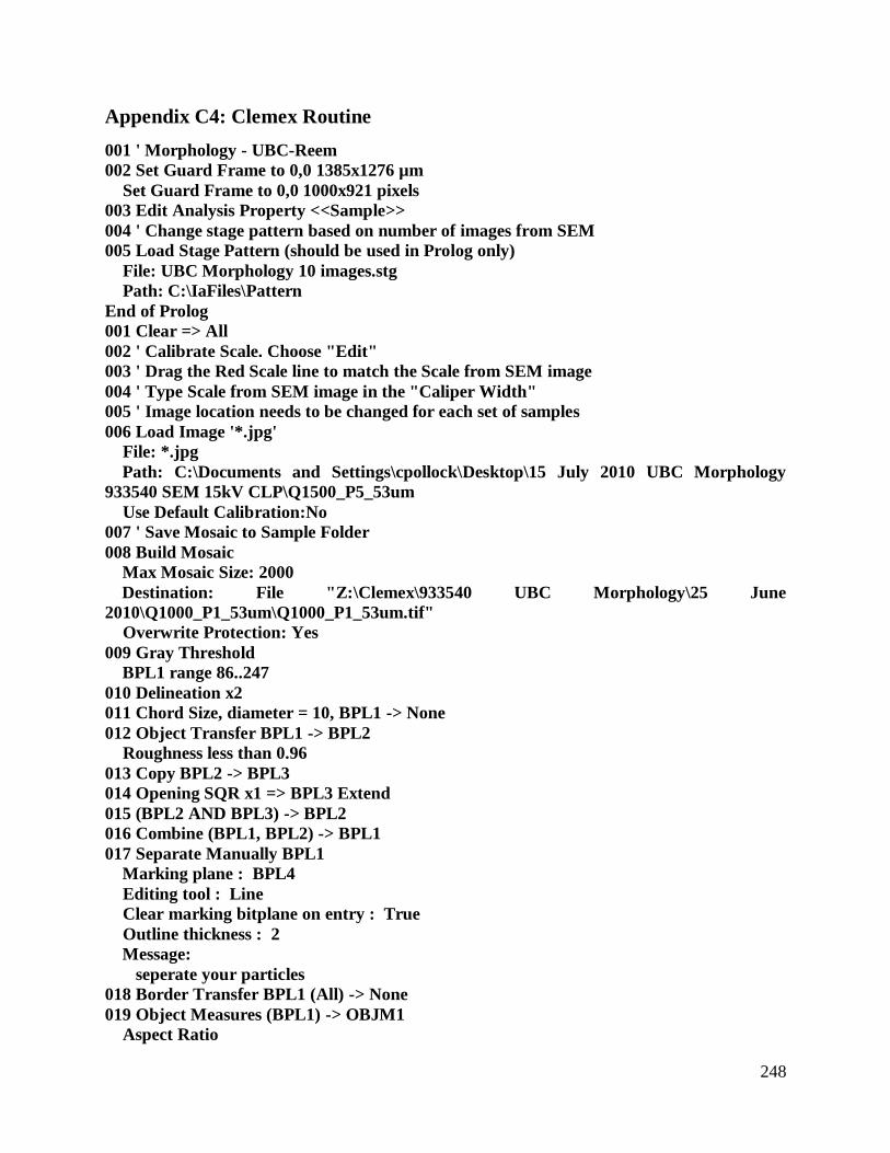
248
Appendix C4: Clemex Routine
001 ' Morphology - UBC-Reem
002 Set Guard Frame to 0,0 1385x1276 µm
Set Guard Frame to 0,0 1000x921 pixels
003 Edit Analysis Property <<Sample>>
004 ' Change stage pattern based on number of images from SEM
005 Load Stage Pattern (should be used in Prolog only)
File: UBC Morphology 10 images.stg
Path: C:\IaFiles\Pattern
End of Prolog
001 Clear => All
002 ' Calibrate Scale. Choose "Edit"
003 ' Drag the Red Scale line to match the Scale from SEM image
004 ' Type Scale from SEM image in the "Caliper Width"
005 ' Image location needs to be changed for each set of samples
006 Load Image '*.jpg'
File: *.jpg
Path: C:\Documents and Settings\cpollock\Desktop\15 July 2010 UBC Morphology
933540 SEM 15kV CLP\Q1500_P5_53um
Use Default Calibration:No
007 ' Save Mosaic to Sample Folder
008 Build Mosaic
Max Mosaic Size: 2000
Destination: File "Z:\Clemex\933540 UBC Morphology\25 June
2010\Q1000_P1_53um\Q1000_P1_53um.tif"
Overwrite Protection: Yes
009 Gray Threshold
BPL1 range 86..247
010 Delineation x2
011 Chord Size, diameter = 10, BPL1 -> None
012 Object Transfer BPL1 -> BPL2
Roughness less than 0.96
013 Copy BPL2 -> BPL3
014 Opening SQR x1 => BPL3 Extend
015 (BPL2 AND BPL3) -> BPL2
016 Combine (BPL1, BPL2) -> BPL1
017 Separate Manually BPL1
Marking plane : BPL4
Editing tool : Line
Clear marking bitplane on entry : True
Outline thickness : 2
Message:
seperate your particles
018 Border Transfer BPL1 (All) -> None
019 Object Measures (BPL1) -> OBJM1
Aspect Ratio

249
Compactness
Roughness
Roundness
Sphericity
Length
Width
Breadth
Perimeter
Convex Perimeter
Area
ASTM E112-96
Angular Position
Volume : Spherical
Volume : Cylindrical
Volume : Ellipsoidal
Volume : Tetragonal
020 ' Change "FldNo" based on number of images from SEM
021 IF FldNo = 20 THEN Next Section
Action: Step out to the Next Section
Display Condition in a Message-Box: No
End of Field
001 ' Save Data to sample folder
002 Export Data OBJM1
File: Q_1500_P5_53um.xls
Path: C:\Documents and Settings\cpollock\Desktop\Q1500
Info Header: Yes
Overwrite Protection: Yes
End of Epilog

250
Appendix C5: Morphology Point Counting Data
Table C5-1A: Morphology Counts for Quartz Sample, Test Run at Agitator Speed 1000 rpm
Particle Counts % Roughness
63 microns Size Fraction 63 microns Size Fraction
Roughness
Level
Residence
Time (min)R1 R2 R3 R4 R5
Total #
of
Particles
Roughness
Level
Residence
Time
(min)
R1 R2 R3 R4 R5
Total #
of
Particles
Qfeed 0.0 13 14 28 162 96 313 Qfeed 0.0 4 4 9 52 31 100
P1 1.0 55 15 41 224 118 453 P1 1.0 12 3 9 49 26 100
P2 2.0 47 14 7 115 73 256 P2 2.0 18 5 3 45 29 100
P3 3.0 42 34 29 132 131 368 P3 3.0 11 9 8 36 36 100
P4 4.0 58 24 32 213 150 477 P4 4.0 12 5 7 45 31 100
P5 5.0 52 30 27 136 102 347 P5 5.0 15 9 8 39 29 100
34 microns Size Fraction 34 microns Size Fraction
Qfeed 0.0 25 32 43 297 91 488 Qfeed 0.0 5 7 9 61 19 100
P1 1.0 13 14 15 119 28 189 P1 1.0 7 7 8 63 15 100
P2 2.0 31 26 23 239 79 398 P2 2.0 8 7 6 60 20 100
P3 3.0 31 15 27 191 68 332 P3 3.0 9 5 8 58 20 100
P4 4.0 45 20 35 237 127 464 P4 4.0 10 4 8 51 27 100
P5 5.0 15 28 38 59 13 153 P5 5.0 10 18 25 39 8 100
15 microns Size Fraction 15 microns Size Fraction
Qfeed 0.0 19 17 14 139 31 220 Qfeed 0.0 9 8 6 63 14 100
P1 1.0 16 19 21 180 45 281 P1 1.0 6 7 7 64 16 100
P2 2.0 12 11 16 167 33 239 P2 2.0 5 5 7 70 14 100
P3 3.0 24 42 30 298 76 470 P3 3.0 5 9 6 63 16 100
P4 4.0 15 19 23 150 46 253 P4 4.0 6 8 9 59 18 100
P5 5.0 6 19 45 114 24 208 P5 5.0 3 9 22 55 12 100

251
Table C5-2A: Morphology Counts for Quartz Sample, Test Run at Agitator Speed 1500 rpm
Particle Counts % Roughness
63 microns Size Fraction 63 microns Size Fraction
Roughness
Level
Residence
Time (min)R1 R2 R3 R4 R5
Total #
of
Particles
Roughness
Level
Residence
Time
(min)
R1 R2 R3 R4 R5
Total #
of
Particles
Qfeed 0.0 13 14 28 162 96 313 Qfeed 0.0 4 4 9 52 31 100
P1 1.1 35 34 64 280 180 593 P1 1.1 6 6 11 47 30 100
P2 2.1 18 27 33 107 41 226 P2 2.1 8 12 15 47 18 100
P3 3.1 25 34 57 209 80 405 P3 3.1 6 8 14 52 20 100
P4 4.1 29 44 61 108 57 299 P4 4.1 10 15 20 36 19 100
P5 5.1 29 32 50 136 31 278 P5 5.1 10 12 18 49 11 100
34 microns Size Fraction 34 microns Size Fraction
Qfeed 0.0 25 32 43 297 91 488 Qfeed 0.0 5 7 9 61 19 100
P1 1.1 17 12 66 305 112 512 P1 1.1 3 2 13 60 22 100
P2 2.1 41 48 94 239 55 477 P2 2.1 9 10 20 50 12 100
P3 3.1 46 62 93 169 21 391 P3 3.1 12 16 24 43 5 100
P4 4.1 48 57 97 141 15 358 P4 4.1 13 16 27 39 4 100
P5 5.1 61 55 63 101 16 296 P5 5.1 21 19 21 34 5 100
15 microns Size Fraction 15 microns Size Fraction
Qfeed 0.0 19 17 14 139 31 220 Qfeed 0.0 9 8 6 63 14 100
P1 1.1 0 6 16 96 10 128 P1 1.1 0 5 13 75 8 100
P2 2.1 3 17 33 156 17 226 P2 2.1 1 8 15 69 8 100
P3 3.1 4 13 27 181 35 260 P3 3.1 2 5 10 70 13 100
P4 4.1 8 7 21 157 48 241 P4 4.1 4 3 9 65 20 100
P5 5.1 19 21 20 202 40 302 P5 5.1 6 7 7 67 13 100

252
Table C5-3A: Morphology Counts for Quartz Sample, Test Run at Agitator Speed 2000 rpm
Particle Counts % Roughness
63 microns Size Fraction 63 microns Size Fraction
Roughness
Level
Residence
Time (min)R1 R2 R3 R4 R5
Total #
of Particles
Roughness
Level
Residence
Time (min)R1 R2 R3 R4 R5
Total #
of
Particles
Qfeed 0.0 13 14 28 162 96 313 Qfeed 0.0 4 4 9 52 31 100
P1 1.1 29 39 67 97 72 304 P1 1.1 10 13 22 32 24 100
P2 2.0 39 29 47 88 50 253 P2 2.0 15 11 19 35 20 100
P3 3.0 51 39 34 76 32 232 P3 3.0 22 17 15 33 14 100
P4 3.9 46 50 50 111 5 262 P4 3.9 18 19 19 42 2 100
P5 4.9 78 55 47 115 8 303 P5 4.9 26 18 16 38 3 100
34 microns Size Fraction 34 microns Size Fraction
Qfeed 0.0 25 32 43 297 91 488 Qfeed 0.0 5 7 9 61 19 100
P1 1.1 14 34 82 129 52 311 P1 1.1 5 11 26 41 17 100
P2 2.0 39 37 54 145 84 359 P2 2.0 11 10 15 40 23 100
P3 3.0 35 32 39 143 55 304 P3 3.0 12 11 13 47 18 100
P4 3.9 50 50 43 119 43 305 P4 3.9 16 16 14 39 14 100
P5 4.9 21 12 22 75 34 164 P5 4.9 13 7 13 46 21 100
15 microns Size Fraction 15 microns Size Fraction
Qfeed 0.0 19 17 14 139 31 220 Qfeed 0.0 9 8 6 63 14 100
P1 1.1 6 11 50 131 41 239 P1 1.1 3 5 21 55 17 100
P2 2.0 24 27 36 210 93 390 P2 2.0 6 7 9 54 24 100
P3 3.0 22 18 39 150 66 295 P3 3.0 7 6 13 51 22 100
P4 3.9 28 17 26 75 79 225 P4 3.9 12 8 12 33 35 100
P5 4.9 2 10 18 49 42 121 P5 4.9 2 8 15 40 35 100

253
Table C5-1B Morphology Counts for Galena Concentrate Sample, Test Run at Agitator Speed 1000 rpm
Particle Counts % Roughness
63 microns Size Fraction 63 microns Size Fraction
Roughness
Level
Residence
Time (min)R1 R2 R3 R4 R5
Total #
of
Particles
Roughness
Level
Residence
Time
(min)
R1 R2 R3 R4 R5
Total #
of
Particles
Qfeed 0.00 6 5 22 85 55 173 Qfeed 0.00 3 3 13 49 32 100
P1 0.90 29 8 35 127 74 273 P1 0.90 11 3 13 47 27 100
P2 1.85 14 27 35 85 62 223 P2 1.85 6 12 16 38 28 100
P3 2.67 34 29 35 76 32 206 P3 2.67 17 14 17 37 16 100
P4* 3.48 22 19 20 57 36 154 P4* 3.48 14 12 13 37 23 100
P5 4.26 33 29 20 82 37 201 P5 4.26 16 14 10 41 18 100
* Majority is Sphalerite particles - not counted * Majority is Sphalerite particles - not counted
37 microns Size Fraction 37 microns Size Fraction
Qfeed 0.00 25 17 65 207 162 476 Qfeed 0.00 5 4 14 43 34 100
P1 0.90 47 44 66 239 159 555 P1 0.90 8 8 12 43 29 100
P2 1.85 39 47 72 241 120 519 P2 1.85 8 9 14 46 23 100
P3 2.67 56 78 68 239 87 528 P3 2.67 11 15 13 45 16 100
P4 3.48 43 52 64 226 116 501 P4 3.48 9 10 13 45 23 100
P5 4.26 46 44 30 107 44 271 P5 4.26 17 16 11 39 16 100
17 microns Size Fraction 17 microns Size Fraction
Qfeed 0.00 30 16 71 192 181 490 Qfeed 0.00 6 3 14 39 37 100
P1 0.90 24 28 35 119 67 273 P1 0.90 9 10 13 44 25 100
P2 1.85 52 53 61 222 137 525 P2 1.85 10 10 12 42 26 100
P3 2.67 58 77 80 261 114 590 P3 2.67 10 13 14 44 19 100
P4 3.48 38 20 34 112 63 267 P4 3.48 14 7 13 42 24 100
P5 4.26 68 76 69 244 113 570 P5 4.26 12 13 12 43 20 100

254
Table C5-2B: Morphology Counts for Galena Concentrate Sample, Test Run at Agitator Speed 1500 rpm
Particle Counts % Roughness
63 microns Size Fraction 63 microns Size Fraction
Roughness
Level
Residence
Time (min)R1 R2 R3 R4 R5
Total #
of
Particles
Roughness
Level
Residence
Time
(min)
R1 R2 R3 R4 R5
Total #
of
Particles
Qfeed 0.0 6 5 22 85 55 173 Qfeed 0.0 3 3 13 49 32 100
P1 1.1 29 28 33 67 52 209 P1 1.1 14 13 16 32 25 100
P2 2.1 12 16 12 33 24 97 P2 2.1 12 16 12 34 25 100
P3* 3.2 41 9 6 21 7 84 P3* 3.2 49 11 7 25 8 100
P4 4.2 87 22 10 58 27 204 P4 4.2 43 11 5 28 13 100
P5 5.2 All Smashed particles 0 P5 5.2 All Smashed particles 0
* mostly broken pieces
37 microns Size Fraction 37 microns Size Fraction
Qfeed 0 25 17 65 207 162 476 Qfeed 0 5 4 14 43 34 100
P1 1.1 34 25 39 159 97 354 P1 1.1 10 7 11 45 27 100
P2 2.1 54 66 63 252 90 525 P2 2.1 10 13 12 48 17 100
P3 3.2 92 63 68 191 61 475 P3 3.2 19 13 14 40 13 100
P4 4.2 67 64 33 171 89 424 P4 4.2 16 15 8 40 21 100
P5 5.2 181 106 65 308 95 755 P5 5.2 24 14 9 41 13 100
17 microns Size Fraction 17 microns Size Fraction
Qfeed 0 30 16 71 192 181 490 Qfeed 0 6 3 14 39 37 100
P1 1.1 46 38 41 173 114 412 P1 1.1 11 9 10 42 28 100
P2 2.1 47 47 49 213 164 520 P2 2.1 9 9 9 41 32 100
P3 3.2 63 56 40 193 99 451 P3 3.2 14 12 9 43 22 100
P4 4.2 53 39 23 132 77 324 P4 4.2 16 12 7 41 24 100
P5 5.2 30 31 27 94 36 218 P5 5.2 14 14 12 43 17 100

255
Table C5-3B: Morphology Counts for Galena Concentrate Sample, Test Run at Agitator Speed 2000 rpm
Particle Counts % Roughness
63 microns Size Fraction 63 microns Size Fraction
Roughness
Level
Residence
Time (min)R1 R2 R3 R4 R5
Total #
of
Particles
Roughness
Level
Residence
Time
(min)
R1 R2 R3 R4 R5
Total #
of
Particles
Qfeed 0.0 6 5 22 85 55 173 Qfeed 0.0 3 3 13 49 32 100
P1* 1.1 21 13 7 51 10 102 P1* 1.1 21 13 7 50 10 100
P2 2.1 0 0 0 0 0 0 P2 2.1 0 0 0 0 0 0
P3 3.0 0 0 0 0 0 0 P3 3.0 0 0 0 0 0 0
P4 4.0 0 0 0 0 0 0 P4 4.0 0 0 0 0 0 0
P5 4.9 0 0 0 0 0 0 P5 4.9 0 0 0 0 0 0
* mostly broken pieces
37 microns Size Fraction 37 microns Size Fraction
Qfeed 0.0 25 17 65 207 162 476 Qfeed 0.0 5 4 14 43 34 100
P1 1.1 32 33 28 191 79 363 P1 1.1 9 9 8 53 22 100
P2 2.1 56 52 27 161 61 357 P2 2.1 16 15 8 45 17 100
P3 3.0 131 41 30 141 27 370 P3 3.0 35 11 8 38 7 100
P4 4.0 155 50 36 109 36 386 P4 4.0 40 13 9 28 9 100
P5 4.9 95 40 25 85 27 272 P5 4.9 35 15 9 31 10 100
17 microns Size Fraction 17 microns Size Fraction
Qfeed 0.0 30 16 71 192 181 490 Qfeed 0.0 6 3 14 39 37 100
P1 1.1 18 14 26 103 85 246 P1 1.1 7 6 11 42 35 100
P2 2.1 31 37 30 129 74 301 P2 2.1 10 12 10 43 25 100
P3 3.0 24 39 30 112 68 273 P3 3.0 9 14 11 41 25 100
P4 4.0 21 12 18 91 46 188 P4 4.0 11 6 10 48 24 100
P5 4.9 60 60 49 151 62 382 P5 4.9 16 16 13 40 16 100

256
Table C5-1C: Morphology Counts for Mixed quartz and galena Concentrate Sample (Quartz Counts),
Test Run at Agitator Speed 1000 rpm
Particle Counts % Roughness
63 microns Size Fraction 63 microns Size Fraction
Roughness
Level
Residence
Time (min)R1 R2 R3 R4 R5
Total #
of
Particles
Roughness
Level
Residence
Time
(min)
R1 R2 R3 R4 R5
Total #
of
Particles
Qfeed 0 4 29 45 61 15 154 Qfeed 0.00 3 19 29 40 10 100
P1 1.1 1 37 64 87 18 207 P1 1.09 0 18 31 42 9 100
P2 2.1 7 24 28 51 28 138 P2 2.06 5 17 20 37 20 100
P3 2.9 37 63 52 113 265 P3 2.93 14 24 20 43 0 100
P4* 3.8 26 49 60 87 39 261 P4* 3.79 10 19 23 33 15 100
P5 4.6 30 67 45 69 25 236 P5 4.63 13 28 19 29 11 100
* Majority is Sphalerite particles - not counted * Majority is Sphalerite particles - not counted
36 microns Size Fraction 36 microns Size Fraction
Qfeed 0.0 0 2 3 8 3 16 Qfeed 0.00 0 13 19 50 19 100
P1 1.1 3 7 14 32 15 71 P1 1.09 4 10 20 45 21 100
P2 2.1 1 15 10 36 16 78 P2 2.06 1 19 13 46 21 100
P3 2.9 4 13 26 45 14 102 P3 2.93 4 13 25 44 14 100
P4 3.8 11 31 29 52 35 158 P4 3.79 7 20 18 33 22 100
P5 4.6 18 46 24 55 30 173 P5 4.63 10 27 14 32 17 100
18 microns Size Fraction 18 microns Size Fraction
Qfeed 0.0 0 13 17 55 24 109 Qfeed 0.00 0 12 16 50 22 100
P1 1.1 0 3 7 23 11 44 P1 1.09 0 7 16 52 25 100
P2 2.1 0 5 8 22 9 44 P2 2.06 0 11 18 50 20 100
P3 2.9 0 5 9 30 8 52 P3 2.93 0 10 17 58 15 100
P4 3.8 0 3 5 7 4 19 P4 3.79 0 16 26 37 21 100
P5 4.6 5 19 15 49 17 105 P5 4.63 5 18 14 47 16 100
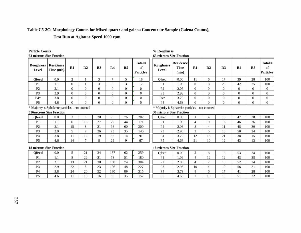
257
Table C5-2C: Morphology Counts for Mixed quartz and galena Concentrate Sample (Galena Counts),
Test Run at Agitator Speed 1000 rpm
Particle Counts % Roughness
63 microns Size Fraction 63 microns Size Fraction
Roughness
Level
Residence
Time (min)R1 R2 R3 R4 R5
Total #
of
Particles
Roughness
Level
Residence
Time
(min)
R1 R2 R3 R4 R5
Total #
of
Particles
Qfeed 0.0 2 1 3 7 5 18 Qfeed 0.00 11 6 17 39 28 100
P1 1.1 0 1 3 5 3 12 P1 1.09 0 8 25 42 25 100
P2 2.1 0 0 0 0 0 0 P2 2.06 0 0 0 0 0 0
P3 2.9 0 0 0 0 0 0 P3 2.93 0 0 0 0 0 0
P4* 3.8 0 0 0 0 0 0 P4* 3.79 0 0 0 0 0 0
P5 4.6 0 0 0 0 0 0 P5 4.63 0 0 0 0 0 0
* Majority is Sphalerite particles - not counted * Majority is Sphalerite particles - not counted
316microns Size Fraction 36 microns Size Fraction
Qfeed 0.0 3 8 20 95 76 202 Qfeed 0.00 1 4 10 47 38 100
P1 1.1 6 15 27 79 44 171 P1 1.09 4 9 16 46 26 100
P2 2.1 15 8 21 96 60 200 P2 2.06 8 4 11 48 30 100
P3 2.9 5 7 26 73 35 146 P3 2.93 3 5 18 50 24 100
P4 3.8 11 12 19 35 14 91 P4 3.79 12 13 21 38 15 100
P5 4.6 14 7 8 29 9 67 P5 4.63 21 10 12 43 13 100
18 microns Size Fraction 18 microns Size Fraction
Qfeed 0.0 5 21 34 137 62 259 Qfeed 0.00 2 8 13 53 24 100
P1 1.1 8 22 21 78 51 180 P1 1.09 4 12 12 43 28 100
P2 2.1 13 21 38 158 74 304 P2 2.06 4 7 13 52 24 100
P3 2.9 22 8 23 126 48 227 P3 2.93 10 4 10 56 21 100
P4 3.8 24 20 52 130 89 315 P4 3.79 8 6 17 41 28 100
P5 4.6 11 15 16 80 35 157 P5 4.63 7 10 10 51 22 100
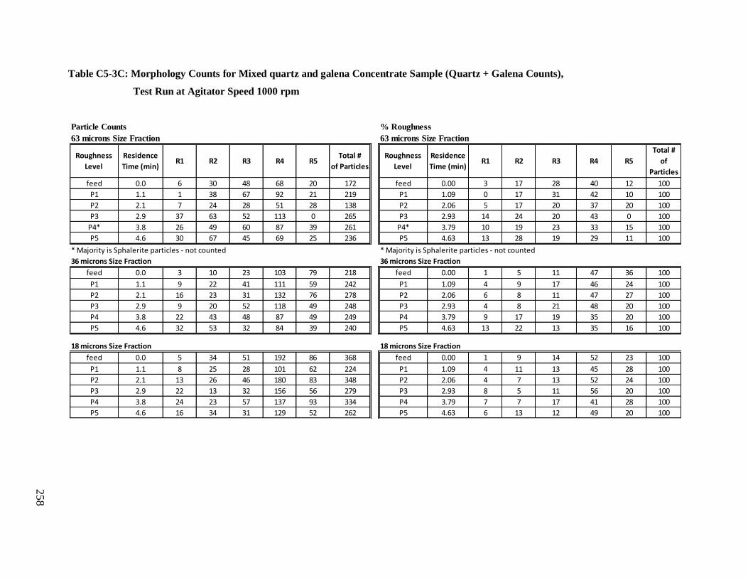
258
Table C5-3C: Morphology Counts for Mixed quartz and galena Concentrate Sample (Quartz + Galena Counts),
Test Run at Agitator Speed 1000 rpm
Particle Counts % Roughness
63 microns Size Fraction 63 microns Size Fraction
Roughness
Level
Residence
Time (min)R1 R2 R3 R4 R5
Total #
of Particles
Roughness
Level
Residence
Time (min)R1 R2 R3 R4 R5
Total #
of
Particles
feed 0.0 6 30 48 68 20 172 feed 0.00 3 17 28 40 12 100
P1 1.1 1 38 67 92 21 219 P1 1.09 0 17 31 42 10 100
P2 2.1 7 24 28 51 28 138 P2 2.06 5 17 20 37 20 100
P3 2.9 37 63 52 113 0 265 P3 2.93 14 24 20 43 0 100
P4* 3.8 26 49 60 87 39 261 P4* 3.79 10 19 23 33 15 100
P5 4.6 30 67 45 69 25 236 P5 4.63 13 28 19 29 11 100
* Majority is Sphalerite particles - not counted * Majority is Sphalerite particles - not counted
36 microns Size Fraction 36 microns Size Fraction
feed 0.0 3 10 23 103 79 218 feed 0.00 1 5 11 47 36 100
P1 1.1 9 22 41 111 59 242 P1 1.09 4 9 17 46 24 100
P2 2.1 16 23 31 132 76 278 P2 2.06 6 8 11 47 27 100
P3 2.9 9 20 52 118 49 248 P3 2.93 4 8 21 48 20 100
P4 3.8 22 43 48 87 49 249 P4 3.79 9 17 19 35 20 100
P5 4.6 32 53 32 84 39 240 P5 4.63 13 22 13 35 16 100
18 microns Size Fraction 18 microns Size Fraction
feed 0.0 5 34 51 192 86 368 feed 0.00 1 9 14 52 23 100
P1 1.1 8 25 28 101 62 224 P1 1.09 4 11 13 45 28 100
P2 2.1 13 26 46 180 83 348 P2 2.06 4 7 13 52 24 100
P3 2.9 22 13 32 156 56 279 P3 2.93 8 5 11 56 20 100
P4 3.8 24 23 57 137 93 334 P4 3.79 7 7 17 41 28 100
P5 4.6 16 34 31 129 52 262 P5 4.63 6 13 12 49 20 100

259
Table C5-4C: Morphology Counts for Mixed quartz and galena Concentrate Sample (Quartz Counts),
Test Run at Agitator Speed 2000 rpm
Particle Counts % Roughness
63 microns Size Fraction 63 microns Size Fraction
Roughness
Level
Residence
Time (min)R1 R2 R3 R4 R5
Total #
of
Particles
Roughness
Level
Residence
Time
(min)
R1 R2 R3 R4 R5
Total #
of
Particles
feed 0.0 4 29 45 61 15 154 feed 0.0 3 19 29 40 10 100
P1 1.1 41 52 55 81 40 269 P1 1.1 15 19 20 30 15 100
P2 2.1 37 52 52 61 11 213 P2 2.1 17 24 24 29 5 100
P3 3.1 41 70 45 77 2 235 P3 3.1 17 30 19 33 1 100
P4 4.2 45 66 64 79 1 255 P4 4.2 18 26 25 31 0 100
P5 5.1 41 67 62 58 1 229 P5 5.1 18 29 27 25 0 100
* mostly broken pieces
36 microns Size Fraction 36 microns Size Fraction
feed 0.0 0 2 3 8 3 16 feed 0.0 0 13 19 50 19 100
P1 1.1 9 38 51 65 12 175 P1 1.1 5 22 29 37 7 100
P2 2.1 10 42 37 54 15 158 P2 2.1 6 27 23 34 9 100
P3 3.1 10 42 57 104 9 222 P3 3.1 5 19 26 47 4 100
P4 4.2 6 31 30 61 6 134 P4 4.2 4 23 22 46 4 100
P5 5.1 11 66 47 93 6 223 P5 5.1 5 30 21 42 3 100
18 microns Size Fraction 18 microns Size Fraction
feed 0.0 0 13 17 55 24 109 feed 0.0 0 12 16 50 22 100
P1 1.1 0 7 16 42 14 79 P1 1.1 0 9 20 53 18 100
P2 2.1 2 15 21 70 21 129 P2 2.1 2 12 16 54 16 100
P3 3.1 4 12 20 60 13 109 P3 3.1 4 11 18 55 12 100
P4 4.2 1 17 39 80 21 158 P4 4.2 1 11 25 51 13 100
P5 5.1 4 12 15 44 14 89 P5 5.1 4 13 17 49 16 100
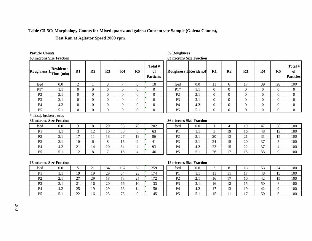
260
Table C5-5C: Morphology Counts for Mixed quartz and galena Concentrate Sample (Galena Counts),
Test Run at Agitator Speed 2000 rpm
Particle Counts % Roughness
63 microns Size Fraction 63 microns Size Fraction
Roughness LevelResidence
Time (min)R1 R2 R3 R4 R5
Total #
of
Particles
Roughness LevelResidence Time (min)R1 R2 R3 R4 R5
Total #
of
Particles
feed 0.0 2 1 3 7 5 18 feed 0.0 11 6 17 39 28 100
P1* 1.1 0 0 0 0 0 0 P1* 1.1 0 0 0 0 0 0
P2 2.1 0 0 0 0 0 0 P2 2.1 0 0 0 0 0 0
P3 3.1 0 0 0 0 0 0 P3 3.1 0 0 0 0 0 0
P4 4.2 0 0 0 0 0 0 P4 4.2 0 0 0 0 0 0
P5 5.1 0 0 0 0 0 0 P5 5.1 0 0 0 0 0 0
* mostly broken pieces
36 microns Size Fraction 36 microns Size Fraction
feed 0.0 3 8 20 95 76 202 feed 0.0 1 4 10 47 38 100
P1 1.1 3 12 10 30 8 63 P1 1.1 5 19 16 48 13 100
P2 2.1 17 11 18 27 13 86 P2 2.1 20 13 21 31 15 100
P3 3.1 10 6 8 15 2 41 P3 3.1 24 15 20 37 5 100
P4 4.2 21 14 20 34 4 93 P4 4.2 23 15 22 37 4 100
P5 5.1 12 8 7 15 4 46 P5 5.1 26 17 15 33 9 100
18 microns Size Fraction 18 microns Size Fraction
feed 0.0 5 21 34 137 62 259 feed 0.0 2 8 13 53 24 100
P1 1.1 19 19 29 84 23 174 P1 1.1 11 11 17 48 13 100
P2 2.1 27 29 18 73 25 172 P2 2.1 16 17 10 42 15 100
P3 3.1 21 16 20 66 10 133 P3 3.1 16 12 15 50 8 100
P4 4.2 25 19 29 63 14 150 P4 4.2 17 13 19 42 9 100
P5 5.1 22 16 25 73 9 145 P5 5.1 15 11 17 50 6 100

261
Table C5-66-12C: Morphology Counts for Mixed quartz and galena Concentrate Sample (Quartz + Galena Counts),
Test Run at Agitator Speed 2000 rpm
Particle Counts % Roughness
63 microns Size Fraction 63 microns Size Fraction
Roughness
Level
Residence
Time (min)R1 R2 R3 R4 R5
Total #
of
Particles
Roughness
Level
Residence
Time (min)R1 R2 R3 R4 R5
Total #
of
Particles
feed 0.0 6 30 48 68 20 172 feed 0.00 3 17 28 40 12 100
P1 1.1 41 52 55 81 40 269 P1 1.11 15 19 20 30 15 100
P2 2.1 37 52 52 61 11 213 P2 2.11 17 24 24 29 5 100
P3 3.1 41 70 45 77 2 235 P3 3.09 17 30 19 33 1 100
P4* 4.2 45 66 64 79 1 255 P4* 4.18 18 26 25 31 0.4 100
P5 5.1 41 67 62 58 1 229 P5 5.08 18 29 27 25 0.4 100
* Majority is Sphalerite particles - not counted * Majority is Sphalerite particles - not counted
36 microns Size Fraction 36 microns Size Fraction
feed 0.0 3 10 23 103 79 218 feed 0.00 1 5 11 47 36 100
P1 1.1 12 50 61 95 20 238 P1 1.11 5 21 26 40 8 100
P2 2.1 27 53 55 81 28 244 P2 2.11 11 22 23 33 11 100
P3 3.1 20 48 65 119 11 263 P3 3.09 8 18 25 45 4 100
P4 4.2 27 45 50 95 10 227 P4 4.18 12 20 22 42 4 100
P5 5.1 23 74 54 108 10 269 P5 5.08 9 28 20 40 4 100
18 microns Size Fraction 18 microns Size Fraction
feed 0.0 5 34 51 192 86 368 feed 0.00 1 9 14 52 23 100
P1 1.1 19 26 45 126 37 253 P1 1.11 8 10 18 50 15 100
P2 2.1 29 44 39 143 46 301 P2 2.11 10 15 13 48 15 100
P3 3.1 25 28 40 126 23 242 P3 3.09 10 12 17 52 10 100
P4 4.2 26 36 68 143 35 308 P4 4.18 8 12 22 46 11 100
P5 5.1 26 28 40 117 23 234 P5 5.08 11 12 17 50 10 100

262
Table C5-1D: Morphology Counts for Lead-Zinc Ore Sample, Test Run at Agitator Speed 1000 rpm
Particle Counts % Roughness
63 microns Size Fraction 63 microns Size Fraction
Roughness
Level
Residence
Time (min)R1 R2 R3 R4 R5
Total #
of
Particles
Roughness
Level
Residence
Time (min)R1 R2 R3 R4 R5
Total #
of
Particles
feed 0.0 36 34 35 86 18 209 feed 0.0 17 16 17 41 9 100
P1 0.7 55 37 46 70 10 218 P1 0.7 25 17 21 32 5 100
P2 1.3 50 67 68 66 5 256 P2 1.3 20 26 27 26 2 100
P3 2.0 74 70 54 80 15 293 P3 2.0 25 24 18 27 5 100
P4 2.6 40 67 44 118 9 278 P4 2.6 14 24 16 42 3 100
P5 3.1 49 96 90 139 10 384 P5 3.1 13 25 23 36 3 100
33 microns Size Fraction 33 microns Size Fraction
feed 0.0 63 40 43 107 22 275 feed 0.0 23 15 16 39 8 100
P1 0.7 53 39 49 73 35 249 P1 0.7 21 16 20 29 14 100
P2 1.3 48 52 40 93 11 244 P2 1.3 20 21 16 38 5 100
P3 2.0 52 61 43 102 14 272 P3 2.0 19 22 16 38 5 100
P4 2.6 56 55 32 88 23 254 P4 2.6 22 22 13 35 9 100
P5 3.1 56 61 39 89 10 255 P5 3.1 22 24 15 35 4 100
16microns Size Fraction 16 microns Size Fraction
feed 0.0 47 21 31 99 48 246 feed 0.0 19 9 13 40 20 100
P1 0.7 57 39 43 106 18 263 P1 0.7 22 15 16 40 7 100
P2 1.3 49 48 30 98 12 237 P2 1.3 21 20 13 41 5 100
P3 2.0 57 46 23 95 6 227 P3 2.0 25 20 10 42 3 100
P4 2.6 65 44 43 101 23 276 P4 2.6 24 16 16 37 8 100
P5 3.1 67 57 41 95 15 275 P5 3.1 24 21 15 35 5 100

263
Table C5-2D: Morphology Counts for Lead-Zinc Ore Sample, Test Run at Agitator Speed 1500 rpm
Particle Counts % Roughness
63 microns Size Fraction 63 microns Size Fraction
Roughness
Level
Residence
Time (min)R1 R2 R3 R4 R5
Total #
of
Particles
Roughness
Level
Residence
Time (min)R1 R2 R3 R4 R5
Total #
of
Particles
feed 0.0 36 34 35 86 18 209 feed 0.0 17 16 17 41 9 100
P1 0.8 19 51 51 88 10 219 P1 0.8 9 23 23 40 5 100
P2 1.7 89 80 44 80 3 296 P2 1.7 30 27 15 27 1 100
P3* 2.4 34 45 41 69 4 193 P3* 2.4 18 23 21 36 2 100
P4 3.2 32 77 92 105 2 308 P4 3.2 10 25 30 34 1 100
P5 3.9 49 85 69 83 2 288 P5 3.9 17 30 24 29 1 100
* mostly broken pieces
33 microns Size Fraction 33 microns Size Fraction
feed 0 63 40 43 107 22 275 feed 0 23 15 16 39 8 100
P1 0.8 69 44 37 92 12 254 P1 0.8 27 17 15 36 5 100
P2 1.7 63 54 42 85 4 248 P2 1.7 25 22 17 34 2 100
P3 2.4 78 54 44 85 7 268 P3 2.4 29 20 16 32 3 100
P4 3.2 45 93 77 113 1 329 P4 3.2 14 28 23 34 0 100
P5 3.9 37 39 48 71 7 202 P5 3.9 18 19 24 35 3 100
* mostly broken pieces
16 microns Size Fraction 16 microns Size Fraction
feed 0 47 21 31 99 48 246 feed 0 19 9 13 40 20 100
P1 0.8 78 62 60 164 25 389 P1 0.8 20 16 15 42 6 100
P2 1.7 58 42 37 80 16 233 P2 1.7 25 18 16 34 7 100
P3 2.4 55 38 51 83 15 242 P3 2.4 23 16 21 34 6 100
P4 3.2 56 42 38 74 6 216 P4 3.2 26 19 18 34 3 100
P5 3.9 39 50 41 77 3 210 P5 3.9 19 24 20 37 1 100

264
Table C5-3D: Morphology Counts for Lead-Zinc Ore Sample, Test Run at Agitator Speed 2000 rpm
Particle Counts % Roughness
63 microns Size Fraction 63 microns Size Fraction
Roughness
Level
Residence
Time (min)R1 R2 R3 R4 R5
Total #
of
Particles
Roughness
Level
Residence
Time (min)R1 R2 R3 R4 R5
Total #
of
Particles
feed 0.0 36 34 35 86 18 209 feed 0.0 17 16 17 41 9 100
P1 0.8 60 67 59 86 0 272 P1 0.8 22 25 22 32 0 100
P2 1.6 70 53 44 120 4 291 P2 1.6 24 18 15 41 1 100
P3 2.3 60 81 58 97 3 299 P3 2.3 20 27 19 32 1 100
P4 3.0 73 93 30 79 4 279 P4 3.0 26 33 11 28 1 100
P5 4.0 0 0 0 0 0 0 P5 4.0 0 0 0 0 0 0
33 microns Size Fraction 33 microns Size Fraction
feed 0.0 63 40 43 107 22 275 feed 0.0 23 15 16 39 8 100
P1 0.8 45 37 33 66 2 183 P1 0.8 25 20 18 36 1 100
P2 1.6 75 44 60 77 5 261 P2 1.6 29 17 23 30 2 100
P3 2.3 59 50 43 75 7 234 P3 2.3 25 21 18 32 3 100
P4 3.0 0 0 0 0 0 0 P4 3.0 0 0 0 0 0 0
P5 4.0 0 0 0 0 0 0 P5 4.0 0 0 0 0 0 0
16 microns Size Fraction 16 microns Size Fraction
feed 0.0 47 21 31 99 48 246 feed 0.0 19 9 13 40 20 100
P1 0.8 71 42 42 111 17 283 P1 0.8 25 15 15 39 6 100
P2 1.6 106 69 92 119 23 409 P2 1.6 26 17 22 29 6 100
P3 2.3 80 38 40 95 6 259 P3 2.3 31 15 15 37 2 100
P4 3.0 66 52 35 84 15 252 P4 3.0 26 21 14 33 6 100
P5 4.0 88 61 44 106 13 312 P5 4.0 28 20 14 34 4 100

265
Appendix C6: List of Morphology Samples
UBC Morpholgy Study - Samples
Reem Roufail (PhD candidate)Q = Quartz
G = Galena
M = Mixed Sample of Silica and Galena
O = Ore Sample from Red SAG Discharge (Pb-Zn circuit)
Sample Size Fraction Availability Sample Size Fraction Availability Sample Size Fraction Availability Sample Size Fraction Availability
Q-feed 53 micron G-feed 53 micron M-feed 53 micron O-feed 53 micron
C3 (27 micron) C1 (26 micron) C2 (31 micron) C2 (28 micron)
C5 (13 micron) C3 (14 micron) C4 (14 mircon) C4 (13 micron)
Q1000-P1 53 mircon G1000-P1 C2 (31 micron) M1000-P1 53 mircon O1000-P1 53 micron
C3 (27 micron) C1 (26 mircon) C2 (31 micron) C2 (28 micron)
C5 (13 micron) C3 (14 mircon) C4 (14 mircon) C4 (13 micron)
Q1000-P2 53 mircon G1000-P2 53 mircon M1000-P2 53 mircon O1000-P2 53 micron
C3 (27 micron) C1 (26 mircon) C2 (31 micron) C2 (28 micron)
C5 (13 micron) C3 (14 mircon) C4 (14 mircon) C4 (13 micron)
Q1000-P3 53 mircon G1000-P3 53 mircon M1000-P3 53 mircon O1000-P3 53 micron
C3 (27 micron) C1 (26 mircon) C2 (31 micron) C2 (28 micron)
C5 (13 micron) C3 (14 mircon) C4 (14 mircon) C4 (13 micron)
Q1000-P4 53 mircon G1000-P4 53 mircon M1000-P4 53 mircon O1000-P4 53 micron
C3 (27 micron) C1 (26 mircon) C2 (31 micron) C2 (28 micron)
C5 (13 micron) C3 (14 mircon) C4 (14 mircon) C4 (13 micron)
Q1000-5 53 mircon G1000-5 53 mircon M1000-5 53 mircon O1000-5 53 micron
C3 (27 micron) C1 (26 mircon) C2 (31 micron) C2 (28 micron)
C5 (13 micron) C3 (14 mircon) C4 (14 mircon) C4 (13 micron)
Q1500-P1 53 mircon G1500-P1 53 mircon M2000-P1 53 mircon O1500-P1 53 micron
C3 (27 micron) C1 (26 mircon)* C2 (31 micron) C2 (28 micron)
C5 (13 micron) C3 (14 mircon) C4 (14 mircon) C4 (13 micron)
Q1500-P2 53 mircon G1500-P2 53 mircon M2000-P2 53 mircon * O1500-P2 53 micron
C3 (27 micron) C1 (26 mircon)* C2 (31 micron) C2 (28 micron)
C5 (13 micron) C3 (14 mircon) C4 (14 mircon) C4 (13 micron)
Q1500-P3 53 mircon G1500-P3 53 mircon M2000-P3 53 mircon * O1500-P3 53 micron
C3 (27 micron) C1 (26 mircon)* C2 (31 micron)* C2 (28 micron)
C5 (13 micron) C3 (14 mircon) C4 (14 mircon) C4 (13 micron)
Q1500-P4 53 mircon G1500-P4 53 mircon M2000-P4 53 mircon * O1500-P4 53 micron
C3 (27 micron) C1 (26 mircon)combined
with C2 C2 (31 micron)* C2 (28 micron)
C5 (13 micron) C3 (14 mircon) C4 (14 mircon) C4 (13 micron)
Q1500-5 53 mircon G1500-5 53 mircon M2000-5 53 mircon * O1500-P5 53 micron
C3 (27 micron) C1 (26 mircon)*combined
with C2 C2 (31 micron)* C2 (28 micron)
C5 (13 micron) C3 (14 mircon) C4 (14 mircon) C4 (13 micron)

266
Sample Size Fraction Availability Sample Size Fraction Availability Sample Size Fraction Availability Sample Size Fraction Availability
Q2000-P1 53 mircon G2000-P1 53 mircon O2000-P1 53 micron
C3 (27 micron) C1 (26 mircon)* C2 (28 micron)
C5 (13 micron) C3 (14 mircon) C4 (13 micron)
Q2000-P2 53 mircon G2000-P2 53 mircon O2000-P2 53 micron
C3 (27 micron) C1 (26 mircon)* C2 (28 micron)
C5 (13 micron) C3 (14 mircon) C4 (13 micron)
Q2000-P3 53 mircon G2000-P3 53 mircon O2000-P3 53 micron
C3 (27 micron) C1 (26 mircon)combined
with C2 C2 (28 micron)
C5 (13 micron) C3 (14 mircon) C4 (13 micron)
Q2000-P4 53 mircon G2000-P4 53 mircon O2000-P4 53 micron
C3 (27 micron) C1 (26 mircon)combined
with C2 C2 (28 micron)
C5 (13 micron) C3 (14 mircon) C4 (13 micron)*
Q2000-5 53 mircon G2000-5 53 mircon O2000-P5 53 micron
C3 (27 micron) C1 (26 mircon)combined
with C2 C2 (28 micron)
C5 (13 micron) C3 (14 mircon) C4 (13 micron)*
Note:
* Total Number of Samples are 169 that need Morphology Analysis
* Orange Stars and ALL Ore samples are all that we have i.e. No more Samples
: Not generated


