
The Artifact Subspace Reconstruction method
Christian A Kothe
SCCN / INC / UCSD
January 2013

Artifact Subspace Reconstruction
• New algorithm to remove non-stationary high-variance signals from EEG
• Reconstructs the missing data using a spatial mixing matrix (assuming volume conduction)
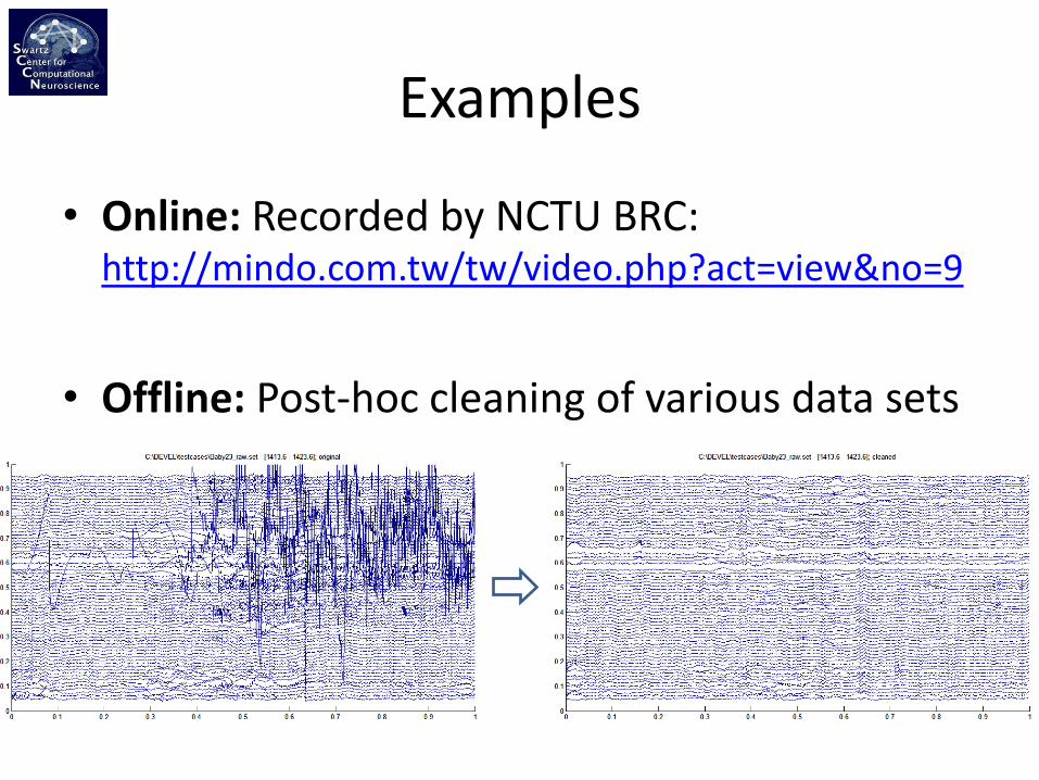
Examples
• Online: Recorded by NCTU BRC: http://mindo.com.tw/tw/video.php?act=view&no=9
• Offline: Post-hoc cleaning of various data sets
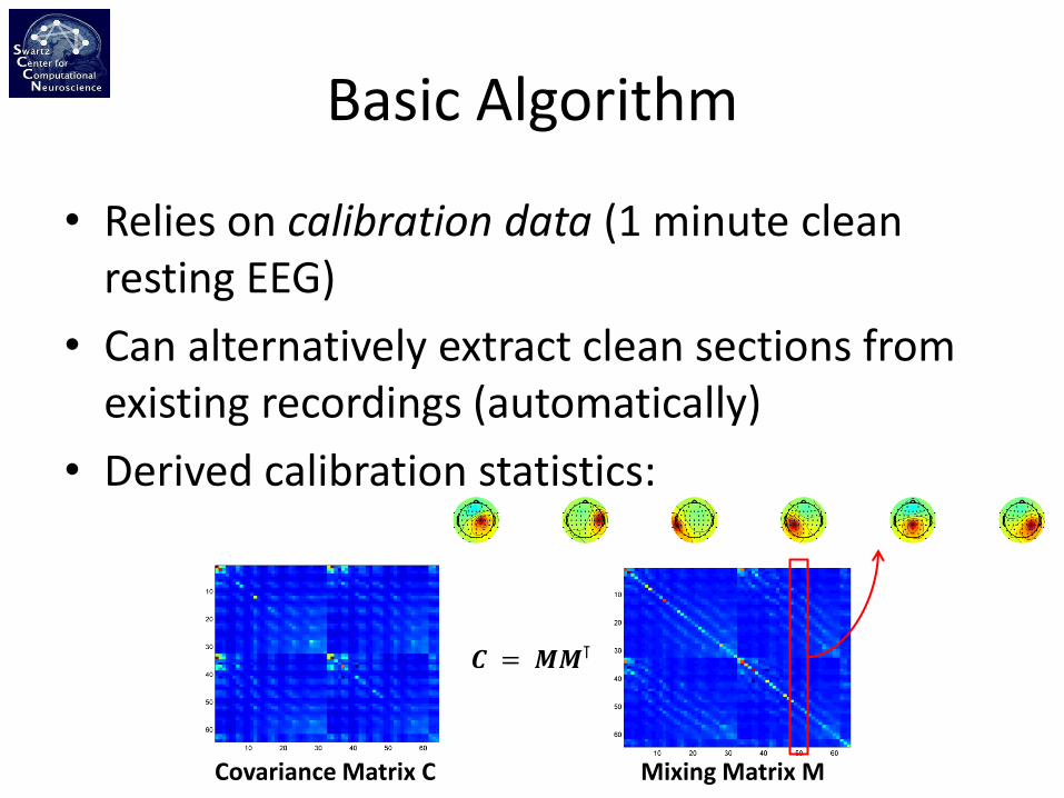
Basic Algorithm
• Relies on calibration data (1 minute clean resting EEG)
• Can alternatively extract clean sections from existing recordings (automatically)
• Derived calibration statistics:
Covariance Matrix C Mixing Matrix M
𝑪 = 𝑴𝑴⊺

Robust Statistics
• Calibration statistics are estimated in a robust manner (to minimize any effect of artifacts)
• Using the Geometric Median 𝓖 over windowed (1-second) estimates:
• Note: Also a very good drop-in replacement for outlier-sensitive averages in a wide range of statistical procedures (e.g., ICA updates)!
𝓖 𝑿 = argmin𝒚 𝒙𝑖 − 𝒚 2
𝑚
𝑖=1
Geometric Median
𝑦𝑖+1 = 𝑥𝑗
𝑥𝑗 − 𝑦𝑖
𝑚
𝑗=1
1
𝑥𝑗 − 𝑦𝑖
𝑚
𝑗=1
Iterative Formula (iteratively reweighted least squares)

Robust Statistics
• Geometric Median over covariance matrices is not the ideal measure (since covariance matrices lie on a curved manifold)
• Can re-parameterize into Cholesky factorizations, take median there, then back-transform:
Covariance Matrix Cholesky Factorization
(median of upper-triangular
matrices is still upper-triangular)
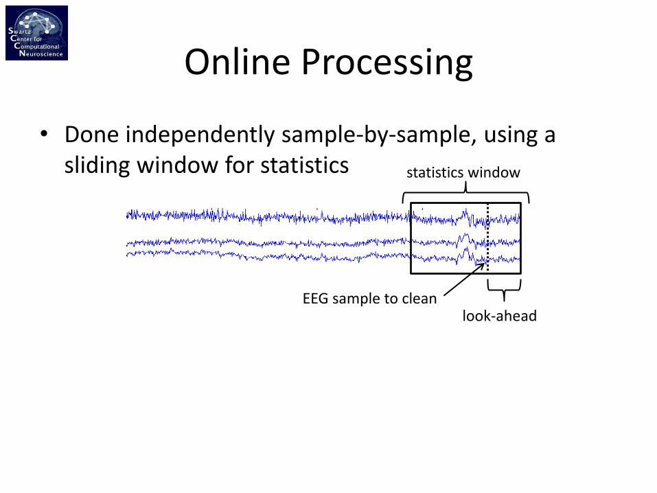
Online Processing
• Done independently sample-by-sample, using a sliding window for statistics
statistics window
EEG sample to clean look-ahead
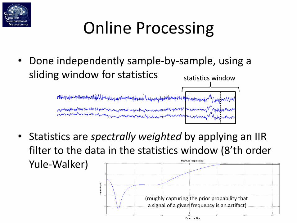
Online Processing
• Done independently sample-by-sample, using a sliding window for statistics
• Statistics are spectrally weighted by applying an IIR filter to the data in the statistics window (8’th order Yule-Walker)
statistics window
(roughly capturing the prior probability that a signal of a given frequency is an artifact)

Online Processing
• Step 2: Separate high-amplitude signal components (potential artifact components) in the statistics window from other components
• Done using Principal Component Analysis (PCA) on a sliding window:
Random sample of high-variance components
PCA Solution 𝑽 = 𝐞𝐢𝐠(𝑾𝑾⊺)
Raw Signal Window W (spectrally filtered)
Online Processing
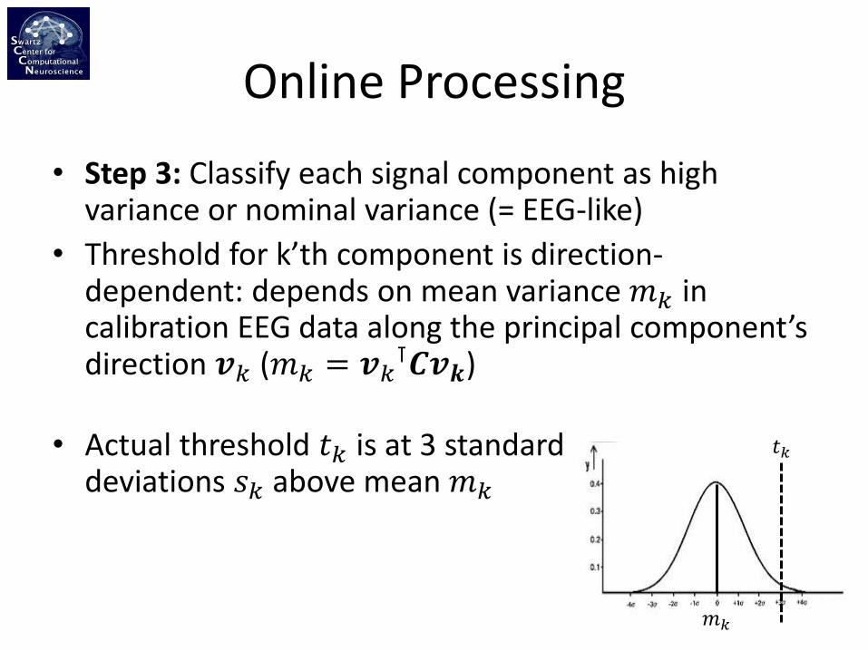
• Step 3: Classify each signal component as high variance or nominal variance (= EEG-like)
• Threshold for k’th component is direction-dependent: depends on mean variance 𝑚𝑘 in calibration EEG data along the principal component’s direction 𝒗𝑘 (𝑚𝑘 = 𝒗𝑘
⊺𝑪𝒗𝒌)
• Actual threshold 𝑡𝑘 is at 3 standard deviations 𝑠𝑘 above mean 𝑚𝑘 (𝑠𝑘 is deduced from 𝑚𝑘 using a 𝜒2 assumption under which these parameters are functionally related)
𝑡𝑘
𝑚𝑘

Online Processing
• Step 3: Classify each signal component as high variance or nominal variance (= EEG-like)
• Threshold for k’th component is direction-dependent: depends on mean variance 𝑚𝑘 in calibration EEG data along the principal component’s direction 𝒗𝑘 (𝑚𝑘 = 𝒗𝑘
⊺𝑪𝒗𝒌)
• Actual threshold 𝑡𝑘 is at 3 standard deviations 𝑠𝑘 above mean 𝑚𝑘 (𝑠𝑘 is deduced from 𝑚𝑘 using a 𝜒2 assumption under which these parameters are functionally related)
window length in s
𝒔 𝒌/𝒎𝒌
Online Processing
• Step 4: Reconstruct content of high-variance subspace from content of nominal-variance subspace (i.e., estimate missing data)
• Basic idea: EEG is highly correlated; can estimate content of one channel based on its neighbors
• The same works not just for a channel but also for a linear combination of channels (e.g., sum or difference of 2), i.e., can estimate content of artifact subspace from non-artifact subspace
Geometric Approach
• Mixing matrix M represents linear mapping from orthog. latent components L onto sensors S: 𝑺 = 𝑴𝑳
• Component activation can be estimated as 𝑳 = 𝑴−𝟏𝑺 (but fails to keep artifacts out of L)
• To estimate a clean L, the inverse of a truncated mixing matrix (artifact channels zeroed out) can be used: 𝑴𝒕𝒓𝒖𝒏𝒄 = 𝑴 ∘ 𝑻,
𝑳 = 𝑴𝒕𝒓𝒖𝒏𝒄+𝑺
(Note: here we frame it in terms of channels, moving to components later)

Geometric Approach
• Given a clean estimate of L, can back-project onto channels again using the full M:
𝑺𝒄𝒍𝒆𝒂𝒏 = 𝑴 𝑴 ∘ 𝑻+𝑺
• Doing the same in artifact/non-artifact principal component space V requires a rotation into V, followed by back-rotation:
𝑺𝒄𝒍𝒆𝒂𝒏 = 𝑽𝑴𝑽 𝑴𝑽 ∘ 𝑻+𝑽⊺𝑺
• … using a rotated mixing matrix 𝑴𝑽 = 𝑽⊺𝑴
• All steps can be baked into a re-projection matrix R so 𝑺𝒄𝒍𝒆𝒂𝒏 = RS:
𝑹 = 𝑴 𝑽⊺𝑴 ∘ 𝑻 +𝑽⊺
A
.
.
.
.
.
.
Sensor Channels S Latent Components L

Geometric Approach
• Given a clean estimate of L, can back-project onto channels again using the full M:
𝑺𝒄𝒍𝒆𝒂𝒏 = 𝑴 𝑴 ∘ 𝑻+𝑺
• Doing the same in artifact/non-artifact principal component space V requires a rotation into V, followed by back-rotation:
𝑺𝒄𝒍𝒆𝒂𝒏 = 𝑽𝑴𝑽 𝑴𝑽 ∘ 𝑻+𝑽⊺𝑺
• … using a rotated mixing matrix 𝑴𝑽 = 𝑽⊺𝑴
• All steps can be baked into a re-projection matrix R such that 𝑺𝒄𝒍𝒆𝒂𝒏 = RS:
𝑹 = 𝑴 𝑽⊺𝑴 ∘ 𝑻 +𝑽⊺

Speed-up
• Calculate reprojection matrix R for every n’th sample (n=32)
• Then interpolate R for intermediate samples (using a raised-cosine window)
• Runs in real time on up to 256 channels
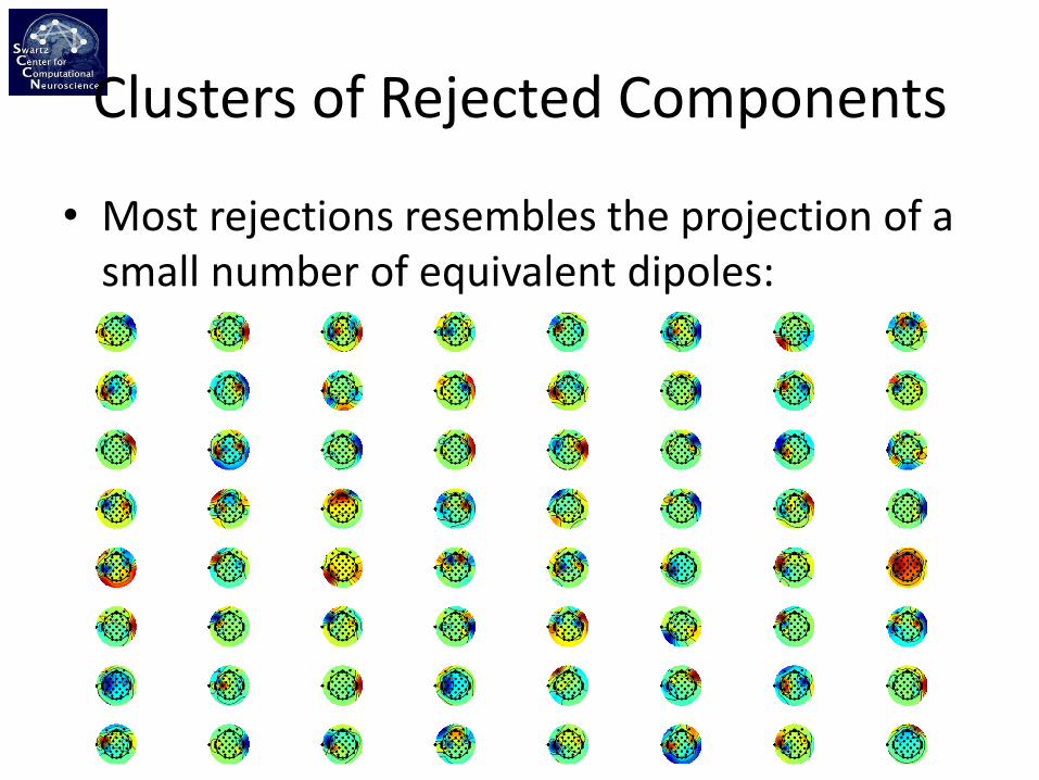
Clusters of Rejected Components
• Most rejections resembles the projection of a small number of equivalent dipoles:


