Template Attacks on Different Devices

Omar Choudary and Markus G. Kuhn

Computer Laboratory, University of Cambridge, Cambridge, UK{omar.choudary,markus.kuhn}@cl.cam.ac.uk

Abstract. Template attacks remain a most powerful side-channel tech-nique to eavesdrop on tamper-resistant hardware. They use a profilingstep to compute the parameters of a multivariate normal distributionfrom a training device and an attack step in which the parameters ob-tained during profiling are used to infer some secret value (e.g. crypto-graphic key) on a target device. Evaluations using the same device forboth profiling and attack can miss practical problems that appear whenusing different devices. Recent studies showed that variability caused bythe use of either different devices or different acquisition campaigns onthe same device can have a strong impact on the performance of tem-plate attacks. In this paper, we explore further the effects that lead tothis decrease of performance, using four different Atmel XMEGA 256A3U 8-bit devices. We show that a main difference between devices is aDC offset and we show that this appears even if we use the same devicein different acquisition campaigns. We then explore several variants ofthe template attack to compensate for these differences. Our results showthat a careful choice of compression method and parameters is the keyto improving the performance of these attacks across different devices.In particular we show how to maximise the performance of templateattacks when using Fisher’s Linear Discriminant Analysis or PrincipalComponent Analysis. Overall, we can reduce the entropy of an unknown8-bit value below 1.5 bits even when using different devices.

Keywords: Side-channel attacks · Template attacks · Multivariateanalysis

1 Introduction

Side-channel attacks are powerful tools for inferring secret algorithms or data(passwords, cryptographic keys, etc.) processed inside tamper-resistant hard-ware, if an attacker can monitor a channel leaking such information, most no-tably the power-supply current and unintended electromagnetic emissions.

One of the most powerful side-channel attacks is the template attack [2],which consists of a profiling step to compute some parameters (the templates)on a training device and an attack step in which the templates are used toinfer some secret data on a target device (Section 2). However, most previousstudies [2,5,8,10,17] used the same device (and possibly acquisition campaign)for the profiling and attack phases. Only recently, Renauld et al. [12] performed

E. Prouff (Ed.): COSADE 2014, LNCS 8622, pp. 179–198, 2014.The final publication is available at Springer via http://dx.doi.org/10.1007/978-3-319-10175-0_13

an extensive study on 20 different devices, showing that the template attack maynot work at all when the profiling and attack steps are performed on differentdevices; Elaabid et al. [14] showed that acquisition campaigns on the same device,but conducted at different times, also lead to worse template-attack results; andLomne et al. [16] evaluated this scenario using electromagnetic leakage.

In this paper, we explore further the causes that make template attacksperform worse across different devices. For this purpose, we evaluate the templateattacks with four different Atmel XMEGA 256 A3U 8-bit devices, using differentcompression methods and parameters.

We show that, for our experiments, a main difference across devices and ac-quisition campaigns is a DC offset, and this difference decreases very much theperformance of template attacks (Section 4). To compensate for differences be-tween devices or campaigns we evaluate several variants of the template attack(Section 5). One of them needs multiple profiling devices, but can improve sig-nificantly the performance of template attacks when using sample selection asthe compression method (Section 5.3). However, based on detailed analysis ofFisher’s Linear Discriminant Analysis (LDA) and Principal Component Analy-sis (PCA), we explain how to use these compression techniques to maximise theperformance of template attacks on different devices, even when profiling on asingle device (Section 5.4).

Overall, our results show that a good choice of compression method and pa-rameters can dramatically improve template attacks across different devices oracquisition campaigns. Previous studies [12,14] may have missed this by evalu-ating only one compression method.

2 Template Attacks

To implement a template attack, we need physical access to a pair of devicesof the same model, which we refer to as the profiling and the attacked device.We wish to infer some secret value k? ∈ S, processed by the attacked device atsome point. For an 8-bit microcontroller, S = {0, . . . , 255} might be the set ofpossible byte values manipulated by a particular machine instruction.

We assume that we determined the approximate moments of time when thesecret value k? is manipulated and we are able to record signal traces (e.g.,supply current or electromagnetic waveforms) around these moments. We referto these traces as leakage vectors. Let {t1, . . . , tmr} be the set of time samplesand xr ∈ Rmr

be the random vector from which leakage traces are drawn.During the profiling phase we record np leakage vectors xr

ki ∈ Rmr

from theprofiling device for each possible value k ∈ S, and combine these as row vectorsxrki′ in the leakage matrix Xr

k ∈ Rnp×mr

.1

Typically, the raw leakage vectors xrki provided by the data acquisition device

contain a very large number mr of samples (random variables), due to high sam-pling rates used. Therefore, we might compress them before further processing,

1 Throughout this paper x′ is the transpose of x.

2

either by selecting only a subset of m � mr of those samples, or by applyingsome other data-dimensionality reduction method, such as Principal ComponentAnalysis (PCA) or Fisher’s Linear Discriminant Analysis (LDA).

We refer to such compressed leakage vectors as xki ∈ Rm and combine all ofthese as rows into the compressed leakage matrix Xk ∈ Rnp×m . (Without anysuch compression step, we would have Xk = Xr

k and m = mr.)Using Xk we can compute the template parameters xk ∈ Rm and Sk ∈

Rm×m for each possible value k ∈ S as

xk = 1np

np∑i=1

xki, Sk = 1np−1

np∑i=1

(xki − xk)(xki − xk)′, (1)

where the sample mean xk and the sample covariance matrix Sk are the estimatesof the true mean µk and true covariance Σk. Note that

np∑i=1

(xki − xk)(xki − xk)′

= X′kXk, (2)

where Xk is Xk with x′k subtracted from each row, and the latter form allowsfast vectorised computation of the covariance matrices in (1).

In our experiments we observed that the particular covariance matrices Sk

are very similar and seem to be independent of the candidate k. In this case, asexplained in a previous paper [17], we can use a pooled covariance matrix

Spooled =1

|S|(np − 1)

∑k∈S

np∑i=1

(xki − xk)(xki − xk)′, (3)

to obtain a much better estimate of the true covariance matrix Σ.In the attack phase, we try to infer the secret value k? ∈ S processed by the

attacked device. We obtain na leakage vectors xi ∈ Rm from the attacked device,using the same recording technique and compression method as in the profilingphase, resulting in the leakage matrix Xk? ∈ Rna×m . Then, using Spooled, wecan compute a linear discriminant score [17], namely

djointLINEAR(k | Xk?) = x′kS−1

pooled

( ∑xi∈Xk?

xi

)− na

2x′kS−1

pooledxk, (4)

for each k ∈ S, and try all k ∈ S on the attacked device, in order of decreasingscore (optimized brute-force search, e.g. for a password or cryptographic key),until we find the correct k?.

2.1 Guessing Entropy

In this work we are interested in evaluating the overall practical success of thetemplate attacks when using different devices. For this purpose we use the guess-ing entropy, which estimates the (logarithmic) average cost of an optimized

3

brute-force search. The guessing entropy gives the expected number of bits ofuncertainty remaining about the target value k?, by averaging the results of theattack over all k? ∈ S. The lower the guessing entropy, the more successful theattack has been and the less effort remains to search for the correct k?. We com-pute the guessing entropy g as shown in our previous work [17]. For all the resultsshown in this paper, we compute the guessing entropy on 10 random selectionsof traces Xk? and plot the average guessing entropy over these 10 iterations.

2.2 Compression Methods

Previously [17], we provided a detailed comparison of the most common compres-sion methods: sample selection (1ppc, 3ppc, 20ppc, allap), Principal ComponentAnalysis (PCA) and Fisher’s Linear Discriminant Analysis (LDA), which wesummarise here. For the sample selection methods 1ppc, 3ppc, 20ppc and allap,we first compute a signal-strength estimate s(t) for each sample j ∈ {1, . . . ,mr},by summing the absolute differences2 between the mean vectors xr

k, and then se-lect the 1 sample per clock cycle (1ppc, 6 ≤ m ≤ 10), 3 samples per clock cycle(3ppc , 18 ≤ m ≤ 30), 20 samples per clock cycle (20ppc, 75 ≤ m ≤ 79)or the 5% samples (allap, m = 125) having the largest s(t). For PCA, wefirst combine the first m eigenvectors uj ∈ Rmr

of the between-groups ma-trix B =

∑k∈S(xr

k − xr)(xrk − xr)

′, where xr = 1

|S|∑

k∈S xrk, into the matrix

of eigenvectors U = [u1, . . . ,um], and then we project the raw leakage matri-ces Xr

k into a lower-dimensional space as Xk = XrkU. For LDA, we use the

matrix B and the pooled covariance Spooled from (3), computed from the un-compressed traces xr

i, and combine the eigenvectors aj ∈ Rmr

of S−1pooledB into

the matrix A = [a1, . . . ,am]. Then, we use the diagonal matrix Q ∈ Rm×m , with

Qjj = (aj′Spooledaj)

− 12 , to scale the matrix of eigenvectors A and use U = AQ

to project the raw leakage matrices as Xk = XrkU. In this case, the compressed

covariances Sk ∈ Rm×m and Spooled ∈ Rm×m reduce to the identity matrix I,resulting in more efficient template attacks.

For most of the results shown in Sections 4 and 5, we used PCA and LDAwith m = 4, based on the elbow rule (visual inspection of eigenvalues) derivedfrom a standard implementation of PCA and LDA. However, as we will thenshow in Section 5.4, a careful choice of m is the key to good results.

2.3 Standard Method

Using the definitions from the previous sections, we can define the followingstandard method for implementing template attacks.

Method 1 (Standard)

1. Obtain the np leakage traces in Xk from the profiling device, for each k.2. Compute the template parameters (xk,Spooled) using (1) and (3).3. Obtain the leakage traces Xk? from the attacked device.4. Compute the guessing entropy as described in Section 2.1.

2 The SNR signal-strength estimate generally provided similar results (omitted here).

4

3 Evaluation Setup

For our experimental research we produced four custom PCBs (named Alpha,Beta, Gamma and Delta) for the unprotected 8-bit Atmel XMEGA 256 A3U mi-crocontroller. The current consumption across all CPU ground pins is measuredthrough a single 10-ohm resistor. We powered the devices from a battery via a3.3 V linear regulator and supplied a 1 MHz sine wave clock signal. We used aTektronix TDS 7054 8-bit oscilloscope with P6243 active probe, at 250 MS/s,with 500 MHz bandwidth in SAMPLE mode. Devices Alpha and Beta used aCPU with week batch ID 1145, while Gamma and Delta had 1230.

For the analysis presented in this paper we run five acquisition campaigns:one for each of the devices, which we call Alpha, Beta, Gamma and Delta (i.e.the same name as the device), and another one at a later time for Beta, which wecall Beta Bis. For all the acquisition campaigns we used the settings describedabove. Then, for each campaign and each candidate value k ∈ {0, . . . , 255} werecorded 3072 traces xr

ki (i.e., 786 432 traces per acquisition campaign), which werandomly divided into a training set (for the profiling phase) and an evaluationset (for the attack phase). Each acquisition campaign took about 2 hours. Wenote a very important detail for our experiments: instead of acquiring all thetraces per k sequentially (i.e. first the 3072 traces for k = 0, then 3072 tracesfor k = 1, and so on), we used random permutations of all the 256 values k andacquired 256 traces at a time (corresponding to a random permutation of allthe 256 values k), for a total of 3072 iterations. This method distributes equallyany external noise (e.g. due to temperature variation) across the traces of all thevalues k. As a result, the covariances Sk will be similar and the mean vectorsxk will be affected in the same manner so they will not be dependent on factorssuch as low-frequency temperature variation.

For all the results shown in this paper we used np = 1000 traces xrki per

candidate k during the profiling phase. Each trace contains mr = 2500 sam-ples, recorded while the target microcontroller executed the same sequence ofinstructions loaded from the same addresses: a MOV instruction, followed byseveral LOAD instructions. All the LOAD instructions require two clock cyclesto transfer a value from RAM into a register, using indirect addressing. In allthe experiments our goal was to determine the success of the template attacks inrecovering the byte k processed by the second LOAD instruction. All the otherinstructions were processing the value zero, meaning that in our traces none ofthe variability should be caused by variable data in other nearby instructionsthat may be processed concurrently in various pipeline stages. This approach,also used in other studies [8,13,17], provides a general setting for the evaluationof the template attacks. Specific algorithm attacks (e.g. on the S-box output ofa block cipher such as AES) may be mounted on top of this.

4 Ideal vs Real Scenario

Most publications on template attacks [2,5,8,10,17] used the same device (andmost probably the same acquisition campaign) for the profiling and attack phase

5

100

101

102

103

0

1

2

3

4

5

6

na (log axis)

Gue

ssin

g en

trop

y (b

its)

LDA, m=4PCA, m=4sample, 1ppcsample, 3ppcsample, 20ppcsample, allap

100

101

102

103

0

1

2

3

4

5

6

na (log axis)

Gue

ssin

g en

trop

y (b

its)

100

101

102

103

0

1

2

3

4

5

6

na (log axis)

Gue

ssin

g en

trop

y (b

its)

100

101

102

103

0

1

2

3

4

5

6

na (log axis)

Gue

ssin

g en

trop

y (b

its)

LDA, m=4PCA, m=4sample, 1ppcsample, 3ppcsample, 20ppcsample, allap

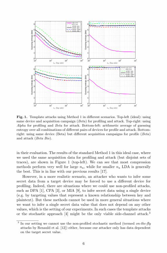
Fig. 1. Template attacks using Method 1 in different scenarios. Top-left (ideal): usingsame device and acquisition campaign (Beta) for profiling and attack. Top-right: usingAlpha for profiling and Beta for attack. Bottom-left: arithmetic average of guessingentropy over all combinations of different pairs of devices for profile and attack. Bottom-right: using same device (Beta) but different acquisition campaigns for profile (Beta)and attack (Beta Bis).

in their evaluation. The results of the standard Method 1 in this ideal case, wherewe used the same acquisition data for profiling and attack (but disjoint sets oftraces), are shown in Figure 1 (top-left). We can see that most compressionmethods perform very well for large na, while for smaller na LDA is generallythe best. This is in line with our previous results [17].

However, in a more realistic scenario, an attacker who wants to infer somesecret data from a target device may be forced to use a different device forprofiling. Indeed, there are situations where we could use non-profiled attacks,such as DPA [1], CPA [3], or MIA [9], to infer secret data using a single device(e.g. by targeting values that represent a known relationship between key andplaintext). But these methods cannot be used in more general situations wherewe want to infer a single secret data value that does not depend on any othervalues, which is the setting of our experiments. In such cases the template attacksor the stochastic approach [4] might be the only viable side-channel attack.3

3 In our setting we cannot use the non-profiled stochastic method (termed on-the-flyattacks by Renauld et al. [12]) either, because our attacker only has data dependenton the target secret value.

6

Moreover, the template attacks are expected to perform better than the otherattacks when provided with enough profiling data [11]. Therefore, we would liketo use template attacks also with different devices for profiling and attack.

As we show in Figure 1 (top-right), the efficacy of template attacks usingthe standard Method 1 drops dramatically when using different devices for theprofiling and attack steps. This was also observed by Renauld et al. [12], bytesting the success of template attacks on 20 different devices with 65 nm CMOStransistor technology. Moreover, Elaabid et al. [14] mentioned that even if theprofiling and attack steps are performed on the same device but on differentacquisition campaigns we will also observe weak success of the template attacks.In Figure 1 (bottom-right) we confirm that indeed, even when using the samedevice but different acquisition campaigns (same acquisition settings), we getresults as bad or even worse as when using different devices. In Section 5, weoffer an explanation for why LDA can perform well across different devices.

4.1 Causes of trouble

In order to explore the causes that lead to worse attack performance on differentacquisition campaigns, we start by looking at two measures of standard deviation(std), that we call std devices and std data.

Let x(i)kj be the mean value of sample j ∈ {1, . . . ,m} for the candidate

k ∈ S on the campaign i ∈ {1, . . . , nc}, x(i)j = 1

|S|∑

k∈S x(i)kj , zk(j) = [(x

(1)kj −

x(1)j ), . . . , (x

(nc)kj − x

(nc)j )] = [z

(1)k (j), . . . , z

(nc)k (j)] and zk(j) = 1

nc

∑nc

i=1 z(i)k (j).

Then,

std devices(j) =1

|S|∑k∈S

√√√√ 1

nc − 1

nc∑i=1

(z(i)k (j)− zk(j))

2, (5)

and

std data(j) =1

nc

nc∑i=1

√1

|S| − 1

∑k∈S

(x(i)kj − x

(i)j )

2. (6)

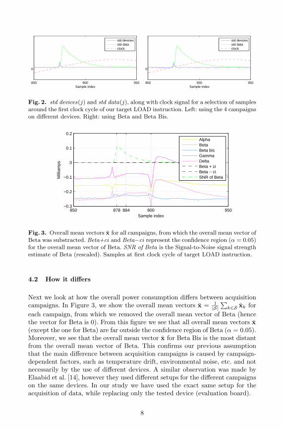
We show these values in Figure 2. The results on the left plot are from the fourcampaigns on different devices, while the results on the right plot are from thetwo campaigns on the device Beta. We can observe that both plots are verysimilar, which suggests that the differences between campaigns are not entirelydue to different devices being used, but largely due to different sources of noise(e.g., temperature, interference, etc.) that may affect in a particular mannereach acquisition campaign. Using a similar type of plots, Renauld et al. [12,Fig. 1] observed a much stronger difference, attributed to physical variability.Their observed differences are not evident in our experiments, possibly becauseour devices use a larger transistor size (around 0.12 µm)4.

4 See http://www.avrfreaks.net/?name=PNphpBB2&file=viewtopic&p=976590.

7

850 900 950

0

Sample index

std devicesstd dataclock

850 900 950

0

Sample index

std devicesstd dataclock

Fig. 2. std devices(j) and std data(j), along with clock signal for a selection of samplesaround the first clock cycle of our target LOAD instruction. Left: using the 4 campaignson different devices. Right: using Beta and Beta Bis.

850 878 884 900 950−0.3

−0.2

−0.1

0

0.1

0.2

Sample index

Mill

iam

ps

AlphaBetaBeta bisGammaDeltaBeta + ciBeta − ciSNR of Beta

Fig. 3. Overall mean vectors x for all campaigns, from which the overall mean vector ofBeta was substracted. Beta+ci and Beta−ci represent the confidence region (α = 0.05)for the overall mean vector of Beta. SNR of Beta is the Signal-to-Noise signal strengthestimate of Beta (rescaled). Samples at first clock cycle of target LOAD instruction.

4.2 How it differs

Next we look at how the overall power consumption differs between acquisitioncampaigns. In Figure 3, we show the overall mean vectors x = 1

|S|∑

k∈S xk for

each campaign, from which we removed the overall mean vector of Beta (hencethe vector for Beta is 0). From this figure we see that all overall mean vectors x(except the one for Beta) are far outside the confidence region of Beta (α = 0.05).Moreover, we see that the overall mean vector x for Beta Bis is the most distantfrom the overall mean vector of Beta. This confirms our previous assumptionthat the main difference between acquisition campaigns is caused by campaign-dependent factors, such as temperature drift, environmental noise, etc. and notnecessarily by the use of different devices. A similar observation was made byElaabid et al. [14], however they used different setups for the different campaignson the same devices. In our study we have used the exact same setup for theacquisition of data, while replacing only the tested device (evaluation board).

8

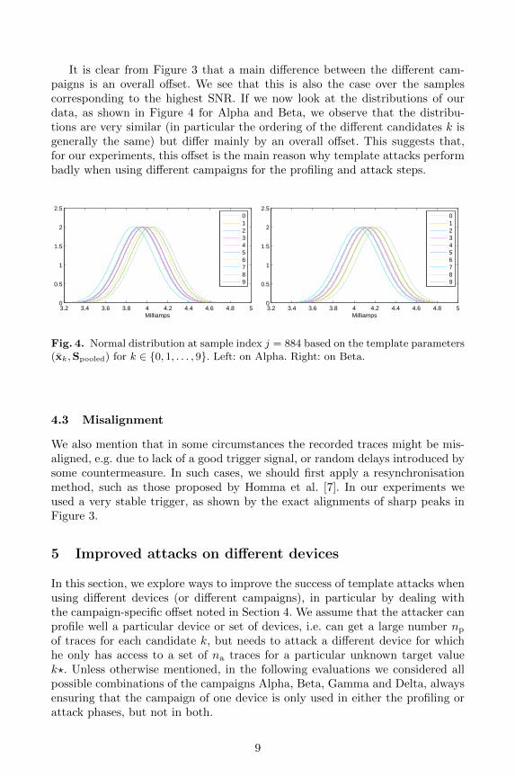
It is clear from Figure 3 that a main difference between the different cam-paigns is an overall offset. We see that this is also the case over the samplescorresponding to the highest SNR. If we now look at the distributions of ourdata, as shown in Figure 4 for Alpha and Beta, we observe that the distribu-tions are very similar (in particular the ordering of the different candidates k isgenerally the same) but differ mainly by an overall offset. This suggests that,for our experiments, this offset is the main reason why template attacks performbadly when using different campaigns for the profiling and attack steps.

3.2 3.4 3.6 3.8 4 4.2 4.4 4.6 4.8 50

0.5

1

1.5

2

2.5

Milliamps

0123456789

3.2 3.4 3.6 3.8 4 4.2 4.4 4.6 4.8 50

0.5

1

1.5

2

2.5

Milliamps

0123456789

Fig. 4. Normal distribution at sample index j = 884 based on the template parameters(xk,Spooled) for k ∈ {0, 1, . . . , 9}. Left: on Alpha. Right: on Beta.

4.3 Misalignment

We also mention that in some circumstances the recorded traces might be mis-aligned, e.g. due to lack of a good trigger signal, or random delays introduced bysome countermeasure. In such cases, we should first apply a resynchronisationmethod, such as those proposed by Homma et al. [7]. In our experiments weused a very stable trigger, as shown by the exact alignments of sharp peaks inFigure 3.

5 Improved attacks on different devices

In this section, we explore ways to improve the success of template attacks whenusing different devices (or different campaigns), in particular by dealing withthe campaign-specific offset noted in Section 4. We assume that the attacker canprofile well a particular device or set of devices, i.e. can get a large number np

of traces for each candidate k, but needs to attack a different device for whichhe only has access to a set of na traces for a particular unknown target valuek?. Unless otherwise mentioned, in the following evaluations we considered allpossible combinations of the campaigns Alpha, Beta, Gamma and Delta, alwaysensuring that the campaign of one device is only used in either the profiling orattack phases, but not in both.

9

5.1 Profiling on Multiple Devices

Renauld et al. [12] proposed to accumulate the sample means xk and variancesSjj (where S can be either Sk or Spooled) of each sample xj across multipledevices in order to make the templates more robust against differences betweendifferent devices. That is, for each candidate k and sample j, and given thesample means xk and covariances S from nc training devices, they compute the

robust sample means x(robust)kj = 1

nc(x

(1)kj + . . . + x

(nc)kj ) (i.e. an average over the

sample means of each device), and the robust variance as S(robust)jj = S

(1)jj +

1nc−1

nc∑i=1

(x(i)kj − x

(robust)kj )

2(i.e. they add the variance of one device with the

variance of the noise-free sample mean across devices, using simulated univariatenoise for each device). However, this approach does not consider the correlationbetween samples or the differences between the covariances of different devices.Therefore, we instead use the following method, where we use the traces fromall available campaigns.

Method 2 (Robust Templates from Multiple Devices)

1. Obtain the leakage traces X(i)k from each profiling device i ∈ {1, . . . , nc}, for

each k.2. Pull together the leakage traces of each candidate k from all nc devices into

an overall leakage matrix X(robust)k ∈ Rnpnc×m composed as

X(robust)k

′= [X

(1)k

′, . . . ,X

(nc)k

′]. (7)

3. Compute the template parameters (xk,Spooled) using (1) and (3) on X(robust)k .

4. Obtain the leakage traces Xk? from the attacked device.5. Compute the guessing entropy as described in Section 2.1.

In our evaluation of Method 2, we used the data from the campaigns onthe four devices (Alpha, Beta, Gamma, Delta), by profiling on three devicesand attacking the fourth. The results are shown in Figure 5. We can see that,on average, all the compression methods perform better than using Method 1(Figures 1 and 5, bottom-left). This is because, with Method 2, the pooledcovariance Spooled captures noise from many different devices, allowing morevariability in the attack traces. However, the additional noise from differentdevices also has the negative effect of increasing the variability of each leakagesample [12, Fig. 4]. As a result, we can see that for the attacks on Beta, LDAperforms better when we profile on a single device (Alpha) than when we usethree devices (Figures 1 and 5, top-right).

5.2 Compensating for the Offset

In Section 4.2 we showed that a main difference between acquisition campaigns(and devices) is a constant offset between the overall mean vector x. Therefore,

10

100

101

102

103

0

1

2

3

4

5

6

na (log axis)

Gue

ssin

g en

trop

y (b

its)

100

101

102

103

0

1

2

3

4

5

6

na (log axis)

Gue

ssin

g en

trop

y (b

its)

100

101

102

103

0

1

2

3

4

5

6

na (log axis)

Gue

ssin

g en

trop

y (b

its)

LDA, m=4PCA, m=4sample, 1ppcsample, 3ppcsample, 20ppcsample, allap

100

101

102

103

0

1

2

3

4

5

6

na (log axis)

Gue

ssin

g en

trop

y (b

its)

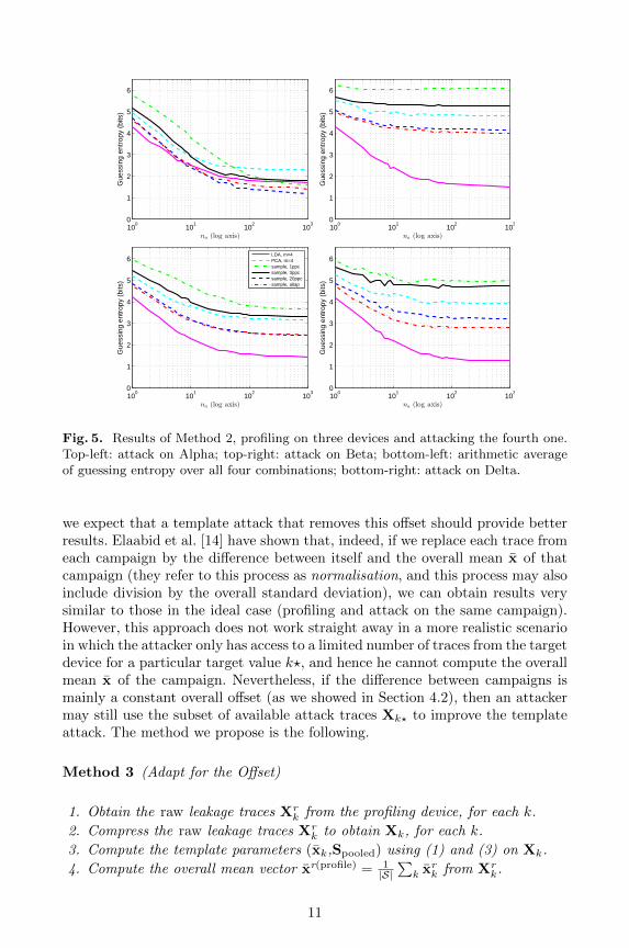
Fig. 5. Results of Method 2, profiling on three devices and attacking the fourth one.Top-left: attack on Alpha; top-right: attack on Beta; bottom-left: arithmetic averageof guessing entropy over all four combinations; bottom-right: attack on Delta.

we expect that a template attack that removes this offset should provide betterresults. Elaabid et al. [14] have shown that, indeed, if we replace each trace fromeach campaign by the difference between itself and the overall mean x of thatcampaign (they refer to this process as normalisation, and this process may alsoinclude division by the overall standard deviation), we can obtain results verysimilar to those in the ideal case (profiling and attack on the same campaign).However, this approach does not work straight away in a more realistic scenarioin which the attacker only has access to a limited number of traces from the targetdevice for a particular target value k?, and hence he cannot compute the overallmean x of the campaign. Nevertheless, if the difference between campaigns ismainly a constant overall offset (as we showed in Section 4.2), then an attackermay still use the subset of available attack traces Xk? to improve the templateattack. The method we propose is the following.

Method 3 (Adapt for the Offset)

1. Obtain the raw leakage traces Xrk from the profiling device, for each k.

2. Compress the raw leakage traces Xrk to obtain Xk, for each k.

3. Compute the template parameters (xk,Spooled) using (1) and (3) on Xk.

4. Compute the overall mean vector xr(profile) = 1|S|∑

k xrk from Xr

k.

11

5. Compute the constant offset c(profile) = offset(xr(profile)) ∈ R.5

6. Obtain the leakage traces Xk? from the attacked device.7. Compute the offset c(attack) = offset(xr) ∈ R from each raw attack trace xr

(row of Xrk?). As in step 5, for our data we used the median of xr.

8. Replace each trace xr (row of Xrk?) by xr(robust) = xr−1r·(c(attack)−c(profile)),

where 1r = [1, 1, . . . , 1] ∈ Rmr

.9. Apply the compression method to each of the modified attack traces xr(robust),

obtaining the robust attack leakage matrix X(robust)k? .

10. Compute the guessing entropy as described in Section 2.1 using X(robust)k? .

Note that instead of Method 3 we could also compensate for the offset (c(attack)−c(profile)) in the template parameters (xk,Spooled), but that would require muchmore computation, especially if we want to evaluate the expected success of anattacker using this method with an arbitrary number of attack traces, as wedo in this paper. Note also that in our evaluation, each additional attack traceimproves the offset difference estimation of the attacker: the use of the lineardiscriminant from (4) in our evaluation implies that, as we get more attacktraces, we are basically averaging the differences (c(attack)−c(profile)), thus gettinga better estimate of this difference.

In Figure 6 we show the results of Method 3. We can see that, on average, weget a similar pattern as with Method 2, but slightly worse results. For the bestcase (top-right), LDA is now achieving less than 1 bit of entropy at na = 1000,thus approaching the results on the ideal scenario. On the other hand, we alsosee that for the worst case (top-left) we get very bad results, where even usingLDA with na = 1000 doesn’t provide any real improvement. This large differencebetween the best and worst cases can be explained by looking at Figure 3. Therewe see that the difference between the overall means x of Alpha and Beta isconstant across the regions of high SNR (e.g. around samples 878 and 884),while the difference between Beta and Delta varies around these samples. Thissuggests that, in general, there is more than a simple DC offset involved betweendifferent campaigns and therefore this offset compensation method alone is notlikely to be helpful.

We could also try to use a high-pass filter, but note that a simple DC blockhas a non-local effect, i.e. a far-away bump in the trace not related to k can affectthe leakage samples that matter most. Another possibility, to deal with the low-frequency offset, might be to use electromagnetic leakage, as this leakage is notaffected by low-frequency components, so it may provide better results [16].

5.3 Profiling on Multiple Devices and Compensating for the Offset

If an attacker can use multiple devices during profiling, and since compensatingfor the offset may help where this offset is the main difference between campaigns,a possible option is to combine the previous methods. This leads to the following.

5 We used the median value of xr(profile) as the offset, since it provides a very goodapproximation with our data. However, when using a higher clock frequency, themedian can become very noisy, so we might have to find more robust methods.

12

100

101

102

103

0

1

2

3

4

5

6

na (log axis)

Gue

ssin

g en

trop

y (b

its)

100

101

102

103

0

1

2

3

4

5

6

na (log axis)

Gue

ssin

g en

trop

y (b

its)

100

101

102

103

0

1

2

3

4

5

6

na (log axis)

Gue

ssin

g en

trop

y (b

its)

LDA, m=4PCA, m=4sample, 1ppcsample, 3ppcsample, 20ppcsample, allap

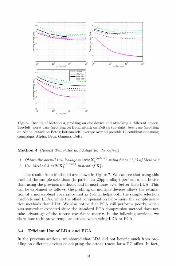
Fig. 6. Results of Method 3, profiling on one device and attacking a different device.Top-left: worst case (profiling on Beta, attack on Delta); top-right: best case (profilingon Alpha, attack on Beta); bottom-left: average over all possible 12 combinations usingcampaigns Alpha, Beta, Gamma, Delta.

Method 4 (Robust Templates and Adapt for the Offset)

1. Obtain the overall raw leakage matrix Xr(robust)k using Steps (1,2) of Method 2.

2. Use Method 3 with Xr(robust)k instead of Xr

k.

The results from Method 4 are shown in Figure 7. We can see that using thismethod the sample selections (in particular 20ppc, allap) perform much betterthan using the previous methods, and in most cases even better than LDA. Thiscan be explained as follows: the profiling on multiple devices allows the estima-tion of a more robust covariance matrix (which helps both the sample selectionmethods and LDA), while the offset compensation helps more the sample selec-tion methods than LDA. We also notice that PCA still performs poorly, whichwas somewhat expected since the standard PCA compression method does nottake advantage of the robust covariance matrix. In the following sections, weshow how to improve template attacks when using LDA or PCA.

5.4 Efficient Use of LDA and PCA

In the previous sections, we showed that LDA did not benefit much from pro-filing on different devices or adapting the attack traces for a DC offset. In fact,

13

100

101

102

103

0

1

2

3

4

5

6

na (log axis)

Gue

ssin

g en

trop

y (b

its)

100

101

102

103

0

1

2

3

4

5

6

na (log axis)

Gue

ssin

g en

trop

y (b

its)

100

101

102

103

0

1

2

3

4

5

6

na (log axis)

Gue

ssin

g en

trop

y (b

its)

LDA, m=4PCA, m=4sample, 1ppcsample, 3ppcsample, 20ppcsample, allap

100

101

102

103

0

1

2

3

4

5

6

na (log axis)

Gue

ssin

g en

trop

y (b

its)

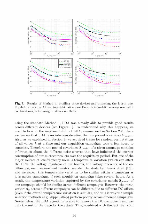
Fig. 7. Results of Method 4, profiling three devices and attacking the fourth one.Top-left: attack on Alpha; top-right: attack on Beta; bottom-left: average over all 4combinations; bottom-right: attack on Delta.

using the standard Method 1, LDA was already able to provide good resultsacross different devices (see Figure 1). To understand why this happens, weneed to look at the implementation of LDA, summarised in Section 2.2. Therewe can see that LDA takes into consideration the raw pooled covariance Spooled.Also, as we explained in Section 3, we acquired traces for random permutationsof all values k at a time and our acquisition campaigns took a few hours tocomplete. Therefore, the pooled covariance Spooled of a given campaign containsinformation about the different noise sources that have influenced the currentconsumption of our microcontrollers over the acquisition period. But one of themajor sources of low-frequency noise is temperature variation (which can affectthe CPU, the voltage regulator of our boards, the voltage reference of the os-cilloscope, our measurement resistor; see also the study by Heuser et al. [15]),and we expect this temperature variation to be similar within a campaign asit is across campaigns, if each acquisition campaign takes several hours. As aresult, the temperature variation captured by the covariance matrix Spooled ofone campaign should be similar across different campaigns. However, the meanvectors xk across different campaigns can be different due to different DC offsets(even if the overall temperature variation is similar), and this is why the sampleselection methods (e.g. 20ppc, allap) perform poorly across different campaigns.Nevertheless, the LDA algorithm is able to remove the DC component and useonly the rest of the trace for the attack. This, combined with the fact that with

14

0 5 10 15 20 25 30 35 40−0.5

0

0.5

1

1.5

2

0 5 10 15 20 25 30 35 40−10

0

10

20

30

40

50

0 5 10 15 20 25 30 35 40−10

0

10

20

30

40

50

0 500 1000 1500 2000 2500

u1u2u3u4u5u6

0 500 1000 1500 2000 2500

u1u2u3u4u5u6

0 500 1000 1500 2000 2500

u1u2u3u4u5u6

0 5 10 15 2010

3

104

105

106

107

0 5 10 15 2010

9

1010

1011

1012

1013

1014

LDA (S−1pooledB) PCA (B) Spooled

eigenvector index

sample index

DC

com

ponen

t

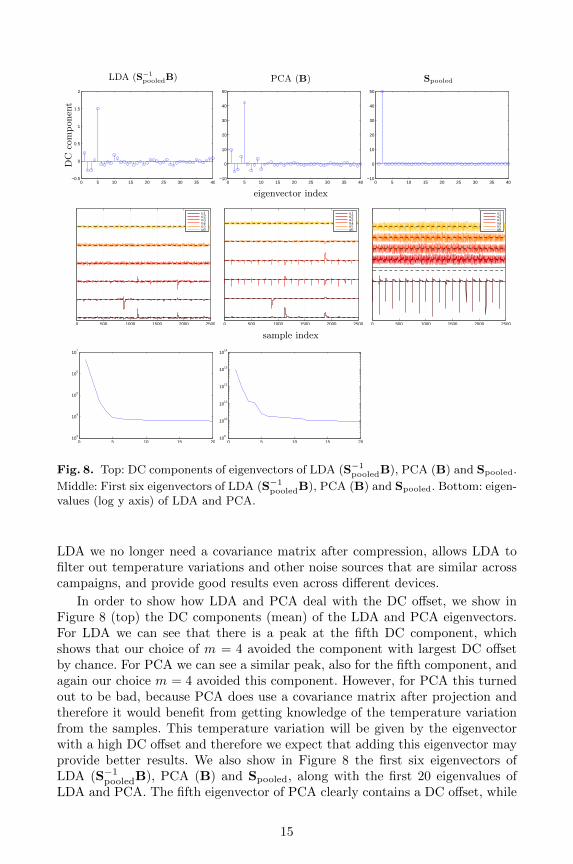
Fig. 8. Top: DC components of eigenvectors of LDA (S−1pooledB), PCA (B) and Spooled.

Middle: First six eigenvectors of LDA (S−1pooledB), PCA (B) and Spooled. Bottom: eigen-

values (log y axis) of LDA and PCA.

LDA we no longer need a covariance matrix after compression, allows LDA tofilter out temperature variations and other noise sources that are similar acrosscampaigns, and provide good results even across different devices.

In order to show how LDA and PCA deal with the DC offset, we show inFigure 8 (top) the DC components (mean) of the LDA and PCA eigenvectors.For LDA we can see that there is a peak at the fifth DC component, whichshows that our choice of m = 4 avoided the component with largest DC offsetby chance. For PCA we can see a similar peak, also for the fifth component, andagain our choice m = 4 avoided this component. However, for PCA this turnedout to be bad, because PCA does use a covariance matrix after projection andtherefore it would benefit from getting knowledge of the temperature variationfrom the samples. This temperature variation will be given by the eigenvectorwith a high DC offset and therefore we expect that adding this eigenvector mayprovide better results. We also show in Figure 8 the first six eigenvectors ofLDA (S−1

pooledB), PCA (B) and Spooled, along with the first 20 eigenvalues ofLDA and PCA. The fifth eigenvector of PCA clearly contains a DC offset, while

15

100

101

102

103

0

1

2

3

4

5

6

na (log axis)

Gue

ssin

g en

trop

y (b

its)

LDA, m=4PCA, m=4sample, 1ppcsample, 3ppcsample, 20ppcsample, allapLDA, m=3LDA, m=5LDA, m=6LDA, m=40PCA, m=5PCA, m=6PCA, m=40

100

101

102

103

0

1

2

3

4

5

6

na (log axis)

Gue

ssin

g en

trop

y (b

its)

LDA, m=4LDA, m=5PCA, m=4PCA, m=5

LDA m = 3,m = 4

PCA m = 4

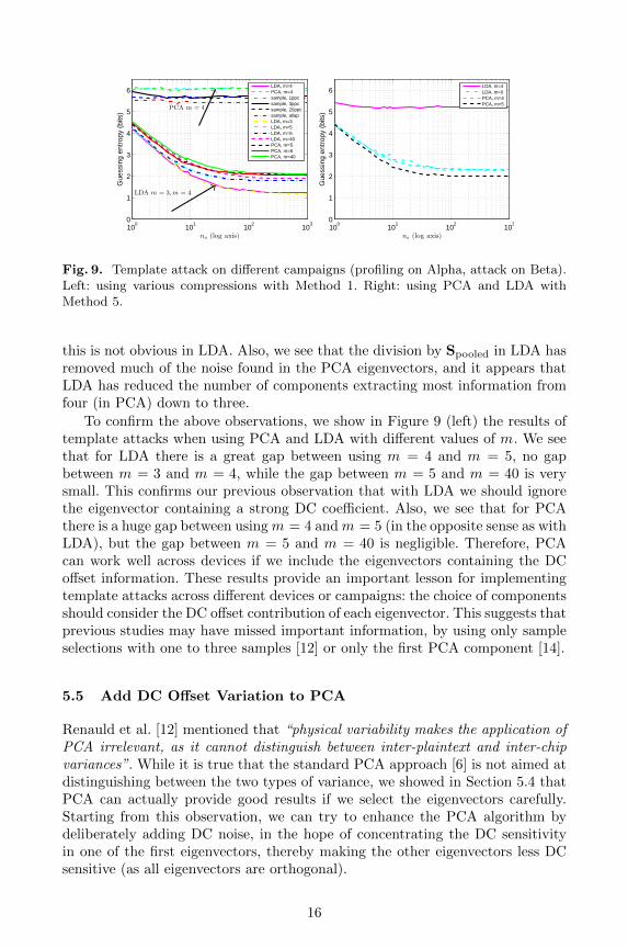
Fig. 9. Template attack on different campaigns (profiling on Alpha, attack on Beta).Left: using various compressions with Method 1. Right: using PCA and LDA withMethod 5.

this is not obvious in LDA. Also, we see that the division by Spooled in LDA hasremoved much of the noise found in the PCA eigenvectors, and it appears thatLDA has reduced the number of components extracting most information fromfour (in PCA) down to three.

To confirm the above observations, we show in Figure 9 (left) the results oftemplate attacks when using PCA and LDA with different values of m. We seethat for LDA there is a great gap between using m = 4 and m = 5, no gapbetween m = 3 and m = 4, while the gap between m = 5 and m = 40 is verysmall. This confirms our previous observation that with LDA we should ignorethe eigenvector containing a strong DC coefficient. Also, we see that for PCAthere is a huge gap between usingm = 4 andm = 5 (in the opposite sense as withLDA), but the gap between m = 5 and m = 40 is negligible. Therefore, PCAcan work well across devices if we include the eigenvectors containing the DCoffset information. These results provide an important lesson for implementingtemplate attacks across different devices or campaigns: the choice of componentsshould consider the DC offset contribution of each eigenvector. This suggests thatprevious studies may have missed important information, by using only sampleselections with one to three samples [12] or only the first PCA component [14].

5.5 Add DC Offset Variation to PCA

Renauld et al. [12] mentioned that “physical variability makes the application ofPCA irrelevant, as it cannot distinguish between inter-plaintext and inter-chipvariances”. While it is true that the standard PCA approach [6] is not aimed atdistinguishing between the two types of variance, we showed in Section 5.4 thatPCA can actually provide good results if we select the eigenvectors carefully.Starting from this observation, we can try to enhance the PCA algorithm bydeliberately adding DC noise, in the hope of concentrating the DC sensitivityin one of the first eigenvectors, thereby making the other eigenvectors less DCsensitive (as all eigenvectors are orthogonal).

16

0 5 10 15 20 25 30 35 40−35

−30

−25

−20

−15

−10

−5

0

5

0 5 10 15 20 25 30 35 40−50

−40

−30

−20

−10

0

10

0 500 1000 1500 2000 2500

u1u2u3u4u5u6

0 500 1000 1500 2000 2500

u1u2u3u4u5u6

LDA (S−1pooledB) PCA (B)

eigenvector index

sample index

DC

com

ponen

t

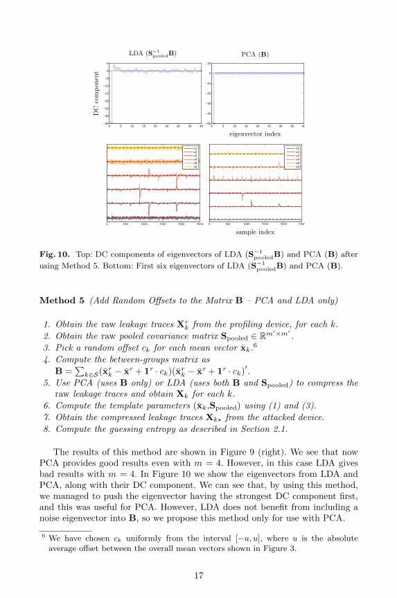
Fig. 10. Top: DC components of eigenvectors of LDA (S−1pooledB) and PCA (B) after

using Method 5. Bottom: First six eigenvectors of LDA (S−1pooledB) and PCA (B).

Method 5 (Add Random Offsets to the Matrix B – PCA and LDA only)

1. Obtain the raw leakage traces Xrk from the profiling device, for each k.

2. Obtain the raw pooled covariance matrix Spooled ∈ Rmr×mr

.

3. Pick a random offset ck for each mean vector xk.6

4. Compute the between-groups matrix as

B =∑

k∈S(xrk − xr + 1r · ck)(xr

k − xr + 1r · ck)′.

5. Use PCA (uses B only) or LDA (uses both B and Spooled) to compress theraw leakage traces and obtain Xk for each k.

6. Compute the template parameters (xk,Spooled) using (1) and (3).

7. Obtain the compressed leakage traces Xk? from the attacked device.

8. Compute the guessing entropy as described in Section 2.1.

The results of this method are shown in Figure 9 (right). We see that nowPCA provides good results even with m = 4. However, in this case LDA givesbad results with m = 4. In Figure 10 we show the eigenvectors from LDA andPCA, along with their DC component. We can see that, by using this method,we managed to push the eigenvector having the strongest DC component first,and this was useful for PCA. However, LDA does not benefit from including anoise eigenvector into B, so we propose this method only for use with PCA.

6 We have chosen ck uniformly from the interval [−u, u], where u is the absoluteaverage offset between the overall mean vectors shown in Figure 3.

17

6 Conclusions

In this paper, we explored the efficacy of template attacks when using differentdevices for the profiling and attack steps.

We observed that, for our Atmel XMEGA 256 A3U 8-bit microcontrollerand particular setup, the campaign-dependent parameters (temperature, envi-ronmental noise, etc.) appear to be the dominant factors in differences betweencampaign data, not the inter-device variability. These differences rendered thestandard template attack useless for all common compression methods exceptFisher’s Linear Discriminant Analysis (LDA). To improve the performance ofthe attack across different devices, we explored several variants of the templateattack, that compensate for a DC offset in the attack phase, or profile acrossmultiple devices. By combining these options, we can improve the results of tem-plate attacks. However, these methods did not provide a great advantage whenusing Principal Component Analysis (PCA) or LDA.

Based on detailed analysis of LDA, we offered an explanation why this com-pression method works well across different devices: LDA is able to compensatetemperature variation captured by the pooled covariance matrix and this tem-perature variation is similar across campaigns. From this analysis, we were ableto provide guidance for an efficient use of both LDA and PCA across differentdevices or campaigns: for LDA we should ignore the eigenvectors starting withthe one having the strongest DC contribution, while for PCA we should chooseenough components to include at least the one with the strongest DC contri-bution. Based on these observations we also proposed a method to enhance thePCA algorithm such that the eigenvector with the strongest DC contributioncorresponds to the largest eigenvalue and this allows PCA to provide good re-sults across different devices even when using a small number of eigenvectors.

Our results show that the choice of compression method and parameters (e.g.choice of eigenvectors for PCA and LDA) has a strong impact on the successof template attacks across different devices, a fact that was not evidenced inprevious studies. As a guideline, when using sample selection we should use alarge number of samples, profile on multiple devices and adapt for a DC offset,but with LDA and PCA we may use the standard template attack and performthe profiling on a single device, if we select the eigenvectors according to theirDC component. Overall, LDA seems the best compression method when usingtemplate attacks across different devices, but it requires to invert a possibly largecovariance matrix, which might not be possible with a small number of profilingtraces. In such cases, PCA might be a better alternative.

We conclude that with a careful choice of compression method we can obtaintemplate attacks that are efficient also across different devices, reducing theguessing entropy of an unknown 8-bit value below 1.5 bits.

Data and Code Availability: In the interest of reproducible research we makeavailable our data and related MATLAB scripts at:

http://www.cl.cam.ac.uk/research/security/datasets/grizzly/

18

Acknowledgement: Omar Choudary is a recipient of the Google Europe Fellowship in

Mobile Security, and this research is supported in part by this Google Fellowship. The

opinions expressed in this paper do not represent the views of Google unless otherwise

explicitly stated.

References

1. P. Kocher, J. Jaffe, and B. Jun, “Differential Power Analysis”, CRYPTO 1999,LNCS 1666, pp 388–397.

2. S. Chari, J. Rao, and P. Rohatgi, “Template Attacks”, in CHES 2002, LNCS2523, pp 13–28.

3. E. Brier, C. Clavier, and F. Olivier, “Correlation Power Analysis with a LeakageModel”, in CHES 2004, LNCS 3156, pp 16–29.

4. W. Schindler, K. Lemke, and C. Paar, “A Stochastic Model for Differential SideChannel Cryptanalysis”, in CHES 2005, LNCS 3659, pp 30–46.

5. B. Gierlichs, K. Lemke-Rust, and C. Paar, “Templates vs. Stochastic Methods”,in CHES 2006, LNCS 4249, 2006, pp 15–29.

6. C. Archambeau, E. Peeters, F. Standaert, and J. Quisquater, “Template Attacksin Principal Subspaces”, in CHES 2006, LNCS 4249, 2006, pp 1–14.

7. N. Homma, S. Nagashima, Y. Imai, T. Aoki, and A. Satoh, “High-ResolutionSide-Channel Attack Using Phase-Based Waveform Matching”, in CHES 2006,LNCS 4249, 2006, pp 187–200.

8. F.-X. Standaert and C. Archambeau, “Using Subspace-Based Template Attacksto Compare and Combine Power and Electromagnetic Information Leakages”,in CHES 2008, LNCS 5154, pp 411–425.

9. B. Gierlichs, L. Batina, P. Tuyls, and B. Preneel, “Mutual Information Analy-sis”, in CHES 2008, LNCS 5154, pp 426–442.

10. F.-X. Standaert, T. G. Malkin, and M. Yung, “A Unified Framework for theAnalysis of Side-Channel Key Recovery Attacks”, EUROCRYPT 2009, LNCS5479, pp 443–461.

11. F.-X. Standaert, F. Koeune, and W. Schindler, “How to Compare Profiled Side-Channel Attacks?” in Applied Cryptography and Network Security, LNCS 5536,pp 485–498.

12. M. Renauld, F.-X. Standaert, N. Veyrat-Charvillon, D. Kamel, and D. Flan-dre, “A Formal Study of Power Variability Issues and Side-Channel Attacks forNanoscale Devices”, in EUROCRYPT 2011, LNCS 6632, pp 109–128.

13. D. Oswald and C. Paar, “Breaking Mifare DESFire MF3ICD40: Power Analysisand Templates in the Real World”, in CHES 2011, LNCS 6917, pp 207–222.

14. M. A. Elaabid and S. Guilley, “Portability of templates”, Journal of Crypto-graphic Engineering, 2(1), pp 63–74, 2012.

15. A. Heuser, M. Kasper, W. Schindler, and M. Stottinger, “A New DifferenceMethod for Side-Channel Analysis with High-Dimensional Leakage Models”, inCT-RSA 2012, LNCS 7178, pp. 365–382.

16. V. Lomne, E. Prouff, and T. Roche, “Behind the Scene of Side Channel Attacks”,in ASIACRYPT 2013, Part I, LNCS 8269, pp. 506–525.

17. O. Choudary and M. G. Kuhn, “Efficient Template Attacks”, in CARDIS 2013,LNCS 8419, pp. 253–270.

19