SANDIA REPORT SAND2012-1366 Unlimited Release Printed February 22, 2012
Technical Analysis of Prospective Photovoltaic Systems in Utah
Jimmy E. Quiroz and Christopher P. Cameron
Prepared by Sandia National Laboratories Albuquerque, New Mexico 87185 and Livermore, California 94550
Sandia National Laboratories is a multi-program laboratory managed and operated by Sandia Corporation, a wholly owned subsidiary of Lockheed Martin Corporation, for the U.S. Department of Energy’s National Nuclear Security Administration under Contract DE-AC04-94AL85000.
Approved for public release; further dissemination unlimited.

2
Issued by Sandia National Laboratories, operated for the United States Department of Energy
by Sandia Corporation.
NOTICE: This report was prepared as an account of work sponsored by an agency of the
United States Government. Neither the United States Government, nor any agency thereof,
nor any of their employees, nor any of their contractors, subcontractors, or their employees,
make any warranty, express or implied, or assume any legal liability or responsibility for the
accuracy, completeness, or usefulness of any information, apparatus, product, or process
disclosed, or represent that its use would not infringe privately owned rights. Reference herein
to any specific commercial product, process, or service by trade name, trademark,
manufacturer, or otherwise, does not necessarily constitute or imply its endorsement,
recommendation, or favoring by the United States Government, any agency thereof, or any of
their contractors or subcontractors. The views and opinions expressed herein do not
necessarily state or reflect those of the United States Government, any agency thereof, or any
of their contractors.
Printed in the United States of America. This report has been reproduced directly from the best
available copy.
Available to DOE and DOE contractors from
U.S. Department of Energy
Office of Scientific and Technical Information
P.O. Box 62
Oak Ridge, TN 37831
Telephone: (865) 576-8401
Facsimile: (865) 576-5728
E-Mail: [email protected]
Online ordering: http://www.osti.gov/bridge
Available to the public from
U.S. Department of Commerce
National Technical Information Service
5285 Port Royal Rd.
Springfield, VA 22161
Telephone: (800) 553-6847
Facsimile: (703) 605-6900
E-Mail: [email protected]
Online order: http://www.ntis.gov/help/ordermethods.asp?loc=7-4-0#online
3
SAND2012-1366
Unlimited Release
Printed February 22, 2012
Technical Analysis of Prospective Photovoltaic Systems in Utah
Jimmy E. Quiroz and Christopher P. Cameron
Photovoltaics and Distributed Systems Integration
Sandia National Laboratories
P.O. Box 5800
Albuquerque, New Mexico 87185-1033
Abstract
This report explores the technical feasibility of prospective utility-scale photovoltaic
system (PV) deployments in Utah. Sandia National Laboratories worked with Rocky
Mountain Power (RMP), a division of PacifiCorp operating in Utah, to evaluate
prospective 2-megawatt (MW) PV plants in different locations with respect to energy
production and possible impact on the RMP system and customers. The study focused
on 2-MWAC nameplate PV systems of different PV technologies and different
tracking configurations. Technical feasibility was evaluated at three different
potential locations in the RMP distribution system. An advanced distribution
simulation tool was used to conduct detailed time-series analysis on each feeder and
provide results on the impacts on voltage, demand, voltage regulation equipment
operations, and flicker. Annual energy performance was estimated.
4
ACKNOWLEDGMENTS
Abraham Ellis – Sandia National Laboratories – Principal Investigator
Thomas E. McDermott – MelTran, Inc. – OpenDSS File Conversions
Matthew Lave – Sandia National Laboratories – Electrical Analysis
Matthew J. Reno – Sandia National Laboratories – Electrical Analysis
Geoffrey Taylor Klise – Sandia National Laboratories – PVsyst Analysis
Jim Lacey – PacifiCorp Energy/Rocky Mountain Power – Project Support
Nathan Wilson – PacifiCorp Energy/Rocky Mountain Power – Distribution System Support
Gregory Bean – PacifiCorp Energy/Rocky Mountain Power – Distribution System Support
Luke Hoffman - PacifiCorp Energy/Rocky Mountain Power – Distribution System Support

5
CONTENTS
EXECUTIVE SUMMARY ............................................................................................................ 9
1 INTRODUCTION ................................................................................................................. 11 1.1 Overview ...................................................................................................................... 11 1.2 Electrical Performance Analysis .................................................................................. 11
1.2.1 Feeder Modeling ............................................................................................... 13 1.2.2 Selection of Study Periods ............................................................................... 13 1.2.3 Time Series Data Inputs ................................................................................... 15
1.3 Performance Analysis ................................................................................................... 16
2 ELECTRICAL PERFORMANCE ANALYSIS ................................................................... 17
2.1 Toquerville 11 .............................................................................................................. 17
2.1.1 Peak PV Penetration Period ............................................................................. 19
2.1.2 Peak Load Period .............................................................................................. 24 2.1.3 Toquerville 11 Summary .................................................................................. 28
2.2 Delta 11 ........................................................................................................................ 28 2.2.1 Peak PV Penetration Period ............................................................................. 30
2.2.2 Peak Load Period .............................................................................................. 34 2.2.3 Delta 11 Summary ............................................................................................ 39
2.3 Terminal 19 .................................................................................................................. 40
2.3.1 Peak PV Penetration Load Period .................................................................... 42 2.3.2 Peak Load Period .............................................................................................. 46
2.3.3 Terminal 19 Summary ...................................................................................... 51
3 PERFORMANCE MODELING ........................................................................................... 52
3.1 Solar System Designs ................................................................................................... 52 3.2 Analytical Approach ..................................................................................................... 58
3.2.1 Performance Analysis ....................................................................................... 58 3.3 Results .......................................................................................................................... 58
4 CONCLUSION ..................................................................................................................... 64
6
FIGURES
Figure 1. IEEE Std 141-1993 voltage flicker limits [4]. ...............................................................12 Figure 2. Feeder source impedance modeling. .............................................................................13 Figure 3. Toquerville 11 peak PV penetration period load shape.................................................14 Figure 4. PV output profile (one day). ..........................................................................................15
Figure 5. Toquerville Feeder 11 PV plant location.......................................................................17 Figure 6. Toquerville Feeder 11....................................................................................................18 Figure 7. Toquerville 11 2010 average load amps. .......................................................................19 Figure 8. Toquerville Peak PV Penetration period maximum voltage profiles – with and
without PV. ..............................................................................................................................20
Figure 9. Toquerville Peak PV Penetration period minimum voltage profiles – with and
without PV. ..............................................................................................................................20
Figure 10. Toquerville 11 net power without PV during Peak PV Penetration period. ...............22 Figure 11. Toquerville 11 peak PV Penetration period net power with PV. ................................23 Figure 12. Toquerville peak period maximum voltage profiles – with and without PV. .............24 Figure 13. Toquerville peak period minimum voltage profiles – with and without PV. ..............25
Figure 14. Toquerville 11 peak period net power without PV. ....................................................26 Figure 15. Toquerville 11 peak period net power with PV...........................................................27 Figure 16. Delta Feeder 11 PV plant location...............................................................................28
Figure 17. Delta Feeder 11............................................................................................................29 Figure 18. Delta 11 2010 average load amps. ...............................................................................30
Figure 19. Delta peak PV Penetration period maximum voltage profiles – with and without
PV. ...........................................................................................................................................31 Figure 20. Delta peak PV Penetration period minimum voltage profiles – with and without
PV. ...........................................................................................................................................31
Figure 21. Delta 11 Peak PV Penetration period net power without PV. .....................................33 Figure 22. Delta 11 Peak PV Penetration period net power with PV. ..........................................34 Figure 23. Delta peak period maximum voltage profiles – with and without PV. .......................35
Figure 24. Delta peak period minimum voltage profiles – with and without PV. ........................35 Figure 25. Delta 11 peak period net power without PV. ..............................................................37
Figure 26. Delta 11 peak period net power with PV. ....................................................................38 Figure 27. Terminal Feeder 19 PV plant location.........................................................................40 Figure 28. Terminal Feeder 19......................................................................................................41 Figure 29. Terminal 19 2009 average load amps. .........................................................................42
Figure 30. Terminal peak PV penetration period maximum voltage profiles – with and
without PV. ..............................................................................................................................43 Figure 31. Terminal peak PV penetration period minimum voltage profiles – with and
without PV. ..............................................................................................................................43 Figure 32. Terminal 19 Peak PV Penetration period net power without PV. ...............................45 Figure 33. Terminal 19 Peak PV Penetration period net power with PV. ....................................46 Figure 34. Terminal peak period maximum voltage profiles – with and without PV. .................47
Figure 35. Terminal peak period minimum voltage profiles – with and without PV. ..................47 Figure 36. Terminal 19 peak period net power without PV. ........................................................49 Figure 37. Terminal 19 peak period net power with PV...............................................................50
Figure 38. Fixed-tilt multicrystalline system. ...............................................................................54
7
Figure 39. Fixed-tilt thin-film system. ..........................................................................................55
Figure 40. Single-axis tracking multicrystalline system. ..............................................................56 Figure 41. Toquerville: system output by month. .........................................................................59 Figure 42. Delta: system output by month. ...................................................................................60
Figure 43. Terminal: system output by month. .............................................................................60 Figure 44. Toquerville: average hourly output by month. ............................................................61 Figure 45. Delta: average hourly output by month. ......................................................................62 Figure 46. Terminal: average hourly output by month. ................................................................63
TABLES
Table ES-1. Toquerville 11 Results Summary. ............................................................................10
Table ES-2. Performance Results Summary. ................................................................................10 Table 1. ANSI C84.1 Range A and B Service Voltage Limits (120- and 7200-V Bases) [3]. ....12 Table 2. Study Periods. .................................................................................................................14 Table 3. Toquerville Peak PV Penetration Period Maximum and Minimum Voltages – 120-
V Base. .....................................................................................................................................21 Table 4. Toquerville Peak Period Maximum and Minimum Voltages – 120-V Base. ................25 Table 5. Toquerville 11 Results Summary. ..................................................................................28
Table 6. Delta Peak PV Penetration Period Maximum and Minimum Voltages – 120-V
Base. .........................................................................................................................................32
Table 7. Delta Peak Period Maximum and Minimum Voltages – 120-V Base. ..........................36 Table 8. Delta 11 Results Summary. ............................................................................................39 Table 9. Terminal Peak PV Penetration Period Maximum and Minimum Voltages – 120-V
Base. .........................................................................................................................................44
Table 10. Terminal Peak Period Maximum and Minimum Voltages – 120-V Base. ..................48 Table 11. Terminal 19 Results Summary. ....................................................................................51 Table 12. System Designs. ............................................................................................................53
Table 13. Summary of Energy Output ..........................................................................................59

8
9
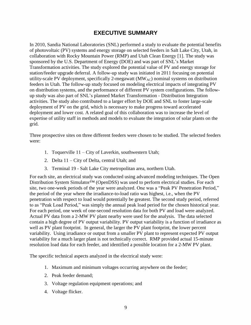
EXECUTIVE SUMMARY
In 2010, Sandia National Laboratories (SNL) performed a study to evaluate the potential benefits
of photovoltaic (PV) systems and energy storage on selected feeders in Salt Lake City, Utah, in
collaboration with Rocky Mountain Power (RMP) and Utah Clean Energy [1]. The study was
sponsored by the U.S. Department of Energy (DOE) and was part of SNL’s Market
Transformation activities. The study explored the potential value of PV and energy storage for
station/feeder upgrade deferral. A follow-up study was initiated in 2011 focusing on potential
utility-scale PV deployment, specifically 2-megawatt (MWAC) nominal systems on distribution
feeders in Utah. The follow-up study focused on modeling electrical impacts of integrating PV
on distribution systems, and the performance of different PV system configurations. The follow-
up study was also part of SNL’s planned Market Transformation - Distribution Integration
activities. The study also contributed to a larger effort by DOE and SNL to foster large-scale
deployment of PV on the grid, which is necessary to make progress toward accelerated
deployment and lower cost. A related goal of this collaboration was to increase the level of
expertise of utility staff in methods and models to evaluate the integration of solar plants on the
grid.
Three prospective sites on three different feeders were chosen to be studied. The selected feeders
were:
1. Toquerville 11 – City of Laverkin, southwestern Utah;
2. Delta 11 – City of Delta, central Utah; and
3. Terminal 19 - Salt Lake City metropolitan area, northern Utah.
For each site, an electrical study was conducted using advanced modeling techniques. The Open
Distribution System Simulator™ (OpenDSS) was used to perform electrical studies. For each
site, two one-week periods of the year were analyzed. One was a “Peak PV Penetration Period,”
the period of the year where the irradiance-to-load ratio was highest, i.e., when the PV
penetration with respect to load would potentially be greatest. The second study period, referred
to as “Peak Load Period,” was simply the annual peak load period for the chosen historical year.
For each period, one week of one-second resolution data for both PV and load were analyzed.
Actual PV data from a 2-MW PV plant nearby were used for the analysis. The data selected
contain a high degree of PV output variability. PV output variability is a function of irradiance as
well as PV plant footprint. In general, the larger the PV plant footprint, the lower percent
variability. Using irradiance or output from a smaller PV plant to represent expected PV output
variability for a much larger plant is not technically correct. RMP provided actual 15-minute
resolution load data for each feeder, and identified a possible location for a 2-MW PV plant.
The specific technical aspects analyzed in the electrical study were:
1. Maximum and minimum voltages occurring anywhere on the feeder;
2. Peak feeder demand;
3. Voltage regulation equipment operations; and
4. Voltage flicker.
10
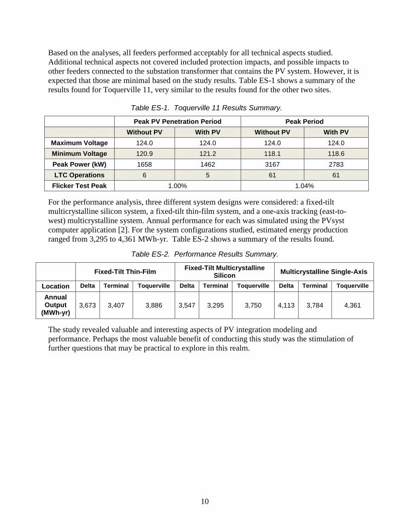
Based on the analyses, all feeders performed acceptably for all technical aspects studied.
Additional technical aspects not covered included protection impacts, and possible impacts to
other feeders connected to the substation transformer that contains the PV system. However, it is
expected that those are minimal based on the study results. Table ES-1 shows a summary of the
results found for Toquerville 11, very similar to the results found for the other two sites.
Table ES-1. Toquerville 11 Results Summary.
Peak PV Penetration Period Peak Period
Without PV With PV Without PV With PV
Maximum Voltage 124.0 124.0 124.0 124.0
Minimum Voltage 120.9 121.2 118.1 118.6
Peak Power (kW) 1658 1462 3167 2783
LTC Operations 6 5 61 61
Flicker Test Peak 1.00% 1.04%
For the performance analysis, three different system designs were considered: a fixed-tilt
multicrystalline silicon system, a fixed-tilt thin-film system, and a one-axis tracking (east-to-
west) multicrystalline system. Annual performance for each was simulated using the PVsyst
computer application [2]. For the system configurations studied, estimated energy production
ranged from 3,295 to 4,361 MWh-yr. Table ES-2 shows a summary of the results found.
Table ES-2. Performance Results Summary.
Fixed-Tilt Thin-Film Fixed-Tilt Multicrystalline
Silicon Multicrystalline Single-Axis
Location Delta Terminal Toquerville Delta Terminal Toquerville Delta Terminal Toquerville
Annual Output
(MWh-yr) 3,673 3,407 3,886 3,547 3,295 3,750 4,113 3,784 4,361
The study revealed valuable and interesting aspects of PV integration modeling and
performance. Perhaps the most valuable benefit of conducting this study was the stimulation of
further questions that may be practical to explore in this realm.
11
1 INTRODUCTION
1.1 Overview
This study focuses on two aspects of photovoltaic (PV) integration: modeling and analysis of
electrical impacts on distribution feeders, and performance analysis of three different PV
configurations. Three prospective locations on distribution feeders in Utah were chosen to be
studied for integration of 2-megawatt (MW) nominal PV systems:
1. Toquerville 11 (37.25 N, -113.25 W) – City of Laverkin, southwestern Utah;
2. Delta 11 (39.35 N, -112.55 W) – City of Delta, central Utah; and
3. Terminal 19 (40.75 N, - 112.05 W) – Salt Lake City metropolitan area, northern Utah.
For each location, three PV system configurations were evaluated: fixed mounting with both
multicrystalline silicon and thin-film, and single axis tracking with multicrystalline silicon.
Results of the study are presented in this report. Section 2 discusses representation of solar
output and electrical modeling of distribution circuits. Analysis results are discussed for each
case. Section 3 covers performance analysis and PV system design. A summary of assumptions
and technical approach for electrical performance and performance analyses is provided below.
1.2 Electrical Performance Analysis
For each feeder, Rocky Mountain Power (RMP) and Sandia National Laboratories (SNL)
identified approximately 20 acres of land for use in developing site-specific solar data and
studying the impact on the local distribution system. SNL modeled the distribution system based
on data RMP provided, including feeder and substation data (impedances, thermal ratings, etc.),
and load distribution, with the objective of determining the impacts of connecting 2 MW of PV
at the selected locations. For the electrical study, each site was connected using a three-phase
line extension from existing nearby feeder backbone. Performance metrics studied included
maximum and minimum voltages occurring anywhere on the feeder, peak feeder demand,
voltage regulation equipment operations, and voltage flicker. Voltage ranges set forth by the
ANSI C84.1 [3] standard were used as guidelines for acceptable voltage levels. The ANSI
voltage ranges shown in Table 1 are for service voltage, which is defined as the point of common
coupling between customer and utility. All feeders were modeled down to the distribution
transformer primary, with loads defined on the system primary with associated transformer
rating. All resultant voltages referenced the primary system; voltage drop from primary to
customer point of common coupling would need to be considered beyond these values.
12
Table 1. ANSI C84.1 Range A and B Service Voltage Limits (120- and 7200-V Bases) [3].
Range A (V) Range B (V)
Upper Limit 126 (7560) 127 (7620)
Lower Limit 114 (6840) 110 (6600)
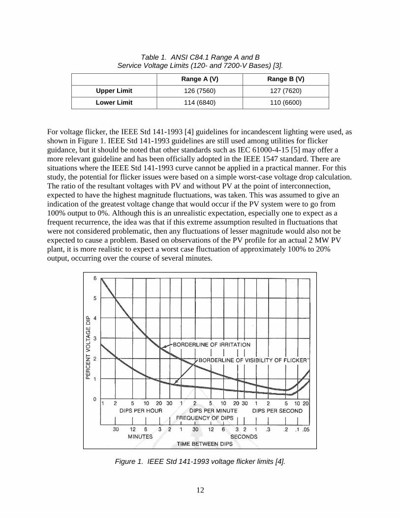
For voltage flicker, the IEEE Std 141-1993 [4] guidelines for incandescent lighting were used, as
shown in Figure 1. IEEE Std 141-1993 guidelines are still used among utilities for flicker
guidance, but it should be noted that other standards such as IEC 61000-4-15 [5] may offer a
more relevant guideline and has been officially adopted in the IEEE 1547 standard. There are
situations where the IEEE Std 141-1993 curve cannot be applied in a practical manner. For this
study, the potential for flicker issues were based on a simple worst-case voltage drop calculation.
The ratio of the resultant voltages with PV and without PV at the point of interconnection,
expected to have the highest magnitude fluctuations, was taken. This was assumed to give an
indication of the greatest voltage change that would occur if the PV system were to go from
100% output to 0%. Although this is an unrealistic expectation, especially one to expect as a
frequent recurrence, the idea was that if this extreme assumption resulted in fluctuations that
were not considered problematic, then any fluctuations of lesser magnitude would also not be
expected to cause a problem. Based on observations of the PV profile for an actual 2 MW PV
plant, it is more realistic to expect a worst case fluctuation of approximately 100% to 20%
output, occurring over the course of several minutes.
Figure 1. IEEE Std 141-1993 voltage flicker limits [4].
13
1.2.1 Feeder Modeling
For the electrical portion of the study, the OpenDSS simulation program was used. This open-
source platform is distributed by the Electric Power Research Institute (EPRI). One of the main
reasons for using OpenDSS, as opposed to industry-standard distribution analysis software (such
as ABB’s FeederAll used by RMP), was the ability to conduct high-resolution time series
studies. Planning studies using utility-standard simulation tools are not generally well suited for
sequential or dynamic simulations needed to fully characterize the effect of PV output variability
on distribution feeders.
To conduct the studies, feeder and load data were converted to OpenDSS format. The
conversion process consisted of extracting from FeederAll’s Microsoft® Access database format,
using primarily a custom Visual Basic script, developing a working case in OpenDSS format,
and validating the OpenDSS model by comparing power flow results to the FeederAll power
flow reports using the same load conditions. For example, voltage levels at each of the nodes of
the Terminal 19 feeder obtained with OpenDSS and FeederAll were compared for the peak load
condition. The largest voltage magnitude discrepancy observed was 1.76%, with the typical
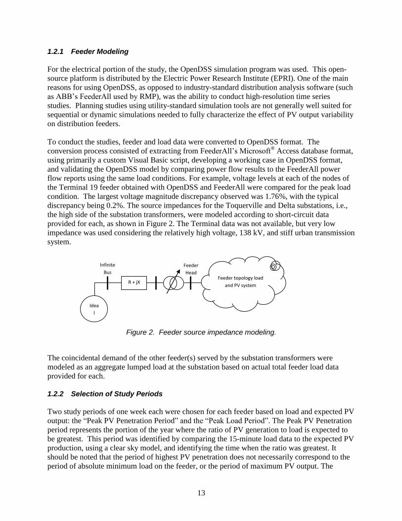
discrepancy being 0.2%. The source impedances for the Toquerville and Delta substations, i.e.,
the high side of the substation transformers, were modeled according to short-circuit data
provided for each, as shown in Figure 2. The Terminal data was not available, but very low
impedance was used considering the relatively high voltage, 138 kV, and stiff urban transmission
system.
Figure 2. Feeder source impedance modeling.
The coincidental demand of the other feeder(s) served by the substation transformers were
modeled as an aggregate lumped load at the substation based on actual total feeder load data
provided for each.
1.2.2 Selection of Study Periods
Two study periods of one week each were chosen for each feeder based on load and expected PV
output: the “Peak PV Penetration Period” and the “Peak Load Period”. The Peak PV Penetration
period represents the portion of the year where the ratio of PV generation to load is expected to
be greatest. This period was identified by comparing the 15-minute load data to the expected PV
production, using a clear sky model, and identifying the time when the ratio was greatest. It
should be noted that the period of highest PV penetration does not necessarily correspond to the
period of absolute minimum load on the feeder, or the period of maximum PV output. The
Idea
l
Gen
R + jX
Infinite
Bus
Feeder
Head
Feeder topology load
and PV system

14
second period, or “Peak Load Period,” was simply chosen based on the peak load for the year.
Table 2 lists the study periods chosen.
Table 2. Study Periods.
Site Peak PV Penetration Period (MST) Peak Load Period (MST)
Toquerville 11 Sunday, May 23, 2010 @ 12:00 PM Monday, July 19, 2010 @ 05:30 PM
Delta 11 Sunday, June 13, 2010 @ 12:45 PM Monday, August 2, 2010 @ 04:45 PM
Terminal 19 Sunday, June 7, 2009 @ 12:00 PM Thursday, August 13, 2009 @ 01:15 PM
For the purpose of incorporating day-of-the-week diversity, one full week surrounding the Peak
PV Penetration Period and Peak Load Period was used to assess feeder performance. Figure 3
shows the Toquerville 11 15-minute, three-phase average load shape for the Peak PV Penetration
period (kVA). The load level was calculated from the per-phase amps provided by RMP,
assuming 123 V on a 120-V base. The voltage assumption in this figure was made since only
load amps were provided. As can be seen in Figure 3, there is a significant difference between
Sunday and Thursday or Friday, thus justifying the value of studying the entire week.
Figure 3. Toquerville 11 peak PV penetration period load shape.
15
1.2.3 Time Series Data Inputs
1.2.3.1 PV System Data
The effect of PV output variability on grid voltage is often a concern during PV interconnection
studies. For the simulations in OpenDSS there were two basic time-series inputs used: PV
system output and load data. For the PV system outputs, actual data from an actual 2-MW, 20°
tilted single-axis tracking system operating in an area of similar weather characteristics were
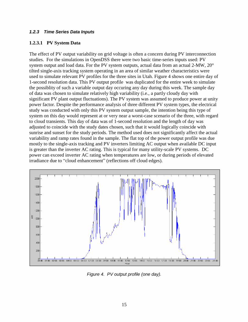
used to simulate relevant PV profiles for the three sites in Utah. Figure 4 shows one entire day of
1-second resolution data. This PV output profile was duplicated for the entire week to simulate
the possiblity of such a variable output day occuring any day during this week. The sample day
of data was chosen to simulate relatively high variability (i.e., a partly cloudy day with
significant PV plant output fluctuations). The PV system was assumed to produce power at unity
power factor. Despite the performance analysis of three different PV system types, the electrical
study was conducted with only this PV system output sample, the intention being this type of
system on this day would represent at or very near a worst-case scenario of the three, with regard
to cloud transients. This day of data was of 1-second resolution and the length of day was
adjusted to coincide with the study dates chosen, such that it would logically coincide with
sunrise and sunset for the study periods. The method used does not significantly affect the actual
variability and ramp rates found in the sample. The flat top of the power output profile was due
mostly to the single-axis tracking and PV inverters limiting AC output when available DC input
is greater than the inverter AC rating. This is typical for many utility-scale PV systems. DC
power can exceed inverter AC rating when temperatures are low, or during periods of elevated
irradiance due to “cloud enhancement” (reflections off cloud edges).
Figure 4. PV output profile (one day).

16
1.2.3.2 Load Data
One-second resolution load data files were created by interpolating the actual 15-minute
resolution data for the feeders. Balanced load conditions were assumed based on the actual data
three-phase average. An alternative to this may have been to insert some level of noise to
simulate variability; however, information necessary to estimate this was not available. The
amount of short-term variability introduced by a 2-MW PV system is expected to be far greater
than the variability associated with load aggregated at the feeder head; therefore, adding “noise”
to the 15-minute load data was not deemed necessary for this study. The feeder load was
allocated to each distribution transformer modeled along the entire feeder based on connected
kVA transformer sizes. A power factor of 0.9 lagging was assumed for each load. The presence
of PV will not change the reactive power demand, but it does affect the power factor as measured
at the feeder level. This is because of the reduction of real power, being supplied by the PV
system, while reactive power demand remains the same, thus reducing the ratio of real-to-
reactive power and making the power factor seem worse. This is important if any operations
depend on power factor thresholds at the feeder level.
System protection impacts were not analyzed in this study. Also, thermal overloads were not
identified in any of the cases. It was assumed that interconnection facilities were sized
appropriately for a PV output at 2 MW.
1.3 Performance Analysis
SNL also estimated the expected performance of the planned PV facilities. Three different
system designs were analyzed: a fixed-tilt multicrystalline silicon system, a fixed-tilt thin-film
system, and a one-axis tracking (east-to-west) multicrystalline system. Mechanical and electrical
designs for each of these three system configurations are presented in Section 3.
Annual performance for each was simulated using the PVsyst program. PVsyst was selected
because of its ability to model shading and tracking in large systems. For the fixed-tilt arrays,
shading was analyzed using the unlimited shed row option, which simplifies analysis by ignoring
the fact that the far east end of the rows are not shaded in the morning and the far west ends are
not shaded in the afternoon. Tracking limits of ±45° with backtracking were used for the one-
axis tracking array. The TMY-2 weather data were obtained from the Solar Prospector site [6].
Results of the performance analyses are shown in Section 3.

17
2 ELECTRICAL PERFORMANCE ANALYSIS
This section contains results of electrical performance analysis for each of the three feeders,
based on simulations.
2.1 Toquerville 11
Toquerville Substation is located in Toquerville, a small rural city near the southwestern corner
of Utah. The chosen PV site is approximately 0.7 miles east of Laverkin, as shown in Figure 5.
Electrically, the PV point of interconnection is approximately 1.3 miles from Toquerville
Substation. A nominal 2-MW PV system represents approximately 63% of peak load for
Toquerville 11 in 2010.
Figure 5. Toquerville Feeder 11 PV plant location.
2 MW PV Plant
Toquerville Sub
3-Ø Line Extension
477 AA conductor
0.7 Miles
18
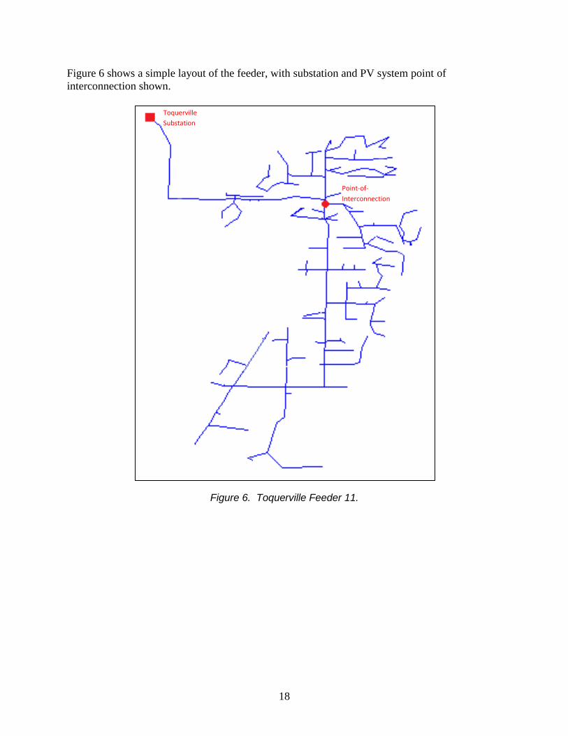
Figure 6 shows a simple layout of the feeder, with substation and PV system point of
interconnection shown.
Figure 6. Toquerville Feeder 11.
Toquerville
Substation
Point-of-
Interconnection
19
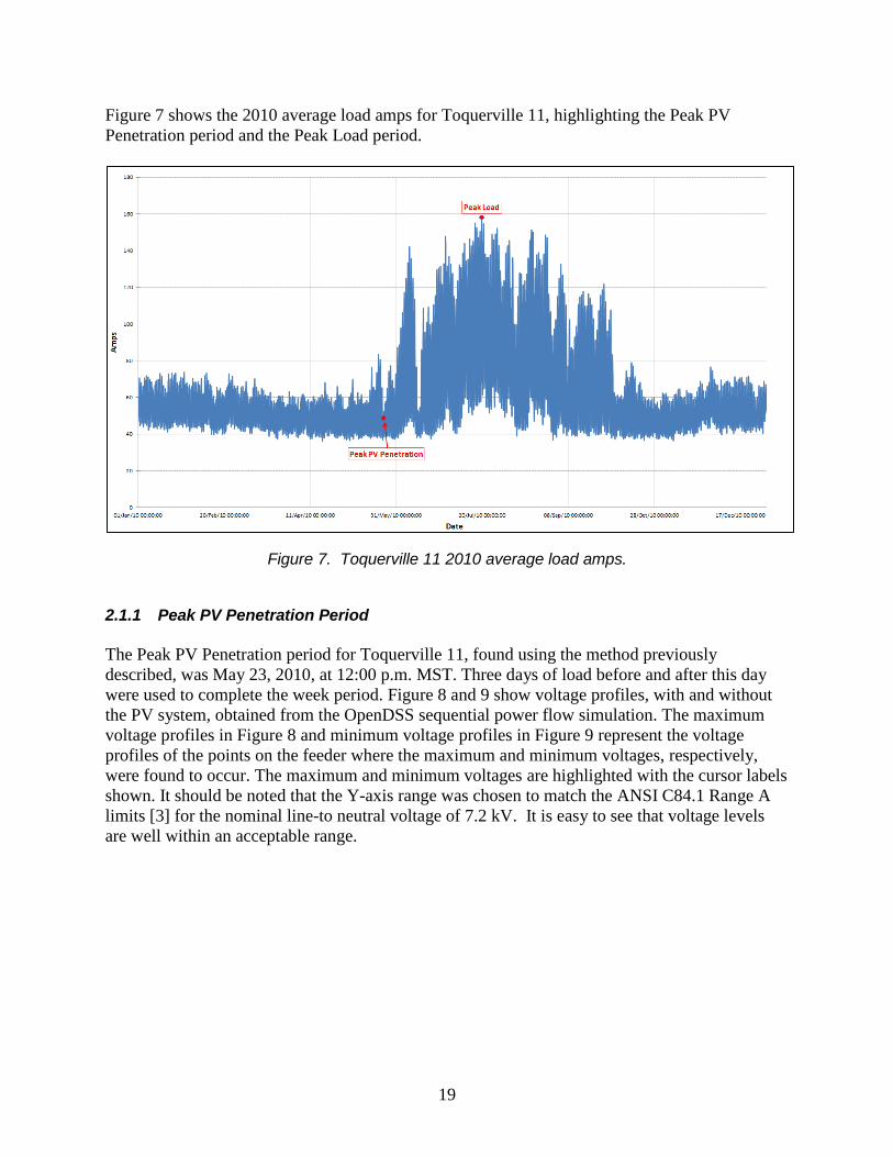
Figure 7 shows the 2010 average load amps for Toquerville 11, highlighting the Peak PV
Penetration period and the Peak Load period.
Figure 7. Toquerville 11 2010 average load amps.
2.1.1 Peak PV Penetration Period
The Peak PV Penetration period for Toquerville 11, found using the method previously
described, was May 23, 2010, at 12:00 p.m. MST. Three days of load before and after this day
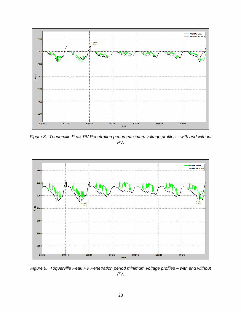
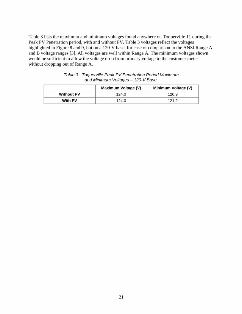
were used to complete the week period. Figure 8 and 9 show voltage profiles, with and without
the PV system, obtained from the OpenDSS sequential power flow simulation. The maximum
voltage profiles in Figure 8 and minimum voltage profiles in Figure 9 represent the voltage
profiles of the points on the feeder where the maximum and minimum voltages, respectively,
were found to occur. The maximum and minimum voltages are highlighted with the cursor labels
shown. It should be noted that the Y-axis range was chosen to match the ANSI C84.1 Range A
limits [3] for the nominal line-to neutral voltage of 7.2 kV. It is easy to see that voltage levels
are well within an acceptable range.
20
Figure 8. Toquerville Peak PV Penetration period maximum voltage profiles – with and without
PV.
Figure 9. Toquerville Peak PV Penetration period minimum voltage profiles – with and without
PV.
21
Table 3 lists the maximum and minimum voltages found anywhere on Toquerville 11 during the
Peak PV Penetration period, with and without PV. Table 3 voltages reflect the voltages
highlighted in Figure 8 and 9, but on a 120-V base, for ease of comparison to the ANSI Range A
and B voltage ranges [3]. All voltages are well within Range A. The minimum voltages shown
would be sufficient to allow the voltage drop from primary voltage to the customer meter
without dropping out of Range A.
Table 3. Toquerville Peak PV Penetration Period Maximum
and Minimum Voltages – 120-V Base.
Maximum Voltage (V) Minimum Voltage (V)
Without PV 124.0 120.9
With PV 124.0 121.2
22
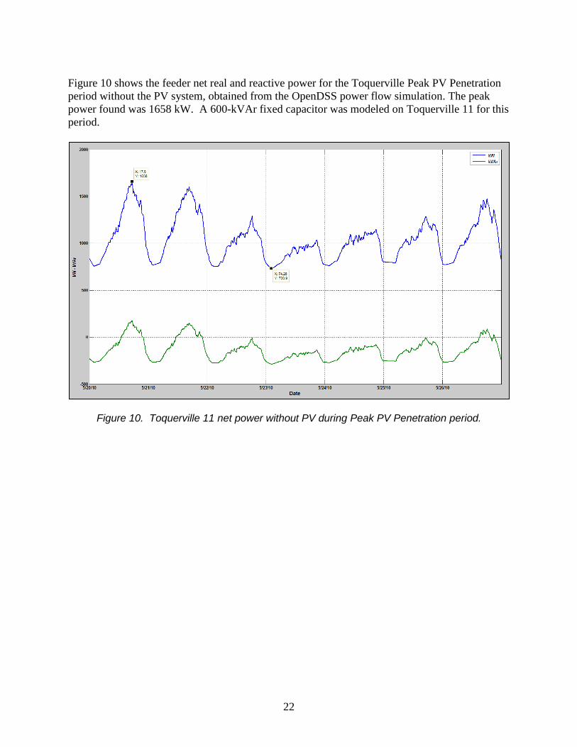
Figure 10 shows the feeder net real and reactive power for the Toquerville Peak PV Penetration
period without the PV system, obtained from the OpenDSS power flow simulation. The peak
power found was 1658 kW. A 600-kVAr fixed capacitor was modeled on Toquerville 11 for this
period.
Figure 10. Toquerville 11 net power without PV during Peak PV Penetration period.
23
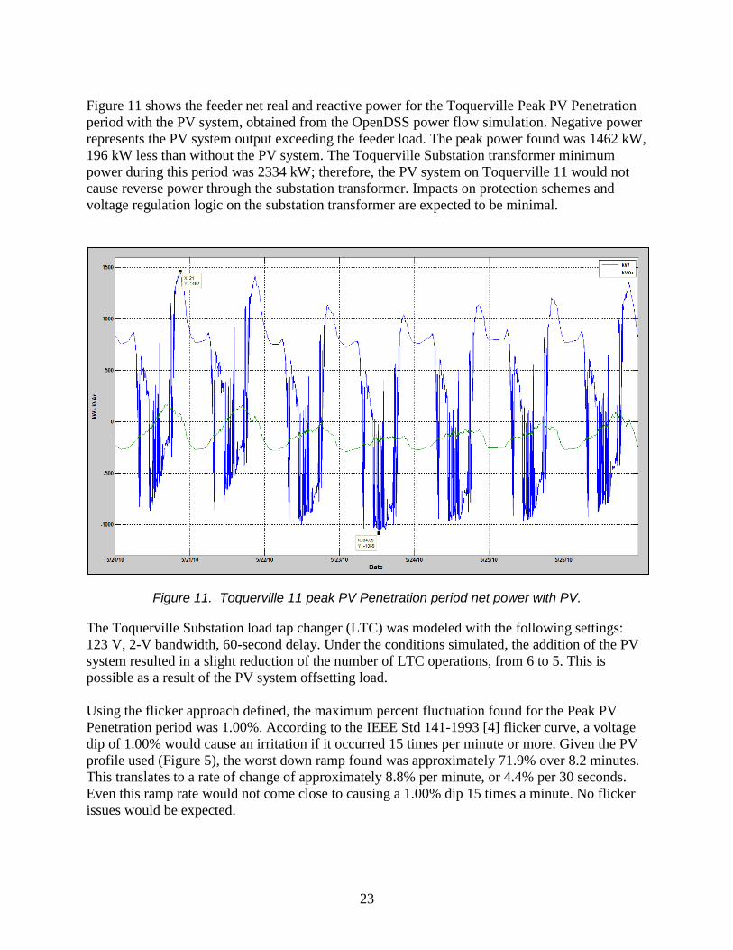
Figure 11 shows the feeder net real and reactive power for the Toquerville Peak PV Penetration
period with the PV system, obtained from the OpenDSS power flow simulation. Negative power
represents the PV system output exceeding the feeder load. The peak power found was 1462 kW,
196 kW less than without the PV system. The Toquerville Substation transformer minimum
power during this period was 2334 kW; therefore, the PV system on Toquerville 11 would not
cause reverse power through the substation transformer. Impacts on protection schemes and
voltage regulation logic on the substation transformer are expected to be minimal.
Figure 11. Toquerville 11 peak PV Penetration period net power with PV.
The Toquerville Substation load tap changer (LTC) was modeled with the following settings:
123 V, 2-V bandwidth, 60-second delay. Under the conditions simulated, the addition of the PV
system resulted in a slight reduction of the number of LTC operations, from 6 to 5. This is
possible as a result of the PV system offsetting load.
Using the flicker approach defined, the maximum percent fluctuation found for the Peak PV
Penetration period was 1.00%. According to the IEEE Std 141-1993 [4] flicker curve, a voltage
dip of 1.00% would cause an irritation if it occurred 15 times per minute or more. Given the PV
profile used (Figure 5), the worst down ramp found was approximately 71.9% over 8.2 minutes.
This translates to a rate of change of approximately 8.8% per minute, or 4.4% per 30 seconds.
Even this ramp rate would not come close to causing a 1.00% dip 15 times a minute. No flicker
issues would be expected.
24
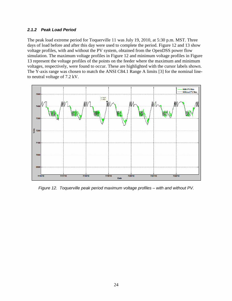
2.1.2 Peak Load Period
The peak load extreme period for Toquerville 11 was July 19, 2010, at 5:30 p.m. MST. Three
days of load before and after this day were used to complete the period. Figure 12 and 13 show
voltage profiles, with and without the PV system, obtained from the OpenDSS power flow
simulation. The maximum voltage profiles in Figure 12 and minimum voltage profiles in Figure
13 represent the voltage profiles of the points on the feeder where the maximum and minimum
voltages, respectively, were found to occur. These are highlighted with the cursor labels shown.
The Y-axis range was chosen to match the ANSI C84.1 Range A limits [3] for the nominal line-
to neutral voltage of 7.2 kV.
Figure 12. Toquerville peak period maximum voltage profiles – with and without PV.
25
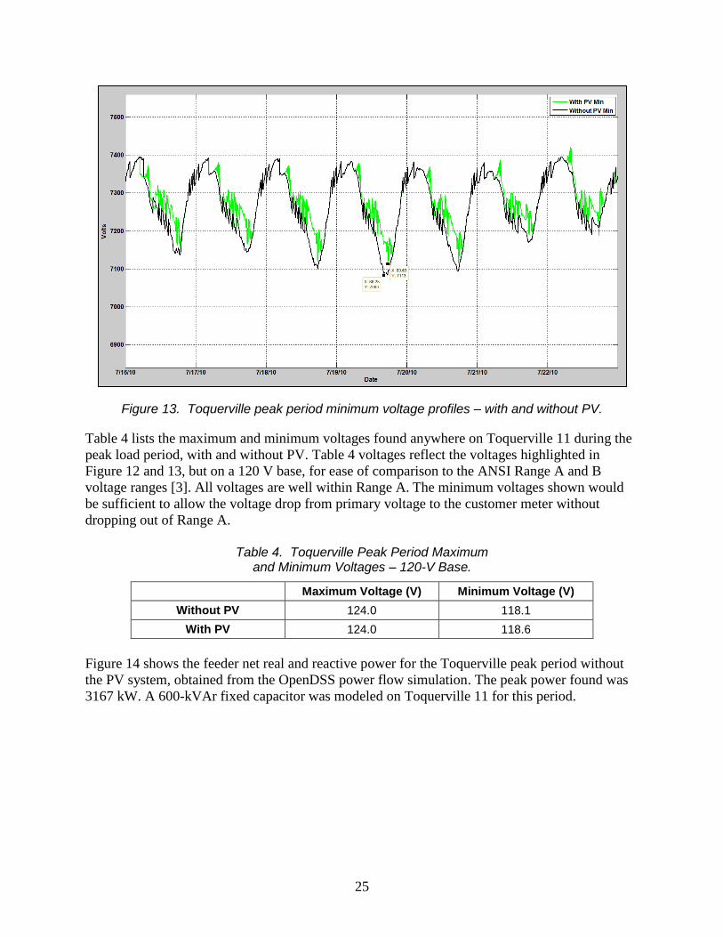
Figure 13. Toquerville peak period minimum voltage profiles – with and without PV.
Table 4 lists the maximum and minimum voltages found anywhere on Toquerville 11 during the
peak load period, with and without PV. Table 4 voltages reflect the voltages highlighted in
Figure 12 and 13, but on a 120 V base, for ease of comparison to the ANSI Range A and B
voltage ranges [3]. All voltages are well within Range A. The minimum voltages shown would
be sufficient to allow the voltage drop from primary voltage to the customer meter without
dropping out of Range A.
Table 4. Toquerville Peak Period Maximum
and Minimum Voltages – 120-V Base.
Maximum Voltage (V) Minimum Voltage (V)
Without PV 124.0 118.1
With PV 124.0 118.6
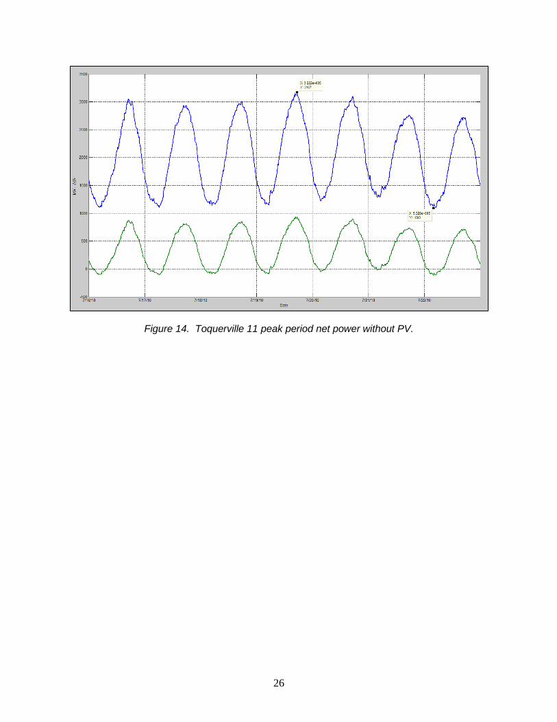
Figure 14 shows the feeder net real and reactive power for the Toquerville peak period without
the PV system, obtained from the OpenDSS power flow simulation. The peak power found was
3167 kW. A 600-kVAr fixed capacitor was modeled on Toquerville 11 for this period.
26
Figure 14. Toquerville 11 peak period net power without PV.
27
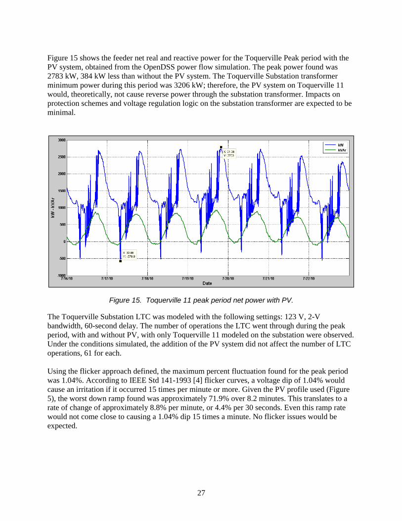
Figure 15 shows the feeder net real and reactive power for the Toquerville Peak period with the
PV system, obtained from the OpenDSS power flow simulation. The peak power found was
2783 kW, 384 kW less than without the PV system. The Toquerville Substation transformer
minimum power during this period was 3206 kW; therefore, the PV system on Toquerville 11
would, theoretically, not cause reverse power through the substation transformer. Impacts on
protection schemes and voltage regulation logic on the substation transformer are expected to be
minimal.
Figure 15. Toquerville 11 peak period net power with PV.
The Toquerville Substation LTC was modeled with the following settings: 123 V, 2-V
bandwidth, 60-second delay. The number of operations the LTC went through during the peak
period, with and without PV, with only Toquerville 11 modeled on the substation were observed.
Under the conditions simulated, the addition of the PV system did not affect the number of LTC
operations, 61 for each.
Using the flicker approach defined, the maximum percent fluctuation found for the peak period
was 1.04%. According to IEEE Std 141-1993 [4] flicker curves, a voltage dip of 1.04% would
cause an irritation if it occurred 15 times per minute or more. Given the PV profile used (Figure
5), the worst down ramp found was approximately 71.9% over 8.2 minutes. This translates to a
rate of change of approximately 8.8% per minute, or 4.4% per 30 seconds. Even this ramp rate
would not come close to causing a 1.04% dip 15 times a minute. No flicker issues would be
expected.

28
2.1.3 Toquerville 11 Summary
The Toquerville 11 2-MW PV system, approximately 63% of feeder peak load in 2010, did not
reveal any disputable impacts based on the study conducted. Table 5 is a consolidation of the
results found.
Table 5. Toquerville 11 Results Summary.
Peak PV Penetration Period Peak Period
Without PV With PV Without PV With PV
Maximum Voltage 124.0 124.0 124.0 124.0
Minimum Voltage 120.9 121.2 118.1 118.6
Peak Power (kW) 1658 1462 3167 2783
LTC Operations 6 5 61 61
Flicker Test Peak 1.00% 1.04%
2.2 Delta 11
Delta Substation is located in Delta, a small rural city in central Utah. The chosen PV site is
approximately 0.6 mile east of Delta Substation, as shown in Figure 16. A nominal 2-MW PV
system represents approximately 116% of peak load for Delta 11 in 2010.
Figure 16. Delta Feeder 11 PV plant location.
Delta Sub
2 MW PV Plant
29
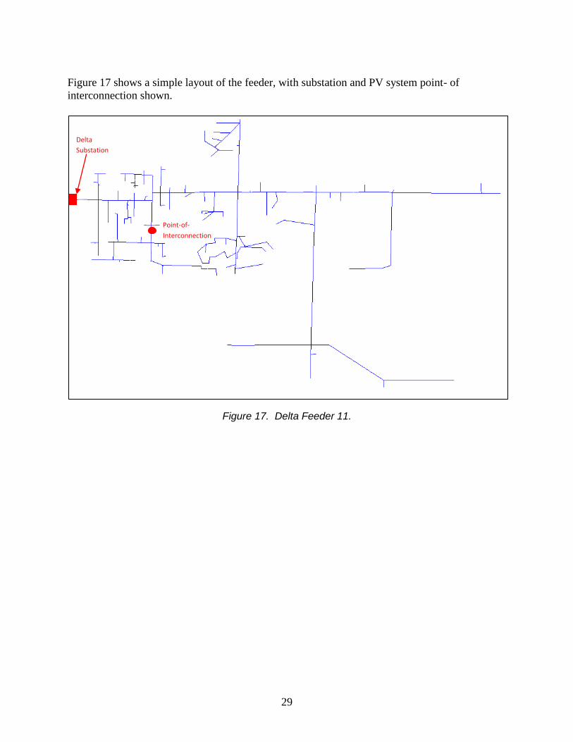
Figure 17 shows a simple layout of the feeder, with substation and PV system point- of
interconnection shown.
Figure 17. Delta Feeder 11.
Delta
Substation
Point-of-
Interconnection
30
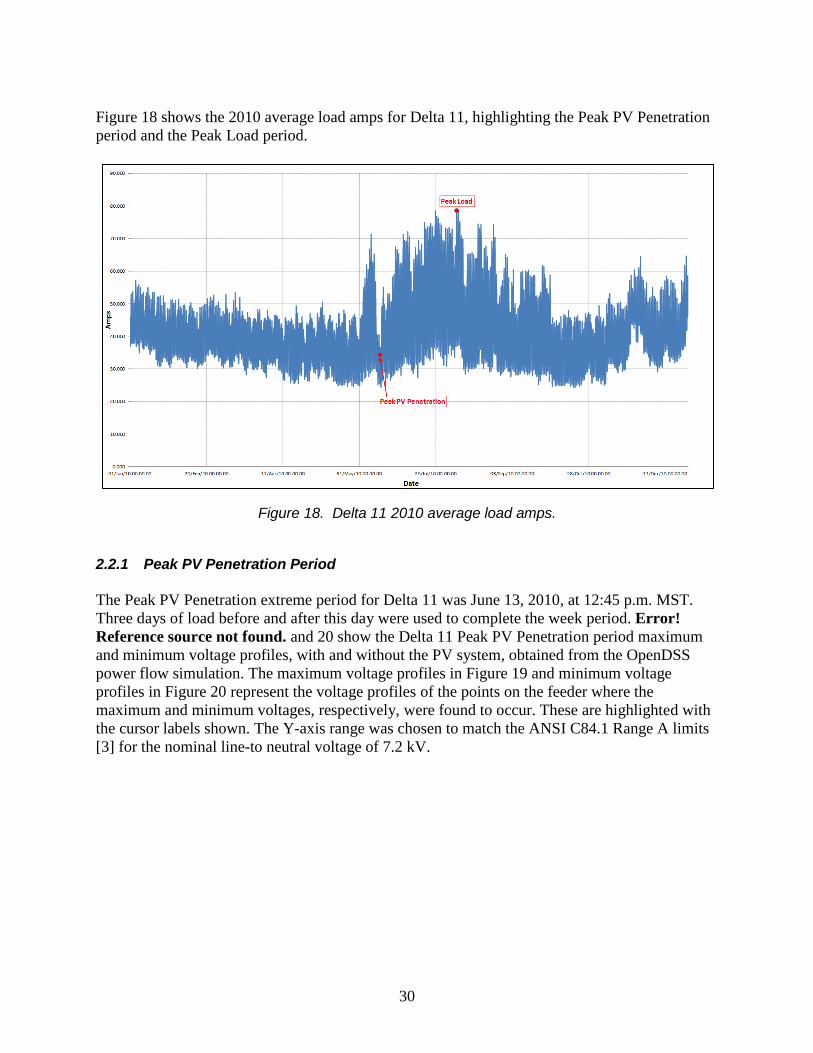
Figure 18 shows the 2010 average load amps for Delta 11, highlighting the Peak PV Penetration
period and the Peak Load period.
Figure 18. Delta 11 2010 average load amps.
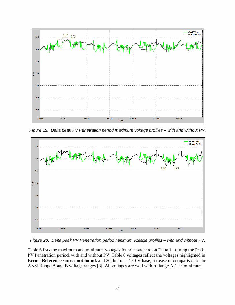
2.2.1 Peak PV Penetration Period
The Peak PV Penetration extreme period for Delta 11 was June 13, 2010, at 12:45 p.m. MST.
Three days of load before and after this day were used to complete the week period. Error!
Reference source not found. and 20 show the Delta 11 Peak PV Penetration period maximum
and minimum voltage profiles, with and without the PV system, obtained from the OpenDSS
power flow simulation. The maximum voltage profiles in Figure 19 and minimum voltage
profiles in Figure 20 represent the voltage profiles of the points on the feeder where the
maximum and minimum voltages, respectively, were found to occur. These are highlighted with
the cursor labels shown. The Y-axis range was chosen to match the ANSI C84.1 Range A limits
[3] for the nominal line-to neutral voltage of 7.2 kV.
31
Figure 19. Delta peak PV Penetration period maximum voltage profiles – with and without PV.
Figure 20. Delta peak PV Penetration period minimum voltage profiles – with and without PV.
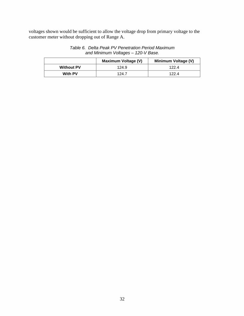
Table 6 lists the maximum and minimum voltages found anywhere on Delta 11 during the Peak
PV Penetration period, with and without PV. Table 6 voltages reflect the voltages highlighted in
Error! Reference source not found. and 20, but on a 120-V base, for ease of comparison to the
ANSI Range A and B voltage ranges [3]. All voltages are well within Range A. The minimum
32
voltages shown would be sufficient to allow the voltage drop from primary voltage to the
customer meter without dropping out of Range A.
Table 6. Delta Peak PV Penetration Period Maximum
and Minimum Voltages – 120-V Base.
Maximum Voltage (V) Minimum Voltage (V)
Without PV 124.9 122.4
With PV 124.7 122.4

33
Figure 21 shows the feeder net real and reactive power for the Delta Peak PV Penetration period
without the PV system, obtained from the OpenDSS power flow simulation. The peak power
found was 1246 kW. Two 300-kVAr fixed capacitors were modeled on Delta 11 for this period.
Figure 21. Delta 11 Peak PV Penetration period net power without PV.
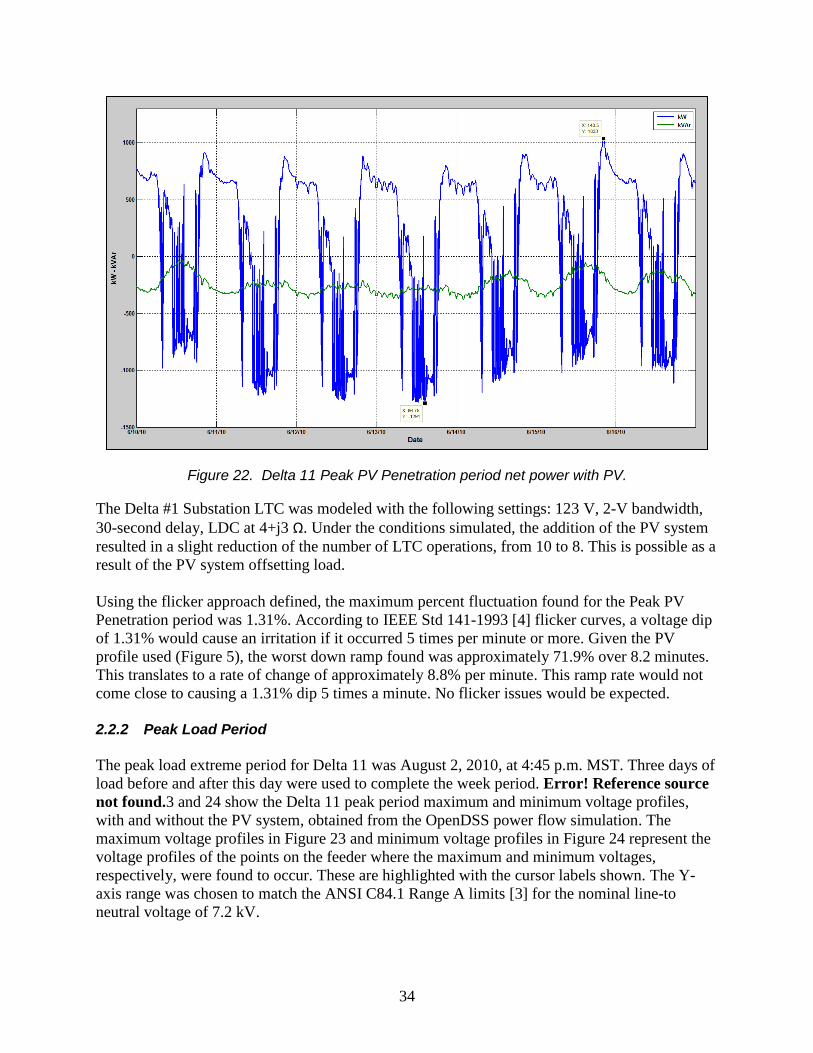
Figure 22 shows the feeder net real and reactive power for the Delta Peak PV Penetration
period with the PV system, obtained from the OpenDSS power flow simulation. Negative
power represents the PV system output exceeding the feeder load. The peak power found was
-1291 kW, 45 kW greater than without the PV system. Note the higher peak was due to the PV
system output exceeding the load on June 13, 2010, at an amount greater than the load peak for
the period on June 10, 2010 (Figure 21). The Delta Substation transformer minimum power
during this period was 3626 kW; therefore, the PV system on Delta 11 would, theoretically, not
cause reverse power through the substation transformer. Impacts on protection schemes and
voltage regulation logic on the substation transformer are expected to be minimal.
34
Figure 22. Delta 11 Peak PV Penetration period net power with PV.
The Delta #1 Substation LTC was modeled with the following settings: 123 V, 2-V bandwidth,
30-second delay, LDC at 4+j3 Ω. Under the conditions simulated, the addition of the PV system
resulted in a slight reduction of the number of LTC operations, from 10 to 8. This is possible as a
result of the PV system offsetting load.
Using the flicker approach defined, the maximum percent fluctuation found for the Peak PV
Penetration period was 1.31%. According to IEEE Std 141-1993 [4] flicker curves, a voltage dip
of 1.31% would cause an irritation if it occurred 5 times per minute or more. Given the PV
profile used (Figure 5), the worst down ramp found was approximately 71.9% over 8.2 minutes.
This translates to a rate of change of approximately 8.8% per minute. This ramp rate would not
come close to causing a 1.31% dip 5 times a minute. No flicker issues would be expected.
2.2.2 Peak Load Period
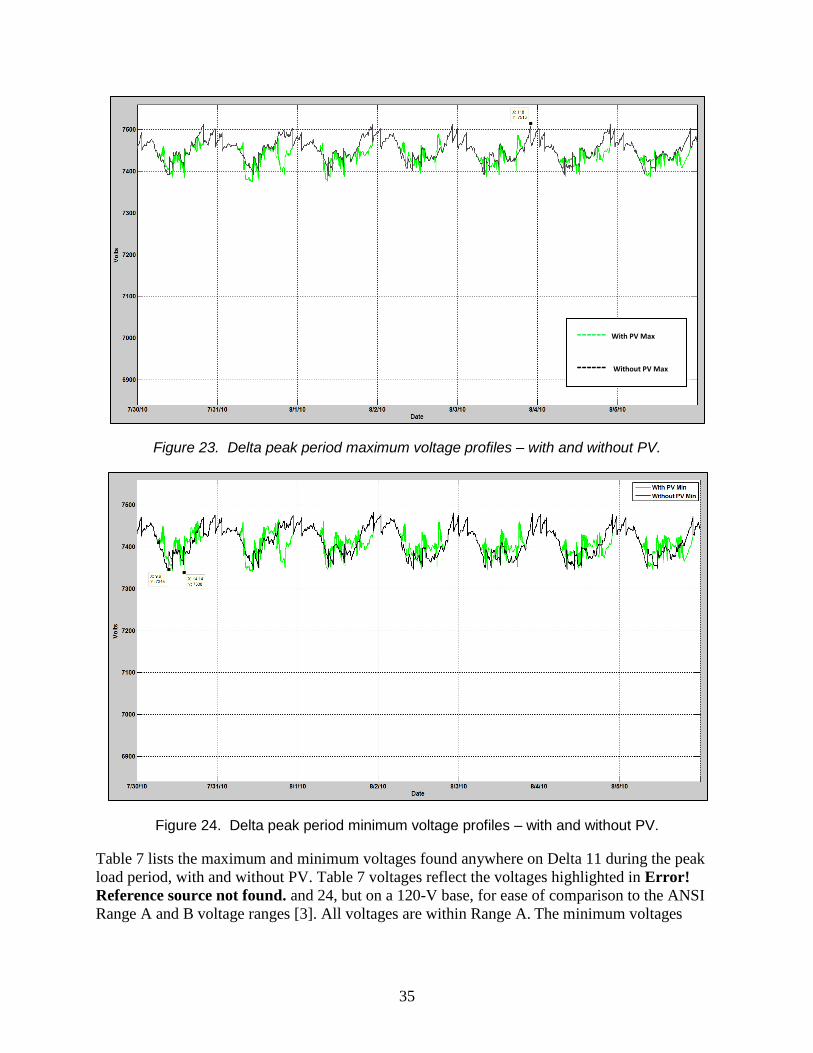
The peak load extreme period for Delta 11 was August 2, 2010, at 4:45 p.m. MST. Three days of
load before and after this day were used to complete the week period. Error! Reference source
not found.3 and 24 show the Delta 11 peak period maximum and minimum voltage profiles,
with and without the PV system, obtained from the OpenDSS power flow simulation. The
maximum voltage profiles in Figure 23 and minimum voltage profiles in Figure 24 represent the
voltage profiles of the points on the feeder where the maximum and minimum voltages,
respectively, were found to occur. These are highlighted with the cursor labels shown. The Y-
axis range was chosen to match the ANSI C84.1 Range A limits [3] for the nominal line-to
neutral voltage of 7.2 kV.
35
Figure 23. Delta peak period maximum voltage profiles – with and without PV.
Figure 24. Delta peak period minimum voltage profiles – with and without PV.
Table 7 lists the maximum and minimum voltages found anywhere on Delta 11 during the peak
load period, with and without PV. Table 7 voltages reflect the voltages highlighted in Error!
Reference source not found. and 24, but on a 120-V base, for ease of comparison to the ANSI
Range A and B voltage ranges [3]. All voltages are within Range A. The minimum voltages
------ With PV Max
------ Without PV Max

36
shown would be sufficient to allow the voltage drop from primary voltage to the customer meter
without dropping out of Range A.
Table 7. Delta Peak Period Maximum and Minimum Voltages – 120-V Base.
Maximum Voltage (V) Minimum Voltage (V)
Without PV 125.2 122.4
With PV 125.2 122.3
37
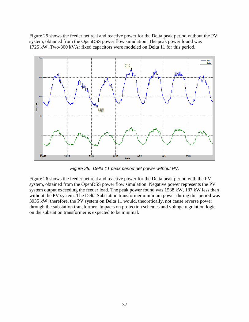
Figure 25 shows the feeder net real and reactive power for the Delta peak period without the PV
system, obtained from the OpenDSS power flow simulation. The peak power found was
1725 kW. Two-300 kVAr fixed capacitors were modeled on Delta 11 for this period.
Figure 25. Delta 11 peak period net power without PV.
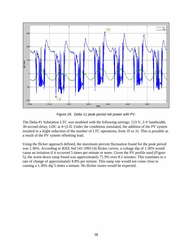
Figure 26 shows the feeder net real and reactive power for the Delta peak period with the PV
system, obtained from the OpenDSS power flow simulation. Negative power represents the PV
system output exceeding the feeder load. The peak power found was 1538 kW, 187 kW less than
without the PV system. The Delta Substation transformer minimum power during this period was
3935 kW; therefore, the PV system on Delta 11 would, theoretically, not cause reverse power
through the substation transformer. Impacts on protection schemes and voltage regulation logic
on the substation transformer is expected to be minimal.
38
Figure 26. Delta 11 peak period net power with PV.
The Delta #1 Substation LTC was modeled with the following settings: 123 V, 2-V bandwidth,
30-second delay, LDC at 4+j3 Ω. Under the conditions simulated, the addition of the PV system
resulted in a slight reduction of the number of LTC operations, from 35 to 31. This is possible as
a result of the PV system offsetting load.
Using the flicker approach defined, the maximum percent fluctuation found for the peak period
was 1.36%. According to IEEE Std 141-1993 [4] flicker curves, a voltage dip of 1.36% would
cause an irritation if it occurred 5 times per minute or more. Given the PV profile used (Figure
5), the worst down ramp found was approximately 71.9% over 8.2 minutes. This translates to a
rate of change of approximately 8.8% per minute. This ramp rate would not come close to
causing a 1.36% dip 5 times a minute. No flicker issues would be expected.
39
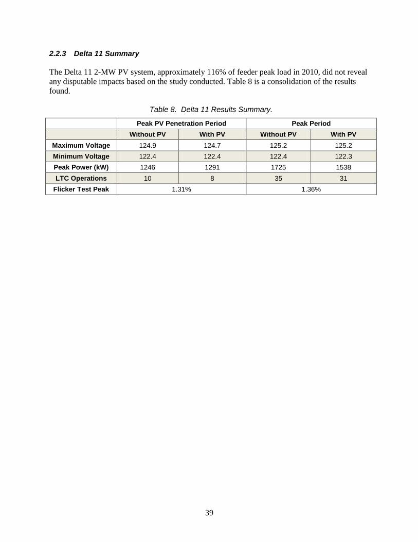
2.2.3 Delta 11 Summary
The Delta 11 2-MW PV system, approximately 116% of feeder peak load in 2010, did not reveal
any disputable impacts based on the study conducted. Table 8 is a consolidation of the results
found.
Table 8. Delta 11 Results Summary.
Peak PV Penetration Period Peak Period
Without PV With PV Without PV With PV
Maximum Voltage 124.9 124.7 125.2 125.2
Minimum Voltage 122.4 122.4 122.4 122.3
Peak Power (kW) 1246 1291 1725 1538
LTC Operations 10 8 35 31
Flicker Test Peak 1.31% 1.36%
40
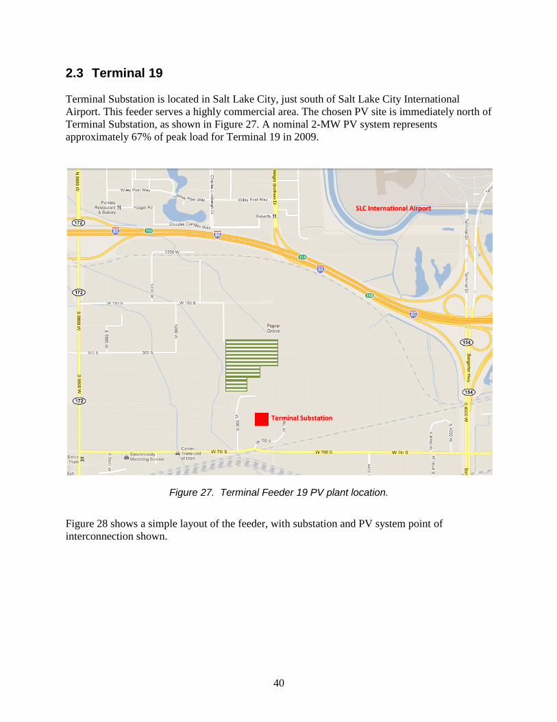
2.3 Terminal 19
Terminal Substation is located in Salt Lake City, just south of Salt Lake City International
Airport. This feeder serves a highly commercial area. The chosen PV site is immediately north of
Terminal Substation, as shown in Figure 27. A nominal 2-MW PV system represents
approximately 67% of peak load for Terminal 19 in 2009.
Figure 27. Terminal Feeder 19 PV plant location.
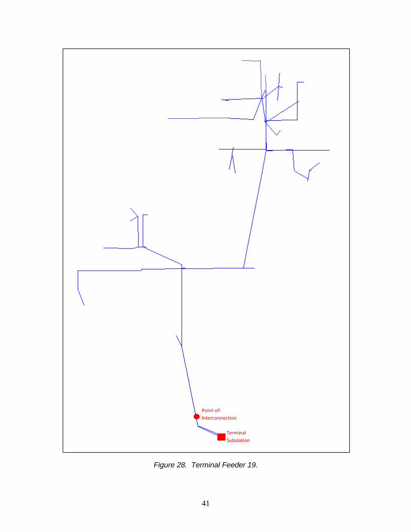
Figure 28 shows a simple layout of the feeder, with substation and PV system point of
interconnection shown.
Terminal Substation
SLC International Airport
41
Figure 28. Terminal Feeder 19.
Terminal
Substation
Point-of-
Interconnection
42
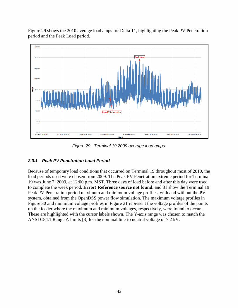
Figure 29 shows the 2010 average load amps for Delta 11, highlighting the Peak PV Penetration
period and the Peak Load period.
Figure 29. Terminal 19 2009 average load amps.
2.3.1 Peak PV Penetration Load Period
Because of temporary load conditions that occurred on Terminal 19 throughout most of 2010, the
load periods used were chosen from 2009. The Peak PV Penetration extreme period for Terminal
19 was June 7, 2009, at 12:00 p.m. MST. Three days of load before and after this day were used
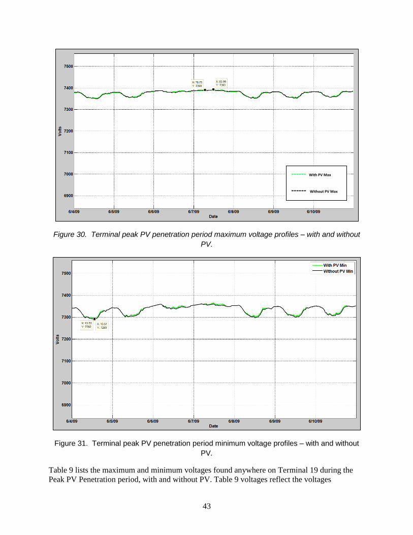
to complete the week period. Error! Reference source not found. and 31 show the Terminal 19
Peak PV Penetration period maximum and minimum voltage profiles, with and without the PV
system, obtained from the OpenDSS power flow simulation. The maximum voltage profiles in
Figure 30 and minimum voltage profiles in Figure 31 represent the voltage profiles of the points
on the feeder where the maximum and minimum voltages, respectively, were found to occur.
These are highlighted with the cursor labels shown. The Y-axis range was chosen to match the
ANSI C84.1 Range A limits [3] for the nominal line-to neutral voltage of 7.2 kV.
43
Figure 30. Terminal peak PV penetration period maximum voltage profiles – with and without
PV.
Figure 31. Terminal peak PV penetration period minimum voltage profiles – with and without
PV.
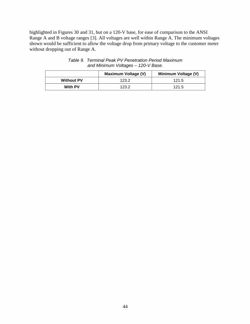
Table 9 lists the maximum and minimum voltages found anywhere on Terminal 19 during the
Peak PV Penetration period, with and without PV. Table 9 voltages reflect the voltages
------ With PV Max
------ Without PV Max
44
highlighted in Figures 30 and 31, but on a 120-V base, for ease of comparison to the ANSI
Range A and B voltage ranges [3]. All voltages are well within Range A. The minimum voltages
shown would be sufficient to allow the voltage drop from primary voltage to the customer meter
without dropping out of Range A.
Table 9. Terminal Peak PV Penetration Period Maximum
and Minimum Voltages – 120-V Base.
Maximum Voltage (V) Minimum Voltage (V)
Without PV 123.2 121.5
With PV 123.2 121.5
45
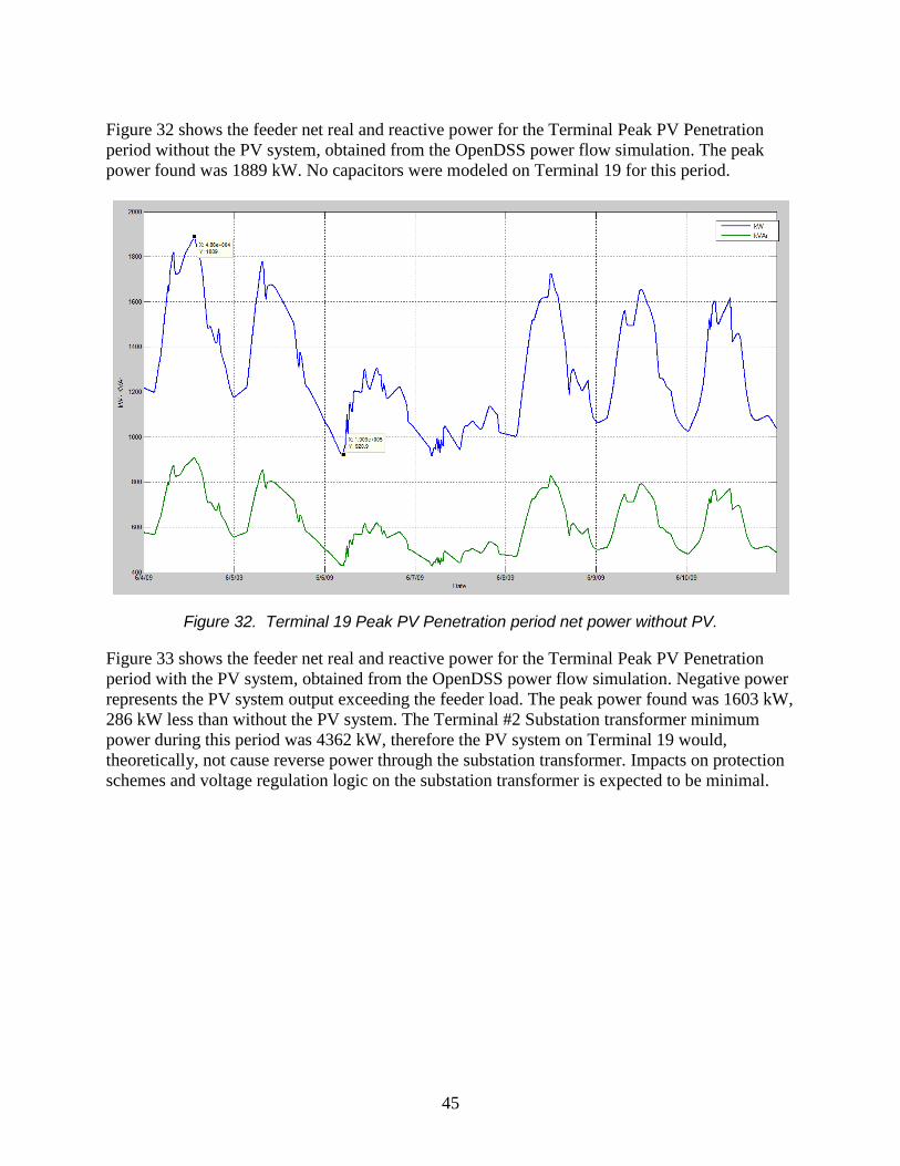
Figure 32 shows the feeder net real and reactive power for the Terminal Peak PV Penetration
period without the PV system, obtained from the OpenDSS power flow simulation. The peak
power found was 1889 kW. No capacitors were modeled on Terminal 19 for this period.
Figure 32. Terminal 19 Peak PV Penetration period net power without PV.
Figure 33 shows the feeder net real and reactive power for the Terminal Peak PV Penetration
period with the PV system, obtained from the OpenDSS power flow simulation. Negative power
represents the PV system output exceeding the feeder load. The peak power found was 1603 kW,
286 kW less than without the PV system. The Terminal #2 Substation transformer minimum
power during this period was 4362 kW, therefore the PV system on Terminal 19 would,
theoretically, not cause reverse power through the substation transformer. Impacts on protection
schemes and voltage regulation logic on the substation transformer is expected to be minimal.
46
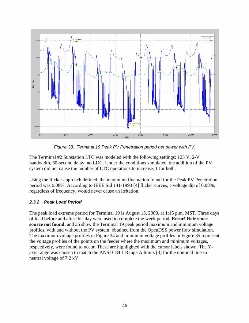
Figure 33. Terminal 19 Peak PV Penetration period net power with PV.
The Terminal #2 Substation LTC was modeled with the following settings: 123 V, 2-V
bandwidth, 60-second delay, no LDC. Under the conditions simulated, the addition of the PV
system did not cause the number of LTC operations to increase, 1 for both.
Using the flicker approach defined, the maximum fluctuation found for the Peak PV Penetration
period was 0.08%. According to IEEE Std 141-1993 [4] flicker curves, a voltage dip of 0.08%,
regardless of frequency, would never cause an irritation.
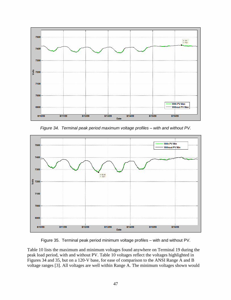
2.3.2 Peak Load Period
The peak load extreme period for Terminal 19 is August 13, 2009, at 1:15 p.m. MST. Three days
of load before and after this day were used to complete the week period. Error! Reference
source not found. and 35 show the Terminal 19 peak period maximum and minimum voltage
profiles, with and without the PV system, obtained from the OpenDSS power flow simulation.
The maximum voltage profiles in Figure 34 and minimum voltage profiles in Figure 35 represent
the voltage profiles of the points on the feeder where the maximum and minimum voltages,
respectively, were found to occur. These are highlighted with the cursor labels shown. The Y-
axis range was chosen to match the ANSI C84.1 Range A limits [3] for the nominal line-to
neutral voltage of 7.2 kV.
47
Figure 34. Terminal peak period maximum voltage profiles – with and without PV.
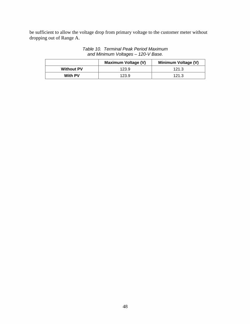
Figure 35. Terminal peak period minimum voltage profiles – with and without PV.
Table 10 lists the maximum and minimum voltages found anywhere on Terminal 19 during the
peak load period, with and without PV. Table 10 voltages reflect the voltages highlighted in
Figures 34 and 35, but on a 120-V base, for ease of comparison to the ANSI Range A and B
voltage ranges [3]. All voltages are well within Range A. The minimum voltages shown would
48
be sufficient to allow the voltage drop from primary voltage to the customer meter without
dropping out of Range A.
Table 10. Terminal Peak Period Maximum
and Minimum Voltages – 120-V Base.
Maximum Voltage (V) Minimum Voltage (V)
Without PV 123.9 121.3
With PV 123.9 121.3
49
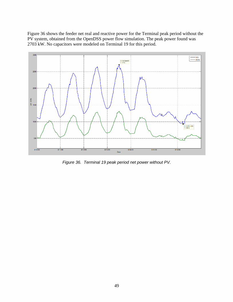
Figure 36 shows the feeder net real and reactive power for the Terminal peak period without the
PV system, obtained from the OpenDSS power flow simulation. The peak power found was
2703 kW. No capacitors were modeled on Terminal 19 for this period.
Figure 36. Terminal 19 peak period net power without PV.

50
Figure 37 shows the feeder net real and reactive power for the Terminal peak period with the PV
system, obtained from the OpenDSS power flow simulation. Negative power represents the PV
system output exceeding the feeder load. The peak power found was 2087 kW, 616 kW less than
without the PV system. The Terminal #2 Substation transformer minimum power during this
period was 4311 kW; therefore, the PV system on Terminal 19 would, theoretically, not cause
reverse power through the substation transformer. Impacts on protection schemes and voltage
regulation logic on the substation transformer is expected to be minimal.
Figure 37. Terminal 19 peak period net power with PV.
The Terminal #2 Substation LTC was modeled with the following settings: 123 V, 2-V
bandwidth, 60-second delay, no LDC. Under the conditions simulated, the addition of the PV
system did not cause the number of LTC operations to increase, 2 for both.
Using the flicker approach defined, the maximum fluctuation found for the peak period was
0.09%. According to IEEE Std 141-1993 [4] flicker curves, a voltage dip of 0.09%, regardless of
frequency, would never cause an irritation.

51
2.3.3 Terminal 19 Summary
The Terminal 19 2-MW PV system, approximately 67% of feeder peak load in 2009, did not
reveal any disputable impacts based on the study conducted. Table 11 is a consolidation of the
results found.
Table 11. Terminal 19 Results Summary.
Peak PV Penetration Period Peak Period
Without PV With PV Without PV With PV
Maximum Voltage 123.2 123.2 123.8 123.8
Minimum Voltage 121.5 121.5 121.3 121.3
Peak Power (kW) 1889 1603 2703 2087
LTC Operations 11 1 2 2
Flicker Test Peak 0.08% 0.09%

52
3 PERFORMANCE MODELING
3.1 Solar System Designs
Three system designs were established for the project: a fixed-tilt multicrystalline silicon system,
a fixed-tilt thin-film system, and a one-axis tracking (east to west) multicrystalline system. Each
system has a nominal size of 2 MWac.
The fixed-tilt multicrystalline system is the baseline system and contains the most commonly
used technology. The other two systems are variations of that design. The fixed-tilt thin-film
system uses thin-film CdTe modules, which are lower efficiency. The third system uses the same
modules as the baseline system, but the modules are mounted on one-axis trackers to enhance
energy production.
The system designs were prepared by an Albuquerque-based systems integrator with experience
building projects in the MW size range. These designs were evolutions of their standard designs.
The components used in the systems and the system designs are summarized in Table 12. Color
coding is used to show where two or more of the designs share the same features.
53
Table 12. System Designs.
Technology CdTe Thin-Film Multicrystalline Silicon
Structure Fixed Tilt Fixed Tilt 1-axis E-W tracking
Rating STC/PTC 75 W ±5% / 72.2 W 230 W ±3% / 206.6 W 230 W ±3% / 206.6 W
Size (m) 1.2 x 0.6 1.65 x 0.99 1.65 x 0.99
Efficiency STC/PTC 10.42% / 10.03% 14.08% / 12.65% 14.08% / 12.65%
Pmp Temp. Coefficient -0.25%/°C -0.45%/°C -0.45%/°C
Open-Circuit Voltage 89.6 V 37.0 V 37.0 V
Total modules #/Wp 28,800 / 2,160,000 9,408 / 2,163,840 9,408 / 2,163,840
Total module area 20,736 m2 15,368 m
2 15,368 m
2
Modules per string 5 14 14
Strings per rack 12 2 2
Strings per system 5,760 672 672
Module Orientation Landscape Landscape Portrait
Configuration 10 Rows x 6 Columns 7 Rows x 4 Columns 1 Row x 28 Columns
Orientation South facing South facing N-S axis, E to W tracking
Tilt Fixed 30° Tilt Fixed 30° Tilt ±45° with back-tracking
Total Racks 480 336 336
Subarrays 8 with One Inverter
each 8 with One Inverter
each 8 with One Inverter
each
Rating 250 kWp 250 kWp 250 kWp
CEC Weighted Efficiency
97% 97% 97%
Fence
Perimeter ft/m 3,332 / 1,016 2,818 / 859 3,247 / 890
Area ft2/m
2 692,779 / 64,361 488,737 / 45,405 648,401 / 60,238
STC = Standard Test Conditions; PTC = PVUSA Test Conditions; CEC = California Energy Commission; Pmp = Maximum Power Point
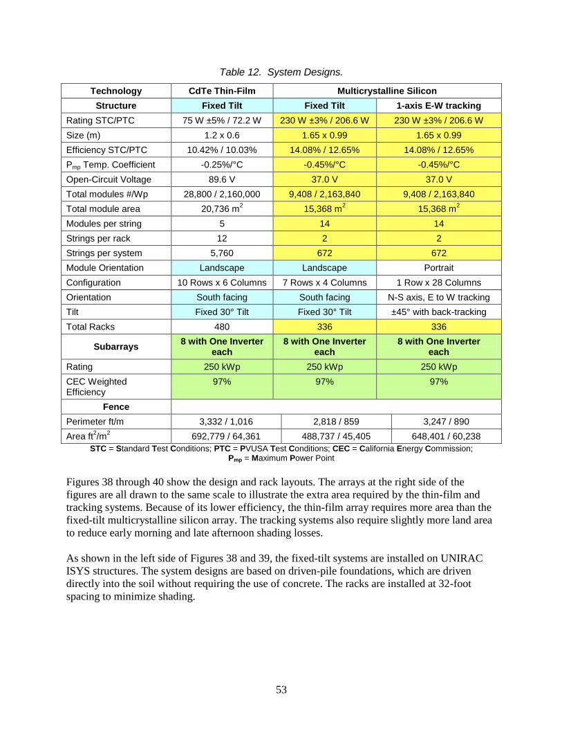
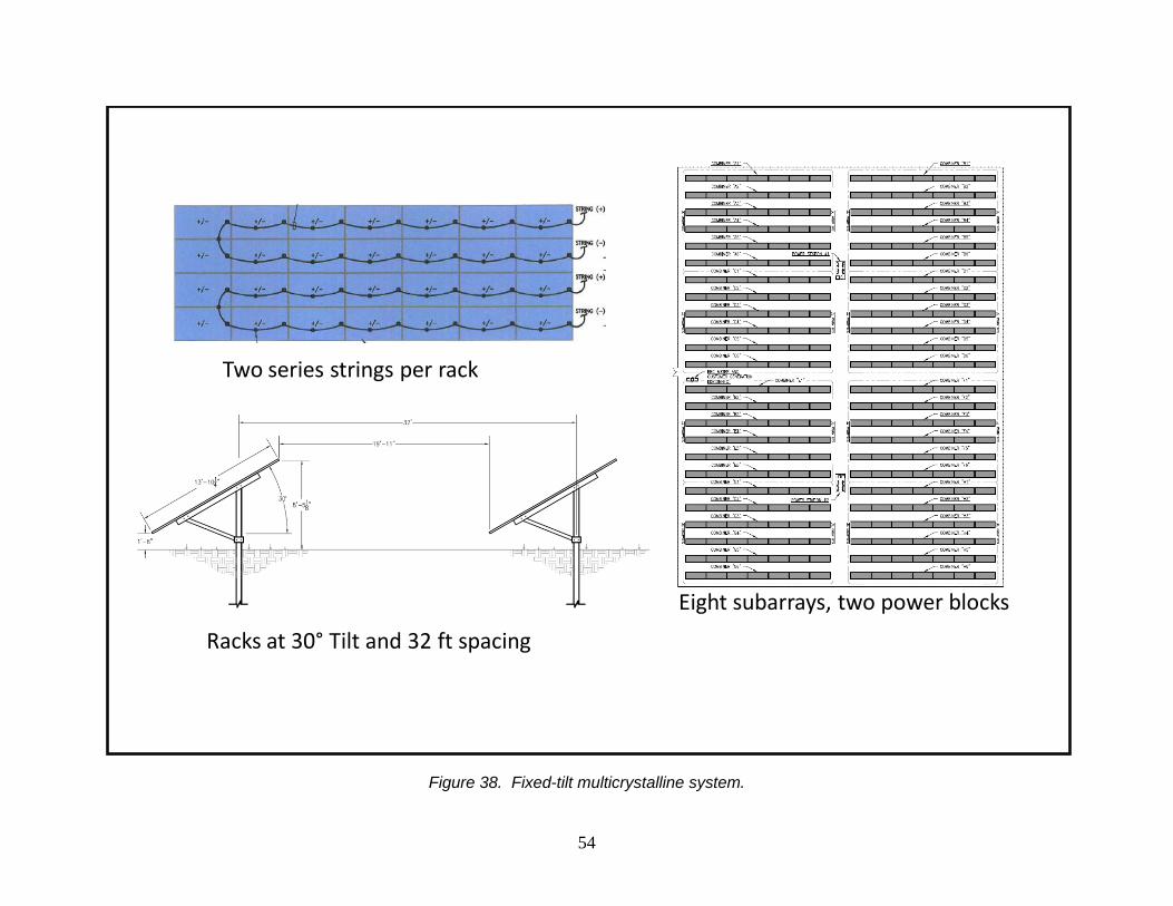
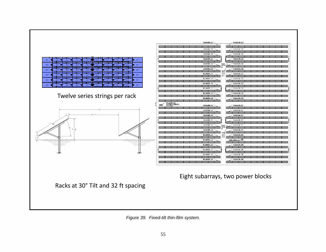
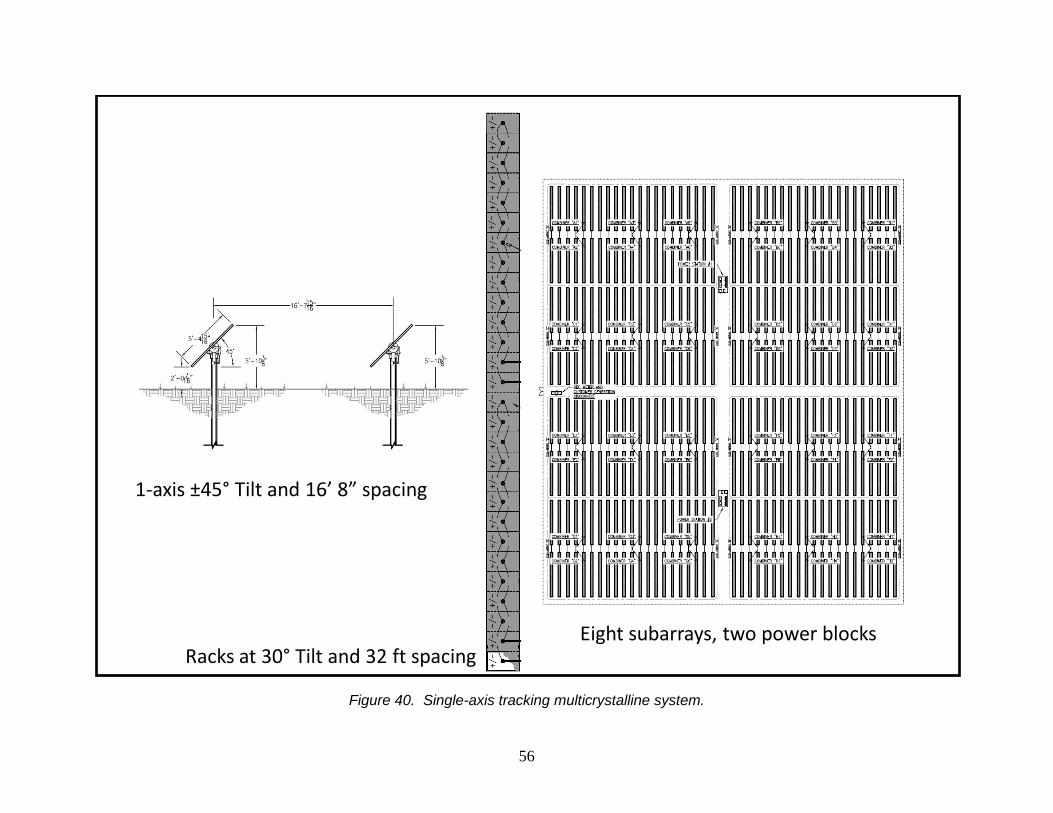
Figures 38 through 40 show the design and rack layouts. The arrays at the right side of the
figures are all drawn to the same scale to illustrate the extra area required by the thin-film and
tracking systems. Because of its lower efficiency, the thin-film array requires more area than the
fixed-tilt multicrystalline silicon array. The tracking systems also require slightly more land area
to reduce early morning and late afternoon shading losses.
As shown in the left side of Figures 38 and 39, the fixed-tilt systems are installed on UNIRAC
ISYS structures. The system designs are based on driven-pile foundations, which are driven
directly into the soil without requiring the use of concrete. The racks are installed at 32-foot
spacing to minimize shading.
54
Figure 38. Fixed-tilt multicrystalline system.
Two series strings per rack
Racks at 30° Tilt and 32 ft spacing
Multicrystalline silicon , fixed tilt system
Eight subarrays, two power blocks
55
Figure 39. Fixed-tilt thin-film system.
Twelve series strings per rack
Racks at 30° Tilt and 32 ft spacing
Thin-film, fixed tilt system
Eight subarrays, two power blocks
56
Figure 40. Single-axis tracking multicrystalline system.
Eight subarrays, two power blocks
1-axis ±45° Tilt and 16’ 8” spacing
Racks at 30° Tilt and 32 ft spacing
Multicrystalline silicon , 1-axis tracking system
57
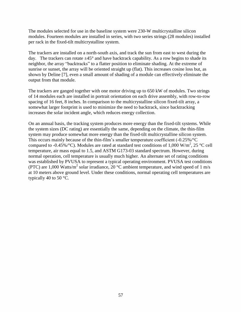
The modules selected for use in the baseline system were 230-W multicrystalline silicon
modules. Fourteen modules are installed in series, with two series strings (28 modules) installed
per rack in the fixed-tilt multicrystalline system.
The trackers are installed on a north-south axis, and track the sun from east to west during the
day. The trackers can rotate ±45° and have backtrack capability. As a row begins to shade its
neighbor, the array “backtracks” to a flatter position to eliminate shading. At the extreme of
sunrise or sunset, the array will be oriented straight up (flat). This increases cosine loss but, as
shown by Deline [7], even a small amount of shading of a module can effectively eliminate the
output from that module.
The trackers are ganged together with one motor driving up to 650 kW of modules. Two strings
of 14 modules each are installed in portrait orientation on each drive assembly, with row-to-row
spacing of 16 feet, 8 inches. In comparison to the multicrystalline silicon fixed-tilt array, a
somewhat larger footprint is used to minimize the need to backtrack, since backtracking
increases the solar incident angle, which reduces energy collection.
On an annual basis, the tracking system produces more energy than the fixed-tilt systems. While
the system sizes (DC rating) are essentially the same, depending on the climate, the thin-film
system may produce somewhat more energy than the fixed-tilt multicrystalline silicon system.
This occurs mainly because of the thin-film’s smaller temperature coefficient (-0.25%/°C
compared to -0.45%/°C). Modules are rated at standard test conditions of 1,000 W/m2, 25 °C cell
temperature, air mass equal to 1.5, and ASTM G173-03 standard spectrum. However, during
normal operation, cell temperature is usually much higher. An alternate set of rating conditions
was established by PVUSA to represent a typical operating environment. PVUSA test conditions
(PTC) are 1,000 Watts/m2 solar irradiance, 20 °C ambient temperature, and wind speed of 1 m/s
at 10 meters above ground level. Under these conditions, normal operating cell temperatures are
typically 40 to 50 °C.
58
3.2 Analytical Approach 3.2.1 Performance Analysis
Performance was simulated with the hourly simulation program, PVsyst [2]. PVsyst was selected
because of its ability to model shading and tracking in large systems. For the fixed-tilt arrays,
shading was analyzed using the unlimited shed option, which simplifies analysis by ignoring the
fact that the far east ends of the rows are not shaded in the morning and the far west ends are not
shaded in the afternoon. Tracking limits of ±45° with backtracking were used for the one-axis
tracking array.
The TMY-2 weather data were obtained from the Solar Prospector site
(http://maps.nrel.gov/prospector) for the following locations:
Toquerville, 37.25 N, -113.25 W
Terminal, 40.75 N, - 112.05 W
Delta, 39.35 N, -112.55 W
3.3 Results
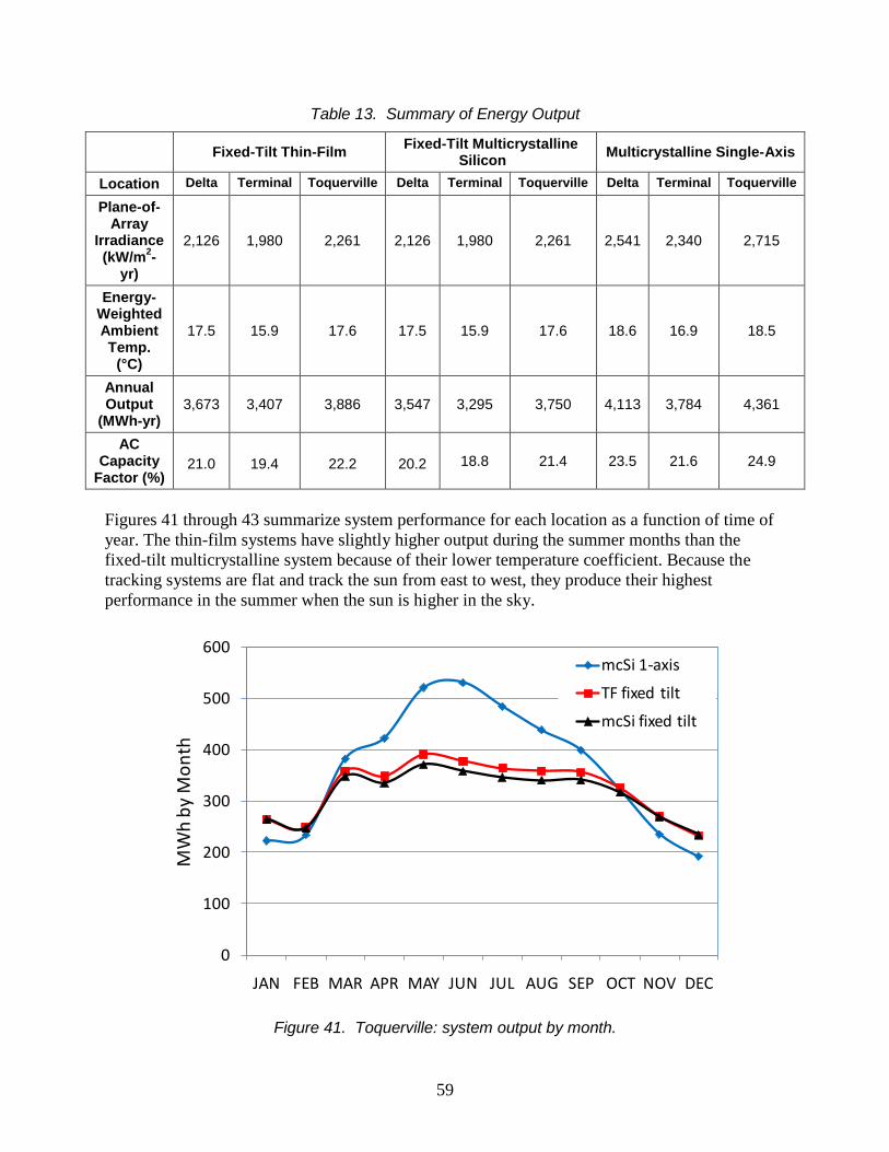
Table 13 provides a summary of system performance for fixed-tilt thin-film, fixed-tilt
multicrystalline silicon, and multicrystalline single-axis, respectively, for the three locations. The
capacity factor listed is the percentage of the estimated annual output of the system to its rated
AC output if it had operated at full capacity the entire year. Among the three locations, the
difference in energy incident on the plane of the array is the dominant factor in determining
energy production. Ambient temperature has a smaller effect. In Table 13, ambient temperature
is given as an energy-weighted average, which includes the temperature only in proportion to the
amount of available solar energy in any given hour.
59
Table 13. Summary of Energy Output
Fixed-Tilt Thin-Film Fixed-Tilt Multicrystalline
Silicon Multicrystalline Single-Axis
Location Delta Terminal Toquerville Delta Terminal Toquerville Delta Terminal Toquerville
Plane-of-Array
Irradiance (kW/m
2-
yr)
2,126 1,980 2,261 2,126 1,980 2,261 2,541 2,340 2,715
Energy-Weighted Ambient Temp.
(°C)
17.5 15.9 17.6 17.5 15.9 17.6 18.6 16.9 18.5
Annual Output
(MWh-yr) 3,673 3,407 3,886 3,547 3,295 3,750 4,113 3,784 4,361
AC Capacity
Factor (%) 21.0 19.4 22.2 20.2 18.8 21.4 23.5 21.6 24.9
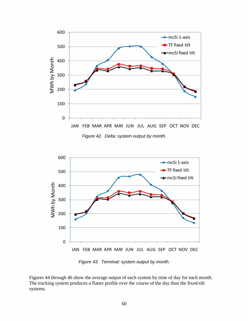
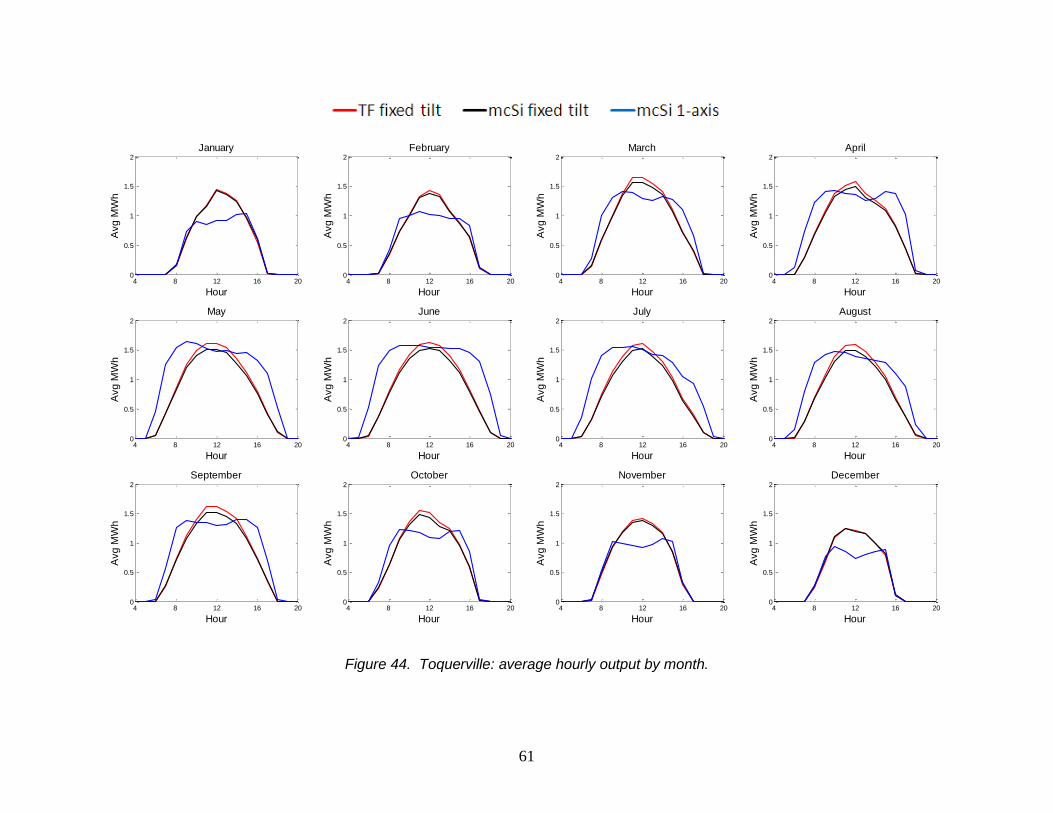
Figures 41 through 43 summarize system performance for each location as a function of time of
year. The thin-film systems have slightly higher output during the summer months than the
fixed-tilt multicrystalline system because of their lower temperature coefficient. Because the
tracking systems are flat and track the sun from east to west, they produce their highest
performance in the summer when the sun is higher in the sky.
Figure 41. Toquerville: system output by month.
0
100
200
300
400
500
600
JAN FEB MAR APR MAY JUN JUL AUG SEP OCT NOV DEC
MW
h b
y M
on
th
mcSi 1-axis
TF fixed tilt
mcSi fixed tilt
60
Figure 42. Delta: system output by month.
Figure 43. Terminal: system output by month.
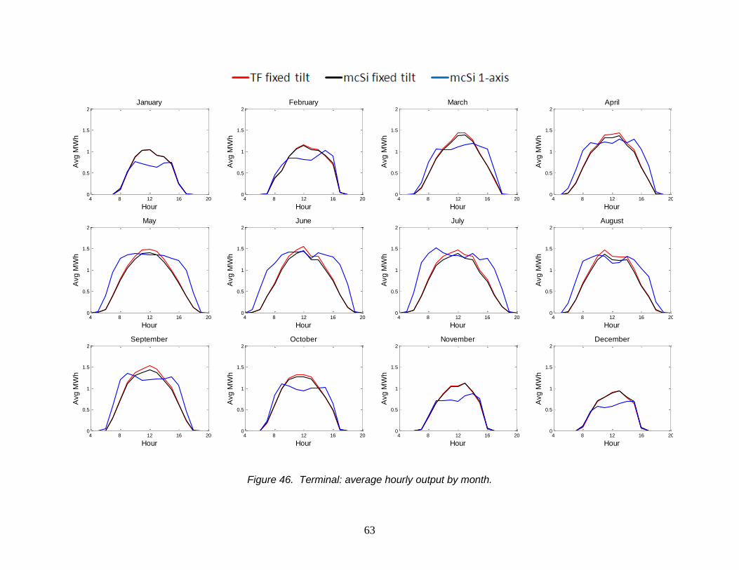
Figures 44 through 46 show the average output of each system by time of day for each month.
The tracking system produces a flatter profile over the course of the day than the fixed-tilt
systems.
0
100
200
300
400
500
600
JAN FEB MAR APR MAY JUN JUL AUG SEP OCT NOV DEC
MW
h b
y M
on
th
mcSi 1-axis
TF fixed tilt
mcSi fixed tilt
0
100
200
300
400
500
600
JAN FEB MAR APR MAY JUN JUL AUG SEP OCT NOV DEC
MW
h b
y M
on
th
mcSi 1-axis
TF fixed tilt
mcSi fixed tilt
61
Figure 44. Toquerville: average hourly output by month.
Toquerville
4 8 12 16 200
0.5
1
1.5
2
January
Hour
Avg
MW
h
4 8 12 16 200
0.5
1
1.5
2
February
Hour
Avg
MW
h
4 8 12 16 200
0.5
1
1.5
2
March
Hour
Avg
MW
h
4 8 12 16 200
0.5
1
1.5
2
April
Hour
Avg
MW
h
4 8 12 16 200
0.5
1
1.5
2
May
Hour
Avg
MW
h
4 8 12 16 200
0.5
1
1.5
2
June
Hour
Avg
MW
h
4 8 12 16 200
0.5
1
1.5
2
July
Hour
Avg
MW
h
4 8 12 16 200
0.5
1
1.5
2
August
Hour
Avg
MW
h
4 8 12 16 200
0.5
1
1.5
2
September
Hour
Avg
MW
h
4 8 12 16 200
0.5
1
1.5
2
October
Hour
Avg
MW
h
4 8 12 16 200
0.5
1
1.5
2
November
Hour
Avg
MW
h
4 8 12 16 200
0.5
1
1.5
2
December
Hour
Avg
MW
h

62
Figure 45. Delta: average hourly output by month.
Delta
4 8 12 16 200
0.5
1
1.5
2
January
Hour
Avg
MW
h
4 8 12 16 200
0.5
1
1.5
2
February
Hour
Avg
MW
h
4 8 12 16 200
0.5
1
1.5
2
March
Hour
Avg
MW
h
4 8 12 16 200
0.5
1
1.5
2
April
Hour
Avg
MW
h
4 8 12 16 200
0.5
1
1.5
2
May
Hour
Avg
MW
h
4 8 12 16 200
0.5
1
1.5
2
June
Hour
Avg
MW
h
4 8 12 16 200
0.5
1
1.5
2
July
Hour
Avg
MW
h
4 8 12 16 200
0.5
1
1.5
2
August
Hour
Avg
MW
h
4 8 12 16 200
0.5
1
1.5
2
September
Hour
Avg
MW
h
4 8 12 16 200
0.5
1
1.5
2
October
Hour
Avg
MW
h
4 8 12 16 200
0.5
1
1.5
2
November
Hour
Avg
MW
h
4 8 12 16 200
0.5
1
1.5
2
December
Hour
Avg
MW
h
63
Figure 46. Terminal: average hourly output by month.
Terminal
4 8 12 16 200
0.5
1
1.5
2
January
Hour
Avg
MW
h
4 8 12 16 200
0.5
1
1.5
2
February
Hour
Avg
MW
h
4 8 12 16 200
0.5
1
1.5
2
March
Hour
Avg
MW
h
4 8 12 16 200
0.5
1
1.5
2
April
Hour
Avg
MW
h
4 8 12 16 200
0.5
1
1.5
2
May
Hour
Avg
MW
h
4 8 12 16 200
0.5
1
1.5
2
June
Hour
Avg
MW
h
4 8 12 16 200
0.5
1
1.5
2
July
Hour
Avg
MW
h
4 8 12 16 200
0.5
1
1.5
2
August
Hour
Avg
MW
h
4 8 12 16 200
0.5
1
1.5
2
September
Hour
Avg
MW
h
4 8 12 16 200
0.5
1
1.5
2
October
Hour
Avg
MW
h
4 8 12 16 200
0.5
1
1.5
2
November
Hour
Avg
MW
h
4 8 12 16 200
0.5
1
1.5
2
December
Hour
Avg
MW
h
64
4 CONCLUSION
Despite the relatively high penetration levels, all feeders demonstrated acceptable electrical
performance results with a 2-MW PV system connected for the aspects studied, and the manner
in which they were studied. Additional study perspectives may reveal further impacts than those
discussed in this report. These may include protection impacts, flicker alternatives such as IEC
61000-4-15 standards, using local irradiance data to create more relative PV output behaviors for
each of the system types, and studying periods other than the two extremes demonstrated.
Based on the results of the electrical studies, the most extreme voltages found for each site under
all scenarios were, practically, as expected: highest voltage found during the Peak PV
Penetration period with PV and lowest voltage found during the Peak Load without PV. This
may be helpful in conducting interconnection studies using commercial simulation tools. Most, if
not all, of these tools allow for easy acquisition of extreme voltages for a snapshot power flow.
Although the Peak PV Penetration extreme periods found in this study may be difficult to
identify similarly for other feeders, it can be observed that they all occurred during the late
spring when temperatures are mild and loads are low, irradiance high, and on non-business days
(Sunday) around noon. Peak load periods are very commonly known by feeder across utilities, as
they are very useful in traditional planning.
Determining any reduction in demand because of PV integration was largely dependent on the
ability to perform time-series analysis, since it is highly dependent on the coincidence of load
and PV output. Further studies would be necessary to determine any consistencies found that
could lead to general recommendations when considering this without advanced modeling.
The presence of unity output PV reduces the measured feeder real power, while having no effect
on reactive power, and thus changing the perceived power factor. The actual load power factor is
unaffected. This may be an issue if any operations depend on power factor thresholds at the
feeder level.
Analyzing the effect of a PV system on LTC and line voltage regulator operations is also highly
dependent on the ability to perform time-series analysis, as well as model the source and
substation transformer. The operation of an LTC is dependent on the voltage drop across these
elements, which is dependent on the load current. The addition of all feeders connected to a
substation transformer gives a better indication of the actual operations to be expected. Time-
series analysis is also critical for incorporating the time delay aspect of the control settings. It
would be difficult to get an idea of this using commercial distribution tools.
The flicker analysis performed may show some similarities that can be valuable in approaching
this issue with commercial analysis tools. It can be observed that the largest voltage fluctuations
occurred practically independent of load level. It would be reasonable to conclude that a good
indication of worst-case voltage fluctuation could be observed during the peak load period. The
extreme method shown in this study would give a very conservative indication. Based on the PV
system output used in this study, and observations made from other data collections, analysis
using an assumption of 100-to-20 percent output, instead of the 100-to-0 percent output used
here, could be considered very near worst-case also. Once a worst-case magnitude is obtained, a

65
reasonable assumption can be made as to whether this fluctuation would occur frequently enough
to cause an irritation, according to IEEE Std 141-1993 [4] flicker limits. It is important to note
that there are alternative methods to analyzing potential flicker issues, such as defined by IEC
61000-4-15 [5] standards.

66
References
1. Ralph, M., A. Ellis, D. Borneo, G. Corey, and S. Baldwin, Transmission and Distribution
Deferment using PV and Energy Storage, (2010), Proceedings of the 35th
Photovoltaic
Specialists Conference, Honolulu, HI.
2. PVsyst computer application: http://www.pvsyst.com/, accessed on February 10, 2012
3. ANSI C84.1-1995, Electrical Power Systems and Equipment – Voltage Ratings (60 Hz),
1995, American National Standards Institute, 25 West 43rd
Street, 4th
Floor, New York,
NY 10036, USA
4. IEEE Std 141-1993, IEEE Recommended Practice for Electric Power Distribution for
Industrial Plants, pp. 93-94, 1994, The Institute of Electrical and Electronics Engineers,
Inc., 345 East 47th
Street, New York, NY 10017-2394, USA
5. IEC 61000-4-15, Electromagnetic compatibility (EMC) - Part 4-15: Testing and
measurement techniques - Flickermeter - Functional and design specifications, 2010,
International Electrotechnical Commission, 3, rue de Varembé, P.O. Box 131, CH - 1211
Geneva 20 - Switzerland
6. NREL Solar Prospector: http://maps.nrel.gov/node/10, accessed on February 10, 2012
7. Deline, Chris, Characterizing Shading Losses on Partially Shaded PV Systems, (2010),
Presentation at the PV Performance Modeling Workshop, Albuquerque, NM
(http://photovoltaics.sandia.gov/Pubs_2010/performance_modeling_workshop_cameron_
10/Deline_NREL_ShadeModeling.pdf), accessed on February 10, 2012

67
DISTRIBUTION
1 MS0899 RIM-Records Management 9532 (electronic copy)

68