
TAXATION OF SAVING - EMPIRICAL EVIDENCE
14.471 - Fall 2012
1

Why Are We Interested in the Tax Treatment of Saving?
1. Intertemporal Choices are an Important Potential Margin of Distortion (Optimal Capital Tax Literature)
2. Tax "Distribution Tables" Depend Critically on Tax Treatment of Capital Income (Highly Skewed)
3. Long-Standing Debate on Appropriate Base for Taxation: consumption, wages, income?
4. Policy Concern: High Saving Countries Tend to be High Growth Countries. Golden Rule: sf(k) = (n + 8)k in steady state, where s = saving rate. Since steady state consumption c = (1-s)f(k) = f(k) - (n + 8)k, it's straightforward to show that steady-state consumption per capita is maximized when f'(k) = (n + 8). Tax rate on saving may help to move k toward or away from this "golden rule".
5. Open Economy Issues to Remember. While Saving = Investment in Closed Economies, this equivalence breaks down in the open economy.
6. Two Key Policy Issues: (a) taxation of income from capital: how should saving be taxed? (b) design of retirement saving policy
2
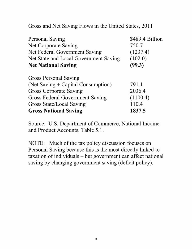
Gross and Net Saving Flows in the United States, 2011
Personal Saving $489.4 Billion Net Corporate Saving 750.7 Net Federal Government Saving (1237.4) Net State and Local Government Saving (102.0) Net National Saving (99.3)
Gross Personal Saving (Net Saving + Capital Consumption) 791.1 Gross Corporate Saving 2036.4 Gross Federal Government Saving (1100.4) Gross State/Local Saving 110.4 Gross National Saving 1837.5
Source: U.S. Department of Commerce, National Income and Product Accounts, Table 5.1.
NOTE: Much of the tax policy discussion focuses on Personal Saving because this is the most directly linked to taxation of individuals – but government can affect national saving by changing government saving (deficit policy).
3

Balance Sheet for the U.S. Household Sector, 2012:Q2 Assets $76.1
Trillion Real Estate 19.1 Other Tangible Assets 5.1 Financial Assets 51.9 Deposits 8.7 Taxable Bonds 3.0 Tax-Exempt Bonds 1.8 Corporate Stock & Mutual Fund Shares 14.3 Noncorporate Business Equity 7.7
Pension Fund Reserves (incl. 401(k) & IRA) 13.7 Other 2.7 Liabilities 13.5 Mortgages 9.6 Other 3.9 Net Worth 62.7 Source: Federal Reserve Board, Flow of Funds Accounts of the United States Second Quarter 2012, Table B.100.
Compare: Owners Equity/Household Real Estate: 2006: 56.5%; 2009: 39.6%; 2012 Q2: 43.1%. Household Net Worth/Disposable Income: 2006: 6.6; 2009: 5.1; 2012 Q2: 5.3.
4

� � � ��
Analyzing Consumption vs. Income Taxes in Rational Expectations OLG Models
Key Papers: Summers (1981 AER), Auerbach and Kotlikoff, Dynamic Fiscal Policy (1987), Altig, Auerbach, Kotlikoff, Smetters, Walliser (2001 AER).
Key Assumptions for Auerbach/Kotlikoff 1987:
• closed economy • no uncertainty, perfect foresight • market clearing in all periods, all markets • “households” live for 55 years, work for 45 years • adjustment costs for investment
Household Utility: 1
� � � 1� � 55 � �����1-
� �1-U =� 1
�� I(1+ �)-(t-1)�
� � ct���1- 1
��� +�l �
� 1�������� �-1 �
�� �
t�1- 1� � t=1 �
�� �
Household Budget Constraint:
55 t -1D = I I (1+ r ) [w e (1- l )- c ] e = "skill adjustment factor"s t t t t t
t=1 s=1
5

Production Function for Firms:
Investment Adjustment Costs:
C(It) = [1 + (b/2)(It /Kt)]* It
Government Budget Constraint:
Dt+1 = Dt + Gt - Tt + r Dt
or
Key Parameter Choices: • Elasticity of Labor Supply (Elasticity of Substitution
between c and l) • Intertemporal Elasticity of Substitution
6
t
t1 r 1
s Tt D r 10 1 s Gt
t 0 s 0 t 0 s 0
11111
1
11 11H
hthtt lky

Intertemporal Elasticity of Substitution (y)
Elasticity of Substitution between consumption & leisure (p)
Elasticity of Substitution in Production (c)
Steady State Efficiency Gain from Cons. Tax (% Lifetime Wealth)
Steady State Change in Real Wage (%) Cons. Tax
Wage Tax
Capital Income Tax
0.25 0.80 1.0 0.29% 6% 2% -13% 0.10 0.80 1.0 0.37 6 2 -8 0.50 0.80 1.0 0.28 6 3 -17 0.25 0.30 1.0 0.25 6 2 -12 0.25 1.50 1.0 0.36 5 2 -13 0.25 0.80 0.8 0.19 4 2 -16 0.25 0.80 1.25 0.45 8 2 -9
All policy experiments are relative to an income tax at an initial tax rate of 15%. Source: Auerbach and Kotlikoff (1987, Table 5.4).
7

8
© Cambridge University Press. All rights reserved. This content is excluded from ourCreative Commons license. For more information, see http://ocw.mit.edu/fairuse.

Role of Empirical Work in Studying Taxation and Household Saving
* Describe Stylized Facts about Household Saving Behavior
* Help Determine Which of Three Models (Lifecycle, Dynastic Altruism, Precautionary) is “Right”. (Are these distinct models? LCH can be augmented with precautionary demand for wealth or with bequest motives.)
* Calibrate Specific Models for Studying Behavioral Responses to Tax-Induced Changes in Rates of Return or Other Aspects of Saving Environment. Examples: Intertemporal Elasticity of Substitution (IES) Determines Distortion in Consumption Profile When Rate of Return Changes; Shape of “Marginal Utility of Bequest” Function Determines Response to an Estate Tax.
9

1. Background to Empirical Work: Saving Decisions Take Place in a Complex Institutional Environment
* In the “standard textbook model,” investors can earn rate of return r, borrow and lend at the same rate.
* In reality, investors face different borrowing and lending rates, both before and after tax; the tax treatment of income from saving and investing differs depending on the particular asset the individual is holding; saving can take place in a “tax deferred account” (like IRA) or in a traditional taxable setting
2. Margins of Distortion in Household Saving Behavior
* How Much to Save (traditional intertemporal choice problem that income tax affects)
* Asset Allocation: Which Assets to Hold, What Fraction of the Portfolio to Allocate to Each (relates to puzzle of limited stock ownership; stocks vs. bonds, tax-exempt bonds vs. taxable bonds)
* Asset Location: Which Assets to Hold in Taxable Accounts, which Assets to Hold in Tax-Deferred Accounts
* Asset Sale and Purchase Decisions: Trading Decision is affected by Capital Gains Taxation
* Leverage Decision: How Much to Borrow, and in What Form
10

3. Stylized Facts about Household Wealth Holdings
* Portfolios are Incomplete: Many Households Hold only a Small Set of Possible Assets (Fixed Income Assets, Stocks, Owner-Occupied Real Estate, Tax-Exempt Bonds) Data from 2007 SCF: 91% of Families have transaction accounts, 20.7% hold stocks outside retirement accounts, 12.7% hold CDs, 49.7% hold Retirement Accounts, 93.8% have some financial assets, 86% own at least one car; 70% own a house
* Wealth Holdings are Very Concentrated/Distribution is Very Skewed: Top 1% about 50% of Financial Wealth, 40% of Net Worth Including Tangible Assets; Top 10% about 80% of Financial, 70% of Total. 2007 Family Net Worth (Survey of Consumer Finances): Median $120,300 but Mean $556,300.
* Many Households Have Virtually No Wealth (about 30% negative net financial wealth, 20% negative net worth)
* Limited Liquid Wealth: Hall (2011 Presidential Address: 58% of Earnings to 74% of Households with Less than Two Months of Earnings in Liquid Form)
* Portfolios of High-Net-Worth Households Are Different from Those of Low-Net-Worth Households (Less Reliance on Owner-Occupied Housing, Greater Holdings of Equity, Great Exposure to “Alternative” Asset Classes, Business Equity > 1/3 of wealth for top 1%). House Value
11

/ Total Assets: Bottom quintile 47%, next 52%, next 48%, next 45%, percentiles 80-90 45%, percentiles 90-100, 20%.
* Wealth-Age Profile is Upward Sloping through ages in the early 60s. Evidence of draw-down of assets in retirement is much weaker.
* Inherited Wealth Appears to Account for a Substantial Fraction of Household Wealth (latest evidence, Gale and Scholz JEP 1994, suggests about half of existing wealth due to bequests).
5. Different Tax Rules for Different Asset Categories
* Saving Accounts, CDs, Treasury bonds: Interest income, taxed at ordinary tax rate
* Stocks: Dividends (taxed at dividend tax rate, now 15%) and Capital Gains (taxed at realization at capital gains tax rate – now 15% if Long Term (> 1 year))
* Tax-Exempt Bonds: Untaxed * Equity Mutual Funds: Dividends taxed like stocks;
capital gains taxed as realized by the fund (not the investor) * Tax-Deferred Accounts (IRAs, 401(k)s): No
taxation on returns until funds are withdrawn from the account, then taxed as ordinary income)
* Note that tax differences may facilitate tax avoidance ("Stiglitz Strategies" for capital gains)
12

Taxation and Personal Saving: Empirical Evidence
Broad Outline: - Standard intertemporal model and associated empirical results - Additional features: precautionary saving and behavioral
issues
Policy Issues: consumption vs. income taxation, retirement saving policy
Traditional Theory Offers Ambiguous Prediction about Impact of a Tax-Induced Decline in the real After-Tax Return on Level of Current Consumption:
– Substitution Effect Makes Future Consumption More Expensive So Increases Current C
– Income Effect (two period model with endowment given in first period) Household is Poorer (rise in price of future C) so Current C Should Decline
– “Human Wealth Effect” – PDV of Future Labor Income or Other Receipts Rises Which can Increase Current Consumption
Prior to late 1970s very little empirical evidence that changes in rates of return affected consumption (even though C(Y, W, r) was a standard in Keynesian macro models).
13
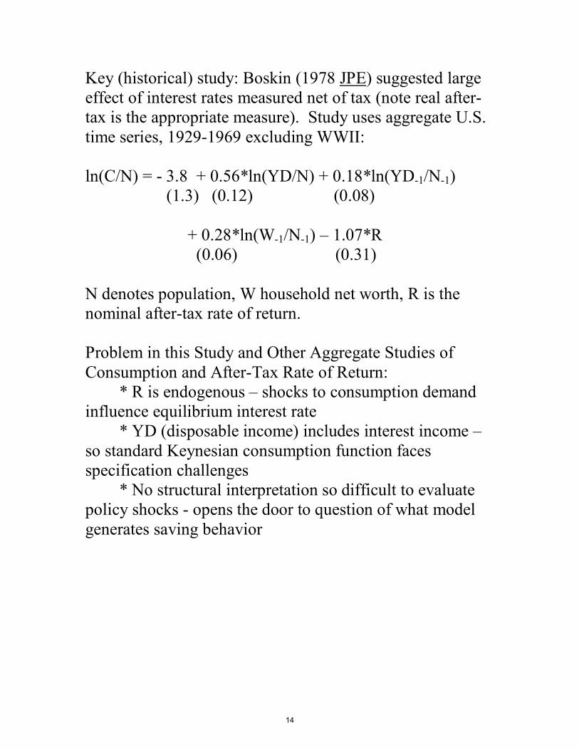
Key (historical) study: Boskin (1978 JPE) suggested large effect of interest rates measured net of tax (note real aftertax is the appropriate measure). Study uses aggregate U.S. time series, 1929-1969 excluding WWII:
ln(C/N) = - 3.8 + 0.56*ln(YD/N) + 0.18*ln(YD-1/N-1) (1.3) (0.12) (0.08)
+ 0.28*ln(W-1/N-1) – 1.07*R (0.06) (0.31)
N denotes population, W household net worth, R is the nominal after-tax rate of return.
Problem in this Study and Other Aggregate Studies of Consumption and After-Tax Rate of Return:
* R is endogenous – shocks to consumption demand influence equilibrium interest rate
* YD (disposable income) includes interest income – so standard Keynesian consumption function faces specification challenges
* No structural interpretation so difficult to evaluate policy shocks - opens the door to question of what model generates saving behavior
14

Tests of Competing Models: Altruism & Intergenerational Transfers
Altruism with operative transfers implies very strong predictions. Each parent cares about utility of children. Let U(C) denote the utility flow from own consumption. For parents:
Vp = U(Cp) + e��(�k)
Cp and Ck are consumption of the parent and child, respectively. Let Yp and Yk denote income of the parent and child and T a transfer from the parent to the child. Assume T > 0. The parent chooses T to maximize:
Vp = U(Yp - T) + e*U(Yk + T)
If the income of the child is fixed (Yk), the first order condition for the optimal transfer sets
U’(Cp�) = e��’(Ck*)
Note that all of T*, Cp*, and Ck* depend on the sum Yp + Yk but not on the values of the two components (provided the values of Yp and Yk are such that T* > 0.) By definition the optimal transfer is equal to:
T* = Ck* - Yk.
15

Now consider an income shock that raises parental income by � and reduces child income by �. If T� was optimal at the initial income levels, then T* + � will be optimal in the new setting – the allocation of consumption between parent and child will not depend in this case on the division of income between parent and child. This is a testable prediction – the consumption patterns within a dynasty should not depend on where in the dynasty the income accrues.
Altonji, Hayashi, and Kotlikoff (AER December 1992) use food consumption in the PSID to test this hypothesis.
16

17
© American Economic Association. All rights reserved. This content is excluded from ourCreative Commons license. For more information, see http://ocw.mit.edu/fairuse.

1993
1995
1995
1998
1998
2000
2000
2002
2002
2004
2004
2006
Testing the Lifecycle Model: Do Households Draw Down Assets in Old Age?
Simple Lifecycle Model with No Bequest Motive, No Uninsured Late-Life Medical Expenses, and Stochastic Life-Length Predicts Full Annuitization of Wealth at Retirement. Private Annuitization Rates are Very Low.
What About Patterns of Drawing Down Assets Held in Retirement?
Figure 3-1. Mean total assets for AHEAD persons age 70 to 80 in 1993, trimmed
0
100,000
200,000
300,000
400,000
500,000
600,000
dolla
rs
year
2�� 2������ 1��
Source: Poterba/Venti/Wise, “Family Status Transitions, Latent Health, and Post-Retirement Evolution of Assets,” NBER WP 15789, 2010.
18

Michael Hurd (AER 1987): Does one find different rates of decumulation by those with and without children? No – he argues this supports the LCH. Data from Retirement History Survey (RHS – 1969-79) not Health and Retirement Survey (1992 -). Findings from RHS:
Marital Status With Children Without Children Couples -17% -2% Singles -38% -33% All -28% -24%
Why the different findings with different surveys (AHEAD vs. RHS for example)?
• For households with wealth holdings, rates of return can be a key determinant of wealth trajectory (most households “drew down” in 2008).
• Changing generosity of annuitized programs – Social Security, Medicare, private pensions.
• Draw-down may be done sharply around significant life events (medical or nursing home needs).
19

Estimating the Intertemporal Elasticity of Substitution
Recall that in a two-period lifecycle model, a la King or Atkinson-Sandmo, the optimal tax burden on capital and the efficiency cost of taxing capital depend on the elasticity of second-period consumption with respect to the after-tax rate of return.
The most common parametric form for the utility function is power utility: U(C) = Cy/y. If the consumer is maximizing
v = L (1+8)-t Cty/y
and if the after-tax rate of return is (1-T)r then the "Euler Equation” that can be derived from the first order conditions for optimal choice of C0 and C1 is:
(C1/C0)(y-1) = (1+8)/(1+(1-T)r).
Taking logs of this expression yields the most common estimating equation in the IES literature:
ln(C1/C0) = (1/(y-1))� ln(1+8) - (1/(y-1))*ln(1+(1-T)r).
The parameter (-1/(y-1)) is the IES (the percentage change in the consumption growth rate from a percentage change in the after-tax price of consumption in period 1 versus period 0). Note this is also -1/RRA, where RRA is the coefficient of relative risk aversion. (note link to equity premium puzzle).
20
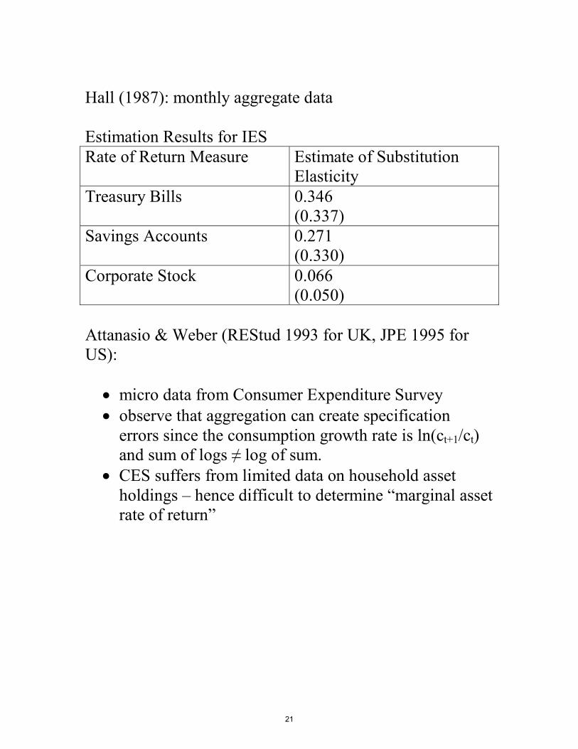
Hall (1987): monthly aggregate data
Estimation Results for IES Rate of Return Measure Estimate of Substitution
Elasticity Treasury Bills 0.346
(0.337) Savings Accounts 0.271
(0.330) Corporate Stock 0.066
(0.050)
Attanasio & Weber (REStud 1993 for UK, JPE 1995 for US):
• micro data from Consumer Expenditure Survey • observe that aggregation can create specification
errors since the consumption growth rate is ln(ct+1/ct) and sum of logs i log of sum.
• CES suffers from limited data on household asset holdings – hence difficult to determine “marginal asset rate of return”
21

Attanasio & Weber (JPE Dec 1995)
22
© The University of Chicago Press. All rights reserved. This content is excluded from our Creative Commons license. For more information, see http://ocw.mit.edu/fairuse.

23
© The University of Chicago Press. All rights reserved. This content is excluded from ourCreative Commons license. For more information, see http://ocw.mit.edu/fairuse.

24
© The University of Chicago Press. All rights reserved. This content is excluded from ourCreative Commons license. For more information, see http://ocw.mit.edu/fairuse.
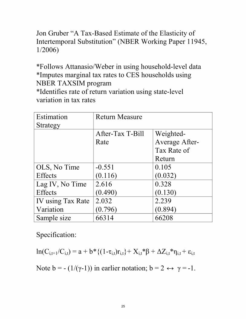
Jon Gruber “A Tax-Based Estimate of the Elasticity of Intertemporal Substitution” (NBER Working Paper 11945, 1/2006)
*Follows Attanasio/Weber in using household-level data *Imputes marginal tax rates to CES households using NBER TAXSIM program *Identifies rate of return variation using state-level variation in tax rates
Estimation Strategy
Return Measure
After-Tax T-Bill Rate
Weighted-Average After-Tax Rate of Return
OLS, No Time Effects
-0.551 (0.116)
0.105 (0.032)
Lag IV, No Time Effects
2.616 (0.490)
0.328 (0.130)
IV using Tax Rate Variation
2.032 (0.796)
2.239 (0.894)
Sample size 66314 66208
Specification:
25
ln(Ci,t+1/Ci,t) = a + b*{(1- i,t)ri,t}+ Xi,t* + Zi,t* i,t + i,t Note b = - -1)) in earlier notation; b = 2 -1.

Precautionary Saving Models
1. Risk of Late-Life Expenses (CBO Projections for 65year-olds in 2010)
* Any Nursing Home Use: 45% * One Year or Longer in a Nursing Home: 25% * Average Nursing Home Costs: $187/day for Semi-
Private Room, $209/day for Private Room
2. Hubbard/Skinner/Zeldes (JPE 1994) Model of Precautionary Saving Demand and Transfer Programs
Key Insight: Wealth-Tested Transfer Programs Provide Strong Disincentive for Low-Income Households to Save
Contributions: i) potential explanation for low levels of saving observed for many households; ii) investigation of how social insurance programs affect saving; iii) explicit modeling of uncertainty that may affect households
26

27
© The University of Chicago Press. All rights reserved. This content is excluded from ourCreative Commons license. For more information, see http://ocw.mit.edu/fairuse.

�
Households maximize v = L Dt (1+8)-t Cty/y
Dt = probability of survival to year t. At = assets in period t
At = At-1(1+r) + Et + TR(Et, Mt, At-1(1+r)) - Mt - Ct)
TR = max {0, Cfloor + Mt - At-1(1+r) - Et}
Cfloor is a consumption floor set by government transfer programs (Medicaid, Food Stamps, Public Housing)
28
© The University of Chicago Press. All rights reserved. This content is excluded from ourCreative Commons license. For more information, see http://ocw.mit.edu/fairuse.

Two stochastic shocks: Mt and Et. Key question: How persistent are the shocks.
Earnings Estimation: PSID
ln Ei,t = Xi,t*� + ui,t + �i,t
Estimate of pu: 0.955 < HS degree; 0.946 HS or HS+; 0.955 College +
Medical Expenditure Shock Estimation: NMES
ln Mi,t = Xi,t*� + vi,t + �i,t
vi,t = pv*vi,t-1 + ei,t
Estimate of pv: 0.901
Solution Algorithm: Find optimal Ct(Mt, Et, At-1, age, Cfloor). Solve by discretizing the range of possible values for {Mt, Et, age, At-1}. They consider 9 x 9 x 80 x 61 (=395,280 node) grid.
29
ui,t = u*ui,t-1 + i,t

30
© The University of Chicago Press. All rights reserved. This content is excluded from ourCreative Commons license. For more information, see http://ocw.mit.edu/fairuse.

Key Questions about Tax-Deferred Accounts
1. How do these accounts work? How important are they? Do they transform the income tax into a consumption tax for many households? (“hybrid tax”)
2. Does the availability of these accounts raise personal saving? Does it raise national saving? (Substitution is the key question)
3. How does the structure of these accounts affect saving decisions?
4. Are these accounts an adequate way to prepare for retirement?
The U.S. Institutional Setting
Saving through a Taxable Account Three relevant tax rates: T0 while earning, T1 while earning investment returns, T2 when withdrawing assets to finance consumption. Earn $1 and pay taxes on these earnings at rate T0
Earn rate of return (1-T1)r while saving No additional taxes when spend account proceeds Value of account (feasible consumption) after time T:
= (1-T0)*e(1-T1)rTVtaxable,T
Saving with a “Traditional” Individual Retirement Account (IRA) or 401(k) Plan Contribute before tax dollars
Earn rate of return r while saving Taxed at rate T2 when draw on funds for consumption
31

Value of account (feasible consumption) after time T:
VIRA,T = (1-T2)*erT
“Roth” IRA or 401(k) Pay taxes on period 0 earnings at rate T0 Contribute after tax dollars Earn rate of return r while saving No tax when draw on funds for consumption Value of account (=feasible consumption) at time T:
VRoth IRA,T = (1-T0)*erT
“Nondeductible” IRA (available when above income threshold for traditional deductible IRA)
Pay taxes on period 0 earnings at rate T0 Contribute after tax dollars Earn rate of return r while saving Taxed on difference between final balance and
contribution amount when draw on funds for consumption Value of account (=feasible consumption) in period T:
VNon-deductible IRA,T = (1-T0)*erT - T2[(1-T0)*erT - (1-T0)]
Accumulation Value: Traditional & Tax-Deferred Saving All Calculations Assume r=.06, constant T = 0.33 Account Type 10 Years 30 Years 50 Years Taxable 1.00 2.22 4.95 Deductible or Roth IRA 1.22 4.05 13.46 Non-Deductible IRA 1.04 2.93 9.24
32

Nomenclature for types of tax deferred accounts:
“EET” = “exempt, exempt, taxable” (traditional IRA) “TEE” = “taxable, exempt, exempt” (Roth IRA)
Institutional Details: U.S. Tax-Deferred Accounts
• Traditional “Deductible” IRA - Fully deductible contributions for incomes below
$53K (single), $85K (married joint) in 2009 - Partial Phase-out of deductibility (53-63K, 85
105K) - No tax on income accruing within IRA account - Fully taxable as ordinary income when
withdrawn - “Penalty Tax” of 10% if withdrawn before 59 ½ - Contribution limit: $5000 plus $1000 if over 50
(“catch up contribution”) - Required Minimum Distributions (RMDs) for
Account-holders over 70 ½ - Balance from a pension account can be “rolled
over” to an IRA when retire or leave employment - Can be bequeathed on favorable terms
33

• Roth IRA - No deduction for contributions - $5000 (+1000) contribution limit but in after tax
dollars (so like contribution $5000/(1-T0) dollars to a regular IRA)
- No taxation on withdrawals - No restrictions on withdrawals while contributor
is alive; RMDs apply after death
• 401(k) plans - Employer Sponsored Plans – key difference from
IRAs - Tax-deductible contributions (although there are
now Roth-401(k) variants at some firms) - Plans often include employer match so value at
withdrawal is V401(k),T = (1+m)*(1-TT)*erT where m = employer match rate
- Withdrawal rules similar to IRAs; RMDs after age 70 ½
- Contribution limits much higher than IRAs: $15,500 in 2009 plus $5000 catch-up if over 50
- No phase-outs with income - “Hardship withdrawals” if need assets while still
working; also loan provisions
Roll-over Opportunity: Income < $100K can convert Regular IRA to Roth IRA (note special 2010 provision: no limit on income for conversion)
34

Operation of 401(k)s and IRAs in U.S. * 1980: Roughly 75% of Pension Contributions in the
U.S. to Defined Benefit Plans * 2005: 73% of Pension Contributions to Defined
Contribution (401(k), 403(b)) Style Plans * DC Plan and IRA Assets in 2006: $8.3T ($16.4T in
Total Retirement Assets) * Future Retirees will Have Lifetime Exposure to
401(k)s (contrast with partial career exposure for current retirees)
* Potential to Accumulate Retirement Wealth: Consider Married Couple Contributing 8% of Salary for 30 Years, with 50/50 allocation and historical (pre-2008) equity returns, Median Balance at 65 for Median Earner: $468,000; 25th Percentile: $289,000; 75th Percentile $706,000
Actual 401(k) Balances for Various Years, SIPP Data Year Mean Median 1999 $66,660 $24,844 2003 $80,592 $43,127 2007 $137,430 $76,946
35

Participation and Eligibility in 401(k) Plans
36

Explain Structure of Defined Contribution and Defined Benefit Plans • Nature of Plans – Liabilities on Employers, Assets of
Workers • History of ERISA, PBGC Guarantees • Effects of Changing Stock Prices, Interest Rates on
Value of Assets and Liabilities in DB Plans • DB Plans Today (2009) Still Have Substantial Assets
but Contributions are Primarily DC
Effect of IRA & 401(k) Eligibility on Wealth Build-up
Earliest Studies of IRAs
• Discovered that Many Households Had Very Little Financial Wealth So Little Opportunity for Substitution
• 1986 SIPP Data (Venti & Wise): Contributors with IRA Assets of $7000 (median) have Non-IRA assets of $13,500; Non-Contributors Medial Non-IRA Financial Assets of $1000.
• Conflicting Evidence on IRAs (but little cross-sectional variation in eligibility for IRAs)
• Emphasize Difference Between Limit Contributors and Those Contributing Less than the Limit Amount
37

�
The 401(k) “Eligibility Experiment” • Since firms choose whether to offer 401(k) plans,
eligibility varies across households • What explains decision to offer 401(k)?
- Historical firm provision of profit-sharing plan - Median voter outcome reflecting preferences of
workers at the firm - Do firms with 401(k)s reduce availability of other
benefits? - Firm age, composition of workforce - younger
firms, more 401(k)s - Worker screening device: does desire to work at a
401(k)-employer signal “low discount rate” worker?
• Exogeneity of 401(k) eligibility: not a randomized trial, but not like universal-eligibility IRAs
• Participation Conditional on Eligibility: 36% in bottom decile, 65% at Median, 85% at top decile
Basic Specification (Poterba/Venti/Wise JPubE 1995 and subsequent studies) on repeated cross-sections with varying 401(k) eligibility
Aa,i = �a + Xi*� a + Ei*ya + ua,i
Allow for a and ya (already asset-specific) to vary by income of the household head. Thus the “eligibility effects” associated with Ei are different for high and low incomes.
38
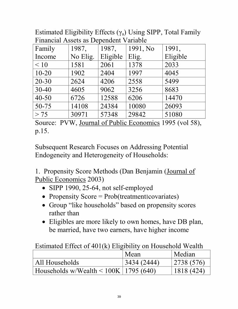
Estimated Eligibility Effects (ya) Using SIPP, Total Family Financial Assets as Dependent Variable Family Income
1987, No Elig.
1987, Eligible
1991, No Elig.
1991, Eligible
< 10 1581 2061 1378 2033 10-20 1902 2404 1997 4045 20-30 2624 4206 2558 5499 30-40 4605 9062 3256 8683 40-50 6726 12588 6206 14470 50-75 14108 24384 10080 26093 > 75 30971 57348 29842 51080 Source: PVW, Journal of Public Economics 1995 (vol 58), p.15.
Subsequent Research Focuses on Addressing Potential Endogeneity and Heterogeneity of Households:
1. Propensity Score Methods (Dan Benjamin (Journal of Public Economics 2003) • SIPP 1990, 25-64, not self-employed • Propensity Score = Prob(treatmentIcovariates) • Group “like households” based on propensity scores
rather than • Eligibles are more likely to own homes, have DB plan,
be married, have two earners, have higher income
Estimated Effect of 401(k) Eligibility on Household Wealth Mean Median All Households 3434 (2444) 2738 (576) Households w/Wealth < 100K 1795 (640) 1818 (424)
39

2. Quantile IV Estimation: Chernozhukov-Hansen (Review of Economics and Statistics, 2004) • Instrument for 401(k) Participation Using 401(k)
Eligibility • Allow Flexible Effects at Different Income Levels • Instruments for 401(k) Participation Using Eligibility • Cannot Reject Zero Effect of 401(k) Participation at
Lowest Income Levels, But Positive Effect of Participation at Higher Income Levels
• Evidence of Heterogeneity within Most Income Groups (but not highest)
Heterogeneity in Saving Effects: Larger Impact on Total Financial Assets for Low- and Moderate-Income Households, Still an Effect on Taxable vs. Tax-Deferred Asset Mix for High-Income Households
40

Margins on Which 401(k) or IRA Accumulation Might Crowd Out Other Wealth:
• Non-IRA, Non-401(k) Financial Assets • Other Pension Assets (Defined Benefit Plans) • Housing Equity (Borrowing Against Home to Fund
401(k) Plan)
Growth in 401(k) Asset Holdings Prospectively 2020 Retirement
Cohort 2040 Retirement Cohort
Historical Equity Return
Historical -300 bp Equity Return
Historical Equity Return
Historical – 300bp Equity Return
Lowest Decile
366 335 3688 2072
4th Decile 57614 46223 274958 172671 7th Decile 300917 230322 822220 484933 Highest 577632 454171 1242580 785150 Source: Poterba/Venti/Wise, “Rise of 401(k) Plans, Lifetime Earnings, & Wealth at Retirement,” NBER 2007.
Variation in 401(k) Accumulation: Sources of Heterogeneity • Contribution Rate • Match Rate • Earnings Trajectory • Returns While Accumulating • Date of Retirement
41

Variance in 401(k) Wealth at Retirement: HS and/or Some College Education, Normalized to Age 63/4 from Health and Retirement Survey 20th Percentile 0 40th Percentile 8000 Median 20400 60th Percentile 40300 80th Percentile 118900 Mean 83100 Source: Poterba/Rauh/Venti/Wise, “DC Plans, DB Plans, and the Accumulation of Retirement Wealth,” NBER WP 12597 (2006).
Relative Variance of DB and DC Plans: Both Have Substantial Variation (Samwick and Skinner, AER 2004).
Explaining the Level of 401(k) Contributions: Variables with Some Predictive Power • Financial Sophistication of Participant (Education as
Proxy) • Employer Match • “Behavioral” Factors
42

Defaults and 401(k) Behavior: Madrian-Shea QJE 2001. • Firm that shifted from “opt-in” to “opt-out” structure
of 401(k) plan. No changes to budget constraint facing employees.
• Participation Rate in 401(k) Before Opt-Out Plan: 57% at start of employment, 64% after 3-5 years, 83% for 20+ year employees
• Participation Rate After Opt-Out: 86% for new employees same tenure mix
• Why is this finding so important: Saving is a first-order decision for households (compare “book of the month club”) and it appears to be sensitive to framing and other considerations
Other Issues in Behavioral Economics • Failure of Households to Take Advantage of Match
Rates Even When Can Withdraw Immediately • Small Number of Rebalancing Transactions for Most
Households (Samuelson/Zeckhauser: Median Number of Rebalancing Transactions is ZERO at TIAA-CREF)
• Important Social Learning Effects (Duflo/Saez QJE: study librarians and their decisions with regard to 401(k) plan – if existing workers in “social group” contribute more, new workers do, too)
43

Designing “Opt-Out Policies” and Other Default Programs • Thaler Save More Tomorrow (SMART) plan • Default Options for Asset Allocation – Safe or
Exposed to Equities? • Challenges for Asset Allocation: Too Safe Yields too
Low a Return to Build Retirement Wealth, Too Risky Raises Risk of Losing Most Saving on Eve of Retirement
• How to Select Default Contribution Rate and Asset Allocation? Do Potential Participants Assume the Designated Allocation has been deemed “Optimal” by Someone?
• Critical Question: How to do Welfare Calculations when Individual Behavior does not follow neoclassical economic principles?
Effects of an “X% of Salary” Default Rule: • Some who would not contribute at all now contribute
X% • Some who would have contributed less than (more
than) X% now contribute X% • Some who would have made different asset
allocations now choose the default allocation • Welfare calculation will depend on elasticities of
participation, contribution level with respect to default, and on distribution of individuals pre-default across different contribution levels
44

Changing Evolution of Default Policies • Initially Money Market Funds (no risk for employer –
can’t lose money) • Now “Target Date Funds” that focus on automatic
age-related shifts in equity exposure • Key Role of “Safe Harbor” Provisions in Allowing
Employers to Offer Default Allocations that Involve Some Risk
Are IRAs & 401(k)s Generating Adequate Retirement Security? • “Replacement Rate” Calculation (Munnell, Webb,
Golub-Sass 2009 – Boston College “National Retirement Risk Index): 43% of Households Unable to Maintain Pre-Retirement Standard of Living in Retirement
• Comparison of Actual with “Model-Based” Wealth Accumulation (Scholz, Seshadri, & Khitatrakun, JPE 2006)
Earnings Decile % Households Below Optimal Wealth Target
Median Deficit (conditional on deficit)
Lowest 30.4% $2481 4th 19.4% $4730 7th 9.9% $11379 Top 5.4% $25855 All Households 15.6% $5260
Key Difference: Treatment of Housing Equity
45

MIT OpenCourseWarehttp://ocw.mit.edu
14.471 Public Economics IFall 2012
For information about citing these materials or our Terms of Use, visit: http://ocw.mit.edu/terms.


