Download - Supply Chain Management on Demand || Supply Chain Simulation

2 Supply Chain Simulation

Steve Buckley and Chae An

2.1 Introduction

Analysis, planning and control of a supply chain calls for a combination of spreadsheet, optimization and simulation models. Spreadsheet analysis is by far the most popular form of supply chain modeling due to its accessi-bility, ease of use and flexibility. However, spreadsheets are fairly limited in modeling power, with a few notable exceptions (Katircioglu et al. 2002). Optimization technology such as linear or mixed integer program-ming is a great way to solve well-defined mathematical problems such as supply network planning and inventory optimization (Ettl et al. 2000). But optimization models are rigidly structured and often based on simplifying assumptions to make the problem fit the mathematical format required by the underlying solver. Another issue that often limits the utility of optimi-zation is uncertainty. Uncertainty abounds in supply chains – for example in customer demand, lead times and supply availability. Although optimi-zation under uncertainty is a popular research topic, few commercial sup-ply chain optimization tools support uncertainty models.

Simulation is a popular alternative to optimization for supply chain analysis. Simulation models are not restricted by rigid mathematical struc-tures. Almost any supply chain issue can be coded as a simulation object with a set of parameterized behaviors. Individual components of a supply chain can be modeled separately and then combined into one large simula-tion model to represent the overall system. With simulation it is relatively easy to incorporate uncertainty, by generating random numbers for uncer-tain parameters during simulation runs. Multiple iterations are required to understand the results of uncertainty.

To be fair, it should be noted that simulation is an evaluative technique and does not automatically produce an optimal solution, unless simulation runs are controlled by an external search loop using an approach like De-sign of Experiments (Ermakov and Melas 1995). Moreover, supply chain

18 2 Supply Chain Simulation

simulations tend to be numerically intensive and sometimes take a long time to execute. Multiple iterations significantly increase the simulation runtime, as do external search loops such as Design of Experiments.

2.1.1 Comparison to Business Process Simulation

Off-the-shelf business process simulation tools have been readily available for about ten years. The popular commercial tools include ARIS (www.ids-scheer.com), Extend (www.imaginethatinc.com) and WBI Modeler (www.ibm.com/software/integration/wbimodeler). These simula-tors support general-purpose modeling of business activities but typically do not support detailed supply chain data structures such as demand fore-casts and bills of material; supply chain algorithms such as production planning, forecasting and replenishment; or supply chain policies like build-to-plan and build-to-order. Cycle times and resource usage are the primary outputs of business process simulations. While supply chain simu-lations are also concerned with these generic outputs, they are also focused on more specific metrics like inventory and customer service. There is a saying in supply chain circles that any mistake will lead to excess inven-tory and lower customer service. Calculating inventory and customer ser-vice requires detailed numerical data structures, algorithms and policies that are not found in general-purpose business process models.

If business process simulation tools were truly extensible, they would make it possible for supply chain developers to create and share libraries of supply chain data structures, algorithms and policies. In some cases, modelers have built upon business process simulation tools to analyze de-tailed supply chain issues, albeit for onetime analyses (Feigin et al. 1996).

2.2 Simulation Modeling Requirements

In this section, we discuss the modeling requirements necessary for accu-rately analyzing supply chain issues through simulation technology. These requirements are derived from a large number of supply chain modeling studies that researchers at IBM have performed during the past ten years.

2.2 Simulation Modeling Requirements 19

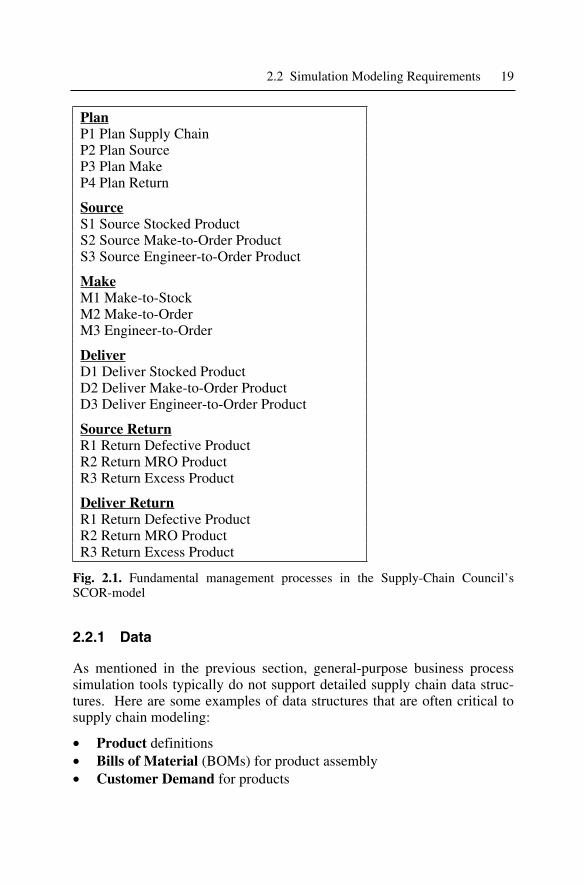
PlanP1 Plan Supply Chain P2 Plan Source P3 Plan Make P4 Plan Return

SourceS1 Source Stocked Product S2 Source Make-to-Order Product S3 Source Engineer-to-Order Product

MakeM1 Make-to-Stock M2 Make-to-Order M3 Engineer-to-Order

DeliverD1 Deliver Stocked Product D2 Deliver Make-to-Order Product D3 Deliver Engineer-to-Order Product

Source ReturnR1 Return Defective Product R2 Return MRO Product R3 Return Excess Product

Deliver ReturnR1 Return Defective Product R2 Return MRO Product R3 Return Excess Product

Fig. 2.1. Fundamental management processes in the Supply-Chain Council’s SCOR-model

2.2.1 Data

As mentioned in the previous section, general-purpose business process simulation tools typically do not support detailed supply chain data struc-tures. Here are some examples of data structures that are often critical to supply chain modeling:

• Product definitions• Bills of Material (BOMs) for product assembly • Customer Demand for products


• Customer Classes describing customer service requirements for dif-ferent types of users

• Demand Forecasts predicting customer demand over future time pe-riods

• Initial Inventory levels for products at a location • Storage Space definitions including storage size and associated costs • Reorder Points for maintaining stock levels • Lot Sizes for inventory replenishment • Supply Constraints limiting the number of products available from an

external supplier over a period of time • Locations of customers, distribution centers and manufacturing sites • Routes between locations and the transport time between them

2.2.2 Processes

The Supply-Chain Operations Reference (SCOR) model (Supply-Chain Council 2001) provides a starting point for building a simulation model of a supply chain (see Figure 2.1). The SCOR-model identifies five funda-mental supply chain management processes: Plan, Source, Make, Deliver and Return. We have found it extremely useful to model these fundamen-tal processes within the context of well-known supply chain business func-tions. Based on our experience, the following business functions are suffi-cient to model a variety of supply chain issues across many industries: Customer, Manufacturing, Distribution, Retail, Transportation, Inventory Planning, Forecasting and Supply Planning.

It is important to understand the scope of each fundamental process with respect to the business functions. The Plan process can apply to a single business function or to a set of business functions. For example, a Manu-facturing function may plan only its own activities based on inputs it re-ceives from other business functions in its supply chain. In other cases planning may be performed across business functions in an attempt to maximize overall supply chain value. For this reason three pure planning functions have been included in our list of business functions. The other fundamental processes – Source, Make, Deliver and Return – normally ap-ply to only a single business function.

For modeling purposes one can parameterize each business function in terms of the fundamental processes it executes. The following descriptions provide a high-level overview of this parameterization:

• Customer. This business function represents end customers that issue orders to other business functions. Customer functions execute the


fundamental processes Plan, Source and Return. Orders are generated on the basis of customer demand, which may be modeled as a se-quence of specific customer orders (possibly obtained from historical records) or as aggregated demand over a period of time (that must be randomly disaggregated during a simulation run). The Customer func-tion may also specify the desired due date, service level and priority for orders. Customer functions may send forecasts of future demand to other business functions.

• Manufacturing. This business function models assembly and main-tains raw material and finished goods inventory. Manufacturing exe-cutes the fundamental processes Plan, Source, Make, Deliver and Re-turn. Note that one Manufacturing function can supply another Manufacturing function, so there is no need to have a distinct function to model suppliers. A Manufacturing function makes use of modeled information such as the types of manufactured products, their manu-facturing cycle time, bills of material, manufacturing and replenish-ment policies for components and finished goods, reorder points, stor-age capacity, manufacturing resources, material handling resources and order queuing policies.

• Distribution. This business function models distribution centers and warehouses, including finished goods inventory and material handling. Distribution functions execute the fundamental processes Plan, Source, Deliver and Return. A Distribution model typically includes inventory replenishment policies, reorder points, storage capacity, material han-dling resources and order queuing policies.

• Retail. This business function models retail stores, including finished goods inventory and material handling. Retail stores execute the fun-damental processes Plan, Source, Deliver and Return. A Retail model typically includes inventory replenishment policies, safety stock poli-cies, reorder points, material handling resources, backroom storage ca-pacity and shelf space.

• Transportation. This business function models transportation types (e.g. trucks, planes, trains, boats), cycle time between shipping loca-tions, vehicle loading and transportation costs. Transportation exe-cutes the fundamental processes Plan, Deliver and Return. A Transpor-tation model typically includes order batching policies (by weight or volume), material handling resources and transportation resources.

• Inventory Planning. This business function models periodic setting of inventory target levels. Inventory Planning executes the fundamen-tal process Plan. This business function may link to an optimization program that computes recommended inventory levels based on de-


sired customer serviceability, product lead times and other considera-tions.

• Forecasting. This business function models product sales forecasts for future periods. Forecasting executes the fundamental process Plan. This business function may link to an optimization program.

• Supply Planning. This business function models bill-of-material ex-plosion and allocation of production and distribution resources to fore-casted demand under capacity and supply constraints. Supply Planning executes the fundamental process Plan. This business function may link to an optimization program.

In a supply chain it is important to distinguish between execution and planning processes. Execution processes are driven by plans and policies generated by planning processes. Both information and physical goods en-ter and leave execution processes. Planning processes deal only with in-formation, not physical goods. Three of the business functions listed above are pure planning functions: Forecasting, Inventory Planning and Supply Planning. The other business functions can have a mixture of execution and planning processes.

2.2.3 Entities

In a simulation model, the items that enter and leave business processes are often referred to as entities or artifacts. Here is a list of entities that are specific to supply chain processes:

• Request Orders represent customer or replenishment orders for physical goods. These entities carry order information from Customers to Manufacturing and Distribution functions and from Manufacturing and Distribution functions to other Manufacturing and Distribution functions.

• Filled Orders represent customer or replenishment orders for which physical goods have been provided. These entities carry order physical goods from Manufacturing and Distribution functions to Customer, Manufacturing and Distribution functions. Filled orders may pass through Transportation functions where aggregation and transport oc-curs.

• Shipments represent a group of Filled Orders in transport. These enti-ties carry Filled Orders from Transportation functions to Customer, Manufacturing and Distribution functions.

• Forecasts represent demand forecasts for customer and replenishment orders. These entities often carry demand forecast information from Forecasting functions to Supply Planning, Manufacturing and Distri-


bution functions. It is also possible for a Customer, Manufacturing, or Distribution function to have its own local forecasting process. If such a function shares its forecasts with other supply chain functions, it would do so by sending Forecast entities.

• Supply Plans represent production and procurement plans generated by a Supply Planning function, often based on forecast information. These entities usually carry information from Supply Planning func-tions to Distribution and Manufacturing functions.

2.2.4 Resources

The resource models provided by general-purpose business process simu-lators are often useful for supply chain simulation. Since cycle time and resource cost are key metrics in both business process and supply chain simulations, business process resource definitions can sometimes be reused for supply chain simulation. However, additional parameters and con-structs are often needed to model the following supply chain resources:

• Storage Resources model cost and capacity of space where Manufac-turing, Distribution and Transportation functions store physical goods.

• Material Handling Resources model cost and capacity of personnel and equipment used to move physical goods within Manufacturing, Distribution and Transportation functions.

• Manufacturing Resources model cost and capacity of personnel and equipment used to manufacture physical goods in Manufacturing func-tions.

• Transportation Resources model cost and capacity of vehicles such as trucks, trains and ships in Transportation functions.

2.2.5 Supply Chain Process Example

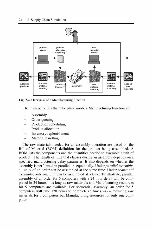
To illustrate a supply chain process, let us examine the Manufacturing function shown in Figure 2.2. A Manufacturing function assembles, stores and sells physical goods (products). A Manufacturing function can supply a Customer function, a Distribution function, or another Manufacturing function with products. It may require raw materials which can be ordered from a Distribution function or another Manufacturing function. Produc-tion schedules can be driven by Supply Plans received from Supply Plan-ning functions or by Request Orders.


Fig. 2.2. Overview of a Manufacturing function

The main activities that take place inside a Manufacturing function are:

− Assembly − Order queuing − Production scheduling − Product allocation− Inventory replenishment − Material handling

The raw materials needed for an assembly operation are based on the Bill of Material (BOM) definition for the product being assembled. A BOM lists the components and the quantities needed to assemble a unit of product. The length of time that elapses during an assembly depends on a specified manufacturing delay parameter. It also depends on whether the assembly is performed in parallel or sequentially. Under parallel assembly,all units of an order can be assembled at the same time. Under sequential assembly, only one unit can be assembled at a time. To illustrate, parallel assembly of an order for 5 computers with a 24 hour delay will be com-pleted in 24 hours – as long as raw materials and Manufacturing resources for 5 computers are available. For sequential assembly, an order for 5 computers will take 120 hours to complete (5 times 24) – requiring raw materials for 5 computers but Manufacturing resources for only one com-puter.


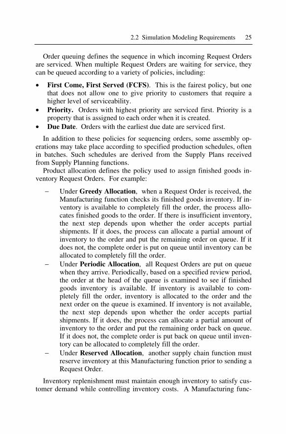
Order queuing defines the sequence in which incoming Request Orders are serviced. When multiple Request Orders are waiting for service, they can be queued according to a variety of policies, including:

• First Come, First Served (FCFS). This is the fairest policy, but one that does not allow one to give priority to customers that require a higher level of serviceability.

• Priority. Orders with highest priority are serviced first. Priority is a property that is assigned to each order when it is created.

• Due Date. Orders with the earliest due date are serviced first.

In addition to these policies for sequencing orders, some assembly op-erations may take place according to specified production schedules, often in batches. Such schedules are derived from the Supply Plans received from Supply Planning functions.

Product allocation defines the policy used to assign finished goods in-ventory Request Orders. For example:

− Under Greedy Allocation, when a Request Order is received, the Manufacturing function checks its finished goods inventory. If in-ventory is available to completely fill the order, the process allo-cates finished goods to the order. If there is insufficient inventory, the next step depends upon whether the order accepts partial shipments. If it does, the process can allocate a partial amount of inventory to the order and put the remaining order on queue. If it does not, the complete order is put on queue until inventory can be allocated to completely fill the order.

− Under Periodic Allocation, all Request Orders are put on queue when they arrive. Periodically, based on a specified review period, the order at the head of the queue is examined to see if finished goods inventory is available. If inventory is available to com-pletely fill the order, inventory is allocated to the order and the next order on the queue is examined. If inventory is not available, the next step depends upon whether the order accepts partial shipments. If it does, the process can allocate a partial amount of inventory to the order and put the remaining order back on queue. If it does not, the complete order is put back on queue until inven-tory can be allocated to completely fill the order.

− Under Reserved Allocation, another supply chain function must reserve inventory at this Manufacturing function prior to sending a Request Order.

Inventory replenishment must maintain enough inventory to satisfy cus-tomer demand while controlling inventory costs. A Manufacturing func-


tion maintains inventory in logical storage areas called buffers. Two types of buffers are maintained, input buffers for raw materials and output buff-ers for finished goods. A Manufacturing function sends out Request Or-ders to restock its input buffers. The assembly process transforms raw ma-terials in input buffers to finished goods in output buffers.

Raw materials can be either outsourced or insourced. Outsourced raw materials are ordered from another supply chain function. Insourced raw materials are manufactured at the same function where they are used.

A specified inventory replenishment policy determines when and how a Manufacturing function generates Request Orders to restock its buffers. Here are some examples of replenishment policies:

• Continuous Replenishment. The buffer is restocked whenever the inventory level in the buffer falls below a specified reorder point.

• Periodic Replenishment. The buffer is restocked periodically based on a specified review period, but only if the inventory level in the buffer is below its reorder point.

• Build-To-Order (BTO). This policy maintains minimum inventory by restocking a buffer only if a Request Order arrives and inventory is not available to fill the order.

• Build-To-Plan (BTP). Buffers are restocked according to Supply Plans received from Supply Planning functions.

In a Manufacturing function there are two types of material handling, inbound handling (dock-to-stock) and outbound handling (stock-to-dock). A Manufacturing process must model both the time and cost of material handling. Material handling cost can be modeled in a number of ways, for example:

− Cost per order − Cost per unit of weight − Cost per unit of volume − Cost per order per hour − Cost per unit of weight per hour − Cost per unit of volume per hour

Partial pallets are usually much more costly to handle than full pallets – this must also be captured in the cost model.

2.3 Strategic Uses of Supply Chain Simulation 27

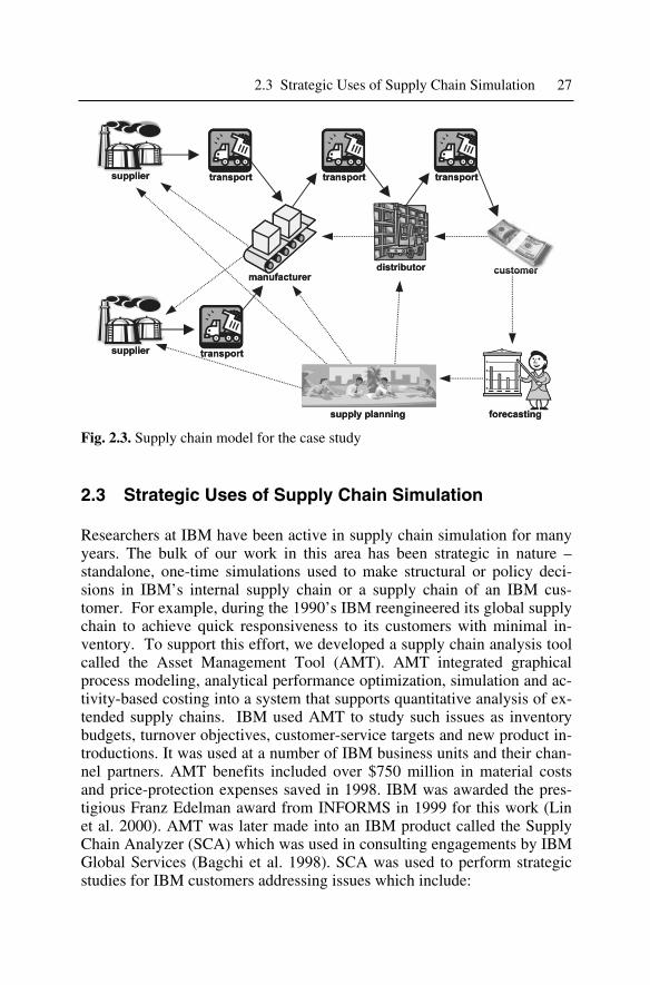
Fig. 2.3. Supply chain model for the case study

2.3 Strategic Uses of Supply Chain Simulation

Researchers at IBM have been active in supply chain simulation for many years. The bulk of our work in this area has been strategic in nature – standalone, one-time simulations used to make structural or policy deci-sions in IBM’s internal supply chain or a supply chain of an IBM cus-tomer. For example, during the 1990’s IBM reengineered its global supply chain to achieve quick responsiveness to its customers with minimal in-ventory. To support this effort, we developed a supply chain analysis tool called the Asset Management Tool (AMT). AMT integrated graphical process modeling, analytical performance optimization, simulation and ac-tivity-based costing into a system that supports quantitative analysis of ex-tended supply chains. IBM used AMT to study such issues as inventory budgets, turnover objectives, customer-service targets and new product in-troductions. It was used at a number of IBM business units and their chan-nel partners. AMT benefits included over $750 million in material costs and price-protection expenses saved in 1998. IBM was awarded the pres-tigious Franz Edelman award from INFORMS in 1999 for this work (Lin et al. 2000). AMT was later made into an IBM product called the Supply Chain Analyzer (SCA) which was used in consulting engagements by IBM Global Services (Bagchi et al. 1998). SCA was used to perform strategic studies for IBM customers addressing issues which include:


− Number and location of manufacturers and DC’s − Stocking level of each product at each site − Manufacturing and replenishment policies, e.g. Build-To-Plan

(BTP), Build-To-Order (BTO), Assemble-To-Order (ATO), Con-tinuous Replenishment (CR)

− Transportation policies − Supply planning policies − Lead times − Supplier performance − Demand variability

SCA was a standalone tool running on Windows with a user-friendly graphical interface. In order to provide model data to SCA one had to pre-pare a number of flat files in a specified format. In many cases this was a one-time manual process using query tools and spreadsheets. In some cases a bridge was constructed to SCA from enterprise databases.

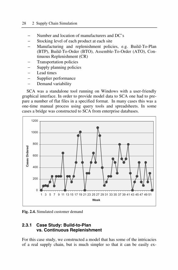
Fig. 2.4. Simulated customer demand

2.3.1 Case Study: Build-to-Plan vs. Continuous Replenishment

For this case study, we constructed a model that has some of the intricacies of a real supply chain, but is much simpler so that it can be easily ex-


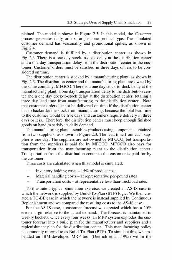
plained. The model is shown in Figure 2.3. In this model, the Customerprocess generates daily orders for just one product type. The simulated customer demand has seasonality and promotional spikes, as shown in Fig. 2.4.

Customer demand is fulfilled by a distribution center, as shown in Fig. 2.3. There is a one day stock-to-dock delay at the distribution center and a one day transportation delay from the distribution center to the cus-tomer. Customer orders must be satisfied in three days or less to be con-sidered on time.

The distribution center is stocked by a manufacturing plant, as shown in Fig. 2.3. The distribution center and the manufacturing plant are owned by the same company, MFGCO. There is a one day stock-to-dock delay at the manufacturing plant, a one day transportation delay to the distribution cen-ter and a one day dock-to-stock delay at the distribution center, totaling a three day lead time from manufacturing to the distribution center. Note that customer orders cannot be delivered on time if the distribution center has to backorder the stock from manufacturing, because the total lead time to the customer would be five days and customers require delivery in three days or less. Therefore, the distribution center must keep enough finished goods on hand to satisfy its daily demand.

The manufacturing plant assembles products using components obtained from two suppliers, as shown in Figure 2.3. The lead time from each sup-plier is one day. The suppliers are not owned by MFGCO, but transporta-tion from the suppliers is paid for by MFGCO. MFGCO also pays for transportation from the manufacturing plant to the distribution center. Transportation from the distribution center to the customer is paid for by the customer.

Three costs are calculated when this model is simulated:

− Inventory holding costs – 15% of product cost − Material handling costs – at representative per-pound rates − Transportation costs – at representative less-than-truckload rates

To illustrate a typical simulation exercise, we created an AS-IS case in which the network is supplied by Build-To-Plan (BTP) logic. We then cre-ated a TO-BE case in which the network is instead supplied by Continuous Replenishment and we compared the resulting costs to the AS-IS case.

For the AS-IS case, a customer forecast was created which has a 20% error margin relative to the actual demand. The forecast is maintained in weekly buckets. Once every four weeks, an MRP system explodes the cus-tomer forecast into a build plan for the manufacturer and suppliers and a replenishment plan for the distribution center. This manufacturing policy is commonly referred to as Build-To-Plan (BTP). To simulate this, we em-bedded an IBM-developed MRP tool (Dietrich et al. 1995) within the


simulator, labeled as Supply Planning in Figure 2.3. The build plans and replenishment plans are generated in weekly buckets. Note that in order for the distribution center to have enough on-hand stock to satisfy demand at the beginning of each week, manufacturing must build the forecasted de-mand the week before.

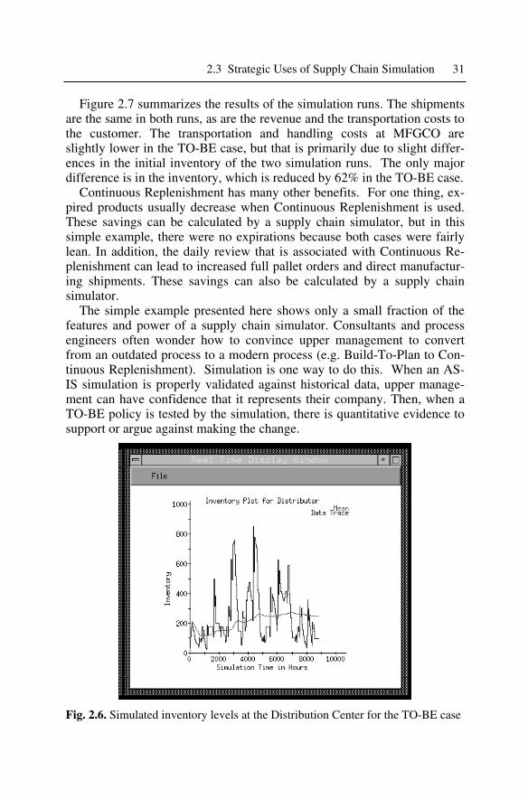
For the TO-BE case, the same customer forecast is used, but the inven-tory at each stocking location is reviewed daily. The forecast is used by an optimization program (Ettl et al. 2000) to set the reorder point at each stocking location each day. Whenever a reorder point exceeds the on-hand inventory, a replenishment order is sent out to make up the difference. This manufacturing policy is commonly referred to as Continuous Replenish-ment (CR).

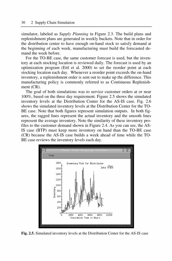
The goal of both simulations was to service customer orders at or near 100%, based on the three day requirement. Figure 2.5 shows the simulated inventory levels at the Distribution Center for the AS-IS case. Fig. 2.6 shows the simulated inventory levels at the Distribution Center for the TO-BE case. Note that both figures represent simulation outputs. In both fig-ures, the ragged lines represent the actual inventory and the smooth lines represent the average inventory. Note the similarity of these inventory pro-files to the customer demand shown in Figure 2.4. As you can see, the AS-IS case (BTP) must keep more inventory on hand than the TO-BE case (CR) because the AS-IS case builds a week ahead of time while the TO-BE case reviews the inventory levels each day.

Fig. 2.5. Simulated inventory levels at the Distribution Center for the AS-IS case


Figure 2.7 summarizes the results of the simulation runs. The shipments are the same in both runs, as are the revenue and the transportation costs to the customer. The transportation and handling costs at MFGCO are slightly lower in the TO-BE case, but that is primarily due to slight differ-ences in the initial inventory of the two simulation runs. The only major difference is in the inventory, which is reduced by 62% in the TO-BE case.

Continuous Replenishment has many other benefits. For one thing, ex-pired products usually decrease when Continuous Replenishment is used. These savings can be calculated by a supply chain simulator, but in this simple example, there were no expirations because both cases were fairly lean. In addition, the daily review that is associated with Continuous Re-plenishment can lead to increased full pallet orders and direct manufactur-ing shipments. These savings can also be calculated by a supply chain simulator.

The simple example presented here shows only a small fraction of the features and power of a supply chain simulator. Consultants and process engineers often wonder how to convince upper management to convert from an outdated process to a modern process (e.g. Build-To-Plan to Con-tinuous Replenishment). Simulation is one way to do this. When an AS-IS simulation is properly validated against historical data, upper manage-ment can have confidence that it represents their company. Then, when a TO-BE policy is tested by the simulation, there is quantitative evidence to support or argue against making the change.

Fig. 2.6. Simulated inventory levels at the Distribution Center for the TO-BE case


Fig. 2.7. Simulation results

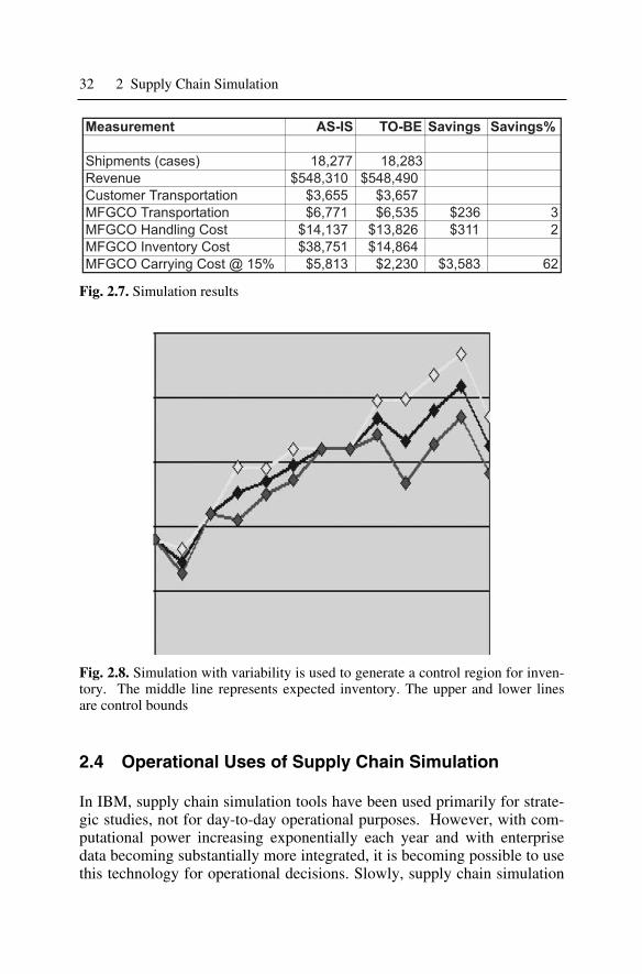
Fig. 2.8. Simulation with variability is used to generate a control region for inven-tory. The middle line represents expected inventory. The upper and lower lines are control bounds

2.4 Operational Uses of Supply Chain Simulation

In IBM, supply chain simulation tools have been used primarily for strate-gic studies, not for day-to-day operational purposes. However, with com-putational power increasing exponentially each year and with enterprise data becoming substantially more integrated, it is becoming possible to use this technology for operational decisions. Slowly, supply chain simulation

2.4 Operational Uses of Supply Chain Simulation 33

is spreading into the weekly and daily operations of enterprises. In the fu-ture, this transition will be made easier by the following advances:

− Simulation speed is increasing due to drastic improvements in computer technology coupled with careful design of simulation granularity.

− Simulation model data will become more integrated with enter-prise data. As Business Activity Monitoring (BAM) (April and Margulius 2002) and Business Performance Management (BPM) (www.ibm.com/ software/info/ topic/perform/resources.html) grow in popularity, simulation data will be more readily available in data warehouses, reducing the startup cost to create a simulation model.

− What-if simulation of alternatives will increasingly become part of decision-making processes.

− Business users of simulation technology will be presented with customized screen flows, not general-purpose simulation tooling. They may not even know that they are using a simulation tool.

− Simulation tools will be web-enabled. Business process manage-ment is shifting to the web and data is readily available on the Internet. Modern web portal technology supports customizable user interfaces.

The following scenarios illustrate the operational use of supply chain simulation:

• Process control. Simulation is used to predict the metrics of a process in an upcoming time period. The process is then tracked against the simulated results. For example, an IBM division uses simulation to predict their future product inventory levels at the beginning of each quarter (see Figure 2.8). Based on various uncertainties specified in the simulation, it is possible to generate lower and upper bounds for statis-tical control purposes. Actual inventory is then tracked against the control limits for early detection of unexpected situations.

• Decision support. When unexpected situations arise, there are often a number of alternative actions that can be taken. Simulation can be used to assess the benefit and risk of each potential response (Lin et al. 2002). For example, the potential responses to a late supplier delivery may include setting higher inventory targets, using a different supplier, and doing nothing. These alternatives can be simulated under the cur-rent business conditions to predict the profit, cost and serviceability for each alternative. From multiple runs these predictions can summarized in stochastic terms to estimate risk.


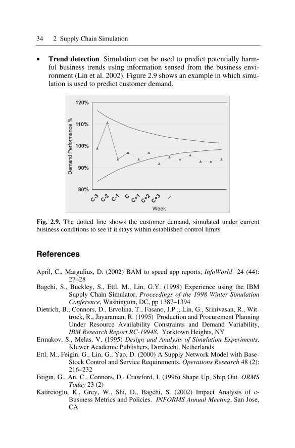
• Trend detection. Simulation can be used to predict potentially harm-ful business trends using information sensed from the business envi-ronment (Lin et al. 2002). Figure 2.9 shows an example in which simu-lation is used to predict customer demand.

Fig. 2.9. The dotted line shows the customer demand, simulated under current business conditions to see if it stays within established control limits

References

April, C., Margulius, D. (2002) BAM to speed app reports, InfoWorld 24 (44): 27–28

Bagchi, S., Buckley, S., Ettl, M., Lin, G.Y. (1998) Experience using the IBM Supply Chain Simulator, Proceedings of the 1998 Winter Simulation Conference, Washington, DC, pp 1387–1394

Dietrich, B., Connors, D., Ervolina, T., Fasano, J.P.,, Lin, G., Srinivasan, R., Wit-trock, R., Jayaraman, R. (1995) Production and Procurement Planning Under Resource Availability Constraints and Demand Variability, IBM Research Report RC-19948, Yorktown Heights, NY

Ermakov, S., Melas, V. (1995) Design and Analysis of Simulation Experiments.Kluwer Academic Publishers, Dordrecht, Netherlands

Ettl, M., Feigin, G., Lin, G., Yao, D. (2000) A Supply Network Model with Base-Stock Control and Service Requirements. Operations Research 48 (2): 216–232

Feigin, G., An, C., Connors, D., Crawford, I. (1996) Shape Up, Ship Out. ORMS Today 23 (2)

Katircioglu, K., Grey, W., Shi, D., Bagchi, S. (2002) Impact Analysis of e-Business Metrics and Policies. INFORMS Annual Meeting, San Jose, CA

2.4 Operational Uses of Supply Chain Simulation 35

Lin, G., Ettl, M., Buckley, S., Bagchi, S., Yao, D.D., Naccarato, B.L., Allan, R., Kim, K., Koenig, L. (2000) Extended-Enterprise Supply-Chain Man-agement at IBM Personal Systems Group and Other Divisions, Inter-faces 30 (1): 7–21

Lin, G., Buckley, S., Cao, H., Caswell, N., Ettl, M., Kapoor, S., Koenig, L., Katir-cioglu, K., Nigam, A., Ramachandran, B., Wang, K. (2002) The Sense-and-Respond Enterprise. OR/MS Today 29 (2): 34–39

Supply-Chain Council (2000) Supply-Chain Operations Reference-Model: Over-view of SCOR Version 5.0. Pittsburgh, PA: Supply-Chain Council Inc.

Download - Supply Chain Management on Demand || Supply Chain Simulation

Top Related