
Stormwater Best Management
Practices (BMP) Performance
Analysis December 2008 Prepared for: United States Environmental Protection Agency – Region 1 One Congress Street, Suite 1100 Boston, MA 02114 Prepared by: Tetra Tech, Inc. 10306 Eaton Place, Suite 340 Fairfax, VA 22030

BMP Performance Analysis
ii December 2008
Contents EXECUTIVE SUMMARYEXECUTIVE SUMMARYEXECUTIVE SUMMARYEXECUTIVE SUMMARY.................................................................................................................................................................................................................................................................................................................................................................................................................................................................................................................................... vivivivi
1. INTRODUCTION1. INTRODUCTION1. INTRODUCTION1. INTRODUCTION....................................................................................................................................................................................................................................................................................................................................................................................................................................................................................................................................................................7777
2. PRECIPITATION ANALYSIS2. PRECIPITATION ANALYSIS2. PRECIPITATION ANALYSIS2. PRECIPITATION ANALYSIS ................................................................................................................................................................................................................................................................................................................................................................................................................................................................................................9999
2.1. Data Collection and Review................................................................................................................... 9 2.2. Event Frequency Analysis ....................................................................................................................11
3. LAND ANALYSIS3. LAND ANALYSIS3. LAND ANALYSIS3. LAND ANALYSIS........................................................................................................................................................................................................................................................................................................................................................................................................................................................................................................................................................14141414
3.1. Land Representation for Pollutant Loading .......................................................................................14 3.2. Selection of Water Quality Model........................................................................................................16 3.3. Setup and Calibration of SWMM Water Quality Model......................................................................17
3.3.1. Water Quality Processes in SWMM.............................................................................................17 3.3.2. Setup and Calibration of SWMM.................................................................................................18
4. BMP ANALYSIS4. BMP ANALYSIS4. BMP ANALYSIS4. BMP ANALYSIS ............................................................................................................................................................................................................................................................................................................................................................................................................................................................................................................................................................20202020
4.1. BMPDSS Calibration and Testing........................................................................................................20 4.1.1. Overview of the Calibration Process ...........................................................................................20 4.1.2. BMPDSS Calibration Events ........................................................................................................22 4.1.3. BMPDSS calibration results.........................................................................................................23 4.1.4. BMPDSS Test Results ..................................................................................................................41 4.1.5. BMPDSS Calibration Summary....................................................................................................43
4.2. BMPDSS Representation.....................................................................................................................43 4.2.1. Infiltration System ........................................................................................................................43 4.2.2. Gravel Wetland .............................................................................................................................46 4.2.3. Bioretention Area .........................................................................................................................48 4.2.4. Porous Pavement .........................................................................................................................50 4.2.5. Water Quality Swales ...................................................................................................................52 4.2.6. Wet Retention Pond (Wet Basins) ...............................................................................................53 4.2.7. Extended Dry Detention (Dry Basins)..........................................................................................55
5. PERFORMANCE CURVE5. PERFORMANCE CURVE5. PERFORMANCE CURVE5. PERFORMANCE CURVE ........................................................................................................................................................................................................................................................................................................................................................................................................................................................................................................58585858
5.1. BMP Performance Curve and Application ..........................................................................................58 5.2. Example Application of BMP Performance Curve ..............................................................................60
5.2.1. Commercial Application ...............................................................................................................60 5.2.2. Low-Density Residential Application ...........................................................................................64
5.3. Assumptions and Limitations..............................................................................................................67
ACKNOWLEDGEMENTSACKNOWLEDGEMENTSACKNOWLEDGEMENTSACKNOWLEDGEMENTS ........................................................................................................................................................................................................................................................................................................................................................................................................................................................................................................................68686868
REFERENCESREFERENCESREFERENCESREFERENCES........................................................................................................................................................................................................................................................................................................................................................................................................................................................................................................................................................................................69696969
APPENDIX A: BACKGROUNDAPPENDIX A: BACKGROUNDAPPENDIX A: BACKGROUNDAPPENDIX A: BACKGROUND ON BMPDSS ON BMPDSS ON BMPDSS ON BMPDSS........................................................................................................................................................................................................................................................................................................................................................................................................71717171
A.1. Land Use Time Series ..........................................................................................................................71 A.2. BMPDSS................................................................................................................................................71
ArcGIS Interface.......................................................................................................................................72 BMP Simulation Module .........................................................................................................................72 Routing/Transport Module .....................................................................................................................73 Optimization Component ........................................................................................................................74 Post-processor.........................................................................................................................................74
A.3. BMP Model Representation.................................................................................................................75
BMP Performance Analysis
December 2008 iii
APPENDIX B: BMP RERFORMANCE CURVESAPPENDIX B: BMP RERFORMANCE CURVESAPPENDIX B: BMP RERFORMANCE CURVESAPPENDIX B: BMP RERFORMANCE CURVES........................................................................................................................................................................................................................................................................................................................................................................................78787878
BMP Performance Curve: Infiltration TrenchBMP Performance Curve: Infiltration TrenchBMP Performance Curve: Infiltration TrenchBMP Performance Curve: Infiltration Trench........................................................................................................................................................................................................................................................................................................................................................................................79797979
BMP Performance Curve: Infiltration BasinBMP Performance Curve: Infiltration BasinBMP Performance Curve: Infiltration BasinBMP Performance Curve: Infiltration Basin.................................................................................................................................................................................................................................................................................................................................................................................... 115115115115
BMP Performance Curve: Gravel WetlandBMP Performance Curve: Gravel WetlandBMP Performance Curve: Gravel WetlandBMP Performance Curve: Gravel Wetland............................................................................................................................................................................................................................................................................................................................................................................................ 152152152152
BMP Performance Curve: BioretentionBMP Performance Curve: BioretentionBMP Performance Curve: BioretentionBMP Performance Curve: Bioretention ............................................................................................................................................................................................................................................................................................................................................................................................................ 159159159159
BMP Performance Curve: Grass SwaleBMP Performance Curve: Grass SwaleBMP Performance Curve: Grass SwaleBMP Performance Curve: Grass Swale ............................................................................................................................................................................................................................................................................................................................................................................................................ 166166166166
BMP Performance Curve: Wet PondBMP Performance Curve: Wet PondBMP Performance Curve: Wet PondBMP Performance Curve: Wet Pond............................................................................................................................................................................................................................................................................................................................................................................................................................ 173173173173
BMP Performance Curve: Dry PondBMP Performance Curve: Dry PondBMP Performance Curve: Dry PondBMP Performance Curve: Dry Pond.................................................................................................................................................................................................................................................................................................................................................................................................................................... 180180180180
BMP Performance Curve: Porous PavementBMP Performance Curve: Porous PavementBMP Performance Curve: Porous PavementBMP Performance Curve: Porous Pavement............................................................................................................................................................................................................................................................................................................................................................................ 187187187187
Figures Figure 1-1. BMP performance curve development scheme............................................................................ 8 Figure 2-1. Locations of weather stations in the New England region........................................................... 9 Figure 2-2. Boxplots of annual total rainfall for selected weather stations in New England. .....................11 Figure 2-3. Recommended weather stations based on annual precipitation for evaluating BMP
performances. .........................................................................................................................................13 Figure 3-1. Percentage of total number of precipitation events by size of precipitation events for Boston,
Massachusetts (1948–2004)................................................................................................................15 Figure 3-2. Cumulative distribution of total precipitation volume by rainfall depth for Boston,
Massachusetts (1948–2004)................................................................................................................16 Figure 4-1. Water quality simulation processes.............................................................................................21 Figure 4-2. The hydrologic calibration of BMPDSS for infiltration system for event 08/13/2005. ...........23 Figure 4-3. The hydrologic calibration of BMPDSS for infiltration system for event 01/12/2006. ...........24 Figure 4-4. The hydrologic calibration of BMPDSS for infiltration system for event 05/09/2006. ...........24 Figure 4-5. The hydrologic calibration of BMPDSS for gravel wetland for event 08/13/2005..................26 Figure 4-6. The hydrologic calibration of BMPDSS for gravel wetland for event 01/12/2006..................27 Figure 4-7. The hydrologic calibration of BMPDSS for gravel wetland for event 06/21/2006..................27 Figure 4-8. The hydrologic calibration of BMPDSS for bioretention area for event 10/30/2004. ............29 Figure 4-9. The hydrologic calibration of BMPDSS for bioretention area for event 05/09/2006. ............30 Figure 4-10. The hydrologic calibration of BMPDSS for bioretention area for event 06/21/2006. ..........30 Figure 4-11. The hydrologic calibration of BMPDSS for porous pavement for event 08/13/2005...........32 Figure 4-12. The hydrologic calibration of BMPDSS for porous pavement for event 11/30/2005...........33 Figure 4-13. The hydrologic calibration of BMPDSS for porous pavement for event 01/12/2006...........33 Figure 4-14. The hydrologic calibration of BMPDSS for grass swale for event 11/30/2005. ...................35 Figure 4-15. The hydrologic calibration of BMPDSS for grass swale for event 01/12/2006. ...................36 Figure 4-16. The hydrologic calibration of BMPDSS for grass swale for event 05/09/2006. ...................36 Figure 4-17. The hydrologic calibration of BMPDSS for wet pond for event 08/13/2005.........................38 Figure 4-18. The hydrologic calibration of BMPDSS for wet pond for event 05/09/2006.........................39 Figure 4-19. The hydrologic calibration of BMPDSS for wet pond for event 06/21/2006.........................39 Figure 4-20. A typical infiltration trench design. ............................................................................................44 Figure 4-21. BMPDSS representation schematic for the infiltration trench. ...............................................44 Figure 4-22. Typical design of an infiltration basin........................................................................................45 Figure 4-23. BMPDSS representation of infiltration basin............................................................................46 Figure 4-24. The UNHSC design of gravel wetland (as per MA standard)....................................................47
BMP Performance Analysis
iv December 2008
Figure 4-25. BMPDSS representation schematic for the UNHSC grave wetland design. ...........................47 Figure 4-26. Typical cross-section of a bioretention area. ............................................................................48 Figure 4-27. The surface storage module (a) and subsurface treatment module (b) in the BMPDSS
representation of a bioretention area....................................................................................................49 Figure 4-28. BMPDSS representation schematic for a bioretention area. ..................................................49 Figure 4-29. Typical cross-section of porous pavement................................................................................50 Figure 4-30. The BMPDSS representation schematic for porous pavement design...................................51 Figure 4-31. Typical design of a water quality wet swale. .............................................................................52 Figure 4-32. The BMPDSS transport module for grass swales.....................................................................53 Figure 4-33. A typical extended dry design of a wet retention pond. ...........................................................54 Figure 4-34. The BMPDSS multi-stage pond module. ...................................................................................54 Figure 4-35. BMPDSS representation schematic for wet retention pond design........................................55 Figure 4-36. A typical design of an extended dry detention pond. ...............................................................56 Figure 4-37. BMPDSS representation schematic for extended dry detention pond design. ......................56 Figure 5-1. The BMP performance curve of a gravel wetland in a commercial land use............................59 Figure 5-2. A sample commercial lot requires 65 percent TP reduction......................................................61 Figure 5-3. BMP performance curve of gravel wetland in commercial land use. ........................................62 Figure 5-4. BMP performance curve of an infiltration trench in a commercial land use (soil infiltration rate
is 0.52 in/hr). ..........................................................................................................................................63 Figure 5-5. A sample Low-Density residential lot requires 65 percent TP reduction. .................................65 Figure 5-6. BMP performance curve of bioretention in low-density residential land use. ..........................66 Figure A-1. Available BMP options in BMPDSS. .............................................................................................73 Figure A-2. Major processes included in Class A: Storage/Infiltration BMPs. .............................................75 Figure A-3. Major processes included in Class B: Channelized BMPs..........................................................76 Figure A-4. Water quality simulation processes.............................................................................................77
Tables Table 2-1. Summary of weather records in selected 12 stations throughout New England ......................10 Table 2-2. Summary of precipitation event frequency distribution sorted by precipitation depth .............12 Table 3-1. Ia values for various land use and HSGs......................................................................................16 Table 3-2. Summary of typical pollutant loading export rates from different land uses.............................17 Table 3-3. Calibration results for the Commercial land use..........................................................................18 Table 3-4. Calibration results for the Industrial land use..............................................................................18 Table 3-5. Calibration results for the High-Density Residential land use.....................................................18 Table 3-6. Calibration results for the Medium-Density Residential land use...............................................19 Table 3-7. Calibration results for the Low-Density Residential land use......................................................19 Table 4-1. Selection of calibration events for BMPs......................................................................................22 Table 4-2. Summary of calibration results for infiltration system.................................................................25 Table 4-3. Summary of calibration results for gravel wetland ......................................................................28 Table 4-4. Summary of calibration results for bioretention area..................................................................31 Table 4-5. Summary of calibration results for porous pavement .................................................................34 Table 4-6. Summary of calibration results for grass swale ...........................................................................37 Table 4-7. Summary of calibration results for wet pond ...............................................................................40 Table 4-8. Test results of infiltration system removal efficiencies for 2004–2006....................................41 Table 4-9. Test results of gravel wetland removal efficiencies for 2004–2006 .........................................41 Table 4-10. Test results of bioretention area removal efficiencies for 2004–2006 ..................................42 Table 4-11. Test results of porous pavement removal efficiencies for 2004–2006..................................42 Table 4-12. Test results of grass swale removal efficiencies for 2004–2006............................................42
BMP Performance Analysis
December 2008 v
Table 4-13. Test results of wet pond removal efficiencies for 2004–2006................................................43 Table 4-14. Design parameters for representing the infiltration trench in BMPDSS ..................................45 Table 4-15. Design parameters for representing gravel wetland in BMPDSS.............................................47 Table 4-16. Design and other parameters for representing bioretention area in BMPDSS .......................49 Table 4-17. Design parameters for representing porous pavement in BMPDSS........................................51 Table 4-18. Design parameters for representing a wet swale in BMPDSS..................................................53 Table 4-19. Design parameters for representing a wet retention pond in BMPDSS...................................55 Table 4-20. Design parameters for representing extended dry detention pond in BMPDSS .....................57 Table 5-1. Design parameters for potential gravel wetlands to reduce TP by 65 percent at the
commercial site. ......................................................................................................................................63 Table 5-2. Design parameters for the potential infiltration trenches to reduce TP by 65 percent at the
commercial site. ......................................................................................................................................64

BMP Performance Analysis
vi December 2008
EXECUTIVE SUMMARY
The purpose of this project is to generate long-term cumulative performance information for several types of stormwater best management practices (BMPs). The information can be used to provide estimates of long-term cumulative efficiencies for several types of BMPs, according to their sizing. The curves reflect pollutant removal performance of BMPs designed and maintained in accordance with Massachusetts stormwater standards. Developing a BMP rating curve involved several major steps: (1) selecting an appropriate long-term precipitation record (data and location) that is representative of a major urbanized area within the New England region, (2) generating hydrograph and pollutant time series using a land-based hydrologic and water quality model, (3) simulating BMP hydraulic and treatment processes in BMP models, and (4) creating BMP performance curves on the basis of BMP model simulation results. After a detailed review and analysis of precipitation records of 12 weather stations in New England, weather data from the Boston, Massachusetts, station was selected to generate BMP performance estimates for this project. The U.S. Environmental Protection Agency’s (EPA’s) Storm Water Management Model (SWMM) and a BMP analysis tool called BMP Decision Support System (BMPDSS) were employed for generating and simulating hydrology and water quality constituents. To represent the New England conditions, the models were calibrated and tested using BMP performance data collected by the University of New Hampshire Stormwater Center (UNHSC). Calibrated BMPDSS models were applied for the following eight types of stormwater BMPs: surface infiltration practices (e.g., infiltration basins), subsurface infiltration systems (e.g., infiltration trenches), gravel wetland systems, bioretention systems, water quality swales, porous pavement systems, wet ponds, and extended dry detention ponds. The models were used to generate long-term cumulative performance estimates expressed as performance curves. For each BMP, performance curves were developed for five land uses and three water quality constituents. The land uses consist of (1) Commercial, (2) Industrial, (3) High-Density Residential, (4) Medium-Density Residential, (5) Low-Density Residential; the water quality constituents consist of (1) total phosphorous (TP), (2) total suspend solids (TSS), (3) Zinc (Zn). In total, 282 BMP performance curves were developed (see Appendix B).

BMP Performance Analysis
December 2008 7
1. INTRODUCTION
The Water Permits Division (WPD), within the Office of Wastewater Management (OWM) of the U.S. Environmental Protection Agency (EPA), is responsible for implementation and oversight of the National Pollutant Discharge Elimination System (NPDES) permit program. This program regulates point source discharges of pollutants to surface waters of the United States. WPD provides oversight and assistance to EPA Regions in implementing the NPDES program. EPA Regions are responsible for oversight of state NPDES permitting authorities and directly implement the NPDES permitting program in areas not delegated to states and tribes. EPA headquarters and Regions also provide direct and indirect assistance to states to help them successfully implement the NPDES program. New Hampshire and the Commonwealth of Massachusetts have not assumed the authority to administer the NPDES program for discharges of pollutants to surface waters in their respective states. Therefore, EPA remains the Permitting Authority in Massachusetts and New Hampshire. The purpose of this project is to generate long-term performance information for several types of stormwater best management practices (BMPs). The information would be used to illustrate the long-term cumulative efficiencies of each selected BMP in terms of pollutant removal, according to its design and capacity. Developing a BMP rating curve involves the following major components (Figure 1-1): selecting an appropriate precipitation record (data and location) to represent an area within the New England region, generating hydrograph and pollutant time series using a water quality model, simulating appropriate BMP treatments in BMP models, and creating BMP performance curves on the basis of BMP model simulation results. A BMP analysis tool called BMP Decision Support System (BMPDSS) was used for this project. This tool has been developed by Tetra Tech, Inc. (Tetra Tech 2005 a & b), with considerable investment from EPA Region 3 and Prince George’s County, Maryland. Also, the tool has been adapted for use in Vermont using funding from the Vermont Agency of Natural Resources. The tool can perform many types of analyses including estimating cumulative pollutant removal for several types of BMPs, including some of the newer-generation BMPs (e.g., bioretention/filtration). A detailed description on BMPDSS is presented in Appendix A. This report presents the details of this project including the results of a precipitation analysis (chapter 2), a land analysis (chapter 3), the BMP analysis (chapter 4), and developing the performance curves (chapter 5).

BMP Performance Analysis
8 December 2008
Figure 1-1. BMP performance curve development scheme.
BMP Performance Analysis
December 2008 9
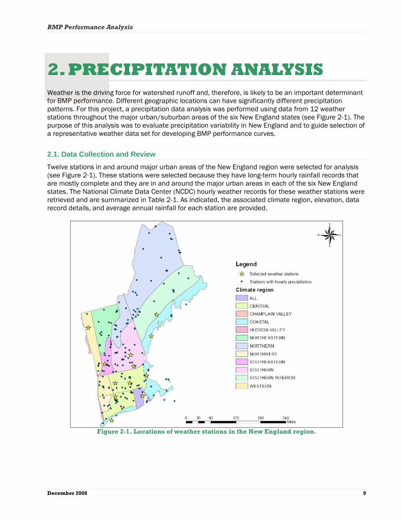
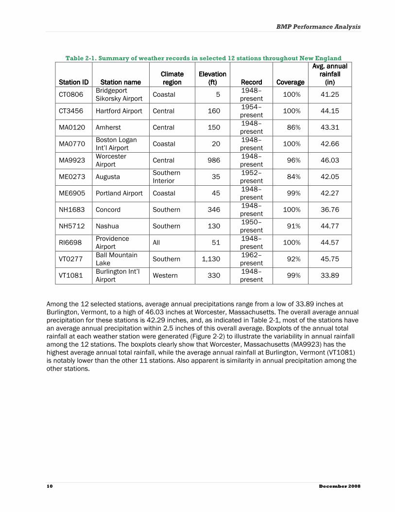
2. PRECIPITATION ANALYSIS Weather is the driving force for watershed runoff and, therefore, is likely to be an important determinant for BMP performance. Different geographic locations can have significantly different precipitation patterns. For this project, a precipitation data analysis was performed using data from 12 weather stations throughout the major urban/suburban areas of the six New England states (see Figure 2-1). The purpose of this analysis was to evaluate precipitation variability in New England and to guide selection of a representative weather data set for developing BMP performance curves.
2.1. Data Collection and Review
Twelve stations in and around major urban areas of the New England region were selected for analysis (see Figure 2-1). These stations were selected because they have long-term hourly rainfall records that are mostly complete and they are in and around the major urban areas in each of the six New England states. The National Climate Data Center (NCDC) hourly weather records for these weather stations were retrieved and are summarized in Table 2-1. As indicated, the associated climate region, elevation, data record details, and average annual rainfall for each station are provided.
Figure 2-1. Locations of weather stations in the New England region.
BMP Performance Analysis
10 December 2008
Table 2-1. Summary of weather records in selected 12 stations throughout New England
Station IDStation IDStation IDStation ID Station nameStation nameStation nameStation name Climate Climate Climate Climate regionregionregionregion
Elevation Elevation Elevation Elevation (ft)(ft)(ft)(ft) RecorRecorRecorRecordddd CoverageCoverageCoverageCoverage
AvAvAvAvgggg. annual . annual . annual . annual rainfallrainfallrainfallrainfall (in)(in)(in)(in)
CT0806 Bridgeport Sikorsky Airport
Coastal 5 1948–present
100% 41.25
CT3456 Hartford Airport Central 160 1954–present
100% 44.15
MA0120 Amherst Central 150 1948–present
86% 43.31
MA0770 Boston Logan Int’l Airport
Coastal 20 1948–present
100% 42.66
MA9923 Worcester Airport
Central 986 1948–present
96% 46.03
ME0273 Augusta Southern Interior
35 1952–present
84% 42.05
ME6905 Portland Airport Coastal 45 1948–present
99% 42.27
NH1683 Concord Southern 346 1948–present
100% 36.76
NH5712 Nashua Southern 130 1950–present
91% 44.77
RI6698 Providence Airport
All 51 1948–present
100% 44.57
VT0277 Ball Mountain Lake
Southern 1,130 1962–present
92% 45.75
VT1081 Burlington Int’l Airport
Western 330 1948–present
99% 33.89
Among the 12 selected stations, average annual precipitations range from a low of 33.89 inches at Burlington, Vermont, to a high of 46.03 inches at Worcester, Massachusetts. The overall average annual precipitation for these stations is 42.29 inches, and, as indicated in Table 2-1, most of the stations have an average annual precipitation within 2.5 inches of this overall average. Boxplots of the annual total rainfall at each weather station were generated (Figure 2-2) to illustrate the variability in annual rainfall among the 12 stations. The boxplots clearly show that Worcester, Massachusetts (MA9923) has the highest average annual total rainfall, while the average annual rainfall at Burlington, Vermont (VT1081) is notably lower than the other 11 stations. Also apparent is similarity in annual precipitation among the other stations.

BMP Performance Analysis
December 2008 11
0
10
20
30
40
50
60
70
80
CT
0808
Brid
geP
ort
CT
3456
Har
tford
MA
0120
Am
hers
t
MA
0770
Bos
ton
MA
9923
Wor
cest
er
ME
0273
Aug
usta
ME
6905
Por
tland
NH
1683
Con
cord
NH
5712
Nas
hua
RI6
698P
rovi
denc
e
VT
0277
Bal
lMou
ntai
nLak
e
VT
1081
Bur
lingt
on
Weather stations in the New England region
An
nu
al to
tal r
ain
fall
(in)
Figure 2-2. Boxplots of annual total rainfall for selected weather stations in New England.
2.2. Event Frequency Analysis
While annual average precipitation is an important factor to distinguish differences among stations, the distribution of precipitation events by size or depth is important too. Long-term BMP performance will be influenced by the number of small, medium, and large precipitation events (i.e., distribution) that the BMP treats. From a water quality perspective, BMPs will typically perform more effectively for smaller storms primarily because the BMPs operate below their designed hydraulic capacity. Therefore, a BMP placed in a location with mostly small events will likely have a different long-term cumulative performance than if it were placed in a location with mostly large events, even if both locations have similar annual average precipitations. A frequency analysis of the precipitation events by depth was performed for each of the 12 stations to further understand the variability of precipitation patterns in the New England region. The goal of the precipitation event frequency analysis is to identify how the precipitation events are distributed across different categories of total depth. Three rainfall depth categories were used in the frequency analysis: (1) lower than 0.1 inch, (2) 0.1 inch to 1 inch, and (3) higher than 1 inch. The total number of events and the corresponding percentage of the total number of events were determined for each size category for each of the 12 stations. The resulting precipitation event distributions are summarized in Table 2-2.

BMP Performance Analysis
12 December 2008
Table 2-2. Summary of precipitation event frequency distribution sorted by precipitation depth
Precipitation amount
(inches)
StaStaStaStation IDtion IDtion IDtion ID Station nameStation nameStation nameStation name <<<< 0.10.10.10.1 0.10.10.10.1––––1.01.01.01.0 >>>> 1111
CT0806 Bridgeport Sikorsky Airport 46% 46% 8%
CT3456 Hartford Airport 48% 44% 8%
MA0120 Amherst 45% 47% 8%
MA0770 Boston Logan Int’l Airport 49% 44% 7%
MA9923 Worcester Airport 48% 44% 8%
ME0273 Augusta 45% 47% 8%
ME6905 Portland Airport 49% 47% 8%
NH1683 Concord 49% 47% 5%
NH5712 Nashua 47% 45% 8%
RI6698 Providence Airport 48% 44% 8%
VT0277 Ball Mountain Lake 43% 49% 8%
VT1081 Burlington Int’l Airport 56% 41% 3%
Average of all stations 48% 45% 7% As indicated, there is similarity in the distributions of rainfall events among the twelve stations barring the Burlington, Vermont station. On average, 48 percent of the events are < 0.1 inch, 45 percent of the events are 0.1 to 1.0 inches, and only 7 percent are > 1.0 inch. The rainfall events with depths between 0.1 and 1.0 inch are the most significant in terms of pollutant loading from urban areas because of the high frequency of these sized events and because they generate enough runoff to wash off most of the pollutants that have accumulated on impervious surfaces. Rainfall events of 0.1 or less are frequent but are not significant in terms of pollutant loading because they generate very little, if any, runoff volume, even from impervious areas. Precipitation events greater than 1 inch are relatively infrequent, and although they generate large runoff volumes, most of the pollutant washoff occurs during the early portion of the storms so that water quality BMPs sized for smaller storms (< 1 inch) can still be highly effective at capturing the pollutant load. Weather data from the Boston, Massachusetts, station was selected to generate BMP performance estimates for this project. The Boston station (MA0770), in the Costal climate region and in a highly urbanized portion of eastern Massachusetts, has an average annual precipitation of 42.66 inches, which closely matches the overall average annual precipitation of 42.29 inches, as well as the annual precipitation of most of the other stations. The precipitation frequency distribution of the Boston station closely matches the distribution of the other stations except for the Burlington, Vermont, station. The Boston station is appropriate for assessing runoff conditions in the Boston metropolitan area of Massachusetts, which is one of the most urbanized areas in New England. Also, the NPDES permitting program for discharges in Massachusetts needs BMP performance estimates for designated urban areas to assess stormwater management plans developed under the NPDES stormwater permitting program.

BMP Performance Analysis
December 2008 13
While the Boston data set appears to be similar (in terms of annual precipitation and event distributions) to most of the data sets from the other stations, it would be useful for a future effort to test the sensitivity of predicted BMP performances to rainfall variability in New England by using data from a weather station that is the most different from the Boston data. On the basis of the analysis conducted for this project, the Burlington, Vermont (VT1081) data set would be a good candidate for evaluating how sensitive BMP performance is to different weather conditions in New England. The boxplots (Figure 2-3) of annual total rainfall from these weather stations (VT1081 and MA0770) illustrate the differences in annual precipitation between them. Also, the frequency distribution analysis reveals that the event distribution for Burlington, Vermont, is the most different from the event distribution of Boston, Massachusetts.
20
25
30
35
40
45
50
55
60
65
MA0770-Boston VT1081-Burlington
An
nu
al to
tal r
ain
fall
(in)
Figure 2-3. Recommended weather stations based on annual precipitation for evaluating BMP
performances.

BMP Performance Analysis
14 December 2008
3. LAND ANALYSIS
The goal of the land analysis was to generate the flow and pollutant time series (hydrographs and pollutographs) for each land use type. These time series were later used in the BMP modeling to estimate BMP performances. The land analysis involved selecting representative pollutant loading targets as well as selecting an appropriate the model to use for generating flows and pollutant time series.
3.1. Land Representation for Pollutant Loading
The ultimate goal for this project is to predict BMP performances on the basis of the capacity of BMPs to treat runoff depths (and corresponding volumes) generated by specified amounts of rainfall. Thus, the inflow and pollutant time series play an important role in determining the shape of final BMP performance curves. The approach used in this project to generate the pollutant loadings is similar to the approaches incorporated into widely used urban stormwater models such as the Storm Water Management Model (SWMM) (Huber and Dickinson 1988) and the P8-UCM (Walker 1990) and involves simulating the buildup and washoff of pollutants from impervious surfaces only. Using the impervious surfaces to generate pollutant loading greatly simplifies estimating loadings because it avoids having to represent a high number of combinations of pervious soil and land cover conditions. Also, impervious areas generate most of the runoff in urban/suburban catchments and pollutant load because accumulated pollutants are readily washed off of impervious surfaces. In contrast, runoff volumes and pollutant loads from pervious surfaces tends to be much lower and are highly variable because of attenuation by soils and vegetation. Moreover, the performance curves generated by this project are intended to apply to urban settings, which typically consist of highly impervious surfaces. The curves are expected to be most frequently used at a site-scale level where BMPs will be designed to treat runoff from developed impervious portions of sites (e.g., commercial center, streets, and parking lots). A further evaluation of the precipitation characteristics for Boston, Massachusetts, also supports the use of only impervious surfaces for generating pollutant time series. A detailed breakdown of rainfall depth frequency analysis for Boston is shown in Figure 3-1, which illustrates that most of the rain events that have occurred in Boston have been relatively small events (e.g., 84 percent of the events < 0.6 inches). To better appreciate the significance of the precipitation characteristics as it relates to impervious and pervious surfaces, a table of initial abstraction (Ia) for various pervious surfaces and hydrologic soils groups (HSG) is provided (see Table 3-1). Soils are assigned to an HSG on the basis of their permeability. HSG A is the most permeable, and HSG D is the least permeable. Ia values indicate the depth of rainfall that will not generate runoff. As indicated, pervious areas are not expected to generate runoff for most rainfall events in the Boston metropolitan region. For example, an open space area with fair condition and HSG C soils has an Ia of 0.53 inch. Therefore, such an area is not expected to generate runoff for rain events equal or less than 0.53 inches, which corresponds to 81 percent of all the rainfall events represented by the 56-year record. Also, rain events with 0.53 inch and less account for approximately 68 percent of the total rainfall volume for the same record. Figure 3-2 illustrates a cumulative frequency distribution for total precipitation volume based on precipitation depth. For stabilized urban and suburban areas, much of the annual pollutant load is believed to be generated from impervious areas because most of the runoff volume is generated by rainfall falling on impervious

BMP Performance Analysis
December 2008 15
areas and because pollutants that have been accumulated on impervious surfaces are readily washed off during even small rain events.
0.0 - 0.2 inches
0.2 - 0.6 inches
0.6 - 1.0 inches
1.0 - 1.5 inches
1.5 - 2.0 inches
2.0 inches and above
0.0 - 0.2 inches61%
1.0 - 1.5 inches4%
1.5 - 2.0 inches2%
0.6 - 1.0 inches9%
0.2 - 0.6 inches23%
2.0 inches and above 1%
Figure 3-1. Percentage of total number of precipitation events by size of precipitation events for
Boston, Massachusetts (1948–2004).

BMP Performance Analysis
16 December 2008
Figure 3-2. Cumulative distribution of total precipitation volume by rainfall depth for Boston,
Massachusetts (1948–2004).
Table 3-1. Ia values for various land use and HSGs
Initial abstractionInitial abstractionInitial abstractionInitial abstraction (inch)(inch)(inch)(inch)
Land use/cover conditionsLand use/cover conditionsLand use/cover conditionsLand use/cover conditions HSG AHSG AHSG AHSG A HSG BHSG BHSG BHSG B HSG CHSG CHSG CHSG C HSG DHSG DHSG DHSG D Poor (grass < 50%) 0.94 0.53 0.33 0.25 Fair (grass 50–75%) 2.08 0.90 0.53 0.38 Open space Good (grass > 75%) 3.13 1.28 0.70 0.50 1/8 acre or less 0.60 0.35 0.22 0.17
1/4 acre 1.28 0.67 0.41 0.30 1/3 acre 1.51 0.78 0.47 0.33 1/2 acre 1.70 0.86 0.50 0.35 1 acre 1.92 0.94 0.53 0.38
Residential
2 acres 2.35 1.08 0.60 0.44 Source: USDA-NRCS 1986
3.2. Selection of Water Quality Model
EPA’s Stormwater Management Model (SWMM) was selected for generating runoff volume and pollutant time series. The SWMM is a dynamic rainfall-runoff simulation model developed primarily for urban areas and can be used for both single-event and long-term (continuous) simulations using various time steps (Huber and Dickinson 1988). SWMM has the ability to analyze the buildup, washoff, and transport of a number of pollutants within a watershed for a long-term precipitation record (Rossman 2007). Four pollutants, total suspended solids (TSS), total phosphorus (TP), total nitrogen (TN), and zinc (Zn) were selected for this analysis because they are commonly associated with urban runoff and are responsible for numerous water quality problems in New England.
BMP Performance Analysis
December 2008 17
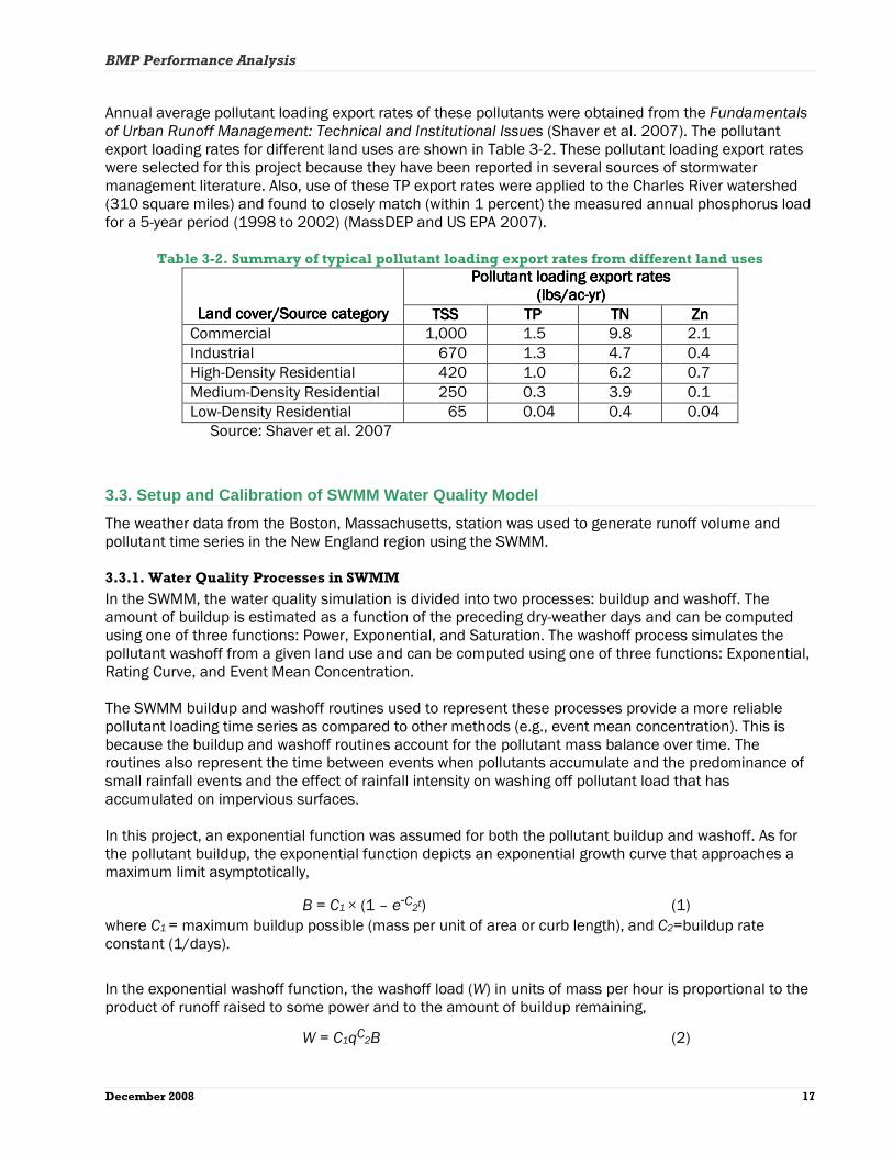
Annual average pollutant loading export rates of these pollutants were obtained from the Fundamentals of Urban Runoff Management: Technical and Institutional Issues (Shaver et al. 2007). The pollutant export loading rates for different land uses are shown in Table 3-2. These pollutant loading export rates were selected for this project because they have been reported in several sources of stormwater management literature. Also, use of these TP export rates were applied to the Charles River watershed (310 square miles) and found to closely match (within 1 percent) the measured annual phosphorus load for a 5-year period (1998 to 2002) (MassDEP and US EPA 2007).
Table 3-2. Summary of typical pollutant loading export rates from different land uses
Pollutant loadingPollutant loadingPollutant loadingPollutant loading export export export export raterateraterates s s s (lbs/ac(lbs/ac(lbs/ac(lbs/ac----yr)yr)yr)yr)
Land cover/SourceLand cover/SourceLand cover/SourceLand cover/Source category category category category TSSTSSTSSTSS TPTPTPTP TNTNTNTN ZnZnZnZn Commercial 1,000 1.5 9.8 2.1 Industrial 670 1.3 4.7 0.4 High-Density Residential 420 1.0 6.2 0.7 Medium-Density Residential 250 0.3 3.9 0.1 Low-Density Residential 65 0.04 0.4 0.04
Source: Shaver et al. 2007
3.3. Setup and Calibration of SWMM Water Quality Model
The weather data from the Boston, Massachusetts, station was used to generate runoff volume and pollutant time series in the New England region using the SWMM.
3.3.1. Water Quality Processes in SWMM
In the SWMM, the water quality simulation is divided into two processes: buildup and washoff. The amount of buildup is estimated as a function of the preceding dry-weather days and can be computed using one of three functions: Power, Exponential, and Saturation. The washoff process simulates the pollutant washoff from a given land use and can be computed using one of three functions: Exponential, Rating Curve, and Event Mean Concentration. The SWMM buildup and washoff routines used to represent these processes provide a more reliable pollutant loading time series as compared to other methods (e.g., event mean concentration). This is because the buildup and washoff routines account for the pollutant mass balance over time. The routines also represent the time between events when pollutants accumulate and the predominance of small rainfall events and the effect of rainfall intensity on washing off pollutant load that has accumulated on impervious surfaces. In this project, an exponential function was assumed for both the pollutant buildup and washoff. As for the pollutant buildup, the exponential function depicts an exponential growth curve that approaches a maximum limit asymptotically,
B = C1 × (1 – e-C2t) (1) where C1 = maximum buildup possible (mass per unit of area or curb length), and C2=buildup rate constant (1/days).
In the exponential washoff function, the washoff load (W) in units of mass per hour is proportional to the product of runoff raised to some power and to the amount of buildup remaining,
W = C1qC2B (2)
BMP Performance Analysis
18 December 2008
where C1 = washoff coefficient, C2 = washoff exponent, q = runoff rate per unit area (inches/hour [in/hr]), and B = pollutant buildup in mass (lbs) per unit area or curb length.
3.3.2. Setup and Calibration of SWMM
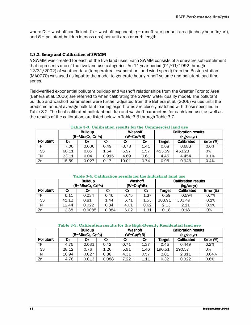
A SWMM was created for each of the five land uses. Each SWMM consists of a one-acre sub-catchment that represents one of the five land use categories. An 11-year period (01/01/1992 through 12/31/2002) of weather data (temperature, evaporation, and wind speed) from the Boston station (MA0770) was used as input to the model to generate hourly runoff volume and pollutant load time series. Field-verified exponential pollutant buildup and washoff relationships from the Greater Toronto Area (Behera et al. 2006) are referred to when calibrating the SWMM water quality model. The pollutant buildup and washoff parameters were further adjusted from the Behera et al. (2006) values until the predicted annual average pollutant loading export rates are closely matched with those specified in Table 3-2. The final calibrated pollutant buildup and washoff parameters for each land use, as well as the results of the calibration, are listed below in Table 3-3 through Table 3-7.
Table 3-3. Calibration results for the Commercial land use
BuildupBuildupBuildupBuildup (B=(B=(B=(B=MinMinMinMin(C(C(C(C1111, C, C, C, C2222ttttCCCC3333))))
Washoff Washoff Washoff Washoff (W=C(W=C(W=C(W=C1111qqqqCCCC2222B)B)B)B)
Calibration results Calibration results Calibration results Calibration results (kg/ac(kg/ac(kg/ac(kg/ac----yr)yr)yr)yr)
PollutantPollutantPollutantPollutant CCCC1111 CCCC2222 CCCC3333 CCCC1111 CCCC2222 TargetTargetTargetTarget CalibratedCalibratedCalibratedCalibrated Error (%)Error (%)Error (%)Error (%) TP 7.00 0.036 0.49 0.78 1.41 0.68 0.683 0.6% TSS 68.11 0.85 1.54 6.97 1.57 453.59 453.23 0% TN 23.11 0.04 0.915 4.69 0.61 4.45 4.454 0.1% Zn 15.59 0.027 0.17 10.01 0.74 0.95 0.946 0.4%
Table 3-4. Calibration results for the Industrial land use
BuildupBuildupBuildupBuildup (B=(B=(B=(B=MinMinMinMin(C(C(C(C1111, C, C, C, C2222ttttCCCC3333))))
Washoff Washoff Washoff Washoff (W=C(W=C(W=C(W=C1111qqqqCCCC2222B)B)B)B)
Calibration results Calibration results Calibration results Calibration results (kg/ac(kg/ac(kg/ac(kg/ac----yr)yr)yr)yr)
PollutantPollutantPollutantPollutant CCCC1111 CCCC2222 CCCC3333 CCCC1111 CCCC2222 TargetTargetTargetTarget CalibrCalibrCalibrCalibratedatedatedated Error (%)Error (%)Error (%)Error (%) TP 6.11 0.034 0.46 0.75 1.37 0.59 0.594 0.7% TSS 41.12 0.81 1.44 6.71 1.53 303.91 303.49 0.1% TN 12.44 0.022 0.84 4.01 0.62 2.13 2.11 0.9% Zn 2.38 0.0085 0.084 6.02 1.31 0.18 0.18 0%
Table 3-5. Calibration results for the High-Density Residential land use
BuildupBuildupBuildupBuildup (B=(B=(B=(B=MinMinMinMin(C(C(C(C1111, C, C, C, C2222ttttCCCC3333))))
Washoff Washoff Washoff Washoff (W=C(W=C(W=C(W=C1111qqqqCCCC2222B)B)B)B)
Calibration results Calibration results Calibration results Calibration results (kg/ac(kg/ac(kg/ac(kg/ac----yr)yr)yr)yr)
PollutantPollutantPollutantPollutant CCCC1111 CCCC2222 CCCC3333 CCCC1111 CCCC2222 TargetTargetTargetTarget CalibratedCalibratedCalibratedCalibrated Error (%)Error (%)Error (%)Error (%) TP 4.75 0.031 0.42 0.71 1.37 0.45 0.449 0.2% TSS 28.12 0.76 1.26 5.91 1.46 190.51 190.57 0% TN 18.94 0.027 0.88 4.31 0.57 2.81 2.811 0.04% Zn 4.78 0.013 0.088 7.22 1.11 0.32 0.322 0.6%

BMP Performance Analysis
December 2008 19
Table 3-6. Calibration results for the Medium-Density Residential land use
BuildupBuildupBuildupBuildup (B=(B=(B=(B=MinMinMinMin(C(C(C(C1111, C, C, C, C2222ttttCCCC3333))))
Washoff Washoff Washoff Washoff (W=C(W=C(W=C(W=C1111qqqqCCCC2222B)B)B)B)
Calibration results Calibration results Calibration results Calibration results (kg/ac(kg/ac(kg/ac(kg/ac----yr)yr)yr)yr)
PollutantPollutantPollutantPollutant CCCC1111 CCCC2222 CCCC3333 CCCC1111 CCCC2222 TargetTargetTargetTarget CalibratedCalibratedCalibratedCalibrated Error (%)Error (%)Error (%)Error (%) TP 1.77 0.027 0.31 0.43 1.27 0.229 0.225 1.7% TSS 19.48 0.62 1.12 5.11 1.21 113.40 113.50 0.1% TN 10.94 0.019 0.82 4.01 0.52 1.77 1.768 0.1% Zn 1.24 0.006 0.051 2.11 1.89 0.045 0.045 0%
Table 3-7. Calibration results for the Low-Density Residential land use
BuildupBuildupBuildupBuildup (B=(B=(B=(B=MinMinMinMin(C(C(C(C1111, C, C, C, C2222ttttCCCC3333))))
Washoff Washoff Washoff Washoff (W=C(W=C(W=C(W=C1111qqqqCCCC2222B)B)B)B)
Calibration results Calibration results Calibration results Calibration results (kg/ac(kg/ac(kg/ac(kg/ac----yr)yr)yr)yr)
PollutantPollutantPollutantPollutant CCCC1111 CCCC2222 CCCC3333 CCCC1111 CCCC2222 TargetTargetTargetTarget CalibratedCalibratedCalibratedCalibrated Error (%)Error (%)Error (%)Error (%) TP 0.27 0.0064 0.09 0.19 1.14 0.018 0.019 5.5% TSS 4.18 0.31 0.87 2.11 1.02 29.48 29.48 0% TN 8.44 0.0035 0.44 3.01 0.21 0.18 0.181 0.6% Zn 0.98 0.0039 0.021 1.47 2.35 0.018 0.019 5.5%
Following calibration of the SWMM for the land uses, model simulations were performed to generate runoff volume and pollutant time series for each land use. These time series were used as input to the BMP modeling system to predict long-term BMP performance (see Sections 4 and 5).

BMP Performance Analysis
20 December 2008
4. BMP ANALYSIS
The BMP analysis involves two major tasks designed to support the development of long-term performance curves for the following BMPs:
• Subsurface infiltration systems (infiltration trench)
• Surface infiltration systems (infiltration basin)
• Gravel wetland
• Bioretention systems
• Porous pavement
• Swales
• Dry detention ponds
• Wet ponds
The first task was to recalibrate and test BMPDSS for New England conditions using BMP performance data collected at the University of New Hampshire Stormwater Center (UNHSC). The second task evaluated BMP design criteria from the New England states and selected the design criteria for each BMP for use in the BMPDSS to develop long-term performance curves.
4.1. BMPDSS Calibration and Testing
Prince George’s County BMPDSS, was selected as the BMP model to simulate long-term pollutant removal performance of the selected BMPs. Performance curves were generated by varying the capacity or size (amount of runoff captured) of the BMPs. The BMPDSS model was recalibrated (BMPDSS was previously calibrated for Prince George’s County, Maryland) using BMP performance data collected by UNHSC to represent current data and New England conditions. Recalibration was performed for all the BMPs except for the dry detention pond because performance data for dry detention ponds were not available from UNHSC. This section details the BMPDSS calibration and testing task.
4.1.1. Overview of the Calibration Process
The calibration process involved adjusting BMP design parameters (porosity, infiltration rate, vegetation cover percentage, and so on) to best simulate the BMP’s hydraulic and pollutant removal performance. The goal of the calibration process was to match model hydrologic and water quality predictions with observed data for the calibration events. BMPDSS was calibrated for the following BMPs: (1) infiltration system, (2) gravel wetland, (3) bioretention system, (4) porous pavement, (5) grass swale, and (6) wet pond.
Calibrating a BMP using the BMPDSS model was a three-step process. First, the hydrologic and water quality time series were generated using SWMM. This involved calibrating SWMM to match the observed discrete inflow volume and water quality data. The calibrated SWMM was used to generate continuous hourly time series, which BMPDSS requires as input. Second, a hydraulic calibration of BMPDSS for each BMP was performed using the SWMM-generated inflow time series. During this process, the BMP’s hydrologic parameters (porosity, infiltration rate, vegetation cover percentage, and such) were adjusted as needed to achieve acceptable agreement between model predications and measured flow data. Finally, the water quality calibration of each BMP was completed by adjusting the water quality-related parameters (e.g., first order decay coefficients and filtering efficiencies). As with the hydraulic calibration,

BMP Performance Analysis
December 2008 21
the objective of the water quality calibration was to achieve acceptable agreement between BMPDSS predictions and measured BMP outflow pollutant concentrations.
Depending on the BMP, the water quality simulation can consider two mechanisms: general loss or decay of pollutant (by settling, plant uptake, volatilization, and such) and pollutant filtration through a substrate. For each type of BMP, the appropriate pollutant removal mechanisms were selected. For example, wet detention pond and swale BMPs include only the general loss component because the filtration mechanism is not applicable, whereas, bioretention, gravel wetland, infiltration system, and porous pavement BMPs include both general loss and filtration mechanisms.
The general loss or decay is represented using a first order decay model:
Ct = C0 e (-kt) (3)
where Ct is the pollutant concentration at time t, C0 is the initial pollutant concentration, and k is the first order decay rate (T-1).
Pollutant filtration through substrate is simulated using percent removal:
Cud_out = Prem Cin e (-kt) (4)
where Cud_out is the underdrain outflow pollutant concentration, Cin is pollutant concentration in inflow to the substrate, and Prem is media filtration percent removal rate (0–1). Figure 4-1 illustrates the water quality simulation processes that occur in a BMP unit in BMPDSS. Parameters k and Prem were adjusted during the water quality calibration process.
Figure 4-1. Water quality simulation processes.
For calibration, hydraulic and water quality parameters were adjusted for each BMP using three rainfall events with the goal of achieving the best match between model predictions and measured data for each event. The average of the adjusted hydraulic and water quality parameters for three events became the calibrated parameters for each BMP. Final testing of the BMPDSS model performance for each calibrated BMP was conducted by performing continuous simulations of the BMPDSS for the period of 2004–2006 and comparing the model predicted 2004–2006 BMP pollutant load reductions to the long-term BMP performances reported by UNHSC in its 2007 Annual Report (UNHSC 2007). The UNHSC calculated the long-term performance

BMP Performance Analysis
22 December 2008
using many monitoring events conducted over this period. This approach for testing the model’s performance using long-term performance model results and data is particularly appropriate because the calibrated BMPDSS models were used for long-term simulations in the performance curve generations. During the testing process, the calibrated BMPDSS model was applied for each BMP for the period of 2004–2006 using hourly flow and quality results from SWMM as input. Then the model-predicted total inflow pollutant load and outflow load for the period were determined to calculate the pollutant reduction percentages (see section 4.1.4).
4.1.2. BMPDSS Calibration Events
The calibration events for BMPDSS are summarized in Table 4-1. As shown, six events were selected for use in the BMP calibration process ensuring that performance data are available for at least three events for each BMP. SWMM was calibrated with observed inflow and inflow pollutant concentrations for each selected storm. Calibrated time series of flow and pollutant concentrations were then used as input into BMPDSS for the BMP calibration.
Table 4-1. Selection of calibration events for BMPs
1111 2222 3333 4444 5555 6666 BMP listBMP listBMP listBMP list 10/30/2004 8/13/2005 11/30/2005 1/12/2006 5/9/2006 6/21/2006 Bioretention area √ √ √ Grass swale √ √ √ Gravel wetland √ √ √ Infiltration system √ √ √ Porous pavement √ √ √ Wet pond √ √ √

BMP Performance Analysis
December 2008 23
4.1.3. BMPDSS calibration results
Hydrologic calibrations of the BMP was first performed, followed by the water quality calibrations for the selected pollutants TSS, TP, TN, and Zn. However, it was determined during the calibration that there was insufficient TN data to complete the calibration of the BMP models for TN. Therefore, TN was dropped from the project, and the water quality calibrations focused on TSS, TP, and Zn.
1. Infiltration system
Calibration for event 08/13/2005 The hydrologic calibration of the infiltration system for event 08/13/2005 is illustrated in Figure 4-2. The water quality calibration results for TSS, TP, and Zn are summarized in Table 4-2.
0
50
100
150
200
250
300
350
400
16:0
016
:40
17:2
018
:00
18:4
019
:20
20:0
020
:40
21:2
022
:00
22:4
023
:20
0:00
0:40
1:20
2:00
2:40
3:20
4:00
4:40
5:20
6:00
6:40
7:20
8:00
8:40
9:20
10:0
010
:40
Time
Flo
w (g
pm
)
Observed inflowGenerated inflow to infiltration systemObserved outflowCalibrated BMPDSS outflow
Figure 4-2. The hydrologic calibration of BMPDSS for infiltration system for event 08/13/2005.
Calibration for event 01/12/2006 The hydrologic calibration of the infiltration system for event 01/12/2006 is illustrated in Figure 4-3. The water quality calibration results for TSS, TP, and Zn are summarized in Table 4-2.
BMP Performance Analysis
24 December 2008
0
50
100
150
200
250
19:0
0
19:4
0
20:2
0
21:0
0
21:4
0
22:2
0
23:0
0
23:4
0
0:20
1:00
1:40
2:20
3:00
3:40
4:20
5:00
5:40
6:20
7:00
7:40
8:20
9:00
9:40
10:2
0
11:0
0
Time
Flo
w (g
pm
)
Observed inflowGenerated inflow to infiltration systemObserved outflowCalibrated BMPDSS outflow
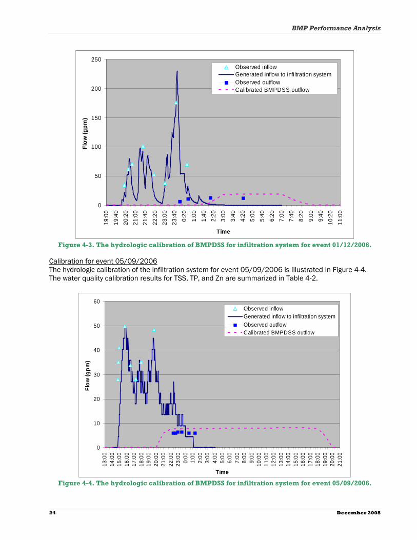
Figure 4-3. The hydrologic calibration of BMPDSS for infiltration system for event 01/12/2006.
Calibration for event 05/09/2006 The hydrologic calibration of the infiltration system for event 05/09/2006 is illustrated in Figure 4-4. The water quality calibration results for TSS, TP, and Zn are summarized in Table 4-2.
0
10
20
30
40
50
60
13:0
014
:00
15:0
016
:00
17:0
018
:00
19:0
020
:00
21:0
022
:00
23:0
00:
001:
002:
003:
004:
005:
006:
007:
008:
009:
0010
:00
11:0
012
:00
13:0
014
:00
15:0
016
:00
17:0
018
:00
19:0
020
:00
21:0
0
Time
Flo
w (g
pm
)
Observed inflowGenerated inflow to infiltration system
Observed outflowCalibrated BMPDSS outflow
Figure 4-4. The hydrologic calibration of BMPDSS for infiltration system for event 05/09/2006.

BMP Performance Analysis
December 2008 25
The individual calibrated pollutant decay rate and percent removal parameters for the three calibration events were averaged (Table 4-2) to determine the overall calibrated water quality parameters for the infiltration system.
Table 4-2. Summary of calibration results for infiltration system
PollutantsPollutantsPollutantsPollutants Calibration eventsCalibration eventsCalibration eventsCalibration events TSSTSSTSSTSS TPTPTPTP ZnZnZnZn
Inflow 72.13 0.16 0.11 Observed EMC (mg/L) Outflow 0.17 0.03 0
Calibrated outflow
0.17 0.03 0.006
Decay 0.76 0.31 0.47
08/13/2005 BMPDSS performance
Perct. removal 0.93 0.70 0.85 Inflow 52.06 0.10 0.03 Observed
EMC (mg/L) Outflow 0 0.01 0 Calibrated outflow
0.03 0.01 0.001
Decay 0.73 0.29 0.44
01/12/2006 BMPDSS performance
Perct. removal 0.90 0.65 0.81 Inflow 94.03 0.12 0.04 Observed
EMC (mg/L) Outflow 0 0.02 0 Calibrated outflow
0.01 0.02 0
Decay 0.73 0.21 0.44
05/09/2006 BMPDSS performance
Perct. removal 0.91 0.50 0.79 DecayDecayDecayDecay 0.740.740.740.74 0.270.270.270.27 0.450.450.450.45 Calibrated parametersCalibrated parametersCalibrated parametersCalibrated parameters Perct. removalPerct. removalPerct. removalPerct. removal 0.910.910.910.91 0.620.620.620.62 0.820.820.820.82

BMP Performance Analysis
26 December 2008
2. Gravel wetland
Calibration for event 08/13/2005 The hydrologic calibration of the gravel wetland for event 08/13/2005 is illustrated in Figure 4-5. The water quality calibration results for TSS, TP, and Zn are summarized in Table 4-3.
0
50
100
150
200
250
300
350
400
16:0
0
17:0
0
18:0
0
19:0
0
20:0
0
21:0
0
22:0
0
23:0
0
0:00
1:00
2:00
3:00
4:00
5:00
6:00
7:00
8:00
9:00
10:0
0
11:0
0
12:0
0
13:0
0
14:0
0
15:0
0
16:0
0
17:0
0
18:0
0
Time
Flo
w (g
pm
)
Observed inflowGenerated inflow to gravel wetlandObserved outflowCalibrated BMPDSS outflow
Figure 4-5. The hydrologic calibration of BMPDSS for gravel wetland for event 08/13/2005.
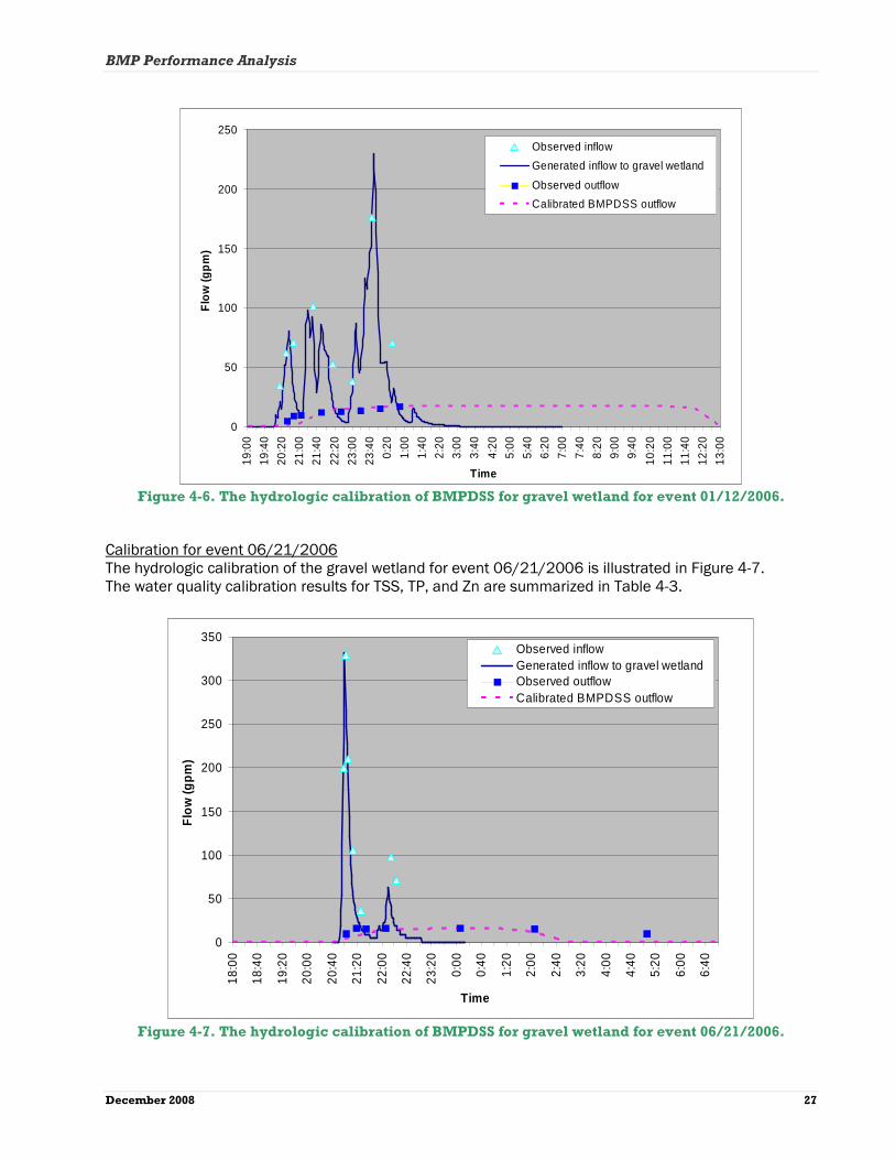
Calibration for event 01/12/2006 The hydrologic calibration of the gravel wetland for event 01/12/2006 is illustrated in Figure 4-6. The water quality calibration results for TSS, TP, and Zn are summarized in Table 4-3.
BMP Performance Analysis
December 2008 27
0
50
100
150
200
250
19:0
0
19:4
0
20:2
0
21:0
0
21:4
0
22:2
0
23:0
0
23:4
0
0:20
1:00
1:40
2:20
3:00
3:40
4:20
5:00
5:40
6:20
7:00
7:40
8:20
9:00
9:40
10:2
0
11:0
0
11:4
0
12:2
0
13:0
0
Time
Flo
w (g
pm
)
Observed inflow
Generated inflow to gravel wetland
Observed outflow
Calibrated BMPDSS outflow
Figure 4-6. The hydrologic calibration of BMPDSS for gravel wetland for event 01/12/2006.
Calibration for event 06/21/2006 The hydrologic calibration of the gravel wetland for event 06/21/2006 is illustrated in Figure 4-7. The water quality calibration results for TSS, TP, and Zn are summarized in Table 4-3.
0
50
100
150
200
250
300
350
18:0
0
18:4
0
19:2
0
20:0
0
20:4
0
21:2
0
22:0
0
22:4
0
23:2
0
0:00
0:40
1:20
2:00
2:40
3:20
4:00
4:40
5:20
6:00
6:40
Time
Flo
w (g
pm
)
Observed inflowGenerated inflow to gravel wetlandObserved outflowCalibrated BMPDSS outflow
Figure 4-7. The hydrologic calibration of BMPDSS for gravel wetland for event 06/21/2006.
BMP Performance Analysis
28 December 2008
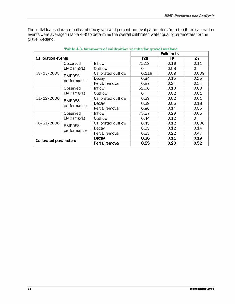
The individual calibrated pollutant decay rate and percent removal parameters from the three calibration events were averaged (Table 4-3) to determine the overall calibrated water quality parameters for the gravel wetland.
Table 4-3. Summary of calibration results for gravel wetland
PollutantsPollutantsPollutantsPollutants Calibration eventsCalibration eventsCalibration eventsCalibration events TSSTSSTSSTSS TPTPTPTP ZnZnZnZn
Inflow 72.13 0.16 0.11 Observed EMC (mg/L) Outflow 0 0.08 0
Calibrated outflow 0.116 0.08 0.008 Decay 0.34 0.15 0.25
08/13/2005 BMPDSS performance
Perct. removal 0.87 0.24 0.54 Inflow 52.06 0.10 0.03 Observed
EMC (mg/L) Outflow 0 0.02 0.01 Calibrated outflow 0.29 0.02 0.01 Decay 0.39 0.06 0.18
01/12/2006 BMPDSS performance
Perct. removal 0.86 0.14 0.55 Inflow 75.87 0.29 0.05 Observed
EMC (mg/L) Outflow 0.44 0.12 0 Calibrated outflow 0.45 0.12 0.006 Decay 0.35 0.12 0.14
06/21/2006 BMPDSS performance
Perct. removal 0.83 0.22 0.47 DecayDecayDecayDecay 0.360.360.360.36 0.110.110.110.11 0.190.190.190.19 Calibrated parametersCalibrated parametersCalibrated parametersCalibrated parameters Perct. removalPerct. removalPerct. removalPerct. removal 0.850.850.850.85 0.200.200.200.20 0.520.520.520.52

BMP Performance Analysis
December 2008 29
3. Bioretention area
Calibration for event 10/30/2004 The hydrologic calibration of the bioretention area for event 10/30/2004 is illustrated in Figure 4-8. The water quality calibration results for TSS, TP, and Zn are summarized in Table 4-4.
0
20
40
60
80
100
120
140
160
18015
:00
15:4
016
:20
17:0
017
:40
18:2
019
:00
19:4
020
:20
21:0
021
:40
22:2
023
:00
23:4
00:
201:
001:
402:
203:
003:
404:
205:
005:
406:
207:
007:
408:
209:
009:
4010
:20
11:0
011
:40
12:2
013
:00
13:4
0
Time
Flo
w (g
pm
)
Observed inflow
Generated inflow to bio-retention
Observed outflow
Calibrated BMPDSS outflow
Figure 4-8. The hydrologic calibration of BMPDSS for bioretention area for event 10/30/2004.
Calibration for event 05/09/2006 The hydrologic calibration of the bioretention area for event 05/09/2006 is illustrated in Figure 4-9. The water quality calibration results for TSS, TP, and Zn are summarized in Table 4-4.

BMP Performance Analysis
30 December 2008
0
10
20
30
40
50
60
13:0
0
13:4
0
14:2
0
15:0
0
15:4
0
16:2
0
17:0
0
17:4
0
18:2
0
19:0
0
19:4
0
20:2
0
21:0
0
21:4
0
22:2
0
23:0
0
23:4
0
0:20
1:00
1:40
2:20
3:00
3:40
4:20
5:00
5:40
6:20
7:00
7:40
Time
Flo
w (g
pm
)
Observed inflowGenerated inflow to bio-retention areaObserved outflowCalibrated BMPDSS outflow
Figure 4-9. The hydrologic calibration of BMPDSS for bioretention area for event 05/09/2006.
Calibration for event 06/21/2006 The hydrologic calibration of the bioretention area for event 06/21/2006 is illustrated in Figure 4-10. The water quality calibration results for TSS, TP, and Zn are summarized in Table 4-4.
0
50
100
150
200
250
300
350
20:0
0
20:2
0
20:4
0
21:0
0
21:2
0
21:4
0
22:0
0
22:2
0
22:4
0
23:0
0
23:2
0
23:4
0
0:00
0:20
0:40
1:00
1:20
1:40
2:00
2:20
2:40
3:00
Time
Flo
w (g
pm
)
Observed inflow
Generated inflow to bio-retention area
Observed outflow
Calibrated BMPDSS outflow
Figure 4-10. The hydrologic calibration of BMPDSS for bioretention area for event 06/21/2006.

BMP Performance Analysis
December 2008 31
The individual calibrated pollutant decay rate and percent removal parameters from the three events were averaged (Table 4-4) to determine the overall calibrated water quality parameters for the bioretention area.
Table 4-4. Summary of calibration results for bioretention area
PollutantsPollutantsPollutantsPollutants Calibration eventsCalibration eventsCalibration eventsCalibration events TSSTSSTSSTSS TPTPTPTP ZnZnZnZn
Inflow 32.56 0.02 0.08 Observed EMC (mg/L) Outflow 0.56 0 0
Calibrated outflow 0.56 0.02 0.002 Decay 0.62 0.13 0.49
10/30/2004 BMPDSS performance
Perct. removal 0.74 0.48 0.84 Inflow 94.03 0.12 0.04 Observed
EMC (mg/L) Outflow 0 0.12 0 Calibrated outflow 1.3 0.12 0.003 Decay 0.92 0.17 0.49
05/09/2006 BMPDSS performance
Perct. removal 0.98 0.50 0.84 Inflow 75.87 0.29 0.05 Observed
EMC (mg/L) Outflow 0 0.16 0 Calibrated outflow 0.20 0.16 0.001 Decay 0.82 0.10 0.49
06/21/2006 BMPDSS performance
Perct. removal 0.95 0.31 0.84 DecayDecayDecayDecay 0.790.790.790.79 0.130.130.130.13 0.490.490.490.49 Calibrated parametersCalibrated parametersCalibrated parametersCalibrated parameters Perct.Perct.Perct.Perct. removal removal removal removal 0.890.890.890.89 0.430.430.430.43 0.840.840.840.84

BMP Performance Analysis
32 December 2008
4. Porous pavement
Calibration for event 08/13/2005 The hydrologic calibration of the porous pavement for event 08/13/2005 is illustrated in Figure 4-11. The water quality calibration results for TSS, TP, and Zn are summarized in Table 4-5.
0
50
100
150
200
250
300
350
400
16:0
0
17:2
0
18:4
0
20:0
0
21:2
0
22:4
0
0:00
1:20
2:40
4:00
5:20
6:40
8:00
9:20
10:4
0
12:0
0
13:2
0
14:4
0
16:0
0
17:2
0
18:4
0
20:0
0
21:2
0
22:4
0
Time
Flo
w (g
pm
)
Observed inflowGenerated inflow to porous pavementObserved outflowCalibrated BMPDSS outflow
Figure 4-11. The hydrologic calibration of BMPDSS for porous pavement for event 08/13/2005.
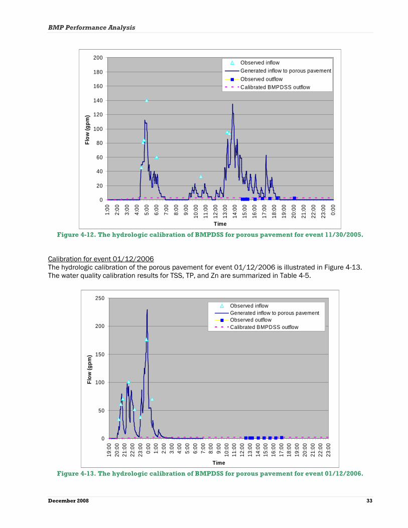
Calibration for event 11/30/2005 The hydrologic calibration of the porous pavement for event 11/30/2005 is illustrated in Figure 4-12. The water quality calibration results for TSS, TP, and Zn are summarized in Table 4-5.
BMP Performance Analysis
December 2008 33
0
20
40
60
80
100
120
140
160
180
200
1:00
2:00
3:00
4:00
5:00
6:00
7:00
8:00
9:00
10:0
0
11:0
0
12:0
0
13:0
0
14:0
0
15:0
0
16:0
0
17:0
0
18:0
0
19:0
0
20:0
0
21:0
0
22:0
0
23:0
0
0:00
Time
Flo
w (g
pm
)
Observed inflowGenerated inflow to porous pavement
Observed outflowCalibrated BMPDSS outflow
Figure 4-12. The hydrologic calibration of BMPDSS for porous pavement for event 11/30/2005.
Calibration for event 01/12/2006 The hydrologic calibration of the porous pavement for event 01/12/2006 is illustrated in Figure 4-13. The water quality calibration results for TSS, TP, and Zn are summarized in Table 4-5.
0
50
100
150
200
250
19:0
020
:00
21:0
022
:00
23:0
00:
001:
002:
003:
004:
005:
006:
007:
008:
009:
0010
:00
11:0
012
:00
13:0
014
:00
15:0
016
:00
17:0
018
:00
19:0
020
:00
21:0
022
:00
23:0
0
Time
Flo
w (g
pm
)
Observed inflowGenerated inflow to porous pavementObserved outflowCalibrated BMPDSS outflow
Figure 4-13. The hydrologic calibration of BMPDSS for porous pavement for event 01/12/2006.

BMP Performance Analysis
34 December 2008
The individual calibrated pollutant decay rate and percent removal parameters from the three calibration events were averaged (Table 4-5) to determine the overall calibrated water quality parameters for the porous pavement.
Table 4-5. Summary of calibration results for porous pavement
PollutantsPollutantsPollutantsPollutants Calibration eventsCalibration eventsCalibration eventsCalibration events TSSTSSTSSTSS TPTPTPTP ZnZnZnZn
Inflow 72.13 0.16 0.11 Observed EMC (mg/L) Outflow 0 0.04 0
Calibrated outflow 0.59 0.04 0.006 Decay 0.17 0.0053 0.11
08/13/2005 BMPDSS performance
Perct. removal 0.53 0.11 0.24 Inflow 17.31 0.09 0.03 Observed
EMC (mg/L) Outflow 0 0.06 0 Calibrated outflow 0.94 0.06 0.01 Decay 0.23 0.006 0.17
11/30/2005 BMPDSS performance
Perct. removal 0.84 0.11 0.31 Inflow 52.06 0.10 0.03 Observed
EMC (mg/L) Outflow 0 0.04 0.05 Calibrated outflow 0.92 0.04 0.05 Decay 0.27 0.004 0.14
01/12/2006 BMPDSS performance
Perct. removal 0.88 0.09 0.29 DecayDecayDecayDecay 0.220.220.220.22 0.00510.00510.00510.0051 0.140.140.140.14 Calibrated parametersCalibrated parametersCalibrated parametersCalibrated parameters Perct. removalPerct. removalPerct. removalPerct. removal 0.750.750.750.75 0.10.10.10.1 0.280.280.280.28
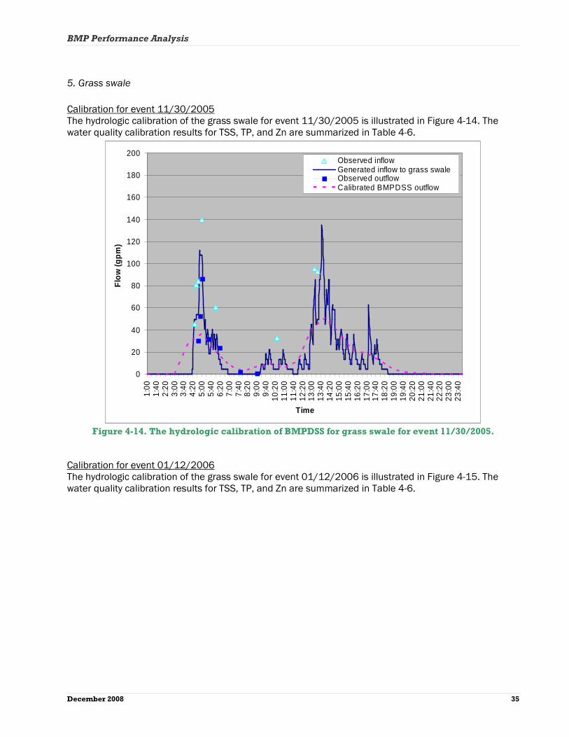
BMP Performance Analysis
December 2008 35
5. Grass swale
Calibration for event 11/30/2005 The hydrologic calibration of the grass swale for event 11/30/2005 is illustrated in Figure 4-14. The water quality calibration results for TSS, TP, and Zn are summarized in Table 4-6.
0
20
40
60
80
100
120
140
160
180
2001:
001:
402:
203:
003:
404:
205:
005:
406:
207:
007:
408:
209:
009:
4010
:20
11:0
011
:40
12:2
013
:00
13:4
014
:20
15:0
015
:40
16:2
017
:00
17:4
018
:20
19:0
019
:40
20:2
021
:00
21:4
022
:20
23:0
023
:40
Time
Flo
w (g
pm
)
Observed inflowGenerated inflow to grass swaleObserved outflowCalibrated BMPDSS outflow
Figure 4-14. The hydrologic calibration of BMPDSS for grass swale for event 11/30/2005.
Calibration for event 01/12/2006 The hydrologic calibration of the grass swale for event 01/12/2006 is illustrated in Figure 4-15. The water quality calibration results for TSS, TP, and Zn are summarized in Table 4-6.
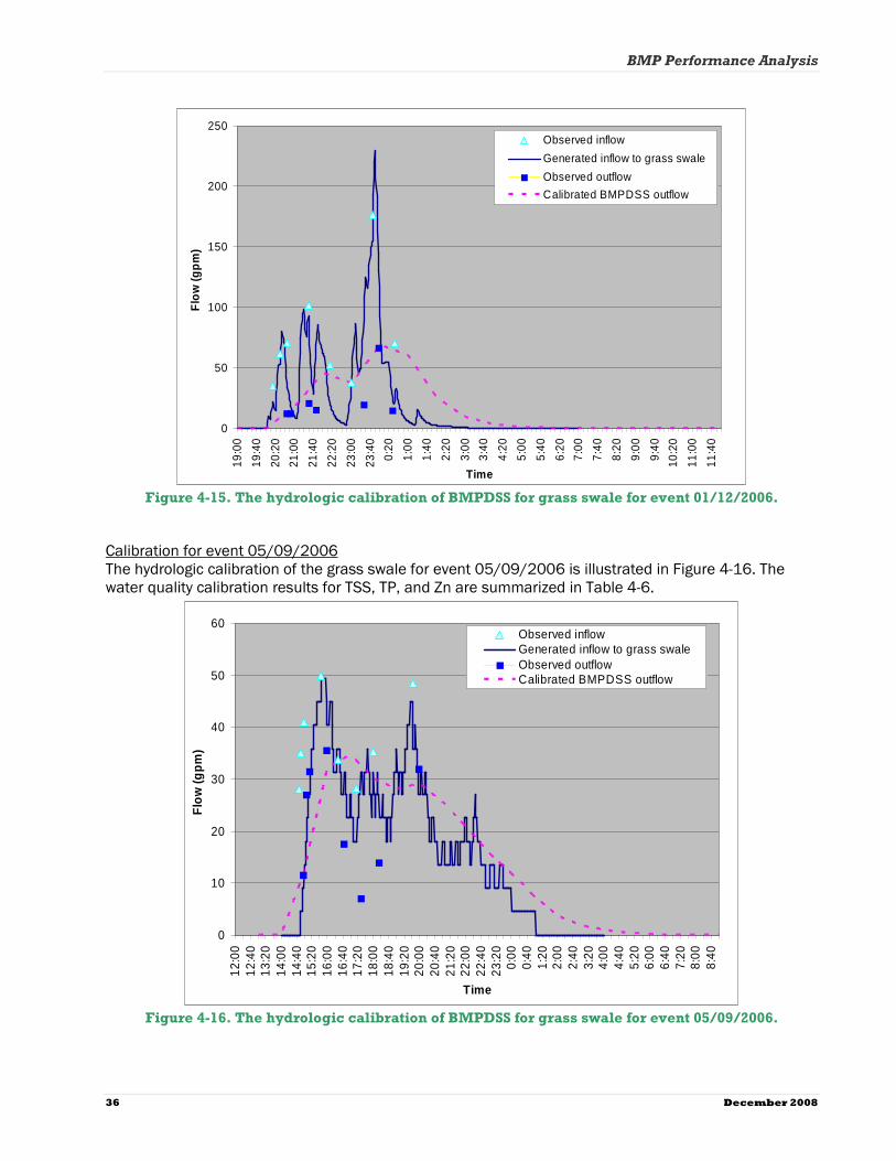
BMP Performance Analysis
36 December 2008
0
50
100
150
200
250
19:0
0
19:4
0
20:2
0
21:0
0
21:4
0
22:2
0
23:0
0
23:4
0
0:20
1:00
1:40
2:20
3:00
3:40
4:20
5:00
5:40
6:20
7:00
7:40
8:20
9:00
9:40
10:2
0
11:0
0
11:4
0
Time
Flo
w (g
pm
)
Observed inflow
Generated inflow to grass swale
Observed outflow
Calibrated BMPDSS outflow
Figure 4-15. The hydrologic calibration of BMPDSS for grass swale for event 01/12/2006.
Calibration for event 05/09/2006 The hydrologic calibration of the grass swale for event 05/09/2006 is illustrated in Figure 4-16. The water quality calibration results for TSS, TP, and Zn are summarized in Table 4-6.
0
10
20
30
40
50
60
12:0
012
:40
13:2
014
:00
14:4
015
:20
16:0
016
:40
17:2
018
:00
18:4
019
:20
20:0
020
:40
21:2
022
:00
22:4
023
:20
0:00
0:40
1:20
2:00
2:40
3:20
4:00
4:40
5:20
6:00
6:40
7:20
8:00
8:40
Time
Flo
w (g
pm
)
Observed inflowGenerated inflow to grass swaleObserved outflowCalibrated BMPDSS outflow
Figure 4-16. The hydrologic calibration of BMPDSS for grass swale for event 05/09/2006.

BMP Performance Analysis
December 2008 37
The individual calibrated pollutant decay rate and percent removal parameters from the three calibration events were averaged (Table 4-6) to determine the overall calibrated water quality parameters for the grass swale.
Table 4-6. Summary of calibration results for grass swale
PollutantsPollutantsPollutantsPollutants Calibration eventsCalibration eventsCalibration eventsCalibration events TSSTSSTSSTSS TPTPTPTP ZnZnZnZn
Inflow 17.31 0.09 0.03 Observed EMC (mg/L) Outflow 20.88 0.17 0.02
Calibrated outflow 20.71 0.16 0.02 Decay 0.93 0.04 2.15
11/30/2005 BMPDSS performance
Perct. removal N/A N/A N/A Inflow 52.06 0.10 0.03 Observed
EMC (mg/L) Outflow 45.05 0.10 0.03 Calibrated outflow 41.44 0.16 0.03 Decay 0.20 0.17 0.85
01/12/2006 BMPDSS performance
Perct. removal N/A N/A N/A Inflow 94.03 0.12 0.04 Observed
EMC (mg/L) Outflow 0.5 0.08 0 Calibrated outflow 0.5 0.07 0.008 Decay 0.85 0.10 2.35
05/09/2006 BMPDSS performance
Perct. removal N/A N/A N/A DecayDecayDecayDecay 0.660.660.660.66 0.100.100.100.10 1.781.781.781.78 Calibrated parametersCalibrated parametersCalibrated parametersCalibrated parameters Perct. removalPerct. removalPerct. removalPerct. removal N/AN/AN/AN/A N/AN/AN/AN/A N/AN/AN/AN/A

BMP Performance Analysis
38 December 2008
6. Wet pond
Calibration for event 08/13/2005 The hydrologic calibration of the wet pond for event 08/13/2005 is illustrated in Figure 4-17. The water quality calibration results for TSS, TP, and Zn are summarized in Table 4-7.
0
50
100
150
200
250
300
350
400
17:0
0
18:0
0
19:0
0
20:0
0
21:0
0
22:0
0
23:0
0
0:00
1:00
2:00
3:00
4:00
5:00
6:00
7:00
8:00
9:00
10:0
0
11:0
0
12:0
0
13:0
0
14:0
0
15:0
0
16:0
0
17:0
0
Time
Flo
w (g
pm
)
Observed inflowGenerated inflow to wet pondObserved outflowCalibrated BMPDSS outflow
Figure 4-17. The hydrologic calibration of BMPDSS for wet pond for event 08/13/2005.
Calibration for event 05/09/2006 The hydrologic calibration of the wet pond for event 05/09/2006 is illustrated in Figure 4-18. The water quality calibration results for TSS, TP, and Zn are summarized in Table 4-7.

BMP Performance Analysis
December 2008 39
0
10
20
30
40
50
60
13:0
014
:00
15:0
016
:00
17:0
018
:00
19:0
020
:00
21:0
022
:00
23:0
00:
001:
002:
003:
004:
005:
006:
007:
008:
009:
0010
:00
11:0
012
:00
13:0
014
:00
15:0
016
:00
17:0
018
:00
Time
Flo
w (g
pm
)
Observed inflowGenerated inflow to wet pondObserved outflowCalibrated BMPDSS outflow
Figure 4-18. The hydrologic calibration of BMPDSS for wet pond for event 05/09/2006.
Calibration for event 06/21/2006 The hydrologic calibration of the wet pond for event 06/21/2006 is illustrated in Figure 4-19. The water quality calibration results for TSS, TP, and Zn are summarized in Table 4-7.
0
50
100
150
200
250
300
350
20:0
0
21:0
0
22:0
0
23:0
0
0:00
1:00
2:00
3:00
4:00
5:00
6:00
7:00
8:00
9:00
10:0
0
11:0
0
12:0
0
13:0
0
14:0
0
15:0
0
16:0
0
Time
Flo
w (g
pm
)
Observed inflowGenerated inflow to wet pondObserved outflowCalibrated BMPDSS outflow
Figure 4-19. The hydrologic calibration of BMPDSS for wet pond for event 06/21/2006.

BMP Performance Analysis
40 December 2008
The individual calibrated pollutant decay rate and percent removal parameters from the three calibration events were averaged (Table 4-7) to determine the overall calibrated water quality parameters for the wet pond.
Table 4-7. Summary of calibration results for wet pond
PollutanPollutanPollutanPollutantstststs Calibration eventsCalibration eventsCalibration eventsCalibration events TSSTSSTSSTSS TPTPTPTP ZnZnZnZn
Inflow 72.13 0.16 0.11 Observed EMC (mg/L) Outflow 47.62 0.14 0.02
Calibrated outflow 47.36 0.14 0.02 Decay 0.20 0.01 1.40
08/13/2005 BMPDSS performance
Perct. removal N/A N/A N/A Inflow 94.03 0.12 0.04 Observed
EMC (mg/L) Outflow 0.8 0.04 0.005 Calibrated outflow 0.8 0.04 0.005 Decay 0.40 0.03 1.50
05/09/2006 BMPDSS performance
Perct. removal N/A N/A N/A Inflow 75.87 0.29 0.05 Observed
EMC (mg/L) Outflow 34.03 0.21 0 Calibrated outflow 34.23 0.21 0.003 Decay 0.18 0.05 1.69
06/21/2006 BMPDSS performance
Perct. removal N/A N/A N/A DecayDecayDecayDecay 0.260.260.260.26 0.030.030.030.03 1.531.531.531.53 Calibrated parametersCalibrated parametersCalibrated parametersCalibrated parameters Perct. removalPerct. removalPerct. removalPerct. removal N/AN/AN/AN/A N/AN/AN/AN/A N/AN/AN/AN/A

BMP Performance Analysis
December 2008 41
4.1.4. BMPDSS Test Results
The calibrated BMPDSS models performances were tested by comparing the model simulated long-term pollutant removal for the 2004–2006 period to the UNHSC reported long-term BMP performances reported for the same period. The calibrated BMPDSS models were run for the 2004–2006 period, and the pollutant removal rates of each BMP were calculated and compared to the UNHSC-reported values (UNHSC 2007). It is important to note that the UNHSC-reported values represent the median pollutant removal of selected storms (approximately 17–20 storms) for each BMP. BMPDSS-simulated pollutant removal reports the cumulative pollutant removal of all storms (34 storms) that occurred during the selected period including those analyzed by UNHSC.
1. Infiltration system
The test results of the infiltration system BMPDSS model are shown in Table 4-8. As shown, the BMPDSS model simulation results for TSS, TP, and Zn removal are similar to the UNHSC-reported values.
Table 4-8. Test results of infiltration system removal efficiencies for 2004–2006
Total pollutant loadTotal pollutant loadTotal pollutant loadTotal pollutant load TSSTSSTSSTSS (lbs)(lbs)(lbs)(lbs)
TPTPTPTP (lbs)(lbs)(lbs)(lbs)
ZnZnZnZn (lbs)(lbs)(lbs)(lbs)
Inflow 279.29 2.81 0.45 Outflow 4.21 0.48 0.01
Pollutant removal 98% 83% 98% UNHSC-report percentage 99% 81% 99%
2. Gravel wetland
The test results of the gravel wetland BMPDSS model are shown in Table 4-9. As shown, the BMPDSS model simulation results for TSS, TP, and Zn removal are similar to the UNHSC-reported values.
Table 4-9. Test results of gravel wetland removal efficiencies for 2004–2006
Total pollutant loadTotal pollutant loadTotal pollutant loadTotal pollutant load TSSTSSTSSTSS (lbs)(lbs)(lbs)(lbs)
TPTPTPTP (lbs)(lbs)(lbs)(lbs)
ZnZnZnZn (lbs)(lbs)(lbs)(lbs)
Inflow 279.29 2.81 0.45 Outflow 4.61 1.05 0.04
Pollutant removal 98% 63% 91% UNHSC-report percentage 99% 55% 99%
3. Bioretention area
The test results of the bioretention area BMPDSS model are shown in Table 4-10. As shown, the BMPDSS model simulation results for TSS and Zn are similar (< 5 percent difference) to the UNHSC-reported values. However, the BMPDSS model simulated a much higher long-term pollutant removal rate for TP than the UNHSC-reported value. The bioretention system at UNHSC has gone through several design and construction related issues during the selected period. The observed data could have been influenced by these uncertainties. A review of bioretention performance data reported by others indicates that the UNHSC-reported TP removal of 5 percent is relatively low for a well-functioning bioretention type of BMP. Consequently, the bioretention module in the existing BMPDSS, which was calibrated to bioretention performance data from the University of Maryland (Tetra Tech 2007) has resulted in a long-term TP

BMP Performance Analysis
42 December 2008
removal of 64 percent. The BMPDSS model prediction for TP removal appears to be reasonable when compared to the pollutant removal percentages reported by EPA for bioretention systems (USEPA 1999), which is 70–83 percent.
Table 4-10. Test results of bioretention area removal efficiencies for 2004–2006
TotTotTotTotal pollutant loadal pollutant loadal pollutant loadal pollutant load TSS TSS TSS TSS (lbs)(lbs)(lbs)(lbs)
TP TP TP TP (lbs)(lbs)(lbs)(lbs)
Zn Zn Zn Zn (lbs)(lbs)(lbs)(lbs)
Inflow 279.29 2.81 0.45 Outflow 15.82 1.13 0.02
Pollutant removal 94% 60% 96% UNHSC-reported percentage 99% 5% 99%
4. Porous pavement
The test results of the porous pavement BMPDSS model are shown in Table 4-11. As shown, the BMPDSS model simulation results for TSS, TP, and Zn removal are similar to the UNHSC-reported values.
Table 4-11. Test results of porous pavement removal efficiencies for 2004–2006
Total pollutant loadTotal pollutant loadTotal pollutant loadTotal pollutant load TSS TSS TSS TSS (lbs)(lbs)(lbs)(lbs)
TP TP TP TP (lbs)(lbs)(lbs)(lbs)
Zn Zn Zn Zn (lb(lb(lb(lbs)s)s)s)
Inflow 279.29 2.81 0.45 Outflow 5.46 1.58 0.04
Pollutant removal 98% 43% 92% UNHSC-reported percentage 99% 38% 96%
5. Grass swale
The test results of the grass swale BMPDSS model are shown in Table 4-12. As shown, the BMPDSS model simulation results for TSS, TP, and Zn removal are similar to the UNHSC-reported values.
Table 4-12. Test results of grass swale removal efficiencies for 2004–2006
Total pollutant loadTotal pollutant loadTotal pollutant loadTotal pollutant load TSS TSS TSS TSS (lbs)(lbs)(lbs)(lbs)
TP TP TP TP (lbs)(lbs)(lbs)(lbs)
Zn Zn Zn Zn (lbs)(lbs)(lbs)(lbs)
Inflow 279.29 2.81 0.45 Outflow 87.87 2.01 0.08
Pollutant removal 69% 29% 83% UNHSC-reported percentage 60% NT 88%
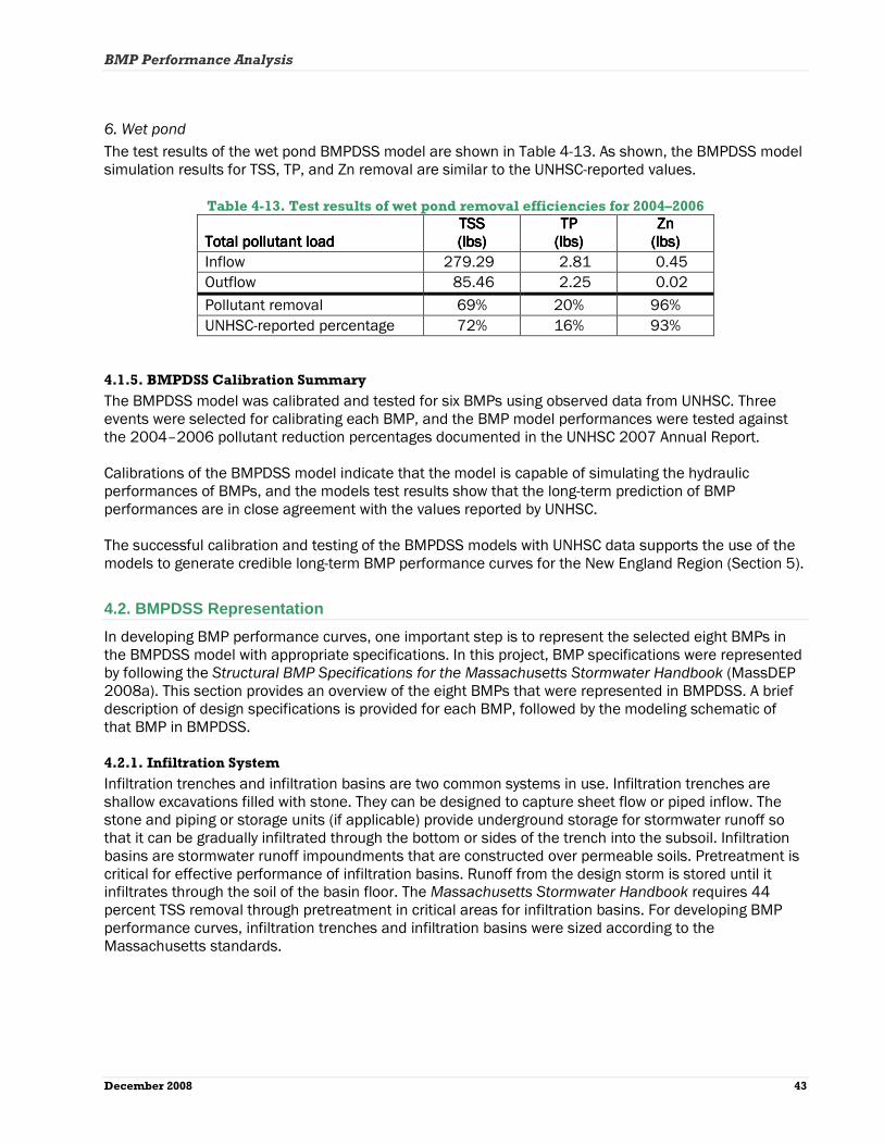
BMP Performance Analysis
December 2008 43
6. Wet pond
The test results of the wet pond BMPDSS model are shown in Table 4-13. As shown, the BMPDSS model simulation results for TSS, TP, and Zn removal are similar to the UNHSC-reported values.
Table 4-13. Test results of wet pond removal efficiencies for 2004–2006
Total pollutant loadTotal pollutant loadTotal pollutant loadTotal pollutant load TSS TSS TSS TSS (lbs)(lbs)(lbs)(lbs)
TP TP TP TP (lbs)(lbs)(lbs)(lbs)
Zn Zn Zn Zn (lbs)(lbs)(lbs)(lbs)
Inflow 279.29 2.81 0.45 Outflow 85.46 2.25 0.02
Pollutant removal 69% 20% 96% UNHSC-reported percentage 72% 16% 93%
4.1.5. BMPDSS Calibration Summary
The BMPDSS model was calibrated and tested for six BMPs using observed data from UNHSC. Three events were selected for calibrating each BMP, and the BMP model performances were tested against the 2004–2006 pollutant reduction percentages documented in the UNHSC 2007 Annual Report. Calibrations of the BMPDSS model indicate that the model is capable of simulating the hydraulic performances of BMPs, and the models test results show that the long-term prediction of BMP performances are in close agreement with the values reported by UNHSC. The successful calibration and testing of the BMPDSS models with UNHSC data supports the use of the models to generate credible long-term BMP performance curves for the New England Region (Section 5).
4.2. BMPDSS Representation
In developing BMP performance curves, one important step is to represent the selected eight BMPs in the BMPDSS model with appropriate specifications. In this project, BMP specifications were represented by following the Structural BMP Specifications for the Massachusetts Stormwater Handbook (MassDEP 2008a). This section provides an overview of the eight BMPs that were represented in BMPDSS. A brief description of design specifications is provided for each BMP, followed by the modeling schematic of that BMP in BMPDSS.
4.2.1. Infiltration System
Infiltration trenches and infiltration basins are two common systems in use. Infiltration trenches are shallow excavations filled with stone. They can be designed to capture sheet flow or piped inflow. The stone and piping or storage units (if applicable) provide underground storage for stormwater runoff so that it can be gradually infiltrated through the bottom or sides of the trench into the subsoil. Infiltration basins are stormwater runoff impoundments that are constructed over permeable soils. Pretreatment is critical for effective performance of infiltration basins. Runoff from the design storm is stored until it infiltrates through the soil of the basin floor. The Massachusetts Stormwater Handbook requires 44 percent TSS removal through pretreatment in critical areas for infiltration basins. For developing BMP performance curves, infiltration trenches and infiltration basins were sized according to the Massachusetts standards.
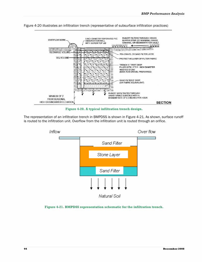
BMP Performance Analysis
44 December 2008
Figure 4-20 illustrates an infiltration trench (representative of subsurface infiltration practices)
Figure 4-20. A typical infiltration trench design.
The representation of an infiltration trench in BMPDSS is shown in Figure 4-21. As shown, surface runoff is routed to the infiltration unit. Overflow from the infiltration unit is routed through an orifice.
Figure 4-21. BMPDSS representation schematic for the infiltration trench.

BMP Performance Analysis
December 2008 45
A list of major parameters for the Figure 4-21 representation is summarized in Table 4-14.
Table 4-14. Design parameters for representing the infiltration trench in BMPDSS
Components of representationComponents of representationComponents of representationComponents of representation Design parametersDesign parametersDesign parametersDesign parameters ValueValueValueValue Porosity 0.40
Sand filter Depth 6 in Depth 6 feet
Infiltration Unit Stone layer
Porosity 0.45 The treatment capacity depends on the infiltration rate of soil at the bottom of the system. Therefore, BMP performance curves were developed for six different infiltration rates, 0.17, 0.27, 0.52, 1.02, 2.41, and 8.27 in/hr. Using the runoff volumes to be treated, the surface areas of the infiltration trench were estimated. To develop the curves, first the infiltration systems were sized with a physical storage capacity of 0.2, 0.4, 0.6, 0.8, 1.0, 1.5, and 2.0 inches of runoff volume from the contributing impervious surfaces. Next, long-term continuous simulations were performed using BMPDSS for a 10-year period to determine the cumulative pollutant load removed for TP, TSS, and Zn. Finally, for each of the BMP sizes simulated, the cumulative pollutant removal performance (expressed as % removed) was plotted against the corresponding BMP size. Figure 4-22 illustrates an infiltration basin (representative of a surface infiltration system).
Figure 4-22. Typical design of an infiltration basin.

BMP Performance Analysis
46 December 2008
A representation of the infiltration basin in BMPDSS is shown in Figure 4-23. As shown, surface runoff is routed to the infiltration unit. Overflow from the infiltration unit is routed through a weir.
Figure 4-23. BMPDSS representation of infiltration basin
When representing the infiltration basin in BMPDSS, the depth of the infiltration basin was set at 2 feet. The surface area of the infiltration basin was initially sized according to the Simple Dynamic method and using the equation on page 19, chapter 1, volume 3 of Documenting Compliance with the Massachusetts Stormwater Management Standards (MassDEP 2008b). The initial estimation was checked for drawdown (whether the entire basin was infiltrated within 72 hours) using the Static method by following the equation on page 25, chapter 1, volume 3 of the same publication (MassDEP 2008b). Similar to the infiltration trench, the treatment capacity of the infiltration basin depends on the infiltration rate of soil at the bottom of the basin. Therefore, the BMP performance curves were developed for six different infiltration rates, 0.17, 0.27, 0.52, 1.02, 2.41, and 8.27 in/hr. Depending on the runoff volume to be treated, the surface areas of the infiltration basin was estimated. To develop the curves, first the infiltration systems were sized with a physical storage capacity of 0.2, 0.4, 0.6, 0.8, 1.0, 1.5, and 2.0 inches of runoff volume from the contributing impervious surfaces. Next, long-term continuous simulations were performed using BMPDSS for a 10-year period to determine the cumulative pollutant load removed for TP, TSS, and Zn. Finally, for each of the BMP sizes simulated, the cumulative pollutant removal performance (expressed as % removed) was plotted against the corresponding BMP size.
4.2.2. Gravel Wetland
The gravel wetland consists of a series of horizontal flow through treatment cells preceded by a sediment forebay. Figure 4-24 illustrates the two treatment basins of the gravel wetland design in accordance with MA standards (same as at UNHSC). Incoming runoff is first routed to the sediment forebay, from which a riser pipe releases runoff into the first treatment basin. The riser pipe in the first treatment basin then routes flow to an underground gravel reservoir, where pollutant removal occurs by several processes including filtration, sedimentation, absorption, and oxidation. The root system on top of the gravel layer provides biological treatment through pollutant uptake and biological activities. Water leaves the first treatment basin through either an underdrain pipe that connects the first treatment basin to the second basin or an overflow orifice designed to contain the channel protection volume on the surface of the system. The second treatment basin functions similarly as the first basin. The only difference is that the crest height for the underdrain outlet pipe is elevated to 8 inches below the wetland soil surface so that the gravel reservoir remains full.
Infiltration basin Overflow Inflow
Natural soil

BMP Performance Analysis
December 2008 47
Figure 4-24. The UNHSC design of gravel wetland (as per MA standard).
The gravel wetland schematic for BMPDSS is illustrated in Figure 4-25. The schematic consists of a dry pond and two modified bioretention areas. The details representing a bioretention system are presented in the next section. Outflow from the dry pond (sediment forebay) is routed to the first treatment basin (Modified BA#1) through outlet structures (Orifice #1 and Weir #1). Inflow to the first treatment basin is routed to the gravel layer through the wetland soils by setting an artificially high infiltration rate. An underdrain orifice (Orifice #3) connects the first treatment basin to the second basin, and an overflow orifice (Orifice #2) provides an additional bypassing path. The second treatment basin is structurally similar to the first basin, except that the outflow pipe is elevated and set just below the wetland soil layer. A list of the design parameters, shown in the Figure 4-25 schematic, is summarized in Table 4-15.
Figure 4-25. BMPDSS representation schematic for the UNHSC grave wetland design.
Table 4-15. Design parameters for representing gravel wetland in BMPDSS
Components of representationComponents of representationComponents of representationComponents of representation Design parametersDesign parametersDesign parametersDesign parameters ValueValueValueValue Depth 1.3 feet Sediment Forebay (10% of Treatment
Volume) Surface area Variable Surface area Variable
Ponding area Depth 2.2 feet
Wetland Cell #1 (45% of Treatment Volume)
Gravel layer Depth 24 in Surface area Variable
Ponding area Maximum depth 2.2 feet
Wetland Cell #2 (45% of Treatment Volume)
Gravel layer Depth 24 in
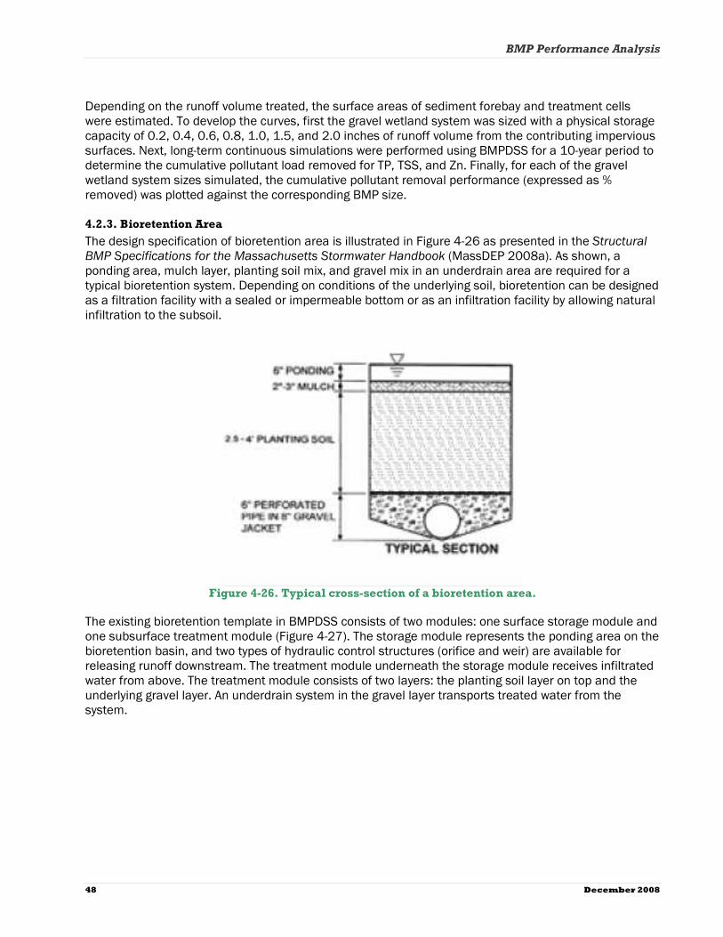
BMP Performance Analysis
48 December 2008
Depending on the runoff volume treated, the surface areas of sediment forebay and treatment cells were estimated. To develop the curves, first the gravel wetland system was sized with a physical storage capacity of 0.2, 0.4, 0.6, 0.8, 1.0, 1.5, and 2.0 inches of runoff volume from the contributing impervious surfaces. Next, long-term continuous simulations were performed using BMPDSS for a 10-year period to determine the cumulative pollutant load removed for TP, TSS, and Zn. Finally, for each of the gravel wetland system sizes simulated, the cumulative pollutant removal performance (expressed as % removed) was plotted against the corresponding BMP size.
4.2.3. Bioretention Area
The design specification of bioretention area is illustrated in Figure 4-26 as presented in the Structural BMP Specifications for the Massachusetts Stormwater Handbook (MassDEP 2008a). As shown, a ponding area, mulch layer, planting soil mix, and gravel mix in an underdrain area are required for a typical bioretention system. Depending on conditions of the underlying soil, bioretention can be designed as a filtration facility with a sealed or impermeable bottom or as an infiltration facility by allowing natural infiltration to the subsoil.
Figure 4-26. Typical cross-section of a bioretention area.
The existing bioretention template in BMPDSS consists of two modules: one surface storage module and one subsurface treatment module (Figure 4-27). The storage module represents the ponding area on the bioretention basin, and two types of hydraulic control structures (orifice and weir) are available for releasing runoff downstream. The treatment module underneath the storage module receives infiltrated water from above. The treatment module consists of two layers: the planting soil layer on top and the underlying gravel layer. An underdrain system in the gravel layer transports treated water from the system.
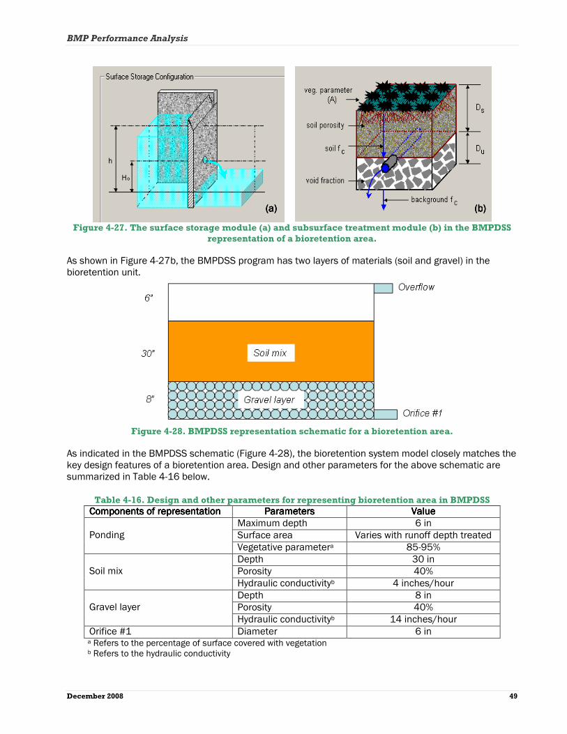
BMP Performance Analysis
December 2008 49
Figure 4-27. The surface storage module (a) and subsurface treatment module (b) in the BMPDSS
representation of a bioretention area.
As shown in Figure 4-27b, the BMPDSS program has two layers of materials (soil and gravel) in the bioretention unit.
Figure 4-28. BMPDSS representation schematic for a bioretention area.
As indicated in the BMPDSS schematic (Figure 4-28), the bioretention system model closely matches the key design features of a bioretention area. Design and other parameters for the above schematic are summarized in Table 4-16 below.
Table 4-16. Design and other parameters for representing bioretention area in BMPDSS
Components of representationComponents of representationComponents of representationComponents of representation ParametParametParametParametersersersers ValueValueValueValue Maximum depth 6 in Surface area Varies with runoff depth treated Ponding Vegetative parametera 85-95% Depth 30 in Porosity 40% Soil mix Hydraulic conductivityb 4 inches/hour Depth 8 in Porosity 40% Gravel layer Hydraulic conductivityb 14 inches/hour
Orifice #1 Diameter 6 in a Refers to the percentage of surface covered with vegetation b Refers to the hydraulic conductivity
(a)(a)(a)(a) ((((bbbb))))
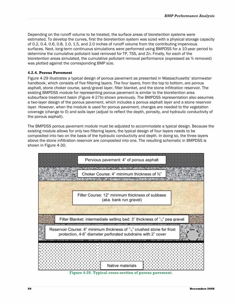
BMP Performance Analysis
50 December 2008
Depending on the runoff volume to be treated, the surface areas of bioretention systems were estimated. To develop the curves, first the bioretention system was sized with a physical storage capacity of 0.2, 0.4, 0.6, 0.8, 1.0, 1.5, and 2.0 inches of runoff volume from the contributing impervious surfaces. Next, long-term continuous simulations were performed using BMPDSS for a 10-year period to determine the cumulative pollutant load removed for TP, TSS, and Zn. Finally, for each of the bioretention areas simulated, the cumulative pollutant removal performance (expressed as % removed) was plotted against the corresponding BMP size.
4.2.4. Porous Pavement
Figure 4-29 illustrates a typical design of porous pavement as presented in Massachusetts’ stormwater handbook, which consists of five filtering layers. The four layers, from the top to bottom, are porous asphalt, stone choker course, sand/gravel layer, filter blanket, and the stone infiltration reservoir. The existing BMPDSS module for representing porous pavement is similar to the bioretention area subsurface treatment basin (Figure 4-27b) shown previously. The BMPDSS representation also assumes a two-layer design of the porous pavement, which includes a porous asphalt layer and a stone reservoir layer. However, when the module is used for porous pavement, changes are needed to the vegetation coverage (change to 0) and soils layer (adjust to reflect the depth, porosity, and hydraulic conductivity of the porous asphalt). The BMPDSS porous pavement module must be adjusted to accommodate a typical design. Because the existing module allows for only two filtering layers, the typical design of four layers needs to be composited into two on the basis of the hydraulic conductivity and depth. In doing so, the three layers above the stone infiltration reservoir are composited into one. The resulting schematic in BMPDSS is shown in Figure 4-30.
Figure 4-29. Typical cross-section of porous pavement.

BMP Performance Analysis
December 2008 51
Figure 4-30. The BMPDSS representation schematic for porous pavement design.
To accurately reflect the combined effects of the top three layers in typical design, principles depicting flow through multiple layers (Hillel 1998) were followed to generate the effective hydraulic conductivity for the composite layer in Figure 4-30. A list of the input parameters to complete the representation is summarized in Table 4-17.
Table 4-17. Design parameters for representing porous pavement in BMPDSS
Components of representationComponents of representationComponents of representationComponents of representation Design parametersDesign parametersDesign parametersDesign parameters ValueValueValueValue Depth 4 in Porosity 18–20% Porous asphalt Hydraulic conductivity 750 in/hr Depth 4 in Porosity 40% Chocker course Hydraulic conductivity 14 in/hr Depth 12–32 in Porosity 25%
Composite layer
Filter course Hydraulic conductivity 1.4 in/hr Depth 8 in Porosity 40% Gravel layer Hydraulic conductivity 14 in/hr
Porous pavement treats all the rainfall falls on it. It is impossible to size this BMP to treat a selected depth of runoff. In order to meet the transportation and other requirements, porous pavement needs to meet specific design standards. Four different sizes of porous pavement (by varying the thickness of the filter course), 12 (MA minimum requirement), 18, 24, 32 inches (UNHSC design standard) were used to develop the performance curves for this BMP.
Composite layer
Gravel layer
Bottom soil

BMP Performance Analysis
52 December 2008
4.2.5. Water Quality Swales
Water quality swales are vegetated open channels designed to treat the required water quality volume and to convey runoff from large storms. According to Massachusetts’ stormwater handbook, there are two different types of water quality swales that may be used to satisfy the state’s stormwater management standards; dry swales and wet swales. Although the design, construction, and processes for these swales differ, both types of swales perform similarly in pollutant removal (MassDEP 2008a). A typical water quality wet swale is illustrated in Figure 4-31. Wet swales store the water quality volume in a series of cells within the channel, which can be formed by berms or check dams and can contain wetland vegetation. The pollutant removal mechanisms in wet swales are similar to those of stormwater wetlands, which rely on sedimentation, adsorption, and microbial breakdown (MassDEP 2008a).
Figure 4-31. Typical design of a water quality wet swale.
The BMPDSS grass swale template consists of three components. The first component is the transport module (Figure 4-32), which routes stormwater flow through the grass swale channel. The second module (storage module) retains the water quality volume. It is similar to the surface storage module for a bioretention system as shown in Figure 4-27a. The third module is the subsurface infiltration module, which is similar to the subsurface treatment module for the bioretention area shown in Figure 4-27b. When used for the grass swale infiltration, the two-layer module shown in Figure 4-27b must be consolidated to one layer (eliminating the gravel layer). A list of the design parameters required to represent water quality swale is summarized in Table 4-18.
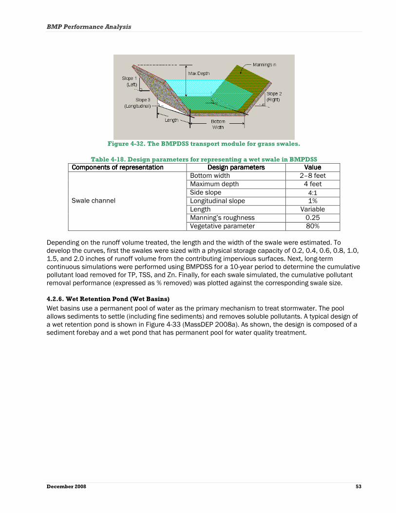
BMP Performance Analysis
December 2008 53
Figure 4-32. The BMPDSS transport module for grass swales.
Table 4-18. Design parameters for representing a wet swale in BMPDSS
Components of representationComponents of representationComponents of representationComponents of representation Design parametersDesign parametersDesign parametersDesign parameters ValueValueValueValue Bottom width 2–8 feet Maximum depth 4 feet Side slope 4:1 Longitudinal slope 1% Length Variable Manning’s roughness 0.25
Swale channel
Vegetative parameter 80% Depending on the runoff volume treated, the length and the width of the swale were estimated. To develop the curves, first the swales were sized with a physical storage capacity of 0.2, 0.4, 0.6, 0.8, 1.0, 1.5, and 2.0 inches of runoff volume from the contributing impervious surfaces. Next, long-term continuous simulations were performed using BMPDSS for a 10-year period to determine the cumulative pollutant load removed for TP, TSS, and Zn. Finally, for each swale simulated, the cumulative pollutant removal performance (expressed as % removed) was plotted against the corresponding swale size.
4.2.6. Wet Retention Pond (Wet Basins)
Wet basins use a permanent pool of water as the primary mechanism to treat stormwater. The pool allows sediments to settle (including fine sediments) and removes soluble pollutants. A typical design of a wet retention pond is shown in Figure 4-33 (MassDEP 2008a). As shown, the design is composed of a sediment forebay and a wet pond that has permanent pool for water quality treatment.
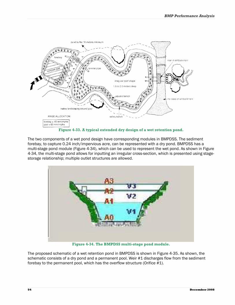
BMP Performance Analysis
54 December 2008
Figure 4-33. A typical extended dry design of a wet retention pond.
The two components of a wet pond design have corresponding modules in BMPDSS. The sediment forebay, to capture 0.24 inch/impervious acre, can be represented with a dry pond. BMPDSS has a multi-stage pond module (Figure 4-34), which can be used to represent the wet pond. As shown in Figure 4-34, the multi-stage pond allows for inputting an irregular cross-section, which is presented using stage-storage relationship; multiple outlet structures are allowed.
Figure 4-34. The BMPDSS multi-stage pond module.
The proposed schematic of a wet retention pond in BMPDSS is shown in Figure 4-35. As shown, the schematic consists of a dry pond and a permanent pool. Weir #1 discharges flow from the sediment forebay to the permanent pool, which has the overflow structure (Orifice #1).

BMP Performance Analysis
December 2008 55
Figure 4-35. BMPDSS representation schematic for wet retention pond design.
Depending on the runoff volume treated, the surface area of permanent pool is estimated. It is assumed the permanent pool has a depth of 6 feet and a side slope of 4:1 as Horizontal:Veritcal. Sediment forebay volume will be 0.25 times the permanent pool volume. According to the Massachusetts standards, this volume is excluded from the treatment volume. A list of the design parameters for the schematic is summarized in Table 4-19.
Table 4-19. Design parameters for representing a wet retention pond in BMPDSS
Components of representationComponents of representationComponents of representationComponents of representation Design parametersDesign parametersDesign parametersDesign parameters ValueValueValueValue Bottom area Variable Maximum depth 2 feet
Sediment forebay (Volume = 0.25 × Permanent Pool & Slope 4:1) Surface area Variable
Bottom area Variable Maximum depth 6 feet
Permanent Pool (Volume = Runoff Depth Treated × Area Treated & Slope 4:1) Surface area Variable
To develop the curves, the wet ponds were first sized with a physical storage capacity of 0.2, 0.4, 0.6, 0.8, 1.0, 1.5, and 2.0 inches of runoff volume from the contributing impervious surfaces. Next, long-term continuous simulations were performed using BMPDSS for a 10-year period to determine the cumulative pollutant load removed for TP, TSS, and Zn. Finally, for each wet pond size simulated, the cumulative pollutant removal performance (expressed as % removed) was plotted against the corresponding BMP size.
4.2.7. Extended Dry Detention (Dry Basins)
Extended dry detention basins are modified conventional dry detention basins designed to hold stormwater for at least 24 hours, allowing solids to settle and reducing local and downstream flooding. Extended dry detention basins can be designed with either a fixed or adjustable outflow device. Other components such as a micropool or shallow marsh can be added to enhance pollutant removal. A typical extended dry detention design is presented in Figure 4-36.

BMP Performance Analysis
56 December 2008
Figure 4-36. A typical design of an extended dry detention pond.
The proposed schematic of an extended dry detention pond in BMPDSS is shown in Figure 4-37. As shown, the representation consists of a dry pond and a permanent pool. Weir #1 discharges flow from the sediment forebay to detention basin, which has the overflow structure (Orifice #1) and discharge orifice (Orifice #2). The discharge orifice is sized to store the design volume and discharge in 24 hours. The sediment forebay, to capture 0.24 inches/impervious acre, can be represented with a dry pond.
Figure 4-37. BMPDSS representation schematic for extended dry detention pond design.

BMP Performance Analysis
December 2008 57
Depending on the runoff volume treated, the surface area of detention basin is estimated. It is assumed that the detention basin has a depth of 6 feet and a side slope of 4:1 as Horizontal:Vertical. Sediment forebay volume will be 0.25 times of permanent pool volume. According to the Massachusetts standards, this volume is excluded from the treatment volume. A list of the design parameters for the schematic is summarized in Table 4-20.
Table 4-20. Design parameters for representing extended dry detention pond in BMPDSS
Components of representationComponents of representationComponents of representationComponents of representation Design parametersDesign parametersDesign parametersDesign parameters ValueValueValueValue Bottom area Variable Maximum depth 2 feet
Sediment forebay (Volume = 0.25 × Permanent Pool & Slope 4:1) Surface area Variable
Bottom area (length: width = 2:1)
Variable
Maximum depth 6 feet
Detention basin (Volume = Runoff Depth Treated × Area Treated & Slope 4:1)
Surface area Variable To develop the curves, the extended dry ponds were first sized with a physical storage capacity of 0.2, 0.4, 0.6, 0.8, 1.0, 1.5, and 2.0 inches of runoff volume from the contributing impervious surfaces. Next, long-term continuous simulations were performed using BMPDSS for a 10-year period to determine the cumulative pollutant load removed for TP, TSS, and Zn. Finally, for each pond size simulated, the cumulative pollutant removal performance (expressed as % removed) was plotted against the corresponding BMP size.

BMP Performance Analysis
58 December 2008
5. PERFORMANCE CURVE
The calibrated BMPDSS model was applied for the following eight types of stormwater BMP to generate estimates of long-term cumulative BMP performances:
1. Surface infiltration systems (e.g., basin)
2. Subsurface infiltration systems (e.g., trench)
3. Gravel wetland systems
4. Bioretention systems
5. Water quality swales
6. Porous pavement systems
7. Wet ponds
8. Extended dry detention ponds Long-term BMP performance estimates for each BMP were generated for pollutant loading rates associated with each of the five land uses selected for the project (Commercial, Low-Density Residential, Medium-Density Residential, High-Density Residential, and Industrial). Long-term cumulative BMP performance estimates are presented as performance curves for each of the three water quality constituents, TP, TSS, and Zn. Performance curves were not generated for TN because there were insufficient TN monitoring data available for the BMPs during model calibration. Additionally, performance curves of runoff volume captured (runoff volume reduction) were generated for both the surface and subsurface infiltration systems. The runoff capture performance curves can be used to estimate change in effective impervious cover for limited circumstances. These curves will be equivalent to percent reduction in effective impervious area only in terms of annual runoff volume reductions. The performance curves are intended to be used to estimate long-term cumulative pollutant removal efficiencies (or runoff volume for infiltration systems) for BMPs that are based on similar design standards and according to the size (i.e., capacity) of the BMP system. Section 5.1 presents the concept of BMP performance curves, how they can be applied, and the assumptions and limitations of employing them.
5.1. BMP Performance Curve and Application
A series of BMP performance rating curves were developed for five land uses through the linkage of water quality and BMP models. Each BMP rating curve depicts the relationship between the size of a BMP and the percentage of pollutant removal over a long period of time (i.e., 10 years). The rating curves will help the practitioners to size BMPs for achieving known pollutant reduction goals or for determining appropriate pollutant removal credits for existing BMPs of known size. An example rating curve for gravel wetland performance in commercial land use is shown in Figure 5-1. The X axis is the size of the gravel wetland, represented by the depth (volume) of runoff to be treated by the gravel wetland. The Y axis is the long-term cumulative pollutant removal performance expressed as percent reduction. The rating curve shown in Figure 5-1 can be used for sizing BMPs depending on the objectives of pollutant removal. For example, if a target of 60 percent TP removal is sought for the gravel wetland system in Figure 5-1, a horizontal line can be drawn from the 60 percent value on the Y axis to the point where it intersects the TP performance curve. The vertical line drawn from the point on the TP curve intersects the X axis at
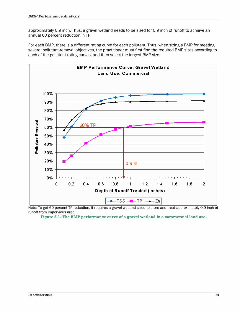
BMP Performance Analysis
December 2008 59
approximately 0.9 inch. Thus, a gravel wetland needs to be sized for 0.9 inch of runoff to achieve an annual 60 percent reduction in TP. For each BMP, there is a different rating curve for each pollutant. Thus, when sizing a BMP for meeting several pollutant-removal objectives, the practitioner must first find the required BMP sizes according to each of the pollutant-rating curves, and then select the largest BMP size.
Note: To get 60 percent TP reduction, it requires a gravel wetland sized to store and treat approximately 0.9 inch of runoff from impervious area.
Figure 5-1. The BMP performance curve of a gravel wetland in a commercial land use.

BMP Performance Analysis
60 December 2008
5.2. Example Application of BMP Performance Curve
One commercial site and one low-density residential site were selected to demonstrate how the BMP performance curves could be applied. Although the sites are real, the application is hypothetical. The demonstrated application below assumes that there are no existing BMPs.
5.2.1. Commercial Application
Site Details: Total Area = 40 acres, Total Impervious Area = 21 acres Location: Town of Bellingham, MA BMP Treatment Objective: 65 percent reduction of TP Site Overview: The site has two impervious sections. The upper section includes a small building, roads, and parking lots at the upper portion of the property boundary. The lower section includes the large building complex, roads, and parking lots. The upper section has imperviousness of approximately 2 acres and the lower section has approximately 19 acres. Assumptions: Soil infiltration rate = 0.52 in/hr, High groundwater depth = 10 ft This sample site is shown in Figure 5-2.

BMP Performance Analysis
December 2008 61
Figure 5-2. A sample commercial lot requires 65 percent TP reduction.

BMP Performance Analysis
62 December 2008
BMP Selection Among the BMPs for which performance information was generated, the wet pond, dry detention pond, and water quality swale were unsuitable for this site because the maximum TP removals are less than 65 percent. However, the gravel wetland and infiltration trench were identified as suitable options. Gravel wetlandGravel wetlandGravel wetlandGravel wetland Figure 5-3 illustrates the rating curve for a gravel wetland BMP in a commercial site.
Figure 5-3. BMP performance curve of gravel wetland in commercial land use.
To obtain 65 percent TP reduction, 1.5 inches of runoff from impervious surface needs to be stored and treated in a gravel wetland. Storage of the upper section gravel wetland = 1.5 in × 2 acres = 0.25 ac-ft Storage of the lower section = 1.5 in × 19 acres = 2.375 ac-ft Table 5-1 lists the design parameters for the gravel wetlands to reduce TP by 65 percent at the selected commercial site.

BMP Performance Analysis
December 2008 63
Table 5-1. Design parameters for potential gravel wetlands to reduce TP by 65 percent at the
commercial site.
Components of representationComponents of representationComponents of representationComponents of representation Design parametersDesign parametersDesign parametersDesign parameters Upper gravel Upper gravel Upper gravel Upper gravel wetlandwetlandwetlandwetland
Lower gravel Lower gravel Lower gravel Lower gravel wetlandwetlandwetlandwetland
Depth (in) 16 16 Sediment Forebay (10% of Treatment Volume) Surface area (sq. ft) 817 7,760
Surface area (sq. ft) 1,750 16,630 Ponding area
Depth (in) 24 24 Wetland Cell #1 (45% of Treatment Volume) Gravel layer (porosity =
0.4) Depth (in)
24 24
Surface area (sq. ft) 1,750 16,630 Ponding area
Depth (in) 24 24 Wetland Cell #2 (45% of Treatment Volume) Gravel layer
(porosity = 0.4) Depth (in)
24 24
Note: The selected BMP also provides approximately 99 percent reduction in TSS and 90 percent reduction in Zn from the impervious area. Option Option Option Option 2222: : : : Infiltration TrenchInfiltration TrenchInfiltration TrenchInfiltration Trench Figure 5-4 illustrates the rating curve for an infiltration trench BMP in a commercial land use.
Figure 5-4. BMP performance curve of an infiltration trench in a commercial land use (soil
infiltration rate is 0.52 in/hr).

BMP Performance Analysis
64 December 2008
For an infiltration trench, the Massachusetts stormwater specifications require pretreatment. This estimation assumes that the pretreatments are designed appropriately. To obtain 65 percent TP reduction, the trench system needs to have a storage capacity of 0.4 inch of runoff from impervious surfaces. These design parameters are listed in Table 5-2. Storage of the upper section infiltration basin = 0.4 in × 2 acres = 0.07 ac-ft Storage of the lower section = 0.4 in × 19 acres = 0.63 ac-ft
Table 5-2. Design parameters for the potential infiltration trenches to reduce TP by 65 percent at
the commercial site.
Components of representationComponents of representationComponents of representationComponents of representation Design parametersDesign parametersDesign parametersDesign parameters ValueValueValueValue Porosity 0.40
Sand filter Depth 6 in Depth 6 feet
Infiltration trench Stone layer
Porosity 0.45 Upper Infiltration Trench 1,010
Surface area (sq. ft) Upper Infiltration Trench 9,470
Note: The selected infiltration trench also provides approximately 98 percent reduction in Zn, 90 percent reduction in TSS and 60 percent reduction in runoff volume from the impervious area.
5.2.2. Low-Density Residential Application
Site Details: Total Area = 1.3 acres, Total Impervious Area = 0.4 acres Location: Town of Milford, MA BMP Treatment Objective: 65 percent reduction of TP Site Overview: The site has a building and driveway as impervious area. Assumptions: Soil infiltration rate = 0.27 in/hr, High groundwater depth = 10 ft This sample site is shown in Figure 5-5.

BMP Performance Analysis
December 2008 65
Figure 5-5. A sample Low-Density residential lot requires 65 percent TP reduction.
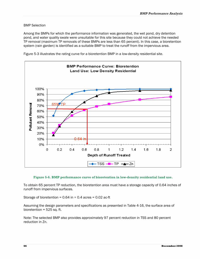
BMP Performance Analysis
66 December 2008
BMP Selection Among the BMPs for which the performance information was generated, the wet pond, dry detention pond, and water quality swale were unsuitable for this site because they could not achieve the needed TP removal (maximum TP removals of these BMPs are less than 65 percent). In this case, a bioretention system (rain garden) is identified as a suitable BMP to treat the runoff from the impervious area. Figure 5-3 illustrates the rating curve for a bioretention BMP in a low-density residential site.
Figure 5-6. BMP performance curve of bioretention in low-density residential land use.
To obtain 65 percent TP reduction, the bioretention area must have a storage capacity of 0.64 inches of runoff from impervious surfaces. Storage of bioretention = 0.64 in × 0.4 acres = 0.02 ac-ft Assuming the design parameters and specifications as presented in Table 4-16, the surface area of bioretention = 525 sq. ft. Note: The selected BMP also provides approximately 97 percent reduction in TSS and 80 percent reduction in Zn.

BMP Performance Analysis
December 2008 67
5.3. Assumptions and Limitations
BMP performance curves developed and reported here rely on the modeling of real BMP systems. Calibrated land-based and BMP models were used to simulate hydrologic and water quality processes for both the land and BMP components. All assumptions of the models that were used—SWMM (Huber and Dickinson 1988) for land simulation and BMPDSS (Tetra Tech 2005a) for BMP simulation—are applicable to this study. Another major assumption is that the BMPs are appropriately designed, built, and maintained as required by Massachusetts stormwater requirements presented in the Structural BMP Specifications for the Massachusetts Stormwater Handbook (MassDEP 2008a). The following is the summary of assumptions and limitations for developing and applying BMP performance curves that were created for this project.
• BMP configuration and placement:
o The curves represent the pollutant removal performance of each BMP as an independent unit. It would be inappropriate to use these curves directly if BMPs were to be installed in series.
o Another assumption and limitation is that the BMP performance curves were developed to treat stormwater runoff from impervious surfaces. Thus, it would be inappropriate to use these curves directly to size BMPs to treat runoff from pervious surfaces. However, if a system were designed to treat runoff from an area that includes both impervious and pervious areas, the size of the BMP should account for any runoff volume that could be contributed by the pervious area. This should not be an issue if the BMP size is less than the initial abstraction for the pervious area because the pervious area should not contribute runoff for storms less than this size. However, if, for example, the BMP were sized to treat 1 inch of runoff from impervious area and the drainage area includes pervious area with an initial abstraction of 0.7 inches, the actual size of the BMP capacity would need to be increased by 0.3 inch from the pervious area to obtain full reduction credit for treating the impervious area.
• BMP performance and applicability
o Operation and maintenance of BMPs are performed according to the specifications and, therefore, BMPs maintain the same performance during their life time.
o Soil characteristics of BMP sites remain the same over the BMPs’ life time.
o BMP performance curves were developed using the precipitation records from Boston, Massachusetts. It would be appropriate to use the curves for other regions with similar precipitation characteristics. The use of these curves beyond the precipitation characteristics of Boston, Massachusetts, would require further examination.
The benefits of the system of developed BMP performance curves are much more than its limitations. The system provides a quick assessment tool targeted to the New England region that can be used to evaluate selected BMP siting to meet a range of reduction targets for specific pollutants. The direct use of the system of curves saves resources required for detailed modeling and other evaluations for each site. The system of curves also can be used to quantify the credits associated with existing BMPs. The system can be used to evaluate the alternatives of BMPs for mitigating the effects of development and benefits of redevelopment.

BMP Performance Analysis
68 December 2008
ACKNOWLEDGEMENTS
The authors of this report and primary investigators of the study, Tham Saravanapavan and Guoshun Zhang, would like to acknowledge Mark Voorhees, Work Assignment Manager (WAM), of the U.S. Environmental Protection Agency for his continued guidance and support throughout the study. The authors express gratitude to the study collaborators, Professor Robert Roseen and James Houle of the University of New Hampshire Stormwater Center. At the beginning of the study, the EPA WAM formed a technical advisory committee (TAC). The TAC met five times at EPA, Boston, Massachusetts, and convened on conference calls during the study period to provide Tetra Tech continued support. The TAC includes the following members:
1. Mark Voorhees, U.S. Environmental Protection Agency 2. Stephen Silva, U.S. Environmental Protection Agency 3. David Webster, U.S. Environmental Protection Agency 4. David Gray, U.S. Environmental Protection Agency 5. Eric Perkins, U.S. Environmental Protection Agency 6. Holly Galavotti, U.S. Environmental Protection Agency 7. Jennie Bridge, U.S. Environmental Protection Agency 8. John Smaldone, U.S. Environmental Protection Agency 9. Thelma Murphy, U.S. Environmental Protection Agency 10. Maggie Theroux, U.S. Environmental Protection Agency 11. Todd Borci, U.S. Environmental Protection Agency 12. William Walshrogalski, U.S. Environmental Protection Agency 13. Dennis Dunn, Massachusetts Department of Environmental Protection 14. David C. Noonan, Massachusetts Department of Environmental Protection 15. Frederick Civian, Massachusetts Department of Environmental Protection 16. Paul Hogan. Massachusetts Department of Environmental Protection 17. Christopher Bellucci, Connecticut Department of Environmental Protection 18. Robert Roseen, University of New Hampshire 19. Tham Saravanapavan, Tetra Tech, Inc.
The authors thank the members of the TAC for their support provided at every step of the study. The authors also acknowledge Dr. Mow-Soung Cheng, Prince George’s County, Maryland and Leslie Shoemaker, Greg Mallon, Andrew Parker, Jenny Zhen, Khalid Alvi, and Jeff Strong of Tetra Tech, Inc., for their support in this study.

December 2008 69
REFERENCES
Behera, P.K., B.J. Adams, and J.Y. Li. 2006. Runoff quality analysis of urban catchments with analytical probabilistic models. Journal of Water Resources Planning and Management 132(1):4–14.
Hillel, D. 1998. Environmental Soil Physics. Academic Press, San Diego, CA:.
Huber, W.C., and R.E. Dickinson. 1988. Storm Water Management Model Version 4, User’s Manual. EPA/600/3-88/001a (NTIS PB88-236641/AS), U.S. Environmental Protection Agency, Athens, GA.
MassDEP (Massachusetts Department of Environmental Protection). 2008a. Structural BMP Specifications for the Massachusetts Stormwater Handbook. Volume 2, Chapter 2. Massachusetts Department of Environmental Protection, Worcester, MA.
MassDEP (Massachusetts Department of Environmental Protection). 2008b. Documenting Compliance with the Massachusetts Stormwater Management Standards. Volume 3, Chapter 1. Massachusetts Department of Environmental Protection, Worcester, MA.
MassDEP (Massachusetts Department of Environmental Protection) and USEPA (U.S. Environmental Protection Agency). 2007. Total Maximum Daily Load for Lower Charles River Basin, Massachusetts. Massachusetts Department of Environmental Protection, Worcester, MA, and U.S. Environmental Protection Agency, Boston, MA.
Rossman, L.A. 2007. Stormwater Management Model User’s Manual, Version 5.0. EPA/600/R-05/040. U.S. Environmental Protection Agency, National Risk Management Research Laboratory, Cincinnati, OH.
Shaver, E., R.Horner, J. Skupien, C.May, and G. Ridley. 2007. Fundamentals of Urban Runoff Management: Technical and Institutional Issues. 2nd ed. North American Lake Management Society, Madison, WI.
Tetra Tech. 2007. Prince George’s County BMPDSS Calibration/Validation using Field Monitoring Data. Prepared for Prince George’s County, Department of Environmental Resources, by Tetra Tech, Inc., Fairfax, VA.
Tetra Tech. 2005a. BMP/LID Decision Support System for Watershed-Based Stormwater Management: Users Guide. Prepared for Prince George’s County, Department of Environmental Resources, by Tetra Tech, Inc., Fairfax, VA.
Tetra Tech. 2005b. BMP/LID Decision Support System for Watershed-Based Stormwater Management: Step-by-Step Application Guide. Prepared for Prince George’s County, Department of Environmental Resources, by Tetra Tech, Inc., Fairfax, VA.
UNHSC (University of New Hampshire Stormwater Center). 2007. 2007 Annual Report. University of New Hampshire Stormwater Center, Durham, NH.

BMP Performance Analysis
70 December 2008
USDA-NRCS (U.S. Department of Agriculture—Natural Resources Conservation Service). 1986. Urban Hydrology for Small Watersheds, TR-55. U.S. Department of Agriculture—Natural Resources Conservation Service, Washington, DC.
USEPA (U.S. Environmental Protection Agency). 1999. Stormater Technology Fact Sheet: Bio-retention. EPA 832-F-99-012. U.S. Environmental Protection Agency Office of Water, Washington, DC.
Walker, W.W., Jr. 1990. P8 urban catchment model program documentation, v1.1. Prepared for IEP, Inc., Northborough, MA and Narragansett Bay Project, Providence, RI.

December 2008 71
APPENDIX A:
BACKGROUND ON BMPDSS
A.1. Land Use Time Series
In BMPDSS, hydrographs and pollutographs from the drainage area are routed through BMPs placed in the project area. To simplify the land simulation process, land use-based hydrographs and pollutographs are developed using watershed model and stored in the database. For example, Hydrologic Simulation Program, FORTRAN (HSPF) was applied to generate the time series in the Prince George’s County version of BMPDSS. The BMP performance analysis for New England employs SWMM (as detailed in section 3 of this report) for generating hydrographs and pollutographs for the selected land uses and stored in the geospatial database.
A.2. BMPDSS
Jurisdictions with established urban areas and newly developing areas must find cost-effective means for minimizing effects of development and for planning future growth. BMPDSS can be applied to analyze the overall performance of multiple BMPs and find an optimal solution for their implementation. BMPDSS can provide assessment of both distributed (including LID-type) and centralized BMPs in combinations implemented for a given watershed management or TMDL implementation plan and can support selection of the optimum plan that maximizes benefits and leads to significant cost savings. This quantitative approach can provide assurance to stormwater managers and regulators that goals or TMDL reduction requirements are achievable and practicable, thereby ensuring that investments in selected BMPs are justified. The BMPDSS is a decision-making tool for placing BMPs at strategic locations in urban watersheds on the basis of integrated data collection and hydrologic, hydraulic, and water quality modeling. The key questions that can be addressed by the analysis system are as follows:
1. What is the benefit of management? 2. What is the difference between management options/scenarios including one or more practices? 3. What is the cost? That is, what is the difference in cost versus the measures of benefit described
in questions 1 and 2? The potential users of this system include local and county government planners; state, and federal regulatory reviewers; public concerned citizen/stakeholder groups; private industry; consultants; and academics. The system uses GIS information and technology and time series data for watershed runoff flow and pollutant concentration (generated by the watershed model), integrates BMP process simulation models, and applies system optimization techniques for BMP planning and selection. ESRI ArcGIS is employed as the system platform to provide GIS-based visualization and support for developing networks that include sequences of land uses, BMPs, and stream reaches. The system also provides interfaces for BMP placement, BMP attribute data input, and decision optimization management. The system includes a standalone BMP simulation and evaluation module, which complements both research and regulatory stormwater control assessment efforts and allows flexibility in examining various BMP design alternatives. Process-based simulation of BMPs provides a technique that is sensitive to local climate and rainfall patterns. The routing simulation component routes the flow and water quality constituents

BMP Performance Analysis
72 December 2008
through the conveyance network. The system also incorporates a meta-heuristic optimization technique to find the most cost-effective BMP placement and implementation plan given a control target or a fixed cost.
ArcGIS Interface
The ArcGIS interface is the main user interface. It includes the main application window with menus, buttons, and dialog boxes. The interface is implemented in Visual Basic programming language with ArcObjects, and it requires two ArcGIS components—ArcView 9.x (ArcMap) and Spatial Analyst. The ArcGIS interface allows the user to read and edit the spatial and temporal data sets and interact with the database component of the system. The interface also provides a platform for BMP placement and configuration, delineating drainage area, and establishing a routing network.
BMP Simulation Module
The BMP simulation module uses process-based algorithms to simulate BMP function and removal efficiency and accepts flow and water quality time series (acquired through observation or generated by runoff models) as input data. Process-based algorithms include weir and orifice control structures, storm swale characteristics, flow and pollutant transport, flow routing and networking, infiltration and saturation, evapotranspiration, and a general loss/decay representation for a pollutant. BMP effectiveness can be evaluated and estimated over a wide range of storm conditions, site designs, and flow routing configuration approaches. The processes incorporated include the following:
• Infiltration • Orifice outflow • Controlled orifice release (the user can define an hourly outflow rate, and there is an on/off
switch) • Weir-controlled overflow spillway • Underdrain outflow • Bottom slope influence • Bottom roughness influence • General loss or decay of pollutant (due to settling, plant uptake, volatilization, and so forth) • Pollutant filtration through the soil medium (represented by underdrain outflow) • Evapotranspiration

December 2008 73
The major BMP types that can be represented in BMPDSS are storage-type devices (such as rain barrels, cisterns, and detention basins), bioretention basins, filters, and swales (Figure A-1).
Figure A-1. Available BMP options in BMPDSS.
Routing/Transport Module
Flow and pollutants are routed through the pipes or channels in a routing network with the user’s choice of cross section by using the Storm Water Management Model (SWMM) (version 5) transport algorithms. The SWMM-Transport module tracks the flow rate, flow depth, and quality of water in each pipe and channel during a simulation period. Water quality routing within conduit links assumes that the conduit behaves like a continuously stirred tank reactor (CSTR). The concentration of a constituent exiting the conduit at the end of a time step is found by integrating the conservation of mass equation, using average values for quantities that might change over the time step, such as flow rate and conduit volume. Input flows and pollutants loadings from external and dry-weather inflows are supplied through time series data associated with a junction of the conduit inlet.

BMP Performance Analysis
74 December 2008
Optimization Component
The optimization component provides evolutionary optimization techniques to identify the most cost-efficient BMP selection and placement strategies according to user-defined decision criteria, including assessment points (e.g., outfall locations) and evaluation factors (e.g., flow and water quality). The function of the optimization engine is to determine the locations, types, and design configurations of the BMPs that best satisfy the user-defined water quality, water quantity, or cost objectives within user-defined constraints. The system provides an evaluation factor pick-list from which the user can choose. In the current version (version 1.0), the following factors are provided:
• Water Quantity Evaluation Factors • Annual Average Flow Volume (AAFV) • Peak Discharge Flow (PDF) within simulation period • Flow Exceeding Frequency (FEF) for user-specified threshold rate • Water Quality Evaluation Factors (sediment and other user-specified pollutants)
o Annual Average Load (AAL) o Annual Average Concentration (AAC) o Maximum Moving Average Concentration (MAC) for a user-specified time period
Each evaluation factor can be presented in three modes: (1) percent of existing condition, (2) scaled between pre-developed and existing condition, and (3) value. As an important factor in optimization formulation, the cost function estimates the total costs of the BMP systems. BMPDSS includes a generic cost function to provide relationships between BMP cost and excavation volume; a linear, land-cost term is also included. The optimization component employs scatter search as the solution algorithm. Scatter search is a meta-heuristic search technique that has been explored and used in optimizing complex systems (Glover et al. 19991). The scatter search approach does not emphasize randomization, particularly in the sense of being indifferent to choices among alternatives. Instead, the approach is designed to incorporate strategic responses, both deterministic and probabilistic, that take evaluation and history into account. Scatter search focuses on generating relevant outcomes without losing the ability to produce diverse solutions because of the way the generation process is implemented (Laguna and Marti 20022). Because of this feature of scatter search, for optimization problems that have a CPU time-consuming evaluator, it is expected that scatter search can find the near-optimal solution more efficiently and serve as a better optimization engine.
Post-processor
To aid in the processing, analysis, and examination of output data produced by BMPDSS, a result analysis tool or post-processor has been incorporated into the system. The post-processor has two components. One is in the ArcGIS environment and is mainly for displaying the evaluation factor values for defined assessment points; the other is a Microsoft Excel spreadsheet with macros. The post-processor tool is designed to facilitate the evaluation of BMP/LID performance and to provide insights for the following assessment questions:
• What are the hydrologic and water quality impacts of a proposed or existing development site? • What is a reasonable pre-developed condition for the site? • How does the developed scenario compare with the pre-development condition?
1 Glover, F., M. Laguna, and R. Marti. 1999. Scatter Search to Appear in Theory and Applications of Evolutionary Computation: Recent Trends. Ed., A. Ghosh and S. Tsutsui. Springer-Verlag.
2 Laguna, M., and R. Marti. 2002. The OptQuest Callable Library to Appear in Optimization Software Class Libraries. Ed. S. Voss and D.L. Woodruff. Kluwer Academic Publishers, Boston. Pp. 193–218.
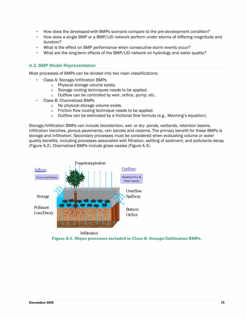
December 2008 75
• How does the developed-with-BMPs scenario compare to the pre-development condition? • How does a single BMP or a BMP/LID network perform under storms of differing magnitude and
duration? • What is the effect on BMP performance when consecutive storm events occur? • What are the long-term effects of the BMP/LID network on hydrology and water quality?
A.3. BMP Model Representation
Most processes of BMPs can be divided into two main classifications:
• Class A: Storage/Infiltration BMPs o Physical storage volume exists. o Storage routing techniques needs to be applied. o Outflow can be controlled by weir, orifice, pump, etc.
• Class B: Channelized BMPs o No physical storage volume exists. o Friction flow routing technique needs to be applied. o Outflow can be estimated by a frictional flow formula (e.g., Manning’s equation).
Storage/Infiltration BMPs can include bioretention, wet- or dry- ponds, wetlands, retention basins, infiltration trenches, porous pavements, rain barrels and cisterns. The primary benefit for these BMPs is storage and infiltration. Secondary processes must be considered when evaluating volume or water quality benefits, including processes associated with filtration, settling of sediment, and pollutants decay (Figure A-2). Channelized BMPs include grass swales (Figure A-3).
OverflowSpillway
Bottom Orifice
Evapotranspiration
Infiltration
Outflow:Inflow:
Modified Flow &Water Quality
From Land Surface
Storage
Pollutant Loss/Decay
Figure A-2. Major processes included in Class A: Storage/Infiltration BMPs.

BMP Performance Analysis
76 December 2008
Outflow:Inflow:
Modified Flow &
Water Qual ity
From Land Surface
Overflow atMax Design
Depth
Open Channel Flow
Evapotranspiration
Pollutant Loss/Decay
Infiltration Figure A-3. Major processes included in Class B: Channelized BMPs.
Key processes that affect BMP effectiveness include infiltration and pollutant removal. The BMP simulation module in BMPDSS employs Holtan-Lopez empirical model (Equation 1) to represent infiltration and evapotransporation during a storm event.
(1) In equation 1, f is the infiltration rate (in/hr); GI is the growth index of vegetation in percent maturity, varying from 0.1 to 1.0; A is the vegetative parameter that characterizes surface-connected porosity and the density of plant roots, which affect infiltration; Sa is the available storage in the surface layer (inches); and fc is the final constant infiltration rate (in/hr), which is a function of the infiltration capacity of the substrate.
The water quality simulation considers two mechanisms: general loss or decay of pollutant (because of settling, plant-uptake, volatilization, and so on); and pollutant filtration through substrate. The general loss or decay is represented using a first order decay model:
Ct = C0 e (-kt) (2)
where, Ct is the pollutant concentration at time t, C0 is the initial pollutant concentration, and k is the first order decay rate (T-1).
The pollutant filtration through substrate is simulated using percent removal:
Cud_out = Prem Cin e (-kt) / 100 (3)
where, Cud_out is the underdrain outflow pollutant concentration, Cin is pollutant concentration in inflow to the substrate, Prem is percent removal rate (%), and t is time (model simulation occurs at a 1-hour time-step).
f GI AS fa c= +1 4.

December 2008 77
Figure A-4 illustrates the water quality simulation processes that take place in a BMP.
Figure A-4. Water quality simulation processes.
APPENDIX B: BMP RERFORMANCE
CURVES
BMP Performance Curve: Infiltration Trench
Page 79
BMP Performance Curve: Infiltration
Trench
Prepared for: United States Environmental Protection Agency – Region 1 One Congress Street, Suite 1100 Boston, MA 02114 Prepared by: Tetra Tech, Inc. 10306 Eaton Place, Suite 340 Fairfax, VA 22030 September 2008
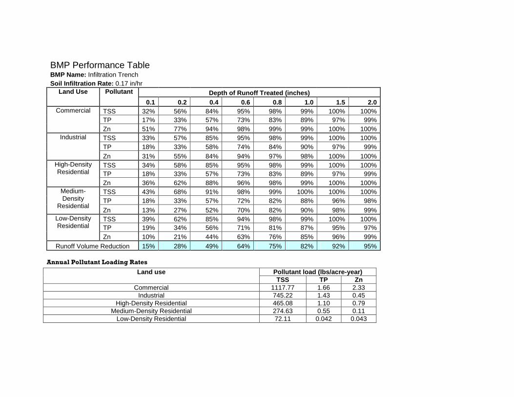
BMP Performance Table BMP Name: Infiltration Trench Soil Infiltration Rate: 0.17 in/hr
Depth of Runoff Treated (inches) Land Use Pollutant
0.1 0.2 0.4 0.6 0.8 1.0 1.5 2.0 TSS 32% 56% 84% 95% 98% 99% 100% 100% TP 17% 33% 57% 73% 83% 89% 97% 99%
Commercial
Zn 51% 77% 94% 98% 99% 99% 100% 100% TSS 33% 57% 85% 95% 98% 99% 100% 100% TP 18% 33% 58% 74% 84% 90% 97% 99%
Industrial
Zn 31% 55% 84% 94% 97% 98% 100% 100% TSS 34% 58% 85% 95% 98% 99% 100% 100% TP 18% 33% 57% 73% 83% 89% 97% 99%
High-Density Residential
Zn 36% 62% 88% 96% 98% 99% 100% 100% TSS 43% 68% 91% 98% 99% 100% 100% 100% TP 18% 33% 57% 72% 82% 88% 96% 98%
Medium-Density
Residential Zn 13% 27% 52% 70% 82% 90% 98% 99% TSS 39% 62% 85% 94% 98% 99% 100% 100% TP 19% 34% 56% 71% 81% 87% 95% 97%
Low-Density Residential
Zn 10% 21% 44% 63% 76% 85% 96% 99%
Runoff Volume Reduction 15% 28% 49% 64% 75% 82% 92% 95%
Annual Pollutant Loading Rates
Pollutant load (lbs/acre-year) Land use TSS TP Zn
Commercial 1117.77 1.66 2.33 Industrial 745.22 1.43 0.45
High-Density Residential 465.08 1.10 0.79 Medium-Density Residential 274.63 0.55 0.11
Low-Density Residential 72.11 0.042 0.043

BMP Performance Curve: Infiltration Trench
81
BMP Performance Curve: Infiltration TrenchLand Use: Commercial
(Soil infiltration rate 0.17 in/hr)
0%
10%
20%
30%
40%
50%
60%
70%
80%
90%
100%
0 0.2 0.4 0.6 0.8 1 1.2 1.4 1.6 1.8 2
Depth of Runoff Treated (inches)
Po
lluta
nt
Rem
ova
l
0%
10%
20%
30%
40%
50%
60%
70%
80%
90%
100%
Ru
no
ff V
olu
me
Red
uct
ion
TSS TP Zn Volume

82
BMP Performance Curve: Infiltration TrenchLand Use: Industrial
(Soil Infiltration Rate 0.17 in/hr)
0%
10%
20%
30%
40%
50%
60%
70%
80%
90%
100%
0 0.2 0.4 0.6 0.8 1 1.2 1.4 1.6 1.8 2
Depth of Runoff Treated (inches)
Po
lluta
nt R
emo
val
0%
10%
20%
30%
40%
50%
60%
70%
80%
90%
100%
Ru
no
ff V
olu
me
Red
uct
ion
TSS TP Zn Volume

BMP Performance Curve: Infiltration Trench
83
BMP Performance Curve: Infiltration TrenchLand Use: High Density Residential
(Soil infiltration rate 0.17 in/hr)
0%
10%
20%
30%
40%
50%
60%
70%
80%
90%
100%
0 0.2 0.4 0.6 0.8 1 1.2 1.4 1.6 1.8 2
Depth of Runoff Treated (inches)
Po
lltan
t R
emo
val
0%
10%
20%
30%
40%
50%
60%
70%
80%
90%
100%
Ru
no
ff V
olu
me
Red
uct
ion
TSS TP Zn Volume

84
BMP Performance Curve: Infiltration TrenchLand Use: Medium Density Residential
(Soil Infiltration Rate 0.17 in/hr)
0%
10%
20%
30%
40%
50%
60%
70%
80%
90%
100%
0 0.2 0.4 0.6 0.8 1 1.2 1.4 1.6 1.8 2
Depth of Runoff Treated
Po
lluta
nt
Rem
ova
l
0%
10%
20%
30%
40%
50%
60%
70%
80%
90%
100%
Ru
no
ff V
olu
me
Red
uct
ion
TSS TP Zn Volume

BMP Performance Curve: Infiltration Trench
85
BMP Performance Curve: Infiltration TrenchLand Use: Low Density Residential
(Soil Infiltration Rate 0.17 in/hr)
0%
10%
20%
30%
40%
50%
60%
70%
80%
90%
100%
0 0.2 0.4 0.6 0.8 1 1.2 1.4 1.6 1.8 2
Depth of Runoff Treated
Po
lluta
nt
Rem
ova
l
0%
10%
20%
30%
40%
50%
60%
70%
80%
90%
100%
Ru
no
ff V
olu
me
Red
uct
ion
TSS TP Zn Volume
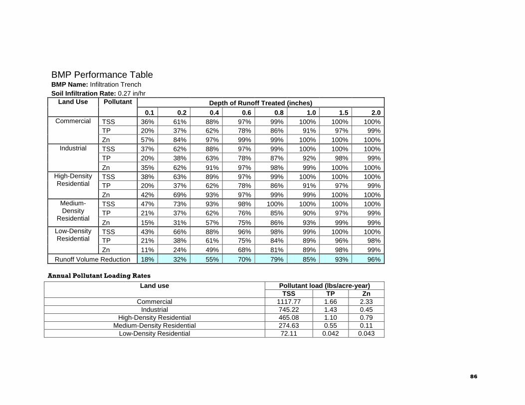
86
BMP Performance Table BMP Name: Infiltration Trench Soil Infiltration Rate: 0.27 in/hr
Depth of Runoff Treated (inches) Land Use Pollutant
0.1 0.2 0.4 0.6 0.8 1.0 1.5 2.0 TSS 36% 61% 88% 97% 99% 100% 100% 100% TP 20% 37% 62% 78% 86% 91% 97% 99%
Commercial
Zn 57% 84% 97% 99% 99% 100% 100% 100% TSS 37% 62% 88% 97% 99% 100% 100% 100% TP 20% 38% 63% 78% 87% 92% 98% 99%
Industrial
Zn 35% 62% 91% 97% 98% 99% 100% 100% TSS 38% 63% 89% 97% 99% 100% 100% 100% TP 20% 37% 62% 78% 86% 91% 97% 99%
High-Density Residential
Zn 42% 69% 93% 97% 99% 99% 100% 100% TSS 47% 73% 93% 98% 100% 100% 100% 100% TP 21% 37% 62% 76% 85% 90% 97% 99%
Medium-Density
Residential Zn 15% 31% 57% 75% 86% 93% 99% 99% TSS 43% 66% 88% 96% 98% 99% 100% 100% TP 21% 38% 61% 75% 84% 89% 96% 98%
Low-Density Residential
Zn 11% 24% 49% 68% 81% 89% 98% 99%
Runoff Volume Reduction 18% 32% 55% 70% 79% 85% 93% 96%
Annual Pollutant Loading Rates
Pollutant load (lbs/acre-year) Land use TSS TP Zn
Commercial 1117.77 1.66 2.33 Industrial 745.22 1.43 0.45
High-Density Residential 465.08 1.10 0.79 Medium-Density Residential 274.63 0.55 0.11
Low-Density Residential 72.11 0.042 0.043

BMP Performance Curve: Infiltration Trench
87
BMP Performance Curve: Infiltration TrenchLand Use: Commercial
(Soil infiltration rate 0.27 in/hr)
0%
10%
20%
30%
40%
50%
60%
70%
80%
90%
100%
0 0.2 0.4 0.6 0.8 1 1.2 1.4 1.6 1.8 2
Depth of Runoff Treated (inches)
Po
lluta
nt
Rem
ova
l
0%
10%
20%
30%
40%
50%
60%
70%
80%
90%
100%
Ru
no
ff V
olu
me
Red
uct
ion
TSS TP Zn Volume

88
BMP Performance Curve: Infiltration TrenchLand Use: Industrial
(Soil Infiltration Rate 0.27 in/hr)
0%
10%
20%
30%
40%
50%
60%
70%
80%
90%
100%
0 0.2 0.4 0.6 0.8 1 1.2 1.4 1.6 1.8 2
Depth of Runoff Treated (inches)
Po
lluta
nt R
emo
val
0%
10%
20%
30%
40%
50%
60%
70%
80%
90%
100%
Ru
no
ff V
olu
me
Red
uct
ion
TSS TP Zn Volume

BMP Performance Curve: Infiltration Trench
89
BMP Performance Curve: Infiltration TrenchLand Use: High Density Residential
(Soil infiltration rate 0.27 in/hr)
0%
10%
20%
30%
40%
50%
60%
70%
80%
90%
100%
0 0.2 0.4 0.6 0.8 1 1.2 1.4 1.6 1.8 2
Depth of Runoff Treated (inches)
Po
lltan
t R
emo
val
0%
10%
20%
30%
40%
50%
60%
70%
80%
90%
100%
Ru
no
ff V
olu
me
Red
uct
ion
TSS TP Zn Volume

90
BMP Performance Curve: Infiltration TrenchLand Use: Medium Density Residential
(Soil Infiltration Rate 0.27 in/hr)
0%
10%
20%
30%
40%
50%
60%
70%
80%
90%
100%
0 0.2 0.4 0.6 0.8 1 1.2 1.4 1.6 1.8 2
Depth of Runoff Treated
Po
lluta
nt
Rem
ova
l
0%
10%
20%
30%
40%
50%
60%
70%
80%
90%
100%
Ru
no
ff V
olu
me
Red
uct
ion
TSS TP Zn Volume
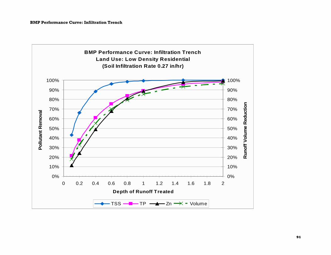
BMP Performance Curve: Infiltration Trench
91
BMP Performance Curve: Infiltration TrenchLand Use: Low Density Residential
(Soil Infiltration Rate 0.27 in/hr)
0%
10%
20%
30%
40%
50%
60%
70%
80%
90%
100%
0 0.2 0.4 0.6 0.8 1 1.2 1.4 1.6 1.8 2
Depth of Runoff Treated
Po
lluta
nt
Rem
ova
l
0%
10%
20%
30%
40%
50%
60%
70%
80%
90%
100%
Ru
no
ff V
olu
me
Red
uct
ion
TSS TP Zn Volume

92
BMP Performance Table BMP Name: Infiltration Trench Soil Infiltration Rate: 0.52 in/hr
Depth of Runoff Treated (inches) Land Use Pollutant
0.1 0.2 0.4 0.6 0.8 1.0 1.5 2.0 TSS 40% 66% 91% 98% 99% 100% 100% 100% TP 23% 42% 67% 82% 89% 94% 98% 99%
Commercial
Zn 65% 90% 98% 99% 100% 100% 100% 100% TSS 41% 67% 91% 98% 99% 100% 100% 100% TP 24% 42% 68% 82% 90% 94% 98% 99%
Industrial
Zn 41% 69% 92% 99% 99% 100% 100% 100% TSS 42% 68% 91% 98% 99% 100% 100% 100% TP 24% 42% 68% 82% 89% 94% 98% 99%
High-Density Residential
Zn 48% 77% 97% 99% 99% 100% 100% 100% TSS 52% 77% 95% 99% 100% 100% 100% 100% TP 24% 42% 67% 81% 88% 93% 97% 99%
Medium-Density
Residential Zn 18% 35% 63% 81% 91% 96% 100% 100% TSS 47% 70% 91% 97% 99% 100% 100% 100% TP 25% 43% 66% 80% 87% 92% 97% 98%
Low-Density Residential
Zn 13% 28% 55% 73% 85% 93% 99% 99%
Runoff Volume Reduction 22% 38% 62% 76% 84% 89% 95% 97%
Annual Pollutant Loading Rates
Pollutant load (lbs/acre-year) Land use TSS TP Zn
Commercial 1117.77 1.66 2.33 Industrial 745.22 1.43 0.45
High-Density Residential 465.08 1.10 0.79 Medium-Density Residential 274.63 0.55 0.11
Low-Density Residential 72.11 0.042 0.043
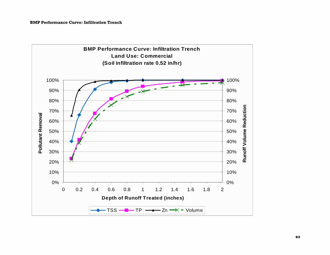
BMP Performance Curve: Infiltration Trench
93
BMP Performance Curve: Infiltration TrenchLand Use: Commercial
(Soil infiltration rate 0.52 in/hr)
0%
10%
20%
30%
40%
50%
60%
70%
80%
90%
100%
0 0.2 0.4 0.6 0.8 1 1.2 1.4 1.6 1.8 2
Depth of Runoff Treated (inches)
Po
lluta
nt
Rem
ova
l
0%
10%
20%
30%
40%
50%
60%
70%
80%
90%
100%
Ru
no
ff V
olu
me
Red
uct
ion
TSS TP Zn Volume

94
BMP Performance Curve: Infiltration TrenchLand Use: Industrial
(Soil Infiltration Rate 0.52 in/hr)
0%
10%
20%
30%
40%
50%
60%
70%
80%
90%
100%
0 0.2 0.4 0.6 0.8 1 1.2 1.4 1.6 1.8 2
Depth of Runoff Treated (inches)
Po
lluta
nt R
emo
val
0%
10%
20%
30%
40%
50%
60%
70%
80%
90%
100%
Ru
no
ff V
olu
me
Red
uct
ion
TSS TP Zn Volume

BMP Performance Curve: Infiltration Trench
95
BMP Performance Curve: Infiltration TrenchLand Use: High Density Residential
(Soil infiltration rate 0.52 in/hr)
0%
10%
20%
30%
40%
50%
60%
70%
80%
90%
100%
0 0.2 0.4 0.6 0.8 1 1.2 1.4 1.6 1.8 2
Depth of Runoff Treated (inches)
Po
lltan
t R
emo
val
0%
10%
20%
30%
40%
50%
60%
70%
80%
90%
100%
Ru
noff
Vo
lum
e R
edu
ctio
n
TSS TP Zn Volume

96
BMP Performance Curve: Infiltration TrenchLand Use: Medium Density Residential
(Soil Infiltration Rate 0.52 in/hr)
0%
10%
20%
30%
40%
50%
60%
70%
80%
90%
100%
0 0.2 0.4 0.6 0.8 1 1.2 1.4 1.6 1.8 2
Depth of Runoff Treated
Po
lluta
nt
Rem
ova
l
0%
10%
20%
30%
40%
50%
60%
70%
80%
90%
100%
Ru
nof
f Vol
um
e R
edu
ctio
n
TSS TP Zn Volume

BMP Performance Curve: Infiltration Trench
97
BMP Performance Curve: Infiltration TrenchLand Use: Low Density Residential
(Soil Infiltration Rate 0.52 in/hr)
0%
10%
20%
30%
40%
50%
60%
70%
80%
90%
100%
0 0.2 0.4 0.6 0.8 1 1.2 1.4 1.6 1.8 2
Depth of Runoff Treated
Po
lluta
nt
Rem
ova
l
0%
10%
20%
30%
40%
50%
60%
70%
80%
90%
100%
Ru
noff
Vo
lum
e R
edu
ctio
n
TSS TP Zn Volume
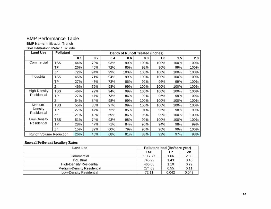
98
BMP Performance Table BMP Name: Infiltration Trench Soil Infiltration Rate: 1.02 in/hr
Depth of Runoff Treated (inches) Land Use Pollutant
0.1 0.2 0.4 0.6 0.8 1.0 1.5 2.0 TSS 44% 70% 93% 99% 100% 100% 100% 100% TP 26% 46% 72% 85% 92% 96% 99% 100%
Commercial
Zn 72% 94% 99% 100% 100% 100% 100% 100% TSS 45% 71% 94% 99% 100% 100% 100% 100% TP 27% 47% 73% 86% 92% 96% 99% 100%
Industrial
Zn 46% 76% 98% 99% 100% 100% 100% 100% TSS 46% 72% 94% 99% 100% 100% 100% 100% TP 27% 47% 73% 86% 92% 96% 99% 100%
High-Density Residential
Zn 54% 84% 98% 99% 100% 100% 100% 100% TSS 55% 80% 97% 99% 100% 100% 100% 100% TP 27% 47% 72% 85% 91% 95% 98% 99%
Medium-Density
Residential Zn 21% 40% 69% 86% 95% 99% 100% 100% TSS 51% 74% 93% 98% 99% 100% 100% 100% TP 28% 47% 71% 84% 90% 94% 98% 99%
Low-Density Residential
Zn 15% 32% 60% 79% 90% 96% 99% 100%
Runoff Volume Reduction 26% 45% 68% 81% 88% 92% 97% 98%
Annual Pollutant Loading Rates
Pollutant load (lbs/acre-year) Land use TSS TP Zn
Commercial 1117.77 1.66 2.33 Industrial 745.22 1.43 0.45
High-Density Residential 465.08 1.10 0.79 Medium-Density Residential 274.63 0.55 0.11
Low-Density Residential 72.11 0.042 0.043

BMP Performance Curve: Infiltration Trench
99
BMP Performance Curve: Infiltration TrenchLand Use: Commercial
(Soil infiltration rate 1.02 in/hr)
0%
10%
20%
30%
40%
50%
60%
70%
80%
90%
100%
0 0.2 0.4 0.6 0.8 1 1.2 1.4 1.6 1.8 2
Depth of Runoff Treated (inches)
Po
lluta
nt
Rem
ova
l
0%
10%
20%
30%
40%
50%
60%
70%
80%
90%
100%
Ru
no
ff V
olu
me
Red
uct
ion
TSS TP Zn Volume

100
BMP Performance Curve: Infiltration TrenchLand Use: Industrial
(Soil Infiltration Rate 1.02 in/hr)
0%
10%
20%
30%
40%
50%
60%
70%
80%
90%
100%
0 0.2 0.4 0.6 0.8 1 1.2 1.4 1.6 1.8 2
Depth of Runoff Treated (inches)
Po
lluta
nt R
emo
val
0%
10%
20%
30%
40%
50%
60%
70%
80%
90%
100%
Ru
no
ff V
olu
me
Red
uct
ion
TSS TP Zn Volume

BMP Performance Curve: Infiltration Trench
101
BMP Performance Curve: Infiltration TrenchLand Use: High Density Residential
(Soil infiltration rate 1.02 in/hr)
0%
10%
20%
30%
40%
50%
60%
70%
80%
90%
100%
0 0.2 0.4 0.6 0.8 1 1.2 1.4 1.6 1.8 2
Depth of Runoff Treated (inches)
Po
lltan
t R
emov
al
0%
10%
20%
30%
40%
50%
60%
70%
80%
90%
100%
Ru
nof
f V
olu
me
Red
uct
ion
TSS TP Zn Volume

102
BMP Performance Curve: Infiltration TrenchLand Use: Medium Density Residential
(Soil Infiltration Rate 1.02 in/hr)
0%
10%
20%
30%
40%
50%
60%
70%
80%
90%
100%
0 0.2 0.4 0.6 0.8 1 1.2 1.4 1.6 1.8 2
Depth of Runoff Treated
Po
lluta
nt
Rem
ova
l
0%
10%
20%
30%
40%
50%
60%
70%
80%
90%
100%
Ru
no
ff V
olu
me
Red
uct
ion
TSS TP Zn Volume

BMP Performance Curve: Infiltration Trench
103
BMP Performance Curve: Infiltration TrenchLand Use: Low Density Residential
(Soil Infiltration Rate 1.02 in/hr)
0%
10%
20%
30%
40%
50%
60%
70%
80%
90%
100%
0 0.2 0.4 0.6 0.8 1 1.2 1.4 1.6 1.8 2
Depth of Runoff Treated
Po
lluta
nt
Rem
ova
l
0%
10%
20%
30%
40%
50%
60%
70%
80%
90%
100%
Ru
no
ff V
olu
me
Red
uct
ion
TSS TP Zn Volume

104
BMP Performance Table BMP Name: Infiltration Trench Soil Infiltration Rate: 2.41 in/hr
Depth of Runoff Treated (inches) Land Use Pollutant
0.1 0.2 0.4 0.6 0.8 1 1.5 2 TSS 50% 77% 97% 100% 100% 100% 100% 100% TP 32% 55% 81% 91% 96% 98% 100% 100%
Commercial
Zn 81% 98% 100% 100% 100% 100% 100% 100% TSS 51% 78% 97% 100% 100% 100% 100% 100% TP 33% 56% 81% 92% 96% 98% 100% 100%
Industrial
Zn 55% 84% 99% 100% 100% 100% 100% 100% TSS 52% 79% 97% 100% 100% 100% 100% 100% TP 33% 55% 81% 91% 96% 98% 100% 100%
High-Density Residential
Zn 63% 92% 100% 100% 100% 100% 100% 100% TSS 62% 86% 98% 100% 100% 100% 100% 100% TP 33% 55% 80% 90% 95% 97% 99% 100%
Medium-Density
Residential Zn 25% 48% 79% 94% 99% 100% 100% 100% TSS 57% 80% 96% 99% 100% 100% 100% 100% TP 35% 56% 80% 90% 95% 97% 99% 100%
Low-Density Residential
Zn 19% 39% 71% 89% 97% 100% 100% 100%
Runoff Volume Reduction 34% 55% 78% 88% 93% 96% 99% 100%
Annual Pollutant Loading Rates
Pollutant load (lbs/acre-year) Land use TSS TP Zn
Commercial 1117.77 1.66 2.33 Industrial 745.22 1.43 0.45
High-Density Residential 465.08 1.10 0.79 Medium-Density Residential 274.63 0.55 0.11
Low-Density Residential 72.11 0.042 0.043
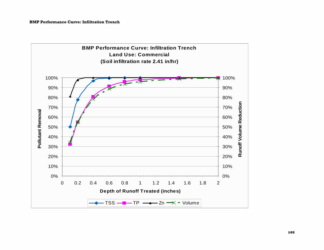
BMP Performance Curve: Infiltration Trench
105
BMP Performance Curve: Infiltration TrenchLand Use: Commercial
(Soil infiltration rate 2.41 in/hr)
0%
10%
20%
30%
40%
50%
60%
70%
80%
90%
100%
0 0.2 0.4 0.6 0.8 1 1.2 1.4 1.6 1.8 2
Depth of Runoff Treated (inches)
Po
lluta
nt
Rem
ova
l
0%
10%
20%
30%
40%
50%
60%
70%
80%
90%
100%
Ru
no
ff V
olu
me
Red
uct
ion
TSS TP Zn Volume
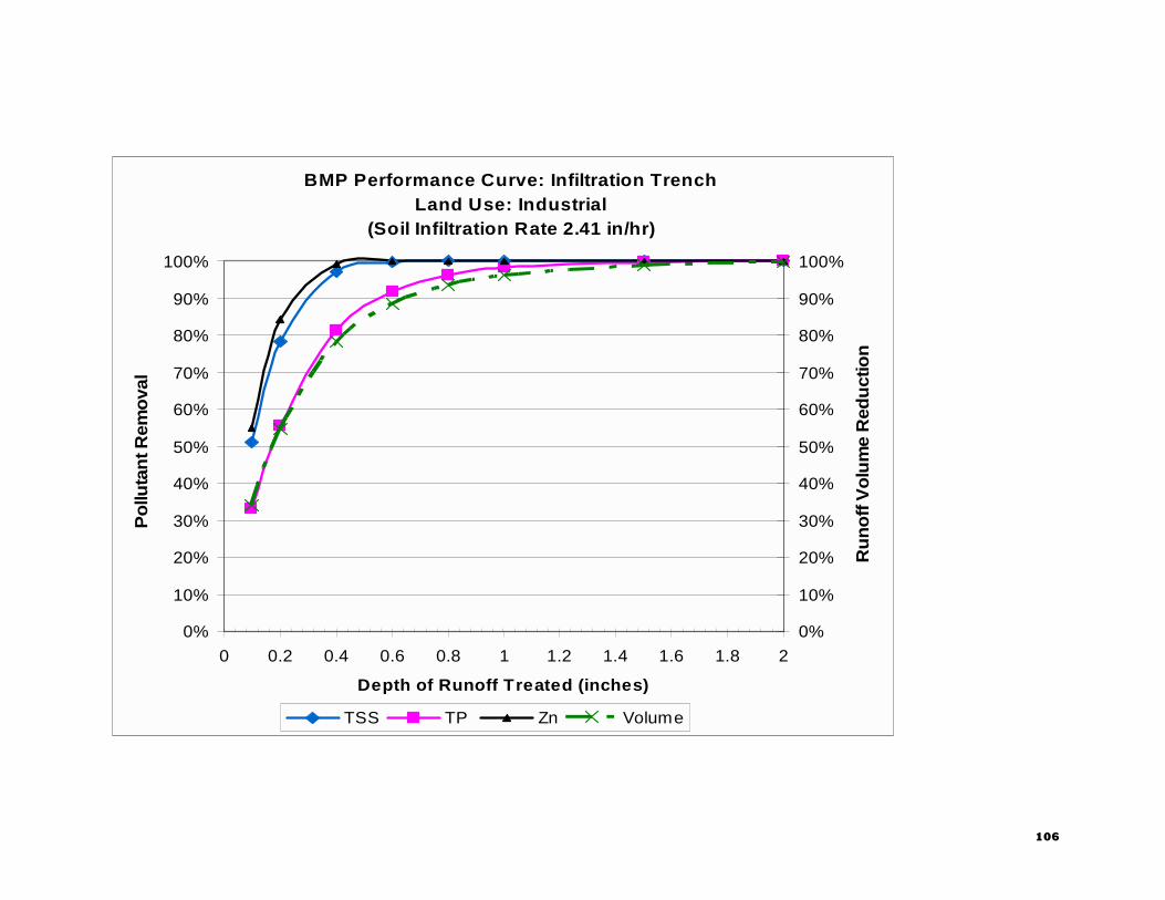
106
BMP Performance Curve: Infiltration TrenchLand Use: Industrial
(Soil Infiltration Rate 2.41 in/hr)
0%
10%
20%
30%
40%
50%
60%
70%
80%
90%
100%
0 0.2 0.4 0.6 0.8 1 1.2 1.4 1.6 1.8 2
Depth of Runoff Treated (inches)
Po
lluta
nt R
emo
val
0%
10%
20%
30%
40%
50%
60%
70%
80%
90%
100%
Ru
no
ff V
olu
me
Red
uct
ion
TSS TP Zn Volume

BMP Performance Curve: Infiltration Trench
107
BMP Performance Curve: Infiltration TrenchLand Use: High Density Residential
(Soil infiltration rate 2.41 in/hr)
0%
10%
20%
30%
40%
50%
60%
70%
80%
90%
100%
0 0.2 0.4 0.6 0.8 1 1.2 1.4 1.6 1.8 2
Depth of Runoff Treated (inches)
Po
lltan
t R
emo
val
0%
10%
20%
30%
40%
50%
60%
70%
80%
90%
100%
Ru
noff
Vo
lum
e R
edu
ctio
n
TSS TP Zn Volume

108
BMP Performance Curve: Infiltration TrenchLand Use: Medium Density Residential
(Soil Infiltration Rate 2.41 in/hr)
0%
10%
20%
30%
40%
50%
60%
70%
80%
90%
100%
0 0.2 0.4 0.6 0.8 1 1.2 1.4 1.6 1.8 2
Depth of Runoff Treated
Po
lluta
nt
Rem
ova
l
0%
10%
20%
30%
40%
50%
60%
70%
80%
90%
100%
Ru
noff
Vo
lum
e R
edu
ctio
n
TSS TP Zn Volume
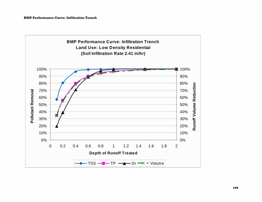
BMP Performance Curve: Infiltration Trench
109
BMP Performance Curve: Infiltration TrenchLand Use: Low Density Residential
(Soil Infiltration Rate 2.41 in/hr)
0%
10%
20%
30%
40%
50%
60%
70%
80%
90%
100%
0 0.2 0.4 0.6 0.8 1 1.2 1.4 1.6 1.8 2
Depth of Runoff Treated
Pol
luta
nt R
emo
val
0%
10%
20%
30%
40%
50%
60%
70%
80%
90%
100%
Ru
noff
Vo
lum
e R
edu
ctio
n
TSS TP Zn Volume

110
BMP Performance Table BMP Name: Infiltration Trench Soil Infiltration Rate: 8.27 in/hr
Depth of Runoff Treated (inches) Land Use Pollutant
0.1 0.2 0.4 0.6 0.8 1 1.5 2 TSS 68% 92% 100% 100% 100% 100% 100% 100% TP 50% 75% 94% 98% 99% 100% 100% 100%
Commercial
Zn 93% 100% 100% 100% 100% 100% 100% 100% TSS 69% 93% 100% 100% 100% 100% 100% 100% TP 51% 76% 94% 98% 100% 100% 100% 100%
Industrial
Zn 77% 99% 100% 100% 100% 100% 100% 100% TSS 70% 93% 100% 100% 100% 100% 100% 100% TP 50% 75% 94% 98% 99% 100% 100% 100%
High-Density Residential
Zn 84% 99% 100% 100% 100% 100% 100% 100% TSS 78% 95% 100% 100% 100% 100% 100% 100% TP 51% 75% 93% 98% 99% 100% 100% 100%
Medium-Density
Residential Zn 41% 70% 97% 100% 100% 100% 100% 100% TSS 73% 92% 99% 100% 100% 100% 100% 100% TP 53% 76% 93% 98% 99% 100% 100% 100%
Low-Density Residential
Zn 32% 60% 93% 100% 100% 100% 100% 100%
Runoff Volume Reduction 54% 76% 93% 97% 99% 100% 100% 100%
Annual Pollutant Loading Rates
Pollutant load (lbs/acre-year) Land use TSS TP Zn
Commercial 1117.77 1.66 2.33 Industrial 745.22 1.43 0.45
High-Density Residential 465.08 1.10 0.79 Medium-Density Residential 274.63 0.55 0.11
Low-Density Residential 72.11 0.042 0.043

BMP Performance Curve: Infiltration Trench
111
BMP Performance Curve: Infiltration TrenchLand Use: Commercial
(Soil infiltration rate 8.27 in/hr)
0%
10%
20%
30%
40%
50%
60%
70%
80%
90%
100%
0 0.2 0.4 0.6 0.8 1 1.2 1.4 1.6 1.8 2
Depth of Runoff Treated (inches)
Po
lluta
nt
Rem
ova
l
0%
10%
20%
30%
40%
50%
60%
70%
80%
90%
100%
Ru
no
ff V
olu
me
Red
uct
ion
TSS TP Zn Volume
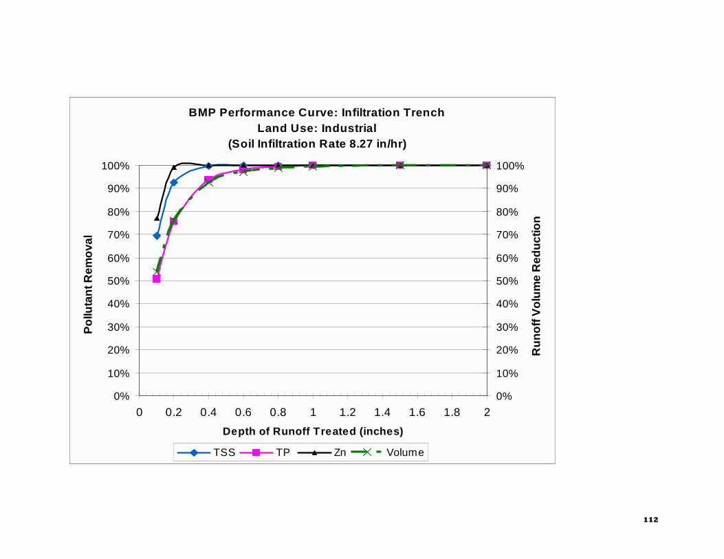
112
BMP Performance Curve: Infiltration TrenchLand Use: Industrial
(Soil Infiltration Rate 8.27 in/hr)
0%
10%
20%
30%
40%
50%
60%
70%
80%
90%
100%
0 0.2 0.4 0.6 0.8 1 1.2 1.4 1.6 1.8 2
Depth of Runoff Treated (inches)
Po
lluta
nt R
emo
val
0%
10%
20%
30%
40%
50%
60%
70%
80%
90%
100%
Ru
no
ff V
olu
me
Red
uct
ion
TSS TP Zn Volume

BMP Performance Curve: Infiltration Trench
113
BMP Performance Curve: Infiltration TrenchLand Use: High Density Residential
(Soil infiltration rate 8.27 in/hr)
0%
10%
20%
30%
40%
50%
60%
70%
80%
90%
100%
0 0.2 0.4 0.6 0.8 1 1.2 1.4 1.6 1.8 2
Depth of Runoff Treated (inches)
Po
lltan
t R
emo
val
0%
10%
20%
30%
40%
50%
60%
70%
80%
90%
100%
Ru
noff
Vo
lum
e R
edu
ctio
n
TSS TP Zn Volume

114
BMP Performance Curve: Infiltration TrenchLand Use: Medium Density Residential
(Soil Infiltration Rate 8.27 in/hr)
0%
10%
20%
30%
40%
50%
60%
70%
80%
90%
100%
0 0.2 0.4 0.6 0.8 1 1.2 1.4 1.6 1.8 2
Depth of Runoff Treated
Po
lluta
nt
Rem
ova
l
0%
10%
20%
30%
40%
50%
60%
70%
80%
90%
100%
Ru
no
ff V
olu
me
Red
uct
ion
TSS TP Zn Volume
BMP Performance Curve: Infiltration Trench
115
BMP Performance Curve: Infiltration
Basin
Prepared for: United States Environmental Protection Agency – Region 1 One Congress Street, Suite 1100 Boston, MA 02114 Prepared by: Tetra Tech, Inc. 10306 Eaton Place, Suite 340 Fairfax, VA 22030 September 2008

BMP Performance Table BMP Name: Infiltration Basin Soil Infiltration Rate: 0.17 in/hr
Depth of Runoff Treated (inches) Land Use Pollutant
0.1 0.2 0.4 0.6 0.8 1.0 1.5 2.0 TSS 45% 66% 87% 95% 98% 99% 100% 100% TP 27% 43% 65% 78% 86% 90% 96% 98%
Commercial
Zn 59% 79% 93% 97% 99% 99% 100% 100% TSS 46% 67% 87% 95% 98% 99% 100% 100% TP 27% 44% 65% 78% 86% 91% 97% 98%
Industrial
Zn 43% 64% 86% 94% 97% 99% 100% 100% TSS 46% 68% 88% 95% 98% 99% 100% 100% TP 27% 44% 65% 78% 86% 90% 96% 98%
High-Density Residential
Zn 48% 69% 89% 96% 98% 99% 100% 100% TSS 53% 74% 91% 97% 99% 100% 100% 100% TP 28% 44% 65% 78% 85% 90% 96% 98%
Medium-Density
Residential Zn 25% 42% 64% 78% 87% 92% 98% 99% TSS 51% 70% 88% 95% 98% 99% 100% 100% TP 29% 45% 65% 77% 85% 89% 95% 98%
Low-Density Residential
Zn 20% 35% 58% 73% 82% 89% 97% 99%
Runoff Volume Reduction 13% 24% 44% 59% 70% 78% 89% 94%
Annual Pollutant Loading Rates
Pollutant load (lbs/acre-year) Land use TSS TP Zn
Commercial 1117.77 1.66 2.33 Industrial 745.22 1.43 0.45
High-Density Residential 465.08 1.10 0.79 Medium-Density Residential 274.63 0.55 0.11
Low-Density Residential 72.11 0.042 0.043

BMP Performance Curve: Infiltration Basin
117
BMP Performance Curve: Infiltration BasinLand Use: Commercial
(Soil infiltration rate 0.17 in/hr)
0%
10%
20%
30%
40%
50%
60%
70%
80%
90%
100%
0 0.2 0.4 0.6 0.8 1 1.2 1.4 1.6 1.8 2
Depth of Runoff Treated (inches)
Po
lluta
nt
Rem
ova
l
0%
10%
20%
30%
40%
50%
60%
70%
80%
90%
100%
Ru
no
ff V
olu
me
Red
uct
ion
TSS TP Zn Volume

118
BMP Performance Curve: Infiltration BasinLand Use: Industrial
(Soil Infiltration Rate 0.17 in/hr)
0%
10%
20%
30%
40%
50%
60%
70%
80%
90%
100%
0 0.2 0.4 0.6 0.8 1 1.2 1.4 1.6 1.8 2
Depth of Runoff Treated (inches)
Po
lluta
nt R
emo
val
0%
10%
20%
30%
40%
50%
60%
70%
80%
90%
100%
Ru
no
ff V
olu
me
Red
uct
ion
TSS TP Zn Volume

BMP Performance Curve: Infiltration Basin
119
BMP Performance Curve: Infiltration BasinLand Use: High Density Residential
(Soil infiltration rate 0.17 in/hr)
0%
10%
20%
30%
40%
50%
60%
70%
80%
90%
100%
0 0.2 0.4 0.6 0.8 1 1.2 1.4 1.6 1.8 2
Depth of Runoff Treated (inches)
Po
lltan
t R
emo
val
0%
10%
20%
30%
40%
50%
60%
70%
80%
90%
100%
Ru
no
ff V
olu
me
Red
uct
ion
TSS TP Zn Volume

120
BMP Performance Curve: Infiltration BasinLand Use: Medium Density Residential
(Soil Infiltration Rate 0.17 in/hr)
0%
10%
20%
30%
40%
50%
60%
70%
80%
90%
100%
0 0.2 0.4 0.6 0.8 1 1.2 1.4 1.6 1.8 2
Depth of Runoff Treated
Po
lluta
nt R
emo
val
0%
10%
20%
30%
40%
50%
60%
70%
80%
90%
100%
Ru
noff
Vo
lum
e R
edu
ctio
n
TSS TP Zn Volume

BMP Performance Curve: Infiltration Basin
121
BMP Performance Curve: Infiltration BasinLand Use: Low Density Residential
(Soil Infiltration Rate 0.17 in/hr)
0%
10%
20%
30%
40%
50%
60%
70%
80%
90%
100%
0 0.2 0.4 0.6 0.8 1 1.2 1.4 1.6 1.8 2
Depth of Runoff Treated
Po
lluta
nt
Rem
ova
l
0%
10%
20%
30%
40%
50%
60%
70%
80%
90%
100%
Ru
no
ff V
olu
me
Red
uct
ion
TSS TP Zn Volume
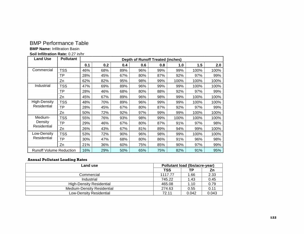
122
BMP Performance Table BMP Name: Infiltration Basin Soil Infiltration Rate: 0.27 in/hr
Depth of Runoff Treated (inches) Land Use Pollutant
0.1 0.2 0.4 0.6 0.8 1.0 1.5 2.0 TSS 46% 68% 89% 96% 99% 99% 100% 100% TP 28% 45% 67% 80% 87% 92% 97% 99%
Commercial
Zn 62% 82% 95% 98% 99% 100% 100% 100% TSS 47% 69% 89% 96% 99% 99% 100% 100% TP 28% 46% 68% 80% 88% 92% 97% 99%
Industrial
Zn 45% 67% 89% 96% 98% 99% 100% 100% TSS 48% 70% 89% 96% 99% 99% 100% 100% TP 28% 45% 67% 80% 87% 92% 97% 99%
High-Density Residential
Zn 50% 72% 92% 97% 99% 99% 100% 100% TSS 55% 76% 93% 98% 99% 100% 100% 100% TP 29% 46% 67% 80% 87% 91% 97% 98%
Medium-Density
Residential Zn 26% 43% 67% 81% 89% 94% 99% 100% TSS 53% 72% 90% 96% 98% 99% 100% 100% TP 30% 47% 68% 80% 86% 91% 96% 98%
Low-Density Residential
Zn 21% 36% 60% 75% 85% 90% 97% 99%
Runoff Volume Reduction 16% 29% 50% 65% 75% 82% 91% 95%
Annual Pollutant Loading Rates
Pollutant load (lbs/acre-year) Land use TSS TP Zn
Commercial 1117.77 1.66 2.33 Industrial 745.22 1.43 0.45
High-Density Residential 465.08 1.10 0.79 Medium-Density Residential 274.63 0.55 0.11
Low-Density Residential 72.11 0.042 0.043

BMP Performance Curve: Infiltration Basin
123
BMP Performance Curve: Infiltration BasinLand Use: Commercial
(Soil infiltration rate 0.27 in/hr)
0%
10%
20%
30%
40%
50%
60%
70%
80%
90%
100%
0 0.2 0.4 0.6 0.8 1 1.2 1.4 1.6 1.8 2
Depth of Runoff Treated (inches)
Po
lluta
nt
Rem
ova
l
0%
10%
20%
30%
40%
50%
60%
70%
80%
90%
100%
Ru
no
ff V
olu
me
Red
uct
ion
TSS TP Zn Volume
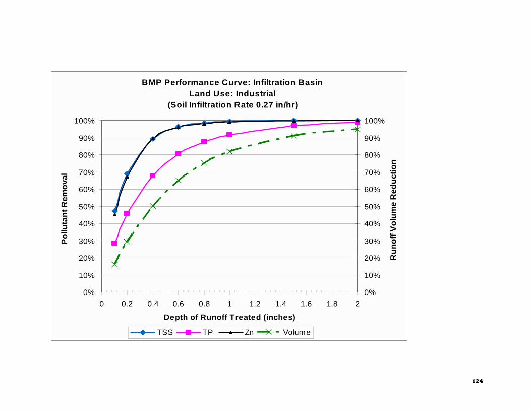
124
BMP Performance Curve: Infiltration BasinLand Use: Industrial
(Soil Infiltration Rate 0.27 in/hr)
0%
10%
20%
30%
40%
50%
60%
70%
80%
90%
100%
0 0.2 0.4 0.6 0.8 1 1.2 1.4 1.6 1.8 2
Depth of Runoff Treated (inches)
Po
lluta
nt R
emo
val
0%
10%
20%
30%
40%
50%
60%
70%
80%
90%
100%
Ru
no
ff V
olu
me
Red
uct
ion
TSS TP Zn Volume

BMP Performance Curve: Infiltration Basin
125
BMP Performance Curve: Infiltration BasinLand Use: High Density Residential
(Soil infiltration rate 0.27 in/hr)
0%
10%
20%
30%
40%
50%
60%
70%
80%
90%
100%
0 0.2 0.4 0.6 0.8 1 1.2 1.4 1.6 1.8 2
Depth of Runoff Treated (inches)
Po
lltan
t R
emov
al
0%
10%
20%
30%
40%
50%
60%
70%
80%
90%
100%
Run
off
Vo
lum
e R
edu
ctio
n
TSS TP Zn Volume

126
BMP Performance Curve: Infiltration BasinLand Use: Medium Density Residential
(Soil Infiltration Rate 0.27 in/hr)
0%
10%
20%
30%
40%
50%
60%
70%
80%
90%
100%
0 0.2 0.4 0.6 0.8 1 1.2 1.4 1.6 1.8 2
Depth of Runoff Treated
Po
lluta
nt
Rem
ova
l
0%
10%
20%
30%
40%
50%
60%
70%
80%
90%
100%
Ru
no
ff V
olu
me
Red
uct
ion
TSS TP Zn Volume

BMP Performance Curve: Infiltration Basin
127
BMP Performance Curve: Infiltration BasinLand Use: Low Density Residential
(Soil Infiltration Rate 0.27 in/hr)
0%
10%
20%
30%
40%
50%
60%
70%
80%
90%
100%
0 0.2 0.4 0.6 0.8 1 1.2 1.4 1.6 1.8 2
Depth of Runoff Treated
Pol
luta
nt R
emo
val
0%
10%
20%
30%
40%
50%
60%
70%
80%
90%
100%
Ru
no
ff V
olu
me
Red
ucti
on
TSS TP Zn Volume

128
BMP Performance Table BMP Name: Infiltration Basin Soil Infiltration Rate: 0.52 in/hr
Depth of Runoff Treated (inches) Land Use Pollutant
0.1 0.2 0.4 0.6 0.8 1.0 1.5 2.0 TSS 48% 70% 90% 97% 99% 100% 100% 100% TP 29% 47% 69% 82% 89% 93% 98% 99%
Commercial
Zn 64% 85% 97% 99% 100% 100% 100% 100% TSS 48% 71% 90% 97% 99% 100% 100% 100% TP 29% 47% 70% 83% 89% 93% 98% 99%
Industrial
Zn 47% 70% 92% 97% 99% 100% 100% 100% TSS 49% 71% 91% 97% 99% 100% 100% 100% TP 29% 47% 70% 82% 89% 93% 98% 99%
High-Density Residential
Zn 52% 75% 94% 98% 99% 100% 100% 100% TSS 56% 77% 94% 98% 99% 100% 100% 100% TP 30% 48% 70% 82% 89% 92% 97% 99%
Medium-Density
Residential Zn 27% 45% 69% 83% 91% 95% 99% 100% TSS 54% 74% 91% 97% 99% 99% 100% 100% TP 31% 49% 70% 82% 88% 92% 97% 98%
Low-Density Residential
Zn 21% 38% 62% 77% 87% 92% 99% 100%
Runoff Volume Reduction 20% 34% 57% 71% 80% 86% 94% 96%
Annual Pollutant Loading Rates
Pollutant load (lbs/acre-year) Land use TSS TP Zn
Commercial 1117.77 1.66 2.33 Industrial 745.22 1.43 0.45
High-Density Residential 465.08 1.10 0.79 Medium-Density Residential 274.63 0.55 0.11
Low-Density Residential 72.11 0.042 0.043

BMP Performance Curve: Infiltration Basin
129
BMP Performance Curve: Infiltration BasinLand Use: Commercial
(Soil infiltration rate 0.52 in/hr)
0%
10%
20%
30%
40%
50%
60%
70%
80%
90%
100%
0 0.2 0.4 0.6 0.8 1 1.2 1.4 1.6 1.8 2
Depth of Runoff Treated (inches)
Po
lluta
nt
Rem
ova
l
0%
10%
20%
30%
40%
50%
60%
70%
80%
90%
100%
Ru
no
ff V
olu
me
Red
uct
ion
TSS TP Zn Volume

130
BMP Performance Curve: Infiltration BasinLand Use: Industrial
(Soil Infiltration Rate 0.52 in/hr)
0%
10%
20%
30%
40%
50%
60%
70%
80%
90%
100%
0 0.2 0.4 0.6 0.8 1 1.2 1.4 1.6 1.8 2
Depth of Runoff Treated (inches)
Po
lluta
nt R
emo
val
0%
10%
20%
30%
40%
50%
60%
70%
80%
90%
100%
Ru
no
ff V
olu
me
Red
uct
ion
TSS TP Zn Volume

BMP Performance Curve: Infiltration Basin
131
BMP Performance Curve: Infiltration BasinLand Use: High Density Residential
(Soil infiltration rate 0.52 in/hr)
0%
10%
20%
30%
40%
50%
60%
70%
80%
90%
100%
0 0.2 0.4 0.6 0.8 1 1.2 1.4 1.6 1.8 2
Depth of Runoff Treated (inches)
Po
lltan
t R
emov
al
0%
10%
20%
30%
40%
50%
60%
70%
80%
90%
100%
Ru
noff
Vo
lum
e R
edu
ctio
n
TSS TP Zn Volume
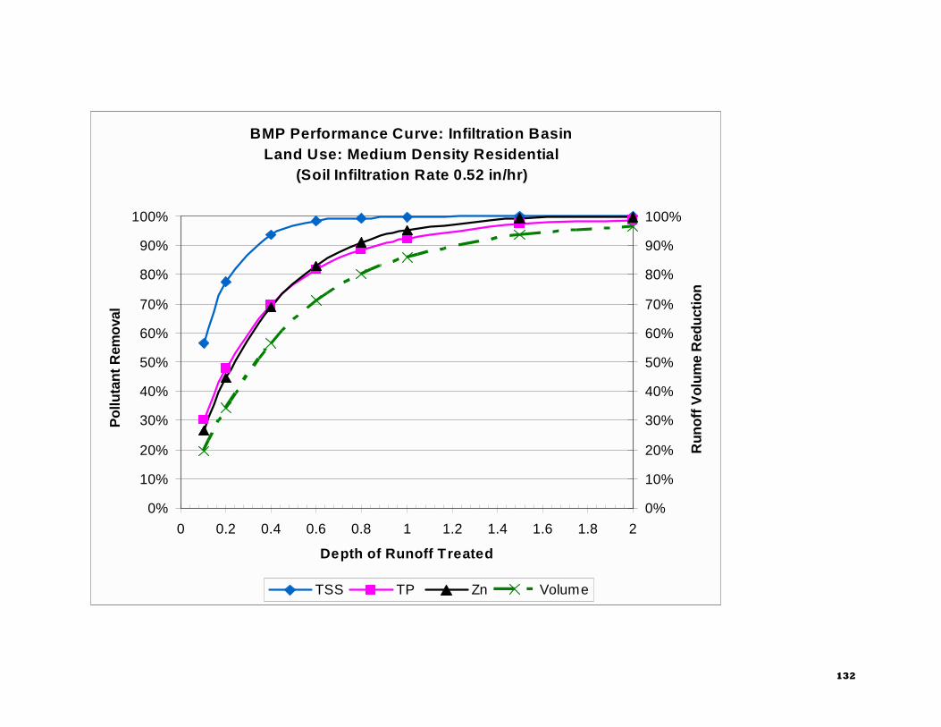
132
BMP Performance Curve: Infiltration BasinLand Use: Medium Density Residential
(Soil Infiltration Rate 0.52 in/hr)
0%
10%
20%
30%
40%
50%
60%
70%
80%
90%
100%
0 0.2 0.4 0.6 0.8 1 1.2 1.4 1.6 1.8 2
Depth of Runoff Treated
Po
lluta
nt
Rem
ova
l
0%
10%
20%
30%
40%
50%
60%
70%
80%
90%
100%
Run
off
Vol
um
e R
edu
ctio
n
TSS TP Zn Volume
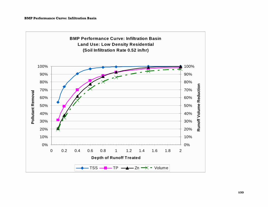
BMP Performance Curve: Infiltration Basin
133
BMP Performance Curve: Infiltration BasinLand Use: Low Density Residential
(Soil Infiltration Rate 0.52 in/hr)
0%
10%
20%
30%
40%
50%
60%
70%
80%
90%
100%
0 0.2 0.4 0.6 0.8 1 1.2 1.4 1.6 1.8 2
Depth of Runoff Treated
Po
lluta
nt R
emo
val
0%
10%
20%
30%
40%
50%
60%
70%
80%
90%
100%
Ru
noff
Vol
ume
Red
uct
ion
TSS TP Zn Volume

134
BMP Performance Table BMP Name: Infiltration Basin Soil Infiltration Rate: 1.02 in/hr
Depth of Runoff Treated (inches) Land Use Pollutant
0.1 0.2 0.4 0.6 0.8 1.0 1.5 2.0 TSS 49% 71% 92% 98% 99% 100% 100% 100% TP 30% 49% 72% 85% 91% 94% 98% 99%
Commercial
Zn 67% 88% 98% 99% 100% 100% 100% 100% TSS 49% 72% 92% 98% 99% 100% 100% 100% TP 31% 49% 73% 85% 91% 95% 98% 99%
Industrial
Zn 49% 73% 94% 98% 99% 100% 100% 100% TSS 50% 73% 92% 98% 99% 100% 100% 100% TP 30% 49% 72% 85% 91% 95% 98% 99%
High-Density Residential
Zn 54% 78% 96% 99% 100% 100% 100% 100% TSS 58% 79% 95% 99% 100% 100% 100% 100% TP 31% 50% 72% 84% 91% 94% 98% 99%
Medium-Density
Residential Zn 27% 46% 71% 86% 93% 97% 100% 100% TSS 55% 75% 92% 97% 99% 100% 100% 100% TP 33% 51% 73% 84% 90% 94% 98% 99%
Low-Density Residential
Zn 22% 39% 64% 80% 90% 95% 99% 100%
Runoff Volume Reduction 23% 39% 63% 77% 85% 90% 95% 98%
Annual Pollutant Loading Rates
Pollutant load (lbs/acre-year) Land use TSS TP Zn
Commercial 1117.77 1.66 2.33 Industrial 745.22 1.43 0.45
High-Density Residential 465.08 1.10 0.79 Medium-Density Residential 274.63 0.55 0.11
Low-Density Residential 72.11 0.042 0.043

BMP Performance Curve: Infiltration Basin
135
BMP Performance Curve: Infiltration BasinLand Use: Commercial
(Soil infiltration rate 1.02 in/hr)
0%
10%
20%
30%
40%
50%
60%
70%
80%
90%
100%
0 0.2 0.4 0.6 0.8 1 1.2 1.4 1.6 1.8 2
Depth of Runoff Treated (inches)
Po
lluta
nt
Rem
ova
l
0%
10%
20%
30%
40%
50%
60%
70%
80%
90%
100%
Ru
no
ff V
olu
me
Red
uct
ion
TSS TP Zn Volume
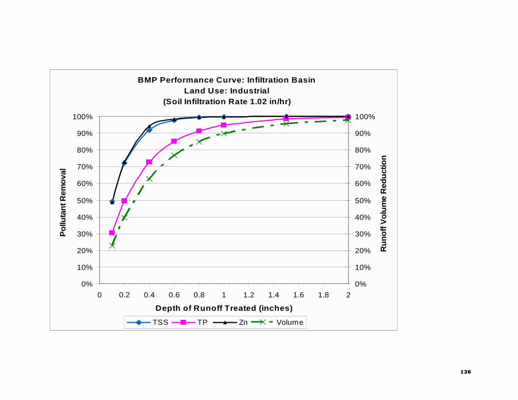
136
BMP Performance Curve: Infiltration BasinLand Use: Industrial
(Soil Infiltration Rate 1.02 in/hr)
0%
10%
20%
30%
40%
50%
60%
70%
80%
90%
100%
0 0.2 0.4 0.6 0.8 1 1.2 1.4 1.6 1.8 2
Depth of Runoff Treated (inches)
Po
lluta
nt R
emo
val
0%
10%
20%
30%
40%
50%
60%
70%
80%
90%
100%
Ru
no
ff V
olu
me
Red
uct
ion
TSS TP Zn Volume
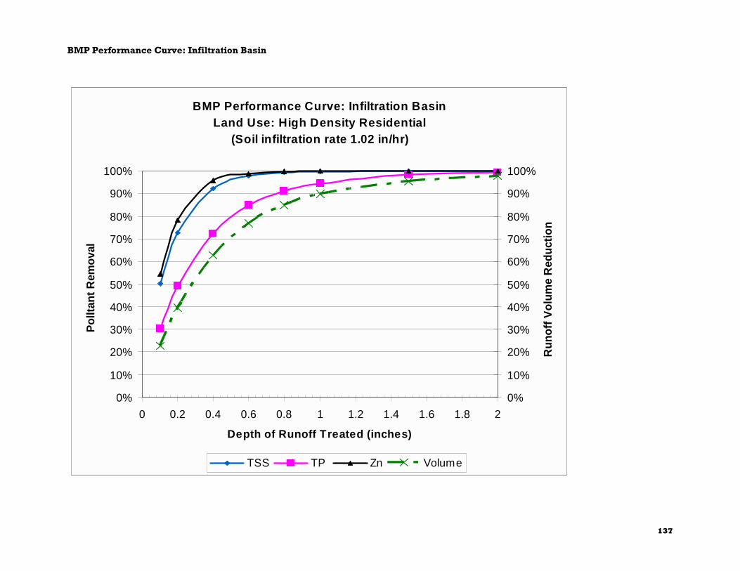
BMP Performance Curve: Infiltration Basin
137
BMP Performance Curve: Infiltration BasinLand Use: High Density Residential
(Soil infiltration rate 1.02 in/hr)
0%
10%
20%
30%
40%
50%
60%
70%
80%
90%
100%
0 0.2 0.4 0.6 0.8 1 1.2 1.4 1.6 1.8 2
Depth of Runoff Treated (inches)
Po
lltan
t R
emo
val
0%
10%
20%
30%
40%
50%
60%
70%
80%
90%
100%
Ru
no
ff V
olu
me
Red
uct
ion
TSS TP Zn Volume

138
BMP Performance Curve: Infiltration BasinLand Use: Medium Density Residential
(Soil Infiltration Rate 1.02 in/hr)
0%
10%
20%
30%
40%
50%
60%
70%
80%
90%
100%
0 0.2 0.4 0.6 0.8 1 1.2 1.4 1.6 1.8 2
Depth of Runoff Treated
Po
lluta
nt
Rem
ova
l
0%
10%
20%
30%
40%
50%
60%
70%
80%
90%
100%
Ru
no
ff V
olu
me
Red
uct
ion
TSS TP Zn Volume

BMP Performance Curve: Infiltration Basin
139
BMP Performance Curve: Infiltration BasinLand Use: Low Density Residential
(Soil Infiltration Rate 1.02 in/hr)
0%
10%
20%
30%
40%
50%
60%
70%
80%
90%
100%
0 0.2 0.4 0.6 0.8 1 1.2 1.4 1.6 1.8 2
Depth of Runoff Treated
Po
lluta
nt
Rem
ova
l
0%
10%
20%
30%
40%
50%
60%
70%
80%
90%
100%
Ru
no
ff V
olu
me
Red
uct
ion
TSS TP Zn Volume

140
BMP Performance Table BMP Name: Infiltration Basin Soil Infiltration Rate: 2.41 in/hr
Depth of Runoff Treated (inches) Land Use Pollutant
0.1 0.2 0.4 0.6 0.8 1 1.5 2 TSS 50% 74% 94% 99% 100% 100% 100% 100% TP 32% 52% 76% 88% 94% 97% 99% 100%
Commercial
Zn 71% 91% 99% 100% 100% 100% 100% 100% TSS 51% 75% 94% 99% 100% 100% 100% 100% TP 33% 53% 77% 89% 94% 97% 99% 100%
Industrial
Zn 51% 77% 97% 99% 100% 100% 100% 100% TSS 52% 75% 94% 99% 100% 100% 100% 100% TP 33% 53% 77% 88% 94% 97% 99% 100%
High-Density Residential
Zn 58% 83% 98% 100% 100% 100% 100% 100% TSS 59% 81% 96% 99% 100% 100% 100% 100% TP 34% 54% 77% 88% 93% 96% 99% 100%
Medium-Density
Residential Zn 28% 48% 75% 90% 97% 99% 100% 100% TSS 57% 78% 94% 98% 99% 100% 100% 100% TP 35% 55% 77% 88% 93% 96% 99% 100%
Low-Density Residential
Zn 22% 40% 68% 85% 94% 98% 100% 100%
Runoff Volume Reduction 28% 48% 72% 84% 90% 94% 98% 99%
Annual Pollutant Loading Rates
Pollutant load (lbs/acre-year) Land use TSS TP Zn
Commercial 1117.77 1.66 2.33 Industrial 745.22 1.43 0.45
High-Density Residential 465.08 1.10 0.79 Medium-Density Residential 274.63 0.55 0.11
Low-Density Residential 72.11 0.042 0.043

BMP Performance Curve: Infiltration Basin
141
BMP Performance Curve: Infiltration BasinLand Use: Commercial
(Soil infiltration rate 2.41 in/hr)
0%
10%
20%
30%
40%
50%
60%
70%
80%
90%
100%
0 0.2 0.4 0.6 0.8 1 1.2 1.4 1.6 1.8 2
Depth of Runoff Treated (inches)
Po
lluta
nt
Rem
ova
l
0%
10%
20%
30%
40%
50%
60%
70%
80%
90%
100%
Ru
no
ff V
olu
me
Red
uct
ion
TSS TP Zn Volume

142
BMP Performance Curve: Infiltration BasinLand Use: Industrial
(Soil Infiltration Rate 2.41 in/hr)
0%
10%
20%
30%
40%
50%
60%
70%
80%
90%
100%
0 0.2 0.4 0.6 0.8 1 1.2 1.4 1.6 1.8 2
Depth of Runoff Treated (inches)
Po
lluta
nt R
emo
val
0%
10%
20%
30%
40%
50%
60%
70%
80%
90%
100%
Ru
no
ff V
olu
me
Red
uct
ion
TSS TP Zn Volume

BMP Performance Curve: Infiltration Basin
143
BMP Performance Curve: Infiltration BasinLand Use: High Density Residential
(Soil infiltration rate 2.41 in/hr)
0%
10%
20%
30%
40%
50%
60%
70%
80%
90%
100%
0 0.2 0.4 0.6 0.8 1 1.2 1.4 1.6 1.8 2
Depth of Runoff Treated (inches)
Po
lltan
t R
emo
val
0%
10%
20%
30%
40%
50%
60%
70%
80%
90%
100%
Ru
no
ff V
olu
me
Red
uct
ion
TSS TP Zn Volume
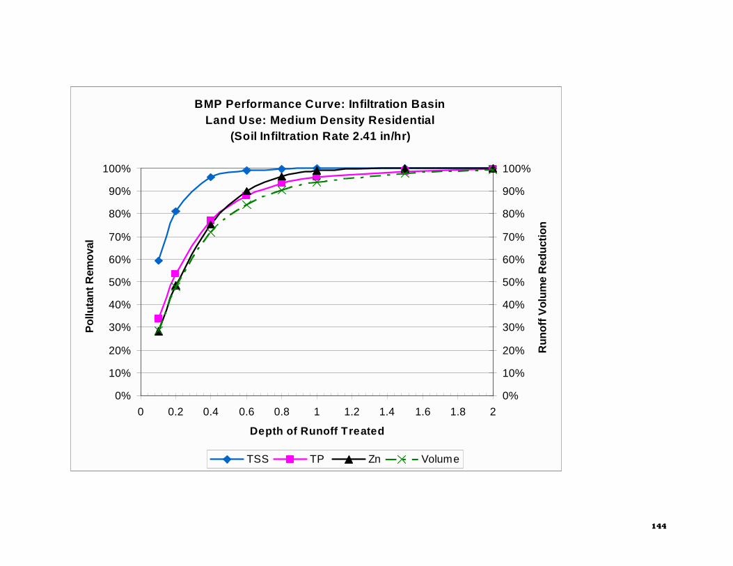
144
BMP Performance Curve: Infiltration BasinLand Use: Medium Density Residential
(Soil Infiltration Rate 2.41 in/hr)
0%
10%
20%
30%
40%
50%
60%
70%
80%
90%
100%
0 0.2 0.4 0.6 0.8 1 1.2 1.4 1.6 1.8 2
Depth of Runoff Treated
Po
lluta
nt
Rem
ova
l
0%
10%
20%
30%
40%
50%
60%
70%
80%
90%
100%
Run
off
Vol
um
e R
edu
ctio
n
TSS TP Zn Volume

BMP Performance Curve: Infiltration Basin
145
BMP Performance Curve: Infiltration BasinLand Use: Low Density Residential
(Soil Infiltration Rate 2.41 in/hr)
0%
10%
20%
30%
40%
50%
60%
70%
80%
90%
100%
0 0.2 0.4 0.6 0.8 1 1.2 1.4 1.6 1.8 2
Depth of Runoff Treated
Po
lluta
nt R
emo
val
0%
10%
20%
30%
40%
50%
60%
70%
80%
90%
100%
Run
off
Vo
lum
e R
educ
tion
TSS TP Zn Volume

146
BMP Performance Table BMP Name: Infiltration Basin Soil Infiltration Rate: 8.27 in/hr
Depth of Runoff Treated (inches) Land Use Pollutant
0.1 0.2 0.4 0.6 0.8 1 1.5 2 TSS 53% 78% 96% 99% 100% 100% 100% 100% TP 37% 59% 83% 93% 97% 98% 100% 100%
Commercial
Zn 76% 94% 99% 100% 100% 100% 100% 100% TSS 53% 79% 96% 99% 100% 100% 100% 100% TP 38% 60% 83% 93% 97% 98% 100% 100%
Industrial
Zn 57% 84% 99% 100% 100% 100% 100% 100% TSS 54% 79% 96% 99% 100% 100% 100% 100% TP 37% 60% 83% 92% 97% 98% 100% 100%
High-Density Residential
Zn 64% 89% 99% 100% 100% 100% 100% 100% TSS 62% 85% 97% 100% 100% 100% 100% 100% TP 38% 60% 83% 92% 96% 98% 100% 100%
Medium-Density
Residential Zn 31% 53% 81% 95% 99% 100% 100% 100% TSS 60% 81% 95% 99% 100% 100% 100% 100% TP 40% 62% 83% 92% 96% 98% 100% 100%
Low-Density Residential
Zn 24% 44% 73% 90% 98% 100% 100% 100%
Runoff Volume Reduction 38% 60% 82% 91% 96% 97% 99% 100%
Annual Pollutant Loading Rates
Pollutant load (lbs/acre-year) Land use TSS TP Zn
Commercial 1117.77 1.66 2.33 Industrial 745.22 1.43 0.45
High-Density Residential 465.08 1.10 0.79 Medium-Density Residential 274.63 0.55 0.11
Low-Density Residential 72.11 0.042 0.043
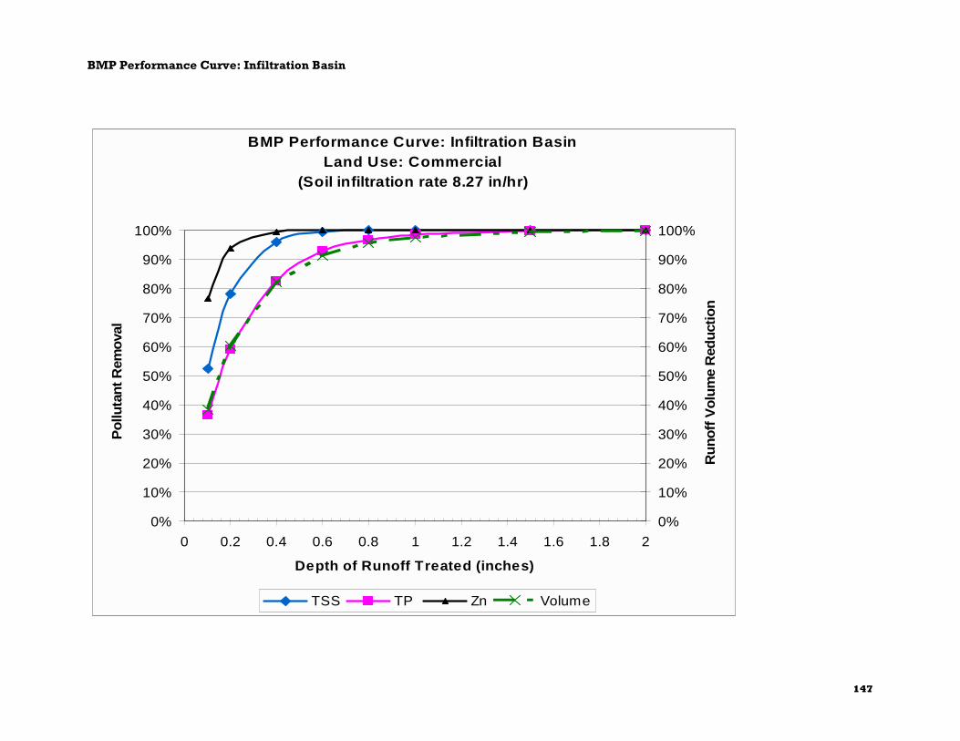
BMP Performance Curve: Infiltration Basin
147
BMP Performance Curve: Infiltration BasinLand Use: Commercial
(Soil infiltration rate 8.27 in/hr)
0%
10%
20%
30%
40%
50%
60%
70%
80%
90%
100%
0 0.2 0.4 0.6 0.8 1 1.2 1.4 1.6 1.8 2
Depth of Runoff Treated (inches)
Po
lluta
nt
Rem
ova
l
0%
10%
20%
30%
40%
50%
60%
70%
80%
90%
100%
Ru
no
ff V
olu
me
Red
uct
ion
TSS TP Zn Volume

148
BMP Performance Curve: Infiltration BasinLand Use: Industrial
(Soil Infiltration Rate 8.27 in/hr)
0%
10%
20%
30%
40%
50%
60%
70%
80%
90%
100%
0 0.2 0.4 0.6 0.8 1 1.2 1.4 1.6 1.8 2
Depth of Runoff Treated (inches)
Po
lluta
nt R
emo
val
0%
10%
20%
30%
40%
50%
60%
70%
80%
90%
100%
Ru
no
ff V
olu
me
Red
uct
ion
TSS TP Zn Volume
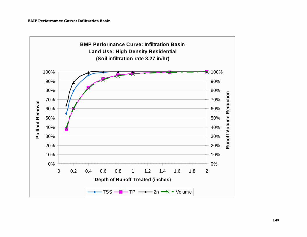
BMP Performance Curve: Infiltration Basin
149
BMP Performance Curve: Infiltration BasinLand Use: High Density Residential
(Soil infiltration rate 8.27 in/hr)
0%
10%
20%
30%
40%
50%
60%
70%
80%
90%
100%
0 0.2 0.4 0.6 0.8 1 1.2 1.4 1.6 1.8 2
Depth of Runoff Treated (inches)
Po
lltan
t R
emo
val
0%
10%
20%
30%
40%
50%
60%
70%
80%
90%
100%
Ru
no
ff V
olu
me
Red
uct
ion
TSS TP Zn Volume

150
BMP Performance Curve: Infiltration BasinLand Use: Medium Density Residential
(Soil Infiltration Rate 8.27 in/hr)
0%
10%
20%
30%
40%
50%
60%
70%
80%
90%
100%
0 0.2 0.4 0.6 0.8 1 1.2 1.4 1.6 1.8 2
Depth of Runoff Treated
Po
lluta
nt R
emov
al
0%
10%
20%
30%
40%
50%
60%
70%
80%
90%
100%
Run
off V
olu
me
Red
ucti
on
TSS TP Zn Volume

BMP Performance Curve: Infiltration Basin
151
BMP Performance Curve: Infiltration BasinLand Use: Low Density Residential
(Soil Infiltration Rate 8.27 in/hr)
0%
10%
20%
30%
40%
50%
60%
70%
80%
90%
100%
0 0.2 0.4 0.6 0.8 1 1.2 1.4 1.6 1.8 2
Depth of Runoff Treated
Pol
luta
nt R
emov
al
0%
10%
20%
30%
40%
50%
60%
70%
80%
90%
100%
Ru
noff
Vol
ume
Red
uct
ion
TSS TP Zn Volume

BMP Performance Curve: Gravel Wetland
Prepared for: United States Environmental Protection Agency – Region 1 One Congress Street, Suite 1100 Boston, MA 02114 Prepared by: Tetra Tech, Inc. 10306 Eaton Place, Suite 340 Fairfax, VA 22030 September 2008

BMP Performance Curve: Gravel Wetland
153
BMP Performance Table BMP Name: Gravel Wetland
Depth of Runoff Treated (inches) Land Use Pollutant
0.1 0.2 0.4 0.6 0.8 1.0 1.5 2.0 TSS 48% 61% 82% 91% 95% 97% 99% 99% TP 19% 26% 41% 51% 57% 61% 65% 66%
Commercial
Zn 57% 68% 83% 88% 90% 90% 91% 92% TSS 47% 61% 82% 91% 96% 97% 99% 99% TP 19% 27% 42% 51% 58% 61% 65% 66%
Industrial
Zn 40% 54% 74% 84% 88% 90% 90% 91% TSS 47% 62% 82% 92% 96% 98% 99% 99% TP 19% 26% 41% 51% 57% 61% 65% 66%
High-Density Residential
Zn 46% 59% 78% 86% 89% 90% 91% 91% TSS 53% 68% 86% 94% 97% 98% 99% 99% TP 20% 27% 42% 51% 57% 61% 65% 66%
Medium-Density
Residential Zn 21% 32% 52% 67% 76% 82% 89% 91% TSS 51% 65% 83% 92% 96% 97% 99% 99% TP 21% 28% 42% 51% 57% 61% 64% 66%
Low-Density Residential
Zn 16% 26% 46% 61% 71% 78% 87% 90%
Annual Pollutant Loading Rates
Pollutant load (lbs/acre-year) Land use TSS TP Zn
Commercial 1117.77 1.66 2.33 Industrial 745.22 1.43 0.45
High-Density Residential 465.08 1.10 0.79 Medium-Density Residential 274.63 0.55 0.11
Low-Density Residential 72.11 0.042 0.043
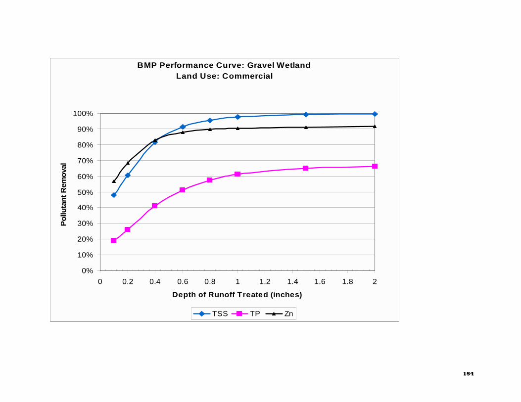
154
BMP Performance Curve: Gravel WetlandLand Use: Commercial
0%
10%
20%
30%
40%
50%
60%
70%
80%
90%
100%
0 0.2 0.4 0.6 0.8 1 1.2 1.4 1.6 1.8 2
Depth of Runoff Treated (inches)
Po
lluta
nt
Rem
ova
l
TSS TP Zn
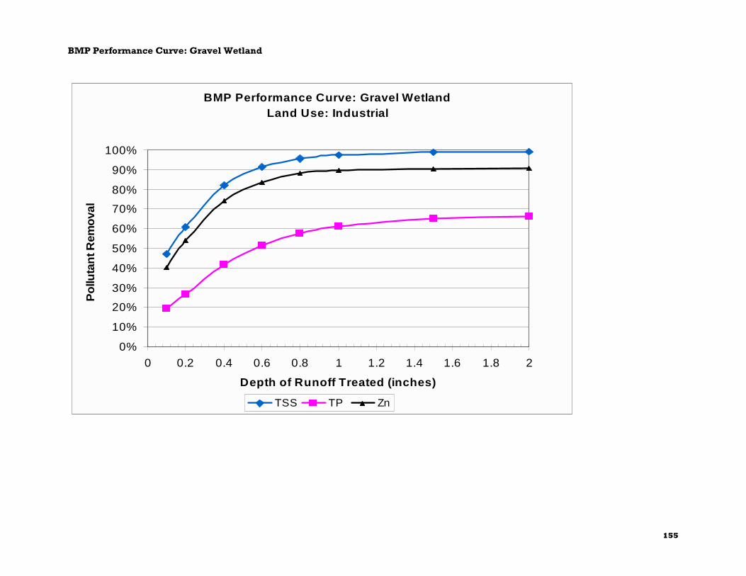
BMP Performance Curve: Gravel Wetland
155
BMP Performance Curve: Gravel WetlandLand Use: Industrial
0%
10%
20%
30%
40%
50%
60%
70%
80%
90%
100%
0 0.2 0.4 0.6 0.8 1 1.2 1.4 1.6 1.8 2
Depth of Runoff Treated (inches)
Po
lluta
nt R
emo
val
TSS TP Zn

156
BMP Performance Curve: Gravel WetlandLand Use: High Density Residential
0%
10%
20%
30%
40%
50%
60%
70%
80%
90%
100%
0 0.2 0.4 0.6 0.8 1 1.2 1.4 1.6 1.8 2
Depth of Runoff Treated (inches)
Po
lltan
t R
emo
val
TSS TP Zn

BMP Performance Curve: Gravel Wetland
157
BMP Performance Curve: Gravel WetlandLand Use: Medium Density Residential
0%
10%
20%
30%
40%
50%
60%
70%
80%
90%
100%
0 0.2 0.4 0.6 0.8 1 1.2 1.4 1.6 1.8 2
Depth of Runoff Treated
Po
lluta
nt
Rem
ova
l
TSS TP Zn

158
BMP Performance Curve: Gravel WetlandLand Use: Low Density Residential
0%
10%
20%
30%
40%
50%
60%
70%
80%
90%
100%
0 0.2 0.4 0.6 0.8 1 1.2 1.4 1.6 1.8 2
Depth of Runoff Treated
Po
lluta
nt
Rem
ova
l
TSS TP Zn

BMP Performance Curve: Bioretention
159
BMP Performance Curve: Bioretention
Prepared for: United States Environmental Protection Agency – Region 1 One Congress Street, Suite 1100 Boston, MA 02114 Prepared by: Tetra Tech, Inc. 10306 Eaton Place, Suite 340 Fairfax, VA 22030 September 2008

160
BMP Performance Table BMP Name: Bioretention
Depth of Runoff Treated (inches) Land Use Pollutant
0.1 0.2 0.4 0.6 0.8 1.0 1.5 2.0 TSS 44% 69% 91% 97% 98% 99% 100% 100% TP 19% 33% 53% 64% 71% 76% 84% 89%
Commercial
Zn 68% 88% 95% 96% 96% 97% 98% 99% TSS 45% 70% 91% 97% 98% 99% 100% 100% TP 20% 34% 53% 64% 71% 76% 84% 89%
Industrial
Zn 46% 72% 94% 96% 96% 96% 98% 99% TSS 46% 70% 92% 97% 99% 99% 100% 100% TP 19% 34% 53% 64% 71% 76% 84% 89%
High-Density Residential
Zn 53% 79% 95% 96% 96% 97% 98% 99% TSS 54% 78% 94% 98% 99% 99% 100% 100% TP 20% 34% 53% 63% 70% 75% 83% 88%
Medium-Density
Residential Zn 23% 41% 68% 83% 92% 95% 97% 97% TSS 52% 73% 91% 96% 98% 99% 99% 100% TP 21% 35% 52% 62% 68% 73% 81% 86%
Low-Density Residential
Zn 17% 33% 59% 76% 88% 93% 97% 97%
Annual Pollutant Loading Rates
Pollutant load (lbs/acre-year) Land use TSS TP Zn
Commercial 1117.77 1.66 2.33 Industrial 745.22 1.43 0.45
High-Density Residential 465.08 1.10 0.79 Medium-Density Residential 274.63 0.55 0.11
Low-Density Residential 72.11 0.042 0.043

BMP Performance Curve: Bioretention
161
BMP Performance Curve: BiorententionLand Use: Commercial
0%
10%
20%
30%
40%
50%
60%
70%
80%
90%
100%
0 0.2 0.4 0.6 0.8 1 1.2 1.4 1.6 1.8 2
Depth of Runoff Treated (inches)
Pollu
tant R
emova
l
TSS TP Zn

162
BMP Performance Curve: BioretentionLand Use: Industrial
0%
10%
20%
30%
40%
50%
60%
70%
80%
90%
100%
0 0.2 0.4 0.6 0.8 1 1.2 1.4 1.6 1.8 2
Depth of Runoff Treated (inches)
Pollu
tan
t Rem
ova
l
TSS TP Zn

BMP Performance Curve: Bioretention
163
BMP Performance Curve: BioretentionLand Use: High Density Residential
0%
10%
20%
30%
40%
50%
60%
70%
80%
90%
100%
0 0.2 0.4 0.6 0.8 1 1.2 1.4 1.6 1.8 2
Depth of Runoff Treated (inches)
Pollt
ant R
emova
l
TSS TP Zn

164
BMP Performance Curve: BioretentionLand Use: Medium Density Residential
0%
10%
20%
30%
40%
50%
60%
70%
80%
90%
100%
0 0.2 0.4 0.6 0.8 1 1.2 1.4 1.6 1.8 2
Depth of Runoff Treated
Pollu
tant R
emova
l
TSS TP Zn

BMP Performance Curve: Bioretention
165
BMP Performance Curve: BioretentionLand Use: Low Density Residential
0%
10%
20%
30%
40%
50%
60%
70%
80%
90%
100%
0 0.2 0.4 0.6 0.8 1 1.2 1.4 1.6 1.8 2
Depth of Runoff Treated
Pollu
tant R
emova
l
TSS TP Zn

166
BMP Performance Curve: Grass Swale
Prepared for: United States Environmental Protection Agency – Region 1 One Congress Street, Suite 1100 Boston, MA 02114 Prepared by: Tetra Tech, Inc. 10306 Eaton Place, Suite 340 Fairfax, VA 22030 September 2008
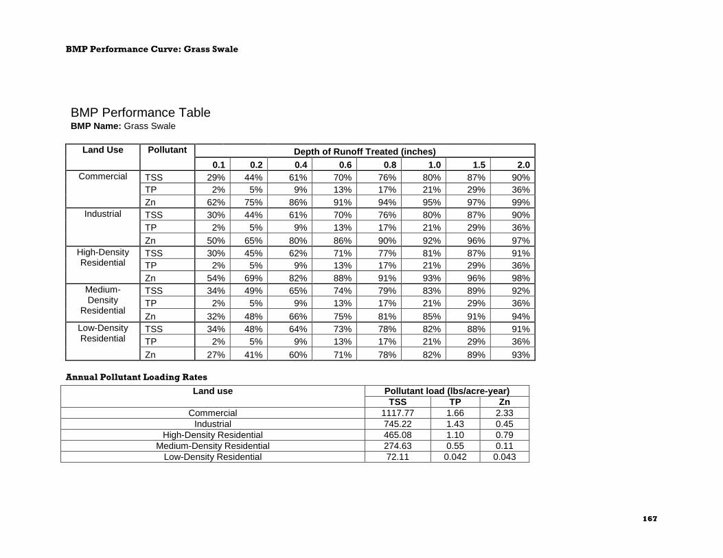
BMP Performance Curve: Grass Swale
167
BMP Performance Table BMP Name: Grass Swale
Depth of Runoff Treated (inches) Land Use Pollutant
0.1 0.2 0.4 0.6 0.8 1.0 1.5 2.0 TSS 29% 44% 61% 70% 76% 80% 87% 90% TP 2% 5% 9% 13% 17% 21% 29% 36%
Commercial
Zn 62% 75% 86% 91% 94% 95% 97% 99% TSS 30% 44% 61% 70% 76% 80% 87% 90% TP 2% 5% 9% 13% 17% 21% 29% 36%
Industrial
Zn 50% 65% 80% 86% 90% 92% 96% 97% TSS 30% 45% 62% 71% 77% 81% 87% 91% TP 2% 5% 9% 13% 17% 21% 29% 36%
High-Density Residential
Zn 54% 69% 82% 88% 91% 93% 96% 98% TSS 34% 49% 65% 74% 79% 83% 89% 92% TP 2% 5% 9% 13% 17% 21% 29% 36%
Medium-Density
Residential Zn 32% 48% 66% 75% 81% 85% 91% 94% TSS 34% 48% 64% 73% 78% 82% 88% 91% TP 2% 5% 9% 13% 17% 21% 29% 36%
Low-Density Residential
Zn 27% 41% 60% 71% 78% 82% 89% 93%
Annual Pollutant Loading Rates
Pollutant load (lbs/acre-year) Land use TSS TP Zn
Commercial 1117.77 1.66 2.33 Industrial 745.22 1.43 0.45
High-Density Residential 465.08 1.10 0.79 Medium-Density Residential 274.63 0.55 0.11
Low-Density Residential 72.11 0.042 0.043
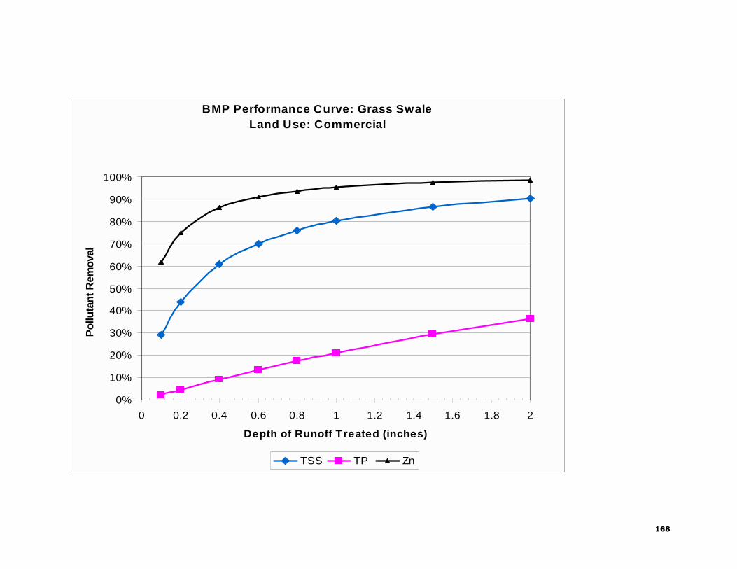
168
BMP Performance Curve: Grass SwaleLand Use: Commercial
0%
10%
20%
30%
40%
50%
60%
70%
80%
90%
100%
0 0.2 0.4 0.6 0.8 1 1.2 1.4 1.6 1.8 2
Depth of Runoff Treated (inches)
Po
lluta
nt
Rem
ova
l
TSS TP Zn

BMP Performance Curve: Grass Swale
169
BMP Performance Curve: Grass SwaleLand Use: Industrial
0%
10%
20%
30%
40%
50%
60%
70%
80%
90%
100%
0 0.2 0.4 0.6 0.8 1 1.2 1.4 1.6 1.8 2
Depth of Runoff Treated (inches)
Po
lluta
nt R
emo
val
TSS TP Zn

170
BMP Performance Curve: Grass SwaleLand Use: High Density Residential
0%
10%
20%
30%
40%
50%
60%
70%
80%
90%
100%
0 0.2 0.4 0.6 0.8 1 1.2 1.4 1.6 1.8 2
Depth of Runoff Treated (inches)
Po
lltan
t R
emo
val
TSS TP Zn

BMP Performance Curve: Grass Swale
171
BMP Performance Curve: Grass SwaleLand Use: Medium Density Residential
0%
10%
20%
30%
40%
50%
60%
70%
80%
90%
100%
0 0.2 0.4 0.6 0.8 1 1.2 1.4 1.6 1.8 2
Depth of Runoff Treated
Po
lluta
nt
Rem
ova
l
TSS TP Zn

172
BMP Performance Curve: Grass SwaleLand Use: Low Density Residential
0%
10%
20%
30%
40%
50%
60%
70%
80%
90%
100%
0 0.2 0.4 0.6 0.8 1 1.2 1.4 1.6 1.8 2
Depth of Runoff Treated
Po
lluta
nt
Rem
ova
l
TSS TP Zn

BMP Performance Curve: Wet Pond
173
BMP Performance Curve: Wet Pond
Prepared for: United States Environmental Protection Agency – Region 1 One Congress Street, Suite 1100 Boston, MA 02114 Prepared by Tetra Tech, Inc. 10306 Eaton Place, Suite 340 Fairfax, VA 22030 September 2008
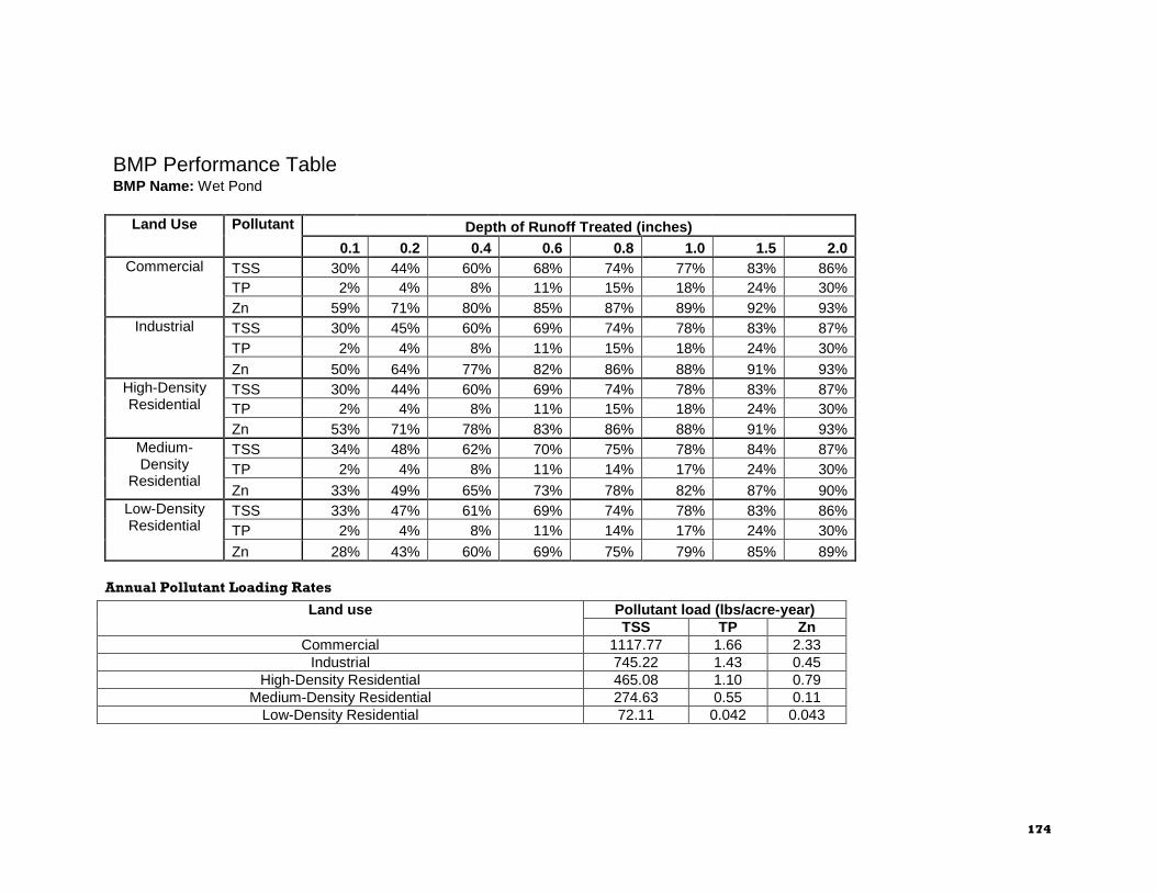
174
BMP Performance Table BMP Name: Wet Pond
Depth of Runoff Treated (inches) Land Use Pollutant
0.1 0.2 0.4 0.6 0.8 1.0 1.5 2.0 TSS 30% 44% 60% 68% 74% 77% 83% 86% TP 2% 4% 8% 11% 15% 18% 24% 30%
Commercial
Zn 59% 71% 80% 85% 87% 89% 92% 93% TSS 30% 45% 60% 69% 74% 78% 83% 87% TP 2% 4% 8% 11% 15% 18% 24% 30%
Industrial
Zn 50% 64% 77% 82% 86% 88% 91% 93% TSS 30% 44% 60% 69% 74% 78% 83% 87% TP 2% 4% 8% 11% 15% 18% 24% 30%
High-Density Residential
Zn 53% 71% 78% 83% 86% 88% 91% 93% TSS 34% 48% 62% 70% 75% 78% 84% 87% TP 2% 4% 8% 11% 14% 17% 24% 30%
Medium-Density
Residential Zn 33% 49% 65% 73% 78% 82% 87% 90% TSS 33% 47% 61% 69% 74% 78% 83% 86% TP 2% 4% 8% 11% 14% 17% 24% 30%
Low-Density Residential
Zn 28% 43% 60% 69% 75% 79% 85% 89%
Annual Pollutant Loading Rates
Pollutant load (lbs/acre-year) Land use TSS TP Zn
Commercial 1117.77 1.66 2.33 Industrial 745.22 1.43 0.45
High-Density Residential 465.08 1.10 0.79 Medium-Density Residential 274.63 0.55 0.11
Low-Density Residential 72.11 0.042 0.043
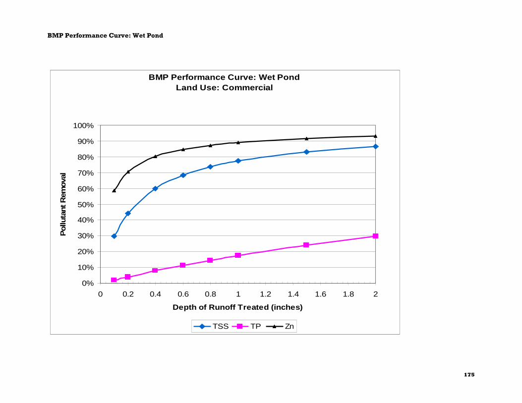
BMP Performance Curve: Wet Pond
175
BMP Performance Curve: Wet PondLand Use: Commercial
0%
10%
20%
30%
40%
50%
60%
70%
80%
90%
100%
0 0.2 0.4 0.6 0.8 1 1.2 1.4 1.6 1.8 2
Depth of Runoff Treated (inches)
Pollu
tant R
emova
l
TSS TP Zn

176
BMP Performance Curve: Wet PondLand Use: Industrial
0%
10%
20%
30%
40%
50%
60%
70%
80%
90%
100%
0 0.2 0.4 0.6 0.8 1 1.2 1.4 1.6 1.8 2
Depth of Runoff Treated (inches)
Pollu
tan
t Rem
ova
l
TSS TP Zn
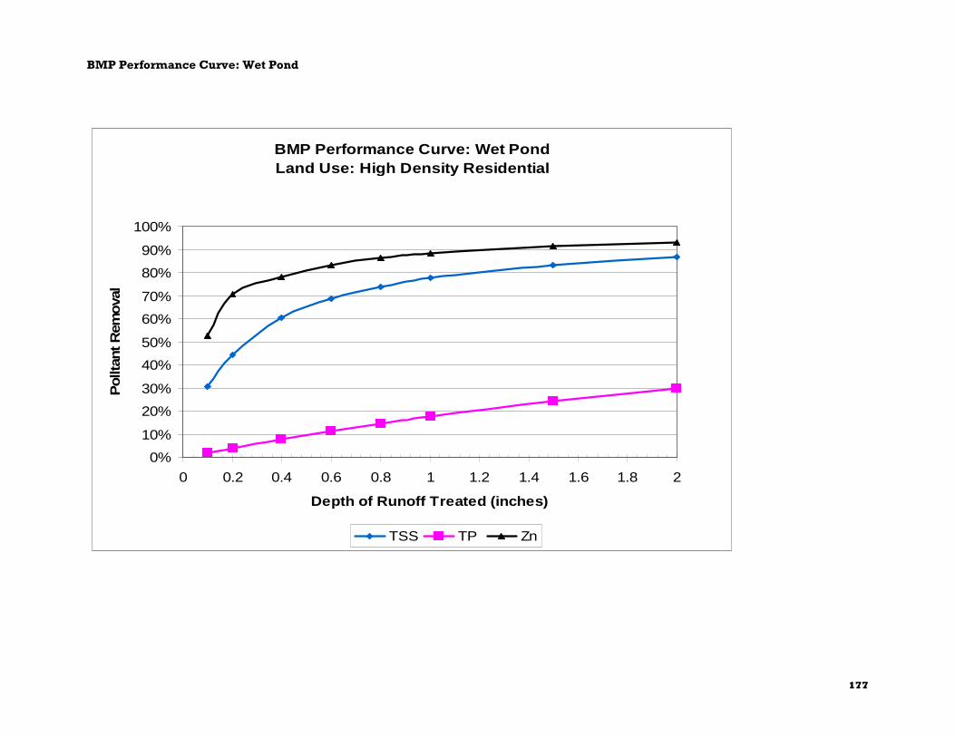
BMP Performance Curve: Wet Pond
177
BMP Performance Curve: Wet PondLand Use: High Density Residential
0%
10%
20%
30%
40%
50%
60%
70%
80%
90%
100%
0 0.2 0.4 0.6 0.8 1 1.2 1.4 1.6 1.8 2
Depth of Runoff Treated (inches)
Pollt
ant R
emova
l
TSS TP Zn

178
BMP Performance Curve: Wet PondLand Use: Medium Density Residential
0%
10%
20%
30%
40%
50%
60%
70%
80%
90%
100%
0 0.2 0.4 0.6 0.8 1 1.2 1.4 1.6 1.8 2
Depth of Runoff Treated
Pollu
tant R
emova
l
TSS TP Zn

BMP Performance Curve: Wet Pond
179
BMP Performance Curve: Wet PondLand Use: Low Density Residential
0%
10%
20%
30%
40%
50%
60%
70%
80%
90%
100%
0 0.2 0.4 0.6 0.8 1 1.2 1.4 1.6 1.8 2
Depth of Runoff Treated
Pollu
tant R
emova
l
TSS TP Zn

180
BMP Performance Curve: Dry Pond
Prepared for: United States Environmental Protection Agency – Region 1 One Congress Street, Suite 1100 Boston, MA 02114 Prepared by: Tetra Tech, Inc. 10306 Eaton Place, Suite 340 Fairfax, VA 22030 September 2008
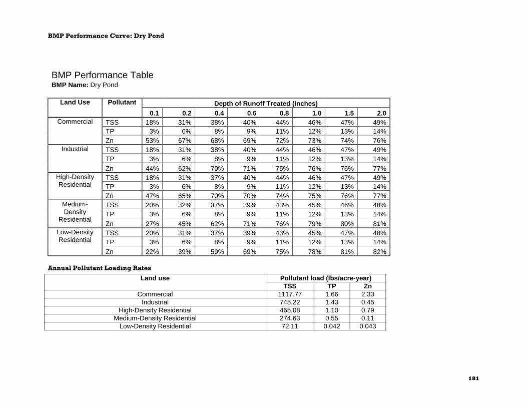
BMP Performance Curve: Dry Pond
181
BMP Performance Table BMP Name: Dry Pond
Depth of Runoff Treated (inches) Land Use Pollutant
0.1 0.2 0.4 0.6 0.8 1.0 1.5 2.0 TSS 18% 31% 38% 40% 44% 46% 47% 49% TP 3% 6% 8% 9% 11% 12% 13% 14%
Commercial
Zn 53% 67% 68% 69% 72% 73% 74% 76% TSS 18% 31% 38% 40% 44% 46% 47% 49% TP 3% 6% 8% 9% 11% 12% 13% 14%
Industrial
Zn 44% 62% 70% 71% 75% 76% 76% 77% TSS 18% 31% 37% 40% 44% 46% 47% 49% TP 3% 6% 8% 9% 11% 12% 13% 14%
High-Density Residential
Zn 47% 65% 70% 70% 74% 75% 76% 77% TSS 20% 32% 37% 39% 43% 45% 46% 48% TP 3% 6% 8% 9% 11% 12% 13% 14%
Medium-Density
Residential Zn 27% 45% 62% 71% 76% 79% 80% 81% TSS 20% 31% 37% 39% 43% 45% 47% 48% TP 3% 6% 8% 9% 11% 12% 13% 14%
Low-Density Residential
Zn 22% 39% 59% 69% 75% 78% 81% 82%
Annual Pollutant Loading Rates
Pollutant load (lbs/acre-year) Land use TSS TP Zn
Commercial 1117.77 1.66 2.33 Industrial 745.22 1.43 0.45
High-Density Residential 465.08 1.10 0.79 Medium-Density Residential 274.63 0.55 0.11
Low-Density Residential 72.11 0.042 0.043
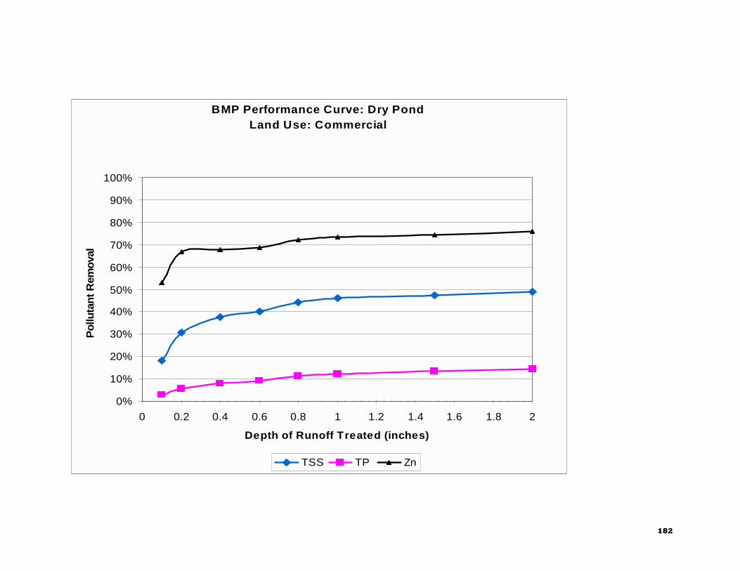
182
BMP Performance Curve: Dry PondLand Use: Commercial
0%
10%
20%
30%
40%
50%
60%
70%
80%
90%
100%
0 0.2 0.4 0.6 0.8 1 1.2 1.4 1.6 1.8 2
Depth of Runoff Treated (inches)
Po
lluta
nt
Rem
ova
l
TSS TP Zn

BMP Performance Curve: Dry Pond
183
BMP Performance Curve: Dry PondLand Use: Industrial
0%
10%
20%
30%
40%
50%
60%
70%
80%
90%
100%
0 0.2 0.4 0.6 0.8 1 1.2 1.4 1.6 1.8 2
Depth of Runoff Treated (inches)
Po
lluta
nt R
emo
val
TSS TP Zn
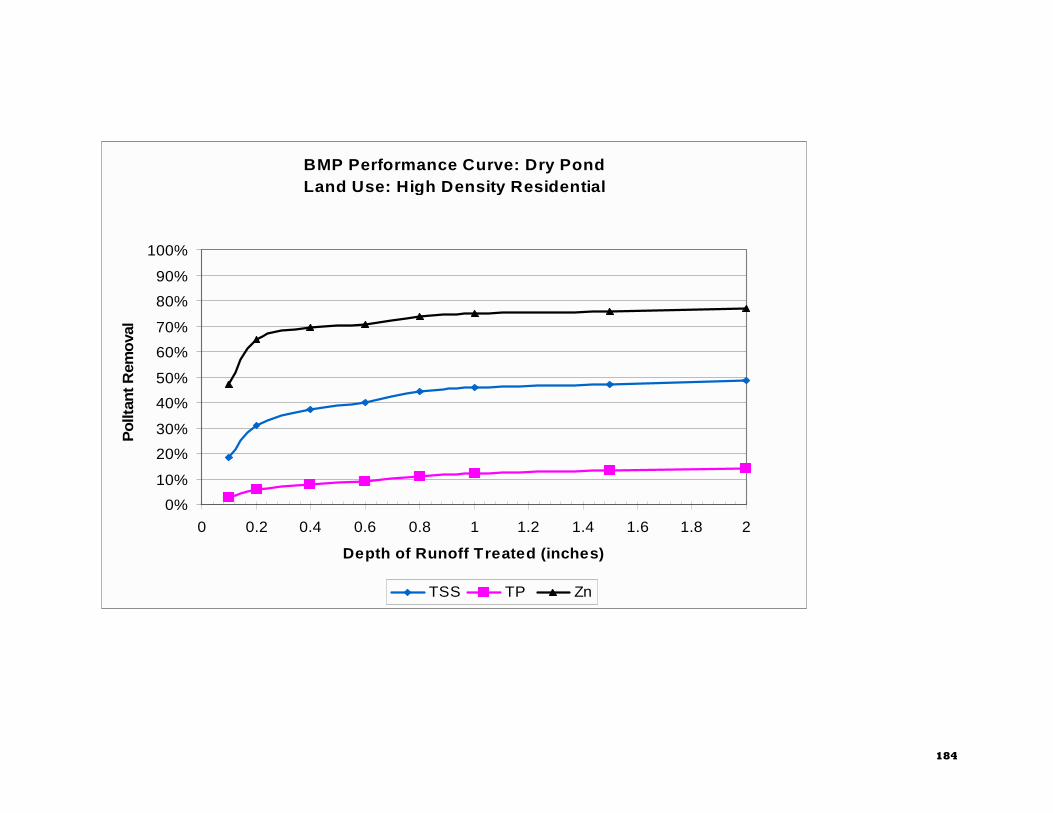
184
BMP Performance Curve: Dry PondLand Use: High Density Residential
0%
10%
20%
30%
40%
50%
60%
70%
80%
90%
100%
0 0.2 0.4 0.6 0.8 1 1.2 1.4 1.6 1.8 2
Depth of Runoff Treated (inches)
Po
lltan
t R
emo
val
TSS TP Zn
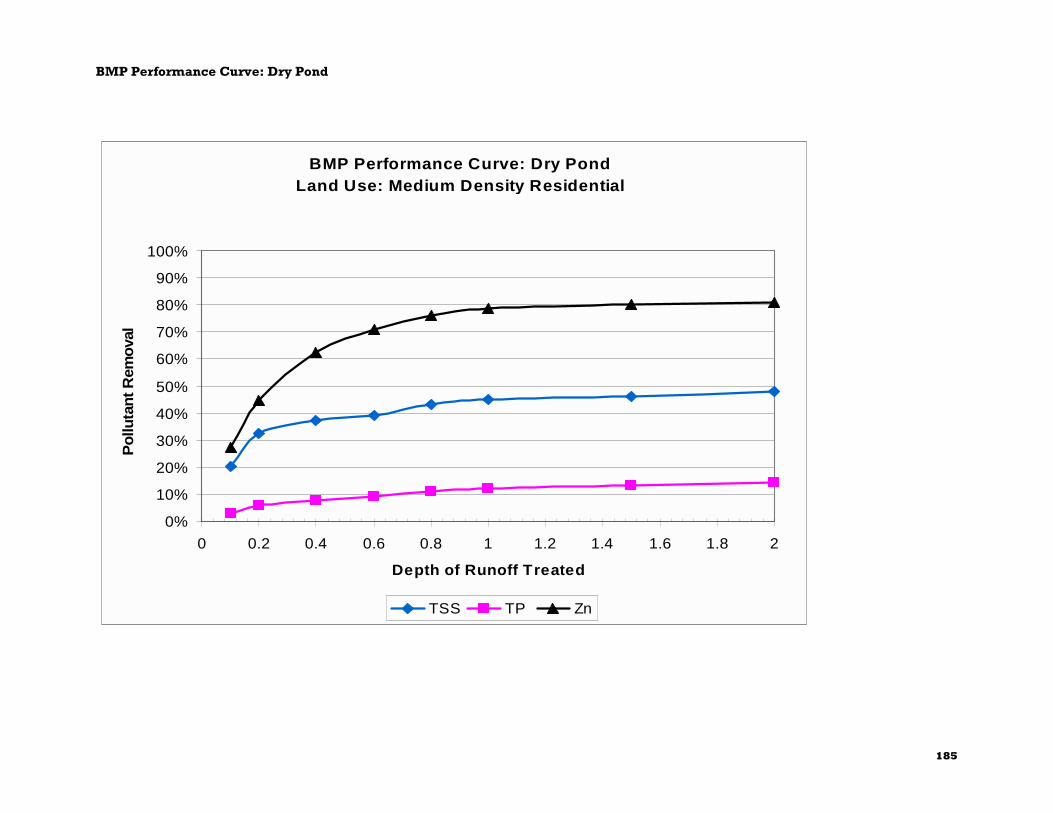
BMP Performance Curve: Dry Pond
185
BMP Performance Curve: Dry PondLand Use: Medium Density Residential
0%
10%
20%
30%
40%
50%
60%
70%
80%
90%
100%
0 0.2 0.4 0.6 0.8 1 1.2 1.4 1.6 1.8 2
Depth of Runoff Treated
Po
lluta
nt
Rem
ova
l
TSS TP Zn

186
BMP Performance Curve: Dry PondLand Use: Low Density Residential
0%
10%
20%
30%
40%
50%
60%
70%
80%
90%
100%
0 0.2 0.4 0.6 0.8 1 1.2 1.4 1.6 1.8 2
Depth of Runoff Treated
Po
lluta
nt
Rem
ova
l
TSS TP Zn

BMP Performance Curve: Porous Pavement
187
BMP Performance Curve: Porous
Pavement
Prepared for: United States Environmental Protection Agency – Region 1 One Congress Street, Suite 1100 Boston, MA 02114 Prepared by: Tetra Tech, Inc. 10306 Eaton Place, Suite 340 Fairfax, VA 22030 September 2008

188
BMP Performance Table BMP Name: Porous Pavement
Depth of Filter Course Layer (inches) Land Use Pollutant
12 18 24 32 TSS 92% 94% 96% 97% TP 62% 69% 74% 78%
Commercial
Zn 85% 97% 97% 98% TSS 92% 94% 96% 98% TP 62% 70% 75% 79%
Industrial
Zn 90% 94% 95% 95% TSS 92% 94% 96% 98% TP 62% 70% 74% 78%
High-Density Residential
Zn 88% 95% 96% 96% TSS 95% 97% 98% 99% TP 61% 68% 73% 77%
Medium-Density Residential
Zn 70% 71% 75% 79% TSS 92% 94% 96% 97% TP 60% 67% 71% 75%
Low-Density Residential
Zn 63% 64% 69% 74%
Annual Pollutant Loading Rates
Pollutant load (lbs/acre-year) Land use TSS TP Zn
Commercial 1117.77 1.66 2.33 Industrial 745.22 1.43 0.45
High-Density Residential 465.08 1.10 0.79 Medium-Density Residential 274.63 0.55 0.11
Low-Density Residential 72.11 0.042 0.043

BMP Performance Curve: Porous Pavement
189
BMP Performance Curve: Porous PavementLand Use: Commercial
0%
10%
20%
30%
40%
50%
60%
70%
80%
90%
100%
12 18 24 30
Depth of Filter Course (inches)
Pollu
tant R
emova
l
TSS TP Zn
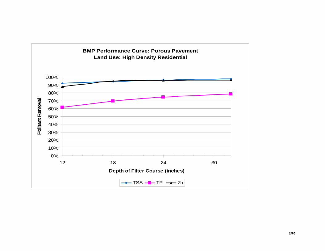
190
BMP Performance Curve: Porous PavementLand Use: High Density Residential
0%
10%
20%
30%
40%
50%
60%
70%
80%
90%
100%
12 18 24 30
Depth of Filter Course (inches)
Pollt
ant R
emova
l
TSS TP Zn

BMP Performance Curve: Porous Pavement
191
BMP Performance Curve: Porous PavementLand Use: Industrial
0%
10%
20%
30%
40%
50%
60%
70%
80%
90%
100%
12 18 24 30
Depth of Filter Course (inches)
Pollu
tan
t Rem
ova
l
TSS TP Zn

192
BMP Performance Curve: Porous PavementLand Use: Medium Density Residential
0%
10%
20%
30%
40%
50%
60%
70%
80%
90%
100%
12 18 24 30
Depth of Filter Course (inches)
Pollu
tant R
emova
l
TSS TP Zn

BMP Performance Curve: Porous Pavement
193
BMP Performance Curve: Porous PavementLand Use: Low Density Residential
0%
10%
20%
30%
40%
50%
60%
70%
80%
90%
100%
12 18 24 30
Depth of Filter Course (inches)
Pollu
tant R
emova
l
TSS TP Zn


