
Stochastic Partial Differential Equations:Analysis and Numerical Approximations
Arnulf Jentzen
May 23, 2016

2
Preface
These lecture notes have been written for the course “401-4606-00L Numerical Anal-ysis of Stochastic Partial Differential Equations” in the spring semester 2014 and inthe spring semester 2015. These lecture notes are far away from being complete andremain under construction. In particular, these lecture notes do not yet contain asuitable comparison of the presented material with existing results, arguments andnotions in the literature. This will be the subject of a future version of these lecturenotes. Furthermore, these lecture notes do not contain a number of proofs, argu-ments and intuitions. For most of this additional material, the reader is referredto the lectures of the course “401-4606-00L Numerical Analysis of Stochastic PartialDifferential Equations” in the spring semester 2014. Sonja Cox and Ryan Kurniawanare gratefully acknowledged for their very helpful advice and assistance, especiallyfor their help with the Matlab programs. Daniel Conus is also gratefully acknowl-edged for several comments that helped to improve the presentation of the results.In addition, we thank Antti Knowles and Benno Kuckuck for fruitful discussions.The students of the course “401-4606-00L Numerical Analysis of Stochastic PartialDifferential Equations” in the spring semester 2014 are gratefully acknowledged forpointing out a number of misprints to me. Special thanks are due to Timo Welti forbringing a number of misprints to my notice.
Zurich, March 2016
Arnulf Jentzen

3
Exercises
Solutions to the exercises can be turned in the designated mailbox in the anteroomHG G 53.x.
Exerc. Exercises Deadlinesheet1 Exerc. 1.1.8, 1.1.9, 1.1.10, & 2.2.6. 17.03.2016, 10:15 AM2 Exerc. 2.3.7, 2.4.20, 2.4.23, 3.4.23, 3.6.4, 3.6.5, & 3.6.18. 07.04.2016, 10:15 AM3 Exerc. 3.6.26, 4.3.3, 4.8.7, & 6.1.20 21.04.2016, 10:15 AM4 Exerc. 6.3.17 28.04.2016, 10:15 AM5 Exerc. 7.1.17 & 7.1.18 12.05.2016, 10:15 AM6 Exerc. 7.2.4 19.05.2016, 10:15 AM7 Exerc. 8.1.6 & 8.1.14 26.05.2016, 10:15 AM8 Exerc. 8.2.3 01.06.2016, 10:15 AM

4

Contents
I Foundations in mathematical analysis 13
1 Gronwall-type inequalities 151.1 Properties of the beta and the gamma function . . . . . . . . . . . . 15
1.1.1 Functional equation of the gamma function . . . . . . . . . . . 161.1.2 Monotonicity properties of the gamma and the beta function . 161.1.3 Estimates for the beta and the gamma function . . . . . . . . 17
1.2 Integral operators related to the beta function . . . . . . . . . . . . . 201.3 Generalized exponential-type functions . . . . . . . . . . . . . . . . . 221.4 Generalized time-continuous Gronwall-type inequalities . . . . . . . . 23
1.4.1 Gronwall-type inequalities with singularities at initial time . . 251.4.2 Gronwall-type inequalities without singularities at initial time 27
2 Nonlinear functions and nonlinear spaces 292.1 Sets and relations . . . . . . . . . . . . . . . . . . . . . . . . . . . . . 29
2.1.1 General functions . . . . . . . . . . . . . . . . . . . . . . . . . 302.1.2 Preordered sets . . . . . . . . . . . . . . . . . . . . . . . . . . 30
2.2 Measurable functions . . . . . . . . . . . . . . . . . . . . . . . . . . . 312.2.1 Nonlinear characterization of the Borel sigma-algebra . . . . . 322.2.2 Pointwise limits of measurable functions . . . . . . . . . . . . 33
2.3 Strongly measurable functions . . . . . . . . . . . . . . . . . . . . . . 342.3.1 Simple functions . . . . . . . . . . . . . . . . . . . . . . . . . 342.3.2 Separability . . . . . . . . . . . . . . . . . . . . . . . . . . . . 342.3.3 Strongly measurable functions . . . . . . . . . . . . . . . . . . 362.3.4 Pointwise approximations of strongly measurable functions . . 372.3.5 Sums of strongly measurable functions . . . . . . . . . . . . . 40
2.4 Continuous functions . . . . . . . . . . . . . . . . . . . . . . . . . . . 412.4.1 Topological spaces . . . . . . . . . . . . . . . . . . . . . . . . 412.4.2 Semi-metric spaces . . . . . . . . . . . . . . . . . . . . . . . . 44
5

6 CONTENTS
2.4.3 Continuity properties of functions . . . . . . . . . . . . . . . . 452.4.4 Modulus of continuity . . . . . . . . . . . . . . . . . . . . . . 462.4.5 Extensions of uniformly continuous functions . . . . . . . . . . 48
3 Linear functions and linear spaces 513.1 Sums over possibly uncountable index sets . . . . . . . . . . . . . . . 51
3.1.1 Cofinal sequences . . . . . . . . . . . . . . . . . . . . . . . . . 513.1.2 Sums over possibly uncountable index sets . . . . . . . . . . . 543.1.3 Fubini for sums . . . . . . . . . . . . . . . . . . . . . . . . . . 54
3.2 Sets of integrable functions . . . . . . . . . . . . . . . . . . . . . . . . 573.2.1 Lp-sets of measurable functions for p P r0,8q . . . . . . . . . . 573.2.2 Lp-spaces of strongly measurable functions for p P r0,8q . . . 58
3.3 Linear spaces . . . . . . . . . . . . . . . . . . . . . . . . . . . . . . . 593.4 Hilbert spaces . . . . . . . . . . . . . . . . . . . . . . . . . . . . . . . 60
3.4.1 Orthonormal bases . . . . . . . . . . . . . . . . . . . . . . . . 603.4.2 Best approximations and projections in Hilbert spaces . . . . 623.4.3 Examples of orthonormal bases . . . . . . . . . . . . . . . . . 63
3.4.3.1 Elementary properties of trigonometric functions . . 633.4.3.2 Orthonormal basis in L2pBorelp0,1q; |¨|Rq . . . . . . . . 653.4.3.3 Transformations of orthonormal bases . . . . . . . . 71
3.5 Linear functions . . . . . . . . . . . . . . . . . . . . . . . . . . . . . . 723.5.1 Continuous linear functions on normed vector spaces . . . . . 733.5.2 Nuclear operators on Banach spaces . . . . . . . . . . . . . . . 75
3.5.2.1 Definition of Nuclear operators . . . . . . . . . . . . 753.5.2.2 Relation of bounded linear operators and nuclear op-
erators . . . . . . . . . . . . . . . . . . . . . . . . . . 763.5.2.3 Structure of the space of nuclear operators . . . . . . 773.5.2.4 Ideal property of the set of nuclear operators . . . . 783.5.2.5 Characterization of nuclear operators . . . . . . . . . 79
3.5.3 Hilbert-Schmidt operators on Hilbert spaces . . . . . . . . . . 793.5.3.1 Independence of the orthonormal basis . . . . . . . . 793.5.3.2 The Hilbert space of Hilbert-Schmidt operators . . . 803.5.3.3 Hilbert-Schmidt embeddings . . . . . . . . . . . . . . 81
3.6 Diagonal linear operators on Hilbert spaces . . . . . . . . . . . . . . . 823.6.1 Laplace operators on bounded domains . . . . . . . . . . . . . 84
3.6.1.1 Laplace operators with Dirichlet boundary conditions 843.6.1.2 Laplace operators with Neumann boundary conditions 863.6.1.3 Laplace operators with periodic boundary conditions 87
CONTENTS 7
3.6.2 Spectral decomposition for a diagonal linear operator . . . . . 88
3.6.3 Fractional powers of a diagonal linear operator . . . . . . . . . 92
3.6.4 Domain Hilbert space associated to a diagonal linear operator 93
3.6.5 Interpolation spaces associated to a diagonal linear operator . 94
3.7 The Bochner integral . . . . . . . . . . . . . . . . . . . . . . . . . . . 96
3.7.1 Existence and uniqueness of the Bochner integral . . . . . . . 96
3.7.2 Definition of the Bochner integral . . . . . . . . . . . . . . . . 97
4 Semigroups of bounded linear operators 99
4.1 Definition of a semigroup of bounded linear operators . . . . . . . . . 99
4.2 Types of semigroups . . . . . . . . . . . . . . . . . . . . . . . . . . . 99
4.3 The generator of a semigroup . . . . . . . . . . . . . . . . . . . . . . 100
4.4 Global a priori bounds for semigroups . . . . . . . . . . . . . . . . . . 101
4.5 Strongly continuous semigroups . . . . . . . . . . . . . . . . . . . . . 102
4.5.1 A priori bounds for strongly continuous semigroups . . . . . . 102
4.5.1.1 The Baire category theorem on complete metric spaces102
4.5.1.2 The uniform boundedness principle . . . . . . . . . . 103
4.5.1.3 Local a priori bounds . . . . . . . . . . . . . . . . . 103
4.5.1.4 Global a priori bounds . . . . . . . . . . . . . . . . . 104
4.5.2 Existence of solutions of linear ordinary differential equationsin Banach spaces . . . . . . . . . . . . . . . . . . . . . . . . . 105
4.5.3 Pointwise convergence in the space of bounded linear operators 106
4.5.4 Domains of generators of strongly continuous semigroups . . . 107
4.5.5 Generators of strongly continuous semigroups . . . . . . . . . 108
4.5.6 A generalization of matrix exponentials to infinite dimensions 111
4.5.7 A characterization of strongly continuous semigroups . . . . . 111
4.6 Uniformly continuous semigroups . . . . . . . . . . . . . . . . . . . . 112
4.6.1 Matrix exponential in Banach spaces . . . . . . . . . . . . . . 113
4.6.2 Continuous invertibility of bounded linear operators in Banachspaces . . . . . . . . . . . . . . . . . . . . . . . . . . . . . . . 115
4.6.3 Generators of uniformly continuous semigroup . . . . . . . . . 116
4.6.4 A characterization result for uniformly continuous semigroups 117
4.6.5 An a priori bound for uniformly continuous semigroups . . . . 118
4.7 The Hille-Yosida theorem . . . . . . . . . . . . . . . . . . . . . . . . 118
4.8 Semigroups generated by diagonal operators . . . . . . . . . . . . . . 125
4.8.1 Smoothing effect of the semigroup . . . . . . . . . . . . . . . . 130
4.8.2 Semigroup generated by the Laplace operator . . . . . . . . . 132

8 CONTENTS
II Foundations in probability theory 135
5 Random variables with values in infinite dimensional spaces 1375.1 General measure and probability spaces . . . . . . . . . . . . . . . . . 137
5.1.1 Uniqueness theorem for measures . . . . . . . . . . . . . . . . 1375.1.2 Independence on probability spaces . . . . . . . . . . . . . . . 1405.1.3 Factorization lemma for conditional expectations . . . . . . . 141
5.2 Borel sigma-algebras on normed vector spaces . . . . . . . . . . . . . 1435.2.1 The Hahn-Banach theorem . . . . . . . . . . . . . . . . . . . . 1435.2.2 Norm representations in normed vector spaces . . . . . . . . . 1445.2.3 Linear characterization of the Borel sigma-algebra . . . . . . . 145
5.3 Probability measures on normed vector spaces . . . . . . . . . . . . . 1465.3.1 Fourier transform of a measure . . . . . . . . . . . . . . . . . 146
5.3.1.1 Characteristic functionals . . . . . . . . . . . . . . . 1465.3.1.2 Fourier transform on separable normed vector spaces 1475.3.1.3 Almost surely separably supported . . . . . . . . . . 1485.3.1.4 Trace set . . . . . . . . . . . . . . . . . . . . . . . . 1495.3.1.5 Fourier transform on normed vector spaces . . . . . . 152
5.3.2 Covariances on normed vector spaces . . . . . . . . . . . . . . 1555.3.2.1 Regularities for correlations on normed vector spaces 1555.3.2.2 Covariances on normed vector spaces . . . . . . . . . 158
5.4 Probability measures on Hilbert spaces . . . . . . . . . . . . . . . . . 1595.4.1 Nuclear operators on Hilbert spaces . . . . . . . . . . . . . . . 159
5.4.1.1 Rank-1 operators on inner product spaces . . . . . . 1605.4.1.2 Traces of nuclear operators . . . . . . . . . . . . . . 1615.4.1.3 Absolute value operators . . . . . . . . . . . . . . . . 162
5.4.2 Covariances on Hilbert spaces . . . . . . . . . . . . . . . . . . 1645.4.3 Karhunen-Loeve expansion . . . . . . . . . . . . . . . . . . . . 167
5.5 Gaussian measures . . . . . . . . . . . . . . . . . . . . . . . . . . . . 1685.5.1 Gaussian measures on normed vector spaces . . . . . . . . . . 168
5.5.1.1 Fourier transform of a Gaussian measure . . . . . . . 1705.5.1.2 Covariance of a Gaussian measure . . . . . . . . . . 170
5.5.2 Gaussian measures on Hilbert spaces . . . . . . . . . . . . . . 1715.5.2.1 Karhunen-Loeve expansion . . . . . . . . . . . . . . 1715.5.2.2 Fourier transform of a Gaussian measure . . . . . . . 1725.5.2.3 Construction of Gaussian measures on Hilbert spaces 1725.5.2.4 Class exercise on Gaussian distributed random variables1765.5.2.5 Karhunen-Loeve expansion for Brownian motion . . 178
CONTENTS 9
6 Stochastic processes 1876.1 Hilbert space valued stochastic processes . . . . . . . . . . . . . . . . 187
6.1.1 Filtrations . . . . . . . . . . . . . . . . . . . . . . . . . . . . . 1876.1.2 Standard Wiener processes . . . . . . . . . . . . . . . . . . . . 1916.1.3 Pseudo inverse . . . . . . . . . . . . . . . . . . . . . . . . . . 194
6.2 Space-time white noise and Brownian sheet . . . . . . . . . . . . . . . 1976.2.1 Derivative of a Brownian sheet . . . . . . . . . . . . . . . . . 197
6.3 Stochastic Integration . . . . . . . . . . . . . . . . . . . . . . . . . . 1986.3.1 Lenglart’s inequality . . . . . . . . . . . . . . . . . . . . . . . 1986.3.2 Modifications and indistinguishability . . . . . . . . . . . . . . 2026.3.3 Predictability . . . . . . . . . . . . . . . . . . . . . . . . . . . 2046.3.4 Construction of the stochastic integral . . . . . . . . . . . . . 2056.3.5 On the density of elementary processes . . . . . . . . . . . . . 2146.3.6 Elementary processes revisited . . . . . . . . . . . . . . . . . . 2196.3.7 Cylindrical Wiener process . . . . . . . . . . . . . . . . . . . . 220
III Stochastic Partial Differential Equations (SPDEs) 223
7 Solutions of SPDEs 2257.1 Existence, uniqueness and properties of mild solutions of SPDEs . . . 225
7.1.1 Mild solutions of SPDEs . . . . . . . . . . . . . . . . . . . . . 2257.1.2 A setting for SPDEs with globally Lipschitz continuous non-
linearities* . . . . . . . . . . . . . . . . . . . . . . . . . . . . . 2277.1.3 A strong perturbation estimate for SPDEs . . . . . . . . . . . 2287.1.4 Uniqueness of mild solutions of SPDEs . . . . . . . . . . . . . 233
7.1.4.1 Uniqueness of predictable mild solutions of SEEs withglobally Lipschitz continuous coefficients . . . . . . . 233
7.1.4.2 Uniqueness of left-continuous mild solutions of SEEswith semi-globally Lipschitz continuous coefficients . 233
7.1.5 Existence and regularity of mild solutions of SPDEs . . . . . . 2377.1.6 A priori bounds for mild solutions of SPDEs . . . . . . . . . . 237
7.1.6.1 A priori bounds . . . . . . . . . . . . . . . . . . . . . 2377.1.6.2 A priori bounds revisited . . . . . . . . . . . . . . . 2387.1.6.3 Strengthened regularity . . . . . . . . . . . . . . . . 240
7.1.7 Temporal-regularity of solution processes of SPDEs . . . . . . 2427.1.8 Existence of continuous solutions . . . . . . . . . . . . . . . . 242
7.2 Examples of SPDEs . . . . . . . . . . . . . . . . . . . . . . . . . . . . 245

10 CONTENTS
7.2.1 Second order SPDEs* . . . . . . . . . . . . . . . . . . . . . . 245
IV Numerical Analysis of SPDEs 251
8 Strong numerical approximations for SPDEs 253
8.1 Spatial spectral Galerkin approximations for SPDEs . . . . . . . . . . 253
8.1.1 Galerkin projections . . . . . . . . . . . . . . . . . . . . . . . 253
8.1.2 Setting . . . . . . . . . . . . . . . . . . . . . . . . . . . . . . . 260
8.1.3 A strong numerical approximation result for spectral Galerkinapproximations of SPDEs . . . . . . . . . . . . . . . . . . . . 260
8.2 Temporal numerical approximations for SPDEs . . . . . . . . . . . . 265
8.2.1 Euler type approximations for SPDEs . . . . . . . . . . . . . . 265
8.2.1.1 Exponential Euler method . . . . . . . . . . . . . . . 265
8.2.1.2 Accelerated exponential Euler method . . . . . . . . 267
8.2.1.3 Linear-implicit Euler method . . . . . . . . . . . . . 268
8.2.1.4 Linear-implicit Crank-Nicolson-Euler method . . . . 269
8.2.2 Nonlinearity-stopped Euler type approximations for SPDEs . . 270
8.2.2.1 Nonlinearity-stopped exponential Euler method . . . 271
8.2.2.2 Nonlinearity-stopped linear-implicit Euler method . . 272
8.2.3 Milstein type approximations for SPDEs . . . . . . . . . . . . 273
8.2.3.1 Exponential Milstein method . . . . . . . . . . . . . 273
8.2.3.2 Linear-implicit Milstein method . . . . . . . . . . . . 274
8.2.3.3 Linear-implicit Crank-Nicolson-Milstein method . . . 276
8.2.4 Strong convergence analysis for exponential Euler approxima-tions . . . . . . . . . . . . . . . . . . . . . . . . . . . . . . . . 277
8.3 Noise approximations for SPDEs . . . . . . . . . . . . . . . . . . . . 288
8.3.1 Noise perturbation estimates . . . . . . . . . . . . . . . . . . . 288
8.3.2 Noise approximations for SPDEs . . . . . . . . . . . . . . . . 289
8.4 Full discretizations for SPDEs . . . . . . . . . . . . . . . . . . . . . . 292
8.4.1 Setting . . . . . . . . . . . . . . . . . . . . . . . . . . . . . . . 292
8.4.2 Full-discrete spectral Galerkin exponential Euler method forSPDEs . . . . . . . . . . . . . . . . . . . . . . . . . . . . . . . 292
8.4.3 Full-discrete spectral Galerkin linear-implicit Euler method forSPDEs . . . . . . . . . . . . . . . . . . . . . . . . . . . . . . . 295
8.4.4 Full-discrete spectral Galerkin nonlinearity-stopped exponen-tial Euler method for SPDEs . . . . . . . . . . . . . . . . . . . 297

CONTENTS 11
8.4.5 Full-discrete spectral Galerkin nonlinearity-stopped linear-implicitEuler method for SPDEs . . . . . . . . . . . . . . . . . . . . . 298
9 Solutions to selected exercises 3039.1 Chapter 2 . . . . . . . . . . . . . . . . . . . . . . . . . . . . . . . . . 303
9.1.1 Solution to Exercise 2.2.6 . . . . . . . . . . . . . . . . . . . . 303

12 CONTENTS

Part I
Foundations inmathematical analysis
13


Chapter 1
Gronwall-type inequalities
This chapter is based on Section 7.1 in Henry [5].
1.1 Properties of the beta and the gamma func-
tion
For completeness we first recall the definition of the gamma function and the betafunction.
Definition 1.1.1 (Gamma function*). We denote by Γ: p0,8q Ñ p0,8q the functionwith the property that for all x P p0,8q it holds that
Γpxq “
ż 8
0
tpx´1q e´t dt (1.1)
and we call Γ the gamma function.
Definition 1.1.2 (Beta function*). We denote by B : p0,8q2 Ñ p0,8q the functionwith the property that for all x, y P p0,8q it holds that
Bpx, yq “
ż 1
0
tpx´1qp1´ tqpy´1q dt (1.2)
and we call B the beta function.
15

16 CHAPTER 1. GRONWALL-TYPE INEQUALITIES
1.1.1 Functional equation of the gamma function
Lemma 1.1.3 (Basic properties of the gamma function and the Beta function*).For all x, y P p0,8q, n P N0 it holds that
Bpx, yq “ Bpy, xq “Γpxq ¨ Γpyq
Γpx` yq“
ż 8
0
tpx´1q
p1` tqpx`yqdt, (1.3)
Γpn` 1q “ n! and Γpx` 1q “ x ¨ Γpxq . (1.4)
Proof of Lemma 1.1.3*. First, observe that the integral transformation theorem en-sures that for all x, y P p0,8q it holds that
Bpx, yq “
ż 1
0
tpx´1qp1´ tqpy´1q dt “
ż 8
1
“
1t
‰px´1q “1´ 1
t
‰py´1q 1t2dt
“
ż 8
1
tp´x´1q“
t´1t
‰py´1qdt “
ż 8
1
tp´x´yq pt´ 1qpy´1q dt
“
ż 8
0
pt` 1qp´x´yq tpy´1qdt “
ż 8
0
tpy´1q
pt` 1qpx`yqdt.
(1.5)
Moreover, note that for all x P p0,8q it holds that
Γpx` 1q “
ż 8
0
tppx`1q´1q e´t dt “ ´
ż 8
0
tx“
´e´t‰
dt
“ ´
ˆ
“
txe´t‰t“8
t“0´ x
ż 8
0
tpx´1q e´t dt
˙
“ x
ż 8
0
tpx´1q e´t dt “ x ¨ Γpxq.
(1.6)
The proof of Lemma 1.1.3 is thus completed.
1.1.2 Monotonicity properties of the gamma and the betafunction
Lemma 1.1.4 (Montonicity property of the gamma function*). It holds that
limxÑ8
Γ1pxq “ 8 (1.7)
and there exists a real number C P p0,8q such that for all x, y P rC,8q with x ď yit holds that Γpxq ď Γpyq.

1.1. PROPERTIES OF THE BETA AND THE GAMMA FUNCTION 17
Proof of Lemma 1.1.4*. Observe that for all x P p0,8q it holds that
Γ1pxq “
ż 8
0
lnptq tpx´1q e´t dt
“
ż 1
0
lnptq tpx´1q e´t dt`
ż e
1
lnptq tpx´1q e´t dt`
ż 8
e
lnptq tpx´1q e´t dt
ě inftPp0,1q
“
lnptq tpx´1q e´t‰
`
ż 8
e
lnptq tpx´1q e´t dt
ě inftPp0,1q
“
lnptq tpx´1q‰
`
ż 8
e
tpx´1q e´t dt.
(1.8)
This proves that
limxÑ8
Γ1pxq ě inftPp0,1q
rlnptq ts ` limxÑ8
ż 8
e
tpx´1q e´t dt “ 8. (1.9)
The proof of Lemma 1.1.4 is thus completed.
Lemma 1.1.5 (Monotonicity of the beta function*). For all x, y, x, y P p0,8q withx ď x and y ď y it holds that
Bpx, yq ď Bpx, yq. (1.10)
Proof of Lemma 1.1.5*. Note that for all θ P p0, 1q, x, x P R with x ď x it holdsthat
θx ď θx. (1.11)
Combining this with Definition 1.1.2 completes the proof of Lemma 1.1.5.
1.1.3 Estimates for terms containing the beta or the gammafunction
Lemma 1.1.6 (An upper bound for the beta function*). Let x, y P p0,8q withpx´ 1q py ´ 1q ě 0. Then
Bpx, yq “
ż 1
0
p1´ tqpx´1q tpy´1q dt ď
ż 1
0
tpx`y´2q dt “
#
8 : x` y ď 11
px`y´1q: x` y ą 1
. (1.12)

18 CHAPTER 1. GRONWALL-TYPE INEQUALITIES
Proof of Lemma 1.1.6*. First, observe that the equalities in (1.12) are clear. It thusremains to prove the inequality in (1.12). For this we assume w.l.o.g. that x` y ą 1,that x ‰ 1 and that y ‰ 1 (otherwise also the inequality in (1.12) is clear). Theassumption that px´ 1q py ´ 1q ě 0 hence shows that px´ 1q py ´ 1q ą 0 and thatpy´1qpx´1q
P p0,8q. Combining this with Holder’s inequality proves that
ż 1
0
p1´ tqpx´1q tpy´1q dt
ď
„ż 1
0
p1´ tqpx´1qr1`py´1qpx´1qs dt
´
r1`py´1qpx´1qs
´1¯
„ż 1
0
tpy´1qr1`px´1qpy´1q s dt
´
r1`px´1qpy´1q s
´1¯
“
„ż 1
0
p1´ tqpx`y´2q dt
´
r1`py´1qpx´1qs
´1¯
„ż 1
0
tpx`y´2q dt
´
r1`px´1qpy´1q s
´1¯
“
ż 1
0
tpx`y´2q dt.
(1.13)
The proof of Lemma 1.1.6 is thus completed.
Remark 1.1.7. Lemma 1.1.6, in particular, shows that for all x, y P p0,8q withpx´ 1q py ´ 1q ě 0 it holds that
Bpx, yq ď
ż 1
0
tpx`y´2q dt. (1.14)
However, it is not true that for all x, y P p0,8q it holds that
Bpx, yq ď
ż 1
0
tpx`y´2q dt. (1.15)
Indeed, observe that
limxŒ0
Bpx, 2´ xq “ limxŒ0
ż 1
0
p1´ tqpx´1q tp2´xq dt ě limxŒ0
ż 1
12
p1´ tqpx´1q tp2´xq dt
ě
„
1
2
p2´xq
limxŒ0
ż 1
12
p1´ tqpx´1q dt “ 8 ą 1 “
ż 1
0
tp2´2q dt.
(1.16)
Exercise 1.1.8 (*). Prove that for all c P r0,8q, ε P p0,8q it holds that
8ÿ
n“1
cn
Γpnεqă 8. (1.17)

1.1. PROPERTIES OF THE BETA AND THE GAMMA FUNCTION 19
Exercise 1.1.9 (*). Prove that for all c P r0,8q, ε P p0,8q it holds that
8ÿ
n“1
cn„
nś
k“1
B`
kε, ε˘
ă 8. (1.18)
Exercise 1.1.10 (*). Prove that for all c P r0,8q, ε, δ, ρ P p0,8q it holds that
8ÿ
n“1
cn„
n´1ś
k“0
B`
ε` kδ, ρ˘
ă 8. (1.19)
Proposition 1.1.11 (Bounds for the gamma function*). It holds for all n P N that
”n
3
ın
ď
”n
e
ın
ă e”n
e
ın
ď n! ď e
„
n` 1
e
n`1
(1.20)
and it holds for all n P N0 that
nn ď en ¨ n! ď pn` 1qpn`1q (1.21)
Proof of Proposition 1.1.11*. Observe that for all n P N0 it holds that
lnpn!q “ ln`
n ¨ pn´ 1q ¨ . . . ¨ 2 ¨ 1˘
“
nÿ
k“1
lnpkq “nÿ
k“1
ż k`1
k
lnpkq dx
ď
nÿ
k“1
ż k`1
k
lnpxq dx “
ż n`1
1
lnpxq dx “ rx lnpxq ´ xsx“n`1x“1
“ pn` 1q lnpn` 1q ´ pn` 1q ` 1 “ pn` 1q lnpn` 1q ´ n.
(1.22)
Moreover, (1.22) ensures for all n P N that
lnpn!q “nÿ
k“1
lnpkq “nÿ
k“2
ż k
k´1
lnpkq dx ěnÿ
k“2
ż k
k´1
lnpxq dx “
ż n
1
lnpxq dx
“ rx lnpxq ´ xsx“nx“1 “ n lnpnq ´ n` 1.
(1.23)
Combining this and (1.22) proves for all n P N that
nn
en´1“ en lnpnq´n`1
ď n! ď epn`1q lnpn`1q´n“pn` 1qpn`1q
en. (1.24)
The proof of Proposition 1.1.11 is thus completed.
20 CHAPTER 1. GRONWALL-TYPE INEQUALITIES
1.2 Integral operators related to the beta function
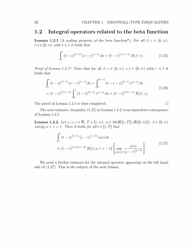
Lemma 1.2.1 (A scaling property of the beta function*). For all β, γ P p0,8q,r, t P r0,8q with r ď t it holds that
ż t
r
pt´ sqpβ´1qps´ rqpγ´1q ds “ pt´ rqpβ`γ´1qBpβ, γq. (1.25)
Proof of Lemma 1.2.1*. Note that for all β, γ P p0,8q, r, t P r0,8q with r ď t itholds that
ż t
r
pt´ sqpβ´1qps´ rqpγ´1q ds “
ż pt´rq
0
pt´ r ´ sqpβ´1q spγ´1q ds
“ pt´ rqpβ`γ´1q
ż 1
0
p1´ sqpβ´1q spγ´1q ds “ pt´ rqpβ`γ´1qBpβ, γq.
(1.26)
The proof of Lemma 1.2.1 is thus completed.
The next estimate, inequality (1.27) in Lemma 1.2.2, is an immediate consequenceof Lemma 1.2.1.
Lemma 1.2.2. Let α, γ, τ P R, T P rτ,8q, u PMpBprτ, T sq,Bpr0,8sqq, β P p0,8qsatisfy α ` γ ą 1. Then it holds for all t P rτ, T s that
ż t
τ
pt´ sqpβ´1qps´ τqpγ´1q upsq ds
ď pt´ τqpα`β`γ´2qB`
β, α ` γ ´ 1˘
«
supsPpτ,tq
upsq
ps´ τqpα´1q
ff
.
(1.27)
We need a further estimate for the integral operator appearing on the left handside of (1.27). This is the subject of the next lemma.
1.2. INTEGRAL OPERATORS RELATED TO THE BETA FUNCTION 21
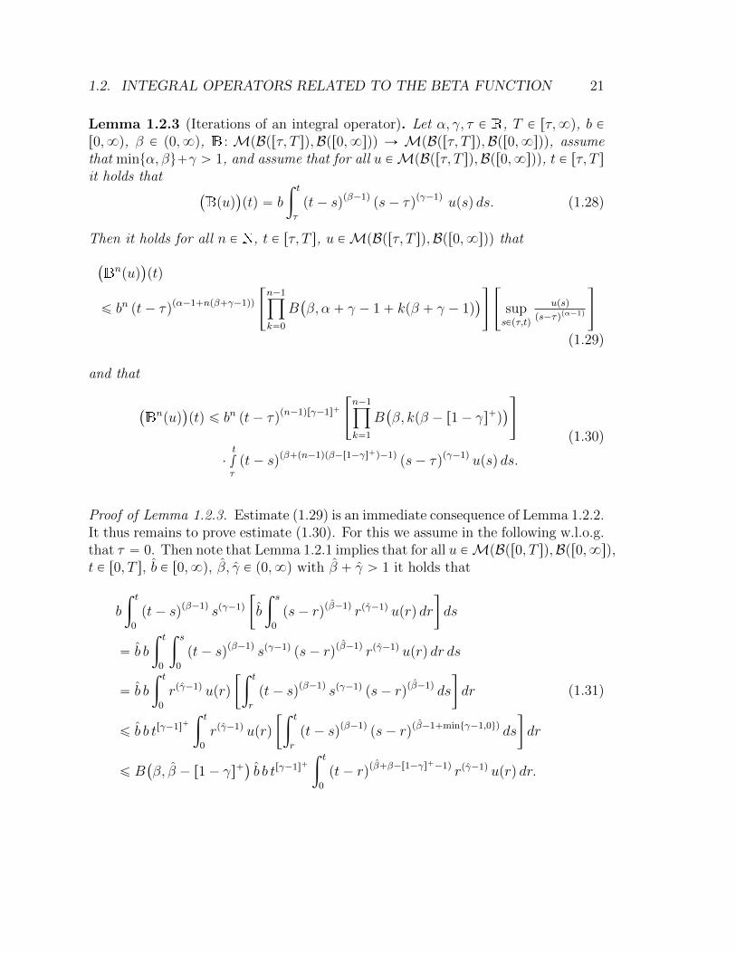
Lemma 1.2.3 (Iterations of an integral operator). Let α, γ, τ P R, T P rτ,8q, b Pr0,8q, β P p0,8q, B : MpBprτ, T sq,Bpr0,8sqq Ñ MpBprτ, T sq,Bpr0,8sqq, assumethat mintα, βu`γ ą 1, and assume that for all u PMpBprτ, T sq,Bpr0,8sqq, t P rτ, T sit holds that
`
Bpuq˘
ptq “ b
ż t
τ
pt´ sqpβ´1qps´ τqpγ´1q upsq ds. (1.28)
Then it holds for all n P N, t P rτ, T s, u PMpBprτ, T sq,Bpr0,8sqq that
`
Bnpuq
˘
ptq
ď bn pt´ τqpα´1`npβ`γ´1qq
«
n´1ź
k“0
B`
β, α ` γ ´ 1` kpβ ` γ ´ 1q˘
ff«
supsPpτ,tq
upsq
ps´τqpα´1q
ff
(1.29)
and that
`
Bnpuq
˘
ptq ď bn pt´ τqpn´1qrγ´1s`
«
n´1ź
k“1
B`
β, kpβ ´ r1´ γs`q˘
ff
¨t
∫τpt´ sqpβ`pn´1qpβ´r1´γs`q´1q
ps´ τqpγ´1q upsq ds.
(1.30)
Proof of Lemma 1.2.3. Estimate (1.29) is an immediate consequence of Lemma 1.2.2.It thus remains to prove estimate (1.30). For this we assume in the following w.l.o.g.that τ “ 0. Then note that Lemma 1.2.1 implies that for all u PMpBpr0, T sq,Bpr0,8sq,t P r0, T s, b P r0,8q, β, γ P p0,8q with β ` γ ą 1 it holds that
b
ż t
0
pt´ sqpβ´1q spγ´1q
„
b
ż s
0
ps´ rqpβ´1q rpγ´1q uprq dr
ds
“ b b
ż t
0
ż s
0
pt´ sqpβ´1q spγ´1qps´ rqpβ´1q rpγ´1q uprq dr ds
“ b b
ż t
0
rpγ´1q uprq
„ż t
r
pt´ sqpβ´1q spγ´1qps´ rqpβ´1q ds
dr
ď b b trγ´1s`ż t
0
rpγ´1q uprq
„ż t
r
pt´ sqpβ´1qps´ rqpβ´1`mintγ´1,0uq ds
dr
ď B`
β, β ´ r1´ γs`˘
b b trγ´1s`ż t
0
pt´ rqpβ`β´r1´γs`´1q rpγ´1q uprq dr.
(1.31)

22 CHAPTER 1. GRONWALL-TYPE INEQUALITIES
Iterating (1.31) shows that for all u PMpBpr0, T sq,Bpr0,8sq, t P r0, T s, n P t2, 3, . . . uit holds that
`
Bnpuq
˘
ptq ď bn tpn´1qrγ´1s`t
∫0pt´ sqpβ`pn´1qpβ´r1´γs`q´1q spγ´1q upsq ds
¨
«
n´1ź
k“1
B`
β, kpβ ´ r1´ γs`q˘
ff
.
(1.32)
The proof of Lemma 1.2.3 is thus completed.
1.3 Generalized exponential-type functions
Definition 1.3.1 (Generalized exponential-type functions*). We denote by Er : r0,8q Ñr0,8q, r P p0,8q, Er : r0,8q Ñ r0,8q, r P p0,8q, and Er : r0,8q Ñ r0,8q,r P p0,8q, the functions with the property that for all r P p0,8q, x P r0,8q itholds that
Errxs “8ÿ
n“0
xnr
Γpnr ` 1q, Errxs “ Er
”
pxΓprqq1r
ı
“
8ÿ
n“0
pxΓprqqn
Γpnr ` 1q(1.33)
and Errxs “b
Errx2s “
«
8ÿ
n“0
px2Γprqqn
Γpnr ` 1q
ff12
. (1.34)
Lemma 1.3.2. Let r P p0,8q, x P r0,8q. Then
8ÿ
n“0
xnr
Γpnr ` 1qďemaxtx,1u maxtx, 1u r1rs1
infsPp0,8q Γpsq. (1.35)
Proof of Lemma 1.3.2. First, observe that
8ÿ
n“0
xnr
Γpnr ` 1q“
8ÿ
k“0
ÿ
nPN0,kďnrăk`1
xnr
Γpnr ` 1q
“ÿ
nPN0,nră1
xnr
Γpnr ` 1q`
8ÿ
k“1
ÿ
nPN0,kďnrăk`1
xnr
Γpnr ` 1q
ďÿ
nPN0,nră1
xnr
infsPp0,8q Γpsq`
8ÿ
k“1
ÿ
nPN0,kďnrăk`1
rmaxtx, 1uspk`1q
Γpk ` 1q.
(1.36)

1.4. GENERALIZED TIME-CONTINUOUS GRONWALL-TYPE INEQUALITIES23
This shows that
8ÿ
n“0
xnr
Γpnr ` 1qď
1
infsPp0,8q Γpsq
»
—
–
8ÿ
k“0
ÿ
nPN0,kďnrăk`1
rmaxtx, 1uspk`1q
Γpk ` 1q
fi
ffi
fl
“maxtx, 1u
infsPp0,8q Γpsq
«
8ÿ
k“0
rmaxtx, 1usk
Γpk ` 1q#N0ptn P N0 : k ď nr ă k ` 1uq
ff
ď#N0ptn P N0 : nr ă 1uqmaxtx, 1u
infsPp0,8q Γpsq
«
8ÿ
k“0
rmaxtx, 1usk
k!
ff
“emaxtx,1u#N0ptn P N0 : n ă 1ruqmaxtx, 1u
infsPp0,8q Γpsq“
maxtx, 1u emaxtx,1u#N0pr0, 1rqq
infsPp0,8q Γpsq.
(1.37)
The proof of Lemma 1.3.2 is thus completed.
1.4 Generalized time-continuous Gronwall-type in-
equalities
Lemma 1.4.1 (Main idea in the proof of the generalized Gronwall inequality). Letτ P R, T P rτ,8q, b P MpBprτ, T s2q,Bpr0,8sqq, a, e P MpBprτ, T sq,Bpr0,8sqq,B : MpBprτ, T sq,Bpr0,8sqq ÑMpBprτ, T sq,Bpr0,8sqq satisfy that for all t P rτ, T s,u PMpBprτ, T sq,Bpr0,8sqq it holds that
`
Bpuq˘
ptq “t
∫τbpt, squpsq ds, (1.38)
and assume that e ď a`Bpeq. Then it holds for all n P N that
e ďn´1ÿ
k“0
Bkpaq `Bn
peq. (1.39)
Proof of Lemma 1.4.1. Estimate (1.39) follows immediately from an iterated applica-tion of the assumption e ď a`Bpeq and from the fact that B is monotone in the sensethat for all u, u P MpBprτ, T sq,Bpr0,8sqq with u ď u it holds that Bpuq ď Bpuq.The proof of Lemma 1.4.1 is thus completed.

24 CHAPTER 1. GRONWALL-TYPE INEQUALITIES
Next we present the generalized Gronwall inequalities. They are modified versionsof the estimates in Section 7.1 in Henry [5].
Theorem 1.4.2. Let τ P R, b P r0,8q, T P rτ,8q, a, e PMpBprτ, T sq,Bpr0,8sqq,β, γ P p0,8q, B : MpBprτ, T sq,Bpr0,8sqq ÑMpBprτ, T sq,Bpr0,8sqq satisfy β ` γ ą
1 andşT
τps´ τqpγ´1q epsq ds ă 8, assume that for all u P MpBprτ, T sq,Bpr0,8sqq,
t P rτ, T s it holds that
pBuqptq “ bt
∫τpt´ sqpβ´1q
ps´ τqpγ´1q upsq ds, (1.40)
and assume that for all t P rτ, T s it holds that
eptq ď aptq ` bt
∫τpt´ sqpβ´1q
ps´ τqpγ´1q epsq ds. (1.41)
Then it holds for all t P rτ, T s that
eptq ď8ÿ
n“0
`
Bnpaq
˘
ptq ď aptq `8ÿ
n“1
bn pt´ τqpn´1qrγ´1s`„
n´1ś
k“1
B`
β, kpβ ´ r1´ γs`q˘
¨t
∫τpt´ sqpβ`pn´1qpβ´r1´γs`q´1q
ps´ τqpγ´1q apsq ds (1.42)
and it holds for all t P pτ, T s, α P p0,8q with α ` γ ą 1 that
eptq ď8ÿ
n“0
`
Bnpaq
˘
ptq ď aptq (1.43)
`
«
supsPpτ,tq
apsq
ps´τqpα´1q
ff
8ÿ
n“1
bn pt´ τqpα´1`npβ`γ´1qq
„
n´1ś
k“0
B`
β, α ` γ ´ 1` kpβ ` γ ´ 1q˘
looooooooooooooooooooooooooooooooooooooooooomooooooooooooooooooooooooooooooooooooooooooon
ă8
.
Proof of Theorem 1.4.2. W.l.o.g. we assume that τ “ 0. Lemma 1.4.1 implies thatfor all n P N0 it holds that
e ď a`Bpaq `B2paq ` . . .`Bn
paq `Bpn`1qpeq “
«
nÿ
k“0
Bkpaq
ff
`Bpn`1qpeq. (1.44)
Next we note that inequality (1.30) in Lemma 1.2.3 together with the assumptionthat @ t P r0, T s :
şt
0spγ´1q epsq ds ă 8 and the fact that
@ c P r0,8q, r P p0,8q : limnÑ8
„
cn
Γppn´ 1qrq
“ 0 (1.45)

1.4. GENERALIZED TIME-CONTINUOUS GRONWALL-TYPE INEQUALITIES25
(see Exercise 1.1.8) implies that for all t P p0, T s it holds that
limnÑ8
`
Bnpeq
˘
ptq
ď limnÑ8
«
bn tβ´1`pn´1qpβ`γ´1qt
∫0spγ´1qepsq ds
«
n´1ź
k“1
B`
β, kpβ ´ r1´ γs`q˘
ffff
ď∫ t0 spγ´1q epsq ds
tγlimnÑ8
«
“
tpβ`γ´1q b‰n
«
n´1ź
k“1
B`
β, kpβ ´ r1´ γs`q˘
ffff
ď∫ t0 spγ´1q epsq ds
tγlimnÑ8
«
“
maxp1,Γpβqq tpβ`γ´1q b‰n
«
n´1ź
k“1
Γpkpβ´r1´γs`qqΓpβ`kpβ´r1´γs`qq
ffff
ď∫ t0 spγ´1q epsq ds
tγ
¨ limnÑ8
«
“
|1` Γpβq ` Γpβ ´ r1´ γs`q|2 tpβ`γ´1q b‰n
Γ`
β ` pn´ 1qpβ ´ r1´ γs`q˘
„
n´2ś
k“1
Γppk`1qpβ´r1´γs`qqΓpβ`kpβ´r1´γs`qq
ff
ď∫ t0 spγ´1q epsq ds
tγ
„
8ś
k“1
Γppk`1qpβ´r1´γs`qqΓpβ`kpβ´r1´γs`qq
¨ limnÑ8
«
“
|1` Γpβq ` Γpβ ´ r1´ γs`q|2 tpβ`γ´1q b‰n
Γ`
pn´ 1qpβ ´ r1´ γs`q˘
ff
“ 0.
(1.46)
This and (1.44) prove the first inequalities in (1.42) and (1.43). Estimate (1.30) inLemma 1.2.3 proves the second inequality in (1.42). Furthermore, estimate (1.29)in Lemma 1.2.3 proves the second inequality in (1.43). Finally, observe that Exer-cise 1.1.10 implies that for all t P pτ, T s it holds that
8ÿ
n“1
bn pt´ τqnpβ`γ´1q
„
n´1ś
k“0
B`
β, α ` γ ´ 1` kpβ ` γ ´ 1q˘
“
8ÿ
n“1
”
b pt´ τqpβ`γ´1qın
„
n´1ś
k“0
B`
β, α ` γ ´ 1` kpβ ` γ ´ 1q˘
ă 8.
(1.47)
The proof of Theorem 1.4.2 is thus completed.
1.4.1 Gronwall-type inequalities with singularities at initialtime
The next result, Corollary 1.4.3, specialises estimate (1.42) in Theorem 1.4.2 to thecase where γ “ 1; see Lemma 7.1.1 in Henry [5].

26 CHAPTER 1. GRONWALL-TYPE INEQUALITIES
Corollary 1.4.3. Let τ P R, b P r0,8q, T P rτ,8q, a, e PMpBprτ, T sq,Bpr0,8sqq,β P p0,8q satisfy
şT
τepsq ds ă 8 and assume that for all t P rτ, T s it holds that
eptq ď aptq ` bt
∫τpt´ sqpβ´1q epsq ds. (1.48)
Then it holds for all t P rτ, T s that
eptq ď aptq ` rΓpβq bs1β
ż t
τ
E1β“
pt´ sq rΓpβq bs1β‰
apsq ds. (1.49)
Proof of Corollary 1.4.3. Inequality (1.42) in Theorem 1.4.2 with γ “ 1 shows thatfor all t P rτ, T s it holds that
eptq ď aptq `
ż t
τ
«
8ÿ
n“1
rΓpβq bsn pt´ sqpnβ´1q
Γpnβq
ff
apsq ds
“ aptq ` rΓpβq bs1β
ż t
τ
«
8ÿ
n“1
“
pt´ sq rΓpβq bs1β‰pnβ´1q
Γpnβq
ff
apsq ds.
(1.50)
Next note that Lemma 1.1.3 shows that for all x P p0,8q it holds that
E1βpxq “8ÿ
n“1
nβxpnβ´1q
Γpnβ ` 1q“
8ÿ
n“1
xpnβ´1q
Γpnβq. (1.51)
Combining this with (1.50) completes the proof of Corollary 1.4.3.
The next result, Corollary 1.4.4, specialises estimate (1.43) in Theorem 1.4.2 tothe case where the function a in Theorem 1.4.2 satisfies aptq “ c tpα´1q for all t P pτ, T sand some c P r0,8q; see Exercise 3 in Henry [5]. Corollary 1.4.4 follows immediatelyfrom (1.43) in Theorem 1.4.2 and from Exercise 1.1.10.
Corollary 1.4.4. Let τ P R, a, b P r0,8q, T P rτ,8q, α, β, γ P p0,8q, a, e P
MpBprτ, T sq,Bpr0,8sqq satisfy mintα, βu ` γ ą 1 andşT
τps´ τqpγ´1q epsq ds ă 8
and assume that for all t P pτ, T s it holds that
eptq ď a pt´ τqpα´1q` b
t
∫τpt´ sqpβ´1q
ps´ τqpγ´1q epsq ds. (1.52)
Then it holds for all t P pτ, T s that
eptq ď a pt´ τqpα´1q8ÿ
n“0
bn pt´ τqnpβ`γ´1q
„
n´1ś
k“0
B`
β, α ` γ ´ 1` kpβ ` γ ´ 1q˘
ă 8.
(1.53)
1.4. GENERALIZED TIME-CONTINUOUS GRONWALL-TYPE INEQUALITIES27
The next result, Corollary 1.4.5, specialises Corollary 1.4.4 to the case γ “ 1; cf.Exercise 4 in Henry [5]. Corollary 1.4.5 follows immediately from Corollary 1.4.4.
Corollary 1.4.5. Let τ P R, T P rτ,8q, e PMpBprτ, T sq,Bpr0,8sqq, a, b P r0,8q,α, β P p0,8q satisfy
şT
τepsq ds ă 8 and assume that for all t P pτ, T s it holds that
eptq ď a pt´ τqpα´1q` b
t
∫τpt´ sqpβ´1q epsq ds. (1.54)
Then it holds for all t P pτ, T s that
eptq ď a pt´ τqpα´1q8ÿ
n“0
bn pt´ τqnβ„
n´1ś
k“0
B`
β, α ` kβ˘
ă 8. (1.55)
1.4.2 Gronwall-type inequalities without singularities at ini-tial time
In the remainder of these lecture notes we will often use the following Gronwall-typeestimate; see Lemma 7.1.1 in Henry [5].
Corollary 1.4.6 (*). Let τ P R, T P rτ,8q, e PMpBprτ, T sq,Bpr0,8sqq, β P p0,8q,a, b P r0,8q satisfy
şT
τepsq ds ă 8 and assume for all t P rτ, T s that
eptq ď a` bt
∫τpt´ sqpβ´1q epsq ds. (1.56)
Then it holds for all t P rτ, T s that
eptq ď a ¨ Eβ
”
pt´ τq pbΓpβqq1βı
“ a ¨ Eβ
“
pt´ τqβ b‰
. (1.57)
Proof of Corollary 1.4.6. Corollary 1.4.3 implies that for all t P rτ, T s it holds that
eptq ď a` rΓpβq bs1β
ż t
τ
E1β“
pt´ sq rΓpβq bs1β‰
a ds. (1.58)
The fundamental theorem of calculus hence shows that for all t P rτ, T s it holds that
eptq ď a
„
1` limεŒ0
ż t
τ`ε
rΓpβq bs1β E1β
“
ps´ τq rΓpβq bs1β‰
ds
“ a
„
1` limεŒ0
“
Eβ
“
pt´ τq rΓpβq bs1β‰
´ Eβ
“
ε rΓpβq bs1≉
“ a“
1``
Eβ
“
pt´ τq rΓpβq bs1β‰
´ Eβ
“
0‰˘‰
“ aEβ
“
pt´ τq rΓpβq bs1β‰
.
(1.59)
The proof of Corollary 1.4.6 is thus completed.

28 CHAPTER 1. GRONWALL-TYPE INEQUALITIES
Chapter 2
Nonlinear functions and nonlinearspaces
Most of this chapter is based on Da Prato & Zabczyk [3] and Prevot & Rockner [18].
2.1 Sets and relations
Definition 2.1.1 (Power set*). Let A be a set. Then we denote by PpAq the powerset of A (the set of all subsets of A).
Definition 2.1.2 (Sets of numbers*). We denote by
N “ t1, 2, 3, . . . u (2.1)
the set of natural numbers, we denote by
N0 “ NY t0u “ t0, 1, 2, . . . u (2.2)
the union of t0u and the set of natural numbers, we denote by
Z “ t0, 1,´1, 2,´2, . . . u (2.3)
the set of integer numbers, we denote by Q the set of rational numbers, we denoteby R the set of real numbers and we denote by C the set of complex numbers.
Note that Definition 2.1.2, in particular, ensures that N Ă N0 Ă Z Ă Q Ă R Ă
C. For completeness we recall the notion of a relation in the following definition,
29

30 CHAPTER 2. NONLINEAR FUNCTIONS AND NONLINEAR SPACES
Definition 2.1.3. Definition 2.1.3 is used in Subsection 2.1.1 below to recall the notionof a function.
Definition 2.1.3 (Relation*). Let A, B, and C be sets with the property that C ĎpAˆBq. Then and only then we say that pA,B,Cq is a relation (we say that pA,B,Cqis a relation on pA,Bq).
Definition 2.1.4 (*). Let „ “ pA,B,Cq be a relation, let a P A, and let b P B.Then we write a „ b if and only if pa, bq P C.
2.1.1 General functions
Definition 2.1.5 (Function*). Let pA,B,Cq be a relation with the property that forevery a P A there exists exactly one b P B such that pa, bq P C. Then and only thenwe say that pA,B,Cq is a function (we say that pA,B,Cq is a function from A toB).
Definition 2.1.6 (Set of functions*). Let A and B be sets. Then we denote byMpA,Bq the set of all functions from A to B.
Definition 2.1.7 (Domain of definition, codomain, image of a function*). Let Aand B be sets and let f PMpA,Bq. Then
(i) we denote by Dpfq the set given by Dpfq “ A and we call Dpfq the domain ofdefinition of f ,
(ii) we denote by codomainpfq the set given by codomainpfq “ B and we callcodomainpfq the codomain of f ,
(iii) we denote by impfq the set given by impfq “ fpAq “ tfpxq P B : x P Au andwe call impfq the image of f , and
(iv) we denote by graphpfq the set given by graphpfq “ tpx, yq P AˆB : y “ fpxquand we call graphpfq the graph of f .
2.1.2 Preordered sets
Definition 2.1.8 (Preordered set*). Let X be a set and let ĺ be a relation on pX,Xqwith the property that
(i) @x P X : x ĺ x (Reflexivity) and
(ii) @x, y, z P X :`
px ĺ y and y ĺ zq ñ px ĺ zq˘
(Transitivity).
Then and only then we say that pX,ĺq is a preordered set.

2.2. MEASURABLE FUNCTIONS 31
Definition 2.1.9 (Partially ordered set*). Let pX,ĺq be a preorder with the propertythat for all A,B P X with A ĺ B and B ĺ A it holds that A “ B (Antisymmetry).Then and only then we say that pX,ĺq is a partially ordered set.
Definition 2.1.10 (Directed set*). Let pX,ĺq be a preorder with the property that
@x, y P X : D z P X : px ĺ z and y ĺ zq . (2.4)
Then and only then we say that pX,ĺq is a directed set.
Definition 2.1.11 (Nets*). Let pX,ĺq be a directed set, let pE, Eq be a topologicalspace, and let φ : X Ñ E be a function from X to E. Then and only then we saythat φ is a net (we say that φ is a net from pX,ĺq to pE, Eq).
Definition 2.1.12 (Convergence of a net*). Let pX,ĺq be a directed set, let pE, Eqbe a topological space, let e P E, and let φ : X Ñ E be a net. Then we write
limxPpX,ĺq
φpxq “ e (2.5)
and we say that φ converges to e (we say that φ converges to e with respect to pX,ĺq)if and only if for every neighbourhood U Ď E of e there exists a y P X such that forall x P X with y ĺ x it holds that φpxq P U .
2.2 Measurable functions
We first recall the notion of a measurable mapping.
Definition 2.2.1 (Measurable functions*). Let pΩ1,F1q and pΩ2,F2q be measurablespaces and let f : Ω1 Ñ Ω2 be a function with the property that for all F P F2 it holdsthat
f´1pF q P F1. (2.6)
Then and only then we say that f is F1/F2-measurable.
Definition 2.2.2 (Set of all measurable functions*). Let pΩ1,F1q and pΩ2,F2q bemeasurable spaces. Then we denote by MpF1,F2q the set of all F1/F2-measurablefunctions.
Definition 2.2.3 (Borel sigma-algebra*). Let pE, Eq be a topological space. Thenwe denote by BpEq the set given by BpEq “ σEpEq and we call BpEq the Borelsigma-algebra on pE, Eq.

32 CHAPTER 2. NONLINEAR FUNCTIONS AND NONLINEAR SPACES
2.2.1 Nonlinear characterization of the Borel sigma-algebra
Proposition 2.2.5 below demonstrates that if pE, dq is a metric space, then BpEq is thesmallest sigma-algebra with the property that every continuous real-valued functionis Borel measurable. We refer to the statement of Proposition 2.2.5 as nonlinearcharacterization of the Borel sigma-algebra. In the proof of Proposition 2.2.5 we usethe following notation.
Definition 2.2.4 (Distance of sets*). Let pE, dq be a metric space. Then we denoteby distd : PpEq ˆ PpEq Ñ r0,8s the function with the property that for all A,B P
PpEq it holds that
distdpA,Bq “
#
infaPA infbPB dpa, bq : A ‰ H and B ‰ H
8 : else. (2.7)
We now present the promised nonlinear characterization result for Borel sigma-algebras for metric spaces.
Proposition 2.2.5 (Nonlinear characterization of the Borel sigma-algebra*). LetpE, dq be a metric space. Then
BpEq “ σE`
pϕqϕPCpE,Rq˘
“ σEpϕ : ϕ P CpE,Rqq
“ σE`
ϕ´1pAq P PpEq : ϕ P CpE,Rq, A P BpRq
(˘
.(2.8)
Proof of Proposition 2.2.5*. First of all, observe that for every ϕ P CpE,Rq it holdsthat ϕ is BpEq/BpRq-measurable. Hence, we obtain that
BpEq Ě σE`
ϕ´1pAq P PpEq : ϕ P CpE,Rq, A P BpRq
(˘
. (2.9)
It thus remains to prove that
BpEq Ď σE`
ϕ´1pAq P PpEq : ϕ P CpE,Rq, A P BpRq
(˘
. (2.10)
For this observe by that definition it holds that
BpEq “ σEptA P PpEq : A is an open set in pE, dquq . (2.11)
It thus remains to prove that
tA P PpEq : A is an open set in pE, dqu
Ď σE`
ϕ´1pAq P PpEq : ϕ P CpE,Rq, A P BpRq
(˘
.(2.12)
2.2. MEASURABLE FUNCTIONS 33
For this let B Ă E be an open set in pE, dq and let ψ : E Ñ R be the function withthe property that for all x P E it holds that
ψpxq “ distdptxu, EzBq. (2.13)
Observe that ψ P CpE,Rq. This implies that
B “ ψ´1pp0,8qq Ď σE
`
ϕ´1pAq P PpEq : ϕ P CpE,Rq, A P BpRq
(˘
. (2.14)
The proof of Proposition 2.2.5 is thus completed.
Exercise 2.2.6 (*). Let pΩ,Fq be a measurable space, let pE, dq be a metric space,and let f : Ω Ñ E be a function. Prove that f is F/BpEq-measurable if and only ifit holds for all ϕ P CpE,Rq that ϕ ˝ f is F/BpRq-measurable.
2.2.2 Pointwise limits of measurable functions
Lemma 2.2.7 (*). Let pΩ,Fq be a measurable space, let Y : Ω Ñ R be a function,and let Xn : Ω Ñ R, n P N, be a sequence of F/BpRq-measurable mappings such thatfor all ω P Ω it holds that Y pωq “ supnPNXnpωq. Then Y is F/BpRq-measurable.
Proof of Lemma 2.2.7*. Note that for all c P R it holds that
tY ď cu “
"
supnPN
Xn ď c
*
“č
nPN
tXn ď culoooomoooon
PF
P F . (2.15)
The proof of Lemma 2.2.7 is thus completed.
Lemma 2.2.8 (*). Let pΩ,Fq be a measurable space, let Y : Ω Ñ R be a function,and let Xn : Ω Ñ R, n P N, be a sequence of F/BpRq-measurable mappings suchthat for all ω P Ω it holds that lim supnÑ8 |Xnpωq ´ Y pωq| “ 0. Then Y is F/BpRq-measurable.
Proof of Lemma 2.2.8*. Note that Lemma 2.2.7 implies that for all c P R it holdsthat
tY ě cu “!
limnÑ8
Xn ě c)
“
"
lim supnÑ8
Xn ě c
*
“
#
limnÑ8
«
supmPtn,n`1,... u
Xm
ff
ě c
+
“č
nPN
#«
supmPtn,n`1,... u
Xm
ff
ě c
+
looooooooooooooomooooooooooooooon
PF
P F . (2.16)
The proof of Lemma 2.2.8 is thus completed.

34 CHAPTER 2. NONLINEAR FUNCTIONS AND NONLINEAR SPACES
The next corollary is an immediate consequence of Exercise 2.2.6 and Lemma 2.2.8;see, e.g., Proposition E.1 in [1] and Proposition A.1.3 in Prevot & Rockner [18].
Corollary 2.2.9 (*). Let pΩ,Fq be a measurable space, let pE, dq be a metric space,and let f : Ω Ñ E be a function. Then f is F/BpEq-measurable if and only if thereexists a sequence gn : Ω Ñ E, n P N, of F/BpEq-measurable functions such that forall ω P Ω it holds that
lim supnÑ8
dpfpωq, gnpωqq “ 0. (2.17)
2.3 Strongly measurable functions
2.3.1 Simple functions
The idea of the Lebesgue integral for real valued functions is to approximate thefunction by suitable simpler functions and then to define the Lebesgue integral ofthe “complicated” function as the limit of the integrals of the simpler functions. Toperform this procedure we use the following definition.
Definition 2.3.1 (Simple functions*). Let pΩ1,F1q and pΩ2,F2q be measurable spacesand let f : Ω1 Ñ Ω2 be an F1/F2-measurable function with the property that the setfpΩ1q is finite. Then and only then we say that f is F1/F2-simple.
2.3.2 Separability
(Unfortunately) Measurable functions can, in general, not be approximated pointwise(see (2.17) in Corollary 2.2.9) by simple functions; see Theorem 2.3.10 below fordetails. To overcome this difficulty, we introduce the notion of a strongly measurablefunction; see Definition 2.3.6 below. In this notion the following definition is used.
Definition 2.3.2 (Separability*). Let pE, Eq be a topological space with the propertythat there exist an at most countable set A Ď E which satisfies A “ E. Then andonly then we say that E is separable (we say that pE, Eq is separable).
A topological space that is not separable is in a certain sense extremely large.This, in turn, can cause several serious difficulties in the analysis of such spaces. Anexample of a non-separable topological space can be found below. The next lemmaprovides an example for a separable topological space.
Lemma 2.3.3 (*). Let a, b P R with a ă b. Then pCpra, bs,Rq, ¨Cpra,bs,Rqq isseparable.

2.3. STRONGLY MEASURABLE FUNCTIONS 35
Proof of Lemma 2.3.3*. Observe that the set
"
f P Cpra, bs,Rq :
ˆ
Dn P N0 : Dλ0, . . . , λn P Q : @x P ra, bs : fpxq “nř
k“0
λkxk
˙*
(2.18)is a countable dense subset of Cpra, bs,Rq. The proof of Lemma 2.3.3 is thus com-pleted.
In the next lemma we provide a further simple example for a separable topologicalspace.
Lemma 2.3.4 (Trivial topology*). Let X be a set. Then it holds that the pairpX, tX,Huq is a separable topological space.
Proof of Lemma 2.3.4*. Throughout this proof assume w.l.o.g. that X ‰ H and letx P X. Next observe that txu is a finite dense subset of X. The proof of Lemma 2.3.4is thus completed.
Subspaces of separable metric spaces are separable too. This is the subject of thenext lemma.
Lemma 2.3.5 (*). Let pE, dq be a separable metric space and let A Ď E. Then themetric space pA, d|AˆAq is separable.
Proof of Lemma 2.3.5*. W.l.o.g. we assume that A ‰ H. Let penqnPN Ď E be asequence of elements in E such that the set ten P E : n P Nu is dense in E. In thenext step let pfnqnPN Ď A be a sequence of elements in A such that for all n P N itholds that
dpfn, enq ď
#
0 : en P A
distdpA, tenuq `1
2n: en R A
. (2.19)

36 CHAPTER 2. NONLINEAR FUNCTIONS AND NONLINEAR SPACES
Next observe that for all v P Aztem P E : m P Nu, n P N it holds that
distdptvu, tf1, f2, . . . uq ď distdptvu, tfn, fn`1, . . . uq
“ infmPtn,n`1,... u
dpv, fmq
ď infmPtn,n`1,... u
rdpv, emq ` dpem, fmqs
ď infmPtn,n`1,... u
„
dpv, emq ` distdpA, temuq `1
2m
ď infmPtn,n`1,... u
„
2 dpv, emq `1
2m
ď 2
„
infmPtn,n`1,... u
dpv, emq
`1
2n
“ 2 distdptvu, ten, en`1, . . . uq `1
2n“
1
2n.
(2.20)
Combining this with the fact that @ v P AXtem : m P Nu : distdptvu, tf1, f2, . . . uq “ 0ensures that the set tfn P A : n P Nu is dense in A. The proof of Lemma 2.3.5 isthus completed.
2.3.3 Strongly measurable functions
Definition 2.3.6 (Strongly measurable functions*). Let pΩ,Fq be a measurablespace, let pE, dq be a metric space, and let f : Ω Ñ E be an F/BpEq-measurablefunction with the property that pfpΩq, d|fpΩqˆfpΩqq is separable. Then and only thenwe say that f is strongly F/pE, dq-measurable (we say that f is strongly measurable).
Let pΩ,Fq be a measurable space and let pE, dq be a separable metric space.Lemma 2.3.5 then shows that for every F/BpEq-measurable mapping f : Ω Ñ E itholds that f is also strongly F/pE, dq-measurable.
Exercise 2.3.7 (*). Give an example of a measurable space pΩ,Fq, of a metricspace pE, dEq, and of an F/BpEq-measurable function f : Ω Ñ E which is notstrongly F/pE, dEq-measurable. Prove that f is F/BpEq-measurable but not stronglyF/pE, dEq-measurable.

2.3. STRONGLY MEASURABLE FUNCTIONS 37
2.3.4 Pointwise approximations of strongly measurable func-tions
As mentioned above, measurable functions can, in general, not be approximatedpointwise by simple functions. However, strongly measurable functions can be ap-proximated pointwise by simple functions. This is the subject of the Theorem 2.3.10below (cf., e.g., Lemma 1.1 in Da Prato & Zabczyk [3] and Lemma A.1.4 in Prevot& Rockner [18]). In the proof of Theorem 2.3.10 the following two lemmas are used.
Lemma 2.3.8 (Projections in metric spaces*). Let pE, dq be a metric space, letn P N, e1, . . . , en P E, and let Ppe1,...,enq : E Ñ E be the function with the propertythat for all x P E it holds that
Ppe1,...,enqpxq “ emintkPt1,2,...,nu : dpek,xq“distdptxu,te1,...,enuqu. (2.21)
Then
(i) it holds that Ppe1,...,enq is BpEq/PpEq-measurable and
(ii) it holds for all x P E that
dpx, Ppe1,...,enqpxqq “ distdptxu, te1, . . . , enuq. (2.22)
Proof of Lemma 2.3.8*. Identity (2.22) is an immediate consequence of (2.21). LetD “ pD1, . . . , Dnq : E Ñ Rn be the function with the property that for all x P E itholds that
Dpxq “ pD1pxq, . . . , Dnpxqq “ pdpx, e1q, . . . , dpx, enqq . (2.23)
Observe that D is continuous and hence that D is BpEq/BpRnq-measurable. This
38 CHAPTER 2. NONLINEAR FUNCTIONS AND NONLINEAR SPACES
implies that for all k P t1, 2, . . . , nu it holds that
P´1pe1,...,enq
ptekuq “
x P E : Ppe1,...,enqpxq “ ek(
“
!
x P E : k “ min
l P t1, 2, . . . , nu : dpel, xq “ distdptxu, te1, . . . , enuq(
)
“
"
x P E : k “ min
"
l P t1, 2, . . . , nu : Dlpxq “ minuPt1,...,nu
Dupxq
**
“
"
x P E :
ˆ
Dkpxq ď minuPt1,...,nu
Dupxq and Dkpxq ă minuPt1,...,k´1u
Dupxq
˙*
“
"
x P E :
ˆ
@ l P t1, . . . , k ´ 1u : Dkpxq ă Dlpxq and@ l P t1, . . . , nu : Dkpxq ď Dlpxq
˙*
“
»
—
–
k´1č
l“1
tx P E : Dkpxq ă Dlpxquloooooooooooooomoooooooooooooon
PBpEq
fi
ffi
fl
č
»
—
–
nč
l“1
tx P E : Dkpxq ď Dlpxquloooooooooooooomoooooooooooooon
PBpEq
fi
ffi
fl
P BpEq.
(2.24)
This, in turn, implies that for all A P PpEq it holds that
P´1pe1,...,enq
pAq “ P´1pe1,...,enq
`
AX te1, . . . , enu˘
“ YfPAXte1,...,enu P´1pe1,...,enq
ptfuqlooooooomooooooon
PBpEq
P BpEq. (2.25)
The proof of Lemma 2.3.8 is thus completed.
Lemma 2.3.9 (*). Let pΩ,Fq be a measurable space, let pE, dq be a metric space,let f : Ω Ñ E be a function, and let gn : Ω Ñ E, n P N, be a sequence of stronglyF/pE, dq-measurable functions such that for all ω P Ω it holds that
lim supnÑ8
dpfpωq, gnpωqq “ 0. (2.26)
Then f is strongly F/pE, dq-measurable.
Proof of Lemma 2.3.9*. Corollary 2.2.9 ensures that f is F/BpEq-measurable. Itthus remains to prove that fpΩq is separable. This follows from Lemma 2.3.5 andfrom the fact that YnPNgnpΩq is separable. The proof of Lemma 2.3.9 is thus com-pleted.
We now present the promised pointwise approximation result for strongly mea-surable functions.

2.3. STRONGLY MEASURABLE FUNCTIONS 39
Theorem 2.3.10 (Approximations of strongly measurable functions*). Let pΩ,Fqbe a measurable space, let pE, dq be a metric space, and let f : Ω Ñ E be a function.Then the following four statements are equivalent:
(i) It holds that f is strongly F/pE, dq-measurable.
(ii) There exists a sequence gn : Ω Ñ E, n P N, of strongly F/pE, dq-measurablefunctions with the property that for all ω P Ω it holds that
lim supnÑ8
dpfpωq, gnpωqq “ 0. (2.27)
(iii) There exists a sequence gn : Ω Ñ E, n P N, of F/BpEq-simple functions withthe property that for all ω P Ω it holds that
lim supnÑ8
dpfpωq, gnpωqq “ 0. (2.28)
(iv) There exists a sequence gn : Ω Ñ E, n P N, of F/BpEq-simple functions withthe property that for all ω P Ω it holds that dpfpωq, gnpωqq P r0,8q, n P N,decreases monotonically to zero.
Proof of Theorem 2.3.10*. Throughout this proof assume w.l.o.g. thatE ‰ H. Clearly,it holds that ((iv) ñ (iii)) and ((iii) ñ (ii)). Lemma 2.3.9 shows that ((ii) ñ (i)).It thus remains to prove that ((i) ñ (iv)). For this let f : Ω Ñ E be a stronglyF/pE, dq-measurable function. The fact that f is strongly F/pE, dq-measurable en-sures that fpΩq is separable. Hence, there exists a sequence penqnPN Ď fpΩq ofelements in fpΩq with the property that
ten P fpΩq : n P Nu Ě fpΩq. (2.29)
In the next step let Ppe1,...,enq : E Ñ E, n P N, and gn : Ω Ñ E, n P N, be thefunctions with the property that for all x P E, n P N it holds that
Ppe1,...,enqpxq “ emintkPt1,2,...,nu : dpek,xq“distdptxu,te1,...,enuqu (2.30)
andgn “ Ppe1,...,enq ˝ f. (2.31)
Lemma 2.3.8 and the fact that f is F/BpEq-measurable implies that for all n P N itholds that gn is F/BpEq-measurable. In addition, by definition it holds for all n P Nthat gnpΩq Ď te1, . . . , enu is a finite set. We hence get that for all n P N it holds

40 CHAPTER 2. NONLINEAR FUNCTIONS AND NONLINEAR SPACES
that gn is an F/BpEq-simple function. Moreover, note that (2.22) in Lemma 2.3.8ensures that for all ω P Ω, n P N it holds that
dpfpωq, gnpωqq “ d`
fpωq, Ppe1,...,enqpfpωqq˘
“ distdptfpωqu, te1, . . . , enuq . (2.32)
This and the fact that @ω P Ω: distdpfpωq, te1, e2, . . . uq “ 0 imply that for all ω P Ω,n P N it holds that
dpfpωq, gnpωqq ě dpfpωq, gn`1pωqq and lim supnÑ8
dpfpωq, gnpωqq “ 0. (2.33)
The proof of Theorem 2.3.10 is thus completed.
2.3.5 Sums of strongly measurable functions
The next result, Corollary 2.3.11, shows that the sum of two strongly measurablemappings is again a strongly measurable mapping. Corollary 2.3.11 follows immedi-ately from Theorem 2.3.10.
Corollary 2.3.11 (*). Let pΩ,Fq be a measurable space, let K P tR,Cu, let pV, ¨V qbe a normed K-vector space, and let f, g : Ω Ñ V be strongly F/pV, ¨V q-measurablemappings. Then f ` g : Ω Ñ V is strongly F/pV, ¨V q-measurable.
Class exercise 2.3.12 (*). The statement of Lemma 2.3.13 is in general not correct.Specify the mistake in the proof of Lemma 2.3.13.
Lemma 2.3.13 (*). Let pΩ,Fq be a measurable space, let pV, ¨V q be an R-Banachspace, let X, Y : Ω Ñ V be F/BpV q-measurable mappings, and let Z : Ω Ñ V be thefunction with the property that for all ω P Ω it holds that Zpωq “ Xpωq`Y pωq. Thenit holds that Z is F/BpV q-measurable.

2.4. CONTINUOUS FUNCTIONS 41
Proof of Lemma 2.3.13*. Throughout this proof let p : V ˆ V Ñ V be the functionwith the property that for all v, w P V it holds that
ppv, wq “ v ` w (2.34)
and let X : Ω Ñ V ˆ V be the function with the property that for all ω P Ω it holdsthat
Xpωq “ pXpωq, Y pωqq. (2.35)
Next observe that p : V ˆ V Ñ V is a continuous function from V ˆ V to V . This,in particular, ensures that p is a measurable function. Moreover, note that theassumption that X and Y are measurable ensures that X : Ω Ñ V ˆ V is alsomeasurable. This and the fact that p : V ˆ V Ñ V is measurable prove that thecomposition function p ˝ X : Ω Ñ V is measurable. Combining this with the factthat
Z “ p ˝X (2.36)
completes the proof of Lemma 2.3.13.
2.4 Continuous functions
2.4.1 Topological spaces
Definition 2.4.1 (Topology*). Let E be a set and let E Ď PpEq be a set
(i) such that H, E P E,
(ii) such that for all A Ď E it holds that YAPAA P E, and
(iii) such that for all A,B P E it holds that pAXBq P E.
Then and only then we say that E is a topology on E (we say that E is a topology).
Definition 2.4.2 (Topological space*). Let E be a set and let E be a topology on E.Then and only then we say that pE, Eq is a topological space.
Proposition 2.4.3 (Topology induced by a function*). Let E be a set, let T Ď Rbe a set, and let d : E ˆ E Ñ T be a function. Then it holds that the set
"
A P PpEq :´
@ v P A :“
D ε P p0,8q : tu P E : dpv, uq ă εu Ď A‰
¯
*
(2.37)
is a topology on E.

42 CHAPTER 2. NONLINEAR FUNCTIONS AND NONLINEAR SPACES
Proof of Proposition 2.4.3*. Throughout this proof let E Ď PpEq be the set givenby
E “"
A P PpEq :´
@ v P A :“
D ε P p0,8q : tu P E : dpv, uq ă εu Ď A‰
¯
*
. (2.38)
First, we observe thatH, E P E . Next we note that for all A Ď E and all v P rYAPAAsthere exists a set A P A and a real number ε P p0,8q such that v P A and such thattu P E : dpv, uq ă εu Ď A. In particular, this implies that for all A Ď E and allv P rYAPAAs there exists a real number ε P p0,8q such that tu P E : dpv, uq ă εu ĎrYAPAAs. Hence, we obtain that for all A Ď E it holds that
rYAPAAs P E . (2.39)
In the next step we observe that for all A,B P E and all v P pAXBq there existsreal numbers εA, εB P p0,8q such that
tu P E : dpv, uq ă εAu Ď A and tu P E : dpv, uq ă εBu Ď B. (2.40)
Hence, we obtain that for all A,B P E and all v P pAXBq there exists real numbersεA, εB P p0,8q such that
u P E : dpv, uq ă mintεA, εBu(
Ď pAXBq . (2.41)
This proves that for all A,B P E it holds that pAXBq P E . The proof of Proposi-tion 2.4.3 is thus completed.
Proposition 2.4.3 above ensures that the designation in the next definition isreasonable.
Definition 2.4.4 (Topology induced by a function*). Let E be a set, let T Ď R bea set, and let d : E ˆ E Ñ T be a function. Then we denote by τpdq Ď PpEq the setgiven by
τpdq “
"
A P PpEq :´
@ v P A :“
D ε P p0,8q : tu P E : dpv, uq ă εu Ď A‰
¯
*
(2.42)
and we call τpdq the topology induced by d.
Lemma 2.4.5 (Balls are open*). Let E be a set, let T Ď R be a set, let d : EˆE Ñ Tbe a function with the property that @x, y, z P E : dpx, zq ď dpx, yq ` dpy, zq, and letε P p0,8q, v P E. Then it holds that
tu P E : dpv, uq ă εu P τpdq. (2.43)

2.4. CONTINUOUS FUNCTIONS 43
Proof of Lemma 2.4.5*. First, observe that for all x P tu P E : dpv, uq ă εu, y P tu PE : dpx, uq ă ε´ dpv, xqu it holds that
dpv, yq ď dpv, xq ` dpx, yq ă dpv, xq ` rε´ dpv, xqs “ ε. (2.44)
This ensures that for all x P tu P E : dpv, uq ă εu it holds that
tu P E : dpx, uq ă ε´ dpv, xqu Ď tu P E : dpv, uq ă εu (2.45)
Hence, we obtain that for all x P tu P E : dpv, uq ă εu there exists a real numberδ P p0,8q such that
tu P E : dpx, uq ă δu Ď tu P E : dpv, uq ă εu . (2.46)
This completes the proof of Lemma 2.4.5.
Proposition 2.4.6 (Convergence in the induced topology*). Let E be a set, letd : E ˆ E Ñ r0,8q be a function with the property that @x P E : dpx, xq “ 0 and@x, y, z P E : dpx, zq ď dpx, yq ` dpy, zq, and let e : N0 Ñ E be a function. Then itholds that
lim supnÑ8
d`
ep0q, epnq˘
“ 0 (2.47)
if and only if for every A P τpdq with ep0q P A there exists a natural number N P N
such that for all n P tN,N ` 1, . . . u it holds that epnq P A.
Proof of Proposition 2.4.6*. First of all, recall that lim supnÑ8 d`
ep0q, epnq˘
“ 0 ifand only if
@ ε P p0,8q : DN P N : @n P tN,N ` 1, . . . u : d`
ep0q, epnq˘
ă ε. (2.48)
Hence, we obtain that lim supnÑ8 d`
ep0q, epnq˘
“ 0 if and only if for all ε P p0,8qthere exists a natural number N P N such that for all n P tN,N ` 1, . . . u it holdsthat epnq P tu P E : dpep0q, uq ă εu. This and Lemma 2.4.5 complete the proof ofProposition 2.4.6.

44 CHAPTER 2. NONLINEAR FUNCTIONS AND NONLINEAR SPACES
2.4.2 Semi-metric spaces
Definition 2.4.7 (Semi-metric*). Let E be a set and let d : E ˆ E Ñ r0,8q be afunction with the property that for all x, y, z P E it holds that
(i) dpx, xq “ 0,
(ii) dpx, yq “ dpy, xq, and
(iii) dpx, zq ď dpx, yq ` dpy, zq.
Then and only then we say that d is a semi-metric on E (we say that d is a semi-metric).
Definition 2.4.8 (Semi-metric spaces*). Let E be a set and let d be a semi-metricon E. Then and only then we say that pE, dq is a semi-metric space.
Definition 2.4.9 (Globally bounded sets*). Let pE, dq be a semi-metric space andlet A Ď E be a set with the property that sup
`
t0u Y tdpa, bq : a, b P Au˘
ă 8. Thenand only then we say that A is d-globally bounded (we say that A is globally bounded).
Lemma 2.4.10 (Globally bounded sets*). Let pE, dq be a semi-metric space and letA Ď E be a non-empty set. Then the following three statements are equivalent:
(i) It holds that A is d-globally bounded.
(ii) It holds that @ e P E : supaPA dpa, eq ă 8.
(iii) It holds that D e P E : supaPA dpa, eq ă 8.
Proof of Lemma 2.4.10*. First, observe that for all e P E it holds that
supaPA
dpa, eq ď supa,bPA
dpa, bq. (2.49)
This ensures that ((i) ñ (ii)). Next note that the fact that E ‰ H shows that ((ii)ñ (iii)). It thus remains to prove that ((iii) ñ (i)). For this observe that the triangleinequality ensures that for all e P E it holds that
supa,bPA
dpa, bq ď supa,bPA
rdpa, eq ` dpe, bqs “ 2
„
supaPA
dpa, eq
. (2.50)
This establishes that ((iii) ñ (i)). The proof of Lemma 2.4.10 is thus completed.
Definition 2.4.11 (Globally bounded functions*). Let E be a set, let pF, dq be asemi-metric space, and let f : E Ñ F be a function with the property that fpEq is ad-globally bounded set. Then and only then we say that f is d-globally bounded (wesay that f is globally bounded).

2.4. CONTINUOUS FUNCTIONS 45
2.4.3 Continuity properties of functions
Definition 2.4.12 (Continuous functions*). Let pE, Eq and pF,Fq be topologicalspaces. Then we denote by CpE,F q the set of all continuous functions from E to F .
Definition 2.4.13 (Uniformly continuous*). Let pE, dEq and pF, dF q be semi-metricspaces and let f : E Ñ F be a function with the property that
@ ε P p0,8q : D δ P p0,8q : @x, y P E : ppdEpx, yq ă δq ñ pdF pfpxq, fpyqq ă εqq .(2.51)
Then and only then we say that f is uniformly continuous (we say that f is dE/dF -uniformly continuous).
Definition 2.4.14 (Holder continuous functions*). Let pE, dEq and pF, dF q be semi-metric spaces and let r P p0,8q. Then we denote by |¨|C0,rpE,F q : MpE,F q Ñ r0,8s
the function with the property that for all f PMpE,F q it holds that
|f |C0,rpE,F q “ sup
ˆ
t0u Y
"
dF pfpxq, fpyqq
|dEpx, yq|r P p0,8s : px, y P E, dF pfpxq, fpyqq ą 0q
*˙
(2.52)and we denote by C0,rpE,F q the set given by
C0,rpE,F q “
!
f PMpE,F q : |f |C0,rpE,F q ă 8
)
. (2.53)
Definition 2.4.15 (Holder continuous functions*). Let pE, dEq and pF, dF q be semi-metric spaces, let r P p0,8q, and let f P C0,rpE,F q. Then and only then we say thatf is r-Holder continuous (we say that f is dE/dF -r-Holder continuous)
Lemma 2.4.16. Let pV, ¨V q and pW, ¨W q be normed R-vector spaces, let U Ď V bean open set, let v P U , and let f : U Ñ W be a function which is Frechet differentiableat v. Then
lim suphŒ0
„
F pv ` hq ´ F pvqVhV
“ limεŒ0
suphPV zt0u,hV ďε
„
F pv ` hq ´ F pvqVhV
“ F 1pvqLpV,W q .
(2.54)

46 CHAPTER 2. NONLINEAR FUNCTIONS AND NONLINEAR SPACES
2.4.4 Modulus of continuity
Definition 2.4.17 (Modulus of continuity*). Let pE, dEq and pF, dF q be semi-metricspaces and let f : E Ñ F be a function. Then we denote by wdE ,dFf : r0,8s Ñ r0,8sthe function with the property that for all h P r0,8s it holds that
wdE ,dFf phq “ sup´
t0u Y!
dF`
fpxq, fpyq˘
P r0,8q :“
x, y P E with dEpx, yq ď h‰
)¯
(2.55)and we call wdE ,dFf the dE/dF -modulus of continuity of f .
Lemma 2.4.18 (Properties of the modulus of continuity*). Let pE, dEq and pF, dF qbe semi-metric spaces and let f : E Ñ F be a function. Then
(i) it holds that wdE ,dFf is non-decreasing,
(ii) it holds that f is dE/dF -uniformly continuous if and only if limhŒ0wdE ,dFf phq “
0,
(iii) it holds that f is dF -globally bounded if and only if wdE ,dFf p8q ă 8,
(iv) it holds for all x, y P E that dF`
fpxq, fpyq˘
ď wdE ,dFf
`
dEpx, yq˘
, and
(v) it holds for all r P p0,8q that |f |C0,rpE,F q “ suphPp0,8q`
h´rwdE ,dFf phq˘
.
Proof of Lemma 2.4.18. First, observe that (i), (ii), and (iv) are an immediate con-sequence of the definition of wdE ,dFf . Next note that (iii) follows directly fromLemma 2.4.10. It thus remains to prove (v). For this observe that (iv) ensuresthat for all r P p0,8q, x, y P E with dEpx, yq ą 0 ă dF pfpxq, fpyqq it holds that
dF pfpxq, fpyqq
|dEpx, yq|rďwdE ,dFf pdEpx, yqq
|dEpx, yq|rď sup
hPp0,8q
˜
wdE ,dFf phq
hr
¸
. (2.56)
Next note that for all r P p0,8q, x, y P E with dEpx, yq “ 0 ă dF pfpxq, fpyqq it holdsthat
suphPp0,8q
˜
wdE ,dFf phq
hr
¸
ě suphPp0,8q
ˆ
dF pfpxq, fpyqq
hr
˙
“ 8. (2.57)
Combining this with (2.56) ensures that for all r P p0,8q it holds that |f |C0,rpE,F q ď
suphPp0,8qph´rwdE ,dFf phqq. Moreover, note that the fact that @ r P p0,8q, x, y P

2.4. CONTINUOUS FUNCTIONS 47
E : dF pfpxq, fpyqq ď |f |C0,rpE,F q |dEpx, yq|r proves that
suphPp0,8q
˜
wdE ,dFf phq
hr
¸
ď suphPp0,8q
˜
|f |C0,rpE,F q hr
hr
¸
“ |f |C0,rpE,F q . (2.58)
The proof of Lemma 2.4.18 is thus completed.
The next result, Lemma 2.4.19, provides an upper bound for the modulus ofcontinuity of the point limit of a sequence of functions. Lemma 2.4.19 is, e.g., relatedto Item (i) in Corollary 2.10 in Cox et al. [2].
Lemma 2.4.19 (Convergence of the modulus of continuity). Let pE, dEq and pF, dF qbe semi-metric spaces and let fn : E Ñ F , n P N0, be functions which satisfy @ e PE : lim supnÑ8 dF pf0peq, fnpeqq “ 0. Then it holds for all h P r0,8s, r P p0,8q thatwdE ,dFf0
phq ď lim supnÑ8wdE ,dFfn
phq and |f0|C0,rpE,F q ď lim supnÑ8 |fn|C0,rpE,F q.
Proof of Lemma 2.4.19. Observe that for all h P r0,8s it holds that
wdE ,dFf0phq “ suppt0u Y tdF pf0pxq, f0pyqq P r0,8q : rx, y P E with dEpx, yq ď hsuq
ď sup
˜
t0u Y
#
lim supnÑ8“
dF pf0pxq, fnpxqq ` dF pfNpxq, fNpyqq
` dF pfnpyq, f0pyqq‰
P r0,8q : rx, y P E with dEpx, yq ď hs
+¸
ď sup
ˆ
t0u Y
"
lim supnÑ8
dF pfnpxq, fnpyqq P r0,8q : rx, y P E with dEpx, yq ď hs
*˙
ď lim supnÑ8wdE ,dFfn
phq.
(2.59)
This and Lemma 2.4.18 complete the proof of Lemma 2.4.19.
Exercise 2.4.20 (*). Give an example of a metric space pE, dq such that for allh P r0,8s it holds that
wd,didEphq “
#
0 : h P r0, 1q
1 : h P r1,8s. (2.60)
Prove that your metric space has the desired properties.
48 CHAPTER 2. NONLINEAR FUNCTIONS AND NONLINEAR SPACES
2.4.5 Extensions of uniformly continuous functions
Lemma 2.4.21 (Uniformly continuous functions*). Let pE, dEq and pF, dF q be semi-metric spaces, let f : E Ñ F be a uniformly continuous function, and let penqnPN Ď Ebe a Cauchy sequence. Then fpenq P F , n P N, is a Cauchy sequence too.
Proof of Lemma 2.4.21*. The assumption that penqnPN is a Cauchy sequence and theassumption that f is uniformly continuous imply that
limNÑ8
supn,mPtN,N`1,... u
dF pfpenq, fpemqq ď limNÑ8
supn,mPtN,N`1,... u
wdE ,dFf pdEpen, emqq
ď limNÑ8
wdE ,dFf
`
supn,mPtN,N`1,... u dEpen, emq˘
“ 0.(2.61)
This shows that fpenq P F , n P N, is a Cauchy sequence. The proof of Lemma 2.4.21is thus completed.
Proposition 2.4.22 (Extension of uniformly continuous functions*). Let pE, dEq bea semi-metric space, let pF, dF q be a complete semi-metric space, let A P PpEq, andlet f : AÑ F be a uniformly continuous function. Then
(i) there exists a unique f P CpA, F q with the property that f |A “ f ,
(ii) it holds for all h P r0,8s that
wdE ,dFf phq ď wdE ,dFf
phq ď limεŒ0
wdE ,dFf ph` εq, (2.62)
and
(iii) it holds that f is uniformly continuous.
Proof of Proposition 2.4.22*. The uniqueness of f is clear. It remains to provethe existence of a function f with the desired properties. For this observe thatfor all x P A and all penqnPN Ď A, penqnPN Ď A with lim supnÑ8 dEpen, xq “lim supnÑ8 dEpen, xq “ 0 it holds that
lim supnÑ8
dF`
fpenq, fpenq˘
ď lim supnÑ8
wdE ,dFf
`
dEpen, enq˘
“ 0. (2.63)
This, Lemma 2.4.21, and the assumption that pF, dF q is complete imply that thereexist a function f : AÑ F with the property that for all x P A and all penqnPN Ď Awith lim supnÑ8 dEpen, xq “ 0 it holds that
lim supnÑ8
dF`
fpenq, fpxq˘
“ 0. (2.64)

2.4. CONTINUOUS FUNCTIONS 49
We observe that the continuity of f implies that for all x P A it holds that fpxq “fpxq. In the next step we show (2.62). The first inequality in (2.62) is clear. To provethe second inequality in (2.62) let h P r0,8s and let x0, y0 P A with dEpx0, y0q ď h.Then there exist sequences pxnqnPN Ď A and pynqnPN Ď A with the property thatlimnÑ8 xn “ x0 and limnÑ8 yn “ y0. This implies that for all ε P p0,8q it holds that
dF`
fpx0q, fpy0q˘
“ dF
´
limnÑ8
fpxnq, limnÑ8
fpynq¯
“ limnÑ8
dF pfpxnq, fpynqq
“ lim infnÑ8
dF pfpxnq, fpynqq ď lim infnÑ8
wdE ,dFf
`
dEpxn, ynq˘
ď wdE ,dFf
`
dEpx0, y0q ` ε˘
.
(2.65)
This proves the second inequality in (2.62). The second inequality in (2.62), inturn, shows that f is uniformly continuous. The proof of Proposition 2.4.22 is thuscompleted.
Exercise 2.4.23 (*). Specify a metric space pE, dEq, a complete metric space pF, dF q,a set A Ď E, and a uniformly continuous function f : A Ñ F such that the uniquefunction f P CpA, F q with f |A “ f satisfies wf ‰ wf (i.e., there exists an h P r0,8ssuch that wf phq ‰ wf phq).
Remark 2.4.24 (*). Let pE, dEq be a semi-metric space, let pF, dF q be a completesemi-metric space, let A Ď E be a subset of E, and let f : A Ñ F be a uniformlycontinuous function. Proposition 2.4.22 then proves that there exists a unique f PCpA, F q with f |A “ f . In the following we often write, for simplicity of presentation,f instead of f .
Definition 2.4.25 (*). LetK P tR,Cu, let V be aK-vector space, and let ¨V : V Ñr0,8q be a function such that
(i) it holds that 0V “ 0,
(ii) it holds for all v P V , λ P K that λvV “ |λ| vV , and
(iii) it holds for all v, w P V that v ` wV ď vV ` wV .
Then and only then we say that ¨V is a semi-norm on V .
Definition 2.4.26 (*). LetK P tR,Cu, let V be aK-vector space, and let ¨V : V Ñr0,8q be a semi-norm on V . Then and only then we say that pV, ¨V q is a semi-normed K-vector space.
50 CHAPTER 2. NONLINEAR FUNCTIONS AND NONLINEAR SPACES
Lemma 2.4.27 (*). Let K P tR,Cu, let pV, ¨V q and pW, ¨W q be semi-normedK-vector spaces, and let A : V Ñ W be a linear mapping. Then A is continuous ifand only if A is uniformly continuous.
The proof of Lemma 2.4.27 is clear and therefore omitted.
Chapter 3
Linear functions and linear spaces
3.1 Sums over possibly uncountable index sets
3.1.1 Cofinal sequences
This section is based on Heuser [7, Satz 44.7].
Definition 3.1.1 (Cofinal sequence). Let pX,ĺq be a directed set and let x : NÑ Xbe a sequence with the property that for all y P X there exists a natural numberN P N such that for all n P tN,N ` 1, . . . u it holds that y ĺ xn. Then and only thenwe say that x is cofinal in pX,ĺq.
Example 3.1.2. Let x : N Ñ N be a function. Then it holds that x is cofinal in`
N, pN,N, tpa, bq : N2 : a ď buq˘
if and only if lim infnÑ8 xn “ 8.
There exists direct sets which do not admit any cofinal sequence. This is illus-trated in the next example; cf., e.g., Heuser [7, Exercise 6a].
Example 3.1.3. Let a P R, b P pa,8q, let X be the set given by
X “ tA P Ppra, bsq : #RpAq ă 8u , (3.1)
and let ĺ be the relation on X with the property that for all A,B P X it holds thatA ĺ B if and only if A Ď B. Then we note that for every sequence x : N Ñ X andevery t P
`
ra, bszpYnPNxnq˘
there exists no N P N such that ttu ĺ xN . Hence, thereexists no sequence x : NÑ X which is cofinal in pX,ĺq.
51

52 CHAPTER 3. LINEAR FUNCTIONS AND LINEAR SPACES
Proposition 3.1.4 (Convergence of cofinal sequences). Let pX,ĺq be a directed set,let pE, Eq be a topological space, let e P E, let φ : X Ñ E be a net which convergesto e, and let xn P X, n P N, be a cofinal sequence. Then it holds that the sequenceφpxnq, n P N, converges to e.
Proof of Proposition 3.1.4. Let U P E be an open set with the property that e P U .The assumption that φ converges to e ensures that there exists an element y P Xwith the property that for all z P X with y ĺ z it holds that
φpzq P U. (3.2)
In the next step we note that the assumption that xn, n P N, is cofinal implies thatthere exists a natural number N P N such that for all n P tN,N ` 1, . . . u it holdsthat
y ĺ xn. (3.3)
Combining (3.2) and (3.3) proves that for all n P tN,N ` 1, . . . u it holds that
φpxnq P U. (3.4)
The proof of Proposition 3.1.4 is thus completed.
Proposition 3.1.5 (Convergence of nets). Let pX,ĺq be a directed set, let xn P X,n P N, be a cofinal sequence, let pE, Eq be a topological space, let φ : X Ñ E be a net,and assume that for every cofinal seqence yn P X, n P N, it holds that φpynq P E,n P N, is a convergent sequence. Then there exists an element e P E such that φconverges to e and such that for every cofinal seqence yn P X, n P N, it holds thatφpynq P E, n P N, converges to e.
Proof of Proposition 3.1.5. Throughout this proof let p¨qb p¨q : MpN, Xq2 ÑMpN, Xqbe the mapping with the property that for all y, z : NÑ X it holds that
py b zqn “
#
zn2 : n is even
ypn`1q2 : n is odd(3.5)
Next observe that for all cofinal sequences y, z : NÑ X it holds that ybz is a cofinalsequence. By assumption we hence obtain that for all cofinal sequences y, z : NÑ Xit holds that
limnÑ8
φ pynq “ limnÑ8
φ`
py b zqn˘
“ limnÑ8
φ pznq . (3.6)
This proves that there exists an element e P E such that for every cofinal sequencey : NÑ X it holds that
limnÑ8
φpynq “ e. (3.7)

3.1. SUMS OVER POSSIBLY UNCOUNTABLE INDEX SETS 53
We now complete the proof of Proposition 3.1.5 by a contradiction, that is, weassume that φ does not converge to e. Hence, there exists an open set U P E withthe property that e P U and with the property that for all y P X there exists anelement z P X such that
y ĺ z and φpzq R U. (3.8)
This proves, in particular, that there exists a function z : N Ñ X such that for alln P N it holds that
xn ĺ zn and φpznq R U. (3.9)
The assumption that xn P X, n P N, is cofinal and the fact that @n P N : xn ĺ znproves that z : N Ñ X is cofinal too. This and (3.7) contradict to (3.9). The proofof Proposition 3.1.5 is thus completed.
Proposition 3.1.6 (Subsubsequence criterion). Let pE, Eq be a topological space andlet e : N0 Ñ E be a function. Then the following five statements are equivalent:
(i) It holds that en P E, n P N, converges in pE, Eq to e0.
(ii) For every strictly increasing function k : NÑ N there exists a strictly increasingfunction l : NÑ N such that ekplpnqq P E, n P N, converges in pE, Eq to e0.
(iii) For every strictly increasing function k : NÑ N there exists a function l : NÑN such that ekplpnqq P E, n P N, converges in pE, Eq to e0.
(iv) For every function k : NÑ N with lim infnÑ8 kpnq “ 8 there exists a functionl : N Ñ N with lim infnÑ8 lpnq “ 8 such that ekplpnqq P E, n P N, converges inpE, Eq to e0.
(v) For every function k : NÑ N with lim infnÑ8 kpnq “ 8 there exists a functionl : NÑ N such that ekplpnqq P E, n P N, converges in pE, Eq to e0.
Proof of Proposition 3.1.6. It is clear that ppiq ñ piiqq, ppiq ñ piiiqq, ppiq ñ pivqq,ppiq ñ pvqq, ppiiq ñ piiiqq, ppivq ñ pvqq, and pvq ñ piiiq. It is thus sufficient to provethat ppiiiq ñ piqq to complete the proof of Proposition 3.1.6. We prove ppiiiq ñ piqqby a contradiction, that is, we assume
`
piiiq^ p piqq˘
in the following. Observe thatp piqq ensures that there exists a set A P E with e0 P A and #Nptn P N : en R Auq “8. Therefore, there exists a strictly increasing function k : NÑ N such that for alln P N it holds that
ekpnq R A. (3.10)

54 CHAPTER 3. LINEAR FUNCTIONS AND LINEAR SPACES
Next note that piiiq assures that there exists a function l : NÑ N such that ekplpnqq PE, n P N, converges in pE, Eq to e0. This implies that there exists a natural numberN P N such that for all n P tN,N`1, . . . u it holds that ekplpnqq P A. In particular, weobtain that ekplpNqq P A. This contradicts to (3.10). The proof of Proposition 3.1.6is thus completed.
3.1.2 Sums over possibly uncountable index sets
Definition 3.1.7 (*). Let A be a set and let f : AÑ r0,8s be a function. Then wedenote by
ř
aPA fpaq the extended real number in r0,8s with the property that
ÿ
aPA
fpaq “
ż
A
fpaq#Apdaq. (3.11)
Another way to define the sum in (3.11) above is to employ the concept of a net.This is illustrated in the following example.
Example 3.1.8 (Sums through nets*). Let A be a set, let f : AÑ r0,8s be a func-tion, and let φ : tx P PpAq : #Apxq ă 8u Ñ r0,8s be the function with the propertythat for all finite subsets x Ď A of A it holds that
φpxq “ÿ
aPx
fpaq. (3.12)
Then it holds that the pair
ptx P PpAq : #Apxq ă 8u ,Ďq (3.13)
is a directed set and it holds that φ is a net which converges toř
aPA fpaq.
3.1.3 Fubini for sums
Definition 3.1.9 (*). Let d P N, A P BpRdq. Then we denote by BorelA : BpAq Ñr0,8s the Lebesgue-Borel measure on A.
Let us illustrate Definition 3.1.9 through a simple example. Note that for alla, b, α, β P R with a ď α ď β ď b it holds that
Borelra,bsprα, βsq “ β ´ α. (3.14)
Definition 3.1.10 (Finiteness of measures*). Let µ be a measure with the propertythat impµq Ď R. Then and only then we say that µ is finite.

3.1. SUMS OVER POSSIBLY UNCOUNTABLE INDEX SETS 55
Definition 3.1.11 (Sigma-finiteness of measures*). Let pΩ,F , µq be a measure spacewith the property that there exists a sequence An P F , n P N, of sets such thatYnPNAn “ Ω and such that for all n P N it holds that µpAnq ă 8. Then and onlythen we say that µ is sigma-finite.
Example 3.1.12 (On the sigma-finitness in the Fubini’s theorem*). It holds thatż
r0,1s
ż
r0,1s
1txupyq#RpdyqBorelRpdxq “
ż 1
0
ÿ
yPr0,1s
1txupyq dx “
ż 1
0
#Rptxuq dx “ 1,
ż
r0,1s
ż
r0,1s
1txupyq BorelRpdxq#Rpdyq “ÿ
yPr0,1s
ż 1
0
1txupyq dx “ÿ
yPr0,1s
BorelRptyuq “ 0.
(3.15)
Lemma 3.1.13 (*). Let A be a set and let f : A Ñ r0,8s be a function withř
aPA fpaq ă 8. Then it holds that the set f´1pp0,8sq is at most countable.
Proof of Lemma 3.1.13*. Monotonicity proves that for all ε P p0,8q it holds that
#A
`
f´1prε,8sq
˘
¨ ε ďÿ
aPA
fpaq ă 8. (3.16)
This shows that for all n P N it holds that the set f´1`
r1n,8s˘
is finite. This impliesthat the set
f´1`
p0,8s˘
“ YnPNf´1`
r1n,8s˘
(3.17)
is at most countable. The proof of Lemma 3.1.13 is thus completed.
Lemma 3.1.14 (Fubini for sums*). Let A and B be sets and let f : AˆB Ñ r0,8sbe a function. Then
ÿ
aPA
ÿ
bPB
fpa, bq “ÿ
bPB
ÿ
aPA
fpa, bq “ÿ
pa,bqPAˆB
fpa, bq. (3.18)
Proof of Lemma 3.1.14*. W.l.o.g. we assume that pAˆBq ‰ H is a non-empty set.We prove that
ÿ
aPA
ÿ
bPB
fpa, bq “ÿ
pa,bqPAˆB
fpa, bq. (3.19)
Clearly, (3.19) implies (3.18). To prove (3.19), we distinguish between several cases.In the first case we assume that
ÿ
pa,bqPAˆB
fpa, bq ă 8. (3.20)

56 CHAPTER 3. LINEAR FUNCTIONS AND LINEAR SPACES
This assumption together with Lemma 3.1.13 implies that there exists a sequencepan, bnq P Aˆ B, n P N, such that for all px, yq P pAˆ Bqztpan, bnq : n P Nu it holdsthat fpx, yq “ 0. The theorem of Fubini hence proves that
ÿ
pa,bqPAˆB
fpa, bq “ÿ
pa,bqPtan : nPNuˆtbn : nPNu
fpa, bq
“
ż
fpa, bq #tan : nPNuˆtbn : nPNupda, dbq
“
ż ż
fpa, bq #tbn : nPNupdbq #tan : nPNupdaq
“ÿ
aPtan : nPNu
ÿ
bPtbn : nPNu
fpa, bq “ÿ
aPA
ÿ
bPB
fpa, bq.
(3.21)
This finishes the proof of (3.19) in the case
ÿ
pa,bqPAˆB
fpa, bq ă 8. (3.22)
In the second case we assume that
ÿ
aPA
ÿ
bPB
fpa, bq ă 8. (3.23)
Lemma 3.1.13 implies then that there exists an at most countable set A Ď A suchthat for all a P AzA it holds that
ř
bPB fpa, bq “ 0. Moreover, again Lemma 3.1.13implies that there exist at most countable sets Ba Ď B, a P A, such that for alla P A, b P BzBa it holds that fpa, bq “ 0. The theorem of Fubini hence shows that
ÿ
aPA
ÿ
bPB
fpa, bq “ÿ
aPA
ÿ
bPB
fpa, bq “ÿ
aPA
ÿ
bPBa
fpa, bq “ÿ
aPA
ÿ
bPpYaPABaq
fpa, bq
“ÿ
pa,bqPAˆpYaPABaq
fpa, bq “ÿ
pa,bqPAˆB
fpa, bq.(3.24)
The proof of Lemma 3.1.14 is thus completed.

3.2. SETS OF INTEGRABLE FUNCTIONS 57
3.2 Sets of integrable functions
3.2.1 Lp-sets of measurable functions for p P r0,8q
Definition 3.2.1 (Lp-sets for p P r0,8q*). LetK P tR,Cu, let pΩ,A, µq be a measurespace, let q P p0,8q, and let pV, ¨V q be a normed K-vector space. Then we denote
by L0pµ; ¨V q the set given by
L0pµ; ¨V q “MpA,BpV qq, (3.25)
we denote by ¨Lqpµ;¨V q: L0pµ; ¨V q Ñ r0,8s the mapping with the property that
for all f P L0pµ; ¨V q it holds that
fLqpµ;¨V q“
„ż
Ω
fpωqqV µpdωq
1q
, (3.26)
and we denote by Lqpµ; ¨V q the set given by
Lqpµ; ¨V q “
f P L0pµ; ¨V q : fLqpµ;¨V q
ă 8(
. (3.27)
Definition 3.2.2 (Equivalence classes*). Let pΩ,F , µq be a measure space, let pS,Sqbe a measurable space, let R be a set, and let f : Ω Ñ R be a function. Then we denoteby rf sµ,S the set given by
rf sµ,S “!
g PMpF ,Sq :“
DA P F :`
µpAq “ 0 and tω P Ω: fpωq ‰ gpωqu Ď A˘‰
)
.
(3.28)
Definition 3.2.3 (Lp-sets for p P r0,8q*). Let K P tR,Cu, p P r0,8q, q P p0,8q,let pΩ,F , µq be a measure space, and let pV, ¨V q be a normed K-vector space. Then
we denote by Lppµ; ¨V q the set given by
Lppµ; ¨V q “
rf sµ,BpV q ĎMpF ,BpV qq : f P Lppµ; ¨V q
(
(3.29)
and we denote by ¨Lqpµ;¨V q: L0pµ; ¨V q Ñ r0,8s the function with the property
that for all f P L0pµ; ¨V q it holds that
rf sµ,BpV qLqpµ;¨V q“ fLqpµ;¨V q
. (3.30)
58 CHAPTER 3. LINEAR FUNCTIONS AND LINEAR SPACES
3.2.2 Lp-spaces of strongly measurable functions for p P r0,8q
Definition 3.2.4 (Lp-spaces for p P r0,8q*). Let K P tR,Cu, q P p0,8q, letpΩ,A, µq be a measure space, and let pV, ¨V q be a normed K-vector space. Then wedenote by L0pµ; ¨V q the set given by
L0pµ; ¨V q “ tf PMpΩ, V q : f is strongly A/pV, ¨V q-measurableu, (3.31)
we denote by ¨Lqpµ;¨V q: L0pµ; ¨V q Ñ r0,8s the mapping with the property that
for all f P L0pµ; ¨V q it holds that
fLqpµ;¨V q“
„ż
Ω
fpωqqV µpdωq
1q
P r0,8s, (3.32)
and we denote by Lqpµ; ¨V q the set given by
Lqpµ; ¨V q “
f P L0pµ; ¨V q : fLqpµ;¨V q
ă 8(
. (3.33)
Corollary 2.3.11 proves, in the setting of Definition 3.2.4, that for all p P r0,8qit holds that Lppµ; ¨V q is a K-vector space.
Definition 3.2.5 (Equivalence classes of strongly measurable functions*). Let K P
tR,Cu, let pV, ¨V q be a normed K-vector space, let pΩ,F , µq be a measure space,let R Ď V be a set, and let f : Ω Ñ R be a function. Then we denote by tfuµ,¨V
theset given by
tfuµ,¨V
“
!
g P L0pµ; ¨V q :
“
DA P F :`
µpAq “ 0 and tω P Ω: fpωq ‰ gpωqu Ď A˘‰
)
.
(3.34)
Definition 3.2.6 (Lp-spaces for p P r0,8q*). Let K P tR,Cu, p P r0,8q, q P p0,8q,let pΩ,A, µq be a measure space, and let pV, ¨V q be a normed K-vector space. Thenwe denote by Lppµ; ¨V q the set given by
Lppµ; ¨V q “!
tfuµ,¨VĎ L0
pµ; ¨V q : f P Lppµ; ¨V q
)
(3.35)
and we denote by ¨Lqpµ;¨V q: L0pµ; ¨V q Ñ r0,8s the function with the property
that for all f P L0pµ; ¨V q it holds that
tfuµ,¨V Lqpµ;¨V q“ fLqpµ;¨V q
. (3.36)

3.3. LINEAR SPACES 59
Lemma 3.2.7 (Theorem of Fischer-Riesz for equivalence classes of strongly mea-surable functions*). Let K P tR,Cu, p P r1,8q, let pΩ,F , µq be a measure space,and let pV, ¨V q be a K-Banach space. Then it holds that Lppµ; ¨V q is a K-Banachspace.
Lemma 3.2.8 (*). Let K P tR,Cu, p P r1,8q, let pΩ,F , µq be a finite measurespace, and let pV, ¨V q be a normed K-vector space. Then it holds that the set
tfuµ,¨V : f is an F/BpV q-simple function(
(3.37)
is dense in Lppµ; ¨V q.
Proof of Lemma 3.2.8*. Throughout this proof let f P Lppµ; ¨V q. Theorem 2.3.10proves that there exists a sequence gn : Ω Ñ V , n P N, of F/BpV q-simple functionswith the property that for all ω P Ω it holds that fpωq ´ gnpωqV , n P N, decreasesmonotonically to zero. Lebesgue’s theorem of dominated convergence hence showsthat
lim supnÑ8
f ´ gnLppµ;¨V q“ lim sup
nÑ8
„ż
Ω
fpωq ´ gnpωqpV µpdωq
1p
“ 0. (3.38)
The proof of Lemma 3.2.8 is thus completed.
3.3 Linear spaces
We first recall some notions regarding linear spaces (also known as vector spaces).
Definition 3.3.1 (Span in a vector space*). Let K be a field, let V be a K-vectorspace, and let A Ď V . Then we denote by spanV pAq the set with the property that
spanV pAq “ t0u Y tλ1a1 ` . . .` λnan P V : n P N, a1, . . . , an P A, λ1, . . . , λn P Ku .(3.39)
Definition 3.3.2 (Generating system*). Let V be a vector space and let A Ď V bea set with the property that spanV pAq “ V . Then and only then we say that A is agenerating system in V .
Definition 3.3.3 (Counting measure on a set*). Let A be a set. Then we denote by#A : PpAq Ñ r0,8s the counting measure on A.
60 CHAPTER 3. LINEAR FUNCTIONS AND LINEAR SPACES
Definition 3.3.4 (Linearly independent*). Let K be a field, let V be a K-vectorspace, and let A Ď V be a set with the property that for all n P N, λ1, . . . , λn P K,a1, . . . , an P A with #Apta1, . . . , anuq “ n and λ1a1 ` . . .` λnan “ 0 it holds that
λ1 “ . . . “ λn “ 0. (3.40)
Then and only then we say that A is linearly independent in V .
Definition 3.3.5 (Basis of a vector space*). Let K be a field, let V be a K-vectorspace, and let A be a linearly independent generating system in V . Then and onlythen we say that A is a Hamel basis of V .
Theorem 3.3.6 (Every vector space has a basis*). Let K be a field and let V be aK-vector space. Then there exists a Hamel basis of V .
3.4 Hilbert spaces
In the next step we recall some notions regarding Hilbert spaces.
3.4.1 Orthonormal bases
Definition 3.4.1 (Orthogonal*). Let pH, 〈¨, ¨〉H , ¨Hq be a Hilbert space and letA Ď H be a set with the property that for all a, b P A with a ‰ b it holds that
〈a, b〉H “ 0. (3.41)
Then and only then we say that A is orthogonal in pH, 〈¨, ¨〉H , ¨Hq.
Definition 3.4.2 (Orthonormal*). Let pH, 〈¨, ¨〉H , ¨Hq be an Hilbert space and letA Ď H be a set which is orthogonal in pH, 〈¨, ¨〉H , ¨Hq and which satisfies for alla P A that
aH “ 1. (3.42)
Then and only then we say that A is orthonormal in H (we say that A is orthonormalin pH, 〈¨, ¨〉H , ¨Hq).
Definition 3.4.3 (Completeness*). Let pH, 〈¨, ¨〉H , ¨Hq be an Hilbert space and letA Ď H be a set with the property that
spanHpAq “ H. (3.43)
Then and only then we say that A is complete in H (we say that A is complete inpH, 〈¨, ¨〉H , ¨Hq).

3.4. HILBERT SPACES 61
Definition 3.4.4 (Orthonormal basis*). Let pH, 〈¨, ¨〉H , ¨Hq be an Hilbert spaceand let A Ď H be a set which is complete and orthonormal in pH, 〈¨, ¨〉H , ¨Hq. Thenand only then we say that A is an orthonormal basis of H (we say that A is anorthonormal basis of pH, 〈¨, ¨〉H , ¨Hq).
Class exercise 3.4.5 (*). Let pH, 〈¨, ¨〉H , ¨Hq be an Hilbert space and let A Ď Hbe an orthonormal basis of H. Is A then a Hamel basis of H?
Theorem 3.4.6 (Every Hilbert space has an orthonormal basis*). Let pH, 〈¨, ¨〉H , ¨Hqbe a Hilbert space. Then there exists an orthonormal basis A Ď H of H.
Proposition 3.4.7 (A characterization for separable Hilbert spaces*). Let K P
tR,Cu and let pH, 〈¨, ¨〉H , ¨Hq be a K-Hilbert space. Then H is separable if andonly if there exists an at most countable orthonormal basis A Ď H of H.
Proof of Proposition 3.4.7. W.l.o.g. we assume that H ‰ t0u. If A Ď H is an atmost countable orthonormal basis of H, then the set
tλ1a1 ` . . .` λnan : n P N, a1, . . . , an P A, λ1, . . . , λn P tx P K : Repxq, Impxq P Quu(3.44)
is an at most countable dense subset of H. This proves the “ð” direction in thestatement of Proposition 3.4.7. The “ñ” direction in in the statement of Proposi-tion 3.4.7 follows from an application of the Gram-Schmidt process.
Definition 3.4.8 (Absolute value functions*). We denote by |¨|C
: C Ñ r0,8q,|¨| : C Ñ r0,8q, and |¨|
R: R Ñ r0,8q the functions with the property that for all
a, b P R it holds that
|a` bi|C “ |a` bi| “?a2 ` b2 and |a|R “ |a|C “ |a|. (3.45)
Example 3.4.9 (*). Let er : RÑ R, r P R, be the functions with the property thatfor all r, x P R it holds that
erpxq “
#
1 : x “ r
0 : x ‰ r. (3.46)
Then note that tteru P L2p#R; |¨|
Rq : r P Ru is an orthonormal basis of the Hilbert
space L2p#R; |¨|Rq. Proposition 3.4.7 hence proves that the Hilbert space L2p#R; |¨|
Rq
is not separable.

62 CHAPTER 3. LINEAR FUNCTIONS AND LINEAR SPACES
Lemma 3.4.10. Let n P N, x “ px1, . . . , xnq P Rn, p P r1,8q. Then
xLpp#t1,2,...,nu;|¨|Rq“ p|x1|
p` . . .` |xn|
pq1pď |x1| ` . . .` |xn| “ xL1p#t1,2,...,nu;|¨|Rq
.
(3.47)
Proof of Lemma 3.4.10. Throughout this proof let e1, . . . , en P Rn be the vectors
given by e1 “ p1, 0, . . . , 0q, e2 “ p0, 1, 0, . . . , 0q, . . . , en “ p0, . . . , 0, 1q. Next observethat the triangle inequality implies that
xLpp#t1,2,...,nu;|¨|Rq“
›
›
›
›
›
nÿ
k“1
xkek
›
›
›
›
›
Lpp#t1,2,...,nu;|¨|Rq
ď
nÿ
k“1
xkekLpp#t1,2,...,nu;|¨|Rq
“
nÿ
k“1
|xk| ekLpp#t1,2,...,nu;|¨|Rq“
nÿ
k“1
|xk| “ xL1p#t1,2,...,nu;|¨|Rq.
(3.48)
The proof of Lemma 3.4.10 is thus completed.
3.4.2 Best approximations and projections in Hilbert spaces
Theorem 3.4.11 (Best approximations and projections in Hilbert spaces*). LetpH, 〈¨, ¨〉H , ¨Hq be a Hilbert space and let U Ď H be a closed subspace of H. Thenthere exists a unique P P LpHq with the property that for all v P H it holds thatP pHq Ď U and
P pvq ´ vH “ infwPU
w ´ vH . (3.49)
Definition 3.4.12 (Projection in Hilbert spaces*). Let pH, 〈¨, ¨〉H , ¨Hq be a Hilbertspace and let U Ď H be a closed subspace of H. Then we denote by PH,U P LpHqthe unique bounded linear operator from H to H which satisfies for all v P H thatPH,UpHq Ď U and
PH,Upvq ´ vH “ infwPU
w ´ vH (3.50)
and we call PH,U the projection of H on U .

3.4. HILBERT SPACES 63
3.4.3 Examples of orthonormal bases
3.4.3.1 Elementary properties of trigonometric functions
Lemma 3.4.13 (Real and imaginary part of product of complex numbers). For allz1, z2 P C it holds that
Repz1 ¨ z2q “ Repz1q ¨Repz2q ´ Impz1q ¨ Impz2q , (3.51)
Impz1 ¨ z2q “ Repz1q ¨ Impz2q ` Impz1q ¨Repz2q . (3.52)
The proof of Lemma 3.4.13 is clear. The next lemma presents a well-knownidentity for the difference of two arguments of the cosine function.
Lemma 3.4.14. For all x, y P R it holds that
cosp2xq ´ cosp2yq “ 2 sinpy ´ xq sinpy ` xq. (3.53)
Proof of Lemma 3.4.14. Throughout this proof let ϕ, ϕ0,1, ϕ1,1 P C8pR2,Rq be the
functions with the property that for all x, y P R it holds that
ϕpx, yq “ cosp2xq ´ cosp2yq ´ 2 sinpy ´ xq sinpy ` xq,
ϕ0,1px, yq “`
B
Byϕ˘
px, yq, ϕ1,1px, yq “`
B2
BxByϕ˘
px, yq.(3.54)
Next observe that for all x, y P R it holds that
ϕpx, yq “ ϕpx, 0q `
ż y
0
ϕ0,1px, sq ds
“ ϕpx, 0q `
ż y
0
„
ϕ0,1p0, sq `
ż x
0
ϕ1,1pr, sq dr
ds
“ ϕpx, 0q `
ż y
0
ϕ0,1p0, sq ds`
ż y
0
ż x
0
ϕ1,1pr, sq dr ds.
(3.55)
Moreover, observe that for all x, y P R it holds that
ϕ0,1px, yq “ 2 sinp2yq ´ 2 cospy ´ xq sinpy ` xq ´ 2 sinpy ´ xq cospy ` xq, (3.56)
ϕ0,1p0, yq “ 2 sinp2yq ´ 4 sinpyq cospyq, (3.57)

64 CHAPTER 3. LINEAR FUNCTIONS AND LINEAR SPACES
ϕ1,1px, yq “ ´2 sinpy ´ xq sinpy ` xq ´ 2 cospy ´ xq cospy ` xq
` 2 cospy ´ xq cospy ` xq ` 2 sinpy ´ xq sinpy ` xq “ 0.(3.58)
Equation (3.57) and Lemma 3.4.13 imply that for all y P R it holds that
ϕ0,1p0, yq “ 2 psinpy ` yq ´ cospyq sinpyq ´ sinpyq cospyqq
“ 2`
Im`
eiy ¨ eiy˘
´Re`
eiy˘
¨ Im`
eiy˘
´ Im`
eiy˘
¨Re`
eiy˘˘
“ 0.(3.59)
This, (3.58) and (3.55) prove that for all x, y P R it holds that
ϕpx, yq “ ϕpx, 0q “ cosp2xq ´ 1´ 2 sinp´xq sinpxq “ cosp2xq ´ 1` 2 |sinpxq|2
“ cosp2xq ` |sinpxq|2 ´ |cospxq|2
“ Re`
eix ¨ eix˘
´“
Re`
eix˘
¨Re`
eix˘
´ Im`
eix˘
¨ Im`
eix˘‰
.
(3.60)
This and Lemma 3.4.13 imply that for all x, y P R it holds that ϕpx, yq “ 0. Theproof of Lemma 3.4.14 is thus completed.

3.4. HILBERT SPACES 65
3.4.3.2 Orthonormal basis in L2pBorelp0,1q; |¨|Rq
Proposition 3.4.15 (Examples of orthonormal sets). It holds
(i) that the set!
“
p?
2 sinpnπxqqxPp0,1q‰
Borelp0,1q,BpRqP L2
pBorelp0,1q; |¨|Rq : n P N)
(3.61)
is orthonormal in L2pBorelp0,1q; |¨|Rq (Eigenfunctions of the Laplacian with Dirich-let boundary conditions),
(ii) that the set
1(
Y
!
“
p?
2 cospnπxqqxPp0,1q‰
Borelp0,1q,BpRqP L2
pBorelp0,1q; |¨|Rq : n P N)
(3.62)
is orthonormal in L2pBorelp0,1q; |¨|Rq (Eigenfunctions of the Laplacian with Neu-mann boundary conditions),
(iii) that the set
1(
Y
!
“
p?
2 sinp2nπxqqxPp0,1q‰
Borelp0,1q,BpRqP L2
pBorelp0,1q; |¨|Rq : n P N)
Y
!
“
p?
2 cosp2nπxqqxPp0,1q‰
Borelp0,1q,BpRqP L2
pBorelp0,1q; |¨|Rq : n P N)
(3.63)
is orthonormal in L2pBorelp0,1q; |¨|Rq (Eigenfunctions of the Laplacian with pe-riodic boundary conditions), and
(iv) that the set!
“
p?
2 sinppn´ 12qπxqqxPp0,1q‰
Borelp0,1q,BpRqP L2
pBorelp0,1q; |¨|Rq : n P N)
(3.64)
is orthonormal in L2pBorelp0,1q; |¨|Rq (Eigenfunctions associated to a standardBrownian motion r0, 1s).
Proof of Proposition 3.4.15. First of all, note that for all n P Rzt0u it holds that
ż 1
0
1 ¨?
2 cospnπxq dx “?
2
ż 1
0
cospnπxq dx “?
2
„
sinpnπxq
nπ
x“1
x“0
“?
2
„
sinpnπq ´ sinp0q
nπ
“ 0.
(3.65)

66 CHAPTER 3. LINEAR FUNCTIONS AND LINEAR SPACES
Next observe that integration by parts proves that for all n P Rzt0u, m P R it holdsthat
ż 1
0
sinpnπxq sinpmπxq dx
“
„
´ cospnπxq sinpmπxq
nπ
x“1
x“0
`mπ
nπ
ż 1
0
cospnπxq cospmπxq dx
“m
n
ż 1
0
cospnπxq cospmπxq dx.
(3.66)
In addition, observe that (3.51) together with (3.65) ensures that for all n,m P R
with n`m ‰ 0 it holds thatż 1
0
sinpnπxq sinpmπxq dx “
ż 1
0
Im`
einπx˘
¨ Im`
eimπx˘
dx
“
ż 1
0
Re`
einπx˘
¨Re`
eimπx˘
´Re`
einπx ¨ eimπx˘
dx
“
ż 1
0
cospnπxq cospmπxq dx´
ż 1
0
Re`
eipn`mqπx˘
dx
“
ż 1
0
cospnπxq cospmπxq dx.
(3.67)
Putting (3.67) into (3.66) proves that for all n P Rzt0u, m P Rztn,´nu it holds that
ż 1
0
sinpnπxq sinpmπxq dx “
ż 1
0
cospnπxq cospmπxq dx “ 0. (3.68)
This, (3.65), and (3.67) ensure for all n P R, m P Rztn,´nu that
ż 1
0
sinpnπxq sinpmπxq dx “
ż 1
0
cospnπxq cospmπxq dx “ 0. (3.69)
In addition, observe that (3.67) implies that for all n P Rzt0u it holds that
1 “
ż 1
0
|sinpnπxq|2 ` |cospnπxq|2looooooooooooooomooooooooooooooon
“1
dx “ 2
ż 1
0
|sinpnπxq|2 dx. (3.70)
This and (3.67) show that for all n P Rzt0u it holds that
ż 1
0
ˇ
ˇ
?2 sinpnπxq
ˇ
ˇ
2dx “
ż 1
0
ˇ
ˇ
?2 cospnπxq
ˇ
ˇ
2dx “ 1. (3.71)
3.4. HILBERT SPACES 67
Combining this with (3.69) assures that for all n,m P N it holds that
ż 1
0
?2 sinpnπxq ¨
?2 sinpmπxq dx “
ż 1
0
?2 cospnπxq ¨
?2 cospmπxq dx
“
#
0 : n ‰ m
1 : n “ m.
(3.72)
This and (3.70) prove that the set (3.61) is an orthonormal set in L2pBorelp0,1q; |¨|Rq.Next we combine (3.65) and (3.72) to obtain that the set (3.62) is an orthonormal setin L2pBorelp0,1q; |¨|Rq. Furthermore, we observe that (3.52) ensures for all n,m P R
with n`m ‰ 0 it holds that
ż 1
0
sinpnπxq cospmπxq dx`
ż 1
0
cospnπxq sinpmπxq dx “
ż 1
0
Im`
einπx ¨ eimπx˘
dx
“
ż 1
0
sinppn`mqπxq dx “
„
´ cosppn`mqπxq
pn`mqπ
x“1
x“0
“1´ cosppn`mqπq
pn`mqπ.
(3.73)
This assures that for all n,m P N it holds thatş1
0sinp2nπxq cosp2mπxq dx “ 0. This
together with (i) and (ii) proves (iii). Moreover, we observe that (3.51) and (3.65)imply that for all n,m P N it holds that
ż 1
0
sinppn´ 12qπxq sinppm´ 12qπxq dx
“
ż 1
0
Im`
eipn´12qπx˘
¨ Im`
eipm´12qπx˘
dx
“
ż 1
0
Re`
eipn´12qπx˘
¨Re`
eipm´12qπx˘
dx´Re`
eipn´12qπx¨ eipm´12qπx
˘
dx
“
ż 1
0
cosppn´ 12qπxq cosppm´ 12qπxq dx´Re
ˆż 1
0
eipn`m´1qπx dx
˙
“
ż 1
0
cosppn´ 12qπxq cosppm´ 12qπxq dx.
(3.74)

68 CHAPTER 3. LINEAR FUNCTIONS AND LINEAR SPACES
Furthermore, integration by parts proves that for all n,m P N it holds thatż 1
0
sinppn´ 12qπxq sinppm´ 12qπxq dx
“
„
´ cosppn´ 12qπxq sinppm´ 12qπxq
pn´ 12qπ
x“1
x“0
`pm´ 12qπ
pn´ 12qπ
ż 1
0
cosppn´ 12qπxq cosppm´ 12qπxq dx
“pm´ 12qπ
pn´ 12qπ
ż 1
0
cosppn´ 12qπxq cosppm´ 12qπxq dx.
(3.75)
As above we combine (3.74) and (3.75) to obtain that the set (3.64) is orthonormalin L2pBorelp0,1q; |¨|Rq.
Definition 3.4.16 (Hausdorff). Let pE, Eq be a topological space. Then pE, Eq iscalled Hausdorff if and only if for all a, b P E with a ‰ b there exists A,B P E witha P A, b P B, and AXB “ H.
Definition 3.4.17 (Hausdorff space). E is called Hausdorff space if and only if (Eis a topological space and E is Hausdorff).
Theorem 3.4.18 (Stone-Weierstrass). Let K P tR,Cu, let pE, Eq be a Hausdorffspace, and let A Ď CpE,Kq be a subalgebra of CpE,Kq such that
(i) @ v P A : v P A (A is a sub-*-algebra of CpE,Kq),
(ii) 1 P A (A is a sub-*-algebra of CpE,Kq with 1) and
(iii) @x, y P E, x ‰ y : D v P A : vpxq ‰ vpyq (A seperates points).
Then A is dense in CpE,Kq.
A proof of Theorem 3.4.18 in German language can, for example, be found inHeuser [6]. We illustrate Theorem 3.4.18 by the following result.
Proposition 3.4.19. Let S “ tpa, bq P R2 : a2 ` b2 “ 1u Ď R2, let arg : S Ñ r0, 2πqbe the function with the property that for all x P S it holds that
`
cospargpxqq, sinpargpxqq˘
“ x, (3.76)
and let A Ď CpS,Cq be the set given by
A “ď
NPN
"ˆ
Nř
n“´N
an ein argpxq
˙
xPS
P CpS,Cq : a´N , a1´N , . . . , aN P C
*
. (3.77)
Then A is dense in CpS,Cq.
3.4. HILBERT SPACES 69
Proof of Proposition 3.4.19. We prove Proposition 3.4.19 through an application ofTheorem 3.4.18. For this we note that for all v P A it holds that v P A. Moreover,note that
`
ei 0 argpxq˘
xPS“`
e0˘
xPS“ 1 P A. (3.78)
Furthermore, observe that for all n,m P Z, x P S it holds that
ein argpxq¨ eim argpxq
“ ei pn`mq argpxq (3.79)
This ensures that A is a subalgebra of CpS,Cq. In order to apply Theorem 3.4.18, itremains to verify that A separates points. For this observe that pei argpxqqxPS P CpS,Cqand that for all x, y P S with argpxq ą argpyq it holds that
ei argpxq
ei argpyq“ eipargpxq´argpyqq
‰ 1. (3.80)
This ensures that for all x, y P S with x ‰ y it holds that
ei argpxq‰ ei argpyq. (3.81)
We can thus apply Theorem 3.4.18 to obtain that A is dense in CpS,Cq. The proofof Proposition 3.4.19 is thus completed.
Corollary 3.4.20. It holds that the set
!
`
1?2πeinx
˘
xPp0,2πqP L2
pBorelp0,2πq; |¨|Cq : n P Z)
(3.82)
is an orthonormal basis of L2pBorelp0,2πq; |¨|Cq.
Proof of Corollary 3.4.20. Observe that for all n,m P Z it holds that
ż 2π
0
1?2πeinx 1?
2πeimx dx “
1
2π
ż 2π
0
eipm´nqx dx
“
$
&
%
”
12πipm´nq
eipm´nqxıx“2π
x“0“ 0 : m ‰ n
1 : m “ n.
(3.83)
This proves that the set `
1?2πeinx
˘
xPp0,2πqP L2pBorelp0,2πq; |¨|Cq : n P Z
(
is orthonor-
mal in L2pBorelp0,2πq; |¨|Cq. Next we denote by
CP pr0, 2πs,Cq “ tf P Cpr0, 2πs,Cq : fp0q “ fp2πqu (3.84)

70 CHAPTER 3. LINEAR FUNCTIONS AND LINEAR SPACES
the set of all 2π-periodic continuous functions from r0, 2πs to C. Proposition 3.4.19implies that
span!
`
1?2πeinx
˘
xPp0,2πq: n P Z
)CP pr0,2πs,Cq
“ CP pr0, 2πs,Cq. (3.85)
This implies that
span!
`
1?2πeinx
˘
xPp0,2πq: n P Z
)L2pBorelp0,2πq;|¨|Cq
Ě CP pr0, 2πs,CqL2pBorelp0,2πq;|¨|Cq
“ L2pBorelp0,2πq; |¨|Cq.
(3.86)
The proof of Corollary 3.4.20 is thus completed.
Exercise 3.4.21. Prove that the sets!
“
1‰
Borelp0,1q,BpRq
)
Y
!
“
pcospnxqqxPp0,πq‰
Borelp0,1q,BpRqP L2
pBorelp0,πq; |¨|Rq : n P N)
(3.87)and
!
“
psinpnxqqxPp0,πq‰
Borelp0,1q,BpRqP L2
pBorelp0,πq; |¨|Rq : n P N)
(3.88)
are orthonormal bases of L2pBorelp0,πq; |¨|Rq.

3.4. HILBERT SPACES 71
Proposition 3.4.22 (Examples of orthonormal bases*). It holds
(i) that the set!
“
p?
2 sinpnπxqqxPp0,1q‰
Borelp0,1q,BpRq: n P N
)
(3.89)
is an orthonormal basis of L2pBorelp0,1q; |¨|Rq (Eigenfunctions of the Laplacianwith Dirichlet boundary conditions),
(ii) that the set!
“
1‰
Borelp0,1q,BpRq
)
Y
!
“
p?
2 cospnπxqqxPp0,1q‰
Borelp0,1q,BpRq: n P N
)
(3.90)
is an orthonormal basis of L2pBorelp0,1q; |¨|Rq (Eigenfunctions of the Laplacianwith Neumann boundary conditions),
(iii) that the set!
“
1‰
Borelp0,1q,BpRq
)
Y
!
“
p?
2 sinp2nπxqqxPp0,1q‰
Borelp0,1q,BpRq: n P N
)
Y
!
“
p?
2 cosp2nπxqqxPp0,1q‰
Borelp0,1q,BpRq: n P N
) (3.91)
is an orthonormal basis of L2pBorelp0,1q; |¨|Rq (Eigenfunctions of the Laplacianwith periodic boundary conditions), and
(iv) that the set!
“
p?
2 sinppn´ 12qπxqqxPp0,1q‰
Borelp0,1q,BpRq: n P N
)
(3.92)
is an orthonormal basis of L2pBorelp0,1q; |¨|Rq (Eigenfunctions associated to astandard Brownian motion r0, 1s).
3.4.3.3 Transformations of orthonormal bases
Exercise 3.4.23 (Transformation of orthonormal bases*). Let a, α P R, b P pa,8q,β P pα,8q, let en PMpBppa, bqq,BpRqq, n P N, be functions with the property thatthe set trensBorelpa,bq,BpRq : n P Nu is an orthonormal basis of L2pBorelpa,bq; |¨|Rq, andlet fn : pα, βq Ñ R, n P N, be the functions with the property that for all n P N,x P pα, βq it holds that
fnpxq “
d
pb´ aq
pβ ´ αqen
ˆ
px´ αq pb´ aq
pβ ´ αq` a
˙
. (3.93)
Prove that the set trfnsBorelpα,βq,BpRq P L2pBorelpα,βq; |¨|Rq : n P Nu is an orthonormal
basis of L2pBorelpα,βq; |¨|Rq.

72 CHAPTER 3. LINEAR FUNCTIONS AND LINEAR SPACES
3.5 Linear functions
In the section we particularly follow the presentations in Werner [23].
Definition 3.5.1 (Linear operators*). Let K be a field, let V1 and V2 be K-vectorspaces, and let A : V1 Ñ V2 be a function/operator1 with the property that for allv, w P V1, λ P K it holds that
A pλv ` wq “ λAv ` Aw. (3.94)
Then and only then we say that A is called is linear (we say that A is K-linear).
Definition 3.5.2 (*). Let K be a field and let V1 and V2 be K-vector spaces. Thenwe denote by LinpV1, V2q the set given by
LinpV1, V2q “ tA PMpV1, V2q : A is linearu (3.95)
(the set of all linear functions from V1 to V2/the set of all linear operators from V1
to V2).
Definition 3.5.3 (Linear operators on a vector space*). Let K be a field, let V1 andV2 be K-vector spaces, let U Ď V1 be a vector subspace of V1, and let A P LinpU, V2q.Then and only then we say that A is a linear operator from U on V1 to V2 (we saythat A is a linear operator on V1 to V2).
Definition 3.5.4 (Set of linear operators on a vector space*). Let K be a field andlet V1 and V2 be K-vector spaces. Then we denote by LpV1, V2q the set given by
LpV1, V2q “ď
UĎV1 is a vectorsubspace of V1
LinpU, V2q (3.96)
(the set of linear operators on V1 to V2).
Definition 3.5.5 (Point spectrum of a linear operator*). Let K P tR,Cu, let V bea K-vector space, and let A : DpAq Ď V Ñ V be a linear operator. Then we denoteby σP pAq the set given by
σP pAq “!
λ P K :`
λ´ A : DpAq Ñ V is not injective˘
)
(3.97)
and we call σP pAq the point spectrum of A (the set of eigenvalues of A).
1A function from some possibly infinite dimensional normed vector space into some possiblyinfinite dimensional normed vector space is also often referred as an “operator”. We will also oftenuse this convention in the remainder of these lecture notes.
3.5. LINEAR FUNCTIONS 73
Definition 3.5.6 (Symmetric linear operators*). LetK P tR,Cu, let pH, 〈¨, ¨〉H , ¨Hqbe a K-Hilbert space, and let A : DpAq Ď H Ñ H be a linear operator. Then we saythat A is symmetric if and only if it holds for all v, w P DpAq that
〈Av,w〉H “ 〈v, Aw〉H . (3.98)
Definition 3.5.7 (*). Let K P tR,Cu, let pH, 〈¨, ¨〉H , ¨Hq be a K-Hilbert space,and let A : DpAq Ď H Ñ H be a linear operator. Then we say that A is nonnegativeif and only if it holds for all v P DpAq that
〈v, Av〉H P r0,8q. (3.99)
Definition 3.5.8 (*). Let K P tR,Cu, let pH, 〈¨, ¨〉H , ¨Hq be a K-Hilbert space, andlet A : DpAq Ď H Ñ H be a linear operator. Then we say that A is strictly positiveif and only if it holds for all v P DpAqzt0u that
〈v,Av〉H P p0,8q. (3.100)
Definition 3.5.9 (*). Let K P tR,Cu, let pH, 〈¨, ¨〉H , ¨Hq be a K-Hilbert space,and let A : DpAq Ď H Ñ H be a linear operator. Then we say that A is nonpositiveif and only if it holds for all v P DpAq that
〈v, Av〉H P p´8, 0s. (3.101)
Definition 3.5.10 (*). Let K P tR,Cu, let pH, 〈¨, ¨〉H , ¨Hq be a K-Hilbert space,and let A : DpAq Ď H Ñ H be a linear operator. Then we say that A is strictlynegative if and only if it holds for all v P DpAqzt0u that
〈v, Av〉H P p´8, 0q. (3.102)
3.5.1 Continuous linear functions on normed vector spaces
Definition 3.5.11 (Bounded linear functions/bounded linear operators*). Let K P
tR,Cu and let pV1, ¨V1q and pV2, ¨V2q be normed K-vector spaces. Then we denoteby LpV1, V2q the set given by
LpV1, V2q “ LinpV1, V2q X CpV1, V2q (3.103)
(the set of all continuous linear operators from V1 to V2) and we denote by ¨LpV1,V2q :
LpV1, V2q Ñ r0,8q the function with the property that for all A P LpV1, V2q it holdsthat
ALpV1,V2q “ supvPV1zt0u
„
AvV2vV1
. (3.104)

74 CHAPTER 3. LINEAR FUNCTIONS AND LINEAR SPACES
Definition 3.5.12 (*). Let K P tR,Cu and let pV, ¨V q be a normed K-vector space.Then we denote by LpV1q the set given by
LpV1q “ LpV1, V1q (3.105)
(the set of all continuous linear operators from V1 to V1) and we denote by ¨LpV1q :
LpV1q Ñ r0,8q the function with the property that for all A P LpV1q it holds that
ALpV1q “ ALpV1,V1q . (3.106)
Lemma 3.5.13 (Completeness of the space of bounded linear operators*). Let K PtR,Cu, let pV1, ¨V1q be a normed K-vector space, and let pV2, ¨V2q be a K-Banachspace. Then pLpV1, V2q, ¨LpV1,V2qq is a K-Banach space.
Definition 3.5.14 (Topological dual space*). Let K P tR,Cu and let pV, ¨V q be anormed K-vector space. Then we denote by pV 1, ¨V 1q the K-Banach space given by
pV 1, ¨V 1q “ pLpV,Kq, ¨LpV,Kqq. (3.107)
See Reed & Simon [19] and, e.g., Prevot & Rockner [18] for the next results.
Theorem 3.5.15 (Square root of a nonnegative and symmetric bounded linearoperator*). Let K P tR,Cu, let pH, 〈¨, ¨〉H , ¨Hq be a K-Hilbert space, and let A PLpHq be nonnegative and symmetric. Then there exists a unique symmetric andnonnegative S P LpHq with the property that S2 “ A.
Definition 3.5.16 (Square root of a nonnegative and symmetric bounded linearoperator*). Let K P tR,Cu, let pH, 〈¨, ¨〉H , ¨Hq be a K-Hilbert space, and let A PLpHq be nonnegative and symmetric. Then we denote by A12 P LpHq the uniquesymmetric and nonnegative bounded linear operator with the property that pA12q2 “
A.
Lemma 3.5.17 (*). Let K P tR,Cu, let pH, 〈¨, ¨〉H , ¨Hq be a K-Hilbert space, andlet A P LpHq. Then A˚A is nonnegative and symmetric.
Proof of Lemma 3.5.17*. Note that for all v P H it holds that
〈v, A˚Av〉H “ 〈Av,Av〉H “ 〈A˚Av, v〉H “ 〈Av,Av〉H “ Av
2H ě 0. (3.108)
The proof of Lemma 3.5.17 is thus completed.

3.5. LINEAR FUNCTIONS 75
3.5.2 Nuclear operators on Banach spaces
3.5.2.1 Definition of Nuclear operators
Definition 3.5.18 (Rank-1 operators*). Let K P tR,Cu, let pV, ¨V q and pW, ¨W qbe normed K-vector spaces, let v P V 1, and let w P W . Then we denote by
`
w bv˘
: V Ñ W the function with the property that for all u P V it holds that
pw b vqpuq “ vpuqw. (3.109)
Definition 3.5.19 (Nuclear operator*). Let K P tR,Cu, let pV, ¨V q and pW, ¨W qbe K-Banach spaces, and let A : V Ñ W be a K-linear operator with the property thatthere exist a sequence pvnqnPN Ď V 1 of elements in V 1 and a sequence pwnqnPN Ď Wof elements in W such that for all x P V it holds that
8ÿ
n“1
vnV 1 wnW ă 8 and Ax “8ÿ
n“1
pwn b vnqpxq “8ÿ
n“1
vnpxqwn. (3.110)
Then and only then we say that A is nuclear.
Condition (3.110) says something about how good a linear operator can be ap-proximated through sums of linear operators with one-dimensional images. In addi-tion, condition (3.110) asserts that a nuclear operator can be decomposed into rankone operators in the sense of (3.110). The identity in (3.110) is also referred to as anuclear represenation of a nuclear operator.
Definition 3.5.20 (The normed vector space of nuclear operators*). Let K P tR,Cuand let pV, ¨V q and pW, ¨W q be K-Banach spaces. Then we denote by L1pV,W qthe set given by
L1pV,W q “ tA P LinpV,W q : A is nuclearu (3.111)
(the set of all nuclear operators from V to W ) and we denote by ¨L1pV,W q: L1pV,W q Ñ
r0,8q the function with the property that for all A P L1pV,W q it holds that
AL1pV,W q“ inf
#
a P r0,8q :
„
D pvnqnPN Ď V 1 : D pwnqnPN Ď W :
´
a “ř8
n“1 vnV 1 wnW ă 8 and @x P V : Ax “ř8
n“1pwn b vnqpxq¯
+
. (3.112)

76 CHAPTER 3. LINEAR FUNCTIONS AND LINEAR SPACES
Definition 3.5.21 (*). Let K P tR,Cu and let pV, ¨V q be a K-Banach space.Then we denote by L1pV q the set given by L1pV q “ L1pV, V q and we denote by¨L1pV q
: L1pV q Ñ r0,8q the mapping with the property that for all A P L1pV q it
holds that AL1pV q“ AL1pV,V q
.
3.5.2.2 Relation of bounded linear operators and nuclear operators
Lemma 3.5.22 (*). Let K P tR,Cu, let pV, ¨V q and pW, ¨W q be K-Banach spaces,and let A P L1pV,W q. Then A P LpV,W q and it holds that
ALpV,W q ď AL1pV,W q. (3.113)
Proof of Lemma 3.5.22. Throughout this proof let ε P p0,8q be a real number. Theassumption that A P L1pV,W q ensures that there exist sequences pvnqnPN Ď V 1 andpwnqnPN Ď W such that
8ÿ
n“1
vnV 1 wnW ď ε` AL1pV,W qď ε`
8ÿ
n“1
vnV 1 wnW ă 8 (3.114)
and such that for all x P V it holds that
Ax “8ÿ
n“1
vnpxqwn. (3.115)
Next note that for all x P V it holds that
AxW “
›
›
›
›
›
8ÿ
n“1
vnpxqwn
›
›
›
›
›
W
ď
8ÿ
n“1
vnpxqwnW “
8ÿ
n“1
|vnpxq| wnW
ď
8ÿ
n“1
vnLpV,Rq xV wnW “
«
8ÿ
n“1
vnV 1 wnW
ff
xV
ď
”
AL1pV,W q` ε
ı
xV .
(3.116)
This proves that A P LpV,W q and that
ALpV,W q ď AL1pV,W q` ε. (3.117)
As ε P p0,8q was arbitrary, the proof of Lemma 3.5.22 is completed.
Lemma 3.5.22, in particular, proves that in the setting of Lemma 3.5.22 it holdsthat
pL1pV,W q, ¨L1pV,W qq Ď pLpV,W q, ¨LpV,W qq (3.118)
continuously.
3.5. LINEAR FUNCTIONS 77
3.5.2.3 Structure of the space of nuclear operators
Lemma 3.5.23 (*). Let K P tR,Cu and let pV, ¨V q and pW, ¨W q be K-Banachspaces. Then the pair pL1pV,W q, ¨L1pV,W q
q is a normed K-vector space.
Proof of Lemma 3.5.23. Lemma 3.5.22 implies that for all A P L1pV,W q it holdsthat AL1pV,W q
“ 0 if and only if A “ 0. Furthermore, it is clear that for all
A P L1pV,W q, λ P K it holds that λ ¨ A P L1pV,W q and that
λ ¨ AL1pV,W q“ |λ| ¨ AL1pV,W q
. (3.119)
It thus remains to prove that the sum of two nuclear operators from V to W is againa nuclear operator from V to W and that the triangle inequality holds. For this letA1, A2 P L1pV,W q, ε P p0,8q be arbitrary and let vin P V
1, n P N, i P t1, 2u, andwin P W , n P N, i P t1, 2u, satisfy that for all i P t1, 2u it holds that
8ÿ
n“1
›
›vin›
›
V 1
›
›win›
›
Wď ε` AiL1pV,W q
ď ε`8ÿ
n“1
›
›vin›
›
V 1
›
›win›
›
Wă 8 (3.120)
and that for all x P V , i P t1, 2u it holds that
Aix “8ÿ
n“1
vinpxqwin. (3.121)
This implies that8ÿ
n“1
2ÿ
i“1
›
›vin›
›
V 1
›
›win›
›
Wă 8 (3.122)
and that for all x P V it holds that
pA1 ` A2qx “8ÿ
n“1
2ÿ
i“1
vinpxqwin
“ v11pxqw
11 ` v
21pxqw
21 ` v
12pxqw
12 ` v
22pxqw
22 ` v
13pxqw
13 ` v
23pxqw
23 ` . . . .
(3.123)
Hence, we obtain that A1 ` A2 P L1pV,W q and that
A1 ` A2L1pV,W qď
8ÿ
n“1
2ÿ
i“1
›
›vin›
›
V 1
›
›win›
›
Wď A1L1pV,W q
` A2L1pV,W q` 2ε. (3.124)
As ε P p0,8q was arbitrary, the proof of Lemma 3.5.23 is completed.

78 CHAPTER 3. LINEAR FUNCTIONS AND LINEAR SPACES
3.5.2.4 Ideal property of the set of nuclear operators
Proposition 3.5.24. Let K P tR,Cu, let pV0, ¨V0q, pV1, ¨V1q, pW0, ¨W0q and
pW1, ¨W1q be K-Banach spaces, and let A P L1pV1,W1q, B1 P LpW1,W0q, B2 P
LpV0, V1q. Then it holds that B1AB2 P L1pV0,W0q and it holds that
B1AB2L1pV0,W0qď B1LpW1,W0q
AL1pV1,W1qB2LpV1,V0q . (3.125)
Proof of Proposition 3.5.24. Let ε P p0,8q be arbitrary. The assumption that A PL1pV1,W1q ensures that there exist pvnqnPN Ď pV1q
1 and pwnqnPN Ď W1 such that
8ÿ
n“1
vnV 11wnW1
ď ε` AL1pV1,W1qď ε`
8ÿ
n“1
vnV 11wnW1
ă 8 (3.126)
and such that for all x P V1 it holds that
Ax “8ÿ
n“1
vnpxqwn. (3.127)
Inequality (3.126) implies that
8ÿ
n“1
vnpB2p¨qqV 10B1pwnqW0
ď
8ÿ
n“1
vnV 11B2LpV0,V1q B1LpW1,W0q
wnW1
ď B2LpV0,V1q B1LpW1,W0q
”
ε` AL1pV1,W1q
ı
(3.128)
and equation (3.127) ensures that for all x P V0 it holds that
pB1AB2q pxq “8ÿ
n“1
vnpB2pxqqB1pwnq. (3.129)
This implies that B1AB2 is a nuclear operator from V0 to W0 and that
B1AB2L1pV0,W0qď B2LpV0,V1q B1LpW1,W0q
”
ε` AL1pV1,W1q
ı
. (3.130)
As ε P p0,8q was arbitrary, the proof of Proposition 3.5.24 is completed.

3.5. LINEAR FUNCTIONS 79
3.5.2.5 Characterization of nuclear operators
The next simple lemma gives a characterization for nuclear operators and is animmediate consequence of the definition of a nuclear operator.
Lemma 3.5.25 (*). Let K P tR,Cu, let pV, ¨V q and pW, ¨W q be K-Banach spaceswith V ‰ t0u and W ‰ t0u, and let A P LpV,W q. Then the following three state-ments are equivalent:
(i) It holds that A P L1pV,W q.
(ii) There exist panqnPN Ď R, pvnqnPN Ď V 1, pwnqnPN Ď W such that for all n P Nit holds that vnV 1 “ wnW “ 1, such that
ř8
n“1 |an| ă 8 and such that forall x P V it holds that
Ax “8ÿ
n“1
an vnpxqwn. (3.131)
(iii) There exist panqnPN Ď r0,8q, pvnqnPN Ď V 1, pwnqnPN Ď W such that for alln P N it holds that vnV 1 “ wnW “ 1, such that
ř8
n“1 an ă 8 and such thatfor all x P V it holds that
Ax “8ÿ
n“1
an vnpxqwn. (3.132)
3.5.3 Hilbert-Schmidt operators on Hilbert spaces
Definition 3.5.26. Let K P tR,Cu, let pH1, 〈¨, ¨〉H1, ¨H1
q and pH2, 〈¨, ¨〉H2, ¨H2
q
be K-Hilbert spaces, and let A P LpH1, H2q be a bounded linear operator with theproperty that there exist an orthonormal basis B Ď H1 of H1 such that
ÿ
bPB
Ab2H2ă 8. (3.133)
Then and only then we say that A is Hilbert-Schmidt.
3.5.3.1 Independence of the orthonormal basis
Lemma 3.5.27 (*). Let K P tR,Cu, let pH1, 〈¨, ¨〉H1, ¨H1
q and pH2, 〈¨, ¨〉H2, ¨H2
q
be K-Hilbert spaces, let B1 Ď H1 be an orthonormal basis of H1, let B2 Ď H2 be anorthonormal basis of H2, and let A P LpH1, H2q. Then
ÿ
bPB1
Ab2H2“
ÿ
bPB2
A˚b2H1. (3.134)

80 CHAPTER 3. LINEAR FUNCTIONS AND LINEAR SPACES
Proof of Lemma 3.5.27*. Observe thatÿ
bPB1
Ab2H2“
ÿ
bPB1
ÿ
bPB2
ˇ
ˇxb, AbyH2
ˇ
ˇ
2“
ÿ
bPB1
ÿ
bPB2
ˇ
ˇxA˚b, byH1
ˇ
ˇ
2
“ÿ
bPB2
ÿ
bPB1
ˇ
ˇxA˚b, byH1
ˇ
ˇ
2“
ÿ
bPB2
A˚b2H1.
(3.135)
The proof of Lemma 3.5.27 is thus completed.
Lemma 3.5.28 (Independence of the orthonormal bases*). Let K P tR,Cu, letpH1, 〈¨, ¨〉H1
, ¨H1q and pH2, 〈¨, ¨〉H2
, ¨H2q be K-Hilbert spaces, let B1 Ď H1 and
B2 Ď H1 be orthonormal bases of H1, and let A P LpH1, H2q. Thenÿ
bPB1
Ab2H2“
ÿ
bPB2
Ab2H2. (3.136)
Proof of Lemma 3.5.28*. Theorem 3.4.6 implies that there exists an orthonormalbasis B Ď H2 of H2. Lemma 3.5.27 then implies that
ÿ
bPB1
Ab2H2“
ÿ
bPB
A˚b2H1“
ÿ
bPB2
Ab2H2. (3.137)
The proof of Lemma 3.5.28 is thus completed.
The next result, Corollary 3.5.29, gives a characterization of Hilbert-Schmidtoperators and follows immediately from Lemma 3.5.28 above.
Corollary 3.5.29 (*). LetK P tR,Cu, let pH1, 〈¨, ¨〉H1, ¨H1
q and pH2, 〈¨, ¨〉H2, ¨H2
q
be K-Hilbert spaces, and let A P LpH1, H2q. Then A is a Hilbert-Schmidt operator ifand only if for every orthonormal basis B Ď H1 of H1 it holds that
ÿ
bPB
Ab2H1ă 8. (3.138)
3.5.3.2 The Hilbert space of Hilbert-Schmidt operators
Definition 3.5.30 (The space of Hilbert-Schmidt operators*). Let K P tR,Cu andlet pH1, 〈¨, ¨〉H1
, ¨H1q and pH2, 〈¨, ¨〉H2
, ¨H2q be K-Hilbert spaces. Then we denote
by L2pH1, H2q and HSpH1, H2q the sets given by
L2pH1, H2q “ HSpH1, H2q “ tA P LpH1, H2q : A is Hilbert-Schmidtu (3.139)
(the set of all Hilbert-Schmidt operators from H1 to H2).
3.5. LINEAR FUNCTIONS 81
In the next definition, Definition 3.5.31, we introduce a norm on a space of Hilbert-Schmidt operators. Lemma 3.5.28 above ensures that (3.140) in Definition 3.5.31 doesindeed make sense.
Definition 3.5.31 (A norm on the space of Hilbert-Schmidt operators*). Let K P
tR,Cu and let pH1, 〈¨, ¨〉H1, ¨H1
q and pH2, 〈¨, ¨〉H2, ¨H2
q be K-Hilbert spaces. Thenwe denote by ¨L2pH1,H2q
“ ¨HSpH1,H2q: L2pH1, H2q Ñ r0,8q the function with the
property that for all A P L2pH1, H2q and all orthonormal bases B Ď H1 of H1 it holdsthat
AL2pH1,H2q“ AHSpH1,H2q
“
«
ÿ
bPB
Ab2H2
ff12
. (3.140)
3.5.3.3 Hilbert-Schmidt embeddings
Lemma 3.5.32 (Hilbert-Schmidt embeddings). Let rn P Rzt0u, n P N, be realnumbers with
ř8
n“11
|rn|2ă 8, let pH, 〈¨, ¨〉H , ¨Hq and pH, 〈¨, ¨〉H , ¨Hq be R-Hilbert
spaces with H Ď H continuously, and let en P H, n P N, be an orthonormal basis ofH which satisfies that rnen, n P N, is an orthonormal basis of H. Then it holds forall v, w P H that
〈v, w〉H “8ÿ
n“1
〈en, v〉H 〈en, w〉H|rn|
2 . (3.141)
Proof. Note that for all n P N, v, w P H it holds that
〈en, v〉H “
⟨en,
8ÿ
m“1
〈em, v〉H em
⟩H
“
8ÿ
m“1
〈em, v〉H 〈en, em〉H
“ 〈en, v〉H 〈en, en〉H “ 〈en, v〉H en2H “
〈en, v〉H|rn|2
¨ rnen2H “
〈en, v〉H|rn|2
.
(3.142)
This implies for all v, w P H that
〈v, w〉H “8ÿ
n“1
〈rnen, v〉H 〈rnen, w〉H “8ÿ
n“1
〈en, v〉H 〈en, w〉H|rn|
2 . (3.143)
The proof of Lemma 3.5.32 is thus completed.

82 CHAPTER 3. LINEAR FUNCTIONS AND LINEAR SPACES
3.6 Diagonal linear operators on Hilbert spaces
Definition 3.6.1 (Diagonal linear operators*). Let K P tR,Cu, let pH, 〈¨, ¨〉H , ¨Hqbe a K-Hilbert space, and let A : DpAq Ď H Ñ H be a linear operator with theproperty that there exists an orthonormal basis B Ď H of H and a function λ : BÑ K
such that
DpAq “
#
v P H :ÿ
bPB
|λb 〈b, v〉H |2ă 8
+
(3.144)
and such that for all v P DpAq it holds that
Av “ÿ
bPB
λb 〈b, v〉H b. (3.145)
Then and only then we say that A is a diagonal linear operator.
Definition 3.6.2 (Densely defined*). Let K P tR,Cu, let pH, 〈¨, ¨〉H , ¨Hq be a K-Hilbert space, and let A : DpAq Ď H Ñ H be a linear operator. Then we say that A
is a densely defined if and only if DpAqH“ H.
Class exercise 3.6.3 (Diagonal operators are densely defined*). Let K P tR,Cu,let pH, 〈¨, ¨〉H , ¨Hq be a K-Hilbert space, and let A : DpAq Ď H Ñ H be a diagonallinear operator. Prove that A is densely defined.
Exercise 3.6.4 (Symmetry of diagonal linear operators*). Let pH, 〈¨, ¨〉H , ¨Hq bean R-Hilbert space and let A : DpAq Ď H Ñ H be a diagonal linear operator. Provethat A is symmetric.
Exercise 3.6.5 (The point spectrum of a diagonal linear operator*). LetK P tR,Cu,let pH, 〈¨, ¨〉H , ¨Hq be a K-Hilbert space, let A : DpAq Ď H Ñ H be a linear operator,let B Ď H be an orthonormal basis of H, and let λ : BÑ K be a function such thatfor all v P DpAq it holds that
DpAq “
#
v P H :ÿ
bPB
|λb|2|〈b, v〉H |
2ă 8
+
(3.146)
and Av “ř
bPB λb 〈b, v〉H b. Prove that σP pAq “ impλq.

3.6. DIAGONAL LINEAR OPERATORS ON HILBERT SPACES 83
Proposition 3.6.6 (Regularity of diagonal linear operators*). Let K P tR,Cu, letpH, 〈¨, ¨〉H , ¨Hq be a K-Hilbert space, let A : DpAq Ď H Ñ H be a linear operator,let B Ď H be an orthonormal basis of H, and let λ : BÑ K be a function such thatfor all v P DpAq it holds that
DpAq “
#
v P H :ÿ
bPB
|λb|2|〈b, v〉H |
2ă 8
+
(3.147)
and Av “ř
bPB λb 〈b, v〉H b. Then
(i) A P LpHq if and only if λ P L8p#B; |¨|Kq (ô λ is a bounded function ô
impλq “ σP pAq is a bounded set) and in that case it holds that ALpHq “
λL8p#B;|¨|Kq“ supbPB |λb|,
(ii) A P L2pHq “ HSpHq if and only if λ P L2p#B; |¨|Kq (ô
ř
bPB |λb|2ă 8) and
in that case it holds that AL2pHq“ λL2p#B;|¨|
Kq““ř
bPB |λb|2‰12
, and
(iii) A P L1pHq if and only if λ P L1p#B; |¨|Kq (ô
ř
bPB |λb| ă 8) and in that caseit holds that AL1pHq
“ λL1p#B;|¨|Kq“ř
bPB |λb|.
Class exercise 3.6.7 (*). Let pH, 〈¨, ¨〉H , ¨Hq be an R-Hilbert space, let b : NÑ Hbe an injective mapping such that bpNq “ tb1, b2, . . . u Ď H is an orthonormal basisof H, let Ar : DpArq Ď H Ñ H, r P R, be linear operators with the property that forall r P R, v P DpArq it holds that DpArq “
v P H :ř8
n“1 n2r |〈bn, v〉H |
2ă 8
(
and
Arv “8ÿ
n“1
nr 〈bn, v〉H bn. (3.148)
Specify three sets S1 Ď R, S2 Ď R, and S3 Ď R of real numbers
(i) such that for all r P R it holds that Ar P HSpHq if and only if r P S1,
(ii) such that for all r P R it holds that Ar P LpHq if and only if r P S2, and
(iii) such that for all r P R it holds that Ar P L1pHq if and only if r P S3.
Definition 3.6.8 (Closedness of a linear operator*). Let K P tR,Cu, let pV, ¨V q bea normed K-vector space, and let A : DpAq Ď V Ñ V be a linear operator. Then we
say that A is linearly closed (we say that A is closed) if and only if GraphpAqVˆV
“
GraphpAq.

84 CHAPTER 3. LINEAR FUNCTIONS AND LINEAR SPACES
Proposition 3.6.9 (Closedness of diagonal linear operators*). Let K P tR,Cu, letpH, 〈¨, ¨〉H , ¨Hq be a K-Hilbert space, and let A : DpAq Ď H Ñ H be a diagonallinear operator. Then A is linearly closed.
Proof of Proposition 3.6.9. Throughout this proof let x, y P H, let vn P DpAq, n P N,be a sequence which satisfies lim supnÑ8 x´vnH “ lim supnÑ8 y´AvnH “ 0, letB Ď H be an orthonormal basis of H, and let λ : BÑ K be a function such that
DpAq “
#
v P H :ÿ
bPB
|λb 〈b, v〉H |2ă 8
+
(3.149)
and such that for all v P DpAq it holds that
Av “ÿ
bPB
λb 〈b, v〉H b. (3.150)
Fatou’s lemma then proves that
0 “ lim supnÑ8
y ´ Avn2H “ lim sup
nÑ8
«
ÿ
bPB
|〈b, y〉H ´ λb 〈b, vn〉H |2
ff
“ lim infnÑ8
«
ÿ
bPB
|〈b, y〉H ´ λb 〈b, vn〉H |2
ff
ěÿ
bPB
”
lim infnÑ8
|〈b, y〉H ´ λb 〈b, vn〉H |2ı
“ÿ
bPB
|〈b, y〉H ´ λb 〈b, x〉H |2 .
(3.151)
This and the fact thatř
bPB |〈b, y〉H |2ă 8 ensure that x P DpAq and Ax “ y. The
proof of Proposition 3.6.9 is thus completed.
3.6.1 Laplace operators on bounded domains
3.6.1.1 Laplace operators with Dirichlet boundary conditions
In this section we give functional analytic descriptions of Laplace operators with suit-able boundary conditions and thereby present a few important examples of diagonallinear operators.
3.6. DIAGONAL LINEAR OPERATORS ON HILBERT SPACES 85
Definition 3.6.10 (Laplace operator with Dirichlet boundary conditions*). Let en PL2pBorelp0,1q; |¨|Rq, n P N, satisfy for all n P N that en “ rp
?2 sinpnπxqqxPp0,1qsBorelp0,1q,BpRq,
and let A : DpAq Ď L2pBorelp0,1q; |¨|Rq Ñ L2pBorelp0,1q; |¨|Rq be the linear operator withthe property that for all v P DpAq it holds that
DpAq “
#
v P L2pBorelp0,1q; |¨|Rq :
8ÿ
n“1
n4ˇ
ˇ 〈en, v〉L2pBorelp0,1q;|¨|Rq
ˇ
ˇ
2
Ră 8
+
(3.152)
and
Av “8ÿ
n“1
´π2n2 〈en, v〉L2pBorelp0,1q;|¨|Rqen. (3.153)
Then we refer to A as the Laplace operator with Dirichlet boundary conditions onL2pBorelp0,1q; |¨|Rq.
Proposition 3.6.11 (*). Let A : DpAq Ď L2pBorelp0,1q; |¨|Rq Ñ L2pBorelp0,1q; |¨|Rq bethe Laplace operator with Dirichlet boundary conditions on L2pBorelp0,1q; |¨|Rq. Then
(i) it holds that A is a diagonal linear operator,
(ii) it holds that σP pAq “ t´π2, ´4π2, ´9π2, ´16π2, . . . u,
(iii) it holds that
DpAq “ H2pp0, 1q;Rq
loooooomoooooon
Sobolev space
XH10 pp0, 1q;Rq
loooooomoooooon
Sobolev space
“
$
’
’
’
&
’
’
’
%
v P H2pp0, 1q;Rq : lim
xŒ0vpxq
looomooon
“vp0`q
“ limxÕ1
vpxqlooomooon
“vp1´q
“ 0
,
/
/
/
.
/
/
/
-
,
(3.154)
and
(iv) it holds for all v P DpAq that Av “ v2.

86 CHAPTER 3. LINEAR FUNCTIONS AND LINEAR SPACES
3.6.1.2 Laplace operators with Neumann boundary conditions
Definition 3.6.12 (Laplace operator with Neumann boundary conditions). Leten P L2pBorelp0,1q; |¨|Rq, n P N0, satisfy that for all n P N and Borelp0,1q-almost
all x P p0, 1q it holds that e0pxq “ 1 and enpxq “?
2 cospnπxq, and let A : DpAq ĎL2pBorelp0,1q; |¨|Rq Ñ L2pBorelp0,1q; |¨|Rq be the linear operator with the property that
DpAq “
#
v P L2pBorelp0,1q; |¨|Rq :
8ÿ
n“1
n4ˇ
ˇ 〈en, v〉L2pBorelp0,1q;|¨|Rq
ˇ
ˇ
2
Ră 8
+
(3.155)
and with the property that for all v P DpAq it holds that
Av “8ÿ
n“0
´π2n2 〈en, v〉L2pBorelp0,1q;|¨|Rqen. (3.156)
Then we refer to A as the Laplace operator with Neumann boundary conditions onL2pBorelp0,1q; |¨|Rq.
Proposition 3.6.13. Let A : DpAq Ď L2pBorelp0,1q; |¨|Rq Ñ L2pBorelp0,1q; |¨|Rq be theLaplace operator with Neumann boundary conditions on L2pBorelp0,1q; |¨|Rq. Then itholds that A is a diagonal linear operator, it holds that σP pAq “ t0, ´π2, ´4π2,´9π2, ´16π2, . . . u, it holds that
DpAq “
$
’
’
’
&
’
’
’
%
v P H2pp0, 1q;Rq : lim
xŒ0v1pxq
looomooon
“v1p0`q
“ limxÕ1
v1pxqlooomooon
“v1p1´q
“ 0
,
/
/
/
.
/
/
/
-
, (3.157)
and it holds for all v P DpAq that Av “ v2.

3.6. DIAGONAL LINEAR OPERATORS ON HILBERT SPACES 87
3.6.1.3 Laplace operators with periodic boundary conditions
Definition 3.6.14 (Laplace operator with periodic boundary conditions). Let en PL2pBorelp0,1q; |¨|Rq, n P Z, satisfy that for all n P N and Borelp0,1q-almost all x P p0, 1q
it holds that e0pxq “ 1, enpxq “?
2 sinp2nπxq and e´npxq “?
2 cosp2nπxq, and letA : DpAq Ď L2pBorelp0,1q; |¨|Rq Ñ L2pBorelp0,1q; |¨|Rq be the linear operator with theproperty that
DpAq “
#
v P H :ÿ
nPZ
n4ˇ
ˇ 〈en, v〉L2pBorelp0,1q;|¨|Rq
ˇ
ˇ
2
Ră 8
+
(3.158)
and with the property that for all v P DpAq it holds that
Av “ÿ
nPZ
´4π2n2 〈en, v〉L2pBorelp0,1q;|¨|Rqen. (3.159)
Then we refer to A as the Laplace operator with periodic boundary conditions onL2pBorelp0,1q; |¨|Rq.
Proposition 3.6.15. Let A : DpAq Ď L2pBorelp0,1q; |¨|Rq Ñ L2pBorelp0,1q; |¨|Rq be theLaplace operator with periodic boundary conditions on L2pBorelp0,1q; |¨|Rq. Then itholds that A is a diagonal linear operator, it holds that σP pAq “ t0, ´4¨π2, ´4¨22 ¨π2,´4 ¨ 32 ¨ π2, ´4 ¨ 42 ¨ π2, . . . u, it holds that
DpAq “ H2P pp0, 1q;Rq
loooooomoooooon
Sobolev space
“
$
’
’
’
&
’
’
’
%
v P H2pp0, 1q;Rq : lim
xŒ0vpxq
looomooon
“vp0`q
“ limxÕ1
vpxqlooomooon
“vp1´q
, limxŒ0
v1pxqlooomooon
“v1p0`q
“ limxÕ1
v1pxqlooomooon
“v1p1´q
,
/
/
/
.
/
/
/
-
,
(3.160)
and it holds for all v P DpAq that Av “ v2.

88 CHAPTER 3. LINEAR FUNCTIONS AND LINEAR SPACES
3.6.2 Spectral decomposition for a diagonal linear operator
Proposition 3.6.16 (The eigenspaces of diagonal linear operators*). LetK P tR,Cube a field, let pH, 〈¨, ¨〉H , ¨Hq be a K-Hilbert space, let A : DpAq Ď H Ñ H be a linearoperator, let B Ď H be an orthonormal basis of H, and let λ : BÑ K be a functionsuch that
DpAq “
#
v P H :ÿ
bPB
|λb 〈b, v〉H |2ă 8
+
(3.161)
and such that for all v P DpAq it holds that
Av “ÿ
bPB
λb 〈b, v〉H b. (3.162)
Then
(i) it holds for all µ P σP pAq “ Impλq that
Kernpµ´ Aq “ spantb P B : λb “ µu “ spanpλ´1ptµuqq, (3.163)
”
spantb P B : λb “ µuı
k
”
spantb P B : λb ‰ µuı
“ H (3.164)
and
(ii) it holds for all µ1, µ2 P σP pAq, v1 P Kernpµ1 ´ Aq, v2 P Kernpµ2 ´ Aq withµ1 ‰ µ2 that 〈v1, v2〉H “ 0.
Proof of Proposition 3.6.16*. Let µ P σP pAq be arbitrary. We first prove that
Kernpµ´ Aq Ď spantb P B : λb “ µu. (3.165)
For this observe that for all
v P Kernpµ´ Aq “ tw P Dpµ´ Aq “ DpAq : pµ´ Aqw “ 0u (3.166)
it holds that
0 “ 02H “ pµ´ Aqv2H “
ÿ
bPB
|pµ´ λbq 〈b, v〉H |2“
ÿ
bPB
|µ´ λb|2|〈b, v〉H |
2
“ÿ
bPB,λb‰µ
|µ´ λb|2|〈b, v〉H |
2 .(3.167)
3.6. DIAGONAL LINEAR OPERATORS ON HILBERT SPACES 89
Hence, we obtain that for all v P Kernpµ ´ Aq and all b P B with λb ‰ µ it holdsthat 〈b, v〉H “ 0. This implies that for all v P Kernpµ´ Aq it holds that
v P”
spantb P B : λb ‰ µuıK
. (3.168)
This and the identity
”
spantb P B : λb ‰ µuı
k
”
spantb P B : λb “ µuı
“ H (3.169)
prove that (3.165) is indeed fufilled. Next we prove that
Kernpµ´ Aq Ě spantb P B : λb “ µu. (3.170)
For this observe that for all
v P spantb P B : λb “ µu “”
spantb P B : λb ‰ µuıK
(3.171)
it holds that
ÿ
bPB
|λb 〈b, v〉H |2“
ÿ
bPBλb“µ
|λb 〈b, v〉H |2“ |µ|2
ÿ
bPBλb“µ
|〈b, v〉H |2“ |µ|2 v2H ă 8. (3.172)
This shows that
spantb P B : λb “ µu “”
spantb P B : λb ‰ µuıK
Ď DpAq “ Dpµ´ Aq. (3.173)
Next note that for all
v P spantb P B : λb “ µu “”
spantb P B : λb ‰ µuıK
(3.174)
it holds that
pµ´ Aq v “ÿ
bPB
pµ´ λbq 〈b, v〉H b “ÿ
bPB,λb“µ
pµ´ λbq 〈b, v〉H b “ 0. (3.175)
The proof of Proposition 3.6.16 is thus completed.

90 CHAPTER 3. LINEAR FUNCTIONS AND LINEAR SPACES
The next result, Theorem 3.6.17, establishes a spectral decomposition for diagonallinear operators. It follows immediately from Proposition 3.6.16 above.
Theorem 3.6.17 (Spectral decomposition for diagonal linear operators*). Let K P
tR,Cu, let pH, 〈¨, ¨〉H , ¨Hq be a K-Hilbert space, and let A : DpAq Ď H Ñ H be adiagonal linear operator. Then it holds that
DpAq “
$
&
%
v P H :ÿ
λPσP pAq
|λ|2›
›PKernpλ´Aq,Hpvq›
›
2
Hă 8
,
.
-
(3.176)
and it holds for all v P DpAq that
Av “ÿ
λPσP pAq
λ ¨ PKernpλ´Aq,Hpvq. (3.177)
Exercise 3.6.18 (*). Let K P tR,Cu, let pH, 〈¨, ¨〉H , ¨Hq be a K-Hilbert space, andlet A : DpAq Ď H Ñ H be a diagonal linear operator. Prove that A is symmetric ifand only if σP pAq Ď R.
Proposition 3.6.19 (Orthonormal basis of eigenfunctions). Let K P tR,Cu, letpH, 〈¨, ¨〉H , ¨Hq be a K-Hilbert space, let A : DpAq Ď H Ñ H be a diagonal linearoperator, let B Ď DpAq be an orthonormal basis of H, and let λ : BÑ K be a functionwhich satisfies for all b P B that Ab “ λbb. Then
(i) it holds that DpAq “
v P H :ř
bPB |λb 〈b, v〉H |2ă 8
(
and
(ii) it holds for all v P DpAq that Av “ř
bPB λb 〈b, v〉H b.
Proof of Proposition 3.6.19. Throughout this proof let B : DpBq Ď H Ñ H be thelinear operator with the property that
DpBq “
#
v P H :ÿ
bPB
|λb 〈b, v〉H |2ă 8
+
(3.178)
and with the property that for all v P DpBq it holds that
Bv “ÿ
bPB
λb 〈b, v〉H b. (3.179)

3.6. DIAGONAL LINEAR OPERATORS ON HILBERT SPACES 91
Next observe that the assumptions that A is a linear operator, that B Ď DpAq, andthat @ b P B : Ab “ λbb imply that for all v P spanpBq it holds that
Av “ Bv. (3.180)
Moreover, note that Proposition 3.6.9 implies that A is a closed linear operator.This, Lemma 3.1.13, and (3.180) ensure that for all v P DpBq it holds that v P DpAqand Av “ Bv. Hence, we obtain that
GraphpBq Ď GraphpAq. (3.181)
Furthermore, observe that the assumptions that B Ď DpAq and that @ b P B : Ab “λbb and Exercise 3.6.5 assure that
Impλq “ σP pBq Ď σP pAq. (3.182)
Item (ii) in Proposition 3.6.16 proves that for all µ P σP pAqz Impλq, v P Kernpµ´Aq,b P B it holds that
〈v, b〉H “ 0. (3.183)
This and the assumption that B is an orthonormal basis ensure that for all µ PσP pAqz Impλq, v P Kernpµ ´ Aq it holds that v “ 0. Hence, we obtain for allµ P σP pAqz Impλq that Kernpµ ´ Aq “ t0u. This implies that σP pAqz Impλq “ H.Combining this with (3.182) proves that
σP pAq “ Impλq “ σP pBq. (3.184)
Next observe that the assumption that @ b P B : Ab “ λbb implies that for allµ P σP pAq it holds that λ´1ptµuq “ tb P B : λb “ µu Ď Kernpµ ´ Aq. Item (i) inProposition 3.6.16 hence ensures for all µ P σP pAq that
spantb P B : λb “ µu Ď Kernpµ´ Aq. (3.185)
This, (3.184), and again Item (i) in Proposition 3.6.16 prove for all µ P σP pAq “σP pBq “ Impλq that
Kernpµ´Bq “ spantb P B : λb “ µu Ď Kernpµ´ Aq. (3.186)
Item (ii) in Proposition 3.6.16 and the assumption that B is an orthonormal basis ofHtherefore assure for all µ P σP pAq “ σP pBq “ Impλq that Kernpµ´Bq “ Kernpµ´Aq.Combining this and (3.184) with Theorem 3.6.17 proves that A “ B. The proof ofProposition 3.6.19 is thus completed.
Issue 3.6.20. LetK P tR,Cu, let pH, 〈¨, ¨〉H , ¨Hq be aK-Hilbert space, let A : DpAq ĎH Ñ H be a closed linear operator, let B Ď DpAq be an orthonormal basis of H, andlet λ : B Ñ K be a function which satisfies for all b P B that Ab “ λbb. Is A then adiagonal linear operator?
92 CHAPTER 3. LINEAR FUNCTIONS AND LINEAR SPACES
3.6.3 Fractional powers of a diagonal linear operator
Definition 3.6.21 (Nonnegative fractional powers of a diagonal linear operator).Let K P tR,Cu, let pH, 〈¨, ¨〉H , ¨Hq be a K-Hilbert space, let r P r0,8q, and letA : DpAq Ď H Ñ H be a diagonal linear operator with σP pAq Ď r0,8q. Then wedenote by Ar : DpArq Ď H Ñ H the linear operator with the property that for allv P DpArq it holds that
DpArq “
$
&
%
v P H :ÿ
λPσP pAq
›
›λr ¨ PKernpλ´Aq,Hpvq›
›
2
Hă 8
,
.
-
(3.187)
andArv “
ÿ
λPσP pAq
λr ¨ PKernpλ´Aq,Hpvq. (3.188)
Definition 3.6.22 (Negative fractional powers of a diagonal linear operator). LetK P tR,Cu, let pH, 〈¨, ¨〉H , ¨Hq be a K-Hilbert space, let r P p´8, 0q, and letA : DpAq Ď H Ñ H be a diagonal linear operator with σP pAq Ď p0,8q. Then wedenote by Ar : DpArq Ď H Ñ H the linear operator with the property that for allv P DpArq it holds that
DpArq “
$
&
%
v P H :ÿ
λPσP pAq
›
›λr ¨ PKernpλ´Aq,Hpvq›
›
2
Hă 8
,
.
-
(3.189)
andArv “
ÿ
λPσP pAq
λr ¨ PKernpλ´Aq,Hpvq. (3.190)
The next lemma collects a simple property of fractional powers of a diagonallinear operator. It follows immediately from Definition 3.6.21 and Definition 3.6.22.
Lemma 3.6.23 (Diagonality of fractional powers of a diagonal linear operators).Let K P tR,Cu, r P R, let pH, 〈¨, ¨〉H , ¨Hq be a K-Hilbert space, let A : DpAq ĎH Ñ H be a diagonal linear operator with σP pAq Ď r0,8q, and assume that
`
r Pr0,8q or σP pAq Ď p0,8q
˘
. Then Ar is a diagonal linear operator.

3.6. DIAGONAL LINEAR OPERATORS ON HILBERT SPACES 93
3.6.4 Domain Hilbert space associated to a diagonal linearoperator
Lemma 3.6.24. Let K P tR,Cu, let pH, 〈¨, ¨〉H , ¨Hq be a K-Hilbert space, letA : DpAq Ď H Ñ H be a diagonal linear operator with σP pAq Ď p0,8q. Thenthe triple
`
DpAq, 〈Ap¨q, Ap¨q〉H , Ap¨qH˘
is a K-inner product space.
The proof of Lemma 3.6.24 is clear and therefore omitted. If the point spectrum ofthe diagonal linear operator A in Lemma 3.6.24 in addition satisfies infpσP pAqq ą 0,then the triple
`
DpAq, 〈Ap¨q, Ap¨q〉H , Ap¨qH˘
is even a K-Hilbert space. This is thesubject of the next lemma.
Lemma 3.6.25 (*). Let K P tR,Cu, let pH, 〈¨, ¨〉H , ¨Hq be a K-Hilbert space, andlet A : DpAq Ď H Ñ H be a diagonal linear operator with σP pAq Ď p0,8q andinfpσP pAqq ą 0. Then
(i) it holds that the triple`
DpAq, 〈Ap¨q, Ap¨q〉H , Ap¨qH˘
is a K-Hilbert space and
(ii) it holds for all v P DpAq that
vH ďAvH
infpσP pAqq. (3.191)
Proof of Lemma 3.6.25*. First of all, note that for all v P DpAq it holds that
Av2H “ÿ
µPσP pAq
›
›µ ¨ PKernpµ´Aq,Hpvq›
›
2
H“
ÿ
µPσP pAq
|µ|2 ¨›
›PKernpµ´Aq,Hpvq›
›
2
H
ě
„
infµPσP pAq
|µ|2
»
–
ÿ
µPσP pAq
›
›PKernpµ´Aq,Hpvq›
›
2
H
fi
fl “
„
infµPσP pAq
µ
2
v2H .
(3.192)
This proves (3.191). Moreover, note that Lemma 3.6.24 ensures that the triple`
DpAq, 〈Ap¨q, Ap¨q〉H , Ap¨qH˘
is a K-inner product space. It thus remains to provethat the normed K-vector space
`
DpAq, Ap¨qH˘
is complete. For this let pvnqnPN ĎDpAq be a Cauchy sequence in
`
DpAq, Ap¨qH˘
. Inequality (3.191) hence impliesthat pvnqnPN is a Cauchy sequence in pH, ¨Hq too. This and the fact that pH, ¨Hq iscomplete shows that there exists a vector v P H such that lim supnÑ8 vn ´ vH “ 0.

94 CHAPTER 3. LINEAR FUNCTIONS AND LINEAR SPACES
Next note that for all n P N it holds that
8 ą lim infmÑ8
Apvn ´ vmq2H
“ lim infmÑ8
»
–
ÿ
µPσP pAq
|µ|2›
›PKernpµ´Aq,Hpvn ´ vmq›
›
2
H
fi
fl
ěÿ
µPσP pAq
|µ|2”
lim infmÑ8
›
›PKernpµ´Aq,Hpvn ´ vmq›
›
2
H
ı
“ÿ
µPσP pAq
|µ|2„
›
›
›PKernpµ´Aq,H
´
vn ´ limmÑ8
vm
¯›
›
›
2
H
“ÿ
µPσP pAq
|µ|2”
›
›PKernpµ´Aq,Hpvn ´ vq›
›
2
H
ı
.
(3.193)
Combining this and the fact that lim supnÑ8 lim infmÑ8 Apvn ´ vmq2H “ 0 ă 8
with the fact that @n P N : vn P DpAq shows that v P DpAq and
lim supnÑ8
Apvn ´ vqH “ 0. (3.194)
The proof of Lemma 3.6.25 is thus completed.
Exercise 3.6.26 (*). Give an example of an R-Hilbert space pH, 〈¨, ¨〉H , ¨Hq anda diagonal linear operator A : DpAq Ď H Ñ H such that σP pAq Ď p0,8q and suchthat the triple
`
DpAq, 〈Ap¨q, Ap¨q〉H , Ap¨qH˘
is not an R-Hilbert space.
3.6.5 Interpolation spaces associated to a diagonal linear op-erator
Theorem 3.6.27 (Completion*). Let pE, dEq be a metric space. Then there exists
a complete metric space pF, dF q such that E Ď F , EF“ F , and dF |EˆE “ dE.
Theorem 3.6.27 can be proved by considering the set of equivalence classes ofCauchy sequences in E. The detailed proof of Theorem 3.6.27 is well known andtherefore omitted.
Definition 3.6.28 (Completion*). Let pE, dEq be a metric space and let pF, dF q be
a complete metric space such that E Ď F , EF“ F , and dF |EˆE “ dE. Then and
only then we say that pF, dF q is a completion of pE, dEq.

3.6. DIAGONAL LINEAR OPERATORS ON HILBERT SPACES 95
We now introduce the concept of a family of interpolation spaces associated to adiagonal linear operator.
Theorem 3.6.29 (Interpolation spaces associated to a diagonal linear operator*).LetK P tR,Cu, let pH, 〈¨, ¨〉H , ¨Hq be aK-Hilbert space, and let A : DpAq Ď H Ñ Hbe a symmetric diagonal linear operator with infpσP pAqq ą 0. Then there exists anup to isometric isomorphisms unique family pHr, 〈¨, ¨〉Hr , ¨Hrq, r P R, of K-Hilbertspaces with the property that
(i) @ r, s P R, r ě s : Hr Ď Hs “ HrHs
,
(ii) @ r P r0,8q : pDpArq, 〈Arp¨q, Arp¨q〉H , Arp¨qHq “ pHr, 〈¨, ¨〉Hr , ¨Hrq, and
(iii) @ r P p´8, 0s, v P H : vHr “ ArvH .
Proof of Theorem 3.6.29. Let pHr, 〈¨, ¨〉Hr , ¨Hrq, r P r0,8q, be theK-Hilbert spaceswith the property that for all r P r0,8q it holds that
pHr, 〈¨, ¨〉Hr , ¨Hrq “ pDpArq, 〈Arp¨q, Arp¨q〉H , A
rp¨qHq. (3.195)
Note that Lemma 3.6.25 ensures that such K-Hilbert spaces do indeed exist. In thenext step let H8 be the set given by H8 “ XrPp0,8qHr. Then we observe that H8is a K-vector space. Furthermore, let pHr, 〈¨, ¨〉Hr , ¨Hrq, r P p´8, 0q, be K-Hilbertspaces with the property that for all r P p´8, 0q it holds that
Hr “
H Z
#
pH,ϕq P tHu ˆ LinpH8,Kq :
«
supvPH8zt0u
|ϕpvq|
vH´ră 8 “ sup
vPH8zt0u
|ϕpvq|
vH
ff+
,
(3.196)
with the property that for all r P p´8, 0q, λ P K, v, w P H it holds that
vHr “ supuPH8zt0u
|〈v, u〉H |uH´r
, v `Hr w “ v ` w, λ ¨Hr v “ λ ¨ v, (3.197)
with the property that for all r P p´8, 0q, λ P K, ϕ P LinpH8,Kq with supvPH8zt0u|ϕpvq|vH´r
ă 8 it holds that
pH,ϕqHr “ supuPH8zt0u
|ϕpuq|
uH´r, λ ¨Hr pH,ϕq “ pH, λ ¨ ϕq, (3.198)

96 CHAPTER 3. LINEAR FUNCTIONS AND LINEAR SPACES
and with the property that for all r P p´8, 0q, v P H, ϕ, ψ P LinpH8,Kq with
supvPH8zt0u|ϕpvq|`|ψpvq|vH´r
ă 8 it holds that
pH,ϕq `Hr pH,ψq
“
#
w : rDw P H : @u P H8 : 〈w, u〉H “ ϕpuq ` ψpuqs
pH,ϕ` ψq : else
(3.199)
and
pH,ϕq `Hr v “ v `Hr pH,ϕq “´
H,“
H8 Q u ÞÑ 〈v, u〉H ` ϕpuq P K‰
¯
. (3.200)
The proof of Theorem 3.6.29 is thus completed.
Definition 3.6.30 (Interpolation spaces associated to a diagonal linear operator*).Let K P tR,Cu, let pH, 〈¨, ¨〉H , ¨Hq be a K-Hilbert space, let A : DpAq Ď H Ñ H bea symmetric diagonal linear operator with infpσP pAqq ą 0, and let pHr, 〈¨, ¨〉Hr , ¨Hrq,r P R, be K-Hilbert spaces with the property that
(i) @ r, s P R, r ě s : Hr Ď Hs “ HrHs
,
(ii) @ r P r0,8q : pDpArq, 〈Arp¨q, Arp¨q〉H , Arp¨qHq “ pHr, 〈¨, ¨〉Hr , ¨Hrq, and
(iii) @ r P p´8, 0s, v P H : vHr “ ArvH .
Then and only then we say that pHr, 〈¨, ¨〉Hr , ¨Hrq, r P R, is a family of interpolationspaces associated to A.
3.7 The Bochner integral
3.7.1 Existence and uniqueness of the Bochner integral
Theorem 3.7.1 (Bochner integral*). Let pΩ,F , µq be a finite measure space, letK P tR,Cu, and let pV, ¨V q be a K-Banach space. Then
(i) there exists a unique continuous K-linear function I : L1pµ; ¨V q Ñ V with theproperty that for all F/BpV q-simple f : Ω Ñ V it holds that
Ipfq “ř
vPfpΩq
µpf´1ptvuqq ¨ v (3.201)
(ii) and it holds for all f P L1pµ; ¨V q that IpfqV ď fL1pµ;¨V q.

3.7. THE BOCHNER INTEGRAL 97
Proof of Theorem 3.7.1*. Throughout this proof let S Ď L1pµ; ¨V q be the set of allF/BpV q-simple functions and let J : S Ñ V be the mapping with the property thatfor all f P S it holds that
Jpfq “ř
vPfpΩq
µpf´1ptvuqq ¨ v. (3.202)
Next observe that the triangle inequality proves that for all f P S it holds that
JpfqV ďř
vPfpΩq
µpf´1pvqq ¨ vV “ fL1pµ;¨V q. (3.203)
This, the fact that J is linear, and Lemma 2.4.27 imply that J is uniformly continu-ous. In addition, we note that Item (iv) in Theorem 2.3.10 and Lebesgue’s theoremof dominated convergence ensure that
SL1pµ;¨V q
“ L1pµ; ¨V q. (3.204)
The assumption that V is complete hence allows us to apply Proposition 2.4.22to obtain that there exists a unique I P CpL1pµ; ¨V q, V q with the property thatI|S “ J . This proves (i). In addition, observe that (i), (3.203), and (3.204) establish(ii). The proof of Theorem 3.7.1 is thus completed.
3.7.2 Definition of the Bochner integral
Definition 3.7.2 (*). Let pΩ,F , µq be a finite measure space, let K P tR,Cu, andlet pV, ¨V q be a K-Banach space. Then we denote by
ş
Ωp¨q dµ : L1pµ; ¨V q Ñ V the
continuous K-linear function with the property that for all F/BpV q-simple f : Ω Ñ Vit holds that
ż
Ω
f dµ “ř
vPfpΩq
µpf´1ptvuqq ¨ v. (3.205)
Corollary 3.7.3 (Triangle inequality for the Bochner integral*). Let pΩ,F , µq bea finite measure space, let K P tR,Cu, let pV, ¨V q be a K-Banach space, and letf P L1pµ; ¨V q. Then
›
›
›
›
ż
Ω
f dµ
›
›
›
›
V
ď
ż
Ω
fV dµ. (3.206)
Corollary 3.7.3 is an immediate consequence of Theorem 3.7.1.

98 CHAPTER 3. LINEAR FUNCTIONS AND LINEAR SPACES

Chapter 4
Semigroups of bounded linearoperators
In this chapter we follow with some minor changes the presentations in Pazy [17].
4.1 Definition of a semigroup of bounded linear
operators
Definition 4.1.1 (Semigroups of bounded linear operators*). Let K P tR,Cu, letpV, ¨V q be a normed K-vector space, and let S : r0,8q Ñ LpV q be a mapping withthe property that for all t1, t2 P r0,8q it holds that
S0 “ IdV and St1St2 “ St1`t2looooooomooooooon
semigroup property
. (4.1)
Then and only then we say that S is a semigroup (we say that S is a semigroup ofbounded linear operators on V ).
4.2 Types of semigroups
Definition 4.2.1 (Contraction semigroups*). Let K P tR,Cu, let pV, ¨V q be anormed K-vector space, and let S : r0,8q Ñ LpV q be a semigroup. Then we say thatS is contractive if and only if it holds that
suptPr0,8q
StLpV q ď 1. (4.2)
99

100 CHAPTER 4. SEMIGROUPS OF BOUNDED LINEAR OPERATORS
Definition 4.2.2 (Strongly continuous semigroups*). Let K P tR,Cu, let pV, ¨V qbe a normed K-vector space, and let S : r0,8q Ñ LpV q be a semigroup. Then we saythat S is strongly continuous if and only if it holds for every v P V that the function
r0,8q Q t ÞÑ Stv P V (4.3)
is continuous.
Definition 4.2.3 (Uniformly continuous semigroups*). Let K P tR,Cu, let pV, ¨V qbe a normed K-vector space, and let S : r0,8q Ñ LpV q be a semigroup. Then we saythat S is uniformly continuous if and only if the function
r0,8q Q t ÞÑ St P LpV q (4.4)
is continuous.
Example 4.2.4 (Matrix exponential*). Let d P N and let A P Rdˆd be an arbitraryd ˆ d-matrix. Then the function r0,8q Q t ÞÑ eAt P Rdˆd is a uniformly continuoussemigroup.
Clearly, it holds that every uniformly continuous semigroup is also strongly con-tinuous. However, not every strongly continuous semigroup is uniformly continuoustoo. This is the subject of the next exercise.
Exercise 4.2.5. Give an example of an R-Banach space pV, ¨V q and a stronglycontinuous semigroup S : r0,8q Ñ LpV q so that S is not a uniformly continuoussemigroup. Prove that your function S does indeed fulfill the desired properties.
4.3 The generator of a semigroup
Definition 4.3.1 (Generator*). Let K P tR,Cu, let pV, ¨V q be a normed K-vectorspace, and let S : r0,8q Ñ LpV q be a semigroup. Then we denote by GS : DpGSq ĎV Ñ V the function with the property that
DpGSq “"
v P V :
ˆ„
Stv ´ v
t
converges as p0,8q Q tΠ0
*
(4.5)
and with the property that for all v P DpGSq it holds that
GSv “ limtŒ0
„
Stv ´ v
t
(4.6)
and we call GS the generator of S (we call GS the infinitesmal generator of S).

4.4. GLOBAL A PRIORI BOUNDS FOR SEMIGROUPS 101
In the next notion we label all linear operators that are generators of stronglycontinuous semigroups.
Definition 4.3.2 (Generator of a strongly continuous semigroup*). Let K P tR,Cu,let pV, ¨V q be a K-Banach space, and let A : DpAq Ď V Ñ V be a linear operatorwith the property that there exists a strongly continuous semigroup S : r0,8q Ñ LpV qsuch that
GS “ A. (4.7)
Then and only then we say that A is a generator of a strongly continuous semigroup.
We complete this section with a simple exercise which aims to illustrate and relatethe different concepts introduced above.
Exercise 4.3.3 (*). Let K P tR,Cu, let pV, ¨V q be a normed K-vector space with#V pV q ą 1, and let S : r0,8q Ñ LpV q be the function with the property that for allt P r0,8q it holds that
St “
#
IdV : t “ 0
0 : t ą 0. (4.8)
(i) Is S a semigroup? Prove that your answer is correct.
(ii) Is S a strongly continuous semigroup? Prove that your answer is correct.
(iii) Is S a uniformly continuous semigroup? Prove that your answer is correct.
(iv) Is S a contractive semigroup? Prove that your answer is correct.
(v) Specify DpGSq and GS.
4.4 Global a priori bounds for semigroups
In the next result, Proposition 4.4.1, we present a global a priori bound for semigroupsof bounded linear operators.
Proposition 4.4.1 (Global a priori bound*). Let K P tR,Cu, let pV, ¨V q be anormed K-vector space, and let S : r0,8q Ñ LpV q be a semigroup. Then it holds forall t P r0,8q, ε P p0,8q that
supsPr0,ts SsLpV q ď“
supsPr0,εs SsLpV q‰
¨ et“
lnpSε1εLpV qq
‰`
. (4.9)

102 CHAPTER 4. SEMIGROUPS OF BOUNDED LINEAR OPERATORS
Proof of Proposition 4.4.1*. Note that for all t P r0,8q, ε P p0,8q, n P N0 X ptε ´
1, tεs it holds that
StLpV q “›
›Snε`pt´nεq›
›
LpV q“›
›SnεSpt´nεq›
›
LpV qď SnεLpV q
›
›Spt´nεq›
›
LpV q
“ rSεsnLpV q
›
›Spt´nεq›
›
LpV qď Sε
nLpV q
›
›Spt´nεq›
›
LpV q
ď“
supsPr0,εs SsLpV q‰
SεnLpV q ď
“
supsPr0,εs SsLpV q‰ “
max
1, SεLpV q(‰n
ď“
supsPr0,εs SsLpV q‰ “
max
1, SεLpV q(‰tε
““
supsPr0,εs SsLpV q‰
max!
e0, exp´
t ln´
Sε1εLpV q
¯¯)
ď“
supsPr0,εs SsLpV q‰
exp´
tmax
0, ln`
Sε1εLpV q
˘(
¯
.
(4.10)
This completes the proof of Proposition 4.4.1.
4.5 Strongly continuous semigroups
4.5.1 A priori bounds for strongly continuous semigroups
In Corollary 4.5.5 below we present a global priori bound for strongly continuoussemigroups. The proof of Corollary 4.5.5 uses the local a priori bound in Lemma 4.5.4below. The proof of Lemma 4.5.4, in turn, exploits the uniform boundedness princi-ple. This is the subject of the next result.
4.5.1.1 The Baire category theorem on complete metric spaces
Lemma 4.5.1 (A set contains an open ball). Let pE, dEq be a metric space andlet A Ď E. Then Ac ‰ E if and only if there exist ε P p0,8q, x P E such thatty P E : dEpx, yq ă εu Ď A.
Proof of Lemma 4.5.1. Observe that
Ac “ E
ô Ac is dense in E
ô @x P E : @ ε P p0,8q : D y P Ac : dEpx, yq ă ε
ô @x P E : @ ε P p0,8q : Ac X ty P E : dEpx, yq ă εu ‰ H.
(4.11)

4.5. STRONGLY CONTINUOUS SEMIGROUPS 103
This implies that
Ac ‰ E
ô Dx P E : D ε P p0,8q : Ac X ty P E : dEpx, yq ă εu “ H
ô Dx P E : D ε P p0,8q : ty P E : dEpx, yq ă εu Ď A.
(4.12)
The proof of Lemma 4.5.1 is thus completed.
Theorem 4.5.2 (Baire category theorem for complete metric spaces). Let pE, dEqbe a complete metric space and let An Ď E, n P N, be a sequence of closed subsetsof E with the property that rYnPNAns
c‰ E. Then there exists an N P N such that
rAN sc‰ E.
4.5.1.2 The uniform boundedness principle
Theorem 4.5.3 (Uniform boundedness principle*). Let K P tR,Cu, let pU, ¨Uq bea K-Banach space, let pV, ¨V q be a normed K-vector space, and let A Ď LpU, V q bea non-empty set with the property that for all u P U it holds that
supAPA
AuV ă 8. (4.13)
Then
supAPA
ALpU,V q ă 8. (4.14)
4.5.1.3 Local a priori bounds
Lemma 4.5.4 (Local a priori bound*). Let K P tR,Cu, let pV, ¨V q be a K-Banachspace, and let S : r0,8q Ñ LpV q be a semigroup which satisfies for all v P V thatlim suptŒ0 Stv ´ vV “ 0. Then
lim suptŒ0
StLpV q “ limtŒ0
supsPr0,ts
SsLpV q ă 8. (4.15)
Proof of Lemma 4.5.4*. We prove Lemma 4.5.4 by a contradiction. More specifi-cally, we assume in the following that
limtŒ0
supsPr0,ts
SsLpV q “ 8. (4.16)
104 CHAPTER 4. SEMIGROUPS OF BOUNDED LINEAR OPERATORS
This and the fact that S0LpV q “ 1 ă 8 imply that for all t P p0,8q it holds that
supsPp0,ts
SsLpV q “ 8. (4.17)
Hence, there exists a strictly decreasing sequence tn P p0,8q, n P N, with limnÑ8 tn “0 and with the property that for all n P N it holds that
StnLpV q ě n. (4.18)
This ensures thatsupnPN
StnLpV q “ 8. (4.19)
Theorem 4.5.3 hence implies that there exists a vector v P V such that
supnPN
StnvV “ 8. (4.20)
Combining this and the fact that @n P N : StnvV ă 8 implies that
lim supnÑ8
StnvV “ 8. (4.21)
This and the assumption that @ v P V : limtŒ0 Stv “ v show that
8 ą vV “›
›
›limnÑ8
rStnvs›
›
›
V“ lim
nÑ8StnvV “ lim sup
nÑ8StnvV “ 8. (4.22)
This contradiction completes the proof of Lemma 4.5.4.
4.5.1.4 Global a priori bounds
The next result, Corollary 4.5.5, proves a stronger version of Lemma 4.5.4. Observethat Lemma 4.5.4 and Corollary 4.5.5 apply to strongly continuous semigroups onBanach spaces.
Corollary 4.5.5 (Global a priori bound*). Let K P tR,Cu, let pV, ¨V q be a K-Banach space, and let S : r0,8q Ñ LpV q be a semigroup which satisfies for all v P Vthat limtŒ0 Stv “ v. Then it holds for all t P r0,8q, ε P p0,8q that
supsPr0,ts SsLpV q ď“
supsPr0,εs SsLpV q‰
¨ et“
lnpSε1εLpV qq
‰`
ă 8. (4.23)
Corollary 4.5.5 is an immediate consequence of Proposition 4.4.1 and Lemma 4.5.4above.
4.5. STRONGLY CONTINUOUS SEMIGROUPS 105
4.5.2 Existence of solutions of linear ordinary differentialequations in Banach spaces
Lemma 4.5.6 (Invariance of the domain of the generator*). Let K P tR,Cu, letpV, ¨V q be a normed K-vector space, and let S : r0,8q Ñ LpV q be a semigroup.Then it holds for all t P r0,8q, v P DpGSq that
St`
DpGSq˘
Ď DpGSq and GSStv “ StGSv. (4.24)
Proof of Lemma 4.5.6*. Observe that for all t P r0,8q, v P DpGSq it holds that
limsŒ0
„
Ss rStvs ´ rStvs
s
“ limsŒ0
„
St
„
Ssv ´ v
s
“ St
„
limsŒ0
„
Ssv ´ v
s
“ StGSv.
(4.25)This completes the proof of Lemma 4.5.6.
Lemma 4.5.7 (*). LetK P tR,Cu, let pV, ¨V q be aK-Banach space, let S : r0,8q ÑLpV q be a strongly continuous semigroup, and let v P DpGSq. Then
(i) it holds that the function r0,8q Q t ÞÑ Stv P V is continuously differentiableand
(ii) it holds for all t P r0,8q that
ddtrStvs “ GSStv “ StGSv. (4.26)
Proof of Lemma 4.5.7*. Observe that for all s, t P r0,8q with s ‰ t it holds that
›
›
›
›
Ssv ´ Stv
s´ t´ StGSv
›
›
›
›
V
“
›
›
›
›
Smints,tu
„
Ss´mints,tuv ´ St´mints,tuv
s´ t
´ GSStv›
›
›
›
V
ď
›
›
›
›
Sminps,tq
„
Smaxts,tu´mints,tuv ´ v
maxts, tu ´mints, tu´ GSv
›
›
›
›
V
`›
›
“
Smints,tu ´ St‰
GSv›
›
V
ď›
›Sminps,tq
›
›
LpV q
›
›
›
›
Smaxts,tu´mints,tuv ´ v
maxts, tu ´mints, tu´ GSv
›
›
›
›
V
`›
›
“
Smints,tu ´ St‰
GSv›
›
V.
(4.27)

106 CHAPTER 4. SEMIGROUPS OF BOUNDED LINEAR OPERATORS
Corollary 4.5.5 and the fact that S is strongly continuous hence imply that for allt P r0,8q it holds that
lim supr0,8qzttuQsÑt
›
›
›
›
Ssv ´ Stv
s´ t´ StGSv
›
›
›
›
V
ď
«
supsPr0,t`1s
SsLpV q
ff«
lim supr0,8qzttuQsÑt
›
›
›
›
Smaxts,tu´mints,tuv ´ v
maxts, tu ´mints, tu´ GSv
›
›
›
›
V
ff
` lim supr0,8qzttuQsÑt
›
›
“
Smints,tu ´ St‰
GSv›
›
V“ 0.
(4.28)
This and Lemma 4.5.6 complete the proof of Lemma 4.5.7.
4.5.3 Pointwise convergence in the space of bounded linearoperators
Lemma 4.5.8 (A characterization of pointwise convergence in the space of boundedlinear operators). LetK P tR,Cu, let pV, ¨V q be aK-Banach space, and let pSnqnPN0 Ď
LpV q. Then @ v P V : limnÑ8 Snv ´ S0vV “ 0 if and only if for all compact setsK Ď V it holds that limnÑ8 supvPK Snv ´ S0vV “ 0.
Proof of Lemma 4.5.8. The proof of the “ð” direction in the statement of Lemma 4.5.8is clear. It thus remains to prove the “ñ” direction in the statement of Lemma 4.5.8.To this end we assume that for all v P V it holds that limnÑ8 Snv “ S0v and weassume that there exists a compact set K Ď V such that
lim supnÑ8
supvPK
Snv ´ S0vV ą 0. (4.29)
In the next step we note that there exists a sequence pvnqnPN Ď K such that for alln P N it holds that
Snvn ´ S0vnV “ supvPK
Snv ´ S0vV . (4.30)
The compactness of K ensures that there exist a w P K and a strictly increasingsequence pnkqkPN Ď N such that limkÑ8 vnk “ w. By assumption it holds that

4.5. STRONGLY CONTINUOUS SEMIGROUPS 107
limkÑ8 Snkw “ S0w. This and Theorem 4.5.3 imply that
0 “ lim supkÑ8
Snkw ´ S0wV
“ lim supkÑ8
Snkpw ´ vnkq ` pSnk ´ S0q vnk ` S0pvnk ´ wqV
ě lim supkÑ8
pSnk ´ S0q vnkV ´ lim supkÑ8
Snkpw ´ vnkqV ´ limkÑ8
S0 pvnk ´ wqV
ě lim supkÑ8
supvPK
pSnk ´ S0q vV ´
„
supkPN
SnkLpV q
lim supkÑ8
w ´ vnkV
“ lim supkÑ8
supvPK
pSnk ´ S0q vV ą 0.
(4.31)
This condradiction completes the proof of Lemma 4.5.8.
4.5.4 Domains of generators of strongly continuous semi-groups
In this subsection we prove that the generator of a strongly continuous semigroup isdensily defined ; see Corollary 4.5.10 below. In the proof of Corollary 4.5.10 we usethe following result, Lemma 4.5.9. Lemma 4.5.9 and its proof can, e.g., be found asTheorem 2.4 (b) in Pazy [17] and Corollary 4.5.10 and its proof can, e.g., be foundas Corollary 2.5 in Pazy [17].
Lemma 4.5.9 (Fundamental theorem of calculus for strongly continuous semi-groups). LetK P tR,Cu, t P r0,8q, let pV, ¨V q be aK-Banach space, let S : r0,8q Ñ
LpV q be a strongly continuous semigroup, and let v P V . Then it holds thatşt
0Ssv ds P
DpGSq and it holds that
GSˆż t
0
Ssv ds
˙
“ Stv ´ v. (4.32)
Proof of Lemma 4.5.9. Throughout this proof we assume w.l.o.g. that t P p0,8q.Then we observe that for all u P p0, tq it holds that
rSu ´ IdV s
u
„ż t
0
Ssv ds
“1
u
ż t
0
rSu`sv ´ Ssvs ds “1
u
ż t`u
t
Ssv ds´1
u
ż u
0
Ssv ds.
(4.33)
108 CHAPTER 4. SEMIGROUPS OF BOUNDED LINEAR OPERATORS
Continuity of the function r0,8q Q s ÞÑ Ssv P V hence proves thatşt
0Ssv ds P DpGSq
and that
GSˆż t
0
Ssv ds
˙
“ limuŒ0
„
rSu ´ IdV s
u
„ż t
0
Ssv ds
“ Stv ´ S0v “ Stv ´ v. (4.34)
The proof of Lemma 4.5.9 is thus completed.
We are now ready to prove that the generator of a strongly continuous semigroupis densily defined.
Corollary 4.5.10. Let K P tR,Cu, let pV, ¨V q be a K-Banach space, and letS : r0,8q Ñ LpV q be a strongly continuous semigroup. Then DpGSq is dense in V .
Proof of Corollary 4.5.10. Let v P V be arbitrary. The assumption that S is astrongly continuous semigroup together with the fundamental theorem of calculusensures that
limtŒ0
ˆ
1
t
ż t
0
Ssv ds
˙
“ v. (4.35)
In addition, Lemma 4.5.9 proves that for all t P p0,8q it holds that 1t
şt
0Ssv ds P
DpGSq. This and (4.35) imply that v P DpGSq. The proof of Corollary 4.5.10 is thuscompleted.
4.5.5 Generators of strongly continuous semigroups
In this section we show that a strongly continuous semigroup is uniquely deter-mined by its generator; see Proposition 4.5.12 below. In Proposition 4.5.12 we usethe assumption that the graph of one mapping is a subset of the graph of anothermapping. To getter a better understanding for this assumption, we first note thefollowing remark.
Remark 4.5.11 (*). Let A1, A2, B be sets and let f1 : A1 Ñ B and f2 : A2 Ñ B bemappings. Then it holds that Graphpf1q Ď Graphpf2q if and only if (A1 Ď A2 andf2|A1 “ f1).
We are now ready to show that a strongly continuous semigroup is uniquelydetermined by its generator.
Proposition 4.5.12 (The generator determines the semigroup*). Let K P tR,Cu,let pV, ¨V q be a K-Banach space, and let S, S : r0,8q Ñ LpV q be strongly continuoussemigroups with GraphpGSq Ď GraphpGSq. Then it holds that S “ S and GS “ GS.

4.5. STRONGLY CONTINUOUS SEMIGROUPS 109
Proof of Proposition 4.5.12. Let v P DpGSq Ď DpGSq, t P p0,8q and let η : r0, ts Ñ Vbe the function with the property that for all s P r0, ts it holds that
ηpsq “ St´s Ss v. (4.36)
Then it holds for all s P r0, ts, u P r0, ts with s ‰ u that
›
›
›
›
ηpuq ´ ηpsq
u´ s
›
›
›
›
V
“
›
›
›
›
›
St´u Su v ´ St´s Ss v
u´ s
›
›
›
›
›
V
“
›
›
›
›
›
St´u
„
Su v ´ Ss v
u´ s
`
“
St´u ´ St´s‰
Ssv
u´ s
›
›
›
›
›
V
“
›
›
›
›
›
St´s
„
Su v ´ Ss v
u´ s
`
”
St´u ´ St´s
ı
„
Su v ´ Ss v
u´ s
´
“
St´u ´ St´s‰
Ssv
pt´ uq ´ pt´ sq
›
›
›
›
›
V
ď
›
›
›
›
›
St´s
„
Su v ´ Ss v
u´ s
´
“
St´u ´ St´s‰
Ssv
pt´ uq ´ pt´ sq
›
›
›
›
›
V
`
›
›
›
›
”
St´u ´ St´s
ı
„
Su v ´ Ss v
u´ s
›
›
›
›
V
.
(4.37)
This implies that for all s P r0, ts, punqnPN Ď r0, tsztsu with limnÑ8 un “ s and alln P N it holds that
›
›
›
›
ηpunq ´ ηpsq
un ´ s
›
›
›
›
V
ď
›
›
›
›
›
St´s
„
Sunv ´ Ss v
un ´ s
´
“
St´un ´ St´s‰
Ssv
pt´ unq ´ pt´ sq
›
›
›
›
›
V
` sup!
›
›St´unw ´ St´sw›
›
V: w P tGSSsvu Y
!
Sumv´Ssvum´s
: m P N
))
.
(4.38)
Lemma 4.5.7 and Lemma 4.5.6 prove that for all s P r0, ts it holds that
limuÑs
«
“
St´u ´ St´s‰
Ssv
pt´ uq ´ pt´ sq
ff
“ GSSt´sSsv “ St´sGSSsv “ St´sGSSsv (4.39)
and
limuÑs
„
Suv ´ Ss v
u´ s
“ GSSsv. (4.40)

110 CHAPTER 4. SEMIGROUPS OF BOUNDED LINEAR OPERATORS
Putting (4.39)–(4.40) into (4.38) proves that for all s P r0, ts and all punqnPN Ď
r0, tsztsu with limnÑ8 un “ s it holds that
limnÑ8
›
›
›
›
ηpunq ´ ηpsq
un ´ s
›
›
›
›
V
ď limnÑ8
›
›
›
›
›
St´s
„
Sunv ´ Ss v
un ´ s
´
“
St´un ´ St´s‰
Ssv
pt´ unq ´ pt´ sq
›
›
›
›
›
V
` lim supnÑ8
sup!
›
›St´unw ´ St´sw›
›
V: w P tGSSsvu Y
!
Sumv´Ssvum´s
: m P N
))
“
›
›
›St´sGSSsv ´ St´sGSSsv
›
›
›
V
` lim supnÑ8
sup!
›
›St´unw ´ St´sw›
›
V: w P tGSSsvu Y
!
Sumv´Ssvum´s
: m P N
))
“ lim supnÑ8
sup!
›
›St´unw ´ St´sw›
›
V: w P tGSSsvu Y
!
Sumv´Ssvum´s
: m P N
))
.
(4.41)
This together with Lemma 4.5.7 and Lemma 4.5.8 proves that η is differentiable andthat for all s P r0, ts it holds that η1psq “ 0. This implies that
Stv “ ηp0q “ ηptq “ Stv. (4.42)
As v P DpGSq was arbitrary, we obtain that St|DpGSq “ St|DpGSq. Corollary 4.5.10
hence proves that St “ St. This completes the proof of Proposition 4.5.12.
Lemma 4.5.13 (Closedness of generators of strongly continuous semigroups). LetK P tR,Cu, let pV, ¨V q be a K-Banach space, and let S : r0,8q Ñ LpV q be astrongly continuous semigroup. Then GS is a closed linear operator.
Proof of Lemma 4.5.13. Throughout this proof let x, y P V and let pvnqnPN Ď DpGSqbe a sequence which satisfies lim supnÑ8 x´vnV “ lim supnÑ8 y´GSvnV “ 0. Itis clear that GS is a linear operator. Next note that Lemma 4.5.7 and the fundamentaltheorem of calculus show for all t P r0,8q, n P N that
Stvn ´ vn “
ż t
0
SsGSvn ds. (4.43)
Moreover, Corollary 4.5.5 implies for all t P r0,8q that
lim supnÑ8
›
›
›
›
ż t
0
Ssy ds´
ż t
0
SsGSvn ds›
›
›
›
V
ď lim supnÑ8
ż t
0
Ssy ´ SsGSvnV ds
ď t ¨“
supsPr0,ts SsLpV q‰“
lim supnÑ8 y ´ GSvnV‰
“ 0.
(4.44)
4.5. STRONGLY CONTINUOUS SEMIGROUPS 111
This and (4.43) prove for all t P r0,8q that
Stx´ x “
ż t
0
Ssy ds. (4.45)
Again the fundamental theorem of calculus hence shows that
lim suptŒ0
›
›
›
›
Stx´ x
t´ y
›
›
›
›
V
“ lim suptŒ0
›
›
›
›
ˆ
1
t
ż t
0
Ssy ds
˙
´ y
›
›
›
›
V
“ 0. (4.46)
This ensures that x P DpGSq and GSx “ y. The proof of Lemma 4.5.13 is thuscompleted.
4.5.6 A generalization of matrix exponentials to infinite di-mensions
Proposition 4.5.12 and Definition 4.3.2 ensure that the next definition, Definition 4.5.14,makes sense.
Definition 4.5.14 (Generalized matrix exponential*). Let K P tR,Cu, let pV, ¨V qbe a K-Banach space, and let A : DpAq Ď V Ñ V be a generator of a stronglycontinuous semigroup. Then we denote by eAt P LpV q, t P r0,8q, the linear opera-tors with the property that for all t P r0,8q and all strongly continuous semigroupsS : r0,8q Ñ LpV q with GS “ A it holds that
etA “ St. (4.47)
4.5.7 A characterization of strongly continuous semigroups
Lemma 4.5.15 (Characterization of strongly continuous semigroups*). Let pV, ¨V qbe a Banach space. A semigroup S : r0,8q Ñ LpV q is strongly continuous if and onlyif for all v P V it holds that lim suptŒ0 Stv ´ vV “ 0.
Proof of Lemma 4.5.15*. A strongly continuous semigroup S : r0,8q Ñ LpV q clearlysatisfies that for all v P V it holds that limtŒ0 Stv “ v. In the following we thusassume that S : r0,8q Ñ LpV q is a semigroup which fulfills for all v P V that
112 CHAPTER 4. SEMIGROUPS OF BOUNDED LINEAR OPERATORS
limtŒ0 Stv “ v. Corollary 4.5.5 hence implies that for all t P r0,8q it holds that
lim supsÑt
Ssv ´ StvV “ lim supsÑt
›
›Sminps,tq
`
S|t´s|v ´ v˘›
›
V
ď lim supsÑt
”
›
›Sminps,tq
›
›
LpV q
›
›S|t´s|v ´ v›
›
V
ı
ď
«
supuPr0,t`1s
SuLpV q
ff
„
lim supsÑt
›
›S|t´s|v ´ v›
›
V
“ 0.
(4.48)
The proof of Lemma 4.5.15 is thus completed.
4.6 Uniformly continuous semigroups
Lemma 4.6.1. Let K P tR,Cu, let pV, ¨V q be a normed K-vector space, and letS : r0,8q Ñ LpV q be a semigroup with the property that
limtŒ0St ´ S0LpV q “ 0. (4.49)
Then it holds for all t P r0,8q that supsPr0,ts SsLpV q ă 8.
Proof of Lemma 4.6.1. The assumption limtŒ0 St ´ S0LpV q “ 0 ensures that there
exists a real number ε P p0,8q such that
supsPr0,εs
SsLpV q ă 8. (4.50)
Combining this with Proposition 4.4.1 completes the proof of Lemma 4.6.1.
Lemma 4.6.2. Let K P tR,Cu, let pV, ¨V q be a normed K-vector space, and letS : r0,8q Ñ LpV q be a semigroup. Then S is uniformly continuous if and only iflimtŒ0 St ´ S0LpV q “ 0.
Proof of Lemma 4.6.2. Clearly, it holds that if S is uniformly continuous, then itholds that limtŒ0 St ´ S0LpV q “ 0. It thus remains to prove that the condition
limtŒ0 St ´ S0LpV q “ 0 ensures that S is uniformly continuous. We thus assume inthe following that
limtŒ0St ´ S0LpV q “ 0. (4.51)
Lemma 4.6.1 hence implies that for all t P r0,8q it holds that
supsPr0,ts
SsLpV q ă 8. (4.52)

4.6. UNIFORMLY CONTINUOUS SEMIGROUPS 113
This and (4.51) show that for all t P r0,8q it holds that
limsÑtSs ´ StLpV q “ lim
sÑt
›
›Sminps,tq
“
Srmaxps,tq´minps,tqs ´ S0
‰›
›
LpV q
ď
”
limsÑt
›
›Srmaxps,tq´minps,tqs ´ S0
›
›
LpV q
ı
«
supsPr0,t`1s
SsLpV q
ff
“ 0.(4.53)
The proof of Lemma 4.6.2 is thus completed.
4.6.1 Matrix exponential in Banach spaces
The next result, Lemma 4.6.3, demonstrates one way how uniformly continuoussemigroup can be constructed.
Lemma 4.6.3 (Matrix exponential in Banach spaces). Let K P tR,Cu, let pV, ¨V qbe a K-Banach space, and let A P LpV q. Then
(i) it holds that A is a generator of a strongly continuous semigroup,
(ii) it holds that peAtqtPr0,8q Ď LpV q is a uniformly continuous semigroup,
(iii) it holds for all t P r0,8q that›
›eAt›
›
LpV qďř8
n“0
›
›
pAtqn
n!
›
›
LpV q“ et ALpV q ă 8, and
(iv) it holds for all t P r0,8q that
eAt “8ÿ
n“0
pAtqn
n!. (4.54)
Proof of Lemma 4.6.3. First, note that
8ÿ
n“0
›
›
›
›
pAtqn
n!
›
›
›
›
LpV q
“
8ÿ
n“0
tn AnLpV qn!
“ etALpV q ă 8. (4.55)
Next let S : r0,8q Ñ LpV q be the function with the property that for all t P r0,8qit holds that
St “8ÿ
n“0
pAtqn
n!. (4.56)
114 CHAPTER 4. SEMIGROUPS OF BOUNDED LINEAR OPERATORS
Observe that for all t1, t2 P r0,8q it holds that
St1St2 “
«
8ÿ
n“0
pAt1qn
n!
ff«
8ÿ
n“0
pAt2qn
n!
ff
“
8ÿ
n,m“0
An`m pt1qnpt2q
m
n!m!
“
8ÿ
k“0
ÿ
n,mPN0n`m“k
Ak pt1qnpt2q
m
n!m!“
8ÿ
k“0
Ak
k!
«
kÿ
n“0
k!
n! pk ´ nq!¨ pt1q
n¨ pt2q
pk´nq
ff
“
8ÿ
k“0
Ak
k!rt1 ` t2s
k“ St1`t2 .
(4.57)
This shows that S is a semigroup. Moreover, observe that for all t P r0,8q it holdsthat
St ´ S0LpV q “
›
›
›
›
›
8ÿ
n“1
pAtqn
n!
›
›
›
›
›
LpV q
ď t ALpV q
›
›
›
›
›
8ÿ
n“1
pAtqpn´1q
n!
›
›
›
›
›
LpV q
“ t ALpV q
›
›
›
›
›
8ÿ
n“0
pAtqn
pn` 1q!
›
›
›
›
›
LpV q
ď t ALpV q
«
8ÿ
n“0
AtnLpV qpn` 1q!
ff
ď t ALpV q etALpV q .
(4.58)
This proves that S is uniformly continuous. Furthermore, note that for all t P p0,8qit holds that
›
›
›
›
St ´ S0
t´ A
›
›
›
›
LpV q
“
›
›
›
›
›
A
«
8ÿ
n“1
pAtqpn´1q
n!
ff
´ A
›
›
›
›
›
LpV q
“
›
›
›
›
›
A
«
8ÿ
n“0
pAtqn
pn` 1q!
ff
´ A
›
›
›
›
›
LpV q
“
›
›
›
›
›
A
«
8ÿ
n“1
pAtqn
pn` 1q!
ff›
›
›
›
›
LpV q
“ t
›
›
›
›
›
A2
«
8ÿ
n“0
pAtqn
pn` 2q!
ff›
›
›
›
›
LpV q
ď t A2LpV q e
tALpV q .
(4.59)
Therefore, we obtain thatGS “ A. (4.60)
This, in turn, establishes Item (i). Proposition 4.5.12, (4.60), and the fact that Sis a uniformly continuous semigroup hence prove Item (ii) and Item (iv). Next notethat Item (iii) follows from Item (iv) and (4.55). The proof of Lemma 4.6.3 is thuscompleted.
4.6. UNIFORMLY CONTINUOUS SEMIGROUPS 115
4.6.2 Continuous invertibility of bounded linear operatorsin Banach spaces
Lemma 4.6.4 (Geometric series in Banach spaces and inversion of bounded linearoperators). Let K P tR,Cu, let pV, ¨V q be a K-Banach space, and let A P LpV q bea bounded linear operator with IdV ´ALpV q ă 1. Then it holds that A is bijective,
it holds that A´1 P LpV q, it holds thatř8
n“0 rIdV ´AsnLpV q ă 8, and it holds that
A´1“
8ÿ
n“0
rIdV ´Asn . (4.61)
Proof of Lemma 4.6.4. Throughout this proof let Q P LpV q and Sn P LpV q, n P N0,be the bounded linear operators with the property that for all n P N it holds that
Q “ IdV ´A and Sn “nÿ
k“0
Qk. (4.62)
Note that the assumption that QLpV q ă 1 ensures that
8ÿ
k“0
›
›Qk›
›
LpV qď
8ÿ
k“0
QkLpV q “1
“
1´ QLpV q‰ ă 8. (4.63)
This implies that Sn, n P N0, is a Cauchy-sequence in LpV q and thus convergence inLpV q. Next we claim that for all n P N0 it holds that
ASn “ IdV ´Qn`1. (4.64)
We show (4.64) by induction on n P N0. For this observe that
AS0 “ A IdV “ A “ IdV ´Q. (4.65)
This proves the base case n “ 0 in (4.64). Next note that if n P N and if ASn´1 “
IdV ´Qn, then it holds that
ASn “ A
«
nÿ
k“0
Qk
ff
“ A
«
IdV `nÿ
k“1
Qk
ff
“ A
«
IdV `Q
«
n´1ÿ
k“0
Qk
ffff
“ A rIdV `QSn´1s “ A`QASn´1 “ A`Q rIdV ´Qns
“ A`Q´Qn`1“ IdV ´Q
n`1.
(4.66)

116 CHAPTER 4. SEMIGROUPS OF BOUNDED LINEAR OPERATORS
This proves (4.64). Next note that (4.64) implies that for all n P N0 it holds that
ASn “ SnA “ IdV ´Qn`1. (4.67)
This and the fact that pSnqnPN0 Ď LpV q converges shows that
A”
limnÑ8
Sn
ı
loooomoooon
PLpV q
“
”
limnÑ8
Sn
ı
loooomoooon
PLpV q
A “ IdV . (4.68)
This implies that A is bijective and that A´1 “ limnÑ8 Sn P LpV q. The proof ofLemma 4.6.4 is thus completed.
4.6.3 Generators of uniformly continuous semigroup
Lemma 4.6.5 (The generator of a uniformly continuous semigroup). Let K P
tR,Cu, let pV, ¨V q be a K-Banach space, and let S : r0,8q Ñ LpV q be a uniformlycontinuous semigroup. Then GS P LpV q.
Proof of Lemma 4.6.5. The assumption that S is uniformly continuous implies thatfor all t P r0,8q it holds that
limsŒ0
›
›
›
›
1
s
ż t`s
t
Su du´ St
›
›
›
›
LpV q
“ limsŒ0
›
›
›
›
1
s
ż t`s
t
rSu ´ Sts du
›
›
›
›
LpV q
ď limsŒ0
„
1
s
ż t`s
t
Su ´ StLpV q du
ď limsŒ0
«
supuPrt,t`ss
Su ´ StLpV q
ff
ď StLpV q
«
limsŒ0
«
supuPr0,ss
Su ´ S0LpV q
ffff
“ StLpV q
„
lim supsŒ0
Ss ´ S0LpV q
“ StLpV q
„
limsŒ0
Ss ´ S0LpV q
“ 0.
(4.69)
This implies that there exists a real number ε P p0,8q such that›
›
›
›
1
ε
ż ε
0
Ss ds´ S0
›
›
›
›
LpV q
ă 1. (4.70)
Lemma 4.6.4 hence shows thatşε
0Ss ds P LpV q is bijective with
„ż ε
0
Ss ds
´1
P LpV q. (4.71)

4.6. UNIFORMLY CONTINUOUS SEMIGROUPS 117
Hence, we obtain that for all t P p0, εq it holds that
St ´ IdVt
“
„
St ´ S0
t
„ż ε
0
Ss ds
„ż ε
0
Ss ds
´1
“
„
şε
0rSt`s ´ Sss ds
t
„ż ε
0
Ss ds
´1
“
«
şt`ε
tSs ds´
şε
0Ss ds
t
ff
„ż ε
0
Ss ds
´1
“
«
şε`t
εSs ds´
şt
0Ss ds
t
ff
„ż ε
0
Ss ds
´1
.
(4.72)
This together with the identity (4.69) shows that
limtŒ0
›
›
›
›
›
St ´ IdVt
´ rSε ´ S0s
„ż ε
0
Ss ds
´1›
›
›
›
›
LpV q
“ 0. (4.73)
This proves that GS P LpV q and that
GS “ rSε ´ S0s
„ż ε
0
Ss ds
´1
. (4.74)
The proof of Lemma 4.6.5 is thus completed.
4.6.4 A characterization result for uniformly continuous semi-groups
Theorem 4.6.6 (Characterization of uniformly continuous semigroups). Let K P
tR,Cu, let pV, ¨V q be a K-Banach space, and let S : r0,8q Ñ LpV q be a semigroup.Then the following statements are equivalent:
(i) It holds that S is uniformly continuous.
(ii) It holds that limtŒ0 St ´ S0LpV q “ 0.
(iii) It holds that GS P LpV q.

118 CHAPTER 4. SEMIGROUPS OF BOUNDED LINEAR OPERATORS
Proof of Theorem 4.6.6. Lemma 4.6.2 implies that (i) and (ii) are equivalent. More-over, Lemma 4.6.5 ensures that (i) implies (iii). It thus remains to prove that (iii)implies (i). To show this we assume for the rest of this proof that GS P LpV q. Thenlet S : r0,8q Ñ LpV q be the function with the property that for all t P r0,8q it holdsthat
St “8ÿ
n“0
ptGSqn
n!. (4.75)
Observe that Lemma 4.6.3 shows that S is uniformly continuous and that
GS “ GS. (4.76)
In the next step we apply Proposition 4.5.12 to obtain that S “ S. This proves thatS is uniformly continuous. The proof of Theorem 4.6.6 is thus completed.
4.6.5 An a priori bound for uniformly continuous semigroups
Combining Lemma 4.6.3 and Theorem 4.6.6 immediately results in the followingestimate.
Proposition 4.6.7 (A priori bounds for uniformly continuous semigroups). Let K PtR,Cu, let pV, ¨V q be a K-Banach space, and let S : r0,8q Ñ LpV q be a uniformlycontinuous semigroup. Then it holds for all t P r0,8q that
supsPr0,ts
SsLpV q ď et GSLpV q ă 8. (4.77)
4.7 The Hille-Yosida theorem
Definition 4.7.1 (Resolvent set of a linear operator). Let K P tR,Cu, let pV, ¨V qbe a normed K-vector space, and let A : DpAq Ď V Ñ V be a linear operator. Thenwe denote by ρpAq the set given by
ρpAq “
λ P K :`
λ´ A : DpAq Ñ V is bijective and pλ´ Aq´1P LpV q
˘(
(4.78)
and we call ρpAq the resolvent set of A.
Definition 4.7.2 (Yosida approximations of a linear operator). Let K P tR,Cu,let pV, ¨V q be a normed K-vector space, let A : DpAq Ď V Ñ V be a linear opera-tor, and let A : ρpAq Ñ LpV q be a function. Then we call A the family of Yosidaapproximations of A if and only if it holds for all λ P ρpAq that Aλ “ λ2pλ´Aq´1´λ.

4.7. THE HILLE-YOSIDA THEOREM 119
Remark 4.7.3. Let K P tR,Cu, let pV, ¨V q be a normed K-vector space, letA : DpAq Ď V Ñ V be a linear operator, and let pAλqλPρpAq Ď LpV q be the fam-ily of Yosida approximations of A. Then it holds for all λ P ρpAq that Aλ “Ap1´ 1λ ¨ Aq´1 “ λApλ´ Aq´1.
Lemma 4.7.4 (Scalar shifts of generators of strongly continuous semigroups). LetK P tR,Cu, λ P K, let pV, ¨V q be a K-Banach space, and let A : DpAq Ď V Ñ V bea generator of a strongly continuous semigroup. Then it holds that A ´ λ : DpAq ĎV Ñ V is a generator of a strongly continuous semigroup and it holds for all t P r0,8qthat etpA´λq “ e´λtetA.
Proof of Lemma 4.7.4. Throughout this proof let S : r0,8q Ñ LpV q be the mappingwhich satisfies for all t P r0,8q that St “ e´λtetA. Note that S0 “ IdV and that itholds for all t1, t2 P r0,8q that
St1St2 “ e´λt1e´λt2et1Aet2A “ e´λpt1`t2qept1`t2qA “ St1`t2 . (4.79)
Moreover, it holds for all v P V that the function r0,8q Q t ÞÑ Stv P V is continuous.This and (4.79) show that S is a strongly continuous semigroup. In addition, it holdsfor all v P DpAq that
lim suptŒ0
›
›
›
›
Stv ´ v
t´ pA´ λqv
›
›
›
›
V
“ lim suptŒ0
›
›
1tpe´λtetAv ´ vq ´ pA´ λqv
›
›
V
“ lim suptŒ0
›
›
“
1tpe´λt ´ 1q ` λ
‰
etAv ` 1tpetAv ´ vq ´ Av ` λpv ´ etAvq
›
›
V
ď lim suptŒ0
ˇ
ˇ
1tpe´λt ´ 1q ` λ
ˇ
ˇ lim suptŒ0
etAvV
` lim suptŒ0
›
›
1tpetAv ´ vq ´ Av
›
›
V` |λ| ¨ lim sup
tŒ0v ´ etAvV “ 0.
(4.80)
This implies that DpAq Ď DpGSq. Furthermore, it holds for all v P DpGSq that
lim suptŒ0
›
›
›
›
etAv ´ v
t´ pGS ` λqv
›
›
›
›
V
“ lim suptŒ0
›
›
“
1tp1´ e´λtq ´ λ
‰
etAv ` 1tpe´λtetAv ´ vq ´ GSv ` λpetAv ´ vq
›
›
V
ď lim suptŒ0
ˇ
ˇ
1tp1´ e´λtq ´ λ
ˇ
ˇ lim suptŒ0
etAvV
` lim suptŒ0
›
›
1tpStv ´ vq ´ GSv
›
›
V` |λ| ¨ lim sup
tŒ0etAv ´ vV “ 0.
(4.81)
This proves that DpAq Ě DpGSq. Combining (4.80) and (4.81) we hence obtain thatDpAq “ DpGSq and GS “ A ´ λ. Proposition 4.5.12 thus completes the proof ofLemma 4.7.4.

120 CHAPTER 4. SEMIGROUPS OF BOUNDED LINEAR OPERATORS
Lemma 4.7.5. LetK P tR,Cu, let pV, ¨V q be aK-Banach space, and let A : DpAq ĎV Ñ V be a linear operator which satisfies that DpAq is dense in V , p0,8q ĎρpAq, and supλPp0,8q p1´ 1λ ¨ Aq´1LpV q ď 1. Then it holds for all v P V that
lim supλÑ8 p1´ 1λ ¨ Aq´1v ´ vV “ 0.
Proof of Lemma 4.7.5. Note that it holds for all v P DpAq that
lim supλÑ8
p1´ 1λ ¨ Aq´1v ´ vV “ lim supλÑ8
1λAp1´ 1λ ¨ Aq´1vV
“ lim supλÑ8
1λp1´ 1λ ¨ Aq´1AvV ď lim sup
λÑ8
1λAvV “ 0.
(4.82)
This implies for all x P V , pvnqnPN Ď DpAq with lim supnÑ8 x´ vnV “ 0 that
lim supλÑ8
p1´ 1λ ¨ Aq´1x´ xV
“ lim supnÑ8
lim supλÑ8
p1´ 1λ ¨ Aq´1px´ vnq ` p1´ 1λ ¨ Aq´1vn ´ vn ` vn ´ xV
ď 2 ¨ lim supnÑ8
x´ vn ` lim supnÑ8
lim supλÑ8
p1´ 1λ ¨ Aq´1vn ´ vnV “ 0. (4.83)
The proof of Lemma 4.7.5 is thus completed.
Corollary 4.7.6 (Approximation property of Yosida approximations). Let K P
tR,Cu, let pV, ¨V q be a K-Banach space, let A : DpAq Ď V Ñ V be a linear operatorsuch that DpAq is dense in V , p0,8q Ď ρpAq, and supλPp0,8q p1´ 1λ ¨ Aq´1LpV q ď 1,
and let pAλqλPρpAq Ď LpV q be the family of Yosida approximations of A. Then it holdsfor all v P DpAq that lim supλÑ8 Aλv ´ AvV “ 0.
Proof of Corollary 4.7.6. Lemma 4.7.5 and Remark 4.7.3 prove for all v P DpAq that
lim supλÑ8
Aλv ´ AvV “ lim supλÑ8
Ap1´ 1λ ¨ Aq´1v ´ AvV
“ lim supλÑ8
p1´ 1λ ¨ Aq´1Av ´ AvV “ 0.(4.84)
The proof of Corollary 4.7.6 is thus completed.
Lemma 4.7.7. Let K P tR,Cu, let pV, ¨V q be a K-Banach space, let A : DpAq ĎV Ñ V be a linear operator such that p0,8q Ď ρpAq and supλPp0,8q p1´ 1λ ¨ Aq´1LpV qď 1, and let pAλqλPρpAq Ď LpV q be the family of Yosida approximations of A. Then itholds for all λ, µ P p0,8q, t P r0,8q, v P V that pesAλqsPr0,8q Ď LpV q is a uniformlycontinuous contraction semigroup and
etAλv ´ etAµvV ď t Aλv ´ AµvV . (4.85)
4.7. THE HILLE-YOSIDA THEOREM 121
Proof of Lemma 4.7.7. The fact that pAλqλPp0,8q Ď LpV q and Lemma 4.6.3 show forall λ P p0,8q that petAλqtPr0,8q is a uniformly continuous semigroup. In addition,Lemma 4.7.4 and Item (iii) in Lemma 4.6.3 ensure for all λ P p0,8q, t P r0,8q that
etAλLpV q “ e´λtetrλ2pλ´Aq´1s
LpV q ď e´λtet λ2pλ´Aq´1LpV q
“ e´λteλt p1´1λ¨Aq´1LpV q ď e´λteλt “ 1.
(4.86)
This proves that petAλqtPr0,8q is a contraction semigroup. Next note that Lemma 4.5.7and the product rule ensure for all λ, µ P p0,8q, t P r0,8q, v P V that the func-tion r0, 1s Q s ÞÑ etsAλetp1´sqAµv P V is continuously differentiable. The productrule, Lemma 4.5.7, the fact that @λ, µ P p0,8q : AλAµ “ AµAλ, and Item (iv) inLemma 4.6.3 hence show for all λ, µ P p0,8q, t P r0,8q, s P r0, 1s, v P V that
ddsretsAλetp1´sqAµvs “ etsAλAλe
tp1´sqAµv ¨ t´ etsAλetp1´sqAµAµv ¨ t
“ t etsAλetp1´sqAµpAλ ´ Aµqv.(4.87)
This and (4.86) imply for all λ, µ P p0,8q, t P r0,8q, v P V that
etAλv ´ etAµvV “
›
›
›
›
ż 1
0
ddsretsAλetp1´sqAµvs ds
›
›
›
›
V
ď t
ż 1
0
etsAλetp1´sqAµpAλ ´ AµqvV ds ď t Aλv ´ AµvV .
(4.88)
The proof of Lemma 4.7.7 is thus completed.
Theorem 4.7.8 (Hille-Yosida). Let K P tR,Cu, let pV, ¨V q be a K-Banach space,and let A : DpAq Ď V Ñ V be a linear operator. Then it holds that A is a generatorof a strongly continuous contraction semigroup if and only if
`
it holds that DpAq isdense in V , it holds that A is a closed linear operator, it holds that p0,8q Ď ρpAq,and it holds that suphPp0,8q p1´ hAq
´1LpV q ď 1˘
.
Proof of Theorem 4.7.8. We first prove the “ñ” direction in the statement of The-orem 4.7.8. To this end assume that A is a generator of a strongly continuouscontraction semigroup. Corollary 4.5.10 and Lemma 4.5.13 prove that DpAq is densein V and that A is a closed linear operator. Furthermore, observe that Lemma 4.7.4shows for all λ P p0,8q, t1 P r0,8q, t2 P rt1,8q, v P V that
›
›
›
›
ż t2
0
espA´λqv ds´
ż t1
0
espA´λqv ds
›
›
›
›
V
“
›
›
›
›
ż t2
t1
e´λsesAv ds
›
›
›
›
V
ď vV
ż t2
t1
e´λs ds “ 1λpe´λt1 ´ e´λt2qvV ď
1λe´λt1vV .
(4.89)

122 CHAPTER 4. SEMIGROUPS OF BOUNDED LINEAR OPERATORS
This proves for all λ P p0,8q, v P V that`şn
0espA´λqv ds
˘
nPNis a Cauchy sequence in
pV, ¨V q. Next we introduce some additional notation. Let Rλ P LpV q, λ P p0,8q,be the bounded linear operators which satisfy for all λ P p0,8q, v P V that
Rλv “ limnÑ8
ż n
0
espA´λqv ds. (4.90)
Note that Lemma 4.7.4 implies for all λ P p0,8q, v P V that A´ λ is a generator ofa strongly continuous contraction semigroup and
lim supnÑ8
enpA´λqvV ď lim supnÑ8
e´λnvV “ 0. (4.91)
Lemma 4.5.9 hence ensures for all λ P p0,8q, v P V that`şn
0espA´λqv ds
˘
nPNĎ
DpA´ λq “ DpAq “ Dpλ´ Aq and
lim supnÑ8
›
›
›
›
pλ´ Aq
ˆż n
0
espA´λqv ds
˙
´ v
›
›
›
›
V
“ lim supnÑ8
´penpA´λq ´ vq ´ vV
“ lim supnÑ8
enpA´λqvV “ 0.(4.92)
Lemma 4.5.13 hence proves for all λ P p0,8q, v P V that Rλv P DpAq and
pλ´ AqRλv “ pλ´ Aq
ˆ
limnÑ8
ż n
0
espA´λqv ds
˙
“ limnÑ8
„
pλ´ Aq
ˆż n
0
espA´λqv ds
˙
“ v.
(4.93)
Moreover, Lemma 4.5.7, the fundamental theorem of calculus, and (4.91) show forall λ P p0,8q, v P DpAq that
Rλpλ´ Aqv “ limnÑ8
ż n
0
espA´λqpλ´ Aqv ds “ ´ limnÑ8
ż n
0
espA´λqpA´ λqv ds
“ limnÑ8
pv ´ enpA´λqvq “ v.(4.94)
In addition, note that (4.89) proves for all λ P p0,8q that RλLpV q ď1λ. This,
(4.93), and (4.94) prove that p0,8q Ď ρpAq, that it holds for all λ P p0,8q thatpλ´ Aq´1 “ Rλ, and that
suphPp0,8q
›
›p1´ hAq´1›
›
LpV q“ sup
λPp0,8q
›
›p1´ 1λ ¨ Aq´1›
›
LpV q“ sup
λPp0,8q
›
›λpλ´ Aq´1›
›
LpV qď 1.
(4.95)
4.7. THE HILLE-YOSIDA THEOREM 123
The proof of the “ñ” direction in the statement of Theorem 4.7.8 is thereby com-pleted. It thus remains to prove the “ð” direction in the statement of Theorem 4.7.8.To this end let pAλqλPρpAq Ď LpV q be the family of Yosida approximations of A andassume for the rest of this proof that DpAq is dense in V , that A is a closed linearoperator, that p0,8q Ď ρpAq, and that suphPp0,8q p1´ hAq
´1LpV q ď 1. Lemma 4.7.7
implies for all λ P p0,8q that petAλqtPr0,8q Ď LpV q is a uniformly continuous contrac-tion semigroup. This, again Lemma 4.7.7, and Corollary 4.7.6 prove for all t P r0,8q,v P V , pxnqnPN Ď DpAq with lim supnÑ8 v ´ xnV “ 0 that
limNÑ8
supλ,µPrN,8q
supsPr0,ts
esAλv ´ esAµvV (4.96)
“ lim supnÑ8
limNÑ8
supλ,µPrN,8q
supsPr0,ts
esAλv ´ esAλxn ` esAλxn ´ e
sAµxn ` esAµxn ´ e
sAµvV
ď 2 ¨ lim supnÑ8
v ´ xnV ` t ¨ lim supnÑ8
limNÑ8
supλ,µPrN,8q
Aλxn ´ AµxnV “ 0.
This and the assumption that DpAq is dense in V show for all t P r0,8q, v P V thatpetAnvqnPN is a Cauchy sequence in pV, ¨V q. In addition, observe that it holds forall t P r0,8q, v P V that
›
›limnÑ8 etAnv
›
›
Vď vV limnÑ8 e
tAnLpV q ď vV . (4.97)
For the remainder of this proof let S : r0,8q Ñ LpV q be the function which satisfiesfor all t P r0,8q, v P V that
Stv “ limnÑ8
etAnv. (4.98)
Inequality (4.97) implies that suptPr0,8q StLpV q ď 1. In addition, note that S0 “ IdVand that it holds for all t1, t2 P r0,8q, v P V that
St1St2v ´ St1`t2vV “›
›
›
”
limnÑ8
et1An´
limmÑ8
et2Amv¯ı
´
”
limnÑ8
et1Anet2Anvı›
›
›
V
“ limnÑ8
›
›
›et1An
´”
limmÑ8
et2Amvı
´ et2Anv¯›
›
›
V
ď
›
›
›
”
limmÑ8
et2Amvı
´
”
limnÑ8
et2Anvı›
›
›
V“ 0.
(4.99)
Moreover, (4.96) implies for all t P r0,8q, v P V that
lim supnÑ8
supsPr0,ts
esAnv ´ SsvV “ lim supnÑ8
supsPr0,ts
limmÑ8
esAnv ´ esAmvV
ď lim supNÑ8
supn,mPtN,N`1,...u
supsPr0,ts
esAnv ´ esAmvV “ 0.(4.100)

124 CHAPTER 4. SEMIGROUPS OF BOUNDED LINEAR OPERATORS
This ensures for all v P V that
lim suptŒ0
Stv ´ vV “ lim supnÑ8
limtŒ0
supsPr0,ts
Ssv ´ esAnv ` esAnv ´ vV
ď lim supnÑ8
supsPr0,1s
Ssv ´ esAnvV ` lim sup
nÑ8lim suptŒ0
etAnv ´ vV “ 0.(4.101)
Therefore, it holds that S is a strongly continuous contraction semigroup. Nextobserve that Corollary 4.7.6 and (4.100) show for all t P r0,8q, v P DpAq that
lim supnÑ8
›
›
›
›
ż t
0
esAnAnv ds´
ż t
0
SsAv ds
›
›
›
›
V
ď t ¨ lim supnÑ8
supsPr0,ts
esAnAnv ´ SsAvV
“ t ¨ lim supnÑ8
supsPr0,ts
esAnAnv ´ esAnAv ` esAnAv ´ SsAvV (4.102)
ď t ¨ lim supnÑ8
Anv ´ AvV ` t ¨ lim supnÑ8
supsPr0,ts
esAnAv ´ SsAvV “ 0.
The fundamental theorem of calculus and Lemma 4.5.7 hence ensure for all v P DpAqthat
lim suptŒ0
›
›
›
›
Stv ´ v
t´ Av
›
›
›
›
V
“ lim suptŒ0
›
›
1t
`
limnÑ8retAnv ´ vs
˘
´ Av›
›
V
“ lim suptŒ0
›
›
›
›
1
t
ˆ
limnÑ8
ż t
0
esAnAnv ds
˙
´ Av
›
›
›
›
V
“ lim suptŒ0
›
›
›
›
1
t
ˆż t
0
SsAv ds
˙
´ Av
›
›
›
›
V
“ 0.
(4.103)
Therefore, we obtain for all v P DpAq that v P DpGSq and GSv “ Av. This combinedwith the assumption that p0,8q Ď ρpAq shows that p1 ´ Aq : DpAq Ď V Ñ V isbijective and
p1´ GSq`
DpAq˘
“ p1´ Aq`
DpAq˘
“ V. (4.104)
Moreover, the “ñ” direction in the statement of Theorem 4.7.8 proves that p1 ´GSq : DpGSq Ď V Ñ V is bijective. This and (4.104) imply that DpGSq “ p1 ´GSq´1pXq “ DpAq. Equality (4.103) hence ensures that GS “ A. The proof ofTheorem 4.7.8 is thus completed.

4.8. SEMIGROUPS GENERATED BY DIAGONAL OPERATORS 125
Remark 4.7.9 (Boundedness of implicit Euler approximations for linear differentialequations). Let K P tR,Cu, let pV, ¨V q be a K-Banach space, and let A : DpAq ĎV Ñ V be a linear operator such that p0,8q Ď ρpAq and suphPp0,8q p1´ hAq
´1LpV q ď
1, and let pY hn qnPN0 Ď V , h P p0,8q, satisfy for all h P p0,8q, n P N0 that
Y hn`1 “ p1´ hAq
´1Y hn . (4.105)
Then it holds for all h P p0,8q, n P N0 that
Y hn`1V ď
„
suprPp0,8q
›
›p1´ rAq´1›
›
LpV q
Y hn V ď Y
hn V . (4.106)
4.8 Semigroups generated by diagonal operators
Lemma 4.8.1. It holds for all z P Czt0u that
ˇ
ˇ
ez´1z
ˇ
ˇ ď?
2` emaxtRepzq,0u. (4.107)
Proof of Lemma 4.8.1. First, observe that for all a, b P R with a2 ` b2 ą 0 it holdsthat
ˇ
ˇea`ib ´ 1ˇ
ˇ
?a2 ` b2
ď
ˇ
ˇea`ib ´ eibˇ
ˇ`ˇ
ˇeib ´ 1ˇ
ˇ
?a2 ` b2
“|ea ´ 1|?a2 ` b2
`
ˇ
ˇeib ´ 1ˇ
ˇ
?a2 ` b2
“emaxta,0u
ˇ
ˇea´maxta,0u ´ e´maxta,0uˇ
ˇ
?a2 ` b2
`
«
|cospbq ´ 1|2 ` |sinpbq|2
a2 ` b2
ff12
.
(4.108)
The fact that @ b P R : | sinpbq| ď |b|, the fact that @ b P R : |1´cospbq| “ 1´cospbq ď|b|, and the fact that @x P p´8, 0s : |ex ´ 1| ď |x| hence show that for all a, b P Rwith a2 ` b2 ą 0 it holds that
ˇ
ˇea`ib ´ 1ˇ
ˇ
?a2 ` b2
ď|a| emaxta,0u
?a2 ` b2
`
„
b2 ` b2
a2 ` b2
12
“|a| emaxta,0u `
?2 |b|
?a2 ` b2
ď?
2` emaxta,0u.
(4.109)
The proof of Lemma 4.8.1 is thus completed.

126 CHAPTER 4. SEMIGROUPS OF BOUNDED LINEAR OPERATORS
Theorem 4.8.2 (Semigroups generated by diagonal operators*). Let K P tR,Cu,let pH, 〈¨, ¨〉H , ¨Hq be a K-Hilbert space, let B Ď H be an orthonormal basis, letλ : B Ñ K be a function which satisfies that supptRepλbq : b P Bu Y t0uq ă 8, andlet A : DpAq Ď H Ñ H be the linear operator which satisfies for all v P DpAq that
DpAq “
#
v P H :ÿ
bPB
|λb 〈b, v〉|2 ă 8
+
(4.110)
and Av “ř
bPB λb 〈b, v〉H b. Then
(i) it holds that A is a generator of a strongly continuous semigroup,
(ii) it holds for all v P H, t P r0,8q that
eAtv “ÿ
bPB
eλbt 〈b, v〉H b, (4.111)
and
(iii) it holds for all t P r0,8q that eAt P LpHq is a diagonal linear operator.
Proof of Theorem 4.8.2*. Throughout this proof assume w.l.o.g. that B ‰ H andlet S : r0,8q Ñ LpHq be the function with the property that for all v P H, t P r0,8qit holds that
Stpvq “ÿ
bPB
eλbt 〈b, v〉H b. (4.112)
Note that the assumption that supbPBRepλbq ă 8 ensures that such a function doesindeed exist. Next observe that for all t1, t2 P r0,8q, v P H it holds that
St1pSt2pvqq “ St1
˜
ÿ
bPB
eλbt2 〈b, v〉H b
¸
“ÿ
bPB
eλbt2 〈b, v〉H St1pbq
“ÿ
bPB
eλbt2 〈b, v〉H
«
ÿ
cPB
eλct1 〈c, b〉H c
ff
“ÿ
bPB
eλbt2 〈b, v〉H“
eλbt1b‰
“ÿ
bPB
eλbpt1`t2q 〈b, v〉H b “ St1`t2pvq.
(4.113)

4.8. SEMIGROUPS GENERATED BY DIAGONAL OPERATORS 127
The function S is thus a semigroup. Moreover, observe that Lebesgue’s theorem ofdominated convergence proves that for all v P H it holds that
lim suptŒ0
Stv ´ v2H “ lim sup
tŒ0
›
›
›
›
›
ÿ
bPB
“
eλbt ´ 1‰
〈b, v〉H b
›
›
›
›
›
2
H
“ lim suptŒ0
«
ÿ
bPB
›
›
“
eλbt ´ 1‰
〈b, v〉H b›
›
2
H
ff
“ lim suptŒ0
«
ÿ
bPB
ˇ
ˇeλbt ´ 1ˇ
ˇ
2|〈b, v〉H |
2
ff
“ lim suptŒ0
ż
B
ˇ
ˇeλbt ´ 1ˇ
ˇ
2|〈b, v〉H |
2 #Bpdbq
“
ż
B
lim suptŒ0
´
ˇ
ˇeλbt ´ 1ˇ
ˇ
2|〈b, v〉H |
2¯
#Bpdbq “ 0.
(4.114)
Combining this with Lemma 4.5.15 proves that S is a strongly continuous semigroup.In the next step we observe that Lemma 4.8.1 ensures that
sup
˜#
ˇ
ˇ
ˇ
ˇ
reλbt ´ 1´ λbts
λbt
ˇ
ˇ
ˇ
ˇ
2
: b P λ´1pCzt0uq, t P p0, 1s
+
Y t0u
¸
ď 2 supzPCzt0u,
RepzqăsupbPBRepλbq
ˇ
ˇ
ˇ
ˇ
ez ´ 1
z
ˇ
ˇ
ˇ
ˇ
2
` 2
ď 2”?
2` exppsupptRepλbq : b P Bu Y t0uqqı2
` 2 ă 8.
(4.115)
This and Lebesgue’s theorem of dominated convergence shows that for all v P DpAq
128 CHAPTER 4. SEMIGROUPS OF BOUNDED LINEAR OPERATORS
it holds that
lim suptŒ0
˜
Stv ´ v ´ tAv2H
t2
¸
“ lim suptŒ0
˜
1
t2
ÿ
bPB
›
›
“
eλbt ´ 1´ λbt‰
〈b, v〉H b›
›
2
H
¸
“ lim suptŒ0
¨
˚
˝
ÿ
bPB,λb‰0
ˇ
ˇ
ˇ
ˇ
ˇ
“
eλbt ´ 1´ λbt‰
λbt
ˇ
ˇ
ˇ
ˇ
ˇ
2
|λb 〈b, v〉H |2
˛
‹
‚
“
ż
λ´1pCzt0uq
lim suptŒ0
ˇ
ˇ
ˇ
ˇ
ˇ
“
eλbt ´ 1´ λbt‰
λbt
ˇ
ˇ
ˇ
ˇ
ˇ
2
|λb 〈b, v〉H |2 #Bpdbq
“ÿ
bPλ´1pCzt0uq
lim suptŒ0
ˇ
ˇ
ˇ
ˇ
ˇ
8ÿ
k“2
rλbtsk´1
k!
ˇ
ˇ
ˇ
ˇ
ˇ
2
|λb 〈b, v〉H |2
ďÿ
bPB
|λb 〈b, v〉H |2 lim sup
tŒ0
«
|λbt|8ÿ
k“0
|λbt|k
k!
ff2
“ÿ
bPB
|λb 〈b, v〉H |2
„
lim suptŒ0
|λbt|2 e2|λbt|
“ 0.
(4.116)
Hence, we obtain that DpAq Ď DpGSq and GS|DpAq “ A. Next note that for allv P DpGSq it holds that
ÿ
bPB
|λb 〈b, v〉H |2“
ÿ
bPB,λb‰0
|λb 〈b, v〉H |2“
ÿ
bPB,λb‰0
lim inftŒ0
ˇ
ˇ
ˇ
ˇ
eλbt ´ 1
λbt¨ λb ¨ 〈b, v〉H
ˇ
ˇ
ˇ
ˇ
2
“
ż
λ´1pCzt0uq
lim inftŒ0
ˇ
ˇ
ˇ
ˇ
eλbt ´ 1
λbt¨ λb ¨ 〈b, v〉H
ˇ
ˇ
ˇ
ˇ
2
#Bpdbq
ď lim inftŒ0
ż
λ´1pCzt0uq
ˇ
ˇ
ˇ
ˇ
eλbt ´ 1
λbt¨ λb ¨ 〈b, v〉H
ˇ
ˇ
ˇ
ˇ
2
#Bpdbq
“ lim inftŒ0
˜
1
t2
ÿ
bPB
ˇ
ˇ
“
eλbt ´ 1‰
〈b, v〉Hˇ
ˇ
2
¸
“ lim inftŒ0
˜
Stv ´ v2H
t2
¸
ď lim suptŒ0
˜
Stv ´ v ´ tGSv2Ht2
` GSv2H
¸
“ GSv2H ă 8.
(4.117)
This establishes that DpGSq Ď DpAq. This together with the facts that DpAq Ď

4.8. SEMIGROUPS GENERATED BY DIAGONAL OPERATORS 129
DpGSq and GS|DpAq “ A assures that GS “ A. The proof of Theorem 4.8.2 is thuscompleted.
Proposition 4.8.3 (Semigroups generated by diagonal operators*). Let K P tR,Cu,let pH, 〈¨, ¨〉H , ¨Hq be a K-Hilbert space, and let A : DpAq Ď H Ñ H be a diagonallinear operator. Then it holds that supλPσP pAqRepλq ă 8 if and only if A is agenerator of a strongly continuous semigroup.
Proof of Proposition 4.8.3*. First, observe that Theorem 4.8.2 shows that the con-dition supλPσP pAqRepλq ă 8 implies that A is a generator of a strongly continuoussemigroup. In remainder of this proof we thus assume that A is the generator of astrongly continuous semigroup S : r0,8q Ñ LpHq. Note that the assumption that Ais a diagonal linear operator ensures that there exists an orthonormal basis B Ď Hof H and a function λ : BÑ K such that for all v P DpAq it holds that
DpAq “
#
v P H :ÿ
bPB
|λb 〈b, v〉H |2ă 8
+
(4.118)
andAv “
ÿ
bPB
λb 〈b, v〉H b. (4.119)
Next observe that the fact that GS “ A and Lemma 4.5.7 imply that for all b P B,t P r0,8q, v P H it holds that the function
r0,8q Q s ÞÑ Ssb P H (4.120)
is continuously differentiable, that 〈v, S0pbq〉H “ 〈v, b〉H , and that
ddt〈v, Stpbq〉H “ 〈v,GSStpbq〉H “ λb 〈v, Stpbq〉H . (4.121)
This shows that for all b P B, v P H, t P r0,8q it holds that
〈v, Stb〉H “ eλbt 〈v, b〉H . (4.122)
Hence, we obtain that for all b P B, t P r0,8q it holds that
Stb “ eλbtb. (4.123)
This, in turn, ensures that
8 ą S1LpHq ě supbPB
S1bH “ supbPB
ˇ
ˇeλbˇ
ˇ “ supbPB
ˇ
ˇeRepλbqˇ
ˇ “ esupbPBRepλbq. (4.124)
This implies that supbPBRepλbq ă 8. The proof of Proposition 4.8.3 is thus com-pleted.

130 CHAPTER 4. SEMIGROUPS OF BOUNDED LINEAR OPERATORS
4.8.1 Smoothing effect of the semigroup
Proposition 4.8.4 (*). Let K P tR,Cu, let pH, 〈¨, ¨〉H , ¨Hq be a K-Hilbert space,let A : DpAq Ď H Ñ H be a symmetric linear operator with infpσP pAqq ą 0, letB Ď H be an orthonormal basis, let λ : B Ñ K be a function such that for allv P DpAq it holds that
DpAq “
#
w P H :ÿ
bPB
|λb 〈b, w〉H |2ă 8
+
(4.125)
and Av “ř
bPB λb 〈b, v〉H b, and let pHr, 〈¨, ¨〉Hr , ¨Hrq, r P R, be a family of inter-polation spaces associated to A. Then
• it holds that B Ď pXrPRHrq,
• it holds for all r P R that spanpBqHr“ Hr, and
• it holds for all r P R that A´rpBq “
bpλbqr
P H : b P B(
is an orthonormalbasis of Hr.
Proof of Proposition 4.8.4*. Observe that Proposition 4.8.4 follows immediately fromDefinition 3.6.21, Definition 3.6.22, and Definition 3.6.30.
In the next result, Theorem 4.8.5, we establish a smoothing effect for strongly con-tinuous semigroups generated by diagonal linear operators. We recall Remark 2.4.24for the formulation of Theorem 4.8.5.

4.8. SEMIGROUPS GENERATED BY DIAGONAL OPERATORS 131
Theorem 4.8.5 (Smoothing effect of semigroups generated by diagonal operators*).Let K P tR,Cu, let pH, 〈¨, ¨〉H , ¨Hq be a K-Hilbert space, let A : DpAq Ď H Ñ Hbe a symmetric linear operator with suppσP pAqq ă 0, let B Ď H be an orthonormalbasis, let λ : BÑ K be a function such that
DpAq “
#
v P H :ÿ
bPB
|λb 〈b, v〉H |2ă 8
+
(4.126)
and such that for all v P DpAq it holds that
Av “ÿ
bPB
λb 〈b, v〉H b, (4.127)
and let pHr, 〈¨, ¨〉Hr , ¨Hrq, r P R, be a family of interpolation spaces associated to´A. Then
(i) it holds that for all r P r0,8q that
suptPr0,8q
›
›p´tAqreAt›
›
LpHqď
”r
e
ır
ă 8, (4.128)
(ii) it holds for all t P p0,8q, r P p´8, 0q, v P H that eAtvH ď |r||r| tr vHr ă 8,
(iii) it holds for all t P p0,8q, r P R that
eAtpHrq Ď pXsPRHsq (4.129)
(cf. Proposition 2.4.22 and Item (ii)),
(iv) it holds for all t P r0,8q, r P p´8, 0q, v P H that etAvHr ď vHr , and
(v) it holds for all t P r0,8q, v P pYrPRHrq that
eAtv “ÿ
bPB
eλbt 〈b, v〉H b (4.130)
(cf. Proposition 2.4.22 and Item (iv)).
Proof of Theorem 4.8.5*. Observe that Proposition 4.8.4 implies that for all r Pr0,8q it holds that
suptPr0,8q
›
›p´tAqreAt›
›
LpHq“ sup
tPr0,8q
supbPB
ˇ
ˇp´tλbqreλbt
ˇ
ˇ ď supxPp0,8q
„
xr
ex
ď
”r
e
ır
ă 8.
(4.131)The proof of Theorem 4.8.5 is thus completed.

132 CHAPTER 4. SEMIGROUPS OF BOUNDED LINEAR OPERATORS
Lemma 4.8.6 (*). Let K P tR,Cu, let pH, 〈¨, ¨〉H , ¨Hq be a K-Hilbert space, and letA : DpAq Ď H Ñ H be a symmetric diagonal linear operator with suppσP pAqq ă 0.Then
suprPr0,1s
suptPp0,8q
›
›p´tAq´r`
eAt ´ IdH˘›
›
LpHqď 1. (4.132)
Proof of Lemma 4.8.6*. Observe that for all t P p0,8q, r P r0, 1s it holds that
›
›p´tAq´r`
eAt ´ IdH˘›
›
LpHq“ sup
λPσP ptAqq
ˇ
ˇp´λq´r`
eλ ´ 1˘ˇ
ˇ
ď supxPp0,8q
„
p1´ e´xq
xr
ď 1.(4.133)
The proof of Lemma 4.8.6 is thus completed.
Exercise 4.8.7 (*). Let T P p0,8q, r P r0, 1q, K P tR,Cu, let pH, 〈¨, ¨〉H , ¨Hq be aK-Hilbert space, let A : DpAq Ď H Ñ H be a symmetric diagonal linear operator withsup
`
σP pAq˘
ă 0, and let e : r0, T s Ñ H be a continuous function with the property
that for all t P r0, T s it holds that eptq “ ep0q `şt
0p´Aqr ept´sqA epsq ds. Prove that
suptPr0,T s eptqH ď ep0qH ¨ E1´r
“
T 1´r‰
.
4.8.2 Semigroup generated by the Laplace operator
Example 4.8.8 (Heat equation with Dirichlet boundary conditions*). Let A : DpAq ĎL2pBorelp0,1q; |¨|Rq Ñ L2pBorelp0,1q; |¨|Rq be the Laplace operator with Dirichlet bound-ary conditions on L2pBorelp0,1q; |¨|Rq and let v : p0, 1q Ñ R be a twice continuouslydifferentiable function with vp0`q “ vp1´q “ 0. Then
(i) it holds that supλPσP pAq λ “ ´π2 ă 8,

4.8. SEMIGROUPS GENERATED BY DIAGONAL OPERATORS 133
(ii) it holds that A is the generator of a strongly continuous semigroup (cf. Theo-rem 4.8.2 and Item (i)), and
(iii) it holds that the function u : r0,8q ˆ p0, 1q Ñ R with @ pt, xq P r0,8q ˆp0, 1q : upt, xq “ peAtvqpxq satisfies for all pt, xq P p0,8qˆp0, 1q that u|p0,8qˆp0,1q PC2pp0,8q ˆ p0, 1q,Rq and
B
Btupt, xq “ B2
Bx2upt, xq, up0, xq “ vpxq, upt, 0`q “ upt, 1´q “ 0 (4.134)
(cf. Theorem 4.8.5, Item (ii), and Lemma 4.5.7).
Class exercise 4.8.9 (Laplacian on L2pBorelp0,1q; |¨|Rq). Let A : DpAq Ď L2pBorelp0,1q;|¨|Rq Ñ L2pBorelp0,1q; |¨|Rq be the linear operator which satisfies for all v P H2pp0, 1q,Rq
that DpAq “ H2pp0, 1q,Rq and Av “ v2. Is A a generator of a strongly continuoussemigroup?
Example 4.8.10 (Laplacian on L2pBorelp0,1q; |¨|Rq). Let A : DpAq Ď L2pBorelp0,1q; |¨|RqÑ L2pBorelp0,1q; |¨|Rq be the linear operator which satisfies for all v P H2pp0, 1q,Rqthat DpAq “ H2pp0, 1q,Rq and Av “ v2. Then
(i) it holds that rp1qxPp0,1qsBorelp0,1q,BpRq P Kernp0´ Aq “ KernpAq,
(ii) it holds that 0 P σP pAq,
(iii) it holds for all n P N, x P p0, 1q that d2
dx2sinpnπxq “ ´n2π2 sinpnπxq,
(iv) it holds for all n P N that rpsinpnπxqqxPp0,1qsBorelp0,1q,BpRq P Kernp´n2π2 ´ Aq,
(v) it holds for all n P N that ´n2π2 P σP pAq,
(vi) it holds thatş1
01 ¨ sinpπxq dx “ r´ cospπxqsx“1
x“0 “ 1´ cospπq ‰ 0,
(vii) it does not hold that for all v P Kernp0 ´ Aq, w P Kernp´π2 ´ Aq it holds thatş1
0vpxqwpxq dx “ 0, and
(viii) it holds that A is not a diagonal linear operator (cf. Proposition 3.6.16 andDefinition 3.6.1).
134 CHAPTER 4. SEMIGROUPS OF BOUNDED LINEAR OPERATORS

Part II
Foundations in probability theory
135


Chapter 5
Random variables with values ininfinite dimensional spaces
In the most of this chapter we follow the presentations in Da Prato & Zabczyk [3],Werner [23] and Prevot & Rockner [18].
5.1 General measure and probability spaces
5.1.1 Uniqueness theorem for measures
Definition 5.1.1 (Image measure/Pushforward measure*). Let pΩ,A, µq be a mea-sure space, let pΩ, Aq be a measurable space, and let f : Ω Ñ Ω be an A/A-measurablemapping. Then we denote by fpµqA : AÑ r0,8s the function with the property thatfor all A P A it holds that
`
fpµqA˘
pAq “ µ`
f´1pAq
˘
(5.1)
and we call fpµqA the image measure associated to f and A.
Definition 5.1.2 (X-Stability). Let Ω be a set and let E Ď PpΩq be a set with theproperty that for all a, b P E it holds that aX b P E. Then E is called X-stable.
Definition 5.1.3 (λ-system). Let Ω be a set and let A P PpPpΩqq be such that
(i) it holds that Ω P A,
(ii) it holds for all A,B P A with A Ď B that BzA P A, and
(iii) it holds for all pairwise disjoint sets pAnqnPN Ď A that YnPNAn P A.
Then and only then we say that A is a λ-system.
137

138 CHAPTER 5. RANDOM VARIABLES
Definition 5.1.4. Let Ω be a set and let A P PpPpΩqq. Then we denote by δΩpAqthe set given by
δΩpAq “ X B is a λ-systemwith AĎBĎPpΩq
B (5.2)
and we call δΩpAq the λ-system generated by A.
Lemma 5.1.5. Let Ω be a set and let C P PpPpΩqq be a λ-system. Then it holdsthat C is X-stable if and only if C is a sigma-algebra on Ω.
Proof of Lemma 5.1.5. Throughout this proof let A P PpPpΩqq be a X-stable λ-system. First of all, note that Ω P A. Next, the assumption that A is a λ-systemensures for all A P A that pΩzAq P A. Moreover, the fact that @A,B P A : AXB P Aimplies that for all A,B P A it holds that AzB “ pAzpAXBqq P A. In the next stepnote that for all pAnqnPN Ď A it holds that
YnPNAn “ A1 Y`
YnPN pAn`1zpYmPt1,2,...,nuAmqq˘
P A. (5.3)
The fact that every sigma-algebra on Ω is X-stable thus completes the proof ofLemma 5.1.5.
Theorem 5.1.6 can, e.g., be found as Lemma 1.42 in Klenke [13].
Theorem 5.1.6. Let Ω be a set and let A P PpPpΩqq be X-stable. Then σΩpAq “δΩpAq.
Proof of Theorem 5.1.6. Throughout this proof we denote by DB Ď PpΩq, B P
δΩpAq, the sets with the property that for all B P δΩpAq it holds that DB “ tA PδΩpAq : AXB P δΩpAqu. Note that for all B P δΩpAq it holds that ΩXB “ B P δΩpAq.This proves that for all B P δΩpAq it holds that Ω P DB. In the next step observe thatfor all A P δΩpAq, B,C P DA with B Ď C it holds that pCzBqXA “ pCXAqzpBXAq PδΩpAq. Moreover, for all A P δΩpAq and all pairwise disjoint sets pAnqnPN Ď DA itholds that
pYnPNAnq X A “ YnPNpAn X Aq P δΩpAq. (5.4)
This proves that for all A P δΩpAq it holds that DA is a λ-system. In the next stepnote that the assumption that A is X-stable implies for all A P A that A Ď DA.Hence, we conclude that for all A P A it holds that δΩpAq Ď δΩpDAq “ DA. Thisimplies that for all A P A, B P δΩpAq it holds that AXB P δΩpAq. Furthermore, thisensures that for all A P A, B P δΩpAq it holds that A P DB. Moreover, this showsthat for all B P δΩpAq it holds that A Ď DB. Hence, for all B P δΩpAq it holds that
5.1. GENERAL MEASURE AND PROBABILITY SPACES 139
δΩpAq Ď δΩpDBq “ DB. Finally, this proves that for all A,B P δΩpAq it holds thatA P DB. This hence shows that δΩpAq is X-stable. The proof of Theorem 5.1.6 isthus completed.
Theorem 5.1.7 can, e.g., be found as Lemma 1.42 in Klenke [13].
Theorem 5.1.7 (Uniqueness theorem for measures). Let Ω be a set, let E Ď PpΩqbe a X-stable subset of PpΩq, let µ1, µ2 : σΩpEq Ñ r0,8s be measures which satisfythat there exists a sequence Ωn P tA P E : µ1pAq ă 8u, n P N, such that YnPNΩn “ Ωand µ1|E “ µ2|E . Then µ1 “ µ2.
Proof of Theorem 5.1.7. Throughout this proof let S Ď E and DE Ď σΩpEq, E P E ,be the sets which satisfy for all E P S that S “ tA P E : µ1pAq ă 8u and DE “ tA PσΩpEq : µ1pAXEq “ µ2pAXEqu. First, note that for all E P S it holds that Ω P DE.Next observe that for all E P S, A,B P DE with B Ď A it holds that
µ1ppAzBq X Eq “ µ1pAX Eq ´ µ1pB X Eq
“ µ2pAX Eq ´ µ2pB X Eq “ µ2ppAzBq X Eq.(5.5)
This shows for all E P S, A,B P DE with B Ď A that AzB P DE. Moreover, notethat for all E P S, pAnqnPN Ď DE with @ i P N, j P Nztiu : AiXAj “ H it holds that
µ1
´
`
ď
nPN
An˘
X E¯
“
8ÿ
n“1
µ1pAn X Eq “8ÿ
n“1
µ2pAn X Eq “ µ2
´
`
ď
nPN
An˘
X E¯
.
(5.6)
This proves for all E P S, pAnqnPN Ď DE with @ i P N, j P Nztiu : Ai X Aj “ H thatYnPNAn P DE. Hence, we have established that for all E P S it holds that DE isa λ-system. The fact that for all E P S it holds that E Ď DE hence shows for allE P S that δΩpEq Ď DE. Combining this, the assumption that E is X-stable, andTheorem 5.1.6 ensures for all E P S that σΩpEq “ δΩpEq Ď DE Ď σΩpEq. This assuresfor all E P S that
σΩpEq “ DE. (5.7)
Finally, this hence proves for all A P σΩpEq that
µ1pAq “ limnÑ8 µ1pAX Ωnq “ limnÑ8 µ2pAX Ωnq “ µ2pAq. (5.8)
The proof of Theorem 5.1.7 is thus completed.
140 CHAPTER 5. RANDOM VARIABLES
Corollary 5.1.8 (Uniqueness theorem for finite measures). Let Ω be a set, let E ĎPpΩq be a X-stable subset of PpΩq, let µ1, µ2 : σΩpEq Ñ r0,8s be finite measureswhich satisfy that µ1|EYtΩu “ µ2|EYtΩu. Then µ1 “ µ2.
Proof of Corollary 5.1.8. Throughout this proof let F be the set given by F “
E Y tΩu. Next observe that the fact that Ω P F “ tA P F : µ1pAq ă 8u andTheorem 5.1.7 (with E “ F and Ωn “ Ω P tA P F : µ1pAq ă 8u for n P N in thenotation of Theorem 5.1.7) ensure that µ1 “ µ2. The proof of Corollary 5.1.8 is thuscompleted.
5.1.2 Independence on probability spaces
The next result, Lemma 5.1.9, provides a characterization for independence. Theproof of Lemma 5.1.9 is similiar to the proof of Proposition 2.2.5 in Chapter 2.
Lemma 5.1.9 (A characterization for independence). Let pΩ,F ,Pq be a probabilityspace, let I be a set, let pEi, diq, i P I, be a family of metric spaces, and for everyi P I let Xi : Ω Ñ Ei be an F/BpEiq-measurable mapping. Then the following fourstatements are equivalent:
(i) The family Xi, i P I, is independent.
(ii) It holds for every family ϕi PMpBpEiq,BpRqq, i P I, that the family ϕi ˝ Xi,i P I, is independent.
(iii) It holds for every family ϕi P CpEi,Rq, i P I, that the family ϕi ˝Xi, i P I, isindependent.
(iv) It holds for every family ϕi P CpEi,Rq, i P I, with @ i P I : suppt|ϕipxq| : x PEiu Y t0uq ă 8 that the family ϕi ˝Xi, i P I, is independent.
Proof of Lemma 5.1.9. First, note that it is clear that p(i) ñ (ii)q, that p(ii) ñ (iii)q,and that p(iii) ñ (iv)q. It thus remains to prove that p(iv) ñ (i)q. For this let J Ď Ibe a finite set, let Ai P BpEiq, i P J , be a family which satisfies @ i P J : Ai ‰ H, andlet ϕi P CpEi, Rq, i P J , be the family which satisfies for all i P J , x P Ei that
ϕipxq “ min
1, distdiptxu, EizAiq(
. (5.9)
Next observe that Item (iv) ensures that
P`
XiPJ
Xi P Ai(˘
“ P`
XiPJ
Xi P pϕiq´1pp0,8qq
(˘
“ P`
XiPJ
ϕipXiq P p0,8q(˘
“ś
iPJ P`
ϕipXiq P p0,8q˘
“ś
iPJ P`
Xi P pϕiq´1pp0,8qq
˘
“ś
iPJ P`
Xi P Ai˘
.
(5.10)

5.1. GENERAL MEASURE AND PROBABILITY SPACES 141
This establishes that p(iv) ñ (i)q. The proof of Lemma 5.1.9 is thus completed.
Rouhgly speaking, the next result, Lemma 5.1.10, demonstrates that it inde-pendence of a family of X-stable generating systems ensures that the family of thecorresponding generated sigma-algebras is independent. Lemma 5.1.10 can, e.g., befound as Item (iii) in Theorem 2.13 in Klenke [13].
Lemma 5.1.10 (Independence of X-stable sets*). Let pΩ,F ,Pq be a probabilityspace, let I be a set, let Ai P PpFq, i P I, be a P-independent family, and as-sume for every i P I that pAi Y tHuq is X-stable. Then it holds that the familyσΩpAiq P PpFq, i P I, is P-independent.
5.1.3 Factorization lemma for conditional expectations
Lemma 5.1.11. Let pΩ,Fq be a measurable space and let f P MpF ,Bpr0,8sqq.Then there exists a sequence fn : Ω Ñ r0,8q, n P N, of simple functions with theproperty that for all n P N, ω P Ω it holds that fnpωq ď fn`1pωq and limmÑ8 fmpωq “fpωq.
Proof of Lemma 5.1.11. Throughout this proof let An, An,j P PpΩq, n P N, j PN X r1, n2ns, be the sets with the property that for all n P N, j P N X r1, n2ns itholds that An “ tω P Ω: fpωq P rn,8su and An,j “ tω P Ω: fpωq P rpj´1q2n, j2nqu,and let fn : Ω Ñ r0,8q, n P N, be the functions with the property that for all n P N,ω P Ω it holds that
fnpωq “ n1Anpωq `n2nÿ
j“1
j´12n1An,jpωq. (5.11)
First of all note that for every ω P Ω with fpωq P r0,8q it holds that there existj, n P N such that fpωq P rpj´1q2n, j2nq. This and (5.11) imply that for every ω P Ωwith fpωq P r0,8q it holds that there exists n P N such that 0 ď fpωq´fnpωq ă 2´n.This hence shows that for all ω P Ω with fpωq P r0,8q it holds that limnÑ8 fnpωq “fpωq. In addition, note that for all ω P Ω with fpωq “ 8 it holds that for all m P N
it holds that fmpωq “ m and ω P XnPNAn. This hence proves that for all ω P Ω withfpωq “ 8 it holds that limnÑ8 fnpωq “ 8. The fact that for all n P N, ω P Ω itholds that fnpωq ď fn`1pωq completes the proof of Lemma 5.1.11.
Lemma 5.1.12 is well known (cf., e.g., Proposition 1.12 in Da Prato & Zabczyk [3]).For completeness the proof of Lemma 5.1.12 is given below.

142 CHAPTER 5. RANDOM VARIABLES
Lemma 5.1.12. Let pΩ,F ,Pq be a probability space, let pD,Dq and pE, Eq be mea-surable spaces, let X ,Y P PpFq be independent sigma-algebras, let X P MpX ,Dq,Y PMpY , Eq, Φ PMpDbE ,Bpr0,8sqq, Ψ PMpD, r0,8sq, and assume for all x P Dthat Φpx, Y q P L1pP;Rq, ΦpX, Y q P L1pP;Rq, and Ψpxq “ ErΦpx, Y qs. Then
ErΦpX, Y q|Xs “ ErΦpX, Y q|X s “ rΨpXqsP,Bpr0,8sq. (5.12)
Proof of Lemma 5.1.12. Throughout this proof let φn : D ˆ E Ñ r0,8q, n P N, bea sequence of simple functions with the property that for all m P N, x P D, y P E itholds that φmpx, yq ď φm`1px, yq and limnÑ8 φnpx, yq “ Φpx, yq, let ψn : D Ñ r0,8s,n P N, be the functions with the property that for all n P N, x P D it holds thatψnpxq “ Erφnpx, Y qs, and let γA : D Ñ r0,8s, A P D b E , be the functions with theproperty that for all A P D b E , x P D it holds that γApxq “ Er1Apx, Y qs. First ofall note that for all A P D, B P E it holds that
Er1AˆBpX, Y q|X s “ Er1ApXq1BpY q|X s “ r1ApXqsP,Bpr0,8qqEr1BpY q|X s. (5.13)
Combining this with Theorem 5.1.6 assures that for all A P D b E it holds that
Er1ApX, Y q|X s “ rγApXqsP,Bpr0,8qq. (5.14)
Next note that the monotone convergence theorem ensures for all x P D that
limnÑ8 ψnpxq “ limnÑ8Erφnpx, Y qs “ ErlimnÑ8 φnpx, Y qs “ ErΦpx, Y qs “ Ψpxq.(5.15)
Combining the conditional theorem of monotone convergence, the linearity of theconditional expectation, (5.14), and this implies that
ErΦpX, Y q|X s “ ErlimnÑ8 φnpX, Y q|X s “ limnÑ8ErφnpX, Y q|X s“ limnÑ8rψnpXqsP,Bpr0,8sq “ rlimnÑ8 ψnpXqsP,Bpr0,8sq “ rΨpXqsP,Bpr0,8sq.
(5.16)
Moreover, the tower property hence proves that
ErΦpX, Y q|Xs “ E“
ErΦpX, Y q|X s|X‰
“ E“
ΨpXqˇ
ˇX‰
“ rΨpXqsP,Bpr0,8sq. (5.17)
The proof of Lemma 5.1.12 is thus completed.

5.2. BOREL SIGMA-ALGEBRAS ON NORMED VECTOR SPACES 143
5.2 Borel sigma-algebras on normed vector spaces
5.2.1 The Hahn-Banach theorem
We first recall the Hahn-Banach theorem (see, e.g., Theorem III.1.5 in Werner [23]).
Theorem 5.2.1 (Hahn-Banach theorem; Extension of continuous linear function-als*). Let K P tR,Cu, let pV, ¨V q be a normed K-vector space, let U Ď V be aK-subspace of V , and let φ P U 1. Then there exists a ϕ P V 1 with the property that
ϕ|U “ φ and ϕV 1 “ φU 1 . (5.18)
The proof of Theorem 5.2.1 uses the axiom of choice. The next corollary is animmediate consequence of the Hahn-Banach theorem.
Corollary 5.2.2 (Projections into 1-dimensional subspaces*). Let K P tR,Cu, letpV, ¨V q be a normed K-vector space with V ‰ t0u, and let v P V . Then there existsa ϕ P V 1 with the property that
ϕpvq “ vV and ϕV 1 “ 1. (5.19)
Proof of Corollary 5.2.2*. We show Corollary 5.2.2 in two steps. In the first step weassume that v ‰ 0. Let U be the K-subspace of V given by U “ tλv P V : λ P Ku “spantvu and let φ : U Ñ K be the mapping with the property that for all λ P K itholds that
φpλvq “ λ vV . (5.20)
Theorem 5.2.1 implies the existence of a ϕ P V 1 with the property that
ϕ|U “ φ and ϕV 1 “ φU 1 “ 1. (5.21)
This proves (5.19) in the case v ‰ 0. In the second step we assume that v “ 0. Theassumption that V ‰ t0u then shows that there exists u P V with the property thatu ‰ 0. The first step hence proves that there exists a ϕ P V 1 with the property that
ϕpuq “ uV and ϕV 1 “ 1. (5.22)
In addition, observe that ϕpvq “ ϕp0q “ 0 “ vV . The proof of Corollary 5.2.2 isthus completed.

144 CHAPTER 5. RANDOM VARIABLES
5.2.2 Norm representations in normed vector spaces
The next result, Corollary 5.2.3, is an immediate consequence of Corollary 5.2.2above.
Corollary 5.2.3 (Norm via the dual space*). Let K P tR,Cu, let pV, ¨V q be anormed K-vector space with V ‰ t0u, and let v P V . Then
vV “ supϕPV 1zt0u
ϕpvq
ϕV 1“ sup
ϕPV 1zt0u
|ϕpvq|
ϕV 1. (5.23)
If the normed vector space in Corollary 5.2.3 is separable, then the followingresult, Corollary 5.2.4, can be obtained. Corollary 5.2.4 is also an immediate conse-quence of Corollary 5.2.2 above.
Corollary 5.2.4 (Norm of a separable normed vector space via the dual space*).Let K P tR,Cu and let pV, ¨V q be a separable normed K-vector space. Then thereexists a sequence pϕnqnPN Ď V 1 with the property that for all v P V it holds that
vV “ supnPN
ϕnpvq “ supnPN
|ϕnpvq| . (5.24)
Proof of Corollary 5.2.4*. W.l.o.g. we assume that V ‰ t0u. The assumption thatpV, ¨V q is separable implies that there exists a sequence vn P V , n P N, with theproperty that the set tvn : n P Nu is dense in V . Corollary 5.2.2 hence shows thatthere exists a sequence ϕn P V
1, n P N, with the property that for all n P N it holdsthat
ϕnpvnq “ vnV and ϕnV 1 “ 1. (5.25)
This implies that for all k P N it holds that
vkV “ supnPN
ϕnpvkq. (5.26)
Next let v P V and ε P p0,8q be arbitrary. Then observe that
supnPN
ϕnpvq ď supnPN
rϕnV 1 vV s “ vV . (5.27)
It thus remains to prove that
vV ď ε` supnPN
ϕnpvq. (5.28)

5.2. BOREL SIGMA-ALGEBRAS ON NORMED VECTOR SPACES 145
To see this observe that the fact that tvk P V : k P Nu is dense in V ensures thatthere exists a k P N such that v ´ vkV ď
ε2. This implies that
vV ď vkV ` v ´ vkV “ ϕkpvkq ` v ´ vkV“ ϕkpvq ` v ´ vkV ` ϕkpvk ´ vq
ď ϕkpvq ` v ´ vkV ` ϕkV 1 v ´ vkV“ ϕkpvq ` 2 v ´ vkV ď sup
nPNϕnpvq ` 2 v ´ vkV ď sup
nPNϕnpvq ` ε.
(5.29)
The proof of Corollary 5.2.4 is thus completed.
5.2.3 Linear characterization of the Borel sigma-algebra
Proposition 5.2.5 (Linear characterization of the Borel sigma-algebra*). Let K P
tR,Cu and let pV, ¨V q be a separable normed K-vector space. Then there exists asequence ϕn P V
1, n P N, such that
BpV q “ σV ppϕqϕPV 1q “ σV pϕ : ϕ P V 1q “ σV pϕn : n P Nq . (5.30)
Proof of Proposition 5.2.5*. Let fv : V Ñ r0,8q, v P V , be the functions with theproperty that for all x, v P V it holds that
fvpxq “ x´ vV . (5.31)
Observe thatBpV q “ σV pfv : v P V q . (5.32)
Next observe that Corollary 5.2.4 implies that there exists a sequence ϕn P V1, n P N,
such that for all v P V it holds that
vV “ supnPN
ϕnpvq. (5.33)
This implies that
σV pϕn : n P Nq “ σV`
ϕnpp¨q ` vq : n P N, v P V˘
Ě σV pfv : v P V q . (5.34)
The proof of Proposition 5.2.5 is thus completed.

146 CHAPTER 5. RANDOM VARIABLES
5.3 Probability measures on normed vector spaces
5.3.1 Fourier transform of a measure
5.3.1.1 Characteristic functionals
Theorem 5.1.7 is, for example, established as Lemma 1.42 in Klenke [14].
Proposition 5.3.1 (Characteristic function). Let d P N and let µk : BpRdq Ñ r0,8s,k P t1, 2u, be finite measures with the property that for all ξ P Rd it holds that
ż
Rd
ei〈ξ,x〉Rd µ1pdxq “
ż
Rd
ei〈ξ,x〉Rd µ2pdxq. (5.35)
Then µ1 “ µ2.
Proposition 5.3.1 is, for example, proved as Theorem 15.8 in Klenke [13].
Definition 5.3.2 (Characteristic functional*). Let pV, ¨V q be a normed R-vectorspace. Then we denote by
FV :
µ PMpBpV q, r0,8sq : µ is a finite measure on pV,BpV qq(
ÑMpV 1,Cq(5.36)
the mapping with the property that for all µ P DpFV q, ϕ P V1 it holds that
pFV µqpϕq “`
FV pµq˘
pϕq “
ż
V
ei¨ϕpxq µpdxq (5.37)
and for every µ P DpFV q we call FV pµq the characteristic functional of µ.
Lemma 5.3.3 (Elementary properties of the characteristic functionals). Let pV, ¨V qbe a normed R-vector space. Then
(i) it holds for all µ P DpFV q that pFV µqp0q “ µpV q,
(ii) it holds for all µ1, µ2 P DpFV q, a P r0,8q that FV paµ1 ` µ2q “ aFV pµ1q `
FV pµ2q, and
(iii) it holds that impFV q Ď CpV 1,Cq.
5.3. PROBABILITY MEASURES ON NORMED VECTOR SPACES 147
Proof of Lemma 5.3.3. First of all, observe that for all µ P DpFV q it holds that
pFV µqp0q “
ż
V
ei0 µpdxq “
ż
V
1µpdxq “ µpV q. (5.38)
Next note that for all µ1, µ2 P DpFV q, a P r0,8q, ϕ P V1 it holds that
`
FV paµ1 ` µ2q˘
pϕq “
ż
V
eiϕpxq ra ¨ µ1pdxq ` µ2pdxqs
“ a
ż
V
eiϕpxqµ1pdxq `
ż
V
eiϕpxqµ2pdxq
“ aFV pµ1q ` FV pµ2q.
(5.39)
Finally, observe that Lebesgue’s theorem of dominated convergence proves that forall µ P DpFV q and all ϕn P V
1, n P N0, with limnÑ8 ϕn ´ ϕ0V 1 “ 0 it holds that
limnÑ8
|pFV µqpϕnq ´ pFV µqpϕ0q| ď limnÑ8
ż
V
ˇ
ˇeiϕnpxq ´ eiϕ0pxqˇ
ˇµpdxq
“
ż
V
limnÑ8
ˇ
ˇeiϕnpxq ´ eiϕ0pxqˇ
ˇµpdxq “ 0.
(5.40)
The proof of Lemma 5.3.3 is thus completed.
5.3.1.2 Fourier transform on separable normed vector spaces
Lemma 5.3.4 (Characteristic functional determines measure uniquely). Let pV, ¨V qbe a separable normed R-vector space. Then FV is injective.
Proof of Lemma 5.3.4. Let µ1, µ2 P DpFV q satisfy FV pµ1q “ FV pµ2q. Then notethat for all n P N, φ “ pφ1, . . . , φnq P LpV,R
nq, ξ P Rn it holds thatż
Rn
ei〈ξ,x〉Rn`
φpµ1q˘
pdxq “
ż
V
ei〈ξ,φpvq〉Rn pµ1qpdvq “`
FV µ1
˘
´
xξ, φp¨qyRn¯
“`
FV µ2
˘
´
xξ, φp¨qyRn¯
“
ż
V
ei〈ξ,φpvq〉Rn pµ2qpdvq “
ż
Rn
ei〈ξ,x〉Rn`
φpµ2q˘
pdxq.
(5.41)
Proposition 5.3.1 hence implies that for all n P N, φ P LpV,Rnq it holds that
φpµ1q “ φpµ2q. (5.42)
In the next step let E Ď PpV q be the set given by
E “ď
nPN
φ´1pBq P PpV q : φ P LpV,Rn
q, B P BpRnq(
. (5.43)

148 CHAPTER 5. RANDOM VARIABLES
Note that E Ď BpV q and observe that (5.42) shows that
µ1|E “ µ2|E . (5.44)
This, the fact that E is X-stable, the fact V P E , and Theorem 5.1.7 imply that
µ1|σV pEq “ µ2|σV pEq. (5.45)
Moreover, observe that Proposition 5.2.5 proves that
σV pEq “ BpV q. (5.46)
Combining this with (5.45) completes the proof of Lemma 5.3.4.
5.3.1.3 Almost surely separably supported
In Theorem 5.3.25 below we prove a generalization of Lemma 5.3.4. For this weneed a few preparations. These preparations and Theorem 5.3.25 are based on thepresentations in Van Neerven [21].
Lemma 5.3.5. Let pE, Eq be a topological space and let A Ď E be separable. ThenA is separable too.
Lemma 5.3.6. Let pE, Eq be a topological space and let A Ď E and B Ď E beseparable. Then AYB is separable too.
Lemma 5.3.7. Let pV, ¨V q be a normed vector space and let A Ď V be separable.Then spanpAq is separable too.
Definition 5.3.8 (Support of a measure). Let pE, Eq be a topological space and letµ : BpEq Ñ r0,8s be a measure on pE,BpEqq. Then we denote by supppµq the setgiven by
supppµq “ tx P E : p@U P E : x P U ñ µpUq ą 0qu (5.47)
and we call supppµq the support of µ.
Class exercise 5.3.9. Let x P R. What is supp`
δRx |BpRq˘
?
Class exercise 5.3.10. Let d P N. What is supppλRdq?
Exercise 5.3.11. Let pE, Eq be a topological space and let µ : BpEq Ñ r0,8s be ameasure on pE,BpEqq. Prove then that supppµq is a closed set in pE, Eq, i.e., provethat Ez supppµq P E.

5.3. PROBABILITY MEASURES ON NORMED VECTOR SPACES 149
Remark 5.3.12. In general it is not true that µ`
Ez supppµq˘
“ 0. (see Wikipedia:support (measure theory)).
Definition 5.3.13 (Almost surely separably supported). Let pE, Eq be a topologicalspace and let µ : BpEq Ñ r0,8s be a measure with the property that there exists aseparable and closed subset A Ď E of E such that µpEzAq “ 0. Then µ is called a.s.separably supported (almost surely separably supported).
5.3.1.4 Trace set
Let pΩ,Fq be a measurable space (i.e., Ω is a set and F is a sigma-algebra on Ω)and let A Ď Ω be a subset of Ω. In some situations we are interested to have anappropriate measurable structure (an appropriate sigma-algebra) on A too. Thetrace set in the following definition provides an appropriate concept for this issue;see Lemma 5.3.15 below.
Definition 5.3.14 (Trace set). Let A and Ω be sets and let A Ď PpΩq be a subsetof the power set of Ω. Then we denote by A \A the set given by
A \A “ tAXB P PpAq : B P Au (5.48)
and we call A \A the trace set (of A in A).
Lemma 5.3.15 (Trace sigma-algebra). Let pΩ,Aq be a measurable space and letA Ď Ω be a subset of Ω (which is not necessarily an element of A). Then it holdsthat pA,A \Aq is a measurable space.
The proof of Lemma 5.3.15 is clear and therefore omitted. The next lemma andits proof can, e.g., be found as Corollary 1.83 in Klenke [13].
Lemma 5.3.16 (Trace sigma-algebras and generation of sigma-algebras). Let Ω bea set, let A Ď PpΩq be a subset of the power set of Ω, and let A Ď Ω be a subset ofΩ. Then
A \ σΩpAq “ σApA \Aq . (5.49)
Proof of Lemma 5.3.16. Let ι : A Ñ Ω be the mapping with the property that forall a P A it holds that ιpaq “ a. Then it holds for all B P PpΩq that
ι´1pBq “ ta P A : ιpaq P Bu “ AXB. (5.50)

150 CHAPTER 5. RANDOM VARIABLES
This implies that
σApA \Aq “ σAptAXB P PpAq : B P Auq “ σA`
ι´1pBq P PpAq : B P A
(˘
“
ι´1pBq P PpAq : B P σΩpAq
(
“ tAXB P PpAq : B P σΩpAqu “ A \ σΩpAq .(5.51)
The proof of Lemma 5.3.16 is thus completed.
Lemma 5.3.17 (Trace topology). Let pE, Eq be a topological space and let A Ď Ebe a subset of A. Then it holds that pA,A \ Eq is a topological space.
The proof of Lemma 5.3.17 is clear and therefore omitted.
Definition 5.3.18 (Generation of topologys). Let E be a set and let E Ď PpEq bea subset of the power set of E. Then we denote by τEpEq the set given by
τEpEq “č
A is a topologyon E with EĎA
A (5.52)
and we call τEpEq the smallest topology on E which contains E.
Lemma 5.3.19 (Topological spaces and continuous mappings). Let E and F be sets,let F Ď PpF q be a subset of the power set of F , and let f : E Ñ F be a mapping.Then
τE`
f´1pAq : A P F
(˘
“
f´1pAq : A P τF pFq
(
. (5.53)
Proof of Lemma 5.3.19. Throughout this proof let E Ď PpEq, E Ď PpEq and F ĎPpF q be the sets given by
E “ τE`
f´1pAq : A P F
(˘
, E “
f´1pAq : A P τF pFq
(
(5.54)
and F “
A P PpF q : f´1pAq P E
(
. (5.55)
Observe that pE, Eq, pE, Eq and pF, Fq are topological spaces and that F Ď F andtf´1pAq : A P Fu Ď E . Hence, we obtain that
τF pFq Ď F and E Ď E . (5.56)
This proves that
E “
f´1pAq : A P τF pFq
(
Ď
f´1pAq : A P F
(
Ď E Ď E . (5.57)
This shows that E “ E . The proof of Lemma 5.3.19 is thus completed.

5.3. PROBABILITY MEASURES ON NORMED VECTOR SPACES 151
Lemma 5.3.20 (Trace topologys and generation of topologys). Let E be a set, letE Ď PpEq be a subset of the power set of E, and let A Ď E be a subset of E. Then
A \ τEpEq “ τApA \ Eq . (5.58)
Proof of Lemma 5.3.20. Let ι : A Ñ E be the mapping with the property that forall a P A it holds that ιpaq “ a. Then it holds for all B P PpΩq that
ι´1pBq “ ta P A : ιpaq P Bu “ AXB. (5.59)
This and Lemma 5.3.19 imply that
τApA \ Eq “ τAptAXB P PpAq : B P Euq “ τA`
ι´1pBq : B P E
(˘
“
ι´1pBq : B P τEpEq
(
“ tAXB P PpAq : B P τEpEqu “ A \ τEpEq .(5.60)
The proof of Lemma 5.3.17 is thus completed.
Lemma 5.3.21 (Open balls generate the topologys associated to a distance-typefunction). Let E be a set, let T Ď R be a set, and let d : E ˆ E Ñ T be a functionwith the property that @x, y, z P E : dpx, xq ď 0 and dpx, zq ď dpx, yq ` dpy, zq. Then
τpdq “ τE`
ty P E : dpx, yq ă εu P PpEq : x P E, ε P p0,8q(˘
. (5.61)
Lemma 5.3.21 is an immediate consequence from Defintion 2.4.4 and Lemma 2.4.5.In the next result, Corollary 5.3.22, we study the trace set of a topological space as-sociated to a metric.
Corollary 5.3.22 (Traces and metric spaces). Let pE, dEq be a metric space and letA Ď E be a subset of E. Then A \ τpdEq “ τpdE|AˆAq.
Proof of Corollary 5.3.22. Lemma 5.3.20 and Lemma 5.3.21 imply that
A \ τpdEq “ A \ τE`
ty P E : dEpx, yq ă εu P PpEq : x P E, ε P p0,8q(˘
“ τA`
A \
ty P E : dEpx, yq ă εu P PpEq : x P E, ε P p0,8q(˘
“ τA`
ty P A : dEpx, yq ă εu P PpAq : x P E, ε P p0,8q(˘
“ τA`
ty P A : dEpx, yq ă εu P PpAq : x P A, ε P p0,8q(˘
“ τpdE|AˆAq.
(5.62)
The proof of Corollary 5.3.22 is thus completed.
152 CHAPTER 5. RANDOM VARIABLES
Corollary 5.3.23 (Traces and Borel sigma algebras on topological spaces). LetpE, Eq be a topological space and let A Ď E be a subset of E. Then
A \ BpEq “ A \ σEpEq “ σApA \ Eq “ BpAq. (5.63)
Corollary 5.3.23 is an immediate consequence from Lemma 5.3.16. The nextresult, Corollary 5.3.24, specalises Corollary 5.3.23 to the case where the underlyingtopological space is generated by a metric.
Corollary 5.3.24 (Traces and Borel sigma algebras on metric spaces). Let pE, dEqbe a metric space and let A Ď E be a subset of E. Then
A \ BpEq “ A \ σE`
τpdEq˘
“ σA`
τpdE|AˆAq˘
“ BpAq. (5.64)
Corollary 5.3.24 is an immediate consequence of Corollary 5.3.23 and Corol-lary 5.3.22.
5.3.1.5 Fourier transform on normed vector spaces
In Lemma 5.3.4 it has been proved that the Fourier transforms of measures on sepa-rable normed vector spaces determine the measures uniquely. The next result, The-orem 5.3.25, provides a generalization to Lemma 5.3.4. The proof of Theorem 5.3.25uses Corollary 5.3.24 above.
Theorem 5.3.25 (Characteristic functional). Let pV, ¨V q be a normed R-vectorspace. Then FV |tµPDpFV q : µ is a.s. separably supportedu is injective.
Proof of Theorem 5.3.25. Let µ1, µ2 P DpFV q be two a.s. separably supported finitemeasures with the property that
FV pµ1q “ FV pµ2q (5.65)
The assumption that µ1 and µ2 are a.s. separably supported ensures that there existseparable and closed sets A1, A2 P BpV q with the property that
µ1pV zA1q “ µ2pV zA2q “ 0. (5.66)
Lemma 5.3.6 implies that the set A1YA2 is separable. This and Lemma 5.3.7 provethat the set
spanpA1 Y A2q (5.67)

5.3. PROBABILITY MEASURES ON NORMED VECTOR SPACES 153
is separable. Next let U be the set given by
U “ spanpA1 Y A2q. (5.68)
Lemma 5.3.5 and (5.66) prove that U is separable. The pair pU, ¨V |Uq is thus aclosed and separable R-vector subspace of pV, ¨V q. Moreover, equation (5.66) andthe fact that A1 Ď U and A2 Ď U prove that
µ1pV zUq “ µ2pV zUq “ 0. (5.69)
Next let ϕ P U 1 “ LpU,Rq be arbitrary. Theorem 5.2.1 then implies that there existsa ψ P V 1 “ LpV,Rq with the property that ψ|U “ ϕ. Equation (5.65) hence provesthat
`
FV µ1
˘
pψq “`
FV µ2
˘
pψq. (5.70)
Next note that Corollary 5.3.24 and the fact that U P BpV q imply that BpUq “U \BpV q “ PpUqXBpV q. This and (5.69) ensure that for all k P t1, 2u it holds that
`
FV µk˘
pψq “
ż
V
ei¨ψpxq µkpdxq “
ż
V
1Upxq ei¨ψpxq µkpdxq
“
ż
V
1Upxq ei¨ϕpxq µkpdxq “
ż
U
1Upxq ei¨ϕpxq µk|BpUqpdxq “
`
FU µk|BpUq˘
pϕq.
(5.71)
Combining (5.70) and (5.71) proves that`
FU µ1|BpUq˘
pϕq “`
FU µ2|BpUq˘
pϕq. Asϕ P U 1 was arbitrary, we obtain that
FU`
µ1|BpUq˘
“ FU`
µ2|BpUq˘
. (5.72)
Lemma 5.3.4 and the fact that U is separable hence imply that µ1|BpUq “ µ2|BpUq.This, (5.69) and the fact that BpUq “ U \ BpV q (see Corollary 5.3.24 above) implythat for all A P BpV q it holds that
µ1pAq “ µ1pAX Uq ` µ1pAzUq “ µ1pAX Uq “ µ1|U\BpV qpAX Uq
“ µ1|BpUqpAX Uq “ µ2|BpUqpAX Uq “ µ2pAX Uq
“ µ2pAzUq ` µ2pAX Uq “ µ2pAq.
(5.73)
The proof of Theorem 5.3.25 is thus completed.
154 CHAPTER 5. RANDOM VARIABLES
Corollary 5.3.26 (Independence). Let pΩ,F ,Pq be a probability space, let I be aset, let pVi, ¨Viq, i P I, be normed R-vector spaces, let Xi P MpF ,BpViqq, i P I,satisfy for all i P I that XipPqBpViq is almost surely separably supported, and assumefor all finite sets J Ď I and all φi P CpVi,Rq, i P J , with
ř
iPJ supxPVi |φipxq| ă 8that
E“ś
iPJ φipXiq‰
“ś
iPJ ErφipXiqs . (5.74)
Then it holds that the family Xi, i P I, is P-independent.
Proof of Corollary 5.3.26. Observe that (5.74) ensures that for all finite sets J Ď Iand all φi P CpVi,Cq, i P J , with
ř
iPJ supxPVi |φipxq| ă 8 it holds that
E“ś
iPJ φipXiq‰
“ś
iPJ ErφipXiqs . (5.75)
This implies that for all J P tA Ď I : 0 ă #IpAq ă 8u, ϕ P LpˆiPJVi,Rq it holdsthat
ˆ
FˆiPJVi
´
pXiqiPJpPqbiPJBpViq¯
˙
pϕq “ E“
eiϕppXiqiPJ q‰
“ E
«
exp
˜
iϕ
˜
ÿ
iPJ
p1tiupjqXjqjPJ
¸¸ff
“ E
«
exp
˜
iÿ
iPJ
ϕpp1tiupjqXjqjPJq
¸ff
“ E
«
ź
iPJ
exp`
iϕ`
p1tiupjqXjqjPJ˘˘
ff
“ź
iPJ
E“
exp`
iϕ`
p1tiupjqXjqjPJ˘˘‰
“ź
iPJ
ż
Vi
exp`
iϕpp1tiupjqxjqjPJq˘
XipPqBpViqpdxiq.
(5.76)
Hence, we obtain that for all J P tA Ď I : 0 ă #IpAq ă 8u, ϕ P LpˆiPJVi,Rq itholds that
ˆ
FˆiPJVi
´
pXiqiPJpPqbiPJBpViq¯
˙
pϕq
“
ż
ˆiPJVi
ź
iPJ
exp`
iϕpp1tiupjqxjqjPJq˘ `
biPJ“
XipPqBpViq‰˘
pdpxiqiPJq
“
ż
ˆiPJVi
exppiϕppxiqiPJqq`
biPJ“
XipPqBpViq‰˘
pdpxiqiPJq
“
ˆ
FˆiPJVi
´
biPJ“
XipPqBpViq‰
¯
˙
pϕq.
(5.77)

5.3. PROBABILITY MEASURES ON NORMED VECTOR SPACES 155
Combining this with Theorem 5.3.25 establishes that
pXiqiPJpPqbiPJBpViq “ biPJ“
XipPqBpViq‰
. (5.78)
This completes the proof of Corollary 5.3.26.
Class exercise 5.3.27. Let pV, ¨V q be a normed R-vector space and let µ : BpV q Ñr0,8s be a finite measure on pV,BpV qq. What is then the characteristic functionalFV pµq?
Class exercise 5.3.28. Let pV, ¨V q be a normed R-vector space and let µ1, µ2 : BpV q Ñr0,8s be two finite measures on pV,BpV qq with FV pµ1q “ FV pµ2q. Provide a condi-tion which is sufficient to ensure that µ1 “ µ2.
5.3.2 Covariances on normed vector spaces
5.3.2.1 Regularities for correlations on normed vector spaces
Proposition 5.3.29 (A boundedness result for correlations on normed vector spaces).Let K P tR,Cu, r P p0,8q, let pV, ¨V q be a normed K-vector space, and letµ : BpV q Ñ r0,8s be a measure with the property that for all ϕ P V 1 it holds thatş
V|ϕpxq|r µpdxq ă 8. Then
supϕPV 1zt0u
„
ş
V|ϕpxq|r µpdxq
ϕrV 1
ă 8. (5.79)
Proof of Proposition 5.3.29. Throughout this proof let Vn Ď V 1, n P N, be the setswhich satisfy for all n P N that
Vn “"
ϕ P V 1 :
ż
V
|ϕpxq|r µpdxq ď n
*
. (5.80)
Fatou’s lemma proves that for all n P N, ψ P V 1, pϕkqkPN Ď Vn with limkÑ8 ϕk ´ ψV 1 “0 it holds that
ż
V
|ψpxq|r µpdxq “
ż
V
ˇ
ˇ
ˇlimkÑ8
ϕkpxqˇ
ˇ
ˇ
r
µpdxq “
ż
V
limkÑ8
|ϕkpxq|r µpdxq
“
ż
V
lim infkÑ8
|ϕkpxq|r µpdxq ď lim inf
kÑ8
ż
V
|ϕkpxq|r µpdxq ď lim inf
kÑ8rns “ n.
(5.81)
156 CHAPTER 5. RANDOM VARIABLES
This implies that for every n P N it holds that Vn Ď V 1 is a closed subset of V 1. Theassumption that for all ϕ P V 1 it holds that
ş
V|ϕpxq|r µpdxq ă 8 proves that
YnPNVn “ V 1. (5.82)
The fact that Vn Ď V 1, n P N, are closed sets, the fact that pV 1, ¨V 1q is complete(see Lemma 3.5.13) and the Baire category theorem (see Theorem 4.5.2) hence prove
that there exists an N P N such that rVN sc ‰ V 1. Lemma 4.5.1 therefore shows thatthere exist ψ P VN , ε P p0,8q such that
tϕ P V 1 : ϕ´ ψV 1 ď εu Ď VN . (5.83)
This implies that for all ϕ P V 1 with ϕV 1 ď ε it holds that
ż
V
|ϕpxq|r µpdxq “
ż
V
|pϕ` ψqpxq ´ ψpxq|r µpdxq
ď 2r„ż
V
|pϕ` ψqpxq|r µpdxq `
ż
V
|ψpxq|r µpdxq
ď 2r„
N `
ż
V
|ψpxq|r µpdxq
ď 2pr`1qN ă 8.
(5.84)
This, in turn, proves that for all ϕ P V 1zt0u it holds that
ż
V
|ϕpxq|r µpdxq “ϕrV 1
εr
ż
V
ˇ
ˇ
ˇ
ˇ
ε ¨ ϕpxq
ϕV 1
ˇ
ˇ
ˇ
ˇ
r
µpdxq ď2pr`1qN ϕrV 1
εră 8. (5.85)
This implies (5.79). The proof of Proposition 5.3.29 is thus completed.
The next result, Corollary 5.3.30, specialises Proposition 5.3.29 to the case wherer P p0,8q in Proposition 5.3.29 is a natural number.

5.3. PROBABILITY MEASURES ON NORMED VECTOR SPACES 157
Corollary 5.3.30 (A continuity result for correlations on normed vector spaces).Let K P tR,Cu, k P N, let pV, ¨V q be a normed K-vector space, and let µ : BpV q Ñr0,8s be a measure with the property that for all ϕ P V 1 it holds that
ş
V|ϕpxq|k µpdxq ă
8. Then
(i) it holds that
supϕ1,...,ϕkPV 1zt0u
„
ş
V|ϕ1pxq ¨ . . . ¨ ϕkpxq|µpdxq
ϕ1V 1 ¨ . . . ¨ ϕkV 1
ă 8 (5.86)
and
(ii) it holds that the symmetric k-linear form
V 1 ˆ ¨ ¨ ¨ ˆ V 1 Q pϕ1, . . . , ϕkq ÞÑ
ż
V
ϕ1pxq . . . ϕkpxqµpdxq P K (5.87)
is continuous.
Proof of Corollary 5.3.30. Proposition 5.3.29 implies that
supϕPV 1zt0u
«
ş
V|ϕpxq|k µpdxq
ϕkV 1
ff
ă 8. (5.88)
Holder’s inequality hence shows that
supϕ1,...,ϕkPV 1zt0u
„
ş
V|ϕ1pxq ¨ . . . ¨ ϕkpxq|µpdxq
ϕ1V 1 ¨ . . . ¨ ϕkV 1
ď supϕ1,...,ϕkPV 1zt0u
«
kź
l“1
«
ş
V|ϕlpxq|
k µpdxq
ϕlkV 1
ffff1k
“
«
supϕPV 1zt0u
ş
V|ϕpxq|k µpdxq
ϕkV 1
ff1k
ă 8.
(5.89)
This proves (5.86). Inequality (5.86), in turn, establishes (5.87). The proof of Corol-lary 5.3.30 is thus completed.

158 CHAPTER 5. RANDOM VARIABLES
5.3.2.2 Covariances on normed vector spaces
Definition 5.3.31 (Covariance of a probability measure*). Let K P tR,Cu, letpV, ¨V q be a normed K-vector space, and let µ : BpV q Ñ r0,8s be a probabilitymeasure with the property that for all ϕ P V 1 it holds that
ş
V|ϕpvq|2 µpdvq ă 8.
Then we denote by Covpµq : V 1 ˆ V 1 Ñ K the mapping with the property that for allϕ, ψ P V 1 it holds that
pCov µqpϕ, ψq “`
Covpµq˘
pϕ, ψq
“
ż
V
„
ϕpvq ´
ż
V
ϕpuqµpduq
„
ψpvq ´
ż
V
ψpuqµpduq
µpdvq
“
ż
V
ϕpvqψpvqµpdvq ´
„ż
V
ϕpvqµpdvq
„ż
V
ψpvqµpdvq
(5.90)
and we call Covpµq the covariance of µ.
Definition 5.3.32 (Covariance of a random variable*). Let pΩ,F ,Pq be a probabilityspace, let K P tR,Cu, let pV, ¨V q be a normed K-vector space, and let X : Ω Ñ Vbe an F/BpV q-measurable mapping with the property that for all ϕ P V 1 it holds thatE“
|ϕpXq|2‰
ă 8. Then we denote by CovpXq : V 1 ˆ V 1 Ñ K the mapping given byCovpXq “ CovpXpPqqBpV q.
Lemma 5.3.33 (Properties of the covariance*). Let K P tR,Cu, let pV, ¨V q be anormed K-vector space, and let µ : BpV q Ñ r0,8s be a probability measure with theproperty that for all ϕ P V 1 it holds that
ş
V|ϕpvq|2 µpdvq ă 8. Then Covpµq : V 1 ˆ
V 1 Ñ K is
• nonnegative, i.e., @ϕ P V 1 : pCov µqpϕ, ϕq P r0,8q,
• Hermitian, i.e., @ϕ, ψ P V 1 : pCov µqpϕ, ψq “ pCov µqpψ, ϕq,
• sesquilinear, i.e., @φ, ϕ, ψ P V 1, a P K : pCov µqpaφ` ϕ, ψq “ apCov µqpφ, ψq `pCov µqpϕ, ψq,
• continuous, and
• it holds that
8 ą CovpµqLp2qpV 1,Kq “ supϕ,ψPV 1zt0u
„
|pCov µqpϕ, ψq|
ϕV 1 ψV 1
ď
ż
V
v2V µpdvq. (5.91)

5.4. PROBABILITY MEASURES ON HILBERT SPACES 159
Proof of Lemma 5.3.33*. First of all, observe that the nonnegativity, the Hermitian-ity, and the sesquilinearity of Covpµq follow immediately from Definition 5.3.31. Nextnote that Corollary 5.3.30 ensures that Covpµq is continuous and that
8 ą CovpµqLp2qpV 1,Rq “ supϕ,ψPV 1zt0u
„
|pCov µqpϕ, ψq|
ϕV 1 ψV 1
. (5.92)
Moreover, we observe that Holder’s inequality implies that for all ϕ, ψ P V 1 it holdsthat
|pCov µqpϕ, ψq| ď
ż
V
ˇ
ˇ
ˇ
ˇ
ϕpvq ´
ż
V
ϕpuqµpduq
ˇ
ˇ
ˇ
ˇ
ˇ
ˇ
ˇ
ˇ
ψpvq ´
ż
V
ψpuqµpduq
ˇ
ˇ
ˇ
ˇ
µpdvq
ď
«
ż
V
ˇ
ˇ
ˇ
ˇ
ϕpvq ´
ż
V
ϕpuqµpduq
ˇ
ˇ
ˇ
ˇ
2
µpdvq
ff12 «ż
V
ˇ
ˇ
ˇ
ˇ
ψpvq ´
ż
V
ψpuqµpduq
ˇ
ˇ
ˇ
ˇ
2
µpdvq
ff12
ď
„ż
V
|ϕpvq|2 µpdvq
12 „ż
V
|ψpvq|2 µpdvq
12
ď ϕV 1 ψV 1
ż
V
v2V µpdvq.
(5.93)
The proof of Lemma 5.3.33 is thus completed.
5.4 Probability measures on Hilbert spaces
5.4.1 Nuclear operators on Hilbert spaces
Below we study square integrable Hilbert space valued random variables. The co-variance operator associated to such a random variable is a nuclear operator. Tostudy such covariance operators, we need a few more properties of nuclear operatorson Hilbert spaces.
Definition 5.4.1 (*). Let K P tR,Cu and let V be a normed K-vector space. Thenwe say that β is an inner product on V (we say that β is a scalar product on V ) ifand only if β PMpV ˆ V,Kq is a mapping from V ˆ V to K which satisfies
(i) that it holds for all x P V zt0u that βpx, xq P p0,8q,
(ii) that it holds for all x, y P V that βpx, yq “ βpy, xq, and
(iii) that it holds for all λ P K, x, y, z P V that βpx, y ` λzq “ βpx, yq ` λβpx, zq.

160 CHAPTER 5. RANDOM VARIABLES
Lemma 5.4.2 (Completeness of the space of nuclear operators). Let K P tR,Cu andlet pV, ¨V q and pW, ¨W q be K-Banach spaces. Then the pair pL1pV,W q, ¨L1pV,W q
q
is a K-Banach space.
Lemma 5.4.2 is, for example, proved as Theorem VI.5.3 (c) in Werner [23].
5.4.1.1 Rank-1 operators on inner product spaces
In the next step we extend the notion of rank-1 operators (cf. Definition 3.5.18 above)in the case of inner product spaces.
Definition 5.4.3 (Rank-1 operators in inner product spaces*). Let K P tR,Cu,let pV, 〈¨, ¨〉V , ¨V q and pW, 〈¨, ¨〉W , ¨W q be K-inner product spaces, and let v P V ,w P W . Then we denote by w b v P LpV,W q the mapping given by
pw b vq “ w b pV Q u ÞÑ 〈v, u〉V P Kq “ w b 〈v, ¨〉V . (5.94)
Remark 5.4.4 (Properties of rank-1 operators on inner product spaces*). Let K P
tR,Cu, let pV, 〈¨, ¨〉V , ¨V q and pW, 〈¨, ¨〉W , ¨W q be K-Hilbert spaces, and let v P V ,w P W . Then observe
(i) that for all u P V it holds that
pw b vqpuq “`
w b 〈v, ¨〉V˘
puq “ w 〈v, u〉V , (5.95)
(ii) that
w b v P L1pV,W q Ď L2pV,W q “ HSpV,W q Ď LpV,W q, (5.96)
and
(iii) that
w b vL1pV,W q“ w b vL2pV,W q
“ w b vLpV,W q “ wW vV . (5.97)

5.4. PROBABILITY MEASURES ON HILBERT SPACES 161
5.4.1.2 Traces of nuclear operators
See, e.g., Lemma VI.5.6 in Werner [23] for the next lemma.
Lemma 5.4.5 (Preparatory lemma for the trace of a nuclear operator*). Let K P
tR,Cu, let pH, 〈¨, ¨〉H , ¨Hq be a K-Hilbert space, let A P L1pHq, and let pvnqnPN ĎH, pwnqnPN Ď H satisfy for all x P H that
ř8
n“1 vnH wnH ă 8 and
Ax “8ÿ
n“1
pwn b vnqpxq. (5.98)
Then it holds for all orthonormal bases B Ď H of H that
ÿ
bPB
|〈b, Ab〉H | ď8ÿ
n“1
vnH wnH ă 8 and8ÿ
n“1
〈vn, wn〉H “ÿ
bPB
〈b, Ab〉H . (5.99)
Proof of Lemma 5.4.5*. Observe that the Holder inequality proves for all orthonor-mal bases B Ď H of H that
ÿ
bPB
|〈b, Ab〉H | “ÿ
bPB
ˇ
ˇ
ˇ
ˇ
ˇ
⟨b,
8ÿ
n“1
pwn b vnqpbq
⟩H
ˇ
ˇ
ˇ
ˇ
ˇ
ďÿ
bPB
8ÿ
n“1
|〈b, pwn b vnqpbq〉H |
“ÿ
bPB
8ÿ
n“1
|〈b, wn〉H 〈vn, b〉H | “8ÿ
n“1
«
ÿ
bPB
|〈b, wn〉H | |〈b, vn〉H |
ff
ď
8ÿ
n“1
«
ÿ
bPB
|〈b, wn〉H |2
ff12 «
ÿ
bPB
|〈b, vn〉H |2
ff12
“
8ÿ
n“1
vnH wnH ă 8.
(5.100)
Moreover, note for all orthonormal bases B Ď H of H that
8ÿ
n“1
〈vn, wn〉H “8ÿ
n“1
ÿ
bPB
〈b, vn〉H 〈b, wn〉H “8ÿ
n“1
ÿ
bPB
〈b, wn〉H 〈vn, b〉H
“
8ÿ
n“1
ÿ
bPB
〈b, pwn b vnqpbq〉H “ÿ
bPB
⟨b,
8ÿ
n“1
pwn b vnqpbq
⟩H
“ÿ
bPB
〈b, Ab〉H .(5.101)
The proof of Lemma 5.4.5 is thus completed.

162 CHAPTER 5. RANDOM VARIABLES
Lemma 5.4.5 allow us to introduce the concept of the trace of a nuclear operatoron a Hilbert space.
Definition 5.4.6 (Trace of a nuclear operator*). LetK P tR,Cu, let pH, 〈¨, ¨〉H , ¨Hqbe a K-Hilbert space, and let A P L1pHq. Then we denote by traceHpAq P K the el-ement of K which satisfies that for all orthonormal basis B Ď H of H it holds that
traceHpAq “ÿ
bPB
〈b, Ab〉H P K. (5.102)
5.4.1.3 Absolute value operators
Lemma 5.4.7 (Preparatory lemma for the absolute value operator*). Let K P
tR,Cu, let pH, 〈¨, ¨〉H , ¨Hq and pU, 〈¨, ¨〉U , ¨Uq be K-Hilbert spaces, and let A P
LpH,Uq. Then it holds that A˚A P LpHq is nonnegative and symmetric.
Proof of Lemma 5.4.7. Note that for all v, w P H it holds that
〈v, A˚Aw〉H “⟨rA˚s˚ v, Aw
⟩U“ 〈Av,Aw〉U “ 〈A
˚Av,w〉H . (5.103)
This proves that A˚A is symmetric and that for all v P H it holds that
〈v,A˚Av〉H “ 〈Av,Av〉U “ Av2U ě 0. (5.104)
Hence, we obtain that A˚A is nonnegative. The proof of Lemma 5.4.7 is thus com-pleted.
Lemma 5.4.7 and Definiton 3.5.16 allows us to introduce the absolute value op-erator of a bounded linear operator.
Definition 5.4.8 (The absolute value operator of a bounded linear operator*). LetK P tR,Cu, let pH, 〈¨, ¨〉H , ¨Hq and pU, 〈¨, ¨〉U , ¨Uq be K-Hilbert spaces, and letA P LpH,Uq. Then we denote by |A| P LpHq the mapping given by
|A| “ rA˚As12P LpHq. (5.105)
Lemma 5.4.9 (The trace of the absolute value operator*). Let K P tR,Cu, letpV, 〈¨, ¨〉V , ¨V q and pW, 〈¨, ¨〉W , ¨W q be K-Hilbert spaces, let A P LpV,W q, and letB Ď V be an orthonormal basis of V . Then
ř
bPB 〈b, |A| b〉V ă 8 if and only ifA P L1pV,W q and in that case it holds that
ÿ
bPB
〈b, |A| b〉V “ traceV p|A|q “ AL1pV,W q. (5.106)

5.4. PROBABILITY MEASURES ON HILBERT SPACES 163
Lemma 5.4.9 can, e.g., be established by using the theory of singular values; see,e.g., Werner [23].
Proposition 5.4.10 (Properties of the absolute value operator of a bounded linearoperator). Let K P tR,Cu, let pV, 〈¨, ¨〉V , ¨V q and pW, 〈¨, ¨〉W , ¨W q be K-Hilbertspaces, and let A P LpV,W q. Then
(i) |A| P LpV q is nonnegative and symmetric,
(ii)ˇ
ˇ |A|ˇ
ˇ “ |A|,
(iii) for all v P V it holds that
AvW “ |A|vV , (5.107)
(iv) for all i P t1, 2u it holds that A P LipV,W q if and only if |A| P LipV q,
(v) A P L2pV,W q if and only if |A|2 “ A˚A P L1pV q and it that case it holds that
A2L2pV,W q“›
›|A|2›
›
L1pV q“ traceV p|A|
2q, (5.108)
(vi) A P L1pV,W q if and only if |A|12P L2pV q and it that case it holds that
AL1pV,W q“›
›|A|12›
›
2
L2pV q“ traceV p|A|q, (5.109)
and
(vii) if pV, 〈¨, ¨〉V , ¨V q “ pW, 〈¨, ¨〉W , ¨W q and if A is symmetric and nonnegative,then |A| “ A.
Proof of Proposition 5.4.10. Definition 3.5.16 ensures that |A| is nonnegative and
symmetric. This shows that ||A|| ““
|A|˚ |A|‰12
““
|A|2‰12
“ |A|. Furthermore,observe that for all v P V it holds that
Av2W “ 〈Av,Av〉W “ 〈v, A˚Av〉V “@
v, |A| |A| vD
V
“@
|A| v, |A| vD
V“ |A|v2V .
(5.110)
This proves (5.107). The identity (5.107), in turn, shows that A P L2pV,W q if andonly if |A| P L2pV q. Lemma 5.4.9 implies that A P L1pV,W q if and only if thereexists an orthonormal basis B Ď V of V such that
ÿ
bPB
〈b, |A| b〉V ă 8. (5.111)
164 CHAPTER 5. RANDOM VARIABLES
Furthermore, Lemma 5.4.9 proves that |A| P L1pV q if and only if there exists anorthonormal basis B Ď V of V such that
ÿ
bPB
〈b, |A| b〉V ă 8. (5.112)
Combining (5.111) and (5.112) proves that A P L1pV,W q if and only if |A| P L1pV q.Next let B Ď V be an orthonormal basis of V and observe that
ÿ
bPB
Ab2W “ÿ
bPB
〈Ab,Ab〉V “ÿ
bPB
〈b, A˚Ab〉V “ÿ
bPB
⟨b, |A|2 b
⟩V. (5.113)
This and Lemma 5.4.9 prove Item (v). Item (iv), Item (v) and Lemma 5.4.9 proveItem (vi). Moreover, note that if pV, 〈¨, ¨〉V , ¨V q “ pW, 〈¨, ¨〉W , ¨W q and if A issymmetric and nonnegative, then
rA˚As12““
A2‰12“ A. (5.114)
This completes the proof of Proposition 5.4.10.
Theorem 5.4.11 (Spectral decomposition for compact operators). Let K P tR,Cu,let pH, 〈¨, ¨〉H , ¨Hq be a K-Hilbert space, and let A P KpH,Hq be a symmetric com-pact operator. Then A is a diagonal linear operator.
Theorem 5.4.11 is, e.g., proved as Theorem VI.3.2 in Werner [23].
5.4.2 Covariances on Hilbert spaces
In this subsection we intend to extend the notion of the covariance (see Defini-tion 5.3.31 above) in the case of Hilbert spaces.
Class exercise 5.4.12 (*). Let pH, 〈¨, ¨〉H , ¨Hq be an R-Hilbert space and letµ : BpHq Ñ r0,8s be a probability measure which satisfies for all w P H thatş
H|〈w, v〉H |
2 µpdvq ă 8. Does there exists a C P LpHq such that for all v, w P H itholds that
〈v, Cw〉H “ pCov µq`
H Q u ÞÑ 〈v, u〉H P R, H Q u ÞÑ 〈w, u〉H P R˘
. (5.115)
Definition 5.4.13 (Covariance operator of a probability measure on a Hilbertspace*). Let pH, 〈¨, ¨〉H , ¨Hq be an R-Hilbert space and let µ : BpHq Ñ r0,8s be aprobability measure which satisfies for all w P H that
ş
H|〈w, v〉H |
2 µpdvq ă 8. Thenwe denote by CovOppµq P LpHq the unique bounded linear operator which satisfiesfor all v, w P H that
〈v,CovOppµqw〉H “ pCov µq`
H Q u ÞÑ 〈v, u〉H P R, H Q u ÞÑ 〈w, u〉H P R˘
. (5.116)

5.4. PROBABILITY MEASURES ON HILBERT SPACES 165
Lemma 5.4.14 (Properites of covariance operators of probability measures with fi-nite second moments*). Let pH, 〈¨, ¨〉H , ¨Hq be an R-Hilbert space and let µ : BpHq Ñr0,8s be a probability measure with
ş
Hv2H µpdvq ă 8. Then
(i) it holds that CovOppµq is symmetric and nonnegative,
(ii) it holds that CovOppµq is a nuclear operator, and
(iii) it holds that
traceHpCovOppµqq “ CovOppµqL1pHqď
ż
H
v2H µpdvq P r0,8q. (5.117)
Proof of Lemma 5.4.14*. Throughout this proof assume w.l.o.g. that B ‰ H. Non-negativity and symmetry of CovOppµq follows immediately from Lemma 5.3.33. Nextobserve that for all orthonormal bases B Ď H of H it holds thatÿ
bPB
〈b, |CovOppµq| b〉H “ÿ
bPB
〈b,CovOppµqb〉H
“ÿ
bPB
«
ż
H
|〈b, v〉H |2 µpdvq ´
ˇ
ˇ
ˇ
ˇ
ż
H
〈b, v〉H µpdvqˇ
ˇ
ˇ
ˇ
2ff
ďÿ
bPB
ż
H
|〈b, v〉H |2 µpdvq “ sup
BĎBfinite
ÿ
bPB
ż
H
|〈b, v〉H |2 µpdvq
“ supBĎBfinite
ż
H
ÿ
bPB
|〈b, v〉H |2 µpdvq ď sup
BĎBfinite
ż
H
v2H µpdvq
“
ż
H
v2H µpdvq ă 8.
(5.118)
Lemma 5.4.9 hence completes the proof of Lemma 5.4.14.
Definition 5.4.15 (Covariance operator of a Hilbert space valued random variable*).Let pΩ,F ,Pq be a probability space, let pH, 〈¨, ¨〉H , ¨Hq be an R-Hilbert space, andlet X : Ω Ñ H be an F/BpHq-measurable mapping which satisifes for all v P H thatE“
|〈v,X〉H |2‰
ă 8. Then we denote by CovOppXq P LpHq the linear operator givenby CovOppXq “ CovOp
`
XpPqBpHq˘
.
Note, in the setting of Definition 5.4.13, that for all v, w P H it holds that
〈v,CovOppXqw〉H “ E”
`
〈v,X〉H´Er〈v,X〉Hs˘`
〈w,X〉H´Er〈w,X〉Hs˘
ı
. (5.119)

166 CHAPTER 5. RANDOM VARIABLES
Definition 5.4.16 (*). Let pΩ,F ,Pq be a probability space, let pV, ¨V q be a Banachspace, and let X P L1pP; ¨V q. Then we denote by ErXs P V the element from Vgiven by
ErXs “
ż
Ω
XpωqPpdωq. (5.120)
Note that the integral appearing on the right hand side of (5.120) is a Bochnerintegral; see Section 3.7 for details.
Proposition 5.4.17 (Properties of the covariance operator of a square integrableHilbert space valued random variable). Let pΩ,F ,Pq be a probability space, let pH, 〈¨, ¨〉H , ¨Hqbe an R-Hilbert space, and let X P L2pP; ¨Hq. Then
(i) it holds that CovOppXq is a symmetric and nonnegative nuclear operator,
(ii) it holds that
CovOppXq “ E“`
X ´ErXs˘
b`
X ´ErXs˘‰
P L1pHq, (5.121)
and
(iii) it holds that
traceHpCovOppXqq “ E“
X ´ErXs2H‰
“ CovOppXqL1pHqP r0,8q.
(5.122)

5.4. PROBABILITY MEASURES ON HILBERT SPACES 167
5.4.3 Karhunen-Loeve expansion
Theorem 5.4.18 (Karhunen-Loeve expansion). Let pΩ,F ,Pq be a probability space,let pH, 〈¨, ¨〉H , ¨Hq be a separable R-Hilbert space, let X P L2pP; ¨Hq, let B Ď Hbe an orthonormal basis of H, and let λ : BÑ r0,8q be a globally bounded functionsuch that for all v P H it holds that CovOppXq v “
ř
bPB λb 〈b, v〉H b. Then
(i) the random variables p〈b,X ´ErXs〉HqbPB are centered and pairwise uncorre-lated,
(ii) it holds for all b P B that Varp〈b,X ´ErXs〉Hq “ Varp〈b,X〉Hq “ λb,
(iii) it holds that
X “ ErXs `ÿ
bPB
〈b,X ´ErXs〉H b, (5.123)
and
(iv) it holds for all B Ď B that
›
›
›
›
›
X ´
«
ErXs `ÿ
bPB
〈b,X ´ErXs〉H b
ff›
›
›
›
›
L2pP;¨Hq
“
d
ÿ
bPBzB
λb ă 8. (5.124)
Proof of Theorem 5.4.18. Equation (5.123) follows immediately from the fact thatB is an orthonormal basis of H. Furthermore, note that the random variablesp〈b,X ´ErXs〉HqbPB are centered. Next observe that for all b1, b2 P B it holds that
Er〈b1, X ´ErXs〉H 〈b2, X ´ErXs〉Hs “ 〈b1,CovOppXqb2〉H“
ÿ
bPB
〈b1, λb 〈b, b2〉H b〉H
“ λb1 〈b1, b2〉H .
(5.125)
This implies that the random variables p〈b,X ´ErXs〉HqbPB are pairwise uncorre-lated and it shows that for all b P B it holds that
Varp〈b,X〉Hq “ Varp〈b,X ´ErXs〉Hq “ λb. (5.126)

168 CHAPTER 5. RANDOM VARIABLES
Combining this with (5.123) proves that for all B Ď B it holds that
›
›
›
›
›
X ´
«
ErXs `ÿ
bPB
〈b,X ´ErXs〉H b
ff›
›
›
›
›
L2pP;¨Hq
“
›
›
›
›
›
›
ÿ
bPBzB
〈b,X ´ErXs〉H b
›
›
›
›
›
›
L2pP;¨Hq
“
d
ÿ
bPBzB
E“
|〈b,X ´ErXs〉H |2‰
“
d
ÿ
bPBzB
λb.
(5.127)
The proof of Theorem 5.4.18 is thus completed.
5.5 Gaussian measures
5.5.1 Gaussian measures on normed vector spaces
Definition 5.5.1 (One-dimensional Gaussian measures*). We say that µ is a one-dimensional Gaussian measure if and only if µ P MpBpRq, r0,8sq is a measure onpR,BpRqq which satisfies that there exist a, b P R such that for all B P BpRq it holdsthat
µpBq “
ż
txPR : ax`bPBu
1?
2πexp
ˆ
´y2
2
˙
dy. (5.128)
Definition 5.5.2 (Gaussian measures on possibly infinite dimensional spaces*). LetpV, ¨V q be a normed R-vector space. Then µ is called a Gaussian measure onpV, ¨V q (µ is called Gaussian measure) if and only if µ P MpBpV q, r0,8sq is ameasure on pV,BpV qq which satisfies that for all ϕ P V 1 it holds that ϕpµqBpRq is aone-dimensional Gaussian measure.
Definition 5.5.3 (Gaussian distributed random variables*). Let pΩ,F ,Pq be a prob-ability space and let pV, ¨V q be a normed R-vector space. Then we say that X isP-Gaussian distributed on pV, ¨V q (we say that X is Gaussian distributed) if andonly if (it holds that X P MpF ,BpV qq and it holds that XpPqBpV q is a Gaussianmeasure on pV, ¨V q).

5.5. GAUSSIAN MEASURES 169
Example 5.5.4. Let T P p0,8q, m P N, let pΩ,F ,Pq be a probability space, letW : r0, T s ˆ Ω Ñ Rm be a standard Brownian motion with continous sample paths,and let W : Ω Ñ Cpr0, T s,Rmq be the mapping with the property that for all ω P Ω,t P r0, T s it holds that
`
W pωq˘
ptq “ Wtpωq. (5.129)
Then W pPqBpCpr0,T s,Rmqq is a Gaussian measure on`
Cpr0, T s,Rmq, ¨Cpr0,T s,Rmq˘
. To
see this let ϕ P Cpr0, T s,Rmq1 be arbitrary and let PN : Cpr0, T s,Rmq Ñ Cpr0, T s,Rmq,N P N, pN : Cpr0, T s,Rmq Ñ pRmqN`1, N P N, and ιN : pRmqN`1 Ñ Cpr0, T s,Rmq,N P N, be the mappings with the property that for all v P Cpr0, T s,Rmq, N P N,
pa0, a1, . . . , aNq P pRmqN`1, n P t0, 1, . . . , N ´ 1u, t P rnT
N, pn`1qT
Ns it holds that
`
PNpvq˘
ptq ““
n` 1´ tNT
‰
vpnTNq `
“
tNT´ n
‰
vp pn`1qTN
q, (5.130)
`
ιNpa0, a1, . . . , aNq˘
ptq ““
n` 1´ tNT
‰
an `“
tNT´ n
‰
an`1, (5.131)
pNpvq “`
vp0q, vp TNq, vp2T
Nq, . . . , vpT q
˘
. (5.132)
Observe that for all N P N it holds that PN , pN , and ιN are continuous and thatPN “ ιN ˝ pN . Next let ϕN : pRmqN`1 Ñ R, N P N, be the mappings with theproperty that for all N P N it holds that ϕN “ ϕ ˝ ιN . Moreover, note that for everyN P N it holds that
`
ϕ ˝ PN ˝ W˘
pPqBpRq “`
ϕ ˝ PN˘`
W pPq˘
BpRq “`
ϕN ˝ pN ˝ W˘
pPqBpRq (5.133)
is a Gaussian measure. This shows that for all y P R, N P N it holds that
E
”
exp´
i ¨ y ¨ ϕNppNpW qq¯ı
“ exp
ˆ
i ¨ y ¨E”
ϕNppNpW qqı
´y2
2¨ Var
´
ϕNppNpW qq¯
˙
“ exp
ˆ
´y2
2¨E
”
ˇ
ˇϕpPNpW qqˇ
ˇ
2ı
˙
. (5.134)
Observe that for all N P N, ω P Ω it holds that limNÑ8 ϕN`
pNpW pωqq˘
“ ϕpW pωqq.This, Lebesgue’s theorem of dominated convergence, and (5.134) imply that for ally P R it holds that
E
”
exp´
i ¨ y ¨ ϕpW q¯ı
“ limNÑ8
E
”
exp´
i ¨ y ¨ ϕNppNpW qq¯ı
“ limNÑ8
exp
ˆ
´y2
2¨E
”
ˇ
ˇϕpPNpW qqˇ
ˇ
2ı
˙
“ exp
ˆ
´y2
2¨ limNÑ8
E
”
ˇ
ˇϕpPNpW qqˇ
ˇ
2ı
˙
“ exp
ˆ
´y2
2¨E
”
ˇ
ˇϕpW qˇ
ˇ
2ı
˙
. (5.135)
This proves that ϕpW pP qqBpRq is a one-dimensional Gaussian measure and this shows
that W pPqBpCpr0,T s,Rmqq is indeed a Gaussian measure.

170 CHAPTER 5. RANDOM VARIABLES
5.5.1.1 Fourier transform of a Gaussian measure
Proposition 5.5.5 (Fourier transform of a Gaussian measure*). Let pV, ¨V q be anormed R-vector space and let µ : BpV q Ñ r0,8s be a finite measure. Then µ isGaussian if and only if for all ϕ P V 1 it holds that
ş
V|ϕpvq|2 µpdvq ă 8 and
pFV µqpϕq “ exp
ˆ
i ∫Vϕpvqµpdvq ´ 1
2pCov µqpϕ, ϕq
˙
. (5.136)
Proof of Proposition 5.5.5*. First of all, observe that if µ is a Gaussian measure,then it holds for all ϕ P V 1, ξ P R that
ş
V|ϕpvq|2 µpdvq ă 8 and
pFV µqpξ ¨ ϕq “
ż
V
ei¨ϕpvq¨ξ µpdvq “
ż
R
ei¨x¨ξ`
ϕpµq˘
pdxq
“ exp
ˆ
i ξ ∫Vϕpvqµpdvq ´ ξ2
2pCov µqpϕ, ϕq
˙
.
(5.137)
This proves the “ñ” direction in the statement of Proposition 5.5.5. It thus remainsto prove the “ð” direction in the statement of Proposition 5.5.5. To this end weassume in the following that for all ϕ P V 1 it holds that
ş
V|ϕpvq|2 µpdvq ă 8 and
pFV µqpϕq “ exp
ˆ
i ∫Vϕpvqµpdvq ´ 1
2pCov µqpϕ, ϕq
˙
. (5.138)
This implies that for all ϕ P V 1, ξ P R it holds that
pFV µqpξ ¨ ϕq “ exp
ˆ
i ξ ∫Vϕpvqµpdvq ´ ξ2
2pCov µqpϕ, ϕq
˙
. (5.139)
This, in turn, proves that for all ϕ P V 1 it holds that ϕpµq is a Gaussian measure onpR,BpRqq. The proof of Proposition 5.5.5 is thus completed.
5.5.1.2 Covariance of a Gaussian measure
Corollary 5.5.6 (Covariance of Gaussian measures). Let pV, ¨V q be a separablenormed R-vector space and let µk : BpV q Ñ r0,8s, k P t1, 2u, be Gaussian mea-sures which satisfy for all ϕ P V 1 that Covpµ1q “ Covpµ2q and
ş
Vϕpvqµ1pdvq “
ş
Vϕpvqµ2pdvq. Then µ1 “ µ2.
Corollary 5.5.6 is an immediate consequence from Proposition 5.5.5 and fromLemma 5.3.4.

5.5. GAUSSIAN MEASURES 171
5.5.2 Gaussian measures on Hilbert spaces
Lemma 5.5.7. Let K P tR,Cu, let pH, 〈¨, ¨〉H , ¨Hq be an K-Hilbert space, and letµ : BpHq Ñ r0,8s be a measure. Then µ is Gaussian if and only if for all v P H itholds that Rep〈v, µ〉Hq is a Gaussian measure.
The proof of Lemma 5.5.7 is clear and therefore omitted.
5.5.2.1 Karhunen-Loeve expansion
Corollary 5.5.8 (Karhunen-Loeve expansion for Gaussian distributed random vari-ables). Let pΩ,F ,Pq be a probability space, let pH, 〈¨, ¨〉H , ¨Hq be a separable R-Hilbert space, let X P L2pP; ¨Hq be Gaussian distributed, let B Ď H be an orthonor-mal basis of H, and let λ : B Ñ r0,8q be a globally bounded function such that forall v P H it holds that CovOppXq v “
ř
bPB λb 〈b, v〉H b. Then the random variables1?λb〈b,X ´ErXs〉H , b P λ´1pp0,8qq, are independent identically distributed (i.i.d.)
standard normal random variables and it holds P-a.s. that
X “ ErXs `ÿ
bPλ´1pp0,8qq
a
λb
„
〈b,X ´ErXs〉H?λb
b. (5.140)
Proof of Corollary 5.5.8. First of all, observe that Theorem 5.4.18 together withthe assumption that XpPq is a Gaussian measure imply that the random variables
1?λb〈b,X ´ErXs〉H , b P λ´1pp0,8qq, are i.i.d. standard normal random variables.
Moreover, Theorem 5.4.18 ensures that for all b P λ´1pt0uq it holds that
E“
|〈b,X ´ErXs〉H |2‰
“ Varp〈b,X ´ErXs〉Hq “ λb “ 0. (5.141)
This proves that for all b P λ´1pt0uq it holds P-a.s. that
〈b,X ´ErXs〉H “ 0. (5.142)
This shows that it holds P-a.s. that
X ´ErXs “ÿ
bPλ´1pp0,8qq
〈b,X ´ErXs〉H b. (5.143)
Equation (5.143) implies (5.140). The proof of Corollary 5.5.8 is thus completed.

172 CHAPTER 5. RANDOM VARIABLES
5.5.2.2 Fourier transform of a Gaussian measure
The next result, Corollary 5.5.9, is a direct consequence of Proposition 5.5.5 above.
Corollary 5.5.9 (Fourier transform of a Gaussian measure on a Hilbert space*).Let pH, 〈¨, ¨〉H , ¨Hq be an R-Hilbert space and let µ : BpHq Ñ r0,8s be a prob-ability measure. Then µ is Gaussian if and only if for all v P H it holds thatş
H|〈v, w〉H |
2 µpdwq ă 8 and
pFV µqp〈v, ¨〉Hq “ exp`
i ∫H 〈v, w〉H µpdwq ´12〈v,CovOppµq v〉H
˘
. (5.144)
5.5.2.3 Construction of Gaussian measures on Hilbert spaces
In Theorem 5.5.11 below we establish the existence of Gaussian measures on Hilbertspaces. In the proof of Theorem 5.5.11 we use the fact that the set of Cauchysequences of a sequence of strongly measurable mappings is a measurable set; seeLemma 5.5.10 below.
Lemma 5.5.10 (Cauchy sequence). Let pΩ,Fq be a measurable space, let pE, dEqbe a metric space, and let Xn : Ω Ñ E, n P N, be strongly F/pE, dEq-measurablemappings. Then it holds that
ω P Ω: pXnpωqqnPN is a Cauchy-sequence(
P F . (5.145)
Proof of Lemma 5.5.10. First of all, note that the assumption that Xn, n P N,are strongly F/pE, dEq-measurable ensures that for all n,m P N it holds thatpXn, Xmq : Ω Ñ E ˆ E is F/BpE ˆ Eq-measurable. The continuity of the map-ping dE : E ˆ E Ñ r0,8q hence implies that for all n,m P N it holds that thefunction
Ω Q ω ÞÑ dEpXnpωq, Xmpωqq P r0,8q (5.146)
is F/Bpr0,8qq-measurable. This ensures that for all k, n,m P N it holds that
tdEpXn, Xmq ă 1ku P F . (5.147)

5.5. GAUSSIAN MEASURES 173
This implies that
ω P Ω: pXnpωqqnPN is a Cauchy-sequence(
“
ω P Ω: @ ε P p0,8q : DN P N : @n,m P NX rN,8q : dEpXnpωq, Xmpωqq ă ε(
“
ω P Ω: @ k P N : DN P N : @n,m P NX rN,8q : dEpXnpωq, Xmpωqq ă 1k(
“ XkPN YNPN Xn,mPNXrN,8q tω P Ω: dEpXnpωq, Xmpωqq ă 1ku
“ XkPN YNPN Xn,mPtN,N`1,... u tdEpXn, Xmq ă 1kulooooooooooomooooooooooon
PF
P F .
(5.148)
This completes the proof of Lemma 5.5.10.
The next result, Theorem 5.5.11, establishes the existence of a Gaussian measureon a Hilbert space with a given mean vector and a given nuclear covariance operator.
Theorem 5.5.11 (Existence of Gaussian measures). Let pH, 〈¨, ¨〉H , ¨Hq be an R-Hilbert space, let v P H, and let Q P L1pHq be a nonnegative and symmetric nuclearoperator. Then there exists a Gaussian measure Nv,Q : BpHq Ñ r0,8s which satisfiesfor all w P H that
CovOppNv,Qq “ Q and 〈w, v〉H “ż
H
〈w, x〉H Nv,Qpdxq. (5.149)
Proof of Theorem 5.5.11. Theorem 5.4.11 proves that there exists an orthonormalbasis B Ď H of H and a globally bounded function λ : B Ñ r0,8q such that for allx P H it holds that
Qx “ÿ
bPB
λb 〈b, x〉H b. (5.150)
Proposition 3.6.6 proves thatř
bPB |λb| ă 8. This and Lemma 3.1.13 show thatthe set λ´1pp0,8qq is at most countable. W.l.o.g. we assume that λ´1pp0,8qq iscountable. Hence, there exist a sequence pbnqnPN Ď λ´1pp0,8q with the propertythat for all n,m P N with n ‰ m it holds that bn ‰ bm and with the property that
tbn P B : n P Nu “ λ´1pp0,8qq. (5.151)
Next let pΩ,F ,Pq be a probability space and let Yn : Ω Ñ R, n P N, be i.i.d. standardnormal random variables. Observe that such a probability space does indeed exist.In the next step let XN : Ω Ñ H, N P N, be the mappings with the property thatfor all N P N it holds that
XN “
Nÿ
n“1
a
λbnYnbn. (5.152)
174 CHAPTER 5. RANDOM VARIABLES
Note that for all N P N it holds that XN is strongly F/pH, ¨Hq-measurable.Lemma 5.5.10 and the completeness of pH, ¨Hq hence prove that the set
A “ tω P Ω: pXNpωqqNPN Ď H is convergent u (5.153)
is in F . This shows that for all N P N it holds that
Ω Q ω ÞÑ 1Apωq ¨XNpωq P H (5.154)
is strongly F/pH, ¨Hq-measurable. Moreover, observe that for all p P r1,8q it holdsthat
›
›
›
›
supNPN
XN2H
›
›
›
›
LppP;|¨|q
“
›
›
›
›
›
supNPN
«
Nÿ
n“1
λbn |Yn|2
ff›
›
›
›
›
LppP;|¨|q
“
›
›
›
›
›
limNÑ8
«
Nÿ
n“1
λbn |Yn|2
ff›
›
›
›
›
LppP;|¨|q
“ limNÑ8
›
›
›
›
›
Nÿ
n“1
λbn |Yn|2
›
›
›
›
›
LppP;|¨|q
ď limNÑ8
Nÿ
n“1
λbn›
›|Yn|2›
›
LppP;|¨|q“›
›|Y1|2›
›
LppP;|¨|q
8ÿ
n“1
λbn ă 8.
(5.155)
In the next step let X : Ω Ñ H be the mapping with the property that for all ω P Ωit holds that
Xpωq “ v ` 1Apωq”
limNÑ8
XNpωqı
“ v ` limNÑ8
r1Apωq ¨XNpωqs . (5.156)
Combining (5.154) and Theorem 2.3.10 proves thatX is strongly F/pH, ¨Hq-measurable.Furthermore, note that for all N P N it holds that
E
«
supM1,M2PtN,N`1,... u
XM1 ´XM22H
ff
“ E
«
8ÿ
n“N`1
›
›
›
a
λbnYnbn
›
›
›
2
H
ff
“
8ÿ
n“N`1
E
„
›
›
›
a
λbnYnbn
›
›
›
2
H
“
8ÿ
n“N`1
λbn E“
|Yn|2H
‰
“
8ÿ
n“N`1
λbn ă 8.
(5.157)
This implies that PpAq “ 1. Moreover, (5.155) ensures that for all p P p0,8q it holdsthat
X ´ vHLppP;|¨|q “
›
›
›
›
›
›
›limNÑ8
p1AXNq
›
›
›
H
›
›
›
›
LppP;|¨|q
“
›
›
›limNÑ8
p1A XNHq
›
›
›
LppP;|¨|qď
›
›
›
›
supNPN
XNH
›
›
›
›
LppP;|¨|q
ă 8.
(5.158)

5.5. GAUSSIAN MEASURES 175
This, in particular, implies that for all p P p0,8q it holds that
E
„
XpH ` supNPN
XNpH
ă 8. (5.159)
Uniform integrability and the fact that PpAq “ 1 hence prove that
E“
X‰
“ E
”
v ` limNÑ8
p1AXNq
ı
“ v `E”
limNÑ8
p1AXNq
ı
“ v ` limNÑ8
Er1AXN s “ v ` limNÑ8
ErXN s
“ v ` limNÑ8
«
Nÿ
n“1
a
λbn ErYns bn
ff
“ v.
(5.160)
In addition, uniform integrability, the fact that PpAq “ 1, and (5.159) ensure thatfor all x, y P H it holds that
〈x,CovOppXqy〉H “ 〈x,CovOppX ´ vqy〉H “ Er〈x,X ´ v〉H 〈y,X ´ v〉Hs“ lim
NÑ8Er〈x,1AXN〉H 〈y,1AXN〉Hs “ lim
NÑ8Er〈x,XN〉H 〈y,XN〉Hs
“ limNÑ8
〈x,CovOppXNqy〉H “ limNÑ8
«
Nÿ
n“1
λbn 〈x, bn〉H 〈y, bn〉H E“
|Yn|2‰
ff
“ limNÑ8
«
Nÿ
n“1
λbn 〈x, bn〉H 〈y, bn〉H
ff
“ limNÑ8
⟨x,
Nÿ
n“1
λbn 〈bn, y〉H bn
⟩H
“ 〈x,Qy〉H .
(5.161)
This implies thatCovOppXq “ Q. (5.162)
Next note that Lebesgue’s theorem of dominated convergence and the fact thatPpAq “ 1 imply that for all w P H it holds that
`
FHXpPq˘
p〈w, ¨〉Hq “ E“
ei〈w,X〉H‰
“ ei〈w,v〉H E“
ei〈w,X´v〉H‰
“ ei〈w,v〉H limNÑ8
E“
ei〈w,1AXN 〉H‰
“ ei〈w,v〉H limNÑ8
E“
ei〈w,XN 〉H‰
“ ei〈w,v〉H limNÑ8
e´12〈w,CovOppXN qw〉H “ ei〈w,v〉H´
12〈w,CovOppXqw〉H .
(5.163)
This, (5.159), and Corollary 5.5.9 imply thatXpPq is a Gaussian measure. Combiningthis with (5.160) and (5.162) establishes the existence of a probability measure XpPqwith the desired properties. The proof of Theorem 5.5.11 is thus completed.

176 CHAPTER 5. RANDOM VARIABLES
Corollary 5.5.12 (Existence and uniqueness of Gaussian measures on separableHilbert spaces*). Let pH, 〈¨, ¨〉H , ¨Hq be a separable R-Hilbert space, let v P H, andlet Q P L1pHq be a nonnegative and symmetric nuclear operator. Then there existsa unique Gaussian measure Nv,Q : BpHq Ñ r0,8s which satisfies for all w P H that
CovOppNv,Qq “ Q and 〈w, v〉H “ż
H
〈w, x〉H Nv,Qpdxq. (5.164)
Corollary 5.5.12 is an immediate consequence of Theorem 5.5.11 and of Corol-lary 5.5.6.
5.5.2.4 Class exercise on Gaussian distributed random variables
Class exercise 5.5.13 (*). Proposition 5.5.15 and Corollary 5.5.17 contradict toeach other and, in particular, Proposition 5.5.15 or Corollary 5.5.17 are wrong. Re-veal the mistake in the proofs of Proposition 5.5.15 and Corollary 5.5.17 respectively.
Definition 5.5.14 (*). Let pΩ,F ,Pq be a probability space. Then X is called a P-standard normal random variable if and only if it holds that pX PMpF ,BpRqq andXpP qBpRq “ N0,IdRq.
Proposition 5.5.15 (*). Let pΩ,F ,Pq be a probability space, let n P N, and letX1 : Ω Ñ R, . . . , Xn : Ω Ñ R be P-standard normal random variables. Then it holdsthat Ω Q ω ÞÑ pX1pωq, . . . , Xnpωqq P R
n is P-Gaussian distributed on pRn, ¨Rnq.
Proof of Proposition 5.5.15*. Observe that for all ξ “ pξ1, . . . , ξnq P Rn it holds that
E“
ei〈ξ,pX1,...,Xnq〉Rn‰
“
ż
Ω
ei〈ξ,pX1pωq,...,Xnpωqq〉Rn Ppdωq
“
ż
R
. . .
ż
R
ei〈ξ,px1,...,xnq〉Rn X1pPqBpRqpdx1q . . . XnpPqBpRqpdxnq
“
ż
R
. . .
ż
R
«
nź
k“1
eiξkxk
ff
X1pPqBpRqpdx1q . . . XnpPqBpRqpdxnq
“
nź
k“1
„ż
R
eiξkxkXkpPqBpRqpdxkq
“
nź
k“1
„
1?
2π
ż
R
eiξkxk exp´
´pxkq
2
2
¯
dxk
.
(5.165)

5.5. GAUSSIAN MEASURES 177
Corollary 5.5.9 hence shows for all ξ “ pξ1, . . . , ξnq P Rn that
E“
ei〈ξ,pX1,...,Xnq〉Rn‰
“
nź
k“1
„
1?
2π
ż
R
eiξkx exp´
´x2
2
¯
dx
“
nź
k“1
”
exp´
´pξkq
2
2
¯ı
“ exp´
´ξ2Rn
2
¯
.
(5.166)
This and again Corollary 5.5.9 complete the proof of Proposition 5.5.15.
Proposition 5.5.16 (*). Let pΩ,F ,Pq be a probability space, let X : Ω Ñ R be aP-standard normal random variable, let Z : Ω Ñ R be an
`
12δR´1|BpRq `
12δR1 |BpRq
˘
-distributed random variable with the property that X and Z are independent, and letY : Ω Ñ R be given by Y “ ZX. Then
(i) it holds that X and Y are P-standard normal random variables,
(ii) it holds that X and Y are uncorrelated, i.e., E“
XY‰
“ 0, and
(iii) it does not hold that Ω Q ω ÞÑ pXpωq, Y pωqq P R2 is P-Gaussian distributed.
Proof of Proposition 5.5.16*. First of all, observe that the definition of Y and theassumption that X and Z are independent ensures that for all x P R it holds that
PpY ď xq “ PptY ď xu X tZ “ 1uq ` PptY ď xu X tZ “ ´1uq
“ PptX ď xu X tZ “ 1uq ` Ppt´X ď xu X tZ “ ´1uq
“ 12¨ PpX ď xq ` 1
2¨ Pp´X ď xq .
(5.167)
Next we note that the assumption that XpPqBpRq “ N0,IR ensures that XpPqBpRq “p´XqpPqBpRq “ N0,IR . This and (5.167) imply that for all x P R it holds that
PpY ď xq “ 12¨N0,IRpp´8, xsq `
12¨N0,IRpp´8, xsq “ N0,IRpp´8, xsq. (5.168)
Moreover, we observe that
E“
XY‰
“ E“
XpZXq‰
“ E“
X2Z‰
“ E“
X2‰
E“
Z‰
“ 1 ¨ 0 “ 0. (5.169)
Furthermore, we note that
PpX ` Y “ 0q “ PpX ` ZX “ 0q “ P`
p1` ZqX “ 0˘
“ Pp1` Z “ 0q “ PpZ “ ´1q “ 12.(5.170)

178 CHAPTER 5. RANDOM VARIABLES
This proves thatΩ Q ω ÞÑ Xpωq ` Y pωq P R (5.171)
is not P-Gaussian distributed. This establishes that
Ω Q ω ÞÑ pXpωq, Y pωqq P R2 (5.172)
is not Gaussian distributed. The proof of Proposition 5.5.16 is thus completed.
The next result, Corollary 5.5.17 below, is an immediate consequence of Propo-sition 5.5.16 above.
Corollary 5.5.17 (*). There exists a probability space pΩ,F ,Pq and P-standard nor-mal random variables X : Ω Ñ R and Y : Ω Ñ R such that Ω Q ω ÞÑ pXpωq, Y pωqq PR2 is not Gaussian distributed on pR2, ¨
R2q.
5.5.2.5 Karhunen-Loeve expansion for Brownian motion
Exercise 5.5.18 (An ordinary differential equation of second order). Let a P Rzt0u,T P p0,8q and let v : r0, T s Ñ R be a twice continuously differentiable function withthe property that for all t P r0, T s it holds that v2ptq “ a vptq.
(i) Prove that for all t P r0, T s it holds that
˜
vptq
v1ptq
¸
“
˜
1 1?a ´
?a
¸˜
et?a 0
0 e´t?a
¸˜
1 1?a ´
?a
¸´1 ˜
vp0q
v1p0q
¸
.
(5.173)
(ii) Prove that there exist A,B P C such that for all t P r0, T s it holds that vptq “Ae
?at `Be´
?at.
Theorem 5.5.19 (Karhunen-Loeve expansion for Brownian motion). Let pΩ,F ,Pqbe a probability space, let T P p0,8q, let W : r0, T s ˆΩ Ñ R be a standard Brownianmotion with continuous sample paths, let W : Ω Ñ L2pBorelp0,T q; |¨|Rq be the mappingwith the property that for all ω P Ω and Borelp0,T q-almost all t P r0, T s it holds that
pW pωqqptq “ Wtpωq, and let ek P L2pBorelp0,T q; |¨|Rq, k P N, be the vectors withthe property that for all k P N and Borelp0,T q-almost all t P p0, T q it holds that
ekptq “?
2?T
sin`
pk ´ 12qπtT
˘
. Then
(i) W is a Gaussian distributed random variable,

5.5. GAUSSIAN MEASURES 179
(ii) it holds for all v P L2pBorelp0,T q; |¨|Rq and Borelp0,T q-almost all t P p0, T q that
`
CovOppW q v˘
ptq “
ż T
0
mintt, su vpsq ds “
ż t
0
ż T
s
vpuq du ds
“
ż T
0
ErWtWss vpsq ds,
(5.174)
(iii) it holds that
σP`
CovOppW q˘
“
"
T 2
r12πs2,
T 2
r32πs2,
T 2
r52πs2, . . .
*
“
"
T 2
π2 pk ´ 12q2 P p0,8q : k P N
*
,
(5.175)
(iv) the set tek : k P Nu is an orthonormal basis of L2pBorelp0,T q; |¨|Rq,
(v) it holds for all v P L2pBorelp0,T q; |¨|Rq that
CovOppW q v “8ÿ
n“1
T 2
π2 rn´ 12s2 〈en, v〉L2pBorelp0,T q;|¨|Rq
en, (5.176)
(vi) the random variables πTrk ´ 12s xek, W yL2pBorelp0,T q;|¨|Rq
, k P N, are i.i.d. standardnormal random variables, and
(vii) it holds that
W “
8ÿ
k“1
Tπ rk´12s
”
π rk´12s
Txek, W yL2pBorelp0,T q;|¨|Rq
ı
ek. (5.177)
Proof of Theorem 5.5.19. First of all, note that for all v P Cpr0, T s,Rq it holds that
ż T
0
vpsqWs ds “ limNÑ8
«
N´1ÿ
n“0
vpnTNqWnT
N
TN
ff
. (5.178)
This proves that for all v P Cpr0, T s,Rq it holds thatşT
0vpsqWs ds is Gaussian
distributed. This and the fact that Cpr0, T s,Rq is dense in L2pBorelp0,T q; |¨|Rq implies
that for all v P L2pBorelp0,T q; |¨|Rq it holds thatşT
0vpsqWs ds is Gaussian distributed.
180 CHAPTER 5. RANDOM VARIABLES
It thus holds that W is a Gaussian distributed random variable. Next observe thatfor all v, w P L2pBorelp0,T q; |¨|Rq it holds that
xw,CovOppW qvyL2pBorelp0,T q;|¨|Rq“ E
„ż T
0
vpsqWs ds
ż T
0
wpuqWu du
“
ż T
0
wpuq
ż T
0
ErWsWus vpsq ds du “
ż T
0
wpuq
ż T
0
minps, uq vpsq ds du.
(5.179)
This and Fubini’s theorem show that for all v P L2pBorelp0,T q; |¨|Rq and Borelp0,T q-almost all t P p0, T q it holds that
`
CovOppW q v˘
ptq “
ż T
0
ErWsWts vpsq ds “
ż T
0
mints, tu vpsq ds
“
ż T
0
ż mintu,tu
0
vpuq ds du “
ż t
0
ż T
0
1tsďuu vpuq du ds
“
ż t
0
ż T
s
vpuq du ds.
(5.180)
This proves (ii). In the next step let µ P R and let v : p0, T q Ñ R be an Bpp0, T qq/BpRq-measurable function with the property that
şT
0|vpsq|2 ds “ 1 and with the property
thatµ ¨ v “ CovOppW q v. (5.181)
Equation (5.181) implies that for Borelr0,T s-almost all t P p0, T q it holds that
µ ¨ vptq “
ż T
0
minps, tq vpsq ds. (5.182)
Next let w : r0, T s Ñ R be the function with the property that for all t P r0, T s itholds that
wptq “
ż t
0
ż T
s
vpuq du ds. (5.183)
Note that w is continuously differentiable and observe that w1 : r0, T s Ñ R is abso-lutely continuous. Moreover, note that (ii) implies that for all t P r0, T s it holds that
wptq “
ż T
0
minps, tq vpsq ds. (5.184)
Combining this with (5.182) proves that for Borelr0,T s-almost all t P r0, T s it holdsthat
µ ¨ vptq “ wptq. (5.185)

5.5. GAUSSIAN MEASURES 181
Next note that (5.185) implies that if µ “ 0, then it holds for all t P r0, T s that0 “ wptq “ w1ptq “ w2ptq and this shows that for Borelr0,T s-almost all t P r0, T s itholds that
0 “ w2ptq “ ´vptq. (5.186)
Equation (5.186) contradicts to the assumption thatşT
0|vpsq|2 ds “ 1 ą 0 and this
proves that µ ‰ 0. Next let v : p0, T q Ñ R be a continuously differentiable functiondefined by vptq :“ 1
µwptq for all t P r0, T s. Equation (5.185) then shows that for
Borelr0,T s-almost all t P p0, T q it holds that
vptq “ vptq (5.187)
and (5.183) and (5.184) hence imply that for all t P r0, T s it holds that
µ ¨ vptq “ wptq “
ż t
0
ż T
s
vpuq du ds “
ż T
0
minps, tq vpsq ds. (5.188)
This proves that w and v are twice continuously differentiable with the property thatfor all t P r0, T s it holds that
v2ptq “1
µw2ptq “
´1
µvptq. (5.189)
Exercise 5.5.18 hence proves that there exist A,B P C such that for all t P r0, T s itholds that vptq “ A exp
`
ta
´1µ˘
` B exp`
´ ta
´1µ˘
. This together with the fact
that vp0q “ wp0qµ“ 0 shows that for all t P r0, T s it holds that
vptq “ A”
exp´
ta
´1µ
¯
´ exp´
´ta
´1µ
¯ı
. (5.190)
The identity v1pT q “ w1pT qµ“ 0 and the assumption that
şT
0|vpsq|2 ds “ 1 ą 0 hence
prove that
exp´
2Ta
´1µ
¯
“ ´1. (5.191)
This implies that µ ą 0 and that there exists a k P N such that 2Ta
1µ “ 2πk ´ π.Hence, we obtain that
µ “ T 2
π2rk´12s2 . (5.192)
Putting this into (5.190) proves that for all t P r0, T s it holds that
vptq “ 2iA sin`“
k ´ 12
‰
tπT
˘
. (5.193)

182 CHAPTER 5. RANDOM VARIABLES
This and the assumption thatşT
0|vpsq|2 ds “ 1 implies that
1 “
ż T
0
|vpsq|2 ds “ 4 |A|2ż T
0
ˇ
ˇsin`“
k ´ 12
‰
sπT
˘ˇ
ˇ
2ds
“ 2T |A|2ż 1
0
ˇ
ˇ
?2 sin
`
rk ´ 12s πs
˘ˇ
ˇ
2ds “ 2T |A|2 .
(5.194)
This and (5.193) prove that there exists a z P t´1, 1u such that for all t P r0, T s itholds that
vptq “ z?
2?T
sin`“
k ´ 12
‰
tπT
˘
“ z ekptq. (5.195)
Furthermore, observe that for all k P N, t P r0, T s it holds that
d2
dt2
„ż T
0
mints, tu ekpsq ds
“d2
dt2
„ż t
0
ż T
s
ekpuq du ds
“d
dt
„ż T
t
ekpsq ds
“ ´ekptq
“ T 2
π2rk´12s2 ¨ e
2kptq “
d2
dt2
”
T 2
π2rk´12s2 ¨ ekptq
ı
.
(5.196)
This together with the fact that for all k P N it holds that
T 2
π2rk´12s2 ¨ ekp0q “ 0 “
ż T
0
minps, 0q ekpsq ds and
T 2
π2rk´12s2 ¨ e
1kpT q “
Tπrk´12s
¨?
2?T¨ cos
`“
k ´ 12
‰
TπT
˘
“ T?
2πrk´12s
?T¨ cos
`“
k ´ 12
‰
π˘
“ 0 “
„
d
dt
ż t
0
ż T
s
ekpuq du ds
t“T
“
„
d
dt
ż T
0
minps, tq ekpsq ds
t“T
(5.197)
proves that for all k P N it holds that
T 2
π2rk´12s2 ¨ ek “ CovOppW q ek. (5.198)
Combining this with (5.192) proves (iii). Moreover, (5.198), (5.195) and Theo-rem 5.4.11 imply (iv) and (v). Finally, (iv), (v) and Corollary 5.5.8 prove (vi)–(vii).The proof of Theorem 5.5.19 is thus completed.
1 function [ Preimage , BM] = KLE Brownian Motion (T,N, Grid )2 Preimage = ( 0 :T/Grid :T) ;3 BM = Preimage ∗0 ;
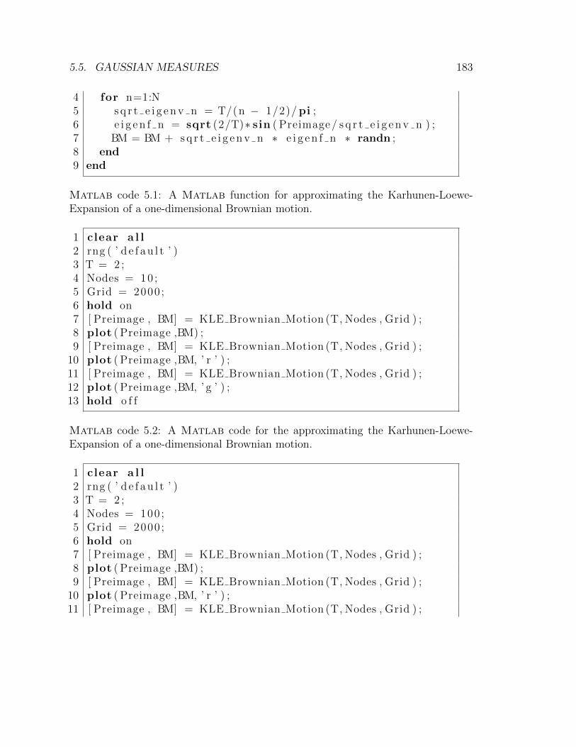
5.5. GAUSSIAN MEASURES 183
4 for n=1:N5 s q r t e i g e n v n = T/(n ´ 1/2)/ pi ;6 e i g e n f n = sqrt (2/T)∗ sin ( Preimage/ s q r t e i g e n v n ) ;7 BM = BM + s q r t e i g e n v n ∗ e i g e n f n ∗ randn ;8 end9 end
Matlab code 5.1: A Matlab function for approximating the Karhunen-Loewe-Expansion of a one-dimensional Brownian motion.
1 clear a l l2 rng ( ’ d e f a u l t ’ )3 T = 2 ;4 Nodes = 10 ;5 Grid = 2000 ;6 hold on7 [ Preimage , BM] = KLE Brownian Motion (T, Nodes , Grid ) ;8 plot ( Preimage ,BM) ;9 [ Preimage , BM] = KLE Brownian Motion (T, Nodes , Grid ) ;
10 plot ( Preimage ,BM, ’ r ’ ) ;11 [ Preimage , BM] = KLE Brownian Motion (T, Nodes , Grid ) ;12 plot ( Preimage ,BM, ’ g ’ ) ;13 hold o f f
Matlab code 5.2: A Matlab code for the approximating the Karhunen-Loewe-Expansion of a one-dimensional Brownian motion.
1 clear a l l2 rng ( ’ d e f a u l t ’ )3 T = 2 ;4 Nodes = 100 ;5 Grid = 2000 ;6 hold on7 [ Preimage , BM] = KLE Brownian Motion (T, Nodes , Grid ) ;8 plot ( Preimage ,BM) ;9 [ Preimage , BM] = KLE Brownian Motion (T, Nodes , Grid ) ;
10 plot ( Preimage ,BM, ’ r ’ ) ;11 [ Preimage , BM] = KLE Brownian Motion (T, Nodes , Grid ) ;

184 CHAPTER 5. RANDOM VARIABLES
12 plot ( Preimage ,BM, ’ g ’ ) ;13 hold o f f
Matlab code 5.3: A Matlab code for approximating the Karhunen-Loewe-Expansion of a one-dimensional Brownian motion.
1 clear a l l2 rng ( ’ d e f a u l t ’ )3 T = 2 ;4 Nodes = 1000 ;5 Grid = 2000 ;6 hold on7 [ Preimage , BM] = KLE Brownian Motion (T, Nodes , Grid ) ;8 plot ( Preimage ,BM) ;9 [ Preimage , BM] = KLE Brownian Motion (T, Nodes , Grid ) ;
10 plot ( Preimage ,BM, ’ r ’ ) ;11 [ Preimage , BM] = KLE Brownian Motion (T, Nodes , Grid ) ;12 plot ( Preimage ,BM, ’ g ’ ) ;13 hold o f f
Matlab code 5.4: A Matlab code for approximating the Karhunen-Loewe-Expansion of a one-dimensional Brownian motion.

5.5. GAUSSIAN MEASURES 185
0 0.2 0.4 0.6 0.8 1 1.2 1.4 1.6 1.8 2−3
−2.5
−2
−1.5
−1
−0.5
0
0.5
1
1.5
2
0 0.2 0.4 0.6 0.8 1 1.2 1.4 1.6 1.8 2−1
−0.5
0
0.5
1
1.5
2
2.5
0 0.2 0.4 0.6 0.8 1 1.2 1.4 1.6 1.8 2−1
−0.5
0
0.5
1
1.5
2
Figure 5.1: Results of calls of the Matlab codes 5.2–5.4.

186 CHAPTER 5. RANDOM VARIABLES

Chapter 6
Stochastic processes with values ininfinite dimensional spaces
6.1 Hilbert space valued stochastic processes
6.1.1 Filtrations
Definition 6.1.1 (Filtration*). Let pΩ,Fq be a measurable space. Then we say thatF is a filtration on pΩ,Fq if and only if it holds
(i) that F is a mapping,
(ii) that DpFq Ď r´8,8s,
(iii) that codomainpFq “ PpΩq, and
(iv) that for all t1, t2 P DpFq with t1 ď t2 it holds that σΩpFt1q “ Ft1 Ď Ft2 Ď F.
Definition 6.1.2 (Filtrations associated to a filtration*). Let pΩ,Fq be a measurablespace and let F be a filtration on pΩ,Fq. Then we denote by F´ P MpDpFq,PpΩqqand F` PMpDpFq,PpΩqq the filtrations on pΩ,Fq which satisfy for all t P DpFq that
F´t “
#
σΩ
`
YsPTXr´8,tq Fs˘
: t ą infpTq
Ft : t “ infpTq(6.1)
and
F`t “
#
XsPTXpt,8s Fs : t ă suppTq
Ft : t “ suppTq. (6.2)
187
188 CHAPTER 6. STOCHASTIC PROCESSES
Lemma 6.1.3 (Properties of the filtrations associated to a filtration*). Let pΩ,Fqbe a measurable space and let F be a filtration on pΩ,Fq. Then
(i) it holds for all t P DpFq that F´t Ď Ft Ď F`t ,
(ii) it holds for all s, t P DpFq with s ă t that Fs Ď F´t Ď Ft, and
(iii) it holds for all s, t P DpFq with s ą t that Ft Ď F`t Ď Fs.
Proof of Lemma 6.1.3*. Items (i)–(iii) are an immediate consequence of Definition 6.1.1,(6.1), and (6.2). The proof of Lemma 6.1.3 is thus completed.
Lemma 6.1.4 (Further properties of the filtrations associated to a filtration*). LetpΩ,Fq be a measurable space, let a P r´8,8s, b P ra,8s, and let pFtqtPra,bs be afiltration on pΩ,Fq. Then it holds for all t P ra, bs that
`
pF´s qsPra,bs˘´
t“ F´t and
`
pF`s qsPra,bs˘`
t“ F`t . (6.3)
Proof of Lemma 6.1.4*. Throughout this proof assume w.l.o.g. that a ă b. Next notethat item (ii) of Lemma 6.1.3 ensures that for all t P pa, bs, r P ra, tq “ ra, bsXr´8, tqit holds that
Fr Ď pYsPra,bsXr´8,tqF´s q. (6.4)
This implies for all t P pa, bs that
pYsPra,bsXr´8,tqFsq Ď pYsPra,bsXr´8,tqF´s q. (6.5)
Hence, we obtain for all t P pa, bs that
F´t “ σΩ
`
YsPra,bsXr´8,tqFs˘
“ σΩ
`
YsPra,bsXr´8,tqF´s˘
“`
pF´s qsPra,bs˘´
t. (6.6)
Next observe that Item (iii) in Lemma 6.1.3 shows that for all t P ra, bq, r P pt, bs “ra, bs X pt,8s it holds that
pXsPra,bsXpt,8sF`s q Ď Fr. (6.7)
This implies for all t P ra, bq that
`
pF`s qsPra,bs˘`
t“ pXsPra,bsXpt,8sF`s q “ pXsPra,bsXpt,8sFsq “ F`t . (6.8)
Combining (6.6) and (6.8) completes the proof of Lemma 6.1.4.
6.1. HILBERT SPACE VALUED STOCHASTIC PROCESSES 189
Definition 6.1.5 (Left-continuity of a filtration*). Let pΩ,Fq be a measurable space.Then we say that F is a left-continuous filtration on pΩ,Fq if and only if F is afiltration on pΩ,Fq which satisfies for all t P DpFq that Ft “ F´t .
Definition 6.1.6 (Right-continuity of a filtration*). Let pΩ,Fq be a measurablespace. Then we say that F is a right-continuous filtration on pΩ,Fq if and only if Fis a filtration on pΩ,Fq which satisfies for all t P DpFq that Ft “ F`t .
Let pΩ,Fq, let T Ď r´8,8s be a set, and let pFtqtPT be a filtration on pΩ,FqThen, in general, it does not hold that for all t P T with t ą infpTq it holds thatF´t “ YsPTXp´8,tqFs because, in general, it does not hold that for all t P T witht ą infpTq it holds that YsPTXp´8,tqFs is a sigma-algebra. This is illustrated in thenext example.
Example 6.1.7. Let pΩ,Fq be the measurable space given by Ω “ N0 “ t0, 1, 2, . . . uand F “ PpΩq, let T Ď R be the set given by T “ r0, 1s, and let Ft Ď PpΩq, t P T,be the sets which satisfy for all n P N0, t P r1´ 12n, 1´ 12pn`1qq that
Ft “ σΩ
`
t0u, t1u, t2u, . . . , tnu(˘
(6.9)
and F1 “ PpΩq. Then
(i) observe
• that for all t P r0, 12q it holds that Ft “ σΩ
`
t0u(˘
,
• that for all t P r12, 3
4q it holds that Ft “ σΩ
`
t0u, t1u(˘
,
• that for all t P r34, 7
8q it holds that Ft “ σΩ
`
t0u, t1u, t2u(˘
,
• . . . ,
(ii) observe that pFtqtPT is a right-continuous filtration on pΩ,Fq,
(iii) observe that pFtqtPT is not a left-continuous filtration on pΩ,Fq,
(iv) observe that for all n P Ω it holds that
tnu P YsPTXp´8,1qFs “ YsPr0,1qFs, (6.10)
(v) observe that
YnPt0,2,4,6,... utnu “ t0, 2, 4, 6, . . . u R YsPTXp´8,1qFs “ YsPr0,1qFs, (6.11)
and
(vi) observe that YsPTXp´8,1qFs “ YsPr0,1qFs is not a sigma-algebra.

190 CHAPTER 6. STOCHASTIC PROCESSES
Class exercise 6.1.8 (*). Let pΩ,Fq be a measurable space, let T Ď r´8,8s be aset, and let pFtqtPT be a filtration on pΩ,Fq.
(i) Is pF´t qtPT a left-continuous filtration on pΩ,Fq?
(ii) Is pF`t qtPT a right-continuous filtration on pΩ,Fq?
Definition 6.1.9 (*). A quadrupel pΩ,F ,P,Fq is called a filtered probability space ifand only if it holds
(i) that pΩ,F ,Pq is a probability space and
(ii) that F is a filtration on pΩ,Fq.
Next we present the notions of a normal filtration (cf., e.g., Definition 2.1.11 in[18]) and of a stochastic basis (cf. Appendix E in [18]).
Definition 6.1.10 (Normal filtration*). Let pΩ,F ,Pq be a probability space. Thenwe say that F is a normal filtration on pΩ,F ,Pq if and only if it holds
(i) that F is a right-continuous filtration on pΩ,Fq and
(ii) that tA P F : PpAq “ 0u Ď pXtPDpFqFtq.
Definition 6.1.11 (Stochastic basis*). A quadrupel pΩ,F ,P,Fq is called a stochasticbasis if and only if it holds
(i) that pΩ,F ,P,Fq is a filtered probability space and
(ii) that F is a normal filtration on pΩ,F ,Pq.
Let a P r´8,8s, b P ra,8s, let pΩ,F ,Pq be a probability space, and let pFtqtPra,bsbe a filtration on pΩ,Fq. Then sometimes the quadrupel pΩ,F ,P, pFtqtPra,bsq is calleda stochastic basis in the literature although pFtqtPra,bs is not necessarily normal.
Proposition 6.1.12 (Construction of a stochastic basis*). Let pΩ,Fq be a measur-able space, let a P r´8,8s, b P ra,8s, let pFtqtPra,bs be a filtration on pΩ,Fq, and letGt Ď PpΩq, t P ra, bs, be the mapping with the property that for all t P ra, bs it holdsthat
Gt “ σΩpFt Y tA P F : PpAq “ 0uq . (6.12)
Then

6.1. HILBERT SPACE VALUED STOCHASTIC PROCESSES 191
(i) it holds that pΩ,F ,P, pG`t qtPra,bsq is a stochastic basis and
(ii) it holds for all normal filtrations pHtqtPra,bs on pΩ,F ,Pq with @ t P ra, bs : Ft ĎHt that @ t P ra, bs : G`t Ď Ht.
Proof of Proposition 6.1.12*. First, observe that (6.12) ensures that for all t P ra, bsit holds that
tA P F : PpAq “ 0u Ď Gt. (6.13)
Item (i) in Lemma 6.1.3 hence ensures that for all t P ra, bs it holds that
tA P F : PpAq “ 0u Ď G`t . (6.14)
Combining this with Lemma 6.1.4 establishes that pG`t qtPra,bs is a normal filtra-tion on pΩ,F ,Pq. This proves (i). Next observe that (6.12) ensures that for allnormal filtrations pHtqtPra,bs on pΩ,F ,Pq with @ t P ra, bs : Ft Ď Ht it holds that@ t P ra, bs : Gt Ď Ht. This implies that for all normal filtrations pHtqtPra,bs on pΩ,F ,Pqwith @ t P ra, bs : Ft Ď Ht it holds that
@ t P ra, bs : G`t Ď H`t “ Ht. (6.15)
This establishes (ii). The proof of Proposition 6.1.12 is thus completed.
6.1.2 Standard Wiener processes
Definition 6.1.13 (*). Let T P r0,8q, let pH, 〈¨, ¨〉H , ¨Hq be a separable R-Hilbertspace, let Q P L1pHq be nonnegative and symmetric, and let pΩ,F ,P, pFtqtPr0,T sq bea filtered probability space. Then we say that W is a Q-standard pΩ,F ,P, pFtqtPr0,T sq-Wiener process if and only if it holds that W PMpr0, T sˆΩ, Hq is an pFtqtPr0,T s/BpHq-adapted stochastic process which satisfies
(i) that PpW0 “ 0q “ 1,
(ii) that there exists a set A P tB P F : PpBq “ 1u such that for all ω P A it holdsthat r0, T s Q t ÞÑ Wtpωq P H is continuous,
(iii) that for all t1, t2 P r0, T s with t1 ď t2 it holds that σΩpWt2 ´Wt1q and Ft1 areP-independent, and
(iv) that for all t1, t2 P r0, T s with t1 ď t2 it holds that pWt2 ´ Wt1qpPqBpHq “N0,Qpt2´t1q.

192 CHAPTER 6. STOCHASTIC PROCESSES
Definition 6.1.14 (*). Let T P r0,8q, let pH, 〈¨, ¨〉H , ¨Hq be an R-Hilbert space,let Q P L1pHq be nonnegative and symmetric, and let pΩ,F ,Pq be a probability space.Then we say that W is a Q-standard P-Wiener process if and only if it holds (thatW P Mpr0, T s ˆ Ω, Hq and that W is a Q-standard pΩ,F ,P, pFWt qtPr0,T sq-Wienerprocess).
Theorem 6.1.15 (*). Let T P r0,8q, let pH, 〈¨, ¨〉H , ¨Hq be an R-Hilbert space, andlet Q P L1pHq be nonnegative and symmetric. Then there exist a probability spacepΩ,F ,Pq and a Q-standard P-Wiener process W : r0, T s ˆ Ω Ñ H.
Theorem 6.1.15 can, e.g., be proved by using a Karhunen-Loeve expansion similaras in the proof of Theorem 5.5.11.
Proposition 6.1.16 (Normalization*). Let T P r0,8q, let pΩ,F ,P, pFtqtPr0,T sq bea filtered probability space, let pH, 〈¨, ¨〉H , ¨Hq be a separable R-Hilbert space, letQ P L1pHq be nonnegative and symmetric, let W : r0, T s ˆ Ω Ñ H be a Q-standardpΩ,F ,P, pFtqtPr0,T sq-Wiener process, and let Gt Ď PpΩq, t P r0, T s, be the mappingwith the property that for all t P r0, T s it holds that
Gt “ σΩpFt Y tA P F : PpAq “ 0uq . (6.16)
Then
(i) it holds that pΩ,F ,P, pG`t qtPr0,T sq is a stochastic basis,
(ii) it holds for all normal filtrations pHtqtPr0,T s on pΩ,F ,Pq with @ t P r0, T s : Ft ĎHt that @ t P r0, T s : G`t Ď Ht, and
(iii) it holds that W is a Q-standard pΩ,F ,P, pG`t qtPr0,T sq-Wiener process.
Proof of Proposition 6.1.16*. First, observe that Item (i) and Item (ii) follow imme-diately from Items (i)–(ii) in Proposition 6.1.12. It thus remains to prove Item (iii).For this note that Definition 6.1.13 ensures that for all t1, t2 P r0, T s with t1 ď t2 itholds that σΩpWt2 ´Wt1q and Ft1 are P-independent. Hence, we obtain that for allt1 P r0, T s, t2 P rt1, T s, A P Ft1 , W P σΩpWt2 ´Wt1q it holds that
PpAXWq “ PpAq ¨ PpWq. (6.17)
This ensures that for all t1 P r0, T s, t2 P rt1, T s, A P Ft1 , B P tS P F : PpSq P t0, 1uu,W P σΩpWt2 ´Wt1q it holds that
P`
pAXBq XW˘
“ P`
pAXWq XB˘
“
#
PpAXWq : PpBq “ 1
0 : PpBq “ 0
“ PpAXBq ¨ PpWq.(6.18)

6.1. HILBERT SPACE VALUED STOCHASTIC PROCESSES 193
Next observe that for all t P r0, T s it holds that
Gt “ σΩ
´
Ft Y σΩ
`
A P F : PpAq “ 0(˘
¯
“ σΩ
´
Ft Y
A P F : PpAq P t0, 1u(
¯
“ σΩ
´!
pAXBq P PpΩq : A P Ft and B P
S P F : PpSq P t0, 1u(
)¯
.
(6.19)
Combining this and the fact that for every t P r0, T s it holds that the set tpA XBq P PpΩq : A P Ft and B P tS P F : PpSq P t0, 1uuu is X-stable with (6.18) andLemma 5.1.10 establishes that for all t1 P r0, T s, t2 P rt1, T s it holds that Gt1 andσΩpWt2 ´Wt1q are P-independent. This implies that for all t1 P r0, T s, t2 P rt1, T s,A P Gt1 , ϕ P CpH,Rq, ψ P CpR,Rq with sup
`
t|ϕpxq| : x P HuYt|ψpxq| : x P Ru˘
ă 8
it holds that
ErϕpWt2 ´Wt1qψp1Aqs “ ErϕpWt2 ´Wt1qs ¨Erψp1Aqs . (6.20)
Hence, we obtain that for all t1 P r0, T q, t2 P pt1, T s, n P N X p1t2´t1,8q, A P G`t1 ,ϕ P CpH,Rq, ψ P CpR,Rq with sup
`
t|ϕpxq| : x P HuYt|ψpxq| : x P Ru˘
ă 8 it holdsthat
E“
ϕpWt2 ´Wt1`1nqψp1Aq‰
“ E“
ϕpWt2 ´Wt1`1nq‰
¨Erψp1Aqs . (6.21)
Lebesgue’s theorem of dominated convergence therefore shows that for all t1 P r0, T q,t2 P pt1, T s, A P G`t1 , ϕ P CpH,Rq, ψ P CpR,Rq with sup
`
t|ϕpxq| : x P Hu Yt|ψpxq| : x P Ru
˘
ă 8 it holds that
ErϕpWt2 ´Wt1qψp1Aqs “ lim supnÑ8
E“
ϕpWt2 ´Wt1`1nqψp1Aq‰
“ lim supnÑ8
`
E“
ϕpWt2 ´Wt1`1nq‰
¨Erψp1Aqs˘
“ ErϕpWt2 ´Wt1qs ¨Erψp1Aqs .
(6.22)
Corollary 5.3.26 hence shows that for all t1 P r0, T q, t2 P pt1, T s, A P G`t1 it holds thatWt2 ´Wt1 and Ω Q ω ÞÑ 1Apωq P R are P-independent. This ensures that for allt1 P r0, T q, t2 P pt1, T s, A P G`t1 , W P BpHq it holds that
P`
AX tWt2 ´Wt1 PWu˘
“ PpAq ¨ PpWt2 ´Wt1 PWq. (6.23)
This shows that for all t1 P r0, T q, t2 P pt1, T s it holds that G`t1 and σΩpWt2 ´Wt1q
are P-independent. This establishes (iii). The proof of Proposition 6.1.16 is thuscompleted.

194 CHAPTER 6. STOCHASTIC PROCESSES
6.1.3 Pseudo inverse
Lemma 6.1.17 (*). Let K P tR,Cu, let pHk, 〈¨, ¨〉Hk , ¨Hkq, k P t1, 2u, be K-Hilbertspaces, and let A P LpH1, H2q. Then
(i) it holds that the mapping A|KernpAqK : KernpAqK Ñ H2 is injective and
(ii) it holds that impAq “ im`
A|KernpAqK˘
.
Proof of Lemma 6.1.17*. First of all, recall that
KernpAqK “
v P H1 :“
@u P KernpAq : 〈v, u〉H1“ 0
‰(
(6.24)
is a K-vector subspace of H1. The mapping A|KernpAqK : KernpAqK Ñ H2 is thus alinear mapping from KernpAqK to H2. It thus holds that A|KernpAqK is injective if andonly if
Kern`
A|KernpAqK˘
“ t0u. (6.25)
Next note that
Kern`
A|KernpAqK˘
“
v P KernpAqK : A|KernpAqKpvq “ 0(
“
v P KernpAqK : Av “ 0(
“
v P KernpAqK : v P KernpAq(
“ KernpAqK XKernpAq “ t0u.
(6.26)
Combining this with (6.25) proves that A|KernpAqK is injective. Moreover, observethat
impAq “ ApH1q “ tAv P H2 : v P H1u
“
A“
PKernpAq,H1 rvs ` PKernpAqK,H1rvs
‰
P H2 : v P H1
(
“
APKernpAqK,H1rvs P H2 : v P H1
(
“
APKernpAqK,H1rvs P H2 : v P KernpAqK
(
“
Av P H2 : v P KernpAqK(
“ im`
A|KernpAqK˘
.
(6.27)
The proof of Lemma 6.1.17 is thus completed.
Lemma 6.1.17 allows us to introduce the following concept.
Definition 6.1.18 (*). Let K P tR,Cu, let pHk, 〈¨, ¨〉Hk , ¨Hkq, k P t1, 2u, be K-Hilbert spaces, and let A P LpH1, H2q. Then we denote by A´1 : impAq Ñ H1 thelinear operator with the property that for all v P impAq it holds that
A´1pvq “ A|´1KernpAqK
pvq (6.28)
and we call A´1 the pseudo inverse of A.

6.1. HILBERT SPACE VALUED STOCHASTIC PROCESSES 195
Class exercise 6.1.19 (*). Let K P tR,Cu, let pHk, 〈¨, ¨〉Hk , ¨Hkq, k P t1, 2u, beK-Hilbert spaces, and let A P LpH1, H2q. What is impA´1q?
The next exercise illustrate the notion of the pseudo inverse in a specific exampleand, in particular, helps us to get more familiar with the concept of the pseudoinverse.
Exercise 6.1.20 (*). Let A : L2pBorelp0,1q; |¨|Rq Ñ R be the linear mapping with theproperty that for all v P L2pBorelp0,1q; |¨|Rq it holds that
Av “
ż 1
0
vpxq dx. (6.29)
Specify DpA´1q, impA´1q, codomainpA´1q, and A´1v, v P DpA´1q, explicity. Showthat your specifications are indeed correct.
In the following proposition we present an important property of the pseudoinverse of a bounded linear operator.
Proposition 6.1.21 (Minimality property of the pseudo inverse). Let K P tR,Cu,let pHk, 〈¨, ¨〉Hk , ¨Hkq, k P t1, 2u, be K-Hilbert spaces, let A P LpH1, H2q, and letv P impAq “ DpA´1q. Then A´1vH1
“ infuPA´1ptvuq uH1and
A´1v(
“
#
w P H1 :
«
Aw “ v and wH1“ inf
uPH1,Au“v
uH1
ff+
“
"
w P A´1ptvuq : wH1
“ infuPA´1ptvuq
uH1
*
“ A´1ptvuq X
“
KernpAqK‰
.
(6.30)
Proof of Proposition 6.1.21. First of all, note that Lemma 6.1.17 and the definitionof the pseudo inverse prove that
A´1v(
“
!
A|´1KernpAqK
pvq)
“
w P KernpAqK : Aw “ v(
““
KernpAqK‰
X A´1ptvuq.
(6.31)Next recall that KernpAq Ď H1 is a closed subspace of H1. Definition 3.4.12 thusshows that for all w P A´1ptvuq “ tu P H1 : Au “ vu it holds that
A|KernpAqK“
PKernpAqK rws‰
“ A“
PKernpAqK rws‰
“ A“
w ´ PKernpAq rws‰
“ Aw “ v.(6.32)

196 CHAPTER 6. STOCHASTIC PROCESSES
The fact that A|KernpAqK is injective (see Lemma 6.1.17) hence proves that for allw P A´1ptvuq “ tu P H1 : Au “ vu it holds that
PKernpAqK rws “ A´1v. (6.33)
This implies that for all w P A´1ptvuq “ tu P H1 : Au “ vu it holds that
wH1“›
›PKernpAq rws ` PKernpAqK rws›
›
H1
“
b
›
›PKernpAq rws›
›
2
H1`›
›PKernpAqK rws›
›
2
H1
“
b
›
›PKernpAq rws›
›
2
H1` A´1pvq2H1
ě›
›A´1pvq
›
›
2
H1.
(6.34)
This and the fact that A´1pvq P A´1ptvuq prove that
infuPA´1ptvuq
uH1“›
›A´1pvq
›
›
H1. (6.35)
This, (6.34), and (6.31) imply that"
w P A´1ptvuq : wH1
“ infuPA´1ptvuq
uH1
*
“
!
w P A´1ptvuq : wH1
“›
›A´1pvq
›
›
H1
)
“
"
w P A´1ptvuq :
b
›
›PKernpAq rws›
›
2
H1` A´1pvq2H1
“›
›A´1pvq
›
›
H1
*
“
!
w P A´1ptvuq :
›
›PKernpAq rws›
›
2
H1“ 0
)
“
w P A´1ptvuq : PKernpAq rws “ 0
(
“ A´1ptvuq X
“
KernpAqK‰
“
A´1pvq
(
.
(6.36)
This, (6.31), and (6.35) complete the proof of Proposition 6.1.21.
The pseudo inverse allows us to define a Hilbert space structure on the imageof a bounded linear operator on Hilbert spaces. This is the subject of the nextproposition.
Proposition 6.1.22 (Image Hilbert space*). LetK P tR,Cu, let pHk, 〈¨, ¨〉Hk , ¨Hkq,k P t1, 2u, be K-Hilbert spaces, and let A P LpH1, H2q. Then it holds that
`
impAq,⟨A´1p¨q, A´1p¨q
⟩H1,›
›A´1p¨q›
›
H1
˘
(6.37)
is an K-Hilbert space.

6.2. SPACE-TIME WHITE NOISE AND BROWNIAN SHEET 197
Proof of Proposition 6.1.22*. First of all, note that the fact that A´1 : impAq Ñ H1
is a linear operator implies that
`
impAq,⟨A´1p¨q, A´1p¨q
⟩H1,›
›A´1p¨q›
›
H1
˘
(6.38)
is aK-inner product space. It thus remains to prove that pimpAq, A´1p¨qH1q is com-
plete. To see this let pvnqnPN Ď impAq be a Cauchy sequence in pimpAq, A´1p¨qH1q.
Hence, we obtain that A´1pvnq P KernpAqK, n P N, is a Cauchy sequence inpKernpAqK, ¨H1
q. Completeness of pKernpAqK, ¨H1q hence proves that there ex-
ists a vector w P KernpAqK such that
lim supnÑ8
›
›w ´ A´1pvnq›
›
H1“ 0. (6.39)
This proves that Aw P impAq satisfies limnÑ8 A´1pAw ´ vnqH1
“ 0. The proof ofProposition 6.1.22 is thus completed.
6.2 Space-time white noise and Brownian sheet
6.2.1 Derivative of a Brownian sheet
Definition 6.2.1 (Law of white noise). Let d,m P N and let D Ď Rd be an openset. Then we say that µ is the law of white noise on L2pD;Rmq if and only ifµ P M
`
BpDpD,Rmq1q, r0,8s˘
is a Gaussian measure which satisfies for all v, w P
DpD,Rmq that
ż
DpD,Rmq1φpvq ` φpvqφpwqµpdφq “ 〈v, w〉L2pBorelD;Rmq . (6.40)
Definition 6.2.2 (White noise). Let pΩ,F ,Pq be a probability space, let d,m P
N, and let D Ď Rd be an open set. Then we say that X is a P-white noise onL2pD;Rmq if and only if (it holds that X PMpF ,BpDpD,Rmq1qq and it holds thatXpPqBpDpD,Rmq1q is the law of white noise on L2pD,Rmqq.
Remark 6.2.3 (Space-time white noise). Let pΩ,F ,Pq be a probability space, letd P t2, 3, . . . u, m P N, and let D Ď Rd be an open set. Then in the literature X issometimes referred to as a space-time white noise on L2pD;Rmq with respect to P ifand only if X is a P-space-time white noise on L2pD;Rmq.

198 CHAPTER 6. STOCHASTIC PROCESSES
Theorem 6.2.4 (“Coordinate free” property of white noise). Let pΩ,F ,Pq be aprobability space, let d,m P N, let D Ď Rd be an open set, and let X : Ω Ñ DpD,Rmq1
be a F/BpDpD,Rmq1q-measurable mapping. Then X is a P-white noise on L2pD;Rmq
if and only if for all orthonormal basis H Ď L2pD;Rmq of L2pD;Rmq there existsa family ξh PMpF ,BpRqq, h P H, of i.i.d. standard normal random variables suchthat
X “ÿ
hPH
ξh h. (6.41)
Theorem 6.2.5 (Distributional derivative of Brownian motion). Let m P N, letpΩ,F ,Pq be a probability space, let W : r0, T s ˆ Ω Ñ Rm be a standard Brownianmotion with continuous sample paths, and let X : Ω Ñ Dpp0, T q;Rmq1 be the functionwhich satisfies for all ω P Ω, ϕ P Dpp0, T q,Rmq that
`
Xpωq˘
pϕq “ ´
ż T
0
〈ϕ1ptq,Wtpωq〉Rm dt “`
BWp¨qpωq˘
pϕq. (6.42)
Then X is a P-white noise on L2pp0, T q;Rmq.
6.3 Stochastic integration with respect to infinite
dimensional Wiener processes
The following presentations are similiar to the presentations in Section 2.3 in Prevot& Rockner [18] and in Chapter 3 in the lecture notes of the course Numerical Analysisof Stochastic Ordinary Differential Equations.
6.3.1 Lenglart’s inequality
Definition 6.3.1 (Random time). Let T Ď pRYt´8,8uq be a set, let pΩ,F ,Pq bea probability space, and let τ : Ω Ñ T be an F/BpTq-measurable mapping. Then τis called a random time.
Observe, in the setting of Definition 6.3.1, that for every t P T it holds thattτ ď tu P F .
Definition 6.3.2 (Stopping time). Let T Ď pR Y t´8,8uq be a set, let pΩ,F ,Pqbe a probability space with a filtration pFtqtPT, and let τ : Ω Ñ T be a mappingwith the property that for all t P T it holds that tτ ď tu P Ft. Then τ is called anpFtqtPT-stopping time.
6.3. STOCHASTIC INTEGRATION 199
A stopping time on a filtered probability space also induces a sigma-algebra. Thisis the subject of the next definition.
Definition 6.3.3. Let T Ď pR Y t´8,8uq be a set, let pΩ,F ,Pq be a probabilityspace with a filtration pFtqtPT, and let τ : Ω Ñ T be an pFtqtPT-stopping time. Thenwe denote by Fτ the set given by
Fτ “ tA P pYtPTFtq : p@ t P T : AX tτ ď tu P Ftqu (6.43)
and we call Fτ the sigma-algebra at the stopping time τ .
Exercise 6.3.4. Let T Ď pRYt´8,8uq be a set, let pΩ,F ,Pq be a probability spacewith a filtration pFtqtPT, and let τ, ρ : Ω Ñ T be pFtqtPT-stopping times. Prove thenthat mintτ, ρu is an pFtqtPT-stopping time.
In (6.46) in the following result, Proposition 6.3.5, we prove a powerful inequalitywhich is known as Lenglart inequality in the literature. Proposition 6.3.5 and itsproof are extensions of Problem 1.4.15, Remark 1.4.17 and Solution 4.15 in Section1.6 in [12].
Proposition 6.3.5 (Lenglart inequality). Let pΩ,F ,Pq be a probability space witha filtration pFtqtPr0,8q, let X, Y : r0,8qˆΩ Ñ r0,8q be pFtqtPr0,8q/Bpr0,8qq-adaptedstochastic processes with continuous sample paths such that for all bounded pFtqtPr0,8q-stopping times τ : Ω Ñ r0,8q it holds that E
“
Xτ
‰
ď E“
suptPr0,τ s Yt‰
. Then for allε, δ P p0,8q and all pFtqtPr0,8q-stopping times τ : Ω Ñ r0,8q it holds that
P`
suptPr0,τ sXt ě ε˘
ď 1εE“
suptPr0,τ s Yt‰
, (6.44)
P`
suptPr0,τ sXt ě ε, suptPr0,τ s Yt ă δ˘
ď 1εE“
min
δ, suptPr0,τ s Yt(‰
, (6.45)
P`
suptPr0,τ sXt ě ε˘
ď 1εE“
min
δ, suptPr0,τ s Yt(‰
` P`
suptPr0,τ s Yt ě δ˘
, (6.46)
E“
min
ε, suptPr0,τ sXt
(‰
ď
”
2?ε` ε?
δ
ı
ˇ
ˇE“
min
δ, suptPr0,τ s Yt(‰ˇ
ˇ
12, (6.47)
E“
min
1, suptPr0,τ sXt
(‰
ď 3ˇ
ˇE“
min
1, suptPr0,τ s Yt(‰ˇ
ˇ
12. (6.48)
Proof of Proposition 6.3.5. Throughout this proof let ρXε : Ω Ñ r0,8s, ε P r0,8q,and ρYε : Ω Ñ r0,8s, ε P r0,8q, be the mappings with the property that for allε P r0,8q it holds that
ρXε “ inf`
t P r0,8q : Xt ě ε(
Y t8u˘
, (6.49)

200 CHAPTER 6. STOCHASTIC PROCESSES
ρYε “ inf`
t P r0,8q : supsPr0,ts Ys ě ε(
Y t8u˘
. (6.50)
Then observe that for all ε P r0,8q, n P N and all pFtqtPr0,8q-stopping times τ : Ω Ñr0,8q it holds that
εP`
suptPr0,mintτ,nusXt ě ε˘
“ εP´
D t P r0,mintτ, nus : Xt ě ε¯
“ εP´!
D t P r0,mintτ, nus : Xt ě ε)
X
!
ρXε ď mintτ, nu)¯
“ εP´!
D t P r0,mintτ, nus : Xt ě ε)
X
!
ρXε ď mintτ, nu)
X
!
Xmintτ,n,ρXε uě ε
)¯
ď εP´
Xmintτ,n,ρXε uě ε
¯
“ E
”
ε1tXmintτ,n,ρXε u
ěεu
ı
ď E
”
Xmintτ,n,ρXε u1tX
mintτ,n,ρXε uěεu
ı
ď E“
Xmintτ,n,ρXε u
‰
.
(6.51)
Combining this with the fact for all ε P r0,8q, n P N and all pFtqtPr0,8q-stoppingtimes τ : Ω Ñ r0,8q it holds that mintτ, n, ρXε u is a bounded pFtqtPr0,8q-stopping time(see Exercise 6.3.4) ensures that for all ε P r0,8q, n P N and all pFtqtPr0,8q-stoppingtimes τ : Ω Ñ r0,8q it holds that
εP`
suptPr0,mintτ,nusXt ě ε˘
ď E“
Xmintτ,n,ρXε u
‰
ď E“
suptPr0,mintτ,n,ρXε usYt‰
ď E“
suptPr0,τ s Yt‰
.(6.52)
Hence, we obtain that for all ε P r0,8q and all pFtqtPr0,8q-stopping times τ : Ω Ñ
r0,8q it holds that
εP`
suptPr0,τ sXt ě ε˘
“ εP`
YnPN
suptPr0,mintτ,nusXt ě ε(˘
“ ε limnÑ8
P`
suptPr0,mintτ,nusXt ě ε˘
ď E“
suptPr0,τ s Yt‰
.(6.53)
This proves (6.44). In the next step we observe that (6.44) ensures that for allε, δ P p0,8q and all pFtqtPr0,8q-stopping times τ : Ω Ñ p0,8q it holds that
P`
suptPr0,τ sXt ě ε, suptPr0,τ s Yt ă δ˘
“ P`
suptPr0,τ sXt ě ε, ρYδ ą τ, suptPr0,τ s Yt ă δ˘
“ P´
suptPr0,mintτ,ρYδ usXt ě ε, ρYδ ą τ, suptPr0,τ s Yt ă δ
¯
ď P´
suptPr0,mintτ,ρYδ usXt ě ε
¯
ď 1εE
”
suptPr0,mintτ,ρYδ usYt
ı
“ 1εE
”
min
δ, suptPr0,mintτ,ρYδ usYt(
ı
ď 1εE“
min
δ, suptPr0,τ s Yt(‰
.
(6.54)
6.3. STOCHASTIC INTEGRATION 201
This proves (6.45). Furthermore, we observe that (6.45) shows that for all ε, δ Pp0,8q and all pFtqtPr0,8q-stopping times τ : Ω Ñ p0,8q it holds that
P`
suptPr0,τ sXt ě ε˘
ď P`
suptPr0,τ sXt ě ε, suptPr0,τ s Yt ă δ˘
` P`
suptPr0,τ s Yt ě δ˘
ď 1εE“
min
δ, suptPr0,τ s Yt(‰
` P`
suptPr0,τ s Yt ě δ˘
.
(6.55)
This proves (6.46). Next we note that (6.46) and the Markov inequality show thatfor all r, δ P p0,8q and all pFtqtPr0,8q-stopping times τ : Ω Ñ p0,8q it holds that
P`
suptPr0,τ sXt ě r˘
ď 1rE“
min
δ, suptPr0,τ s Yt(‰
` P`
min
δ, suptPr0,τ s Yt(
ě δ˘
ď“
1r` 1
δ
‰
E“
min
δ, suptPr0,τ s Yt(‰
.
(6.56)
This implies that for all ε, δ, r P p0,8q and all pFtqtPr0,8q-stopping times τ : Ω Ñ
p0,8q it holds that
E“
min
ε, suptPr0,τ sXt
(‰
“ E
”
min
ε, suptPr0,τ sXt
(
1tsuptPr0,τsXtăru
ı
`E
”
min
ε, suptPr0,τ sXt
(
1tsuptPr0,τsXtěru
ı
ď mintε, ru ` εP`
suptPr0,τ sXt ě r˘
ď mintε, ru ` ε“
1r` 1
δ
‰
E“
min
δ, suptPr0,τ s Yt(‰
ď r ` ε“
1r` 1
δ
‰
E“
min
δ, suptPr0,τ s Yt(‰
.
(6.57)
Hence, we obtain that for all ε, δ P p0,8q and all pFtqtPr0,8q-stopping times τ : Ω Ñp0,8q it holds that
E“
min
ε, suptPr0,τ sXt
(‰
ď infrPp0,8q
`
r ` εrE“
min
δ, suptPr0,τ s Yt(‰
` εδE“
min
δ, suptPr0,τ s Yt(‰˘
ďˇ
ˇεE“
min
δ, suptPr0,τ s Yt(‰ˇ
ˇ
12
`?εˇ
ˇE“
min
δ, suptPr0,τ s Yt(‰ˇ
ˇ
12` ε
δE“
min
δ, suptPr0,τ s Yt(‰
.
(6.58)
This proves (6.47). Moreover, we note that (6.48) is an immediate consequence of(6.47). The proof of Proposition 6.3.5 is thus completed.

202 CHAPTER 6. STOCHASTIC PROCESSES
Exercise 6.3.6 (Characterization of convergence in probability). Let pΩ,F ,Pq bea probability space, let pE, dEq be a metric space, and let Xn : Ω Ñ E, n P N0, beF/pE, dEq-strongly measurable mappings. Then the following three statements areequivalent:
(i) For all c P p0,8q it holds that
limnÑ8
E“
mintc, dEpX0, Xnqu‰
“ 0. (6.59)
(ii) There exists a c P p0,8q such that
limnÑ8
E“
mintc, dEpX0, Xnqu‰
“ 0. (6.60)
(iii) For all ε P p0,8q it holds that
limnÑ8
PpdEpX0, Xnq ą εq “ 0. (6.61)
6.3.2 Modifications and indistinguishability
This material is an extended version from Barth et al. 2014. Next we address twonotions that somehow describe when two stochastic processes are “equal up to setsof measure zero”.
Definition 6.3.7 (Modifications). Let pΩ,F ,Pq be a probability space, let pS,Sq bea measurable space, let T Ď R be a set, and let X, Y : T ˆ Ω Ñ S be stochasticprocesses such that for every t P T it holds that there exists an event A P F withPpAq “ 1 and
A Ď tXt “ Ytu. (6.62)
Then X and Y are called modifications of each other (i.e., X is called a modificationof Y and Y is called a modification of X).
Exercise 6.3.8. Prove or disprove the following statement: For all measurable spacespΩ,Fq it holds that tpω, ωq P Ω2 : ω P Ωu P F b F .
Exercise 6.3.9. Specify explicitly measurable spaces pΩ,Fq and pS,Sq and F/S-measurable mappings X, Y : Ω Ñ S such that tX “ Y u “ tω P Ω: Xpωq “ Y pωqu RF . Prove that your result is correct.

6.3. STOCHASTIC INTEGRATION 203
Definition 6.3.10 (Indistinguishablility). Let pΩ,F ,Pq be a probability space, letpS,Sq be a measurable space, let T Ď R be a set, and let X, Y : T ˆ Ω Ñ S bestochastic processes with the property that there exists an event A P F with PpAq “ 1and
A Ď pXtPTtXt “ Ytuq . (6.63)
Then X and Y are called indistinguishable from each other (i.e., X is called indis-tinguishable from Y and Y is called indistinguishable from X).
Let us illustrate Definitions 6.3.7 and 6.3.10 through a simple example (see, e.g.,Kuhn [15]).
Example 6.3.11. Let pΩ,F ,Pq be a probability space, let pFtqtPr0,1s be the filtrationon pΩ,Fq with the property that for all t P r0, 1s it holds that Ft “ F , let τ : Ω Ñ r0, 1sbe an F/Bpr0, 1sq-measurable mapping such that τpPq “ Borelr0,1s, let X, Y : r0, 1s ˆΩ Ñ R be the functions with the property that for all ω P Ω, t P r0, 1s it holds that
Xtpωq “ 0 and Ytpωq “
#
1 : t “ τpωq
0 : t ‰ τpωq. (6.64)
Then
(i) it holds that X, Y are pFtqtPr0,T s-predictable stochastic processes (indeed, letY n : r0, T s ˆ Ω Ñ R, n P N, be the mappings with the property that for alln P N, t P r0, T s it holds that Y n
t pωq “ 1pτpωq´1n,τpωqsptq, observe that forall n P N it holds that Y n is pFtqtPr0,T s-predictable and note that @ pt, ωq Pr0, T s ˆ Ω: limnÑ8 Y
nt pωq “ Ytpωq),
(ii) it holds that τ is an pFtqtPr0,T s-stopping time,
(iii) it holds for all ω P Ω that Xτpωqpωq “ 0 ‰ 1 “ Yτpωqpωq,
(iv) it holds that!
ω P Ω:`
@ t P r0, T s : Xtpωq “ Ytpωq˘
)
“
!
ω P Ω:`
@ t P r0, T s : Ytpωq “ 0˘
)
“ H,(6.65)
(v) it holds for all t P r0, T s that
PpXt “ Ytq “ PpYt “ 0q “ Ppτ ‰ tq “ 1, (6.66)
(vi) and it holds that X and Y are modification of each other but X and Y are notindistinguishable from of each other.

204 CHAPTER 6. STOCHASTIC PROCESSES
6.3.3 Predictability
Definition 6.3.12 (Predictable sigma-algebra*). Let T P r0,8q and let pΩ,Fq be ameasurable space with a filtration pFtqtPr0,T s. Then we denote by Pred
`
pFtqtPr0,T s˘
thesigma-algebra given by
Pred`
pFtqtPr0,T s˘
“
σr0,T sˆΩ
´
tps, ts ˆ A : A P Fs and s, t P r0, T s with s ă tu Y tt0u ˆ A : A P F0u
¯
(6.67)
and we call Pred`
pFtqtPr0,T s˘
the predictable sigma-algebra of pFtqtPr0,T s.
Note, in the setting of Definition 6.3.12, that the definition of the sigma-algebraPred
`
pFtqtPr0,T s˘
depends on the filtration pFtqtPr0,T s.
Definition 6.3.13 (Predictability*). Let T P r0,8q, let pS,Sq be a measurable space,and let pΩ,Fq be a measurable space with a filtration pFtqtPr0,T s. Then we say that Xis an pFtqtPr0,T s/S-predictable process (we say that X is an pFtqtPr0,T s/S-predictablestochastic process, we say X is a predictable process, we say that X is a predictablestochastic process) if and only if X P Mpr0, T s ˆ Ω, Sq is an Pred
`
pFtqtPr0,T s˘
/S-measurable mapping.
Observe that for every T P p0,8q and every measurable space pΩ,Fq with afiltration pFtqtPr0,T s it holds that
PredppFtqtPr0,T sq Ď σr0,T sˆΩ
`
B ˆ A : B P Bpr0, T sq and A P FT˘
“ Bpr0, T sq b FT .(6.68)
This is fact is used in the next definition.
Definition 6.3.14 (Product measure on the predictable sigma-algebra*). Let T Pp0,8q and let pΩ,F ,Pq be a probability space with a filtration pFtqtPr0,T s. Then wedenote by
PP,pFtqtPr0,T s : PredppFtqtPr0,T sq Ñ r0,8s (6.69)
the measure given by
PP,pFtqtPr0,T s “ pBorelr0,T sbPq|PredppFtqtPr0,T sq. (6.70)
Let T P p0,8q and let pΩ,F ,Pq be a probability space with a filtration pFtqtPr0,T s.Then we note that for all t1, t2 P r0, T s, A P Ft1 with t1 ă t2 it holds that
PP,pFtqtPr0,T sppt1, t2s ˆ Aq “ pt2 ´ t1q ¨ PpAq. (6.71)
6.3. STOCHASTIC INTEGRATION 205
Class exercise 6.3.15 (Measurability of sample paths?*). Let T P p0,8q, let pS,Sqbe a measurable space with a filtration pFtqtPr0,T s, and let X : r0, T s ˆ Ω Ñ S be anpFtqtPr0,T s/S-predictable stochastic process. Is it then true that for every ω P Ω itholds that
r0, T s Q t ÞÑ Xtpωq P S (6.72)
is a Bpr0, T sq/S-measurable mapping?
6.3.4 Construction of the stochastic integral
In the next step we introduce the notion of an elementary process. For this we recallthe notion of a simple function; see Definition 2.3.1 above.
Definition 6.3.16 (Elementary process). Let T P r0,8q, let pH, 〈¨, ¨〉H , ¨Hq andpU, 〈¨, ¨〉U , ¨Uq be R-Hilbert spaces, let pΩ,Fq be a measurable space with a filtrationpFtqtPr0,T s, and let X : r0, T s ˆ Ω Ñ LpU,Hq be a mapping with the property thatthere exist n P N, 0 ď t1 ă . . . ă tn ď T and for every k P t1, . . . , n ´ 1u anFtk/BpLpU,Hqq-simple function Yk : Ω Ñ LpU,Hq such that for all t P r0, T s it holdsthat
Xt “
n´1ÿ
k“1
Yk ¨ 1ptk,tk`1sptq . (6.73)
Then X is called pFtqtPr0,T s-elementary (or just elementary).
Elementary processes in the sense of Definition 6.3.16 are predictable in the senseof Definition 6.3.13. Let pU, 〈¨, ¨〉U , ¨Uq be an R-Hilbert space, let T P r0,8q,let pΩ,F ,Pq be a probability space, let Q P L1pUq be nonnegative and symmetric,and let W : r0, T s ˆ Ω Ñ U be a Q-standard P-Wiener process. In the stochasticintegration theory with respect to the possibly infinite dimensional Q-standard P-Wiener process W the Hilbert space
´
Q12pUq,
⟨Q´
12p¨q, Q´
12p¨q⟩U,›
›Q´12p¨q›
›
2
U
¯
(6.74)
plays an important role. Recall that Q12 is defined according to Theorem 3.5.15and Q´12 is the pseudo inverse of Q12 (see Definition 6.1.18 above). According toProposition 6.1.22 the triple (6.74) is indeed anR-Hilbert space. Lemma 6.3.20 belowillustrate the appearence of the Hilbert space in (6.74) in the stochastic integrationtheory. Before we present Lemma 6.3.20, we note the following exercise and itspreceding remark.

206 CHAPTER 6. STOCHASTIC PROCESSES
Exercise 6.3.17 (Embedding of LpU,Hq intoHSpQ12pUq, Hq*). Let pH, 〈¨, ¨〉H , ¨Hqand pU, 〈¨, ¨〉U , ¨Uq be R-Hilbert spaces, let Q P L1pUq be nonnegative and symmet-ric, and let A P LpU,Hq. Prove that A|Q12pUq P HSpQ
12pUq, Hq and
›
›A|Q12pUq
›
›
HSpQ12pUq,Hq“›
›AQ12›
›
HSpU,Hqď ALpU,Hq
›
›Q12›
›
HSpUqă 8. (6.75)
Remark 6.3.18 (Embedding of LpU,Hq intoHSpQ12pUq, Hq*). Let pH, 〈¨, ¨〉H , ¨Hqand pU, 〈¨, ¨〉U , ¨Uq be R-Hilbert spaces, let Q P L1pUq be nonnegative and symmet-ric, and let A P LpU,Hq. Then we often simply write A as an abbreviation forA|Q12pUq.
Lemma 6.3.19. Let pU, 〈¨, ¨〉U , ¨Uq be an R-Hilbert space and let Q P L1pUq. ThenQ is a diagonal linear operator if and only if Q is symmetric.
We are now ready to present Lemma 6.3.20, which illustrates the appearence ofthe Hilbert space in (6.74) in the stochastic integration theory.
Lemma 6.3.20 (Baby version of Ito’s isometry*). Let T P r0,8q, s P r0, T s, t Prs, T s, let pΩ,F ,P, pFtqtPr0,T q be a stochastic basis, let pU, 〈¨, ¨〉U , ¨Uq be a separableR-Hilbert space, let A : Ω Ñ LpU,Hq be an Fs/BpLpU,Hqq-simple function, let Q PL1pUq be nonnegative and symmetric, and let W : r0, T s ˆ Ω Ñ U be a Q-standardpΩ,F ,P, pFtqtPr0,T sq-Wiener process. Then
E“
A pWt ´Wsq2H
‰
“ E
”
A2HSpQ12pUq,Hq
ı
pt´ sq . (6.76)
Proof of Lemma 6.3.20*. Throughout this proof let B Ď U be an orthonormal basisof U and let λ : BÑ r0,8q be a globally bounded function such that for all u P U itholds that
Qu “ÿ
bPB
λb 〈b, u〉U b. (6.77)
Next note that the fact that B Ď U is an orthonormal basis of U and the continuity

6.3. STOCHASTIC INTEGRATION 207
of A imply that
E“
A pWt ´Wsq2H
‰
“ E
»
–
›
›
›
›
›
A
˜
ÿ
bPB
〈b,Wt ´Ws〉U b
¸›
›
›
›
›
2
H
fi
fl
“ E
»
–
›
›
›
›
›
ÿ
bPB
〈b,Wt ´Ws〉U Ab
›
›
›
›
›
2
H
fi
fl
“ E
«
ÿ
b1,b2PB
〈b1,Wt ´Ws〉U 〈b2,Wt ´Ws〉U 〈Ab1, Ab2〉H
ff
“ÿ
b1,b2PB
Er〈b1,Wt ´Ws〉U 〈b2,Wt ´Ws〉U 〈Ab1, Ab2〉Hs .
(6.78)
Independency and the definition of a Q-standard pΩ,F ,P, pFtqtPr0,T sq-Wiener processhence assure that
E“
A pWt ´Wsq2H
‰
“ÿ
b1,b2PB
Er〈b1,Wt ´Ws〉U 〈b2,Wt ´Ws〉U sEr〈Ab1, Ab2〉Hs
“ÿ
bPB
E“
|〈b,Wt ´Ws〉U |2‰
E“
Ab2H‰
“ pt´ sqÿ
bPB
〈b,Qb〉U E“
Ab2H‰
“ pt´ sqÿ
bPλ´1pp0,8qq
〈b,Qb〉Ulooomooon
“λb
E“
Ab2H‰
.
(6.79)
This proves that
E“
A pWt ´Wsq2H
‰
“ pt´ sqE
»
–
ÿ
bPλ´1pp0,8qq
›
›
›Aa
λb b›
›
›
2
H
fi
fl
“ pt´ sqE
»
–
ÿ
bPλ´1pp0,8qq
›
›AQ12b›
›
2
H
fi
fl .
(6.80)
Next we observe that the set
Q12pbq P im
`
Q12˘
: b P λ´1pp0,8qq
(
(6.81)
is an orthonormal basis of the R-Hilbert space´
Q12pUq,
⟨Q´
12p¨q, Q´
12p¨q⟩U,›
›Q´12p¨q›
›
2
U
¯
. (6.82)

208 CHAPTER 6. STOCHASTIC PROCESSES
Combining this with (6.80) completes the proof of Lemma 6.3.20.
Lemma 6.3.21 (Ito’s isometry in infinite dimension for elementary processes). Letn P t2, 3, . . . u, T P r0,8q, 0 ď t1 ă ¨ ¨ ¨ ă tn “ T , let pΩ,F ,P, pFtqtPr0,T q bea stochastic basis, let pH, 〈¨, ¨〉H , ¨Hq and pU, 〈¨, ¨〉U , ¨Uq be separable R-Hilbertspaces, for every k P t1, 2, . . . , n ´ 1u let Yk : Ω Ñ LpU,Hq be an Ftk/BpLpU,Hqq-simple function, let Q P L1pUq be nonnegative and symmetric, and let W : r0, T s ˆΩ Ñ U be a Q-standard pΩ,F ,P, pFtqtPr0,T sq-Wiener process. Then
E
»
–
›
›
›
›
›
n´1ÿ
k“1
Yk`
Wtk`1´Wtk
˘
›
›
›
›
›
2
H
fi
fl “ E
«
n´1ÿ
k“1
Yk2HSpQ12pUq,Hq ptk`1 ´ tkq
ff
“
ż T
0
E
»
–
›
›
›
›
›
n´1ÿ
k“1
Yk 1ptk,tk`1spsq
›
›
›
›
›
2
HSpQ12pUq,Hq
fi
fl ds.
(6.83)
Proof of Lemma 6.3.21. Note that
E
»
–
›
›
›
›
›
n´1ÿ
k“1
Yk`
Wtk`1´Wtk
˘
›
›
›
›
›
2
H
fi
fl
“
n´1ÿ
k,l“1
E“⟨Yk
`
Wtk`1´Wtk
˘
, Yl`
Wtl`1´Wtl
˘⟩H
‰
“ 2ÿ
k,lPt1,...,n´1ukăl
E“⟨rYls
˚Yk`
Wtk`1´Wtk
˘
,Wtl`1´Wtl
⟩U
‰
`
n´1ÿ
k“1
E
”
›
›Yk`
Wtk`1´Wtk
˘›
›
2
H
ı
.
(6.84)
Independency and Lemma 6.3.20 hence imply that for all orthonormal bases B Ď U

6.3. STOCHASTIC INTEGRATION 209
of U it holds that
E
»
–
›
›
›
›
›
n´1ÿ
k“1
Yk`
Wtk`1´Wtk
˘
›
›
›
›
›
2
H
fi
fl
“ 2ÿ
k,lPt1,...,n´1ukăl
E
«
ÿ
bPB
⟨b, rYls
˚Yk`
Wtk`1´Wtk
˘⟩U
⟨b,Wtl`1
´Wtl
⟩U
ff
`
n´1ÿ
k“1
E
”
Yk2HSpQ12pUq,Hq
ı
ptk`1 ´ tkq
“ 2ÿ
k,lPt1,...,n´1ukăl
ÿ
bPB
E“⟨b, rYls
˚Yk`
Wtk`1´Wtk
˘⟩U
‰
E“⟨b,Wtl`1
´Wtl
⟩U
‰
`
n´1ÿ
k“1
E
”
Yk2HSpQ12pUq,Hq
ı
ptk`1 ´ tkq “n´1ÿ
k“1
E
”
Yk2HSpQ12pUq,Hq
ı
ptk`1 ´ tkq .
(6.85)
The proof of Lemma 6.3.21 is thus completed.
The random variableřn´1k“1 Yk
`
Wtk`1´Wtk
˘
in (6.83) will be the stochastic in-
tegral of the elementary stochastic processřn´1k“1 Yk 1ptk,tk`1s in (6.83). Our aim is to
integrate more general stochastic processes. To do so the following lemma is crucial.
Lemma 6.3.22 (Density). Let T P r0,8q, let pΩ,F ,P, pFtqtPr0,T sq be a stochasticbasis, let pH, 〈¨, ¨〉H , ¨Hq and pU, 〈¨, ¨〉U , ¨Uq be R-Hilbert spaces, let Q P L1pUqbe nonnegative and symmetric, and let X P L0
`
PP,pFtqtPr0,T s ; ¨HSpQ12pUq,Hq
˘
satisfy
that it holds P-a.s. thatşT
0Xs
2HSpQ12pUq,Hq
ds ă 8. Then there exists a sequence
Xn : r0, T s ˆΩ Ñ LpU,Hq, n P N, of pFtqtPr0,T s-elementary stochastic processes suchthat for all ε P p0,8q it holds that
limnÑ8
Pˆż T
0
Xs ´Xns
2HSpQ12pUq,Hqq ds ě ε
˙
“ 0. (6.86)
Lemma 6.3.22 follows, e.g., from Proposition 2.3.8 in Prevot & Rockner [18].In the next result, Theorem 6.3.23, the existence and uniqueness of the stochasticintegral is established (cf., e.g., Proposition 2.26 in Karatzas & Shreve [12]).

210 CHAPTER 6. STOCHASTIC PROCESSES
Theorem 6.3.23 (Stochastic integral*). Let pH, 〈¨, ¨〉H , ¨Hq and pU, 〈¨, ¨〉U , ¨Uqbe separable R-Hilbert spaces, let T P p0,8q, let Q P L1pUq be nonnegative and sym-metric, let pΩ,F ,P, pFtqtPr0,T sq be a stochastic basis, and let W : r0, T s ˆ Ω Ñ U bea Q-standard pΩ,F ,P, pFtqtPr0,T sq-Wiener process. Then there exists a unique lin-
ear mapping I :
X P L0`
PP,pFtqtPr0,T s ; ¨HSpQ12pUq,Hq
˘
: P`
∫T0 Xs2HSpQ12pUq,Hq
ds ă
8˘
“ 1(
Ñ L0pP; ¨Hq which satisfies
(i) that for all Xn P DpIq, n P N, with lim supnÑ8E“
mint1,şT
0Xn
s 2HSpQ12pUq,Hq
dsu‰
“ 0 it holds that lim supnÑ8E“
mint1, IpXnqHu‰
“ 0 (continuity) and
(ii) that for all s P r0, T s, t P ps, T s and all Fs/BpLpU,Hqq-simple X : Ω Ñ LpU,Hqit holds that
Ip1ps,tsXq “ rX pWt ´WsqsP,BpHq (6.87)
(stochastic integration of elementary stochastic processes).
Definition 6.3.24 (Stochastic integral on the entire time interval*). Let T P p0,8q,let pΩ,F ,P, pFtqtPr0,T sq be a stochastic basis, let pH, 〈¨, ¨〉H , ¨Hq and pU, 〈¨, ¨〉U , ¨Uqbe separable R-Hilbert spaces, let Q P L1pUq be nonnegative and symmetric, and letW : r0, T s ˆ Ω Ñ U be a Q-standard pΩ,F ,P, pFtqtPr0,T sq-Wiener process. Then we
denote by IW :
X P L0`
PP,pFtqtPr0,T s ; ¨HSpQ12pUq,Hq
˘
: P`
∫T0 Xs2HSpQ12pUq,Hq
ds ă
8˘
“ 1(
Ñ L0pP; ¨Hq the unique linear mapping which satisfies
(i) that for all Xn P DpIW q, n P N, with lim supnÑ8E“
mint1,şT
0Xn
s 2HSpQ12pUq,Hq
dsu‰
“ 0 it holds that lim supnÑ8E“
mint1, IW pXnqHu‰
“ 0 (continuity) and
(ii) that for all s P r0, T s, t P ps, T s and all Fs/BpLpU,Hqq-simple X : Ω Ñ LpU,Hqit holds that
Ip1ps,tsXq “ rX pWt ´WsqsP,BpHq (6.88)
(stochastic integration of elementary stochastic processes).
Class exercise 6.3.25 (Measurability of truncated processes*). Let T P p0,8q,a P r0, T q, b P pa, T s, let pΩ,F ,P, pFtqtPr0,T sq be a stochastic basis, let pH, 〈¨, ¨〉H , ¨Hqand pU, 〈¨, ¨〉U , ¨Uq be separable R-Hilbert spaces, let Q P L1pUq be nonnegativeand symmetric, let W : r0, T s ˆ Ω Ñ U be a Q-standard pΩ,F ,P, pFtqtPr0,T sq-Wienerprocess, and let
X P L0`
PP,pFtqtPr0,T s ; ¨HSpQ12pUq,Hq
˘
. (6.89)
Is it true or is it not true that r0, T s ˆ Ω ÞÑ 1pa,bqpsq ¨ Xspωq P HSpQ12pUq, Hqq P
L0`
PP,pFtqtPr0,T s ; ¨HSpQ12pUq,Hq
˘
?
6.3. STOCHASTIC INTEGRATION 211
Definition 6.3.26 (Stochastic integral on pa, bq*). Let T P p0,8q, a P r0, T q,b P pa, T s, let pΩ,F ,P, pFtqtPr0,T sq be a stochastic basis, let pH, 〈¨, ¨〉H , ¨Hq andpU, 〈¨, ¨〉U , ¨Uq be separable R-Hilbert spaces, let Q P L1pUq be nonnegative and sym-metric, let W : r0, T s ˆΩ Ñ U be a Q-standard pΩ,F ,P, pFtqtPr0,T sq-Wiener process,
and let X P L0pPP,pFtqtPr0,T s ; ¨HSpQ12pUq,Hqq satisfy that Pp∫ ba Xs2HSpQ12pUq,Hq
ds ă
8q “ 1. Then we denote byż b
a
Xs dWs P L0pP; ¨Hq (6.90)
the set given byşb
aXs dWs “ IW p1pa,bqXq.
Exercise 6.3.27. Let T P r0,8q, a P r0, T q, b P pa, T s, let pΩ,F ,P, pFtqtPr0,T sq bea stochastic basis, let pH, 〈¨, ¨〉H , ¨Hq and pU, 〈¨, ¨〉U , ¨Uq be separable R-Hilbertspaces, let Q P L1pUq be nonnegative and symmetric, let W : r0, T s ˆ Ω Ñ U be aQ-standard pΩ,F ,P, pFtqtPr0,T sq-Wiener process, and let
X P L0`
PpP,pFtqtPr0,T sq; ¨HSpQ12pUq,Hq
˘
(6.91)
satisfy thatşb
aE“
Xs2HSpQ12pUq,Hq
‰
ds ă 8. Prove
(i) that E“
şb
aXs dWs
2H
‰
“şb
aE“
Xs2H
‰
ds ă 8 and
(ii) that E“ şb
aXs dWs
‰
“ 0.
In the following a few properties of the stochastic integral are collected. For thisthe following lemma is used.
Lemma 6.3.28 (*). Let T P r0,8q, t P r0, T s, let pΩ,F ,P, pFsqsPr0,T sq be a stochasticbasis, let pS,Sq be a measurable space, let X : Ω Ñ S be an F/S-measurable mappingand let Y : Ω Ñ S be an Ft/S-measurable mapping such that it holds P-a.s. thatX “ Y . Then it holds that X is Ft/S-measurable.
Proof of Lemma 6.3.28*. First, note that the assumption that X “ Y P-a.s. showsthat there exists a measurable set A P F with the property that PpAq “ 1 and withthe property that for all ω P A it holds that Xpωq “ Y pωq. Next observe that for allB P S it holds that
X´1pBq “
“
X´1pBq X A
‰
Y“
X´1pBqzA
‰
“ tω P A : Xpωq P Bu Y“
X´1pBqzA
‰
“ tω P A : Y pωq P Bu Y“
X´1pBqzA
‰
““
Y ´1pBq X A
‰
Y“
X´1pBqzA
‰
.
(6.92)

212 CHAPTER 6. STOCHASTIC PROCESSES
Moreover, observe that the assumption that pFtqtPr0,T s is a normal filtration togetherwith the fact that PpAq “ 1 implies that
A,Ac P F0 Ď Ft Ď F . (6.93)
This and the assumption that Y is Ft/S-measurable prove that for all B P S it holdsthat
Y ´1pBq X A P Ft. (6.94)
Furthemore, note that the monotonicity of the probability measure P ensures thatfor all B P S it holds that PpX´1pBqzAq “ 0. The assumption that pFtqtPr0,T s isnormal hence shows that for all B P S it holds that
X´1pBqzA P Ft. (6.95)
Combining (6.92) with (6.94) and (6.95) proves that for all B P S it holds thatX´1pBq P Ft. The proof of Lemma 6.3.28 is thus completed.
Consider the setting of Lemma 6.3.28 and let pV, ¨V q be a separable Banachspace. Then Lemma 6.3.28, in particular, proves that for all t1, t2 P r0, T s witht1 ď t2 it holds that
L0`
P|Ft1 ; ¨V˘
Ď L0`
P|Ft2 ; ¨V˘
Ď L0`
P; ¨V˘
. (6.96)
In Lemma 6.3.28 it is crucial that the filtration is normal. Let us collect a few prop-erties of the stochastic integral with possibly infinite dimensional Wiener processesas integrator processes.

6.3. STOCHASTIC INTEGRATION 213
Theorem 6.3.29 (Properties of the stochastic integral*). Let T P p0,8q, a P r0, T q,b P pa, T s, let pH, 〈¨, ¨〉H , ¨Hq and pU, 〈¨, ¨〉U , ¨Uq be separable R-Hilbert spaces, letQ P L1pUq be nonnegative and symmetric, let pΩ,F ,P, pFtqtPr0,T sq be a stochastic ba-sis, let W : r0, T sˆΩ Ñ U be a Q-standard pΩ,F ,P, pFtqtPr0,T sq-Wiener process, andlet X : r0, T sˆΩ Ñ HSpQ12pUq, Hq be an pFtqtPr0,T s/BpHSpQ12pUq, Hqq-predictable
stochastic processes which satisfies that P` şb
aXs
2HSpQ12pUq,Hq ds ă 8
˘
“ 1. Then
(i) it holds thatşb
aXs dWs P L
0`
P|Fb ; ¨H˘
,
(ii) for all α, β P R and all pFtqtPr0,T s/BpHSpQ12pUq, Hqq-predictable stochastic
processes Y, Z : r0, T s ˆ Ω Ñ HSpQ12pUq, Hq with P` şb
aYs
2HSpQ12pUq,Hq
`
Zs2HSpQ12pUq,Hq
ds ă 8˘
“ 1 it holds that
ż b
a
rαYs ` βZss dWs “ α
ż b
a
Ys dWs ` β
ż b
a
Zs dWs, (6.97)
(iii) for all pFtqtPr0,T s/BpHSpQ12pUq, Hqq-predictable stochastic processes Y : r0, T sˆ
Ω Ñ HSpQ12pUq, Hq withşb
aE“
Ys2HSpQ12pUq,Hq
‰
ds ă 8 it holds that
E
«
›
›
›
›
ż b
a
Ys dWs
›
›
›
›
2
H
ff
“
ż b
a
E
”
Ys2HSpQ12pUq,Hq
ı
ds ă 8, (Ito’s isometry)
›
›
›
›
ż b
a
Ys dWs
›
›
›
›
L2pP;¨Hq
“
ˆż b
a
Ys2L2pP;¨
HSpQ12pUq,Hqqds
˙
12
ă 8, (6.98)
E
„ż b
a
Ys dWs
“ 0, (6.99)
(iv) for all p P r2,8q it holds that
›
›
›
›
ż b
a
Xs dWs
›
›
›
›
LppP;¨Hq
ď
c
p pp´ 1q
2
ˆż b
a
Xs2LppP;¨
HSpQ12pUq,Hqqds
˙
12
,
˜
E
«
›
›
›
›
ż b
a
Xs dWs
›
›
›
›
p
H
ff¸1p
ď
c
p pp´ 1q
2
ˆż b
a
´
E
”
Xsp
HSpQ12pUq,Hq
ı¯2pds
˙
12
,
(Burkholder-Davis-Gundy inequality I)

214 CHAPTER 6. STOCHASTIC PROCESSES
(v) there exists an up to indistinguishability unique pFtqtPra,bs/BpHq-adapted stochas-tic process V : ra, bs ˆ Ω Ñ H with continuous sample paths which satisfies forall t P ra, bs that rVtsP,BpHq “
şt
aXs dWs (V is called a continuous modification
of pşt
aXs dWsqtPra,bs), and
(vi) for all continuous modifications V : ra, bs ˆ Ω Ñ H of pşt
aXs dWsqtPra,bs and all
p P r2,8q it holds that
›
›
›
›
›
supsPra,bs
VsH
›
›
›
›
›
LppP;|¨|Rq
ď p
ˆż b
a
Xs2LppP;¨
HSpQ12pUq,Hqqds
˙
12
,
˜
E
«
supsPra,bs
VspH
ff¸1p
ď p
ˆż b
a
´
E
”
Xsp
HSpQ12pUq,Hq
ı¯2p
ds
˙
12
.
(Burkholder-Davis-Gundy inequality II)
The statements of Theorem 6.3.29 and their proofs can, for example, be found in[18] and [3].
Exercise 6.3.30 (Stochastic integration of L2-continuous stochastic processes). LetT P p0,8q, d,m P N, let pΩ,F , P, pFtqtPr0,T sq be a stochastic basis, let W : r0, T sˆΩ ÑRm be an m-dimensional standard pFtqtPr0,T s-Brownian motion, let a, b P r0, T s witha ď b and let X : r0, T sˆΩ Ñ Rdˆm be an pFtqtPr0,T s/BpRdˆmq-predictable stochasticprocess with X P Cpr0, T s, L2pP ; ¨
Rdˆmqq. Prove then that
ż b
a
Xs dWs “ L2pP ; ¨
Rdq´ lim
nÑ8
«
n´1ÿ
k“0
Xpa` kpb´aq
nq
´
Wa` pk`1qpb´aq
n´W
a` kpb´aqn
¯
ff
.
(6.100)
6.3.5 On the density of elementary processes
In this subsection density properties of elementary processes are investigated. Forthis the following notation is used.
Definition 6.3.31 (Round down to the grid). We denote by t¨uh : RÑ R, h P p0,8q,the mappings which satisfy for all h P p0,8q, t P R that
ttuh “ max`
p´8, ts X t0, h,´h, 2h,´2h, . . . u˘
. (6.101)

6.3. STOCHASTIC INTEGRATION 215
Definition 6.3.32 (Down to the grid). We denote by z¨h : R Ñ R, h P p0,8q, themappings which satisfy for all h P p0,8q, t P R that
zth “ max`
p´8, tq X t0, h,´h, 2h,´2h, . . . u˘
. (6.102)
The following results are based on Theorem 25.9 in Klenke [13].
Lemma 6.3.33. Let pV, ¨V q be a normed R-vector space, let a P R, b P pa,8q,let pΩ,F ,P, pFtqtPra,bsq be a filtered probability space, let X : ra, bs ˆ Ω Ñ V be apFtqtPra,bs/BpV q-adapted stochastic process with continuous sample paths which satis-fies suptPra,bs supωPΩ XtpωqV ă 8, let hn P p0,8q, n P N, satisfy lim supnÑ8 hn “ 0,and let Y n : ra, bs ˆ Ω Ñ V , n P N, be the mappings which satisfy for all n P N,t P pa, bs that Y n
a “ 0 andY nt “ Xa`zt´ahn
. (6.103)
Then
(i) it holds for every n P N that Y n is a pFtqtPra,bs/BpV q-adapted stochastic processwith caglad sample paths and
(ii) it holds that
lim supnÑ8
E
„ż b
a
Xt ´ Ynt
2V dt
“ 0. (6.104)
Proof of Lemma 6.3.33. Observe that the fact that @ a, b P R : pa ` bq2 ď 2a2 ` 2b2
ensures that
suptPra,bs
supωPΩ
Xtpωq ´ Ynt pωq
2V ď 4
«
suptPra,bs
supωPΩ
Xtpωq2V
ff
ă 8. (6.105)
In the next step we combine this and the fact that
@ t P r0, T s, ω P Ω: lim supnÑ8
Xtpωq ´ Ynt pωqV “ 0 (6.106)
with Lebesgue’s theorem of dominated convergence to obtain that
lim supnÑ8
ż
ra,bsˆΩ
Xtpωq ´ Ynt pωq
2V pBorelra,bsbPqpdt, dωq “ 0. (6.107)
The proof of Lemma 6.3.33 is thus completed.

216 CHAPTER 6. STOCHASTIC PROCESSES
Lemma 6.3.34. Let pV, ¨V q be a separable R-Banach space, let a P R, b P pa,8q,let pΩ,F ,P, pFtqtPra,bsq be a filtered probability space, let hn P p0,8q, n P N, sat-isfy lim supnÑ8 hn “ 0, let X : ra, bs ˆ Ω Ñ V be a pFtqtPra,bs/BpV q-progressivelymeasurable stochastic process which satisfies suptPra,bs supωPΩ XtpωqV ă 8, and letY n : ra, bs ˆ Ω Ñ V , n P N, be the mappings which satisfy for all n P N, t P ra, bsthat
Y nt “
1
hn
ż t
maxtt´hn,au
Xs ds. (6.108)
Then
(i) it holds for every n P N that Y n is a pFtqtPra,bs/BpV q-adapted stochastic processwith continuous sample paths,
(ii) it holds for all ω P Ω that
supnPN
suptPra,bs
Y nt pωqV ď sup
tPra,bs
XtpωqV ď suptPra,bs
supwPΩ
XtpwqV ă 8, (6.109)
and
(iii) it holds for all p P p0,8q that
lim supnÑ8
E
„ż b
a
Xt ´ Ynt
pV dt
“ 0. (6.110)
Proof of Lemma 6.3.34. Throughout this proof let Z : ra, bsˆΩ Ñ V be the mappingwhich satisfies for all t P ra, bs that
Zt “
ż t
a
Xs ds. (6.111)
Next observe that for all n P N, t P ra, bs it holds that
Y nt “
1hn
`
Zt ´ Zmaxtt´hn,au
˘
. (6.112)
This together with the assumption that X is pFtqtPra,bs/BpV q-progressively measur-able establishes item (i). Moreover, note that item (ii) follows immediately from theassumption that suptPra,bs supωPΩ XtpωqV ă 8. It thus remains to prove item (iii).For this observe that (6.112) ensures that for all ω P Ω, r P pa, bq it holds that
Borelrr,bs
ˆ"
t P rr, bs : lim supnÑ8
Xtpωq ´ Ynt pωqV “ 0
*˙
“ b´ r. (6.113)

6.3. STOCHASTIC INTEGRATION 217
This, in turn, implies that for all ω P Ω, p P p0,8q it holds that
Borelra,bs
ˆ"
t P ra, bs : lim supnÑ8
Xtpωq ´ Ynt pωq
pV “ 0
*˙
“ b´ a. (6.114)
Lebesgue’s theorem of dominated convergence and item (ii) hence imply that for allω P Ω, p P p0,8q it holds that
lim supnÑ8
ż b
a
Xtpωq ´ Ynt pωq
pV dt “ 0. (6.115)
This, again Lebesgue’s theorem of dominated convergence, and again item (ii) showthat for all p P p0,8q it holds that
lim supnÑ8
ż
Ω
ż b
a
Xtpωq ´ Ynt pωq
pV dtPpdωq “ 0. (6.116)
The proof of Lemma 6.3.34 is thus completed.
Lemma 6.3.35. Let pV, ¨V q be a separable R-Banach space, let p P p0,8q, a P R,b P pa,8q, let pΩ,F ,P, pFtqtPra,bsq be a filtered probability space, let X : ra, bsˆΩ Ñ Vbe a pFtqtPra,bs/BpV q-progressively measurable stochastic process, and let Y n : ra, bs ˆΩ Ñ V , n P N, be the mappings which satisfy for all n P N, t P ra, bs that
Y nt “ Xt1twPΩ: XtpwqV ănupωq. (6.117)
Then
(i) it holds for every n P N that Y n is a pFtqtPra,bs/BpV q-progressively measurablestochastic process,
(ii) it holds for all n P N that
suptPra,bs
supωPΩ
Y nt pωqV ď n (6.118)
and
(iii) it holds for all ω P Ω withşb
aXtpωq
pV dt ă 8 that
lim supnÑ8
ż T
0
Xtpωq ´ Ynt pωq
pV dt “ 0. (6.119)
218 CHAPTER 6. STOCHASTIC PROCESSES
Proof of Lemma 6.3.35. Throughout this proof let Zn : ra, bs ˆ Ω Ñ R, n P N, bethe mappings which satisfies for all n P N, t P ra, bs, ω P Ω that
Znt pωq “ 1twPΩ: XtpwqV ănupωq. (6.120)
Observe that the assumption that X is pFtqtPra,bs/BpV q-measurable ensures that forall n P N, τ P ra, bs, A P PpRzt0uq with 1 P A it holds that
tpt, ωq P ra, τ s ˆ Ω: Znt pωq P Au “ tpt, ωq P ra, τ s ˆ Ω: Zn
t pωq “ 1u
“ tpt, ωq P ra, τ s ˆ Ω: Xnt pωqV ă nu P pBpra, τ sq b Fτ q .
(6.121)
This implies that for every n P N it holds that Zn is a pFtqtPra,bs/BpRq-progressivelymeasurable stochastic process. This establishes item (i). Item (ii) is an immediateconsequence from (6.117). It thus remains to prove item (iii). For this observe that
Lebesgue’s theorem of dominated convergence ensures that for all ω P tşb
aXt
p dt ă8u it holds that
lim supnÑ8
ż T
0
Xtpωq ´ Ynt pωq
pV dt
“ lim supnÑ8
ż T
0
XtpωqpV 1twPΩ: XtpwqV ěnupωq dt “ 0.
(6.122)
The proof of Lemma 6.3.35 is thus completed.
Corollary 6.3.36. Let pV, ¨V q be a separable R-Banach space, let p, c P p0,8q,a P R, b P pa,8q, let pΩ,F ,P, pFtqtPra,bsq be a filtered probability space, and letX : ra, bs ˆ Ω Ñ V be a pFtqtPra,bs/BpV q-progressively measurable stochastic process
with P` şb
aXt
pV dt ă 8
˘
“ 1. Then there exists a sequence Y n : ra, bs ˆ Ω Ñ V ,n P N, of pFtqtPra,bs/BpV q-predictable stochastic processes
(i) which satisfies that for all n P N it holds that suptPra,bs supωPΩ Ynt pωqV ă 8,
(ii) which satisfies that for all n P N there exists a h P p0,8q such that for allω P Ω, t1, t2 P pa, bs with zt1 ´ ah “ zt2 ´ ah it holds that Y n
a pωq “ 0 andY nt1pωq “ Y n
t2pωq, and
(iii) which satisfies that
lim supnÑ8
E
„
min
"
c,
ż T
0
Xtpωq ´ Ynt pωq
pV dt
*
“ 0. (6.123)
Proof of Corollary 6.3.36. Observe that items (i)–(iii) are an immediate consequencefrom Lemma 6.3.33, Lemma 6.3.34, and Lemma 6.3.35. The proof of Corollary 6.3.36is thus completed.
6.3. STOCHASTIC INTEGRATION 219
6.3.6 Elementary processes revisited
In the literature (see, e.g., Definition 2.3.1 in [18]) a slightly different notion ofan elementary stochastic process is often given. In Proposition 6.3.40 below weshow that these different definitions (cf. Definition 2.3.1 in [18] and Definition 6.3.16above) are equivalent. Our proof of Proposition 6.3.40 uses Exercise 6.3.38 below.Exercise 6.3.38 below can, e.g., be proved by using the following lemma.
Lemma 6.3.37. Let K P tR,Cu, let pH, 〈¨, ¨〉H , ¨Hq be a K-Hilbert space andlet ϕ P CpH,Kq, v P Hzt0u with the property that for all u P H it holds thatϕpuq ¨ 〈v, u〉H “ 0. Then it holds for all u P H that ϕpuq “ 0.
Proof of Lemma 6.3.37. Observe that for all λ P Kzt0u, w P rspantvusK it holds that
0 “ ϕpλv ` wq ¨ 〈v, λv ` w〉H “ ϕpλv ` wq ¨ λ ¨ v2Hlooomooon
‰0
. (6.124)
This implies that for all for all λ P Kzt0u, w P rspantvusK it holds that
ϕpλv ` wq “ 0. (6.125)
The fact that the set!
λv ` w P H : λ P Kzt0u, w P rspantvusK)
(6.126)
is dense in H together with the assumption that ϕ is continuous hence implies that forall u P H it holds that ϕpuq “ 0. The proof of Lemma 6.3.37 is thus completed.
Exercise 6.3.38. Let K P tR,Cu, n P t2, 3, . . . u, let pHk, 〈¨, ¨〉Hk , ¨Hkq, k P t1, 2ube K-Hilbert spaces and let A1, . . . , An P LpH1, H2q with the property that for all u PH1 it holds that A1u P tA2u,A3u, . . . , Anuu. Prove then that A1 P tA2, A3, . . . , Anu.
Exercise 6.3.38 can, e.g., be proved by using Lemma 6.3.37. In our proof ofProposition 6.3.40 below we also use the following exercise.
Exercise 6.3.39. Let pΩ1,F1q be a measurable space, let Ω2 be a set and let f : Ω1 Ñ
Ω2 be a mapping with the property that the set impfq is finite. Then f is F1/PpΩ2q-measurable if and only if for all ω P impfq it holds that f´1ptωuq P F1.
Proposition 6.3.40 (Uniform and strong measurability). Let K P tR,Cu, let pΩ,Fqbe a measurable space, let pHk, 〈¨, ¨〉Hk , ¨Hkq, k P t1, 2u, be K-Hilbert spaces and letY : Ω Ñ LpH1, H2q be a function with the property that impY q is a finite set. Thenit holds that Y is F/BpLpH1, H2qq-measurable if and only if for all v P H1 it holdsthat Ω Q ω ÞÑ Y pωqv P H2 is F/BpH2q-measurable.

220 CHAPTER 6. STOCHASTIC PROCESSES
Proof of Proposition 6.3.40. It is clear that if Y is F/BpLpH1, H2qq-measurable, thenit holds for all v P H1 that Y v is F/BpH2q-measurable. We thus assume in thefollowing that for all v P H1 it holds that Y v is F/BpH2q-measurable. Let A1 P impY qbe arbitrary. We now prove that Y ´1ptA1uq P F . This and Exercise 6.3.39 will thenshow that Y is F/BpLpH1, H2qq-measurable. W.l.o.g. we assume that impY qztA1u ‰
H. As impY q is a finite set, there exists n P t2, 3, . . . u and A2, . . . , An P impY qztA1u
such thattA1, A2, . . . , Anu “ impY q. (6.127)
Exercise 6.3.38 implies that there exists a vector u P H1 such that
A1u R tA2u, . . . , Anuu . (6.128)
This and the assumption that Y u is F/BpH2q-measurable imply that
F Q pY uq´1ptA1uuq “ Y ´1
ptA1uq. (6.129)
Exercise 6.3.39 thus completes the proof of Proposition 6.3.40.
Exercise 6.3.41. Let pΩ,Fq be a measurable space, let pE, dEq be a metric spaceand let f : Ω Ñ E be a mapping with the property that the set impfq is finite. Thenf is F/PpEq-measurable if and only if f is F/BpEq-measurable.
6.3.7 Cylindrical Wiener process
The following presentations are based on [18] and Chapter 5 in [10]. Let pU, 〈¨, ¨〉U , ¨Uqbe an R-Hilbert space and let Q P L1pUq be nonnegative and symmetric. In Subsec-tion 6.1.2 the notion of a Q-standard Wiener process is presented. The covarianceoperator Q associated to a Q-standard Wiener process is a nonnegative, symmetric,and nuclear linear operator on the Hilbert space U on which the standard Wienerprocess takes values in. In many situations one is interested in an infinite dimen-sional Wiener process with a covariance operator that is a nonnegative and symmetricbounded linear operator which is not a nuclear linear operator (such as, for example,the identity operator on an infinite dimensional Hilbert space). This can be achieved

6.3. STOCHASTIC INTEGRATION 221
by the concept of a cylindrical Wiener process.
Definition 6.3.42 (Cylindrical Wiener process*). Let T P r0,8q, let pH, 〈¨, ¨〉H , ¨Hqand pH1, 〈¨, ¨〉H1
, ¨H1q be R-Hilbert spaces with H Ď H1 continuously, let Q P LpHq
and Q1 P L1pH1q be nonnegative and symmetric with the property that
`
Q12pHq,
›
›Q´12p¨q›
›
H
˘
“`
Q12
1 pH1q,›
›Q´12
1 p¨q›
›
H1
˘
, (6.130)
and let pΩ,F ,P, pFtqtPr0,T sq be a filtered probability space. Then we say that W is aQ-cylindrical pΩ,F ,P, pFtqtPr0,T sq-Wiener process if and only if W is a Q1-standardpΩ,F ,P, pFtqtPr0,T sq-Wiener process.
Let T P r0,8q, let pH, 〈¨, ¨〉H , ¨Hq be an R-Hilbert space, let Q P LpHq benonnegative and symmetric, let pΩ,F ,P, pFtqtPr0,T sq be a filtered probability space,and let pWtqtPr0,T s be a Q-cylindrical pΩ,F ,P, pFtqtPr0,T sq-Wiener process. The Q-cylindrical pΩ,F ,P, pFtqtPr0,T sq-Wiener process pWtqtPr0,T s thus, in general, does nottake values in the Hilbert space H, on which the covariance operator Q associatedto W is defined, but on a larger Hilbert space with a weaker topology into which His continuously embedded. More results on Q-cylindrical Wiener processes can befound in Section 2.5 in Prevot & Rockner [18].

222 CHAPTER 6. STOCHASTIC PROCESSES

Part III
Stochastic Partial DifferentialEquations (SPDEs)
223


Chapter 7
Solutions of SPDEs
7.1 Existence, uniqueness and properties of mild
solutions of SPDEs
7.1.1 Mild solutions of SPDEs
The next definition presents what we mean by a stochastic partial differential equa-tion and a pΩ,F ,P, pFtqtPr0,T sq-mild solution of it.
225

226 CHAPTER 7. SOLUTIONS OF SPDES
Definition 7.1.1 (Mild solutions*). Let pH, 〈¨, ¨〉H , ¨Hq and pU, 〈¨, ¨〉U , ¨Uq be sep-arable R-Hilbert spaces, let Q P LpUq be nonnegative and symmetric, let A : DpAq ĎH Ñ H be a diagonal linear operator with suppσP pAqq ă 8, let η P psuppσP pAqq,8q,T P r0,8q, let pHr, 〈¨, ¨〉Hr , ¨Hrq, r P R, be a family of interpolation spaces associ-ated to η´A, let pΩ,F ,P, pFtqtPr0,T sq be a stochastic basis, let α, β, γ P R, O P BpHγq,B PM
`
BpOq,BpHSpQ12pUq, Hβqq˘
, F PM`
BpOq,BpHαq˘
, ξ PMpF0,BpOqq, andlet pWtqtPr0,T s be a Q-cylindrical pΩ,F ,P, pFtqtPr0,T sq-Wiener process. Then we saythat X is an pΩ,F ,P, pFtqtPr0,T sq-mild solution of the SPDE
dXt “ rAXt ` F pXtqs dt`BpXtq dWt, t P r0, T s, X0 “ ξ (7.1)
if and only if it holds that X PMpr0, T sˆΩ, Oq is a pFtqtPr0,T s/BpHSpQ12pUq, Hγqq-predictable stochastic process which satisfies for all t P r0, T s that
Pˆż t
0
eApt´sqF pXsqHγ ` eApt´sqBpXsq
2HSpQ12pUq,Hγq
ds ă 8
˙
“ 1 (7.2)
and
rXtsP,BpHγq “
„
eAtξ `
ż t
0
1tşt0 e
Apt´uqF pXuqHγ duă8ueApt´sqF pXsq ds
P,BpHγq
`
ż t
0
eApt´sqBpXsq dWs.
(7.3)
Remark 7.1.2 (*). Equation (7.1) is referred to as stochastic partial differentialequation (SPDE), the function F is the nonlinear part of the drift coefficient functionAv ` F pvq, v P O, and the function B is the diffusion coefficient function of theSPDE (7.1).

7.1. PROPERTIES OF MILD SOLUTIONS OF SPDES 227
Example 7.1.3 (Ornstein-Uhlenbeck processes (stochastic heat equation with ad-ditive noise)). Let A : DpAq Ď L2pBorelp0,1q; |¨|Rq Ñ L2pBorelp0,1q; |¨|Rq be the Laplaceoperator with Dirichlet boundary conditions on L2pBorelp0,1q; |¨|Rq (see Definition 3.6.10),let ξ P L2pBorelp0,1q; |¨|Rq, let en P L2pBorelp0,1q; |¨|Rq, n P N, satisfy that for all
n P N and Borelp0,1q-almost all x P p0, 1q it holds that enpxq “?
2 sinpnπxq, letpΩ,F ,P, pFtqtPr0,T sq be a stochastic basis, let rn P r0,8q, n P N, be a bounded se-quence of nonnegative real numbers, let Q : L2pBorelp0,1q; |¨|Rq Ñ L2pBorelp0,1q; |¨|Rqbe the mapping with the property that for all v P L2pBorelp0,1q; |¨|Rq it holds that
Qv “8ÿ
n“1
rn 〈en, v〉L2pBorelp0,1q;|¨|Rqen, (7.4)
let pWtqtPr0,T s be a Q-cylindrical pΩ,F ,P, pFtqtPr0,T sq-Wiener process, and let X : r0, T sˆΩ Ñ H be an pFtqtPr0,T s/BpHq-predictable stochastic process which fulfills that for allt P r0, T s it holds P-a.s. that
Xt “ eAtξ `
ż t
0
eApt´sq dWs. (7.5)
Then X is a pΩ,F ,P, pFtqtPr0,T sq-mild solution of the SPDE
dXt “ AXt dt` dWt, t P r0, T s, X0 “ ξ. (7.6)
Sometimes one also writes
dXtpxq “B2
Bx2Xtpxq dt` dWtpxq, Xtp0q “ Xtp1q “ 0, X0pxq “ ξpxq (7.7)
for t P r0, T s, x P p0, 1q as a short form for (7.6).
In the following we investigate a few further properties of mild solutions of SPDEs.To this end we frequently use the following setting.
7.1.2 A setting for SPDEs with globally Lipschitz continuousnonlinearities*
Let pH, 〈¨, ¨〉H , ¨Hq and pU, 〈¨, ¨〉U , ¨Uq be two separable R-Hilbert spaces, letA : DpAq Ď H Ñ H be a diagonal linear operator with suppσP pAqq ă 0, letpHr, 〈¨, ¨〉Hr , ¨Hrq, r P R, be a family of interpolation spaces associated to ´A,let T P r0,8q, p P r2,8q, γ P R, η P r0, 1q, β P rγ ´ η2, γs, F P C0,1pHγ, Hγ´ηq,B P C0,1pHγ, HSpU,Hβqq, let pΩ,F ,P, pFtqtPr0,T sq be a stochastic basis, let ξ PLppP|F0 ; ¨Hγ q, and let pWtqtPr0,T s be an IdU -cylindrical pΩ,F ,P, pFtqtPr0,T sq-Wienerprocess.

228 CHAPTER 7. SOLUTIONS OF SPDES
7.1.3 A strong perturbation estimate for SPDEs
The following estimate is a special case of an inequality known as Minkowski’s integralinequality; see, for instance, Apendix A.1 in Stein [20] and Theorem 202 in Hardy,Littlewood & Polya [4].
Proposition 7.1.4 (*). Let T P r0,8q, p P r1,8q, let pΩ,F ,Pq be a probabilityspace, and let Y : r0, T s ˆ Ω Ñ r0,8s be an pBpr0, T sq b Fq/Bpr0,8sq-measurablemapping. Then
ˆ
E„ˇ
ˇ
ˇ
ˇ
ż T
0
Ys ds
ˇ
ˇ
ˇ
ˇ
p˙1p
ď
ż T
0
´
E“
|Ys|p‰
¯1pds. (7.8)
Definition 7.1.5 (Fat integral*). Let pΩ,F ,Pq be a probability space, let a P R,b P ra,8q, let pH, 〈¨, ¨〉H , ¨Hq be a separable R-Hilbert space, let X : ra, bs ˆΩ Ñ H
be an pBpra, bsqbFq/BpHq-measurable mapping. Then we denote byşb
aXs ds the set
given by
ż b
a
Xs ds “
„ż b
a
1tşba |Xr| dră8u
Xs ds
P,BpHq
“
„
Ω Q ω ÞÑ
ż b
a
1twPΩ:
şba |Xrpwq| dră8u
pωqXspωq ds P H
P,BpHq.
(7.9)
In the next result, Proposition 7.1.6, we establish, in the setting of Section 7.1.2,a certain strong perturbation result for two arbitrary predictable stochastic processesX1 and X2 satisfying supsPr0,T s maxkPt1,2u X
ks LppP;¨Hγ q
ă 8. In particular, we em-
phasize in the setting of Section 7.1.2 that neither X1 nor X2 in Proposition 7.1.6need to be pΩ,F ,P, pFtqtPr0,T sq-mild solutions of the SPDE
dXt “ rAXt ` F pXtqs dt`BpXtq dWt, t P r0, T s, X0 “ ξ. (7.10)
In the statement of Proposition 7.1.6 and in a number of other results in this andthe next chapter we use the functions Er : r0,8q Ñ r0,8q, r P p0,8q, introduced inDefinition 1.3.1 in Chapter 1 above.

7.1. PROPERTIES OF MILD SOLUTIONS OF SPDES 229
Proposition 7.1.6 (Perturbation estimate*). Assume the setting in Section 7.1.2and let X1, X2 : r0, T sˆΩ Ñ Hγ be pFtqtPr0,T s/BpHγq-predictable stochastic processeswith the property that supsPr0,T s maxkPt1,2u X
ks LppP;¨Hγ q
ă 8. Then
suptPr0,T s
›
›X1t ´X
2t
›
›
LppP;¨Hγ q
ď Ep1´ηq„
T 1´η?
2 |F |C0,1pHγ,Hγ´ηq?1´η
`a
T 1´ηppp´ 1q |B|C0,1pHγ ,HSpU,Hγ´η2qq
¨?
2 suptPr0,T s
›
›
›
›
„
“
X1t
‰
P,BpHγq´
ż t
0
eApt´sqF pX1s qds´
ż t
0
eApt´sqBpX1s q dWs
´
„
“
X2t
‰
P,BpHγq´
ż t
0
eApt´sqF pX2s qds´
ż t
0
eApt´sqBpX2s q dWs
›
›
›
›
LppP;¨Hγ q
ă 8.
(7.11)
Proof of Proposition 7.1.6*. Note that the Minkowski inequality ensures that for allt P r0, T s it holds that
›
›X1t ´X
2t
›
›
LppP;¨Hγ q
ď
›
›
›
›
›
„
“
X1t
‰
P,BpHγq´
ˆż t
0
eApt´sqF pX1s qds`
ż t
0
eApt´sqBpX1s q dWs
˙
`
„ˆż t
0
eApt´sqF pX2s qds`
ż t
0
eApt´sqBpX2s q dWs
˙
´“
X2t
‰
P,BpHγq
›
›
›
›
›
LppP;¨Hγ q
`
›
›
›
›
›
ˆż t
0
eApt´sqF pX1s qds`
ż t
0
eApt´sqBpX1s q dWs
˙
´
ˆż t
0
eApt´sqF pX2s qds`
ż t
0
eApt´sqBpX2s q dWs
˙
›
›
›
›
›
LppP;¨Hγ q
.
(7.12)

230 CHAPTER 7. SOLUTIONS OF SPDES
Again the Minkowski inequality hence implies that for all t P r0, T s it holds that
›
›X1t ´X
2t
›
›
LppP;¨Hγ q
ď
›
›
›
›
›
„
“
X1t
‰
P,BpHγq´
ˆż t
0
eApt´sqF pX1s qds`
ż t
0
eApt´sqBpX1s q dWs
˙
`
„ˆż t
0
eApt´sqF pX2s qds`
ż t
0
eApt´sqBpX2s q dWs
˙
´“
X12
‰
P,BpHγq
›
›
›
›
›
LppP;¨Hγ q
`
›
›
›
›
ż t
0
eApt´sq“
F pX1s q ´ F pX
2s q‰
ds
›
›
›
›
LppP;¨Hγ q
`
›
›
›
›
ż t
0
eApt´sq“
BpX1s q ´BpX
2s q‰
dWs
›
›
›
›
LppP;¨Hγ q
.
(7.13)
Next note that Holder’s inequality implies that for all t P r0, T s it holds that
›
›
›
›
ż t
0
eApt´sq“
F pX1s q ´ F pX
2s q‰
ds
›
›
›
›
LppP;¨Hγ q
ď
ż t
0
›
›eApt´sq“
F pX1s q ´ F pX
2s q‰›
›
LppP;¨Hγ qds
ď
ż t
0
F pX1s q ´ F pX
2s qLppP;¨Hγ´η
q
pt´ sqηds
ď |F |C0,1pHγ ,Hγ´ηq
ż t
0
X1s ´X
2s LppP;¨Hγ q
pt´ sqηds
ď |F |C0,1pHγ ,Hγ´ηq
g
f
f
e
ż t
0
pt´ sq´η ds
ż t
0
X1s ´X
2s
2LppP;¨Hγ q
pt´ sqηds
“ |F |C0,1pHγ ,Hγ´ηq
d
tp1´ηq
p1´ ηq
ż t
0
pt´ sq´η X1s ´X
2s
2LppP;¨Hγ q
ds.
(7.14)

7.1. PROPERTIES OF MILD SOLUTIONS OF SPDES 231
Furthermore, observe that for all t P r0, T s it holds that
›
›
›
›
ż t
0
eApt´sq“
BpX1s q ´BpX
2s q‰
dWs
›
›
›
›
LppP;¨Hγ q
ď
d
p pp´1q2
ż t
0
eApt´sq rBpX1s q ´BpX
2s qs
2LppP;¨HSpU,Hγ qq
ds
ď
d
p pp´1q2
ż t
0
pt´ sq´η BpX1s q ´BpX
2s q
2LppP;¨HSpU,Hγ´η2q
qds
ď |B|C0,1pHγ ,HSpU,Hγ´η2qq
d
p pp´1q2
ż t
0
pt´ sq´η X1s ´X
2s
2LppP;¨Hγ q
ds.
(7.15)
Combining (7.14) and (7.15) proves that for all t P r0, T s it holds that
›
›
›
›
ż t
0
eApt´sq“
F pX1s q ´ F pX
2s q‰
ds
›
›
›
›
LppP;¨Hγ q
`
›
›
›
›
ż t
0
eApt´sq“
BpX1s q ´BpX
2s q‰
dWs
›
›
›
›
LppP;¨Hγ q
ď
„
|F |C0,1pHγ ,Hγ´ηqtp1´ηq2?
1´η` |B|C0,1pHγ ,HSpU,Hγ´η2qq
?p pp´1q?
2
¨
g
f
f
e
ż t
0
X1s ´X
2s
2LppP;¨Hγ q
pt´ sqηds.
(7.16)
Putting this into (7.13) and using the fact that @ a, b P R : pa`bq2 ď 2a2`2b2 proves

232 CHAPTER 7. SOLUTIONS OF SPDES
that for all t P r0, T s it holds that
›
›X1t ´X
2t
›
›
2
LppP;¨Hγ q
ď 2
›
›
›
›
›
„
“
X1t
‰
P,BpHγq´
ˆż t
0
eApt´sqF pX1s qds`
ż t
0
eApt´sqBpX1s q dWs
˙
`
„ˆż t
0
eApt´sqF pX2s qds`
ż t
0
eApt´sqBpX2s q dWs
˙
´“
X2t
‰
P,BpHγq
›
›
›
›
›
2
LppP;¨Hγ q
`
”
|F |C0,1pHγ ,Hγ´ηq
?2T
p1´ηq2?
1´η` |B|C0,1pHγ ,HSpU,Hγ´η2qq
a
p pp´ 1qı2
¨
ż t
0
X1s ´X
2s
2LppP;¨Hγ q
pt´ sqηds.
(7.17)
The generalized Gronwall inequality in Corollary 1.4.6 hence completes the proof ofProposition 7.1.6.
The next corollary, Corollary 7.1.7, is an immediate consequence of the strongperturbation estimate in Proposition 7.1.6 above.
Corollary 7.1.7 (Perturbation in the initial value*). Assume the setting in Sec-tion 7.1.2 and let X1, X2 : r0, T sˆΩ Ñ Hγ be pFtqtPr0,T s/BpHγq-predictable stochasticprocesses which satisfy for all t P r0, T s, k P t1, 2u that supsPr0,T s X
ks LppP;¨Hγ q
ă 8
and
“
Xkt
‰
P,BpHγq““
eAtXk0
‰
P,BpHγq`
ż t
0
eApt´sqF pXks qds`
ż t
0
eApt´sqBpXks q dWs. (7.18)
Then
suptPr0,T s
›
›X1t ´X
2t
›
›
LppP;¨Hγ qď?
2›
›X10 ´X
20
›
›
LppP;¨Hγ q
¨ Ep1´ηq„
T 1´η?
2 |F |C0,1pHγ,Hγ´ηq?1´η
`a
T 1´ηppp´ 1q |B|C0,1pHγ ,HSpU,Hγ´η2qq
ă 8.(7.19)

7.1. PROPERTIES OF MILD SOLUTIONS OF SPDES 233
7.1.4 Uniqueness of mild solutions of SPDEs
7.1.4.1 Uniqueness of predictable mild solutions of SEEs with globallyLipschitz continuous coefficients
As an immediate consequence of Corollary 7.1.7, we obtain, under suitable assump-tions, uniqueness of mild solutions of SPDEs; cf., e.g., Theorem 7.4 (i) in Da Prato& Zabczyk [3].
Corollary 7.1.8 (*). Assume the setting in Subsection 7.1.2, let X1, X2 : r0, T s ˆΩ Ñ Hγ be pΩ,F ,P, pFtqtPr0,T sq-mild solutions of the SPDE
dXt “ rAXt ` F pXtqs dt`BpXtq dWt, t P r0, T s, X0 “ ξ, (7.20)
and assume that maxkPt1,2u suptPr0,T s Xkt LppP;¨Hγ q
ă 8. Then it holds for all t P
r0, T s that P`
X1t “ X2
t
˘
“ 1.
7.1.4.2 Uniqueness of left-continuous mild solutions of SEEs with semi-globally Lipschitz continuous coefficients
The proof of the next result, Proposition 7.1.9, is similiar to the proof of Theorem 7.4in Da Prato & Zabczyk [3]. See also, e.g., Lemma 8.2 in [22] for the next result.
Proposition 7.1.9 (Local solutions). Let pH, 〈¨, ¨〉H , ¨Hq and pU, 〈¨, ¨〉U , ¨Uq beseparable R-Hilbert spaces, let A : DpAq Ď H Ñ H be a symmetric diagonal linearoperator with suppσP pAqq ă 0, let pHr, 〈¨, ¨〉Hr , ¨Hrq, r P R, be a family of interpo-lation spaces associated to ´A, let T P p0,8q, γ P R, η P r0, 1q, F P CpHγ, Hγ´ηq,B P CpHγ, HSpU,Hγ´η2qq satisfy for all bounded sets E Ď Hγ that |F |E|C0,1pE,Hγ´ηq`
|B|E|C0,1pE,HSpU,Hγ´η2qq ă 8, let pΩ,F ,Pq be a probability space with a normal fil-tration pFtqtPr0,T s, let τk : Ω Ñ r0, T s, k P t1, 2u, be pFtqtPr0,T s-stopping times, andlet Xk : r0, T s ˆ Ω Ñ Hγ, k P t1, 2u, be pFtqtPr0,T s/BpHγq-adapted stochastic pro-cesses with left-continuous and bounded sample paths which satisfy for all k P t1, 2u,t P r0, T s that P
` şt
01tsăτku
“
ept´sqAF pXks qHγ ` e
pt´sqABpXks q
2HSpU,Hγq
‰
ds ă 8˘
“ 1and
“
Xkt 1ttďτku
‰
P,BpHγq(7.21)
“
„
“
etAXk0
‰
P,BpHγq`
ż t
0
1tsăτku ept´sqAF pXk
s qds`
ż t
0
1tsăτku ept´sqABpXk
s q dWs
1ttďτku.
Then P`
@ t P r0, T s : 1tX10“X
20uX1
mintt,τ1,τ2u“ 1tX1
0“X20uX2
mintt,τ1,τ2u
˘
“ 1.
234 CHAPTER 7. SOLUTIONS OF SPDES
Proof of Proposition 7.1.9. Throughout this proof let Ω P F be the set given byΩ “ tX0 “ Y0u, let %r,k : Ω Ñ r0, T s, r P p0,8q, k P t1, 2u, be the mappings with theproperty that for all r P p0,8q, k P t1, 2u it holds that
%r,k “ inf`
tT u Y tt P r0, T s : Xkt Hγ ą ru
˘
, (7.22)
let ρr : Ω Ñ r0, T s, r P p0,8q, be the mappings with the property that for allr P p0,8q it holds that ρr “ mint%r,1, %r,2, τ1, τ2u, and let Xk,r : r0, T s ˆ Ω Ñ Hγ,k P t1, 2u, r P p0,8q, be the mappings with the property that for all k P t1, 2u,r P p0,8q, t P r0, T s it holds that Xk,r
t “ 1ΩXttďρruXkt . Note for all r P p0,8q, k P N
that %r,k and ρr are pFtqtPr0,T s-stopping times. This ensures that for every r P p0,8q,k P N it holds that Xk,r is a pFtqtPr0,T s/BpHγq-predictable stochastic process withleft-continuous sample paths. Moreover, observe that for all r P p0,8q, t P r0, T s itholds P-a.s. that
X1,rt ´X2,r
t “ 1ΩXttďρru
ż t
0
ept´sqA“
1tsăτ1uF pX1s q ´ 1tsăτ2uF pX
2s q‰
ds
` 1ΩXttďρru
ż t
0
ept´sqA“
1tsăτ1uBpX1s q ´ 1tsăτ2uBpX
2s q‰
dWs
“ 1ΩXttďρru
ż t
0
1ΩXtsăρru ept´sqA
“
F pX1s q ´ F pX
2s q‰
ds
` 1ΩXttďρru
ż t
0
1ΩXtsăρru ept´sqA
“
BpX1s q ´BpX
2s q‰
dWs
“ 1ΩXttďρru
ż t
0
1ΩXtsăρru ept´sqA
“
F pX1,rs q ´ F pX
2,rs q
‰
ds
` 1ΩXttďρru
ż t
0
1ΩXtsăρru ept´sqA
“
BpX1,rs q ´BpX
2,rs q
‰
dWs.
(7.23)

7.1. PROPERTIES OF MILD SOLUTIONS OF SPDES 235
This implies for all r P p0,8q that
supsPr0,T s
E“
X1,rs ´X2,r
s 2Hγ
‰
“ supsPr0,T s
E“
1ΩXtsďρruX1s ´X
2s
2Hγ
‰
ď supsPr0,T s
E“
1ΩXtsďρruXtρr“0uX1s ´X
2s
2Hγ
‰
` supsPr0,T s
E“
1ΩXtsďρruXtρrą0uX1s ´X
2s
2Hγ
‰
“ supsPr0,T s
E“
1ΩXtsďρruXtρrą0uX1s ´X
2s
2Hγ
‰
ď supsPr0,T s
E“
1ΩXtρrą0uX1mints,ρru ´X
2mints,ρru
2Hγ
‰
ď 2 ¨ supsPr0,T s
E“
1tρrą0uX1mints,ρru
2Hγ ` 1tρrą0uX
2mints,ρru
2Hγ
‰
ď 4r2ă 8.
(7.24)
Moreover, equation (7.23) ensures that for all r P p0,8q, t P r0, T s it holds that
E“
X1,rt ´X2,r
t 2Hγ
‰
ď 2E
«
ˇ
ˇ
ˇ
ˇ
ż t
0
1ΩXtsăρru›
›ept´sqA“
F pX1,rs q ´ F pX
2,rs q
‰›
›
Hγds
ˇ
ˇ
ˇ
ˇ
2ff
` 2E
«
›
›
›
›
ż t
0
1ΩXtsăρru ept´sqA
“
BpX1,rs q ´BpX
2,rs q
‰
dWs
›
›
›
›
2
Hγ
ff
.
(7.25)
Ito’s isometry hence proves that for all r P p0,8q, t P r0, T s it holds that
E“
X1,rt ´X2,r
t 2Hγ
‰
ď 2E
«
ˇ
ˇ
ˇ
ˇ
ż t
0
1ΩXtsăρru pt´ sq´ηF pX1,r
s q ´ F pX2,rs qHγ´η ds
ˇ
ˇ
ˇ
ˇ
2ff
` 2
ż t
0
pt´ sq´η E“
1ΩXtsăρru BpX1,rs q ´BpX
2,rs q
2HSpU,Hγ´η2q
‰
ds.
(7.26)
This shows that for all r P p0,8q, t P r0, T s it holds that
E“
X1,rt ´X2,r
t 2Hγ
‰
ď 2
ˆż t
0
pt´ sq´η ds
˙ż t
0
pt´ sq´η E“
1tsăρru F pX1,rs q ´ F pX
2,rs q
2Hγ´η
‰
ds
` 2
ż t
0
pt´ sq´η E“
1tsăρru BpX1,rs q ´BpX
2,rs q
2HSpU,Hγ´η2q
‰
ds.
(7.27)
236 CHAPTER 7. SOLUTIONS OF SPDES
Hence, we obtain that for all r P p0,8q, t P r0, T s it holds that
E“
X1,rt ´X2,r
t 2Hγ
‰
ď2T p1´ηq
p1´ ηq
ż t
0
|F |txPHγ : xHγďru|2C0,1ptxPHγ : xHγďru,Hγ´ηq
pt´ sqηE“
X1,rs ´X2,r
s 2Hγ
‰
ds
` 2
ż t
0
|B|txPHγ : xHγďru|2C0,1ptxPHγ : xHγďru,HSpU,Hγ´η2qq
pt´ sqηE“
X1,rs ´X2,r
s 2Hγ
‰
ds.
(7.28)
Combining this with (7.24) allows us to apply Corollary 1.4.6 to obtain that for allt P r0, T s, r P p0,8q it holds that E
“
X1,rt ´ X2,r
t 2Hγ
‰
“ 0. Monotone convergencehence proves that for all t P r0, T s it holds that
E“
1ttďmintτ1,τ2uuX1t ´X
2t
2Hγ
‰
“ E
”
limrÑ8
1ttďρruX1t ´X
2t
2Hγ
ı
“ limrÑ8
E“
1ttďρruX1t ´X
2t
2Hγ
‰
“ limrÑ8
E“
X1,rt ´X2,r
t 2Hγ
‰
“ 0.(7.29)
This proves that for all t P r0, T s it holds P-a.s. that 1ttďmintτ1,τ2uu rX1t ´ X2
t s “ 0.Combining this with the fact that for every ω P Ω it holds that the function r0, T s Qt ÞÑ 1ttďmintτ1pωq,τ2pωquu rX
1t pωq ´X
2t pωqs P Hγ is left-continuous ensures that
P`
@ t P r0, T s : X1mintt,τ1,τ2u
“ X2mintt,τ1,τ2u
˘
“ P`
@ t P r0, T s : 1ttďmintτ1,τ2uu rX1t ´X
2t s “ 0
˘
“ P`
@ t P r0, T s XQ : 1ttďmintτ1,τ2uu rX1t ´X
2t s “ 0
˘
“ 1.
(7.30)
This completes the proof of Proposition 7.1.9.
Corollary 7.1.10 is an immediate consequence from Proposition 7.1.9.
Corollary 7.1.10. Let pH, 〈¨, ¨〉H , ¨Hq and pU, 〈¨, ¨〉U , ¨Uq be separable R-Hilbertspaces, let T P p0,8q, γ P R, η P r0, 1q, F P CpHγ, Hγ´ηq, B P CpHγ, HSpU,Hγ´η2qq
satisfy for all bounded sets E Ď Hγ that |F |E|C0,1pE,Hγ´ηq ` |B|E|C0,1pE,HSpU,Hγ´η2qq ă
8, let pΩ,F ,Pq be a probability space with a normal filtration pFtqtPr0,T s, and letXk : r0, T s ˆ Ω Ñ Hγ, k P t1, 2u, be pFtqtPr0,T s/BpHγq-adapted stochastic processeswith continuous sample paths such that for all k P t1, 2u, t P r0, T s it holds P-a.s.that
Xkt “ etAX1
0 `
ż t
0
ept´sqAF pXks q ds`
ż t
0
ept´sqABpXks q dWs. (7.31)
Then P`
@ t P r0, T s : X1t “ X2
t
˘
“ 1.

7.1. PROPERTIES OF MILD SOLUTIONS OF SPDES 237
7.1.5 Existence and regularity of mild solutions of SPDEs
Theorem 7.1.11 (*). Assume the setting in Subsection 7.1.2. Then there ex-ists an up to modifications unique pFtqtPr0,T s/BpHγq-predictable stochastic processX : r0, T s ˆ Ω Ñ Hγ which satisfies suptPr0,T s XtLppP;¨Hγ q
ă 8 and which is anpΩ,F ,P, pFtqtPr0,T sq-mild solution of the SPDE
dXt “ rAXt ` F pXtqs dt`BpXtq dWt, t P r0, T s, X0 “ ξ. (7.32)
Theorem 7.1.11 can be proved by a standard fixed point argument; see, e.g.,Chapter 5 in [10].
7.1.6 A priori bounds for mild solutions of SPDEs
7.1.6.1 A priori bounds
Definition 7.1.12 (*). Let K P tR,Cu and let pV, ¨V q and pW, ¨W q be normedK-vector spaces. Then we denote by ¨LippV,W q : MpV,W q Ñ r0,8s the mapping
which satisfies for all f PMpV,W q that
fLippV,W q “ fp0qW ` |f |C0,1pV,W q . (7.33)
Proposition 7.1.13 (A priori bounds*). Assume the setting in Subsection 7.1.2and let X : r0, T s ˆ Ω Ñ Hγ be an pFtqtPr0,T s/BpHγq-predictable stochastic processwhich satisfies suptPr0,T s XtLppP;¨Hγ q
ă 8 and which is a pΩ,F ,P, pFtqtPr0,T sq-mildsolution of the SPDE
dXt “ rAXt ` F pXtqs dt`BpXtq dWt, t P r0, T s, X0 “ ξ. (7.34)
Then
suptPr0,T s
XtLppP;¨Hγ qď?
2 max
1, ξLppP;¨Hγ q
(
¨ Ep1´ηq„
T 1´η?
2 F LippHγ,Hγ´ηq?1´η
`a
T 1´ηppp´ 1q BLippHγ ,HSpU,Hγ´η2qq
ă 8.(7.35)
238 CHAPTER 7. SOLUTIONS OF SPDES
Proof of Proposition 7.1.13*. Observe that Theorem 6.3.29 implies that for all t Pr0, T s it holds that
XtLppP;¨Hγ qď X0LppP;¨Hγ q
`
ż t
0
›
›eApt´sq F pXsq›
›
LppP;¨Hγ qds
`
c
p pp´ 1q
2
„ż t
0
›
›eApt´sqBpXsq›
›
2
LppP;¨HSpU,Hγ qqds
12
ď X0LppP;¨Hγ q`
„
tp1´ηq
p1´ ηq
ż t
0
pt´ sq´η F pXsq2LppP;¨Hγ´η
qds
12
`
c
p pp´ 1q
2
„ż t
0
pt´ sq´η BpXsq2LppP;¨HSpU,Hγ´η2q
qds
12
.
(7.36)
This shows that for all t P r0, T s it holds that
XtLppP;¨Hγ qď X0LppP;¨Hγ q
`
„ż t
0
pt´ sq´η max!
1, Xs2LppP;¨Hγ q
)
ds
12
¨
«
F LippHγ ,Hγ´ηq
d
T p1´ηq
p1´ ηq` BLippHγ ,HSpU,Hγ´η2qqq
c
p pp´ 1q
2
ff
.
(7.37)
This proves that for all t P r0, T s it holds that
max!
1, Xt2LppP;¨Hγ q
)
ď 2 max!
1, X02LppP;¨Hγ q
)
`
ż t
0
pt´ sq´η max!
1, Xs2LppP;¨Hγ q
)
ds
¨
«
F LippHγ ,Hγ´ηq
d
2T p1´ηq
p1´ ηq` BLippHγ ,HSpU,Hγ´η2qq
a
p pp´ 1q
ff2
.
(7.38)
An application of Corollary 1.4.6 hence completes the proof of Proposition 7.1.13.
7.1.6.2 A priori bounds revisited
Definition 7.1.14 (*). Let K P tR,Cu and let pV, ¨V q and pW, ¨W q be normedK-vector spaces. Then we denote by ¨LGpV,W q : MpV,W q Ñ r0,8s the mapping with
the property that for all f PMpV,W q it holds that
fLGpV,W q “ supvPV
„
fpvqWmaxt1, vV u
. (7.39)

7.1. PROPERTIES OF MILD SOLUTIONS OF SPDES 239
Proposition 7.1.15 (A priori bounds revisited*). Assume the setting in Subsec-tion 7.1.2 and let X : r0, T s ˆ Ω Ñ Hγ be an pFtqtPr0,T s/BpHγq-predictable stochasticprocess which satisfies suptPr0,T s XtLppP;¨Hγ q
ă 8 and which is a pΩ,F ,P, pFtqtPr0,T sq-mild solution of the SPDE
dXt “ rAXt ` F pXtqs dt`BpXtq dWt, t P r0, T s, X0 “ ξ. (7.40)
Then
suptPr0,T s
›
›max
1, XtHγ
(›
›
LppP;|¨|Rqď?
2›
›max
1, ξHγ(›
›
LppP;|¨|Rq
¨ Ep1´ηq„
T 1´η?
2 F LGpHγ,Hγ´ηq?1´η
`a
T 1´ηppp´ 1q BLGpHγ ,HSpU,Hγ´η2qq
ă 8.(7.41)
Proof of Proposition 7.1.15. Observe that Theorem 6.3.29 implies that for all t Pr0, T s it holds that
›
›max
1, XtHγ
(›
›
LppP;|¨|Rq
ď›
›max
1, X0Hγ
(›
›
LppP;|¨|Rq`
ż t
0
›
›eApt´sq F pXsq›
›
LppP;¨Hγ qds
`
c
p pp´ 1q
2
„ż t
0
›
›eApt´sqBpXsq›
›
2
LppP;¨HSpU,Hγ qqds
12
ď›
›max
1, X0Hγ
(›
›
LppP;|¨|Rq`
„
tp1´ηq
p1´ ηq
ż t
0
pt´ sq´η F pXsq2LppP;¨Hγ´η
qds
12
`
c
p pp´ 1q
2
„ż t
0
pt´ sq´η BpXsq2LppP;¨HSpU,Hγ´η2q
qds
12
.
(7.42)
This shows that for all t P r0, T s it holds that
›
›max
1, XtHγ
(›
›
LppP;|¨|Rq
ď›
›max
1, X0Hγ
(›
›
LppP;|¨|Rq`
„ż t
0
pt´ sq´η›
›max
1, XsHγ
(›
›
2
LppP;|¨|Rqds
12
¨
«
F LGpHγ ,Hγ´ηq
d
T p1´ηq
p1´ ηq` BLGpHγ ,HSpU,Hγ´η2qqq
c
p pp´ 1q
2
ff
.
(7.43)

240 CHAPTER 7. SOLUTIONS OF SPDES
This proves that for all t P r0, T s it holds that
›
›max
1, XtHγ
(›
›
2
LppP;|¨|Rqď 2
›
›max
1, X0Hγ
(›
›
2
LppP;|¨|Rq
`
ż t
0
pt´ sq´η›
›max
1, XsHγ
(›
›
2
LppP;|¨|Rqds
¨
«
F LGpHγ ,Hγ´ηq
d
2T p1´ηq
p1´ ηq` BLGpHγ ,HSpU,Hγ´η2qq
a
p pp´ 1q
ff2
.
(7.44)
An application of Corollary 1.4.6 hence completes the proof of Proposition 7.1.15.
7.1.6.3 Strengthened regularity
Proposition 7.1.16 (Solution process of the SPDE enjoys more regularity than theintial value). Assume the setting in Subsection 7.1.2 and let X : r0, T sˆΩ Ñ Hγ be anpFtqtPr0,T s/BpHγq-predictable stochastic process which satisfies suptPr0,T s XtLppP;¨Hγ q
ă
8 and which is a pΩ,F ,P, pFtqtPr0,T sq-mild solution of the SPDE
dXt “ rAXt ` F pXtqs dt`BpXtq dWt, t P r0, T s, X0 “ ξ. (7.45)
Then it holds for all t P r0, T s, r P rγ,mint1 ` γ ´ η, 12 ` βuq that P`
Xt ´ eAtX0 P
Hr
˘
“ 1 and
›
›Xt ´ eAtX0
›
›
LppP;¨Hr qď max
!
1, supsPr0,T s XsLppP;¨Hγ q
)
¨
«
F LippHγ ,Hγ´ηqtp1`γ´η´rq
p1` γ ´ η ´ rq`
a
p pp´ 1q BLippHγ ,HSpU,Hβqqtp12`β´rq
?2 p1` 2β ´ 2rq12
ff
ă 8
(7.46)
and it holds for all t P p0, T s, r P rγ,mint1 ` γ ´ η, 12 ` βuq that P`
Xt P Hr
˘
“ 1and
XtLppP;¨Hr qď
X0LppP;¨Hγ q
tpr´γq`max
!
1, supsPr0,T s XsLppP;¨Hγ q
)
¨
„
F LippHγ,Hγ´ηqtp1`γ´η´rq
p1`γ´η´rq`
?p pp´1q BLippHγ,HSpU,Hβqq
tp12`β´rq
?2 p1`2β´2rq12
ă 8.(7.47)

7.1. PROPERTIES OF MILD SOLUTIONS OF SPDES 241
Proof of Proposition 7.1.16. First of all, recall that for all t P r0, T s it holds that
“
Xt ´ eAtX0
‰
P,BpHγq“
ż t
0
eApt´sqF pXsqds`
ż t
0
eApt´sqBpXsq dWs. (7.48)
In addition, note that Theorem 4.8.5 implies that for all t P r0, T s, r P rγ, γ ` 1´ ηqit holds that
ż t
0
›
›eApt´sqF pXsq›
›
LppP;¨Hr qds
ď F LippHγ ,Hγ´ηqmax
#
1, supsPr0,T s
XsLppP;¨Hγ q
+
„ż t
0
pt´ sqpγ´η´rq ds
“ F LippHγ ,Hγ´ηqmax
#
1, supsPr0,T s
XsLppP;¨Hγ q
+
tp1`γ´η´rq
p1` γ ´ η ´ rqă 8.
(7.49)
Moreover, observe that Theorem 4.8.5 ensures that for all t P r0, T s, r P rγ, β ` 12q
it holds that
„ż t
0
›
›eApt´sqBpXsq›
›
2
LppP;¨HSpU,Hrqqds
12
ď BLippHγ ,HSpU,Hβqqmax
#
1, supsPr0,T s
XsLppP;¨Hγ q
+
„ż t
0
pt´ sqp2β´2rq ds
12
“ BLippHγ ,HSpU,Hβqqmax
#
1, supsPr0,T s
XsLppP;¨Hγ q
+
tp12`β´rq
p1` 2β ´ 2rq12ă 8
(7.50)
Combining (7.48), (7.49), and (7.50) with Theorem 4.8.5 completes the proof ofProposition 7.1.16.

242 CHAPTER 7. SOLUTIONS OF SPDES
7.1.7 Temporal-regularity of solution processes of SPDEs
Exercise 7.1.17 (Temporal regularity*). Assume the setting in Subsection 7.1.2and let X : r0, T s ˆ Ω Ñ Hγ be an pFtqtPr0,T s/BpHγq-predictable stochastic processwhich satisfies suptPr0,T s XtLppP;¨Hγ q
ă 8 and which is a pΩ,F ,P, pFtqtPr0,T sq-mildsolution of the SPDE
dXt “ rAXt ` F pXtqs dt`BpXtq dWt, t P r0, T s, X0 “ ξ. (7.51)
Prove then that for all r P rγ,mint1`γ´η, 12`βuq, ε P`
0,mint1`γ´η´r, 12`β´ru˘
it holds that
supt1,t2Pr0,T st1‰t2
¨
˝
›
›
`
Xt1 ´ et1AX0
˘
´`
Xt2 ´ et2AX0
˘›
›
LppP;¨Hr q
|t1 ´ t2|ε
˛
‚ă 8. (7.52)
Exercise 7.1.18 (Temporal regularity revisited*). Assume the setting in Subsec-tion 7.1.2, let δ P rγ,8q, assume that ξpΩq Ď Hδ and E
“
ξpHδ‰
ă 8, and letX : r0, T s ˆΩ Ñ Hγ be an pFtqtPr0,T s/BpHγq-predictable stochastic process which sat-isfies suptPr0,T s XtLppP;¨Hγ q
ă 8 and which is a pΩ,F ,P, pFtqtPr0,T sq-mild solutionof the SPDE
dXt “ rAXt ` F pXtqs dt`BpXtq dWt, t P r0, T s, X0 “ ξ. (7.53)
Prove then that for all r P rγ,mint1`γ´η, 12`βuq, ε P`
0,mint1`γ´η´r, 12`β´ru˘
it holds that
supt1,t2Pr0,T st1‰t2
¨
˝
|mintt1, t2u|maxtr`ε´δ,0u
Xt1 ´Xt2LppP;¨Hr q
|t1 ´ t2|ε
˛
‚ă 8. (7.54)
7.1.8 Existence of continuous solutions
See, e.g., Theorem 7.1 in Van Neerven et al. [22] for a more general result.
7.1. PROPERTIES OF MILD SOLUTIONS OF SPDES 243
Proposition 7.1.19. Let pH, x¨, ¨yH , ¨Hq and pU, x¨, ¨yU , ¨Uq be separable R-Hilbertspaces, let H Ď H be a non-empty orthonormal basis of H, let T P p0,8q, ρ P R,p P r2,8q, let pΩ,F ,Pq be a probability space with a normal filtration pFtqtPr0,T s, letpWtqtPr0,T s be an IdU -cylindrical pΩ,F ,P, pFtqtPr0,T sq-Wiener process, let A : DpAq ĎH Ñ H be a diagonal linear operator which satisfies sup
`
t´1u Y σP pA ´ ρq˘
ă
0, let pHr, 〈¨, ¨〉Hr , ¨Hrq, r P R, be a family of interpolation spaces associated toρ ´ A, and let γ P R, η P r0, 1q, F P LippHγ, Hγ´ηq, B P LippHγ, HSpU,Hγ´η2qq,ξ PMpF0,BpHγqq. Then there exists an pFtqtPr0,T s/BpHγq-adapted stochastic processX : r0, T sˆΩ Ñ Hγ with continuous sample paths which satisfies that for all t P r0, T s
it holds P-a.s. that Xt “ etAξ `şt
0ept´sqAF pXsq ds `
şt
0ept´sqABpXsq dWs and which
satisfies
suptPr0,T s
›
›max
1, XtHγ
(›
›
LppP;|¨|Rqď?
2›
›max
1, ξHγ(›
›
LppP;|¨|Rq
¨ Ep1´ηq„
T 1´η?
2 F LGpHγ,Hγ´ηq?1´η
`a
T 1´ηppp´ 1q BLGpHγ ,HSpU,Hγ´η2qq
.(7.55)
Proof of Proposition 7.1.19. Throughout this proof let Ωn P F0, n P N0, be thesets with the property that for all n P N0 it holds that Ωn “ tξHγ ă nu and letξn : Ω Ñ Hγ, n P N, be the mappings with the property that for all n P N it holdsthat ξn “ ξ1Ωn . Note that for all q P r0,8q, n P N it holds that E
“
ξnqHγ
‰
ď nq ă 8.Theorem 7.1.11, Exercise 7.1.17, and the Kolmogorov-Chentsov theorem hence en-sure that there exist pFtqtPr0,T s/BpHγq-adapted stochastic processes with continuoussample paths Xn : r0, T s ˆ Ω Ñ Hγ, n P N, which satisfy suptPr0,T sE
“
Xnt Hγ
‰
ă 8
and which satisfy that for all n P N, t P r0, T s it holds P-a.s. that
Xnt “ etAξn `
ż t
0
ept´sqAF pXns q ds`
ż t
0
ept´sqABpXns q dWs. (7.56)
Observe that for all k P N, n,m P tk, k ` 1, . . . u, t P r0, T s it holds P-a.s. that
1Ωk rXnt ´X
mt s “
ż t
0
ept´sqA1Ωk
“
F`
1ΩkXns
˘
´ F`
1ΩkXms
˘‰
ds
`
ż t
0
ept´sqA1Ωk
“
B`
1ΩkXns
˘
´B`
1ΩkXms
˘‰
dWs.
(7.57)
We can hence apply Proposition 2.1 in [11] to obtain that for all k P N, n,m P
tk, k ` 1, . . . u it holds that
suptPr0,T s
1Ωk rXnt ´X
mt sLppP;Hγq
“ 0. (7.58)

244 CHAPTER 7. SOLUTIONS OF SPDES
This implies that
P
˜
@ k P N : @n,m P tk, k ` 1, . . . u : 1Ωk
«
suptPr0,T s
Xnt ´X
mt Hγ
ff
“ 0
¸
“ 1. (7.59)
Next let Y : r0, T s ˆ Ω Ñ Hγ be the mapping with the property that for all pt, ωq Pr0, T s ˆ Ω it holds that
Ytpωq “8ÿ
n“1
Xnt pωq ¨ 1ΩnzΩn´1pωq. (7.60)
Note that for all n P N it holds that
1Ωn suptPr0,T s
Yt ´Xnt Hγ “ sup
tPr0,T s
1ΩnYt ´ 1ΩnXnt Hγ
“ suptPr0,T s
›
›
›
›
›
«
nÿ
k“1
1ΩkzΩk´1Xkt
ff
´ 1ΩnXnt
›
›
›
›
›
Hγ
“ suptPr0,T s
›
›
›
›
›
nÿ
k“1
1ΩkzΩk´1
“
Xkt ´X
nt
‰
›
›
›
›
›
Hγ
“
nÿ
k“1
1ΩkzΩk´1
«
1Ωk suptPr0,T s
›
›Xkt ´X
nt
›
›
Hγ
ff
(7.61)
This and (7.59) show that
P
˜
@n P N : 1Ωn suptPr0,T s
Yt ´Xnt Hγ “ 0
¸
“ 1. (7.62)
Hence, we obtain that for all n P N, t P r0, T s it holds P-a.s. that
1ΩnYt “ 1ΩnXnt
“ 1Ωn
„
etAξn `
ż t
0
ept´sqAF pXns q ds`
ż t
0
ept´sqABpXns q dWs
“ 1Ωn
„
etAξ `
ż t
0
ept´sqA1ΩnF pXns q ds`
ż t
0
ept´sqA1ΩnBpXns q dWs
“ 1Ωn
„
etAξ `
ż t
0
ept´sqAF pYsq ds`
ż t
0
ept´sqABpYsq dWs
.
(7.63)
This implies that for all t P r0, T s it holds P-a.s. that
Yt “ etAξ `
ż t
0
ept´sqAF pYsq ds`
ż t
0
ept´sqABpYsq dWs. (7.64)

7.2. EXAMPLES OF SPDES 245
Next note that (7.62) and Proposition 7.1.15 ensure that for all n P N it holds that
suptPr0,T s
›
›max
1, 1ΩnYtHγ(›
›
LppP;|¨|q“ sup
tPr0,T s
›
›max
1, 1ΩnXnt Hγ
(›
›
LppP;|¨|q
ď suptPr0,T s
›
›max
1, Xnt Hγ
(›
›
LppP;|¨|qď?
2›
›max
1, ξnHγ(›
›
LppP;|¨|q
¨ Ep1´ηq„
T 1´η?
2 F LGpHγ,Hγ´ηq?1´η
`a
T 1´ηppp´ 1q BLGpHγ ,HSpU,Hγ´η2qq
.
(7.65)
This and Fatou’s lemma imply that for all t P r0, T s it holds that
›
›max
1, YtHγ(›
›
LppP;|¨|q“
›
›
›lim infnÑ8
max
1, 1ΩnYtHγ(
›
›
›
LppP;|¨|q
ď lim infnÑ8
›
›max
1, 1ΩnYtHγ(›
›
LppP;|¨|qď?
2›
›max
1, ξHγ(›
›
LppP;|¨|q
¨ Ep1´ηq„
T 1´η?
2 F LGpHγ,Hγ´ηq?1´η
`a
T 1´ηppp´ 1q BLGpHγ ,HSpU,Hγ´η2qq
.
(7.66)
The proof of Proposition 7.1.19 is thus completed.
7.2 Examples of SPDEs
7.2.1 Second order SPDEs*
Let T, ϑ P p0,8q, let pΩ,F ,P, pFtqtPr0,T sq be a stochastic basis, let pH, 〈¨, ¨〉H , ¨Hq“ pU, 〈¨, ¨〉U , ¨Uq “ pL2pBorelp0,1q; |¨|Rq, 〈¨, ¨〉L2pBorelp0,1q;|¨|Rq
, ¨L2pBorelp0,1q;|¨|Rqq, ξ P
L2pP|F0 ; ¨Hq, let pWtqtPr0,T s be an IdU -cylindrical pΩ,F ,P, pFtqtPr0,T sq-Wiener pro-cess, let pekqkPN Ď H satisfy for all k P N that
ek ““
p?
2 sinpkπxqqxPp0,1q‰
Borelp0,1q,BpRq, (7.67)
let A : DpAq Ď H Ñ H be the linear operator which satisfies for all v P DpAq that
DpAq “
#
w P H :8ÿ
k“1
k4|〈ek, w〉H |
2Ră 8
+
(7.68)
and
Av “8ÿ
k“1
´ϑπ2k2 〈ek, v〉H ek, (7.69)

246 CHAPTER 7. SOLUTIONS OF SPDES
let pHr, 〈¨, ¨〉Hr , ¨Hrq, r P R, be a family of interpolation spaces associated to ´A,let f, b : p0, 1q ˆ RÑ R be Bpp0, 1q ˆRq/BpRq-measurable functions with
ż 1
0
|fpx, 0q|2 ` |bpx, 0q|2 dx` supxPp0,1q
supy1,y2PRy1‰y2
|fpx,y1q´fpx,y2q|`|bpx,y1q´bpx,y2q||y1´y2|
ă 8, (7.70)
let β P p´12,´14q, and let F : H Ñ H be the function which satisfies for all v PL2pBorelp0,1q; |¨|Rq that
F prvsBorelp0,1q,BpRqq ““`
fpx, vpxqq˘
xPp0,1q
‰
Borelp0,1q,BpRq. (7.71)
Observe that the linear operator A is the Laplace operator with Dirichlet boundaryconditions on L2pBorelp0,1q; |¨|Rq multiplied by ϑ. Next observe that for all v P H itholds that
8ÿ
k“1
bp¨, vp¨qq ekp¨q2Hβ“
8ÿ
k“1
›
›p´Aqβ`
bp¨, vp¨qq ekp¨q˘›
›
2
H
“
8ÿ
l,k“1
ˇ
ˇ
⟨el, p´Aq
β`
bp¨, vp¨qq ekp¨q˘⟩
H
ˇ
ˇ
2
R“
8ÿ
l,k“1
ˇ
ˇ
⟨p´Aqβel, bp¨, vp¨qq ekp¨q
⟩H
ˇ
ˇ
2
R
“
8ÿ
l,k“1
›
›p´Aqβel›
›
2
H|〈el, bp¨, vp¨qq ekp¨q〉H |
2R
“ÿ
lPN
›
›p´Aqβel›
›
2
H
«
ÿ
kPN
|〈ek, bp¨, vp¨qq elp¨q〉H |2
ff
“ÿ
lPN
›
›p´Aqβel›
›
2
Hbp¨, vp¨qq elp¨q
2H ď 2 bp¨, vp¨qq2H
«
ÿ
lPN
›
›p´Aqβel›
›
2
H
ff
“ 2›
›p´Aqβ›
›
2
HSpHqbp¨, vp¨qq2H ă 8.
(7.72)
This and Proposition 2.4.22 ensure that there exists a unique mapping B : H Ñ
HSpH,Hβq which satisfies for all v P L2pBorelp0,1q; |¨|Rq and all uniformly continousfunctions u : p0, 1q Ñ R that
B`
rvsBorelp0,1q,BpRq˘
rusBorelp0,1q,BpRq ““
pbpx, vpxqq ¨ upxqqxPp0,1q‰
Borelp0,1q,BpRq. (7.73)
In addition, (7.72) implies that for all v P H it holds that
BpvqHSpU,Hβq ď?
2›
›p´Aqβ›
›
HSpHqbp¨, vp¨qqH ă 8. (7.74)

7.2. EXAMPLES OF SPDES 247
Moreover, note that for all v, w P H it holds that
Bpvq ´Bpwq2HSpU,Hβq “ÿ
kPN
rBpvq ´Bpwqs ek2Hβ
“ÿ
kPN
›
›p´Aqβ rrBpvq ´Bpwqs eks›
›
2
H
“ÿ
k,lPN
ˇ
ˇ
⟨el, p´Aq
βrrBpvq ´Bpwqs eks
⟩H
ˇ
ˇ
2
“ÿ
k,lPN
›
›p´Aqβel›
›
2
H|〈el, rBpvq ´Bpwqs ek〉H |
2 .
(7.75)
This proves that for all v, w P H it holds that
Bpvq ´Bpwq2HSpU,Hβq “ÿ
k,lPN
›
›p´Aqβel›
›
2
H|〈ek, rBpvq ´Bpwqs el〉H |
2
“ÿ
lPN
›
›p´Aqβel›
›
2
HrBpvq ´Bpwqs el
2H
ď 2ÿ
lPN
›
›p´Aqβel›
›
2
Hbp¨, vp¨qq ´ bp¨, wp¨qq2H
ď 2›
›p´Aqβ›
›
2
HSpHq
»
– supxPp0,1q
supy1,y2PRy1‰y2
|bpx, y1q ´ bpx, y2q|
|y1 ´ y2|
fi
fl
2
v ´ w2H ă 8.
(7.76)
This shows that the mapping B : H Ñ HSpH,Hβq in (7.73) is an element of theset C0,1pH,HSpH,Hβqq. We can hence apply Theorem 7.1.11 to obtain that thereexists an up to modifications unique pFtqtPr0,T s/BpHq-predictable stochastic pro-cess X : r0, T s ˆ Ω Ñ H which satisfies suptPr0,T sE
“
Xt2H
‰
ă 8 and which is apΩ,F ,P, pFtqtPr0,T sq-mild solution of the SPDE
dXt “ rAXt ` F pXtqs dt`BpXtq dWt, t P r0, T s, X0 “ ξ. (7.77)
The stochastic process X is thus a pΩ,F ,P, pFtqtPr0,T sq-mild solution of the SPDE
dXtpxq “”
ϑ B2
Bx2Xtpxq ` fpx,Xtpxqq
ı
dt` bpx,Xtpxqq dWtpxq, Xtp0q “ Xtp1q “ 0
(7.78)with X0pxq “ ξpxq for x P p0, 1q, t P r0, T s. For example, in the case where b fulfills@x P p0, 1q, y P R : bpx, yq “ 1, the SPDE (7.78) reduces to the SPDE with additivenoise
dXtpxq “”
ϑ B2
Bx2Xtpxq ` fpx,Xtpxqq
ı
dt` dWtpxq, Xtp0q “ Xtp1q “ 0 (7.79)

248 CHAPTER 7. SOLUTIONS OF SPDES
with X0pxq “ ξpxq for x P p0, 1q, t P r0, T s and in the case where f and b fulfill@x P p0, 1q, y P R : fpx, yq “ 0 and bpx, yq “ y, the SPDE (7.78) reduces to thestochastic heat equation with linear multiplicative noise
dXtpxq “”
ϑ B2
Bx2Xtpxq
ı
dt`Xtpxq dWtpxq (7.80)
with X0pxq “ ξpxq for x P p0, 1q, t P r0, T s. In the literature the SPDE (7.80) isreferred to as continuous version of the parabolic Anderson model.
Lemma 7.2.1. Let α, β P R and let φ, ψ : p1,8q Ñ R be the functions which satisfyfor all x P p1,8q that φpxq “ α rlnpxqsβ and ψpxq “ lnplnpxqq. Then it holds for allx P p1,8q that φ, ψ P C8pR,Rq and
φ1pxq “αβ
x rlnpxqsp1´βqand ψ1pxq “
1
x lnpxq. (7.81)
The proof of Lemma 7.2.1 is clear and therefore omitted.
Class exercise 7.2.2 (On optimal regularity statements*). Let T P p0,8q, letpH, 〈¨, ¨〉H , ¨Hq “ pL2pBorelp0,1q; |¨|Rq, 〈¨, ¨〉L2pBorelp0,1q;|¨|Rq
, ¨L2pBorelp0,1q;|¨|Rqq, let A :
DpAq Ď H Ñ H be the Laplace operator with Dirichlet boundary conditions onH, let pHr, 〈¨, ¨〉Hr , ¨Hrq, r P R, be a family of interpolation spaces associated to´A, and let Hr Ď YsPRHs, r P R, be the sets which satisfy for all r P R thatHr “ YsPpr,8qHs. Prove or disprove the following the statement: There exists a realnumber r P R such that Hr “ Hr.
Class exercise 7.2.3 (*). Let T P p0,8q, let pΩ,F ,P, pFtqtPr0,T sq be a stochasticbasis, let pH, 〈¨, ¨〉H , ¨Hq “ pL2pBorelp0,1q; |¨|Rq, 〈¨, ¨〉L2pBorelp0,1q;|¨|Rq
, ¨L2pBorelp0,1q;|¨|Rqq,
let ξ P H, let pWtqtPr0,T s be an IdH-cylindrical pΩ,F ,P, pFtqtPr0,T sq-Wiener process, letb : p0, 1qˆRÑ R be a globally Lipschitz continuous function, let X : r0, T s ˆΩ Ñ Hbe a pΩ,F ,P, pFtqtPr0,T sq-mild solution of the SPDE
dXtpxq “B2
Bx2Xtpxq dt` bpx,Xtpxqq dWtpxq, Xtp0q “ Xtp1q “ 0, X0pxq “ ξpxq
for x P p0, 1q, t P r0, T s, let A : DpAq Ď H Ñ H be the Laplace operator withDirichlet boundary conditions on H, and let pHr, 〈¨, ¨〉Hr , ¨Hrq, r P R, be a familyof interpolation spaces associated to ´A.
(i) For which r P R does it holds that @ t P r0, T s : PpXt P Hrq “ 1?
(ii) For which r P R does it holds that @ t P p0, T s : PpXt P Hrq “ 1?

7.2. EXAMPLES OF SPDES 249
Exercise 7.2.4 (*). Let T P p0,8q, let pΩ,F ,P, pFtqtPr0,T sq be a stochastic basis,let pH, 〈¨, ¨〉H , ¨Hq “ pL2pBorelp0,1q; |¨|Rq, 〈¨, ¨〉L2pBorelp0,1q;|¨|Rq
, ¨L2pBorelp0,1q;|¨|Rqq, let
pWtqtPr0,T s be an IdH-cylindrical pΩ,F ,P, pFtqtPr0,T sq-Wiener process, and let X : r0, T sˆΩ Ñ H be a pΩ,F ,P, pFtqtPr0,T sq-mild solution of the SPDE
dXtpxq “B2
Bx2Xtpxq dt` dWtpxq, Xtp0q “ Xtp1q “ 0, X0pxq “ 0 (7.82)
for x P p0, 1q, t P r0, T s. Prove or disprove the following statement: It holds thatş1
0E“
|XT pxq|2‰
dx “ř8
n“11´e´2π2n2T
π2n2 .

250 CHAPTER 7. SOLUTIONS OF SPDES
Part IV
Numerical Analysis of SPDEs
251


Chapter 8
Strong numerical approximationsfor SPDEs
Consider the setting of Section 7.1.2. If one wants to simulate a solution process ofan SPDE on a computer approximatively, then one needs to discretize the possiblyinfinite dimensional Hilbert space H (spatial approximations), the possibly infinitedimensional Hilbert space U (noise approximations) as well as the time intervalr0, T s (temporal approximations). Section 8.1 deals with spatial approximations forSPDEs, Section 8.2 analyses temporal numerical approximations for SPDEs, Sec-tion 8.3 considers noise approximations for SPDEs, and Section 8.4 combines spatial(Section 8.1), temporal (Section 8.2), and noise approximations (Section 8.3) to ob-tain full-discrete numerical approximations for SPDEs.
8.1 Spatial spectral Galerkin approximations for
SPDEs
8.1.1 Galerkin projections
We study Galerkin approximations in Hilbert spaces. For this we recall the conceptof a projection of a Hilbert space on a subspace in Definition 3.4.12 above.
253

254 CHAPTER 8. STRONG NUMERICAL APPROXIMATIONS FOR SPDES
Lemma 8.1.1 (Representations of projections in Hilbert spaces*). Let K P tR,Cu,let pH, 〈¨, ¨〉H , ¨Hq be a K-Hilbert space, let U Ď H be a closed subspace of H, letB Ď U be an orthonormal basis of U , and let v P H. Then
PU,Hpvq “ P spanpBq,H pvq “ÿ
bPB
〈b, v〉H b. (8.1)

8.1. SPATIAL SPECTRAL GALERKIN APPROXIMATIONS FOR SPDES 255
Example 8.1.2 (*). Let K P tR,Cu, let pH, 〈¨, ¨〉H , ¨Hq be a K-Hilbert space, letB Ď H be an orthonormal basis of H, let In Ď B, n P N, be a non-decreasingsequence of subsets of B which satisfies YnPNIn “ B, and let v P H. Then it holdsfor all n P N that
›
›
›
›
›
v ´
«
ÿ
bPIn
〈b, v〉H b
ff›
›
›
›
›
H
“
›
›
›
›
›
«
ÿ
bPB
〈b, v〉H b
ff
´
«
ÿ
bPIn
〈b, v〉H b
ff›
›
›
›
›
H
“
›
›
›
›
›
›
ÿ
bPBzIn
〈b, v〉H b
›
›
›
›
›
›
H
“
d
ÿ
bPBzIn
〈b, v〉H b2H “
d
ÿ
bPBzIn
|〈b, v〉H |2.
(8.2)
The fact thatř
bPB |〈b, v〉H |2“ v2H ă 8 and the assumption that In Ď B, n P N, is
non-decreasing with YnPNIn “ B hence imply that
lim supnÑ8
›
›
›
›
›
v ´
«
ÿ
bPIn
〈b, v〉H b
ff›
›
›
›
›
H
“ 0. (8.3)
It thus holds for all sufficiently large n P N thatÿ
bPIn
〈b, v〉H b (8.4)
is, in the sense of (8.3), a good approximation of v P H. For example, assume thatK “ R, assume that
pH, 〈¨, ¨〉H , ¨Hq “`
L2pBorelp0,1q; |¨|Rq, ¨L2pBorelp0,1q;|¨|Rq
, 〈¨, ¨〉L2pBorelp0,1q;|¨|Rq
˘
, (8.5)
let en P H, n P N, satisfy for all n P N that en ““
p?
2 sinpnπxqqxPp0,1q‰
Borelp0,1q,BpRq,
assume that B “ te1, e2, . . . u, assume for all n P N that In “ te1, e2, . . . , enu, and letw P L2pBorelp0,1q; |¨|Rq. Then
lim supnÑ8
ż 1
0
ˇ
ˇ
ˇ
ˇ
wpxq ´nř
k“1
2 sinpkπxq
„
1
∫0
sinpkπyqwpyq dy
ˇ
ˇ
ˇ
ˇ
2
dx “ 0 (8.6)
and it holds for all sufficiently large n P N that the function
nř
k“1
2 sinpkπxq
„
1
∫0
sinpkπyqwpyq dy
, x P p0, 1q, (8.7)
is, in the sense of (8.6), a good approximation of w : p0, 1q Ñ R.

256 CHAPTER 8. STRONG NUMERICAL APPROXIMATIONS FOR SPDES
Example 8.1.2 above illustrates how suitable finite-dimensional approximationsof vectors in an infinite dimensional Hilbert space can be obtained; see (8.4) in Ex-ample 8.1.2. Equation (8.3) in Example 8.1.2 also shows that these approximationsin finite dimensional subspaces of the Hilbert space converge to the original vectorin the infinite dimensional Hilbert space. In Proposition 8.1.4 below we intend toprovide more information about how fast the finite dimensional approximations con-verge to the vector in the infinite dimensional Hilbert space. In the formulation ofProposition 8.1.4 the following lemma is used.
Lemma 8.1.3 (*). Let K P tR,Cu, let pH, 〈¨, ¨〉H , ¨Hq be a K-Hilbert space, letA : DpAq Ď H Ñ H be a symmetric diagonal linear operator with infpσP pAqq ą 0,let B Ď H be an orthonormal basis of H, let λ : B Ñ p0,8q be a function whichsatisfies for all v P DpAq that
DpAq “
#
w P H :ÿ
bPB
|λb 〈b, w〉H |2ă 8
+
(8.8)
and Av “ř
bPB λb 〈b, v〉H b, let pHr, 〈¨, ¨〉Hr , ¨Hrq, r P R, be a family of interpolationspaces associated to A, and let r P R, v P Hr, b P B. Then
〈b, v〉H b “@
bpλbqr
, vD
Hr
bpλbqr
P Hr. (8.9)
The proof of Lemma 8.1.3 is clear and therefore omitted. Instead we now formu-late the main result of this subsection.
8.1. SPATIAL SPECTRAL GALERKIN APPROXIMATIONS FOR SPDES 257
Proposition 8.1.4 (A central idea for spectral Galerkin approximations*). LetK P tR,Cu, let pH, 〈¨, ¨〉H , ¨Hq be a K-Hilbert space, let A : DpAq Ď H Ñ Hbe a symmetric diagonal linear operator with infpσP pAqq ą 0, let B Ď H be an or-thonormal basis of H, let λ : BÑ p0,8q be a function which satisfies for all v P DpAqthat
DpAq “
#
w P H :ÿ
bPB
|λb 〈b, w〉H |2ă 8
+
(8.10)
and Av “ř
bPB λb 〈b, v〉H b, let pHr, 〈¨, ¨〉Hr , ¨Hrq, r P R, be a family of interpolationspaces associated to A, and let r P R, ρ P r0,8q, I P PpBq, πI P LpHrq satisfy forall v P Hr that
πIpvq “ÿ
bPI
〈b, v〉H b “ÿ
bPI
@
bpλbqr
, vD
Hr
bpλbqr
“ PspanpIq
Hr,Hrpvq P Hr. (8.11)
Then it holds for all v P Hr`ρ that
v ´ πIpvqHr ď›
›A´ρ pIdHr ´πIq›
›
LpHrqvHr`ρ “
„
infbPBzI
λb
´ρ
vHr`ρ . (8.12)
Proof of Proposition 8.1.4*. Observe that Proposition 3.6.6 implies that
›
›A´ρ pIdHr ´πIq›
›
LpHrq“
›
›
›
›
›
›
A´ρ
¨
˝
ÿ
bPBzI
@
bpλbqr
, p¨qD
Hr
bpλbqr
˛
‚
›
›
›
›
›
›
LpHrq
“
›
›
›
›
›
›
ÿ
bPBzI
1pλbqρ
@
bpλbqr
, p¨qD
Hr
bpλbqr
›
›
›
›
›
›
LpHrq
“ supbPBzI
”
1pλbqρ
ı
“
„
infbPBzI
λb
´ρ
.
(8.13)
The proof of Proposition 8.1.4 is thus completed.
In a number of cases the right hand side of estimate (8.12) converges to zero witha polynomial rate of convergence. This is illustrated in the next example.

258 CHAPTER 8. STRONG NUMERICAL APPROXIMATIONS FOR SPDES
Example 8.1.5 (The Laplace operator with Dirichlet boundary conditions*). LetA : DpAq Ď L2pBorelp0,1q; |¨|Rq Ñ L2pBorelp0,1q; |¨|Rq be the Laplace operator withDirichlet boundary conditions on L2pBorelp0,1q; |¨|Rq, let pHr, 〈¨, ¨〉Hr , ¨Hrq, r P R,be a family of interpolation spaces associated to ´A, let r P R, ρ P r0,8q, andlet en P L
2pBorelp0,1q; |¨|Rq, n P N, be the vectors which satisfy for all n P N that
en “ rp?
2 sinpnπxqqxPp0,1qsBorelp0,1q,BpRq. Then Proposition 8.1.4 proves that for allv P Hr`ρ, n P N it holds that
›
›
›
›
›
v ´nÿ
k“1
〈ek, v〉H ek
›
›
›
›
›
Hr
ďvHr`ρπ2ρ n2ρ
ďvHr`ρn2ρ
. (8.14)
Note that, in the setting of Example 8.1.5, it holds for all v P Hr`ρ that
supnPN
˜
n2ρ
›
›
›
›
›
v ´nÿ
k“1
〈ek, v〉H ek
›
›
›
›
›
Hr
¸
ă 8. (8.15)
The polynomial convergence rate 2ρ in (8.14) and (8.15) can, in general, not beimproved. This is the subject of the next exercise.
Exercise 8.1.6 (Lower bounds on the convergence speed of spectral Galerkin projec-tions*). Let A : DpAq Ď L2pBorelp0,1q; |¨|Rq Ñ L2pBorelp0,1q; |¨|Rq be the Laplace oper-ator with Dirichlet boundary conditions on L2pBorelp0,1q; |¨|Rq, let pHr, 〈¨, ¨〉Hr , ¨Hrq,r P R, be a family of interpolation spaces associated to ´A, let r P R, ρ P r0,8q,and let en P L
2pBorelp0,1q; |¨|Rq, n P N, be the vectors which satisfy for all n P N that
en “ rp?
2 sinpnπxqqxPp0,1qsBorelp0,1q,BpRq. Give an example of a vector v P Hr`ρ suchthat for all ε P p0,8q it holds that
supnPN
˜
np2ρ`εq
›
›
›
›
›
v ´nÿ
k“1
〈ek, v〉H ek
›
›
›
›
›
Hr
¸
“ 8. (8.16)
The next result, Corollary 8.1.7, specialises Proposition 8.1.4 to the case wherethe vector in the possibly infinite dimensional Hilbert space is the solution processof some SPDE at a fixed time instance.

8.1. SPATIAL SPECTRAL GALERKIN APPROXIMATIONS FOR SPDES 259
Corollary 8.1.7 (Galerkin projections for SPDEs*). Assume the setting in Sub-section 7.1.2, let B Ď H be an orthonormal basis of H, let λ : B Ñ p´8, 0q be afunction which satisfies for all v P DpAq that
DpAq “
#
w P H :ÿ
bPB
|λb 〈b, w〉H |2ă 8
+
(8.17)
and Av “ř
bPB λb 〈b, v〉H b, let r P p´8, γs, I P PpBq, πI P LpHrq satisfy for allv P Hr that
πIpvq “ÿ
bPI
〈b, v〉H b “ÿ
bPI
@
b|λb|
r , vD
Hr
b|λb|
r “ PspanpIq
Hr pvq P Hr, (8.18)
and let X : r0, T s ˆ Ω Ñ Hγ be an up to modifications unique pFtqtPr0,T s/BpHγq-predictable stochastic process which satisfies suptPr0,T s XtLppP;¨Hγ q
ă 8 and whichis a pΩ,F ,P, pFtqtPr0,T sq-mild solution of the SPDE
dXt “ rAXt ` F pXtqs dt`BpXtq dWt, t P r0, T s, X0 “ ξ. (8.19)
Then
suptPr0,T s
Xt ´ πIpXtqLppP;¨Hr qď
„
infbPBzI
|λb|
pr´γq
suptPr0,T s
XtLppP;¨Hγ qă 8. (8.20)
Corollary 8.1.7 is an immediate consequence from Proposition 8.1.4 and Propo-sition 7.1.13.
Class exercise 8.1.8 (*). Let f : p0, 1q Ñ R be the function which satisfies for allx P p0, 1q that fpxq “ x. For which r P R does it hold that
supNPN
˜
N r
ż 1
0
ˇ
ˇ
ˇ
ˇ
fpxq ´Nř
n“1
2 sinpnπxq1ş
0
sinpnπyq fpyq dy
ˇ
ˇ
ˇ
ˇ
2
dx
¸
ă 8? (8.21)
Class exercise 8.1.9 (*). Let A : DpAq Ď L2pBorelp0,1q; |¨|Rq Ñ L2pBorelp0,1q; |¨|Rqbe the Laplace operator with Dirichlet boundary conditions on L2pBorelp0,1q; |¨|Rq. Forwhich r P R does it hold that
supNPN
supvPDpAq,AvHď1
supϕPv
˜
N r
ż 1
0
ˇ
ˇ
ˇ
ˇ
ϕpxq ´Nř
n“1
2 sinpnπxq1ş
0
sinpnπyqϕpyq dy
ˇ
ˇ
ˇ
ˇ
2
dx
¸
ă 8?
(8.22)

260 CHAPTER 8. STRONG NUMERICAL APPROXIMATIONS FOR SPDES
8.1.2 Setting
Assume the setting in Section 7.1.2, let B Ď H be an orthonormal basis of H, letλ PMpB,Rq satisfy for all v P DpAq that
DpAq “
#
w P H :ÿ
bPB
|λb 〈eb, w〉H |2ă 8
+
(8.23)
and Av “ř
bPB λb 〈b, v〉H b, and let pπIqIPPpBq Ď LpHγ´ηq satisfy for all v P Hγ´η,I P PpBq that
πIpvq “ÿ
bPI
〈b, v〉H b. (8.24)
The above setting allows us to apply Theorem 7.1.11 to obtain that for every I PPpBq there exist an up to modifications unique pFtqtPr0,T s/BpπIpHγqq-predictablestochastic processes XI : r0, T s ˆ Ω Ñ πIpHγq which satisfies for all t P r0, T s thatsupsPr0,T s X
Is LppP;¨Hγ q
ă 8 and
“
XIt ´ e
AtπIpξq‰
P,BpπIpHγqq“
ż t
0
eApt´sqπI`
F pXIs q˘
ds`
ż t
0
eApt´sqπI`
BpXIs q dWs
˘
.
(8.25)
8.1.3 A strong numerical approximation result for spectralGalerkin approximations of SPDEs
Lemma 8.1.10 (*). Assume the setting in Section 8.1.2 and let I, J P PpBq. Then
suptPr0,T s
›
›XIt ´X
Jt
›
›
LppP;¨Hγ qď?
2 suptPr0,T s
›
›πIzJXIt ` πJzIX
Jt
›
›
LppP;¨Hγ q(8.26)
¨ Ep1´ηq„
T 1´η?
2 |πIXJF |C0,1pHγ,Hγ´ηq?1´η
`a
ppp´ 1qT 1´η |πIXJB|C0,1pHγ ,HSpU,Hγ´η2qq
ă 8.
Proof of Lemma 8.1.10*. Let F P CpHγ, Hγ´ηq and B P CpHγ, HSpU,Hγ´η2qq bethe functions which satisfy for all v P Hγ, u P U that
F pvq “ πIXJ`
F pvq˘
and Bpvqu “ πIXJ`
Bpvqu˘
. (8.27)

8.1. SPATIAL SPECTRAL GALERKIN APPROXIMATIONS FOR SPDES 261
Next note that the fact that πIπJ “ πIXJ shows that for all t P r0, T s it holds that
„
“
XIt
‰
P,BpHγq´
ż t
0
eApt´sqF pXIs qds´
ż t
0
eApt´sqBpXIs q dWs
`
„ż t
0
eApt´sqF pXJs qds`
ż t
0
eApt´sqBpXJs q dWs ´
“
XJt
‰
P,BpHγq
“
„
“
XIt
‰
P,BpHγq
´ πJ
ˆ
“
eAtπIpξq‰
P,BpHγq`
ż t
0
eApt´sqπIF pXIs qds`
ż t
0
eApt´sqπIBpXIs q dWs
˙
`
„
πI
ˆ
“
eAtπJpξq‰
P,BpHγq`
ż t
0
eApt´sqπJF pXJs qds`
ż t
0
eApt´sqπJBpXJs q dWs
˙
´“
XJt
‰
P,BpHγq
““
IdHγ´η ´πJ‰ “
XIt
‰
P,BpHγq`“
πI ´ IdHγ´η‰ “
XJt
‰
P,BpHγq
““
πIzJpXIt q ´ πJzIpX
Jt q‰
P,BpHγq.
(8.28)
An application of Proposition 7.1.6 hence proves that
suptPr0,T s
›
›XIt ´X
Jt
›
›
LppP;¨Hγ q
ď Ep1´ηq„
T 1´η?
2 |F |C0,1pHγ,Hγ´ηq?1´η
`a
ppp´ 1qT 1´η |B|C0,1pHγ ,HSpU,Hγ´η2qq
¨?
2 suptPr0,T s
›
›πIzJpXIt q ´ πJzIpX
Jt q›
›
LppP;¨Hγ q.
(8.29)
This and the identity
suptPr0,T s
›
›πIzJpXIt q ´ πJzIpX
Jt q›
›
LppP;¨Hγ q“ sup
tPr0,T s
›
›πIzJpXIt q ` πJzIpX
Jt q›
›
LppP;¨Hγ q
(8.30)complete the proof of Lemma 8.1.10.
The next result, Corollary 8.1.11, is an immediate consequence of Lemma 8.1.10above.
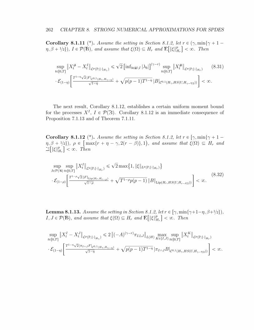
262 CHAPTER 8. STRONG NUMERICAL APPROXIMATIONS FOR SPDES
Corollary 8.1.11 (*). Assume the setting in Section 8.1.2, let r P pγ,mintγ ` 1 ´η, β ` 12uq, I P PpBq, and assume that ξpΩq Ď Hr and E
“
ξpHr‰
ă 8. Then
suptPr0,T s
›
›XB
t ´XIt
›
›
LppP;¨Hγ qď?
2“
infbPBzI |λb|‰pγ´rq
suptPr0,T s
›
›XB
t
›
›
LppP;¨Hr q(8.31)
¨ Ep1´ηq„
T 1´η?
2 |F |C0,1pHγ,Hγ´ηq?1´η
`a
ppp´ 1qT 1´η |B|C0,1pHγ ,HSpU,Hγ´η2qq
ă 8.
The next result, Corollary 8.1.12, establishes a certain uniform moment boundfor the processes XI , I P PpBq. Corollary 8.1.12 is an immediate consequence ofProposition 7.1.13 and of Theorem 7.1.11.
Corollary 8.1.12 (*). Assume the setting in Section 8.1.2, let r P rγ,mintγ ` 1 ´η, β ` 12uq, ρ P
“
maxtr ` η ´ γ, 2pr ´ βqu, 1˘
, and assume that ξpΩq Ď Hr andE“
ξpHr‰
ă 8. Then
supIPPpBq
suptPr0,T s
›
›XIt
›
›
LppP;¨Hr qď?
2 max
1, ξLppP;¨Hr q
(
¨ Ep1´ρq„
T 1´ρ?
2 F LippHr,Hr´ρq?1´ρ
`a
T 1´ρppp´ 1q BLippHr,HSpU,Hr´ρ2qq
ă 8.(8.32)
Lemma 8.1.13. Assume the setting in Section 8.1.2, let r P rγ,mintγ`1´η, β`12uq,I, J P PpBq, and assume that ξpΩq Ď Hr and E
“
ξpHr‰
ă 8. Then
suptPr0,T s
›
›XIt ´X
Jt
›
›
LppP;¨Hγ qď 2
›
›p´Aqpγ´rqπI4J›
›
LpHqmaxKPtI,Ju
suptPr0,T s
›
›XKt
›
›
LppP;¨Hr q
¨ Ep1´ηq„
T 1´η?
2 |πIXJF |C0,1pHγ,Hγ´ηq?1´η
`a
ppp´ 1qT 1´η |πIXJB|C0,1pHγ ,HSpU,Hγ´η2qq
ă 8.

8.1. SPATIAL SPECTRAL GALERKIN APPROXIMATIONS FOR SPDES 263
Proof of Lemma 8.1.13. Observe that
suptPr0,T s
›
›πIzJXIt ` πJzIX
Jt
›
›
2
LppP;¨Hγ qq“ sup
tPr0,T s
›
›πIzJXIt ` πJzIX
Jt
›
›
2
LppP;¨Hγ q
“ suptPr0,T s
›
›p´Aqpγ´rqπI4J p´Aqpr´γq
“
πIzJXIt ` πJzIX
Jt
‰›
›
2
LppP;¨Hγ q
ď›
›p´Aqpγ´rqπI4J›
›
2
LpHqsuptPr0,T s
›
›πIzJXIt ` πJzIX
Jt
›
›
2
LppP;¨Hr q
“›
›p´Aqpγ´rqπI4J›
›
2
LpHqsuptPr0,T s
›
›
›
›
›πIzJXIt ` πJzIX
Jt
›
›
2
Hr
›
›
›
Lp2pP;|¨|Rq
“›
›p´Aqpγ´rqπI4J›
›
2
LpHqsuptPr0,T s
›
›
›
›
›πIzJXIt
›
›
2
Hr`›
›πJzIXJt
›
›
2
Hr
›
›
›
Lp2pP;|¨|Rq
ď›
›p´Aqpγ´rqπI4J›
›
2
LpHqsuptPr0,T s
„
›
›
›
›
›πIzJXIt
›
›
2
Hr
›
›
›
Lp2pP;|¨|Rq`
›
›
›
›
›πJzIXJt
›
›
2
Hr
›
›
›
Lp2pP;|¨|Rq
“›
›p´Aqpγ´rqπI4J›
›
2
LpHqsuptPr0,T s
”
›
›πIzJXIt
›
›
2
LppP;¨Hr q`›
›πJzIXJt
›
›
2
LppP;¨Hr q
ı
.
(8.33)
Combining this with Lemma 8.1.10 completes the proof of Lemma 8.1.13.
Let us illustrate a bit different perspective on Lemma 8.1.13. For this assume thesetting in Section 8.1.2, let dr : PpBq ˆ PpBq Ñ r0,8q, r P p0,8q, be the mappingswhich satisfy for all I, J P PpBq, r P p0,8q that
drpI, Jq “›
›p´Aq´rπI4J›
›
LpHq, (8.34)
let r P pγ,mint1` γ ´ η, β ` 12uq, and assume ξpΩq Ď Hr and E“
ξpHr‰
ă 8. Exer-cise 8.1.14 then shows that the pair pPpBq, drq is a metric space and Lemma 8.1.13,in particular, ensures that the mapping1
pPpBq, dr´γq Q I ÞÑ XIP
´
Cpr0, T s, LppP; ¨Hγ qq, ¨Cpr0,T s,LppP;¨Hγ qq
¯
(8.35)
is globally Lipschitz continuous with a Lipschitz constant which is smaller or equal
1Clearly, the domain (the set of arguments) of the mapping (8.35) is not pPpBq, dr´γq but theset PpBq. The notation (8.35) is nonetheless used in order to emphasize the specific metric definedon the set PpBq of arguments. The same comment applies to the co-domain of the mapping (8.35).

264 CHAPTER 8. STRONG NUMERICAL APPROXIMATIONS FOR SPDES
than
2 ¨
«
supIPPpBq
suptPr0,T s
›
›XIt
›
›
LppP;¨Hr q
ff
(8.36)
¨ Ep1´ηq„
T 1´η?
2 |πIXJF |CC1pHγ,Hγ´ηq?1´η
`a
ppp´ 1qT 1´η |πIXJB|C0,1pHγ ,HSpU,Hγ´η2qq
ă 8.
Exercise 8.1.14 (*). Assume the setting in Section 8.1.2 and let dr : PpBqˆPpBq Ñr0,8q, r P p0,8q, be the mappings which satisfy for all I, J P PpBq, r P p0,8q that
drpI, Jq “›
›p´Aq´rπI4J›
›
LpHq. (8.37)
Prove that for every r P p0,8q it holds that the pair pPpBq, drq is a metric space.
Exercise 8.1.15 (Numerical estimates for strong convergence rates*). Let T “ 1,let pH, 〈¨, ¨〉H , ¨Hq “ pL2pBorelp0,1q; |¨|Rq, 〈¨, ¨〉L2pBorelp0,1q;|¨|Rq
, ¨L2pBorelp0,1q;|¨|Rqq, let
A : DpAq Ď H Ñ H be the Laplace operator with Dirichlet boundary conditions onH (see Definition 3.6.10), let en P H, n P N, satisfy for all n P N that en “rp?
2 sinpnπxqqxPp0,1qsP,BpHq, let pΩ,F ,P, pFtqtPr0,T sq be a stochastic basis, let pWtqtPr0,T s
be an IdH-cylindrical pΩ,F ,P, pFtqtPr0,T sq-Wiener process, let X : r0, T s ˆ Ω Ñ H bean pFtqtPr0,T s/BpHq-predictable stochastic process which fulfills for all t P r0, T s that
rXtsP,BpHq “
ż t
0
eApt´sq dWs, (8.38)
let πN P LpHq, N P N, satisfy for all N P N, v P H that πNpvq “řNn“1 〈en, v〉H en,
and let XN : r0, T s ˆ Ω Ñ πNpHq, N P N, be pFtqtPr0,T s/BpπNpHqq-predictablestochastic processes which satisfy for all N P N, t P r0, T s that
“
XNt
‰
P,BpHq “
ż t
0
πN eApt´sq dWs. (8.39)
Write a Matlab function which plots Monte Carlo approximations of the real num-
bers`
E“
X223
T ´ XNT
2H
‰˘12for N P t20, 21, 22, 23, . . . , 218, 219u. Hint: Use the fact
that for every N P N you can simulate exactly from XNT pPqBpHq.
Class exercise 8.1.16 (Convergence speed of spectral Galerkin approximations*).Assume the setting in Section 8.1.2 and assume that ξpΩq Ď Hγ`1 and E
“
ξpHγ`1
‰
ă
8. For which r P R does it holds that there exists a real number C P R such that forall I P PpBqztBu it holds that
suptPr0,T s
›
›XB
t ´XIt
›
›
LppP;¨Hγ qď C
“
infbPBzI |λb|‰´r
. (8.40)
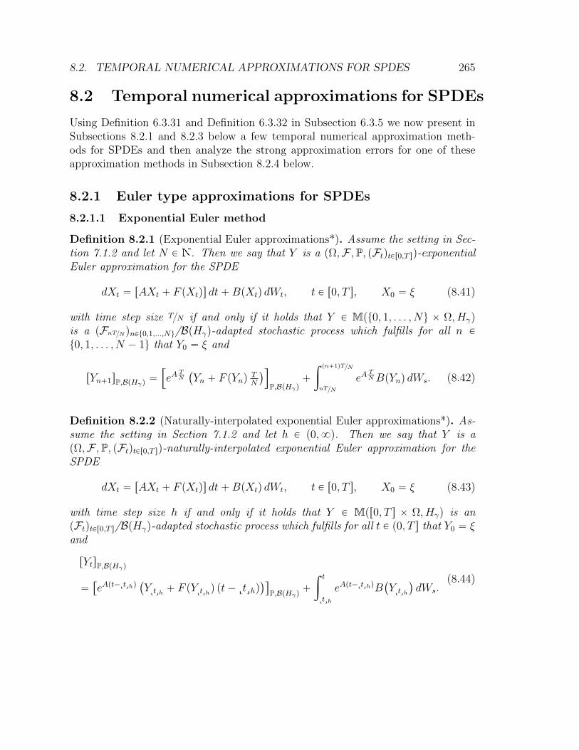
8.2. TEMPORAL NUMERICAL APPROXIMATIONS FOR SPDES 265
8.2 Temporal numerical approximations for SPDEs
Using Definition 6.3.31 and Definition 6.3.32 in Subsection 6.3.5 we now present inSubsections 8.2.1 and 8.2.3 below a few temporal numerical approximation meth-ods for SPDEs and then analyze the strong approximation errors for one of theseapproximation methods in Subsection 8.2.4 below.
8.2.1 Euler type approximations for SPDEs
8.2.1.1 Exponential Euler method
Definition 8.2.1 (Exponential Euler approximations*). Assume the setting in Sec-tion 7.1.2 and let N P N. Then we say that Y is a pΩ,F ,P, pFtqtPr0,T sq-exponentialEuler approximation for the SPDE
dXt “ rAXt ` F pXtqs dt`BpXtq dWt, t P r0, T s, X0 “ ξ (8.41)
with time step size TN if and only if it holds that Y P Mpt0, 1, . . . , Nu ˆ Ω, Hγq
is a pFnTNqnPt0,1,...,Nu/BpHγq-adapted stochastic process which fulfills for all n P
t0, 1, . . . , N ´ 1u that Y0 “ ξ and
rYn`1sP,BpHγq “”
eATN
`
Yn ` F pYnqTN
˘
ı
P,BpHγq`
ż pn`1qTN
nTN
eATNBpYnq dWs. (8.42)
Definition 8.2.2 (Naturally-interpolated exponential Euler approximations*). As-sume the setting in Section 7.1.2 and let h P p0,8q. Then we say that Y is apΩ,F ,P, pFtqtPr0,T sq-naturally-interpolated exponential Euler approximation for theSPDE
dXt “ rAXt ` F pXtqs dt`BpXtq dWt, t P r0, T s, X0 “ ξ (8.43)
with time step size h if and only if it holds that Y P Mpr0, T s ˆ Ω, Hγq is anpFtqtPr0,T s/BpHγq-adapted stochastic process which fulfills for all t P p0, T s that Y0 “ ξand
rYtsP,BpHγq
““
eApt´zthq`
Yzth ` F pYzthq pt´ zthq˘‰
P,BpHγq`
ż t
zth
eApt´zthqB`
Yzth
˘
dWs.(8.44)
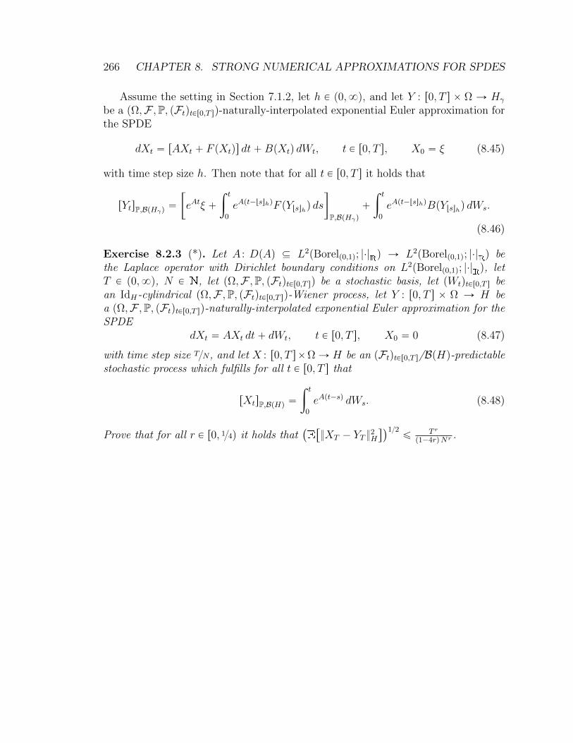
266 CHAPTER 8. STRONG NUMERICAL APPROXIMATIONS FOR SPDES
Assume the setting in Section 7.1.2, let h P p0,8q, and let Y : r0, T s ˆ Ω Ñ Hγ
be a pΩ,F ,P, pFtqtPr0,T sq-naturally-interpolated exponential Euler approximation forthe SPDE
dXt “ rAXt ` F pXtqs dt`BpXtq dWt, t P r0, T s, X0 “ ξ (8.45)
with time step size h. Then note that for all t P r0, T s it holds that
rYtsP,BpHγq “
„
eAtξ `
ż t
0
eApt´tsuhqF pYtsuhq ds
P,BpHγq`
ż t
0
eApt´tsuhqBpYtsuhq dWs.
(8.46)
Exercise 8.2.3 (*). Let A : DpAq Ď L2pBorelp0,1q; |¨|Rq Ñ L2pBorelp0,1q; |¨|Rq bethe Laplace operator with Dirichlet boundary conditions on L2pBorelp0,1q; |¨|Rq, letT P p0,8q, N P N, let pΩ,F ,P, pFtqtPr0,T sq be a stochastic basis, let pWtqtPr0,T s bean IdH-cylindrical pΩ,F ,P, pFtqtPr0,T sq-Wiener process, let Y : r0, T s ˆ Ω Ñ H bea pΩ,F ,P, pFtqtPr0,T sq-naturally-interpolated exponential Euler approximation for theSPDE
dXt “ AXt dt` dWt, t P r0, T s, X0 “ 0 (8.47)
with time step size TN, and let X : r0, T sˆΩ Ñ H be an pFtqtPr0,T s/BpHq-predictablestochastic process which fulfills for all t P r0, T s that
rXtsP,BpHq “
ż t
0
eApt´sq dWs. (8.48)
Prove that for all r P r0, 14q it holds that`
E“
XT ´ YT 2H
‰˘12ď T r
p1´4rqNr .

8.2. TEMPORAL NUMERICAL APPROXIMATIONS FOR SPDES 267
8.2.1.2 Accelerated exponential Euler method
Definition 8.2.4 (Accelerated exponential Euler approximations*). Assume the set-ting in Section 7.1.2 and let N P N. Then we say that Y is a pΩ,F ,P, pFtqtPr0,T sq-accelerated exponential Euler approximation for the SPDE
dXt “ rAXt ` F pXtqs dt`BpXtq dWt, t P r0, T s, X0 “ ξ (8.49)
with time step size TN if and only if it holds that Y P Mpt0, 1, . . . , Nu ˆ Ω, Hγq
is a pFnTNqnPt0,1,...,Nu/BpHγq-adapted stochastic process which fulfills for all n P
t0, 1, . . . , N ´ 1u that Y0 “ ξ and
rYn`1sP,BpHγq
“
”
eATN Yn ` A
´1`
eATN ´ IdH
˘
F pYnqı
P,BpHγq`
ż pn`1qTN
nTN
eAppn`1qTN´sqBpYnq dWs.
(8.50)
Definition 8.2.5 (Naturally-interpolated accelerated exponential Euler approxima-tions*). Assume the setting in Section 7.1.2 and let h P p0,8q. Then we say that Yis a pΩ,F ,P, pFtqtPr0,T sq-naturally-interpolated accelerated exponential Euler approx-imation for the SPDE
dXt “ rAXt ` F pXtqs dt`BpXtq dWt, t P r0, T s, X0 “ ξ (8.51)
with time step size h if and only if it holds that Y P Mpr0, T s ˆ Ω, Hγq is apFtqtPr0,T s/BpHγq-adapted stochastic process which fulfills for all t P p0, T s that Y0 “ ξand
rYtsP,BpHγq
“
„
eApt´zthq Yzth `
ż t
zth
eApt´sqF`
Yzth
˘
ds
P,BpHγq`
ż t
zth
eApt´sqB`
Yzth
˘
dWs.
(8.52)
Assume the setting in Section 7.1.2, let h P p0,8q, and let Y : r0, T sˆΩ Ñ Hγ bea pΩ,F ,P, pFtqtPr0,T sq-naturally-interpolated accelerated exponential Euler approxi-mation for the SPDE
dXt “ rAXt ` F pXtqs dt`BpXtq dWt, t P r0, T s, X0 “ ξ (8.53)
with time step size h. Then note that for all t P r0, T s it holds that
rYtsP,BpHγq “
„
eAtξ `
ż t
0
eApt´sqF`
Ytsuh
˘
ds
P,BpHγq`
ż t
0
eApt´sqB`
Ytsuh
˘
dWs. (8.54)

268 CHAPTER 8. STRONG NUMERICAL APPROXIMATIONS FOR SPDES
8.2.1.3 Linear-implicit Euler method
Definition 8.2.6 (Linear-implicit Euler approximations*). Assume the setting inSection 7.1.2 and let N P N. Then we say that Y is a pΩ,F ,P, pFtqtPr0,T sq-linear-implicit Euler approximation for the SPDE
dXt “ rAXt ` F pXtqs dt`BpXtq dWt, t P r0, T s, X0 “ ξ (8.55)
with time step size TN if and only if it holds that Y P Mpt0, 1, . . . , Nu ˆ Ω, Hγq
is a pFnTNqnPt0,1,...,Nu/BpHγq-adapted stochastic processes which fulfills for all n Pt0, 1, . . . , N ´ 1u that Y0 “ ξ and
rYn`1sP,BpHγq “”
`
IdH ´TNA˘´1 `
Yn ` F`
Yn˘
TN
˘
ı
P,BpHγq
`
ż pn`1qTN
nTN
`
IdH ´TNA˘´1
B`
Yn˘
dWs.(8.56)
Definition 8.2.7 (Naturally-interpolated linear-implicit Euler approximations*).Assume the setting in Section 7.1.2 and let h P p0,8q. Then we say that Y isa pΩ,F ,P, pFtqtPr0,T sq-naturally-interpolated linear-implicit Euler approximation forthe SPDE
dXt “ rAXt ` F pXtqs dt`BpXtq dWt, t P r0, T s, X0 “ ξ (8.57)
with time step size h if and only if it holds that Y P Mpr0, T s ˆ Ω, Hγq is apFtqtPr0,T s/BpHγq-adapted stochastic processes which fulfills for all t P p0, T s thatY0 “ ξ and
rYtsP,BpHγq ““
pIdH ´pt´ zthqAq´1
`
Yzth ` F`
Yzth
˘
pt´ zthq˘‰
P,BpHγq
`
ż t
zth
pIdH ´pt´ zthqAq´1B
`
Yzth
˘
dWs.(8.58)
Assume the setting in Section 7.1.2, let h P p0,8q, and let Y : r0, T s ˆ Ω Ñ Hγ
be a pΩ,F ,P, pFtqtPr0,T sq-naturally-interpolated linear-implicit Euler approximationfor the SPDE
dXt “ rAXt ` F pXtqs dt`BpXtq dWt, t P r0, T s, X0 “ ξ (8.59)
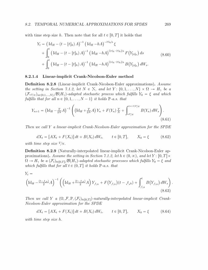
8.2. TEMPORAL NUMERICAL APPROXIMATIONS FOR SPDES 269
with time step size h. Then note that for all t P r0, T s it holds that
Yt “`
IdH ´pt´ ttuhqA˘´1 `
IdH ´hA˘´ttuhh
ξ
`
ż t
0
`
IdH ´pt´ ttuhqA˘´1 `
IdH ´hA˘ptsuh´ttuhqh
F`
Ytsuh
˘
ds
`
ż t
0
`
IdH ´pt´ ttuhqA˘´1 `
IdH ´hA˘ptsuh´ttuhqh
B`
Ytsuh
˘
dWs.
(8.60)
8.2.1.4 Linear-implicit Crank-Nicolson-Euler method
Definition 8.2.8 (Linear-implicit Crank-Nicolson-Euler approximations). Assumethe setting in Section 7.1.2, let N P N, and let Y : t0, 1, . . . , Nu ˆ Ω Ñ Hγ be apFnTNqnPt0,1,...,Nu/BpHγq-adapted stochastic process which fulfills Y0 “ ξ and whichfulfills that for all n P t0, 1, . . . , N ´ 1u it holds P-a.s. that
Yn`1 “`
IdH ´T
2NA˘´1
˜
`
IdH `T
2NA˘
Yn ` F pYnqTN`
ż pn`1qTN
nTN
BpYnq dWs
¸
.
(8.61)
Then we call Y a linear-implicit Crank-Nicolson-Euler approximation for the SPDE
dXt “ rAXt ` F pXtqs dt`BpXtq dWt, t P r0, T s, X0 “ ξ (8.62)
with time step size TN.
Definition 8.2.9 (Naturally-interpolated linear-implicit Crank-Nicolson-Euler ap-proximations). Assume the setting in Section 7.1.2, let h P p0,8q, and let Y : r0, T sˆΩ Ñ Hγ be a pFtqtPr0,T s/BpHγq-adapted stochastic processes which fulfills Y0 “ ξ andwhich fulfills that for all t P p0, T s it holds P-a.s. that
Yt “´
IdH ´pt´zthq
2A¯´1
ˆ
´
IdH `pt´zthq
2A¯
Yzth ` F`
Yzth
˘
pt´ zthq `
ż t
zth
B`
Yzth
˘
dWs
˙
.
(8.63)
Then we call Y a pΩ,F ,P, pFtqtPr0,T sq-naturally-interpolated linear-implicit Crank-Nicolson-Euler approximation for the SPDE
dXt “ rAXt ` F pXtqs dt`BpXtq dWt, t P r0, T s, X0 “ ξ (8.64)
with time step size h.

270 CHAPTER 8. STRONG NUMERICAL APPROXIMATIONS FOR SPDES
Assume the setting in Section 7.1.2, let h P p0,8q, and let Y : r0, T s ˆ Ω Ñ Hγ
be a pΩ,F ,P, pFtqtPr0,T sq-naturally-interpolated linear-implicit Euler approximationfor the SPDE
dXt “ rAXt ` F pXtqs dt`BpXtq dWt, t P r0, T s, X0 “ ξ (8.65)
with time step size h. Then note that for all t P r0, T s it holds P-a.s. that
Yt “`
IdH ´pt´ttuhq
2A˘´1 `
IdH ´h2A˘´ttuhh
ξ
`
ż t
0
`
IdH ´pt´ttuhq
2A˘´1 `
IdH ´h2A˘ptsuh´ttuhqh
“
12AYtsuh ` F
`
Ytsuh
˘‰
ds
`
ż t
0
`
IdH ´pt´ttuhq
2A˘´1 `
IdH ´h2A˘ptsuh´ttuhqh
B`
Ytsuh
˘
dWs.
(8.66)
8.2.2 Nonlinearity-stopped Euler type approximations forSPDEs
The next result is a special case of Theorem 2.1 in Hutzenthaler et al. [8] (see also[9]).
Theorem 8.2.10 (Strong and weak divergence of the Euler method for SDEs withsuperlinearly growing coefficients). Let T, ε, p P p0,8q, let pΩ,F ,P, pFtqtPr0,T sq bea stochastic basis, let W : r0, T s ˆ Ω Ñ R be a standard Brownian motion w.r.t.pFtqtPr0,T s, let µ, σ PMpBpRq,BpRqq, ξ PMpF0,BpRqq satisfy P
`
σpξq ‰ 0˘
ą 0, letY N : t0, 1, . . . , Nu ˆΩ Ñ R, N P N, satisfy that for all N P N, n P t0, 1, . . . , N ´ 1uit holds that Y N
0 “ ξ and
Y Nn`1 “ Y N
n ` µpY Nn q
TN` σpY N
n q`
Wpn`1qTN ´WnTN
˘
, (8.67)
and assume that for all x P p´8, 1εsYr1ε,8q it holds that |µpxq|`|σpxq| ě ε |x|p1`εq.Then limNÑ8 E
“
|Y NN |
p‰
“ 8.

8.2. TEMPORAL NUMERICAL APPROXIMATIONS FOR SPDES 271
8.2.2.1 Nonlinearity-stopped exponential Euler method
Definition 8.2.11 (Nonlinearity-stopped exponential Euler approximations). As-sume the setting in Section 7.1.2, let N P N, α P rγ´η, γs, assume that F pHγq Ď Hα,and let Y : t0, 1, . . . , NuˆΩ Ñ Hγ be an pFnTNqnPt0,1,...,Nu/BpHγq-adapted stochasticprocess which fulfills Y0 “ ξ and which fulfills that for all n P t0, 1, . . . , N ´ 1u itholds P-a.s. that
Yn`1 “ 1tF pYnq2HαąNTuYn
` 1tF pYnq2HαďNTueA
TN
˜
Yn ` F`
Yn˘
TN`
ż pn`1qTN
nTN
B`
Yn˘
dWs
¸
.(8.68)
Then we call Y a nonlinearity-stopped exponential Euler approximation for the SPDE
dXt “ rAXt ` F pXtqs dt`BpXtq dWt, t P r0, T s, X0 “ ξ (8.69)
with time step size TN.
Definition 8.2.12 (Naturally-interpolated nonlinearity-stopped exponential Eulerapproximations). Assume the setting in Section 7.1.2, let h P p0,8q, α P rγ ´ η, γs,assume that F pHγq Ď Hα, and let Y : r0, T sˆΩ Ñ Hγ be a pFtqtPr0,T s/BpHγq-adaptedstochastic process which fulfills Y0 “ ξ and which fulfills that for all t P p0, T s it holdsP-a.s. that
Yt “ 1tF pYzthq2Hα
ą1hu Yzth (8.70)
` 1tF pYzthq2αď1hu e
Apt´zthq
ˆ
Yzth ` F`
Yzth
˘
pt´ zthq `
ż t
zth
B`
Yzth
˘
dWs
˙
.
Then we call Y a pΩ,F ,P, pFtqtPr0,T sq-naturally-interpolated nonlinearity-stopped ex-ponential Euler approximation for the SPDE
dXt “ rAXt ` F pXtqs dt`BpXtq dWt, t P r0, T s, X0 “ ξ (8.71)
with time step size h.

272 CHAPTER 8. STRONG NUMERICAL APPROXIMATIONS FOR SPDES
8.2.2.2 Nonlinearity-stopped linear-implicit Euler method
Definition 8.2.13 (Nonlinearity-stopped linear-implicit Euler approximations). As-sume the setting in Section 7.1.2, let N P N, α P rγ´η, γs, assume that F pHγq Ď Hα,and let Y : t0, 1, . . . , Nu ˆ Ω Ñ Hγ be a pFnTNqnPt0,1,...,Nu/BpHγq-adapted stochasticprocess which fulfills Y0 “ ξ and which fulfills that for all n P t0, 1, . . . , N ´ 1u itholds P-a.s. that
Yn`1 “ 1tF pYnq2HαąNTuYn (8.72)
` 1tF pYnq2HαďNTu
`
IdH ´TNA˘´1
˜
Yn ` F`
Yn˘
TN`
ż pn`1qTN
nTN
B`
Yn˘
dWs
¸
.
Then we call Y a nonlinearity-stopped linear-implicit Euler approximation for theSPDE
dXt “ rAXt ` F pXtqs dt`BpXtq dWt, t P r0, T s, X0 “ ξ (8.73)
with time step size TN.
Definition 8.2.14 (Naturally-interpolated nonlinearity-stopped linear-implicit Eu-ler approximations). Assume the setting in Section 7.1.2, let h P p0,8q, α P rγ´η, γs,assume that F pHγq Ď Hα, and let Y : r0, T sˆΩ Ñ Hγ be a pFtqtPr0,T s/BpHγq-adaptedstochastic processes which fulfills Y0 “ ξ and which fulfills that for all t P p0, T s itholds P-a.s. that
Yt “ 1tF pYzthq2Hα
ą1hu Yzth ` 1tF pYzthq2Hα
ď1hu pIdH ´pt´ zthqAq´1
ˆ
Yzth
` F`
Yzth
˘
pt´ zthq `
ż t
zth
B`
Yzth
˘
dWs
˙
. (8.74)
Then we call Y a pΩ,F ,P, pFtqtPr0,T sq-naturally-interpolated nonlinearity-stopped linear-implicit Euler approximation for the SPDE
dXt “ rAXt ` F pXtqs dt`BpXtq dWt, t P r0, T s, X0 “ ξ (8.75)
with time step size h.

8.2. TEMPORAL NUMERICAL APPROXIMATIONS FOR SPDES 273
8.2.3 Milstein type approximations for SPDEs
8.2.3.1 Exponential Milstein method
Definition 8.2.15 (Exponential Milstein approximations*). Assume the setting inSection 7.1.2, assume that γ “ β, assume that B : Hγ Ñ HSpU,Hγq is continuouslyFrechet differentiable, and let N P N. Then we say that Y is a pΩ,F ,P, pFtqtPr0,T sq-exponential Milstein approximation for the SPDE
dXt “ rAXt ` F pXtqs dt`BpXtq dWt, t P r0, T s, X0 “ ξ (8.76)
with time step size TN if and only if it holds that Y P Mpt0, 1, . . . , Nu ˆ Ω, Hγq
is a pFnTNqnPt0,1,...,Nu/BpHγq-adapted stochastic processes which fulfills for all n Pt0, 1, . . . , N ´ 1u that Y0 “ ξ and
rYn`1sP,BpHγq “”
eATN
´
Yn ` F`
Yn˘
TN
¯ı
P,BpHγq`
żpn`1qTN
nTN
eATN B
`
Yn˘
dWs
`
żpn`1qTN
nTN
eATN B1
`
Yn˘
ˆż s
nTN
B`
Yn˘
dWu
˙
dWs
¸
.
(8.77)
Definition 8.2.16 (Naturally-interpolated exponential Milstein approximations).Assume the setting in Section 7.1.2, assume that γ “ β, assume that B : Hγ Ñ
HSpU,Hγq is continuously Frechet differentiable, and let h P p0,8q. Then we saythat Y is a pΩ,F ,P, pFtqtPr0,T sq-naturally-interpolated exponential Milstein approxi-mation for the SPDE
dXt “ rAXt ` F pXtqs dt`BpXtq dWt, t P r0, T s, X0 “ ξ (8.78)
with time step size h if and only if it holds that Y P Mpr0, T s ˆ Ω, Hγq is apFtqtPr0,T s/BpHγq-adapted stochastic process which fulfills for all t P p0, T s that Y0 “ ξand
rYtsP,BpHγq “
„
eApt´zthq
ˆ
Yzth ` F`
Yzth
˘
pt´ zthq
P,BpHγq
`
ż t
zth
”
B`
Yzth
˘
`B1`
Yzth
˘s
∫zth
B`
Yzth
˘
dWu
ı
dWs
˙
.
(8.79)

274 CHAPTER 8. STRONG NUMERICAL APPROXIMATIONS FOR SPDES
Assume the setting in Section 7.1.2, let h P p0,8q, and let Y : r0, T s ˆ Ω Ñ Hγ
be a pΩ,F ,P, pFtqtPr0,T sq-naturally-interpolated exponential Milstein approximationfor the SPDE
dXt “ rAXt ` F pXtqs dt`BpXtq dWt, t P r0, T s, X0 “ ξ (8.80)
with time step size h. Then note that for all t P r0, T s it holds that
rYtsP,BpHγq “
„
eAtξ `
ż t
0
eApt´tsuhqF`
Ytsuh
˘
ds
P,BpHγq
`
ż t
0
eApt´tsuhq”
B`
Ytsuh
˘
`B1`
Ytsuh
˘s
∫tsuh
BpYtsuhq dWu
ı
dWs.
(8.81)
8.2.3.2 Linear-implicit Milstein method
Definition 8.2.17 (Linear-implicit Milstein approximations). Assume the settingin Section 7.1.2, assume that γ “ β, assume that B : Hγ Ñ HSpU,Hγq is contin-uously Frechet differentiable, let N P N, and let Y : t0, 1, . . . , Nu ˆ Ω Ñ Hγ be apFnTNqnPt0,1,...,Nu/BpHγq-adapted stochastic processes which fulfills Y0 “ ξ and whichfulfills that for all n P t0, 1, . . . , N ´ 1u it holds P-a.s. that
Yn`1 “`
IdH ´TNA˘´1
˜
Yn ` F`
Yn˘
TN`
żpn`1qTN
nTN
B`
Yn˘
dWs
`
żpn`1qTN
nTN
B1`
Yn˘
ˆż s
nTN
B`
Yn˘
dWu
˙
dWs
¸
.
(8.82)
Then we call Y a linear-implicit Milstein approximation for the SPDE
dXt “ rAXt ` F pXtqs dt`BpXtq dWt, t P r0, T s, X0 “ ξ (8.83)
with time step size TN.

8.2. TEMPORAL NUMERICAL APPROXIMATIONS FOR SPDES 275
Definition 8.2.18 (Naturally-interpolated linear-implicit Milstein approximations).Assume the setting in Section 7.1.2, assume that γ “ β, assume that B : Hγ Ñ
HSpU,Hγq is continuously Frechet differentiable, let h P p0,8q, and let Y : r0, T s ˆΩ Ñ Hγ be an pFtqtPr0,T s/BpHγq-adapted stochastic processes which fulfills Y0 “ ξand which fulfills that for all t P p0, T s it holds P-a.s. that
Yt “pIdH ´pt´ zthqAq´1
ˆ
Yzth ` F`
Yzth
˘
pt´ zthq
`
ż t
zth
”
B`
Yzth
˘
`B1`
Yzth
˘s
∫zth
B`
Yzth
˘
dWu
ı
dWs
˙
.
(8.84)
Then we call Y a pΩ,F ,P, pFtqtPr0,T sq-naturally-interpolated linear-implicit Milsteinapproximation for the SPDE
dXt “ rAXt ` F pXtqs dt`BpXtq dWt, t P r0, T s, X0 “ ξ (8.85)
with time step size h.
Assume the setting in Section 7.1.2, let h P p0,8q, and let Y : r0, T sˆΩ Ñ Hγ bea pΩ,F ,P, pFtqtPr0,T sq-naturally-interpolated linear-implicit Milstein approximationfor the SPDE
dXt “ rAXt ` F pXtqs dt`BpXtq dWt, t P r0, T s, X0 “ ξ (8.86)
with time step size h. Then note that for all t P r0, T s it holds P-a.s. that
Yt “`
IdH ´pt´ ttuhqA˘´1 `
IdH ´hA˘´ttuhh
ξ
`
ż t
0
`
IdH ´pt´ ttuhqA˘´1 `
IdH ´hA˘ptsuh´ttuhqh
F`
Ytsuh
˘
ds
`
ż t
0
`
IdH ´pt´ ttuhqA˘´1 `
IdH ´hA˘ptsuh´ttuhqh
B`
Ytsuh
˘
dWs
`
ż t
0
`
IdH ´pt´ ttuhqA˘´1 `
IdH ´hA˘ptsuh´ttuhqh
”
B1`
Yttuh
˘s
∫ttuh
B`
Yttuh
˘
dWu
ı
dWs.
(8.87)

276 CHAPTER 8. STRONG NUMERICAL APPROXIMATIONS FOR SPDES
8.2.3.3 Linear-implicit Crank-Nicolson-Milstein method
Definition 8.2.19 (Linear-implicit Crank-Nicolson-Milstein approximations). As-sume the setting in Section 7.1.2, assume that γ “ β, assume that B : Hγ Ñ
HSpU,Hγq is continuously Frechet differentiable, let N P N, and let Y : t0, 1, . . . , NuˆΩ Ñ Hγ be a pFnTNqnPt0,1,...,Nu/BpHγq-adapted stochastic processes which fulfillsY0 “ ξ and which fulfills that for all n P t0, 1, . . . , N ´ 1u it holds P-a.s. that
Yn`1 “`
IdH ´T
2NA˘´1
˜
`
IdH `T
2NA˘
Yn ` F`
Yn˘
TN`
żpn`1qTN
nTN
B`
Yn˘
dWs
`
żpn`1qTN
nTN
B1`
Yn˘
ˆż s
nTN
B`
Yn˘
dWu
˙
dWs
¸
. (8.88)
Then we call Y a pΩ,F ,P, pFtqtPr0,T sq-naturally-interpolated linear-implicit Crank-Nicolson-Milstein approximation for the SPDE
dXt “ rAXt ` F pXtqs dt`BpXtq dWt, t P r0, T s, X0 “ ξ (8.89)
with time step size h.
Definition 8.2.20 (Naturally-interpolated linear-implicit Crank-Nicolson-Milsteinapproximations). Assume the setting in Section 7.1.2, assume that γ “ β, assumethat B : Hγ Ñ HSpU,Hγq is continuously Frechet differentiable, let h P p0,8q, andlet Y : r0, T s ˆ Ω Ñ Hγ be a pFtqtPr0,T s/BpHγq-adapted stochastic processes whichfulfills Y0 “ ξ and which fulfills that for all t P p0, T s it holds P-a.s. that
Yt “`
IdH ´12pt´ zthqA
˘´1
ˆ
Yzth `12AYzth pt´ zthq ` F
`
Yzth
˘
pt´ zthq
`
ż t
zth
”
B`
Yzth
˘
`B1`
Yzth
˘s
∫zth
B`
Yzth
˘
dWu
ı
dWs
˙
.
(8.90)
Then we call Y a pΩ,F ,P, pFtqtPr0,T sq-naturally-interpolated linear-implicit Crank-Nicolson-Milstein approximation for the SPDE
dXt “ rAXt ` F pXtqs dt`BpXtq dWt, t P r0, T s, X0 “ ξ (8.91)
with time step size h.

8.2. TEMPORAL NUMERICAL APPROXIMATIONS FOR SPDES 277
Assume the setting in Section 7.1.2, let h P p0,8q, and let Y : r0, T sˆΩ Ñ Hγ bea pΩ,F ,P, pFtqtPr0,T sq-naturally-interpolated linear-implicit Crank-Nicolson-Milsteinapproximation for the SPDE
dXt “ rAXt ` F pXtqs dt`BpXtq dWt, t P r0, T s, X0 “ ξ (8.92)
with time step size h. Then note that for all t P r0, T s it holds P-a.s. that
Yt “`
IdH ´pt´ttuhq
2A˘´1 `
IdH ´h2A˘´ttuhh
ξ
`
ż t
0
`
IdH ´pt´ttuhq
2A˘´1 `
IdH ´h2A˘ptsuh´ttuhqh
”
12AYtsuh ` F
`
Ytsuh
˘
ı
ds
`
ż t
0
`
IdH ´pt´ttuhq
2A˘´1 `
IdH ´h2A˘ptsuh´ttuhqh
B`
Ytsuh
˘
dWs
`
ż t
0
`
IdH ´pt´ttuhq
2A˘´1 `
IdH ´h2A˘ptsuh´ttuhqh
”
B1`
Yttuh
˘s
∫ttuh
B`
Yttuh
˘
dWu
ı
dWs.
(8.93)
8.2.4 Strong convergence analysis for exponential Euler ap-proximations
In this subsection we establish strong convergence with suitable rates of convergenceof exponential Euler approximations; see Definition 8.2.1. In this subsection wemainly follow the analysis in Kurniawan [16].
Lemma 8.2.21 (Regularity for the numerical approximations*). Assume the settingin Subsection 7.1.2, let N P N, and let Y : r0, T sˆΩ Ñ Hγ be a pΩ,F ,P, pFtqtPr0,T sq-naturally-interpolated exponential Euler approximation for the SPDE
dXt “ rAXt ` F pXtqs dt`BpXtq dWt, t P r0, T s, X0 “ ξ (8.94)
with time step size TN. Then
suptPr0,T s
YtLppP;¨Hγ qď max
1,?
2 ξLppP;¨Hγ q
(
(8.95)
¨ E1´η
„
T 1´η?
2 F LippHγ,Hγ´ηq?1´η
`a
T 1´η p pp´ 1q BLippHγ ,HSpU,Hγ´η2qq
ă 8.

278 CHAPTER 8. STRONG NUMERICAL APPROXIMATIONS FOR SPDES
Proof of Lemma 8.2.21*. Theorem 4.8.5 and Holder’s inequality imply that for allt P r0, T s it holds that
YtLppP;¨Hγ qď ξLppP;¨Hγ q
` F LippHγ ,Hγ´ηq
„
tp1´ηq
p1´ηq
ż t
0
pt´ sq´η max
1,›
›YtsuT N
›
›
2
LppP;¨Hγ q
(
ds
12
` BLippHγ ,HSpU,Hγ´η2qq
„
ppp´1q2
ż t
0
pt´ sq´η max
1,›
›YtsuT N
›
›
2
LppP;¨Hγ q
(
ds
12
.
(8.96)
This proves that for all t P r0, T s it holds that
YtLppP;¨Hγ qď ξLppP;¨Hγ q
`
„ż t
0
pt´ sq´η max
1,›
›YtsuT N
›
›
2
LppP;¨Hγ q
(
ds
12
¨
„
F LippHγ ,Hγ´ηqTp1´ηq2?
1´η` BLippHγ ,HSpU,Hγ´η2qq
?ppp´1q?
2
.
(8.97)
Induction hence proves that for all t P r0, T s it holds that YtLppP;¨Hγ qă 8.
Moreover, combining (8.97) with the estimate that for all a, b P R it holds thatpa` bq2 ď 2a2 ` 2b2 shows that for all t P r0, T s it holds that
max
1, Yt2LppP;¨Hγ q
(
ď max
1, 2 ξ2LppP;¨Hγ q
(
`
ż t
0
pt´ sq´η max
1,›
›YtsuT N
›
›
2
LppP;¨Hγ q
(
ds
¨
”
F LippHγ ,Hγ´ηq
?2T
p1´ηq2?
1´η` BLippHγ ,HSpU,Hγ´η2qq
a
p pp´ 1qı2
.
(8.98)

8.2. TEMPORAL NUMERICAL APPROXIMATIONS FOR SPDES 279
Next note that for all u P r0, T s it holds that
suptPr0,us
ż t
0
pt´ sq´η max
1,›
›YtsuT N
›
›
2
LppP;¨Hγ q
(
ds
ď suptPr0,us
ż t
0
pt´ sq´η”
supvPr0,ss max
1, Yv2LppP;¨Hγ q
(
ı
ds
“ suptPr0,us
ż u
u´t
pt´ rs´ pu´ tqsq´η”
supvPr0,s´pu´tqs max
1, Yv2LppP;¨Hγ q
(
ı
ds
“ suptPr0,us
ż u
u´t
pu´ sq´η”
supvPr0,s`t´us max
1, Yv2LppP;¨Hγ q
(
ı
ds
ď suptPr0,us
ż u
u´t
pu´ sq´η”
supvPr0,ss max
1, Yv2LppP;¨Hγ q
(
ı
ds
“
ż u
0
pu´ sq´η”
supvPr0,ss max
1, Yv2LppP;¨Hγ q
(
ı
ds.
(8.99)
Putting this into (8.98) proves that for all u P r0, T s it holds that
suptPr0,us max
1, Yt2LppP;¨Hγ q
(
ď max
1, 2 ξ2LppP;¨Hγ q
(
`
ż u
0
pu´ sq´η”
suptPr0,ss max
1, Yt2LppP;¨Hγ q
(
ı
ds
¨
”
F LippHγ ,Hγ´ηq
?2T
p1´ηq2?
1´η` BLippHγ ,HSpU,Hγ´η2qq
a
p pp´ 1qı2
.
(8.100)
Combining this with Corollary 1.4.6 completes the proof of Lemma 8.2.21.

280 CHAPTER 8. STRONG NUMERICAL APPROXIMATIONS FOR SPDES
Lemma 8.2.22 (More regularity for the numerical approximation processes*). As-sume the setting in Subsection 7.1.2, let N P N, and let Y : r0, T s ˆ Ω Ñ Hγ bea pΩ,F ,P, pFtqtPr0,T sq-naturally-interpolated exponential Euler approximation for theSPDE
dXt “ rAXt ` F pXtqs dt`BpXtq dWt, t P r0, T s, X0 “ ξ (8.101)
with time step size TN. Then
(i) it holds for all t P r0, T s, r P rγ,mint1 ` γ ´ η, 12 ` βuq that P`
Yt ´ eAtY0 P
Hr
˘
“ 1 and
›
›Yt ´ eAtY0
›
›
LppP;¨Hr qď max
#
1, supnPt0,1,...,Nu
YnTNLppP;¨Hγ q
+
¨
«
F LippHγ ,Hγ´ηqtp1`γ´η´rq
p1` γ ´ η ´ rq`
a
p pp´ 1q BLippHγ ,HSpU,Hβqqtp12`β´rq
p2` 4β ´ 4rq12
ff
ă 8
(8.102)
and
(ii) it holds for all t P p0, T s, r P rγ,mint1 ` γ ´ η, 12 ` βuq that P`
Yt P Hr
˘
“ 1and
YtLppP;¨Hr qď
X0LppP;¨Hγ q
tpr´γq`max
!
1, supnPt0,1,...,Nu YnTNLppP;¨Hγ q
)
¨
„
F LippHγ,Hγ´ηqtp1`γ´η´rq
p1`γ´η´rq`
?p pp´1q BLippHγ,HSpU,Hβqq
tp12`β´rq
p2`4β´4rq12
ă 8.
(8.103)
Proof of Lemma 8.2.22*. First of all, recall that for all t P r0, T s it holds that
“
Yt ´ eAtY0
‰
P,BpHγq
“
„ż t
0
eApt´tsuT N qF pYtsuT Nq ds
P,BpHγq`
ż t
0
eApt´tsuT N qBpYtsuT Nq dWs.
(8.104)
Moreover, note that Theorem 4.8.5 implies that for all t P r0, T s, r P rγ, γ ` 1´ ηq it

8.2. TEMPORAL NUMERICAL APPROXIMATIONS FOR SPDES 281
holds that
ż t
0
›
›
›eApt´tsuT N qF pYtsuT N
q
›
›
›
LppP;¨Hr qds
ď F LippHγ ,Hγ´ηqmax
#
1, supsPr0,T s
YtsuT NLppP;¨Hγ q
+
„ż t
0
pt´ sqpγ´η´rq ds
“ F LippHγ ,Hγ´ηqmax
#
1, supsPr0,T s
YtsuT NLppP;¨Hγ q
+
tp1`γ´η´rq
p1` γ ´ η ´ rqă 8.
(8.105)
Furthermore, observe that Theorem 4.8.5 ensures that for all t P r0, T s, r P rγ, β`12q
it holds that
„ż t
0
›
›
›eApt´tsuT N qBpYtsuT N
q
›
›
›
2
LppP;¨HSpU,Hrqqds
12
ď BLippHγ ,HSpU,Hβqqmax
#
1, supsPr0,T s
YtsuT NLppP;¨Hγ q
+
„ż t
0
pt´ sqp2β´2rq ds
12
ď BLippHγ ,HSpU,Hβqqmax
#
1, supsPr0,T s
YtsuT NLppP;¨Hγ q
+
tp12`β´rq
p1` 2β ´ 2rq12ă 8.
(8.106)
Combining (8.104), (8.105), and (8.106) with Theorem 4.8.5 and Theorem 6.3.29completes the proof of Lemma 8.2.22.
Lemma 8.2.23 (Regularity of a time integral associated to the numerical approx-imations*). Assume the setting in Section 7.1.2, let ρ P r0, 1q, q P r1,8q, and forevery N P N let Y N : r0, T sˆΩ Ñ Hγ be a pΩ,F ,P, pFtqtPr0,T sq-naturally-interpolatedexponential Euler approximation for the SPDE
dXt “ rAXt ` F pXtqs dt`BpXtq dWt, t P r0, T s, X0 “ ξ (8.107)
with time step size TN. Then it holds for all r P p´8,mintp1´ρqq, 1´ η, 12` β ´ γuqthat
supNPN
suptPr0,T s
„
N rt
∫0pt´ sq´ρ
›
›
›Y Ns ´ Y N
tsuT N
›
›
›
q
LppP;¨Hγ qds
1q
ă 8. (8.108)

282 CHAPTER 8. STRONG NUMERICAL APPROXIMATIONS FOR SPDES
Proof of Lemma 8.2.23*. First of all, observe that for all N P N it holds that
suptPr0,TNs
„
t
∫0pt´ sq´ρ
›
›
›Y Ns ´ Y N
tsuT N
›
›
›
q
LppP;¨Hγ qds
1q
ď
2 suptPp0,T s›
›Y Nt
›
›
LppP;¨Hγ qT p1´ρqq
p1´ ρq1qN p1´ρqq.
(8.109)
Next note that for all r P rγ,mint1 ` γ ´ η, 12 ` βuq, N P N, t P rTN, T s it holdsthat
„
t
∫0pt´ sq´ρ
›
›
›Y Ns ´ Y N
tsuT N
›
›
›
q
LppP;¨Hγ qds
1q
ď 2 supsPp0,T s
›
›Y Ns
›
›
LppP;¨Hγ q
„
TN
∫0pt´ sq´ρ ds
1q
`
«
supsPrTN,T s
`
tsuT N˘pr´γq
›
›
›Y Ns ´ Y N
tsuT N
›
›
›
LppP;¨Hγ q
ff«
t
∫TN
pt´ sq´ρ
`
tsuT N˘q pr´γq
ds
ff1q
ď 2 supsPp0,T s
›
›Y Ns
›
›
LppP;¨Hγ q
T p1´ρqq
N p1´ρqq p1´ ρq1q
`
«
supsPrTN,T s
`
tsuT N˘pr´γq
›
›
›Y Ns ´ Y N
tsuT N
›
›
›
LppP;¨Hγ q
ff
„
t´TN
∫0
pt´ TN ´ sq´ρ
sq pr´γqds
1q
.
(8.110)
This implies that that for all r P rγ,mint1` γ´ η, 12`βuq, N P N, t P rTN, T s withρ` qpr ´ γq ď 1 it holds that
„
t
∫0pt´ sq´ρ
›
›
›Y Ns ´ Y N
tsuT N
›
›
›
q
LppP;¨Hγ qds
1q
ď
2 supsPp0,T s›
›Y Ns
›
›
LppP;¨Hγ qT p1´ρqq
N p1´ρqq p1´ ρq1q
`
«
supsPrTN,T s
`
tsuT N˘pr´γq
›
›
›Y Ns ´ Y N
tsuT N
›
›
›
LppP;¨Hγ q
ff
¨ rt´ TNsr1´ρq´pr´γqs
“
B`
1´ ρ, 1´ qpr ´ γq˘‰1q
.
(8.111)
Combining this with (8.109) proves that for all r P rγ,mintγ`p1´ρqq, γ`1´η, 12`βuq,

8.2. TEMPORAL NUMERICAL APPROXIMATIONS FOR SPDES 283
N P N it holds that
suptPr0,T s
„
t
∫0pt´ sq´ρ
›
›
›Y Ns ´ Y N
tsuT N
›
›
›
q
LppP;¨Hγ qds
1q
ď
2 supsPp0,T s›
›Y Ns
›
›
LppP;¨Hγ qT p1´ρqq
N p1´ρqq p1´ ρq1q
`
«
supsPrTN,T s
`
tsuT N˘pr´γq
›
›
›Y Ns ´ Y N
tsuT N
›
›
›
LppP;¨Hγ q
ff
¨ T rγ`p1´ρqq´rs
“
B`
1´ ρ, 1´ qpr ´ γq˘‰1q
.
(8.112)
In the next step we observe that Theorem 6.3.29, Lemma 4.8.6 and Lemma 8.2.22ensure that for all N P N, s P rTN, T s, r P rγ,mint1` γ ´ η, 12` βuq it holds that
›
›
›Y Ns ´ Y N
tsuT N
›
›
›
LppP;¨Hγ qď
›
›
›
`
eAps´tsuT N q ´ IdH˘
Y NtsuT N
›
›
›
LppP;¨Hγ q
`
ż s
tsuT N
›
›eAps´tuuT N qF pY NtuuT N
q›
›
LppP;¨Hγ qdu
`
«
p pp´ 1q
2
ż s
tsuT N
›
›
›eAps´tuuT N qBpY N
tuuT Nq
›
›
›
2
LppP;¨HSpU,Hγ qqdu
ff12
ď`
s´ tsuT N˘pr´γq
›
›
›Y N
tsuT N
›
›
›
LppP;¨Hr q
`
ż s
tsuT N
ps´ uq´η›
›
›F pY N
tuuT Nq
›
›
›
LppP;¨Hγ´ηqdu
`
«
p pp´ 1q
2
ż s
tsuT N
ps´ uqp2β´2γq›
›
›BpY N
tuuT Nq
›
›
›
2
LppP;¨HSpU,Hβqqdu
ff12
ă 8.
(8.113)
This implies that for all N P N, s P rTN, T s, r P rγ,mint1` γ ´ η, 12` βuq it holdsthat›
›
›Y Ns ´ Y N
tsuT N
›
›
›
LppP;¨Hγ qď
„
T
N
pr´γqˇ
ˇtsuT Nˇ
ˇ
pγ´rq
«
supuPp0,T s
upr´γq›
›Y Nu
›
›
LppP;¨Hr q
ff
`“
TN
‰p1´ηq F LippHγ,Hγ´ηq
p1´ηqmax
"
1, supnPt1,2,...,Nu›
›Y NnTN
›
›
LppP;¨Hγ q
*
`“
TN
‰p12`β´γq BLippHγ,HSpU,Hβqq
p1`2β´2γq12
”
p pp´1q2
ı12
max
"
1, supnPt1,2,...,Nu›
›Y NnTN
›
›
LppP;¨Hγ q
*
.
(8.114)

284 CHAPTER 8. STRONG NUMERICAL APPROXIMATIONS FOR SPDES
This shows that for all N P N, r P rγ,mint1` γ ´ η, 12` βuq it holds that
supsPrTN,T s
„
ˇ
ˇtsuT Nˇ
ˇ
pr´γq›
›
›Y Ns ´ Y N
tsuT N
›
›
›
LppP;¨Hγ q
ď
”
“
TN
‰pr´γq`“
TN
‰p1´ηq Tpr´γq F LippHγ,Hγ´ηq
p1´ηq
`“
TN
‰p12`β´γq Tpr´γq BLippHγ,HSpU,Hβqq
p12`β´γq12
”
p pp´1q4
ı12 ı
¨max
#
1, supvPrγ,rs
supuPp0,T s
upv´γq›
›Y Nu
›
›
LppP;¨Hv q
+
.
(8.115)
Putting this into (8.112) proves that for all N P N, r P rγ,mintγ ` p1´ρqq, γ ` 1 ´η, 12` βuq it holds that
suptPr0,T s
„
t
∫0pt´ sq´ρ
›
›
›Y Ns ´ Y N
tsuT N
›
›
›
q
LppP;¨Hγ qds
1q
ď
«
2T p1´ρqq
N p1´ρqq p1´ ρq1q
`
”
1`T p1´ηq F LippHγ,Hγ´ηq
p1´ηq`
T p12`β´γq BLippHγ,HSpU,Hβqq
p12`β´γq12
”
p pp´1q4
ı12 ı
¨T p1´ρqq
N pr´γq
“
B`
1´ ρ, 1´ qpr ´ γq˘‰1q
ff
¨max
#
1, supvPrγ,rs
supuPp0,T s
upv´γq›
›Y Nu
›
›
LppP;¨Hv q
+
.
(8.116)
Hence, we obtain that for all N P N, r P rγ,mintγ ` p1´ρqq, γ ` 1 ´ η, 12 ` βuq itholds that
suptPr0,T s
„
t
∫0pt´ sq´ρ
›
›
›Y Ns ´ Y N
tsuT N
›
›
›
q
LppP;¨Hγ qds
1q
ď
„
52` F LippHγ ,Hγ´ηq ` BLippHγ ,HSpU,Hβqq
?p pp´1q
2
¨
“
B`
1´ ρ, 1´ qpr ´ γq˘‰1q
maxpT 2, 1q
mint1´ ρ, 1´ η, 12` β ´ γuN pr´γqmax
#
1, supvPrγ,rs
supuPp0,T s
upv´γq›
›Y Nu
›
›
LppP;¨Hv q
+
.
(8.117)
This and Lemma 8.2.22 complete the proof of Lemma 8.2.23.
In the next result, Corollary 8.2.24, an estimate for the strong approximationerror of exponential Euler approximations is presented.

8.2. TEMPORAL NUMERICAL APPROXIMATIONS FOR SPDES 285
Corollary 8.2.24 (*). Assume the setting in Section 7.1.2, let X : r0, T s ˆΩ Ñ Hγ
be a stochastic process which satisfies suptPr0,T s XtLppP;¨Hγ qă 8 and which is a
pΩ,F ,P, pFtqtPr0,T sq-mild solution of the SPDE
dXt “ rAXt ` F pXtqs dt`BpXtq dWt, t P r0, T s, X0 “ ξ, (8.118)
let N P N, and let Y : r0, T sˆΩ Ñ Hγ be a pΩ,F ,P, pFtqtPr0,T sq-naturally-interpolatedexponential Euler approximation for the SPDE (8.118) with time step size TN. Then
suptPr0,T s
Xt ´ YtLppP;¨Hγ q
ď Ep1´ηq„
T 1´η?
2 |F |C0,1pHγ,Hγ´ηq?1´η
`a
T 1´ηppp´ 1q |B|C0,1pHγ ,HSpU,Hγ´η2qq
¨?
2 suptPr0,T s
«
ż t
0
›
›
›eApt´sq
”
F pYsq ´ eAps´tsuT N qF pYtsuT N
q
ı›
›
›
LppP;¨Hγ qds
`
„
p pp´1q2
t
∫0
›
›
›eApt´sq
”
BpYsq ´ eAps´tsuT N qBpYtsuT N
q
ı›
›
›
2
LppP;¨HSpU,Hγ qqds
12ff
ă 8.
(8.119)
Corollary 8.2.24 is an immediate consequence of Proposition 7.1.6 and of Theo-rem 6.3.29.
Theorem 8.2.25 (*). Assume the setting in Section 7.1.2, let X : r0, T s ˆ Ω Ñ Hγ
be a stochastic process which satisfies suptPr0,T s XtLppP;¨Hγ qă 8 and which is a
pΩ,F ,P, pFtqtPr0,T sq-mild solution of the SPDE
dXt “ rAXt ` F pXtqs dt`BpXtq dWt, t P r0, T s, X0 “ ξ, (8.120)
and for every N P N let Y N : r0, T s ˆ Ω Ñ Hγ be a pΩ,F ,P, pFtqtPr0,T sq-naturally-interpolated exponential Euler approximation for the SPDE (8.120) with time stepsize TN. Then it holds for all r P
`
´8,mint1´ η, 12` β ´ γu˘
that
supNPN
suptPr0,T s
„
N r›
›Xt ´ YNt
›
›
LppP;¨Hγ q
ă 8. (8.121)
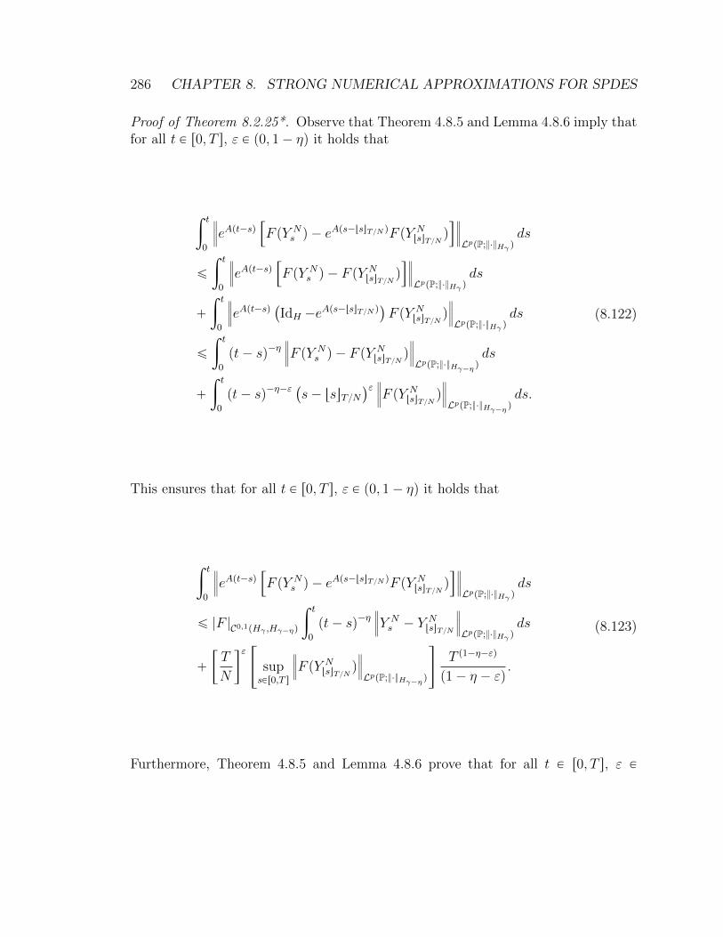
286 CHAPTER 8. STRONG NUMERICAL APPROXIMATIONS FOR SPDES
Proof of Theorem 8.2.25*. Observe that Theorem 4.8.5 and Lemma 4.8.6 imply thatfor all t P r0, T s, ε P p0, 1´ ηq it holds that
ż t
0
›
›
›eApt´sq
”
F pY Ns q ´ e
Aps´tsuT N qF pY NtsuT N
q
ı›
›
›
LppP;¨Hγ qds
ď
ż t
0
›
›
›eApt´sq
”
F pY Ns q ´ F pY
NtsuT N
q
ı›
›
›
LppP;¨Hγ qds
`
ż t
0
›
›
›eApt´sq
`
IdH ´eAps´tsuT N q
˘
F pY NtsuT N
q
›
›
›
LppP;¨Hγ qds
ď
ż t
0
pt´ sq´η›
›
›F pY N
s q ´ F pYN
tsuT Nq
›
›
›
LppP;¨Hγ´η qds
`
ż t
0
pt´ sq´η´ε`
s´ tsuT N˘ε›
›
›F pY N
tsuT Nq
›
›
›
LppP;¨Hγ´η qds.
(8.122)
This ensures that for all t P r0, T s, ε P p0, 1´ ηq it holds that
ż t
0
›
›
›eApt´sq
”
F pY Ns q ´ e
Aps´tsuT N qF pY NtsuT N
q
ı›
›
›
LppP;¨Hγ qds
ď |F |C0,1pHγ ,Hγ´ηq
ż t
0
pt´ sq´η›
›
›Y Ns ´ Y N
tsuT N
›
›
›
LppP;¨Hγ qds
`
„
T
N
ε«
supsPr0,T s
›
›
›F pY N
tsuT Nq
›
›
›
LppP;¨Hγ´η q
ff
T p1´η´εq
p1´ η ´ εq.
(8.123)
Furthermore, Theorem 4.8.5 and Lemma 4.8.6 prove that for all t P r0, T s, ε P
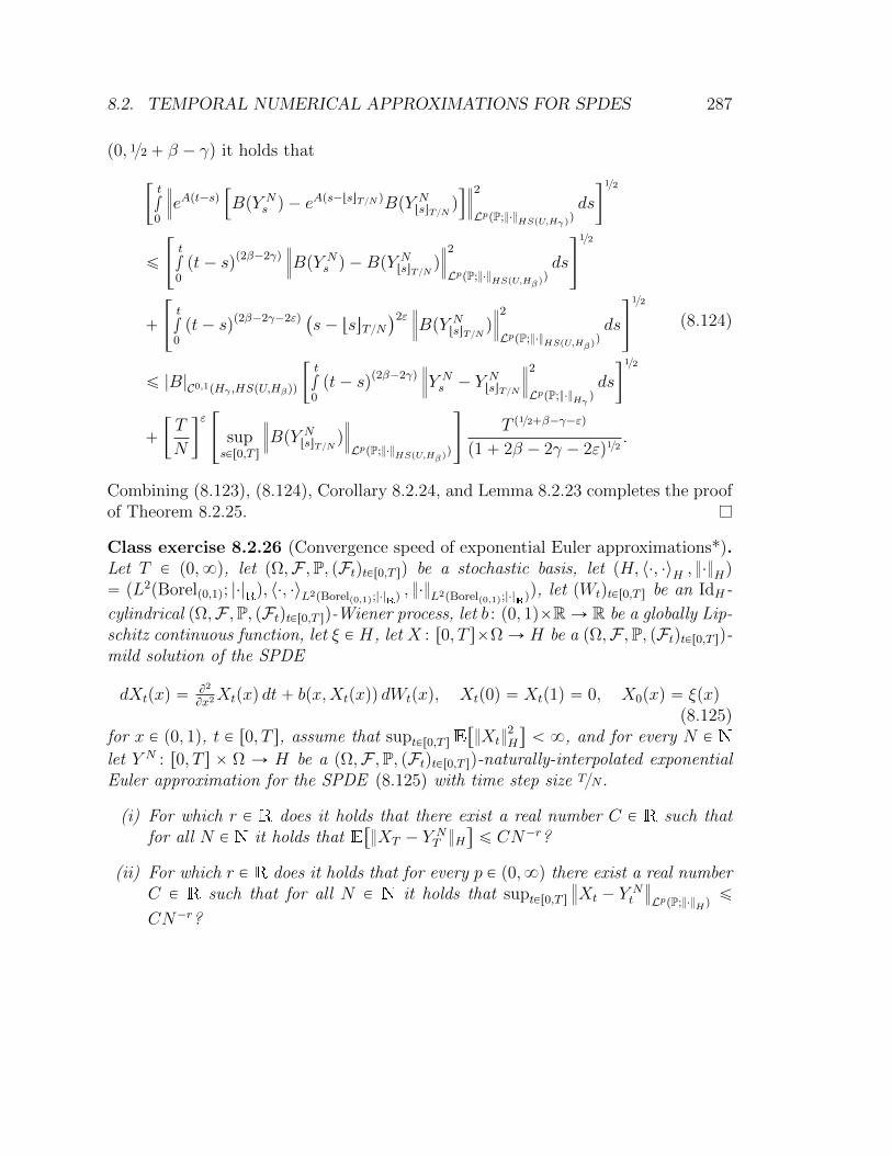
8.2. TEMPORAL NUMERICAL APPROXIMATIONS FOR SPDES 287
p0, 12` β ´ γq it holds that
„
t
∫0
›
›
›eApt´sq
”
BpY Ns q ´ e
Aps´tsuT N qBpY NtsuT N
q
ı›
›
›
2
LppP;¨HSpU,Hγ qqds
12
ď
«
t
∫0pt´ sqp2β´2γq
›
›
›BpY N
s q ´BpYN
tsuT Nq
›
›
›
2
LppP;¨HSpU,Hβqqds
ff12
`
«
t
∫0pt´ sqp2β´2γ´2εq
`
s´ tsuT N˘2ε
›
›
›BpY N
tsuT Nq
›
›
›
2
LppP;¨HSpU,Hβqqds
ff12
ď |B|C0,1pHγ ,HSpU,Hβqq
„
t
∫0pt´ sqp2β´2γq
›
›
›Y Ns ´ Y N
tsuT N
›
›
›
2
LppP;¨Hγ qds
12
`
„
T
N
ε«
supsPr0,T s
›
›
›BpY N
tsuT Nq
›
›
›
LppP;¨HSpU,Hβqq
ff
T p12`β´γ´εq
p1` 2β ´ 2γ ´ 2εq12.
(8.124)
Combining (8.123), (8.124), Corollary 8.2.24, and Lemma 8.2.23 completes the proofof Theorem 8.2.25.
Class exercise 8.2.26 (Convergence speed of exponential Euler approximations*).Let T P p0,8q, let pΩ,F ,P, pFtqtPr0,T sq be a stochastic basis, let pH, 〈¨, ¨〉H , ¨Hq“ pL2pBorelp0,1q; |¨|Rq, 〈¨, ¨〉L2pBorelp0,1q;|¨|Rq
, ¨L2pBorelp0,1q;|¨|Rqq, let pWtqtPr0,T s be an IdH-
cylindrical pΩ,F ,P, pFtqtPr0,T sq-Wiener process, let b : p0, 1qˆRÑ R be a globally Lip-schitz continuous function, let ξ P H, let X : r0, T sˆΩ Ñ H be a pΩ,F ,P, pFtqtPr0,T sq-mild solution of the SPDE
dXtpxq “B2
Bx2Xtpxq dt` bpx,Xtpxqq dWtpxq, Xtp0q “ Xtp1q “ 0, X0pxq “ ξpxq
(8.125)for x P p0, 1q, t P r0, T s, assume that suptPr0,T sE
“
Xt2H
‰
ă 8, and for every N P N
let Y N : r0, T s ˆ Ω Ñ H be a pΩ,F ,P, pFtqtPr0,T sq-naturally-interpolated exponentialEuler approximation for the SPDE (8.125) with time step size TN.
(i) For which r P R does it holds that there exist a real number C P R such thatfor all N P N it holds that E
“
XT ´ YNT H
‰
ď CN´r?
(ii) For which r P R does it holds that for every p P p0,8q there exist a real numberC P R such that for all N P N it holds that suptPr0,T s
›
›Xt ´ YNt
›
›
LppP;¨Hqď
CN´r?

288 CHAPTER 8. STRONG NUMERICAL APPROXIMATIONS FOR SPDES
8.3 Noise approximations for SPDEs
8.3.1 Noise perturbation estimates
The next result, Corollary 8.3.1, is an immediate consequence of Proposition 7.1.6,Theorem 4.8.5, and Theorem 6.3.29.
Corollary 8.3.1 (Noise perturbation). Assume the setting in Section 7.1.2, let θ Prγ ´ β, 12q, B P C0,1pHγ, HSpU,Hβqq, and let X, X : r0, T s ˆ Ω Ñ Hγ be stochasticprocesses which satisfy supsPr0,T s
“
XsLppP;¨Hγ q` XsLppP;¨Hγ q
‰
ă 8, which satisfy
that X is a pΩ,F ,P, pFtqtPr0,T sq-mild solution of the SPDE
dXt “ rAXt ` F pXtqs dt`BpXtq dWt, t P r0, T s, X0 “ ξ, (8.126)
and which satisfy that X is a pΩ,F ,P, pFtqtPr0,T sq-mild solution of the SPDE
dXt ““
AXt ` F pXtq‰
dt` BpXtq dWt, t P r0, T s, X0 “ ξ. (8.127)
Then
suptPr0,T s
›
›Xt ´ Xt
›
›
LppP;¨Hγ q
ď Ep1´ηq„
T 1´η?
2 |F |C0,1pHγ,Hγ´ηq?1´η
`a
T 1´ηppp´ 1q |B|C0,1pHγ ,HSpU,Hγ´η2qq
¨T p12´θq
a
p pp´ 1q?
1´ 2θ
«
suptPp0,T q
›
›BpXsq ´ BpXsq›
›
LppP;¨HSpU,Hγ´θqq
ff
ă 8.
(8.128)
Proof. Proposition 7.1.6 ensures that
suptPr0,T s
›
›X1t ´X
2t
›
›
LppP;¨Hγ q
ď Ep1´ηq„
T 1´η?
2 |F |C0,1pHγ,Hγ´ηq?1´η
`a
T 1´ηppp´ 1q |B|C0,1pHγ ,HSpU,Hγ´η2qq
¨?
2 suptPr0,T s
›
›
›
›
„
Xt ´
ż t
0
eApt´sqF pXsq ds´
ż t
0
eApt´sqBpXsq dWs
`
„ż t
0
eApt´sqF pXsq ds`
ż t
0
eApt´sqBpXsq dWs ´ Xt
›
›
›
›
LppP;¨Hγ q
ă 8.
(8.129)

8.3. NOISE APPROXIMATIONS FOR SPDES 289
This implies that
suptPr0,T s
›
›X1t ´X
2t
›
›
LppP;¨Hγ q
ď Ep1´ηq„
T 1´η?
2 |F |C0,1pHγ,Hγ´ηq?1´η
`a
T 1´ηppp´ 1q |B|C0,1pHγ ,HSpU,Hγ´η2qq
¨?
2 suptPr0,T s
›
›
›
›
ż t
0
eApt´sq“
BpXsq ´ BpXsq‰
dWs
›
›
›
›
LppP;¨Hγ q
ă 8.
(8.130)
Theorem 6.3.29. and Theorem 4.8.5 hence prove that
suptPr0,T s
›
›X1t ´X
2t
›
›
LppP;¨Hγ q
ď Ep1´ηq„
T 1´η?
2 |F |C0,1pHγ,Hγ´ηq?1´η
`a
T 1´ηppp´ 1q |B|C0,1pHγ ,HSpU,Hγ´η2qq
¨?
2
«
p pp´1q2
suptPr0,T s
ż t
0
s´2θds
ff12 «
supsPp0,T q
›
›BpXsq ´ BpXsq›
›
LppP;¨HSpU,Hγ´θqq
ff
ă 8.
(8.131)
This completes the proof of Corollary 8.3.1.
8.3.2 Noise approximations for SPDEs
The next result, Corollary 8.3.2, is an immediate consequence from Corollary 8.3.1above.
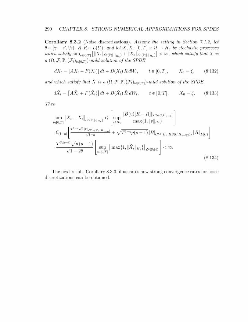
290 CHAPTER 8. STRONG NUMERICAL APPROXIMATIONS FOR SPDES
Corollary 8.3.2 (Noise discretizations). Assume the setting in Section 7.1.2, letθ P rγ ´ β, 12q, R, R P LpUq, and let X, X : r0, T s ˆ Ω Ñ Hγ be stochastic processeswhich satisfy supsPr0,T s
“
XsLppP;¨Hγ q` XsLppP;¨Hγ q
‰
ă 8, which satisfy that X is
a pΩ,F ,P, pFtqtPr0,T sq-mild solution of the SPDE
dXt “ rAXt ` F pXtqs dt`BpXtqRdWt, t P r0, T s, X0 “ ξ, (8.132)
and which satisfy that X is a pΩ,F ,P, pFtqtPr0,T sq-mild solution of the SPDE
dXt ““
AXt ` F pXtq‰
dt`BpXtq R dWt, t P r0, T s, X0 “ ξ. (8.133)
Then
suptPr0,T s
›
›Xt ´ Xt
›
›
LppP;¨Hγ qď
«
supvPHγ
BpvqrR ´ RsHSpU,Hγ´θq
maxt1, vHγu
ff
¨ Ep1´ηq„
T 1´η?
2 |F |C0,1pHγ,Hγ´ηq?1´η
`a
T 1´ηppp´ 1q |B|C0,1pHγ ,HSpU,Hγ´η2qqRLpUq
¨T p12´θq
a
p pp´ 1q?
1´ 2θ
«
suptPr0,T s
›
›maxt1, XsHγu›
›
LppP;|¨|q
ff
ă 8.
(8.134)
The next result, Corollary 8.3.3, illustrates how strong convergence rates for noisediscretizations can be obtained.

8.3. NOISE APPROXIMATIONS FOR SPDES 291
Corollary 8.3.3. Assume the setting in Section 7.1.2, let θ P rγ ´ β, 12q, r P
r0,8q, pRNqNPN0 Ď LpUq satisfy supNPN supvPHγNrBpvqrR0´RN sHSpU,Hγ´θq
maxt1,vHγ uă 8, and
let XN : r0, T s ˆ Ω Ñ Hγ, N P N0, be stochastic processes with the property that@N P N0 : supsPr0,T s XsLppP;¨Hγ q
ă 8 and with the property that for all N P N0 it
holds that XN is a pΩ,F ,P, pFtqtPr0,T sq-mild solution of the SPDE
dXNt “
“
AXNt ` F pX
Nt q
‰
dt`BpXNt qRN dWt, t P r0, T s, X0 “ ξ. (8.135)
Then
suptPr0,T s
›
›X0t ´X
Nt
›
›
LppP;¨Hγ qď
1
N r
«
supMPN
supvPHγ
M rBpvqrR0 ´RM sHSpU,Hγ´θq
maxt1, vHγu
ff
¨ Ep1´ηq„
T 1´η?
2 |F |C0,1pHγ,Hγ´ηq?1´η
`a
T 1´ηppp´ 1q |B|C0,1pHγ ,HSpU,Hγ´η2qqR0LpUq
¨T p12´θq
a
p pp´ 1q?
1´ 2θ
«
suptPr0,T s
supMPN
›
›maxt1, XMs Hγu
›
›
LppP;|¨|q
ff
ă 8.
(8.136)
Proof of Corollary 8.3.3. First, observe that Proposition 7.1.15 ensures that for allM P N0 it holds that
suptPr0,T s
›
›max
1, XMt Hγ
(›
›
LppP;|¨|qď?
2›
›max
1, ξHγ(›
›
LppP;|¨|q
¨ Ep1´ηq„
T 1´η?
2 F LGpHγ,Hγ´ηq?1´η
`a
T 1´ηppp´ 1q Bp¨qRMLGpHγ ,HSpU,Hγ´η2qq
ă 8.
(8.137)
Next note that the assumption that supNPN supvPHγNrBpvqrR0´RN sHSpU,Hγ´θq
maxt1,vHγ uă 8
implies that
supMPN0
Bp¨qRMLGpHγ ,HSpU,Hγ´η2qq“ sup
MPN0
supvPHγ
«
BpvqRMHSpU,Hγ´η2q
max
1, vHγ(
ff
ď supvPHγ
«
BpvqHSpU,Hγ´η2qR0LpUq
max
1, vHγ(
ff
` supMPN0
supvPHγ
«
BpvqrR0 ´RM sHSpU,Hγ´η2q
max
1, vHγ(
ff
ă 8.
(8.138)

292 CHAPTER 8. STRONG NUMERICAL APPROXIMATIONS FOR SPDES
This and (8.137) prove that
supMPN0
suptPr0,T s
›
›max
1, XMt Hγ
(›
›
LppP;|¨|qă 8. (8.139)
This and Corollary 8.3.2 complete the proof of Corollary 8.3.3.
8.4 Full discretizations for SPDEs
8.4.1 Setting
Assume the setting in Section 7.1.2, let B Ď H be an orthonormal basis of H, letU Ď U be an orthonormal basis of U , let λ : B Ñ R be a function, assume thatDpAq “
v P H :ř
bPB |λb 〈b, v〉H |2ă 8
(
, assume that for all v P DpAq it holds thatAv “
ř
bPB λb 〈b, v〉H b and let pπIqIPPpBq Ď LpHγ´ηq and p$IqIPPpUq Ď LpUq satisfythat for all v P Hγ´η, u P U , I P PpBq, J P PpUq it holds that
πIpvq “ÿ
bPI
〈b, v〉H b and $Jpuq “ÿ
bPJ
〈b, u〉U b. (8.140)
8.4.2 Full-discrete spectral Galerkin exponential Euler methodfor SPDEs
Definition 8.4.1 (Full discrete spectral Galerkin exponential Euler approxima-tions). Assume the setting in Section 8.4.1, let N P N, I P PpBq, J P PpUq andlet Y : t0, 1, . . . , Nu ˆ Ω Ñ πIpHγq be a pFnTNqnPt0,1,...,Nu/BpHγq-adapted stochasticprocess which fulfills Y0 “ πIpξq and which fulfills that for all n P t0, 1, . . . , N ´ 1u itholds P-a.s. that
Yn`1 “ eATN
˜
Yn ` πIpF pYnqqTN`
ż pn`1qTN
nTN
πI`
BpYnq$JpdWsq˘
¸
. (8.141)
Then we call Y a full-discrete spectral Galerkin exponential Euler approximation forthe SPDE
dXt “ rAXt ` F pXtqs dt`BpXtq dWt, t P r0, T s, X0 “ ξ (8.142)
with time step size TN, spatial approximation I and noise approximation J .

8.4. FULL DISCRETIZATIONS FOR SPDES 293
1 function Y = ExpEuler (T, v , f , b , xi ,N,M)2 A = ´v∗pi ˆ2∗ (1 :M) . ˆ 2 ; Y = i d s t ( x i ) / sqrt ( 2 ) ;3 for n=1:N4 y = dst (Y) ∗ sqrt ( 2 ) ;5 dW = dst ( randn (1 ,M) .∗ sqrt (2∗T/N) ) ;6 y = y + f ( y )∗T/N + b( y ) . ∗dW;7 Y = exp( A∗T/N ) .∗ i d s t ( y ) / sqrt ( 2 ) ;8 end9 Y = [ 0 , dst (Y)∗ sqrt ( 2 ) , 0 ] ;
10 end
Matlab code 8.1: A Matlab function for simulating a full-discrete spectralGalerkin exponential Euler approximation for the SPDE (7.78).
1 clear a l l2 rng ( ’ d e f a u l t ’ )3 T = 1 ; v = 1/50 ; M = 2ˆ8´1; N = Mˆ2 ;4 f = @( x ) 1´x ; b = @( x ) (1´x )./(1+ x . ˆ 2 ) / 4 ;5 x i = zeros (1 ,M) ;6 Preimage = ( 0 :M+1)/(M+1);7 hold on8 Y = ExpEuler (T, v , f , b , xi ,N,M) ;9 plot ( Preimage ,Y) ;
10 Y = ExpEuler (T, v , f , b , xi ,N,M) ;11 plot ( Preimage ,Y, ’ r ’ ) ;12 Y = ExpEuler (T, v , f , b , xi ,N,M) ;13 plot ( Preimage ,Y, ’ g ’ ) ;14 hold o f f
Matlab code 8.2: A Matlab code for simulating a full-discrete spectral Galerkinexponential Euler approximation for an SPDE of the form (7.78).

294 CHAPTER 8. STRONG NUMERICAL APPROXIMATIONS FOR SPDES
0 0.1 0.2 0.3 0.4 0.5 0.6 0.7 0.8 0.9 1−0.4
−0.2
0
0.2
0.4
0.6
0.8
1
Figure 8.1: Result of a call of the Matlab code 8.2.

8.4. FULL DISCRETIZATIONS FOR SPDES 295
8.4.3 Full-discrete spectral Galerkin linear-implicit Euler methodfor SPDEs
Definition 8.4.2 (Full-discrete spectral Galerkin linear-implicit Euler approxima-tions). Assume the setting in Section 8.4.1, let N P N, I P PpBq, J P PpUq, andlet Y : t0, 1, . . . , Nu ˆ Ω Ñ πIpHγq be a pFnTNqnPt0,1,...,Nu/BpHγq-adapted stochasticprocess which fulfills Y0 “ πIpξq and which fulfills that for all n P t0, 1, . . . , N ´ 1u itholds P-a.s. that
Yn`1 “`
IdH ´TNA˘´1
˜
Yn ` πI`
F pYnq˘
TN`
ż pn`1qTN
nTN
πI`
BpYnq$JpdWsq˘
¸
.
(8.143)
Then we call Y a full-discrete spectral Galerkin linear-implicit Euler approximationfor the SPDE
dXt “ rAXt ` F pXtqs dt`BpXtq dWt, t P r0, T s, X0 “ ξ (8.144)
with time step size TN, spatial approximation I and noise approximation J .
1 function Y = LinImpEuler (T, v , f , b , xi ,N,M)2 A = ´v∗pi ˆ2∗ (1 :M) . ˆ 2 ; Y = i d s t ( x i ) / sqrt ( 2 ) ;3 for n=1:N4 y = dst (Y) ∗ sqrt ( 2 ) ;5 dW = dst ( randn (1 ,M) .∗ sqrt (2∗T/N) ) ;6 y = y + f ( y )∗T/N + b( y ) . ∗dW;7 Y = i d s t ( y ) / sqrt (2 ) . / ( 1 ´ A∗T/N ) ;8 end9 Y = [ 0 , dst (Y)∗ sqrt ( 2 ) , 0 ] ;
10 end
Matlab code 8.3: A Matlab function for simulating a full-discrete spectralGalerkin linear-implicit Euler approximation of the SPDE (7.78).
1 clear a l l2 rng ( ’ d e f a u l t ’ )3 T = 1 ; v = 1/50 ; M = 2ˆ8´1; N = Mˆ2 ;4 f = @( x ) 1´x ; b = @( x ) (1´x )./(1+ x . ˆ 2 ) / 4 ;5 x i = zeros (1 ,M) ;

296 CHAPTER 8. STRONG NUMERICAL APPROXIMATIONS FOR SPDES
6 Preimage = ( 0 :M+1)/(M+1);7 hold on8 Y = LinImpEuler (T, v , f , b , xi ,N,M)9 plot ( Preimage ,Y) ;
10 Y = LinImpEuler (T, v , f , b , xi ,N,M)11 plot ( Preimage ,Y, ’ r ’ ) ;12 Y = LinImpEuler (T, v , f , b , xi ,N,M)13 plot ( Preimage ,Y, ’ g ’ ) ;14 hold o f f
Matlab code 8.4: A Matlab code for simulating a full-discrete spectral Galerkinlinear-implicit Euler approximation of the SPDE (7.78).
0 0.1 0.2 0.3 0.4 0.5 0.6 0.7 0.8 0.9 1−0.4
−0.2
0
0.2
0.4
0.6
0.8
1
Figure 8.2: Result of a call of the Matlab code 8.4.

8.4. FULL DISCRETIZATIONS FOR SPDES 297
8.4.4 Full-discrete spectral Galerkin nonlinearity-stopped ex-ponential Euler method for SPDEs
Definition 8.4.3 (Full-discrete spectral Galerkin nonlinearity-stopped exponentialEuler approximations). Assume the setting in Section 8.4.1, let N P N, I P PpBq, J PPpUq, α P rγ´η, γs, assume that F pHγq Ď Hα and let Y : t0, 1, . . . , NuˆΩ Ñ πIpHγq
be a pFnTNqnPt0,1,...,Nu/BpHγq-adapted stochastic process which fulfills Y0 “ πIpξq andwhich fulfills that for all n P t0, 1, . . . , N ´ 1u it holds P-a.s. that
Yn`1 “ 1tπIpF pYnqq2HαąNTuYn (8.145)
` 1tπIpF pYnqq2HαďNTueA
TN
˜
Yn ` πI`
F pYnq˘
TN`
ż pn`1qTN
nTN
πI`
BpYnq$JpdWsq˘
¸
.
Then we call Y a full-discrete spectral Galerkin nonlinearity-stopped exponential Eu-ler approximation for the SPDE
dXt “ rAXt ` F pXtqs dt`BpXtq dWt, t P r0, T s, X0 “ ξ (8.146)
with time step size TN, spatial approximation I and noise approximation J .
1 function Y = StopExpEuler (T, v , f , b , xi ,N,M)2 A = ´v∗pi ˆ2∗ (1 :M) . ˆ 2 ; Y = i d s t ( x i ) / sqrt ( 2 ) ;3 for n=1:N4 y = dst (Y) ∗ sqrt ( 2 ) ;5 z = f ( y ) ;6 i f ( sum( i d s t ( z ) . ˆ 2 ) > 2∗N/T ) break ; end7 dW = dst ( randn (1 ,M) .∗ sqrt (2∗T/N) ) ;8 y = y + z∗T/N + b( y ) . ∗dW;9 Y = exp( A∗T/N ) .∗ i d s t ( y ) / sqrt ( 2 ) ;
10 end11 Y = [ 0 , dst (Y)∗ sqrt ( 2 ) , 0 ] ;12 end
Matlab code 8.5: A Matlab function for simulating a full-discrete spectralGalerkin nonlinearity-stopped exponential Euler approximation for a generalized ver-sion of the SPDE (7.78) with γ P p1
5, 1
4q and α “ 0.
1 clear a l l2 rng ( ’ d e f a u l t ’ )

298 CHAPTER 8. STRONG NUMERICAL APPROXIMATIONS FOR SPDES
3 T = 1 ; v = 1/50 ; M = 2ˆ8´1; N = Mˆ2 ;4 f = @( x ) 1´x . ˆ 3 ; b = @( x ) x /4 ;5 x i = zeros (1 ,M) ;6 Preimage = ( 0 :M+1)/(M+1);7 hold on8 Y = StopExpEuler (T, v , f , b , xi ,N,M) ;9 plot ( Preimage ,Y) ;
10 Y = StopExpEuler (T, v , f , b , xi ,N,M) ;11 plot ( Preimage ,Y, ’ r ’ ) ;12 Y = StopExpEuler (T, v , f , b , xi ,N,M) ;13 plot ( Preimage ,Y, ’ g ’ ) ;14 hold o f f
Matlab code 8.6: A Matlab code for simulating a full-discrete spectral Galerkinnonlinearity-stopped exponential Euler approximation for a generalized version ofthe SPDE (7.78) with γ P p1
5, 1
4q and α “ 0.
8.4.5 Full-discrete spectral Galerkin nonlinearity-stopped linear-implicit Euler method for SPDEs
Definition 8.4.4 (Full-discrete spectral Galerkin nonlinearity-stopped linear-im-plicit Euler approximations). Assume the setting in Section 8.4.1, let N P N, I PPpHq, J P PpUq, α P rγ´ η, γs, assume that F pHγq Ď Hα and let Y : t0, 1, . . . , NuˆΩ Ñ πIpHγq be a pFnTNqnPt0,1,...,Nu/BpHγq-adapted stochastic process which fulfillsY0 “ πIpξq and which fulfills that for all n P t0, 1, . . . , N ´ 1u it holds P-a.s. that
Yn`1 “ 1tπIpF pYnqq2HαąNTuYn (8.147)
` 1tπIpF pYnqq2HαďNTu
`
IdH ´TNA˘´1
˜
Yn ` πI`
F`
Yn˘˘
TN`
ż pn`1qTN
nTN
πI`
BpYnq$JpdWsq˘
¸
.
Then we call Y a spectral Galerkin nonlinearity-stopped linear-implicit Euler approx-imation for the SPDE
dXt “ rAXt ` F pXtqs dt`BpXtq dWt, t P r0, T s, X0 “ ξ (8.148)
with time step size TN, spatial approximation I and noise approximation J .

8.4. FULL DISCRETIZATIONS FOR SPDES 299
0 0.1 0.2 0.3 0.4 0.5 0.6 0.7 0.8 0.9 10
0.2
0.4
0.6
0.8
1
1.2
1.4
Figure 8.3: Result of a call of the Matlab code 8.6.

300 CHAPTER 8. STRONG NUMERICAL APPROXIMATIONS FOR SPDES
1 function Y = StopLinImpEuler (T, v , f , b , xi ,N,M)2 A = ´v∗pi ˆ2∗ (1 :M) . ˆ 2 ; Y = i d s t ( x i ) / sqrt ( 2 ) ;3 for n=1:N4 y = dst (Y) ∗ sqrt ( 2 ) ;5 z = f ( y ) ;6 i f ( sum( i d s t ( z ) . ˆ 2 ) > 2∗N/T ) break ; end7 dW = dst ( randn (1 ,M) .∗ sqrt (2∗T/N) ) ;8 y = y + z∗T/N + b( y ) . ∗dW;9 Y = i d s t ( y ) / sqrt (2 ) . / ( 1 ´ A∗T/N ) ;
10 end11 Y = [ 0 , dst (Y)∗ sqrt ( 2 ) , 0 ] ;12 end
Matlab code 8.7: A Matlab function for simulating a full-discrete spectralGalerkin nonlinearity-stopped linear-implicit Euler approximation for a generalizedversion of the SPDE (7.78) with γ P p1
5, 1
4q and α “ 0.
1 clear a l l2 rng ( ’ d e f a u l t ’ )3 T = 1 ; v = 1/50 ; M = 2ˆ8´1; N = Mˆ2 ;4 f = @( x ) 1´x . ˆ 3 ; b = @( x ) x /4 ;5 x i = zeros (1 ,M) ;6 Preimage = ( 0 :M+1)/(M+1);7 hold on8 Y = StopLinImpEuler (T, v , f , b , xi ,N,M) ;9 plot ( Preimage ,Y) ;
10 Y = StopLinImpEuler (T, v , f , b , xi ,N,M) ;11 plot ( Preimage ,Y, ’ r ’ ) ;12 Y = StopLinImpEuler (T, v , f , b , xi ,N,M) ;13 plot ( Preimage ,Y, ’ g ’ ) ;14 hold o f f
Matlab code 8.8: A Matlab code for simulating a spectral Galerkin nonlinearity-stopped linear-implicit Euler approximation for a generalized version of theSPDE (7.78) with γ P p1
5, 1
4q and α “ 0.

8.4. FULL DISCRETIZATIONS FOR SPDES 301
0 0.1 0.2 0.3 0.4 0.5 0.6 0.7 0.8 0.9 10
0.2
0.4
0.6
0.8
1
1.2
1.4
Figure 8.4: Result of a call of the Matlab code 8.8.

302 CHAPTER 8. STRONG NUMERICAL APPROXIMATIONS FOR SPDES

Chapter 9
Solutions to selected exercises
9.1 Chapter 2
9.1.1 Solution to Exercise 2.2.6
Lemma 9.1.1. Let pΩ,Fq be a measurable space, let pE, dEq be a metric space, andlet f : Ω Ñ E be a function. Then f is F/BpEq-measurable if and only if it holdsfor all ϕ P CpE,Rq that ϕ ˝ f is F/BpRq-measurable.
Proof of Lemma 9.1.1. First of all, recall that every ϕ P CpE,Rq is BpEq/BpRq-measurable. This shows that f PMpF ,BpEqq implies that for every ϕ P CpE,Rq itholds that the composition ϕ ˝ f is F/BpRq-measurable. It thus remains to provethat @ϕ P CpE,Rq : ϕ ˝ f P MpF ,BpRqq ensures that f is F/BpEq-measurable.This, in turn, is an immediate consequence from Proposition 2.2.5. The proof ofLemma 9.1.1 is thus completed.
303

304 CHAPTER 9. SOLUTIONS TO SELECTED EXERCISES

Bibliography
[1] Cohn, D. L. Measure theory. Birkhauser Boston Inc., Boston, MA, 1993.Reprint of the 1980 original.
[2] Cox, S., Hutzenthaler, M., Jentzen, A., van Neerven, J., andWelti, T. Convergence in the holder norm with applications to monte carlomethods in infinite dimensions. Unpublished manuscript, 2014.
[3] Da Prato, G., and Zabczyk, J. Stochastic equations in infinite dimen-sions, vol. 44 of Encyclopedia of Mathematics and its Applications. CambridgeUniversity Press, Cambridge, 1992.
[4] Hardy, G. H., Littlewood, J. E., and Polya, G. Inequalities. CambridgeMathematical Library. Cambridge University Press, Cambridge, 1988. Reprintof the 1952 edition.
[5] Henry, D. Geometric theory of semilinear parabolic equations, vol. 840 ofLecture Notes in Mathematics. Springer-Verlag, Berlin, 1981. 348 pages.
[6] Heuser, H. Lehrbuch der Analysis. Teil 2, sixth ed. Mathematische Leitfaden.[Mathematical Textbooks]. B. G. Teubner, Stuttgart, 1991.
[7] Heuser, H. Lehrbuch der Analysis. Teil 1, fifteenth ed. MathematischeLeitfaden. [Mathematical Textbooks]. B. G. Teubner, Stuttgart, 2003.
[8] Hutzenthaler, M., Jentzen, A., and Kloeden, P. E. Divergence ofthe multilevel Monte Carlo Euler method for nonlinear stochastic differentialequations. To appear in Ann. Appl. Probab. (2013); arXiv:1105.0226 (2011),31 pages.
[9] Hutzenthaler, M., Jentzen, A., and Kloeden, P. E. Strong and weakdivergence in finite time of Euler’s method for stochastic differential equations
305
306 BIBLIOGRAPHY
with non-globally Lipschitz continuous coefficients. Proc. R. Soc. Lond. Ser. AMath. Phys. Eng. Sci. 467 (2011), 1563–1576.
[10] Jentzen, A., and Kloeden, P. Taylor Approximations for Stochastic PartialDifferential Equations, vol. 83 of CBMS-NSF Regional Conference Series inApplied Mathematics. Society for Industrial and Applied Mathematics (SIAM),Philadelphia, PA, 2012.
[11] Jentzen, A., and Kurniawan, R. Weak convergence rates for Euler-typeapproximations of semilinear stochastic evolution equations with nonlinear dif-fusion coefficients. arXiv:1501.03539 (2015), 1–51.
[12] Karatzas, I., and Shreve, S. E. Brownian motion and stochastic calculus,second ed., vol. 113 of Graduate Texts in Mathematics. Springer-Verlag, NewYork, 1991.
[13] Klenke, A. Probability theory. Universitext. Springer-Verlag London Ltd.,London, 2008. A comprehensive course, Translated from the 2006 German orig-inal.
[14] Klenke, A. Probability theory. Universitext. Springer-Verlag London Ltd.,London, 2008. A comprehensive course, Translated from the 2006 German orig-inal.
[15] Kuhn, C. Stochastische Analysis mit Finanzmathematik. 2004.
[16] Kurniawan, R. Numerical approximations of stochastic partial differentialequations with non-globally Lipschitz continuous nonlinearities. University ofZurich and ETH Zurich, Zurich, Switzerland, 2014. 74 pages. Master thesis.
[17] Pazy, A. Semigroups of linear operators and applications to partial differentialequations, vol. 44 of Applied Mathematical Sciences. Springer-Verlag, New York,1983.
[18] Prevot, C., and Rockner, M. A concise course on stochastic partial dif-ferential equations, vol. 1905 of Lecture Notes in Mathematics. Springer, Berlin,2007. 144 pages.
[19] Reed, M., and Simon, B. Methods of modern mathematical physics. I. Func-tional analysis. Academic Press, New York, 1972.

BIBLIOGRAPHY 307
[20] Stein, E. M. Singular integrals and differentiability properties of functions.Princeton Mathematical Series, No. 30. Princeton University Press, Princeton,N.J., 1970.
[21] Van Neerven, J. Stochastic Evolution Equations. Lec-ture notes (2007), 234 pages. Available online athttp://fa.its.tudelft.nl/„neerven/publications/papers/ISEM.pdf.
[22] van Neerven, J. M. A. M., Veraar, M. C., and Weis, L. Stochasticevolution equations in UMD Banach spaces. J. Funct. Anal. 255, 4 (2008),940–993.
[23] Werner, D. Funktionalanalysis, extended ed. Springer-Verlag, Berlin, 2005.


![A Minicourse on Stochastic Partial Di erential Equations13] Guisseppe Da Prato and Jerzy Zabczyk (1992). Stochastic Equations in In nite Dimensions, Encyclopedia of Mathematics and](https://cdn.vdocuments.site/doc/165x107/5ed5eb4fc46614170c62b9bb/a-minicourse-on-stochastic-partial-di-erential-equations-13-guisseppe-da-prato.jpg)


