
Statistical Learning Theory: Classification Using Support Vector MachinesJohn DiMona
Some slides based onProf Andrew Moore at CMU: http://www.cs.cmu.edu/~awm/tutorials

(Rough) Outline1. Empirical Modeling2. Risk Minimization
i. Theoryii. Empirical Risk Minimizationiii. Structural Risk Minimization
3. Optimal Separating Hyperplanes4. Support Vector Machines5. Example6. Questions

Empirical Data Modeling
• Observations of a system are collected• Based on these observations a process of
induction is used to build up a model of the system
• This model is used to deduce responses of the system not yet observed

Empirical Data Modeling
• Data obtained through observation is finite and sampled by nature
• Typically this sampling is non-uniform• Due to the high dimensional nature of some
problems the data will form only a sparse distribution in the input space
• Creating a model from this type of data is an ill posed problem

Empirical Data Modeling
The goal in modeling is to choose a model from the hypothesis space, which is closest (with respect to some error measure) to the
underlying function in the target space.
Globally Optimal Model
Best Reachable ModelSelected Model

Error in Modeling
• Approximation Error is a consequence of the hypothesis space not exactly fitting target space, – The underlying function may lie outside the
hypothesis space– A poor choice of the model space will result in a large
approximation error (model mismatch)
• Estimation Error is the error due to the learning procedure converging to a non-optimal model in the hypothesis space
• Together these form the Generalization Error

Error in Modeling
The goal in modeling is to choose a model from the hypothesis space, which is closest (with respect to some error measure) to the
underlying function in the target space.
Globally Optimal Model
Best Reachable ModelSelected Model

Pattern Recognition
• Given a system , where:
• Develop a model , that best predicts the behavior of the system for all possible items .
Y (x) y
x (x1, ... , x n ) X Rn
and
y { 1, 1}
The item we want to classify
The true classification of that item
f (x) ˆ y
x X

Supervised Learning
i. A generator (G) of a set of vectors , observed independently from the system with a fixed, unknown probability distribution
ii. A supervisor (S) who returns an output value to every input vector , according to the systems conditional probability function (also unknown)
iii. A learning machine (LM) capable of implementing a set of functions , where is a set of parameters
x Rn
P(x)
y
x
P(y | x)
f (x,),
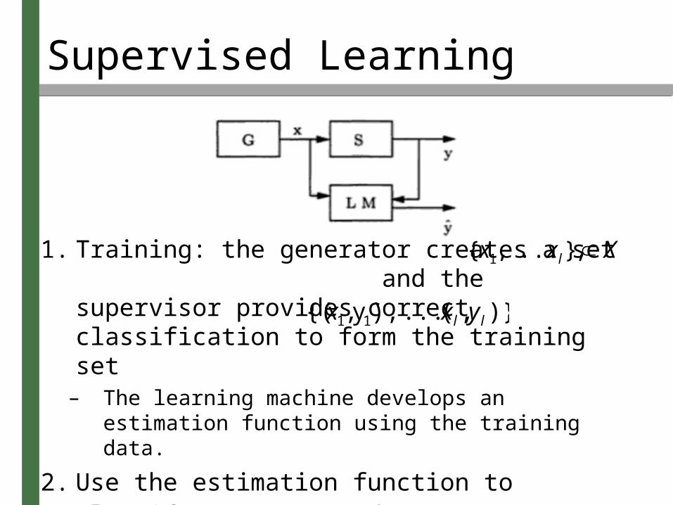
Supervised Learning
1. Training: the generator creates a set and the supervisor provides correct classification to form the training set
– The learning machine develops an estimation function using the training data.
2. Use the estimation function to classify new unseen data
{x1, ... , x l} X
{(x1,y1), ... , (x l , y l )}

Risk Minimization
• In order to choose the best estimation function we must have a measure of discrepancy between a true classification of
and an estimated classification
For pattern recognition we use:
x
Y (x) y
f (x,) ˆ y
L(y, f (x,)) 0 if y f (x,)
1 if y f (x,)

Risk Minimization
• The expected value of loss with regards to some estimation function :
where
f (x,)
R() L(y, f (x,))d P(x,y)
P(x,y) P(x)P(y | x)

Risk Minimization
• The expected value of loss with regards to some estimation function :
where
• Goal: Find the function that minimizes the risk (over all functions )
f (x,)
R() L(y, f (x,))d P(x,y)
P(x,y) P(x)P(y | x)
f (x,0)
R()
f (x,),

Risk Minimization
• The expected value of loss with regards to some estimation function :
where
• Goal: Find the function that minimizes the risk (over all functions )
• Problem: By definition we don’t know
f (x,)
R() L(y, f (x,))d P(x,y)
P(x,y) P(x)P(y | x)
f (x,0)
R()
P(x, y)
f (x,),

To make things clearer…
• The training set will be referred to as
• The loss function will be
{(x1,y1), ... , (x l , y l )}
{z1, ... ,zl}
L(y, f (x,))
Q(z,)
For the coming discussion we will shorten notation in the following ways

Empirical Risk Minimization (ERM)
• Instead of measuring risk over the set of all just measure it over just the training set
• The empirical risk must converge uniformly to the actual risk over the set of loss functions in both directions:
Xx
{z1, ... ,zl}
l
iizQ
lR
1emp ,(
1(
(empR
(R
,,(zQ
((lim emp RRl
(min(minlim emp RRl

VC Dimension (Vapnik–Chervonenkis Dimension)
• The VC dimension is a scalar value that measures the capacity of a set of functions.
• The VC dimension of a set of functions is if and only if there exists a set of points such that these points can be separated in all
h
possible configurations, and that no set exists where satisfying this property.
h2
{x i}i1h
{x i}i1q hq

VC Dimension (Vapnik–Chervonenkis Dimension)
•Three points in the plane can be shattered by the set of linear indicator functions whereas four points cannot
•The set of linear indicator functions in n dimensional space has a VC dimension equal to n + 1

Upper Bound for Risk
• It can be shown that ,where is the confidence interval and is the VC dimension
• ERM only minimizes , and , the confidence interval, is fixed based on the VC dimension of the set of functions determined a priori
• When implementing ERM one must tune the confidence interval based on the problem to avoid underfitting/overfitting the data
h
l
R( l ) Remp( l ) l
h
h
)(emp lR
h
l
),(y,αf

Structural Risk Minimization (SRM)
• SRM attempts to minimize the right hand side of the inequality over both terms simultaneously
• The first term is dependent upon a specific function’s error and the second depends on the VC dimension of the space that function is in
• Therefore VC dimension must be a controlling variable
R( l ) Remp( l ) l
h

Structural Risk Minimization (SRM)
• We define our hypothesis space to be the set of functions
• We say that is the hypothesis space of VC dimension such that:
• For a set of observations SRM chooses the function minimizing the empirical risk in subset for which the guaranteed risk is minimal
S
Q(z,),
Sk {Q(z,)}, k
k
S1 S2 ... Sn ...
z1, ... , zl
Q(z, lk )
Sk

Structural Risk Minimization (SRM)
• SRM defines a trade-off between the quality of the approximation of the given data and the complexity of the approximating function
• As VC dimension increases the minima of the empirical risks decrease but the confidence interval increases
• SRM is more general than ERM because it uses the subset for which minimizing yields the best bound on
Remp()
Sk
R()

Support Vector Classification
• Uses the SRM principal to separate two classes by a linear indicator function which is induced from available examples
• The goal is to produce a classifier that will work well on unseen examples, i.e. it generalizes well

Linear Classifiersdenotes +1denotes -1
Imagine a training set such as this.
What is the best way to separate this data?

Linear Classifiersdenotes +1denotes -1
Imagine a training set such as this.
What is the best way to separate this data?
All of these are correct but which is the best?

Linear Classifiersdenotes +1denotes -1
Imagine a training set such as this.
What is the best way to separate this data?
All of these are correct but which is the best?
The maximum margin classifier maximizes the distance from the hyperplane to the nearest data points (support vectors)
Support vectors

Defining the Optimal Hyperplane
(w x) b 0
(w x) b 1
(w x) b 1
(w x i) b 1
(w x i) b 1
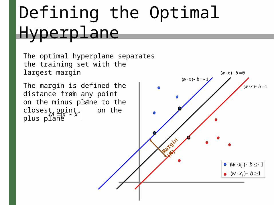
The optimal hyperplane separates the training set with the largest margin
Mar
gin (M
)
Defining the Optimal Hyperplane
(w x) b 0
(w x) b 1
(w x) b 1
(w x i) b 1
(w x i) b 1
The optimal hyperplane separates the training set with the largest margin
Mar
gin (M
)
The margin is defined the distance from any point on the minus plane to the closest point on the plus plane
x
x
M x x

Defining the Optimal Hyperplane
(w x) b 0
(w x) b 1
(w x) b 1
(w x i) b 1
(w x i) b 1
The optimal hyperplane separates the training set with the largest margin
Mar
gin (M
)
The margin is defined the distance from any point on the minus plane to the closest point on the plus plane
x
x
M x x
We need to find M in terms of w

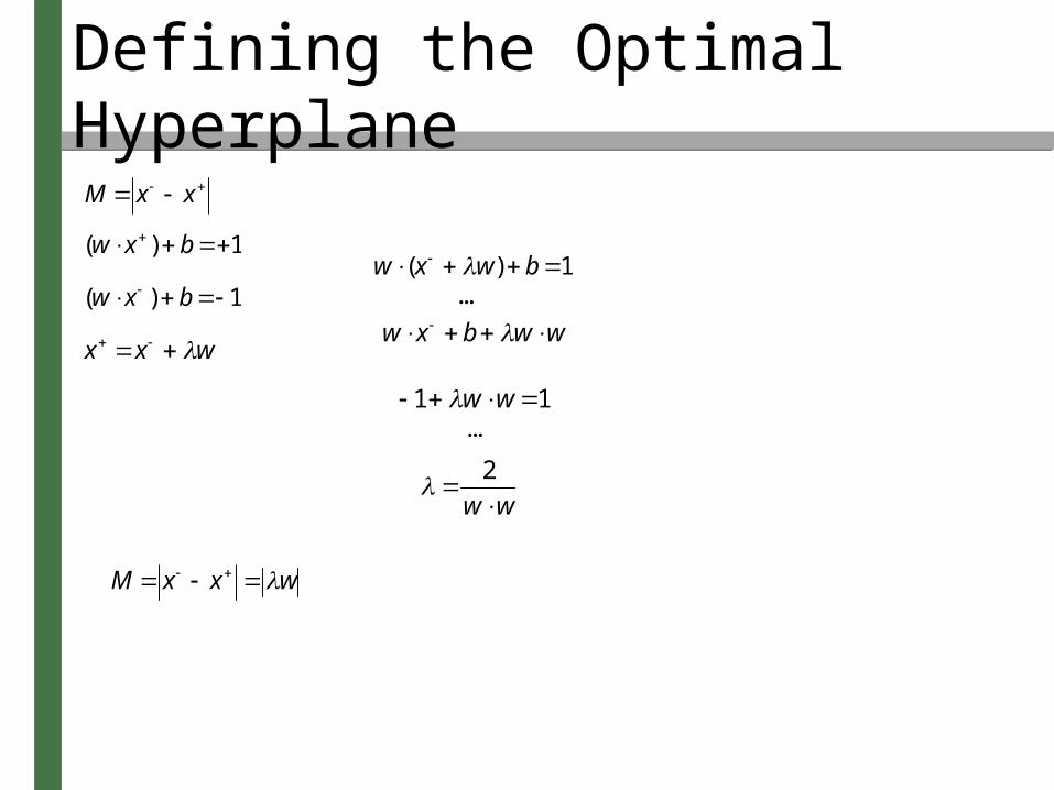
Defining the Optimal Hyperplane
M x x
(w x) b 1
(w x ) b 1
x x wBecause w is perpendicular to the hyperplane

Defining the Optimal Hyperplane
M x x
(w x) b 1
(w x ) b 1
x x w
w (x w) b 1

Defining the Optimal Hyperplane
M x x
(w x) b 1
(w x ) b 1
x x w
w (x w) b 1
w x b w w
…

Defining the Optimal Hyperplane
M x x
(w x) b 1
(w x ) b 1
x x w
w (x w) b 1
w x b w w
…
1 w w 1
2
w w
…
Defining the Optimal Hyperplane
M x x
(w x) b 1
(w x ) b 1
x x w
w (x w) b 1
w x b w w
…
1 w w 1
2
w w
…
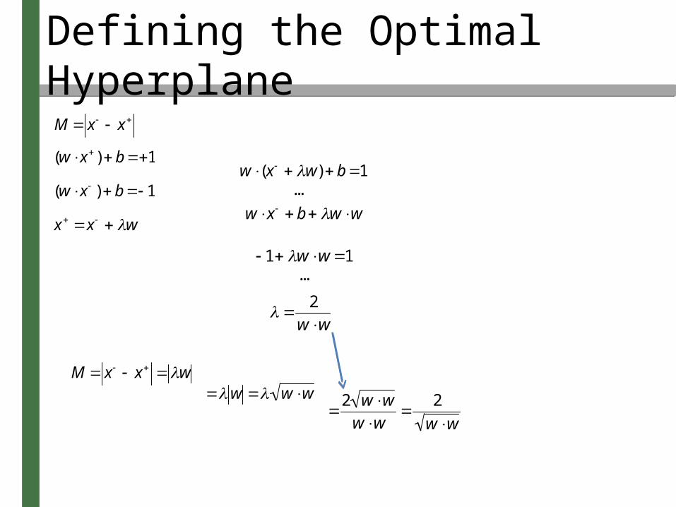
M x x w

Defining the Optimal Hyperplane
M x x
(w x) b 1
(w x ) b 1
x x w
w (x w) b 1
w x b w w
…
1 w w 1
2
w w
…
M x x w
w w w
Defining the Optimal Hyperplane
M x x
(w x) b 1
(w x ) b 1
x x w
w (x w) b 1
w x b w w
…
1 w w 1
2
w w
…
M x x w
w w w
2 w w
w w
2
w w
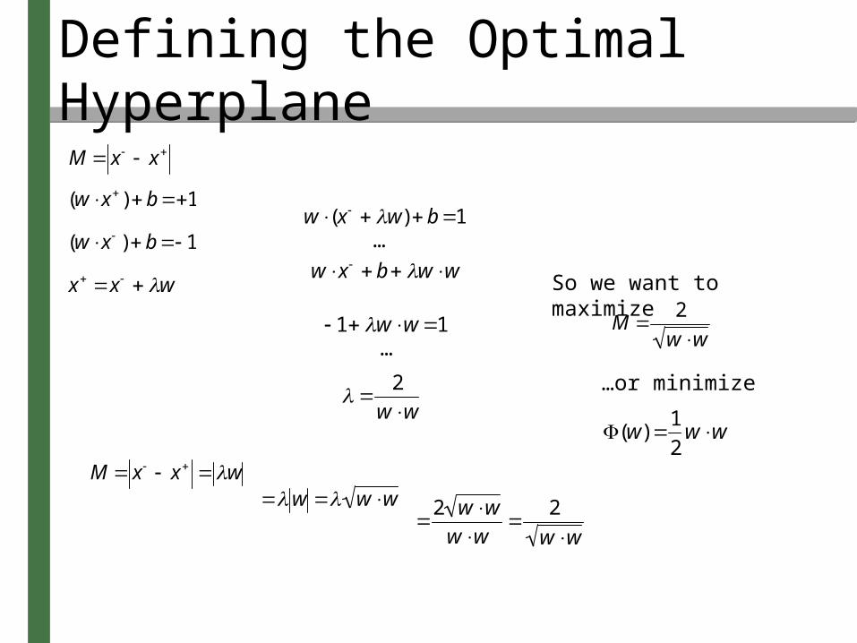
Defining the Optimal Hyperplane
M x x
(w x) b 1
(w x ) b 1
x x w
w (x w) b 1
w x b w w
…
1 w w 1
2
w w
…
M x x w
w w w
2 w w
w w
2
w w
So we want to maximize
M 2
w w
…or minimize
(w) 1
2w w
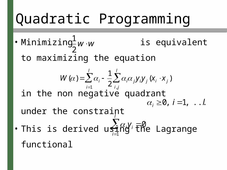
Quadratic Programming
• Minimizing is equivalent to maximizing
the equation
in the non negative quadrant
under the constraint
• This is derived using the Lagrange functional
1
2w w
W () i
i1
l
1
2 i j y iy j (x i x j )
i, j
l
i 0, i 1, ... , l
iy i 0i1
l

• Possible to extend to non-separable training sets by adding a error parameter and minimizing:
• Data can be split into more than two classifications by using successive runs on the resulting classes
Extensions
i
(w,) 1
2(w w) C i
i1
l

• Maps the input vectors into a high-dimensional feature space using a kernel function
• In this feature space the optimal separating hyperplane is constructed
Support Vector (SV) Machines
x
(zi,z) K(x,x i)
Optimal Hyperplane in Feature Space
Feature Space
Input Space

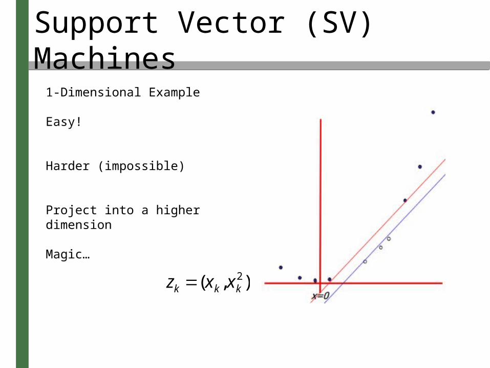
Support Vector (SV) Machines
1-Dimensional Example

Support Vector (SV) Machines
1-Dimensional Example
Easy!

Support Vector (SV) Machines
1-Dimensional Example
Easy!
Harder (impossible)

Support Vector (SV) Machines
1-Dimensional Example
Easy!
Harder (impossible)
Project into a higher dimension
zk (xk, xk2)
Support Vector (SV) Machines
1-Dimensional Example
Easy!
Harder (impossible)
Project into a higher dimension
Magic…
zk (xk, xk2)

• Some possible ways to implement SV machines:i. Polynomial Learning Machinesii. Radial Basis Function Machinesiii. Multi-Layer Neural Networks
• These methods all implement different kernel functions
Support Vector (SV) Machines

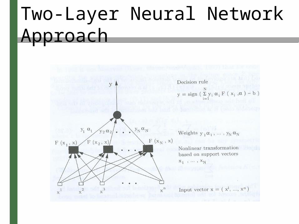
• Kernel is a sigmoid function:• Implements the rules:
• Using this technique the following are found automatically:– Architecture of the two layer machine, determining
the number N of units in the first layer (the number of support vectors)
– The vectors of the weights in the first layer– The vector of weights for the second layer (values of
)
Two-Layer Neural Network Approach
K(x,x i) S v(x x i) c
f (x,) sign iS(v(x x i) c) bi1
N
wi x i
Two-Layer Neural Network Approach
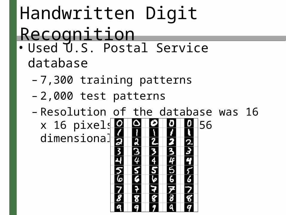
Handwritten Digit Recognition • Used U.S. Postal Service database
– 7,300 training patterns– 2,000 test patterns– Resolution of the database was 16 x 16 pixels
yielding a 256 dimensional input space

Handwritten Digit Recognition
Classifier Raw error%
Human performance 2.5
Decision tree, C4.5 16.2
Polynomial SVM 4.0
RBF SVM 4.1
Neural SVM 4.2

• What are the two components of Generalization Error?
Exam Question 1

• What are the two components of Generalization Error?
Exam Question 1
Approximation Error and Estimation Error

• What is the main difference between Empirical Risk Minimization and Structural Risk Minimization?
Exam Question 2
• What is the main difference between Empirical Risk Minimization and Structural Risk Minimization?
• ERM: Keep the confidence interval fixed (chosen a priori) while minimizing empirical risk
• SRM: Minimize both the confidence interval and the empirical risk simultaneously
Exam Question 2

• What differs between SVM implementations (polynomial, radial, NN, etc.)?
Exam Question 3

• What differs between SVM implementations (polynomial, radial, NN, etc.)?
• The Kernel function.
Exam Question 3

• Vapnik: The Nature of Statistical Learning Theory• Gunn: Support Vector Machines for Classification
and Regression (http://www.dec.usc.es/persoal/cernadas/tc03/mc/SVM.pdf)
• Andrew Moore’s SVM Tutorial: http://www.cs.cmu.edu/~awm/tutorials
References

Any Questions?


