Speech Synthesis byArticulatory Models
Advanced Signal Processing Seminar
Helmuth Ploner-Bernard
Speech Communication and Signal Processing Laboratory
Graz University of Technology
November 12, 2003 – p.1/39
Overview
Introduction
Articulators and (Co-)Articulation
Sound Wave Propagation in the Vocal Tract
The Acoustic Tube Model
Articulatory Models
The “Inverse” Problem of ParameterEstimation
November 12, 2003 – p.2/39
We are . . . here!
Introduction
Articulators and (Co-)Articulation
Sound Wave Propagation in the Vocal Tract
The Acoustic Tube Model
Articulatory Models
The “Inverse” Problem of ParameterEstimation
November 12, 2003 – p.3/39
Introduction – Articulatory Models
Fields of application(Most natural sounding) Speech synthesisLow bit-rate codingSpeech recognitionUnderstanding of human speechproduction
Attempt to describe the actual speechproduction mechanisms
Set of slowly time-varying physiologicalparameters
November 12, 2003 – p.4/39
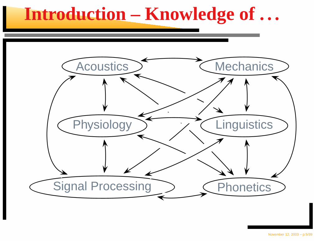
Introduction – Knowledge of . . .
Acoustics Mechanics
Physiology Linguistics
Signal Processing Phonetics
November 12, 2003 – p.5/39
Introduction
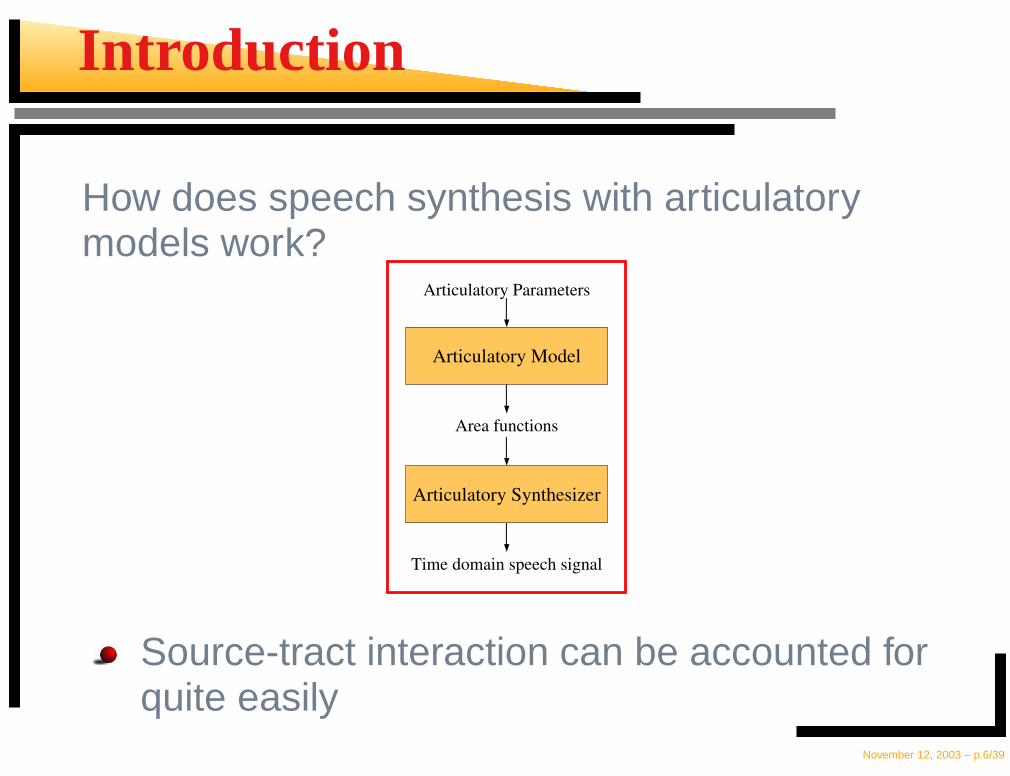
How does speech synthesis with articulatorymodels work?
Articulatory Model
Articulatory Synthesizer
Articulatory Parameters
Area functions
Time domain speech signal
Source-tract interaction can be accounted forquite easily
November 12, 2003 – p.6/39
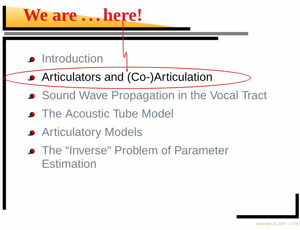
We are . . . here!
Introduction
Articulators and (Co-)Articulation
Sound Wave Propagation in the Vocal Tract
The Acoustic Tube Model
Articulatory Models
The “Inverse” Problem of ParameterEstimation
November 12, 2003 – p.7/39
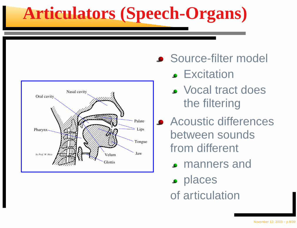
Articulators (Speech-Organs)
Lips
Tongue
JawVelum
Glottis
Pharynx
Oral cavity
Nasal cavity
by Prof. W. Hess
Palate
Source-filter modelExcitationVocal tract doesthe filtering
Acoustic differencesbetween soundsfrom different
manners andplaces
of articulation
November 12, 2003 – p.8/39
(Co-)Articulation
Articulation of an (isolated) phoneme involves“Critical” articulators, essential for correctproduction“Non-critical” articulators, place andmanner unspecified
Co-articulation in fluent speechTarget positions of articulators stronglyaffected by each otherDependent on phonetic context
November 12, 2003 – p.9/39
(Co-)Articulation
Associate priorities with parameters ofarticulatory model and let your controllerexploit them
Incorporate realistic physiological anddynamic constraints (cf. functional models)
→ more natural sounding speech
November 12, 2003 – p.10/39
We are . . . here!
Introduction
Articulators and (Co-)Articulation
Sound Wave Propagation in the Vocal Tract
The Acoustic Tube Model
Articulatory Models
The “Inverse” Problem of ParameterEstimation
November 12, 2003 – p.11/39
Wave Propagation
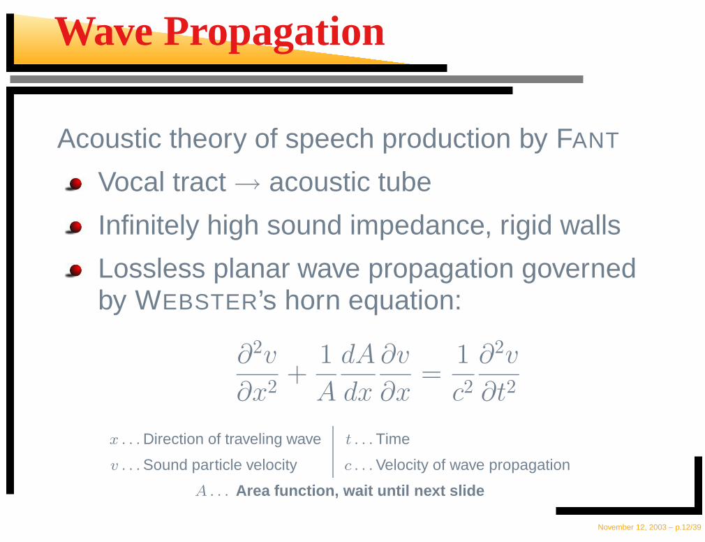
Acoustic theory of speech production by FANT
Vocal tract → acoustic tube
Infinitely high sound impedance, rigid walls
Lossless planar wave propagation governedby WEBSTER’s horn equation:
∂2v
∂x2+
1
A
dA
dx
∂v
∂x=
1
c2
∂2v
∂t2
x . . . Direction of traveling wave t . . . Time
v . . . Sound particle velocity c . . . Velocity of wave propagation
A . . . Area function, wait until next slide
November 12, 2003 – p.12/39
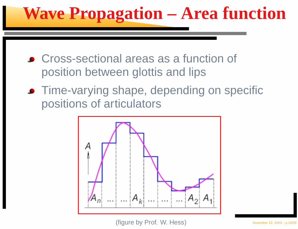
Wave Propagation – Area function
Cross-sectional areas as a function ofposition between glottis and lips
Time-varying shape, depending on specificpositions of articulators
(figure by Prof. W. Hess) November 12, 2003 – p.13/39
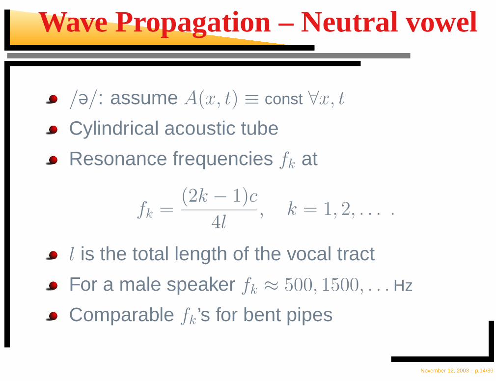
Wave Propagation – Neutral vowel
/@/: assume A(x, t) ≡ const ∀x, t
Cylindrical acoustic tube
Resonance frequencies fk at
fk =(2k − 1)c
4l, k = 1, 2, . . . .
l is the total length of the vocal tract
For a male speaker fk ≈ 500, 1500, . . . Hz
Comparable fk’s for bent pipes
November 12, 2003 – p.14/39
Wave Propagation
Horn equation cannot be solved for arbitrary areafunction
Changes in vocal tract shape lead to changes inEigenfrequencies
November 12, 2003 – p.15/39
Wave Propagation
Horn equation cannot be solved for arbitrary areafunction
Changes in vocal tract shape lead to changes inEigenfrequencies
At f = 3.5 kHz first cross-modes in vocal tract
, most of the energy in speech signals concentratedin region below this frequency
November 12, 2003 – p.15/39
Wave Propagation
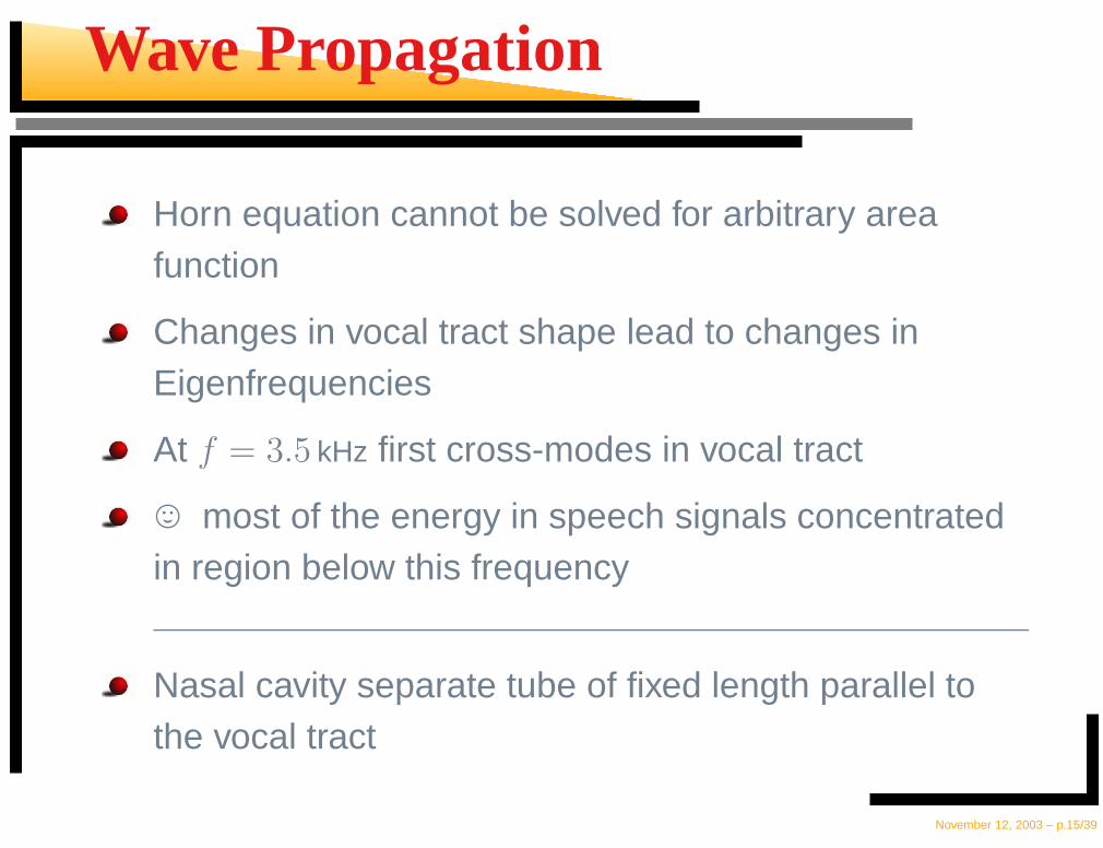
Horn equation cannot be solved for arbitrary areafunction
Changes in vocal tract shape lead to changes inEigenfrequencies
At f = 3.5 kHz first cross-modes in vocal tract
, most of the energy in speech signals concentratedin region below this frequency
Nasal cavity separate tube of fixed length parallel tothe vocal tract
November 12, 2003 – p.15/39
We are . . . here!
Introduction
Articulators and (Co-)Articulation
Sound Wave Propagation in the Vocal Tract
The Acoustic Tube Model
Articulatory Models
The “Inverse” Problem of ParameterEstimation
November 12, 2003 – p.16/39
The Acoustic Tube Model
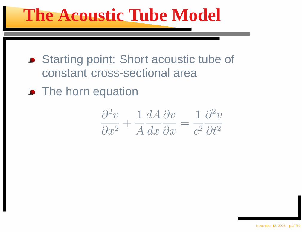
Starting point: Short acoustic tube ofconstant cross-sectional area
The horn equation
∂2v
∂x2+
1
A
dA
dx
∂v
∂x=
1
c2
∂2v
∂t2
November 12, 2003 – p.17/39
The Acoustic Tube Model
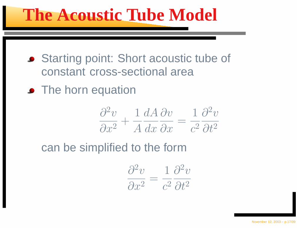
Starting point: Short acoustic tube ofconstant cross-sectional area
The horn equation
∂2v
∂x2+
1
A
dA
dx
∂v
∂x=
1
c2
∂2v
∂t2
can be simplified to the form
∂2v
∂x2=
1
c2
∂2v
∂t2
November 12, 2003 – p.17/39
The Acoustic Tube Model
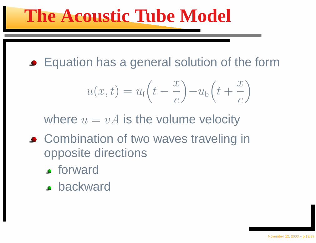
Equation has a general solution of the form
u(x, t) = uf
(
t −x
c
)
−ub
(
t +x
c
)
where u = vA is the volume velocity
Combination of two waves traveling inopposite directions
forwardbackward
November 12, 2003 – p.18/39
The Acoustic Tube Model
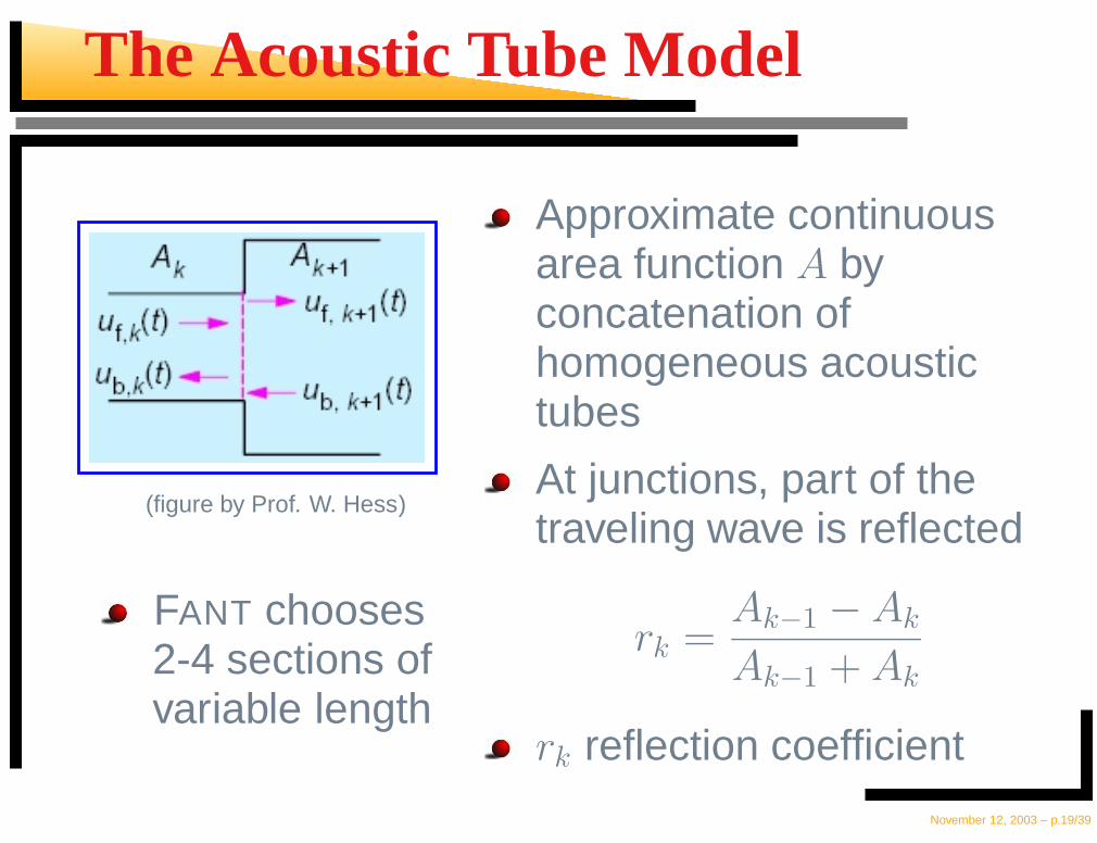
(figure by Prof. W. Hess)
FANT chooses2-4 sections ofvariable length
Approximate continuousarea function A byconcatenation ofhomogeneous acoustictubes
At junctions, part of thetraveling wave is reflected
rk =Ak−1 − Ak
Ak−1 + Ak
rk reflection coefficient
November 12, 2003 – p.19/39
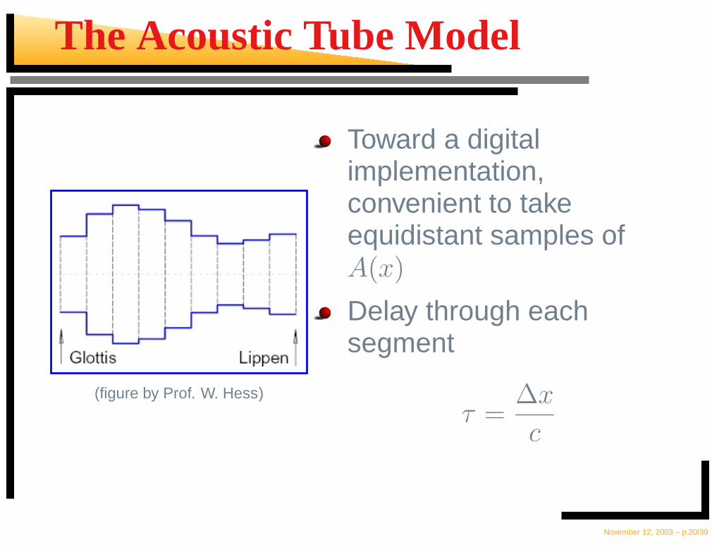
The Acoustic Tube Model
(figure by Prof. W. Hess)
Toward a digitalimplementation,convenient to takeequidistant samples ofA(x)
Delay through eachsegment
τ =∆x
c
November 12, 2003 – p.20/39
The Acoustic Tube Model
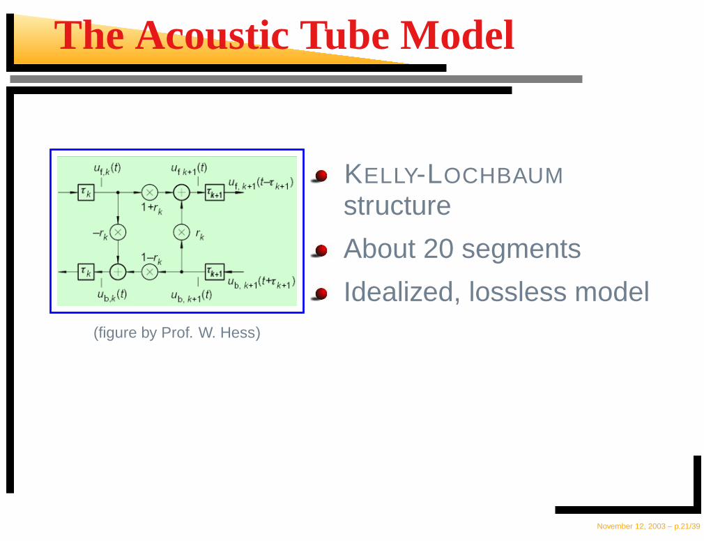
(figure by Prof. W. Hess)
KELLY-LOCHBAUMstructure
About 20 segments
Idealized, lossless model
November 12, 2003 – p.21/39
The Acoustic Tube Model – Losses
In reality, losses occur due toResonances of yielding wallsViscous and thermal losses along the pathof propagation → add multipliersRadiation at the lips → insert additionalsegment in front of the lips
Freeze delay τ to any given sampling intervalWave digital filters
November 12, 2003 – p.22/39
We are . . . here!
Introduction
Articulators and (Co-)Articulation
Sound Wave Propagation in the Vocal Tract
The Acoustic Tube Model
Articulatory Models
The “Inverse” Problem of ParameterEstimation
November 12, 2003 – p.23/39
Articulatory Models – Static
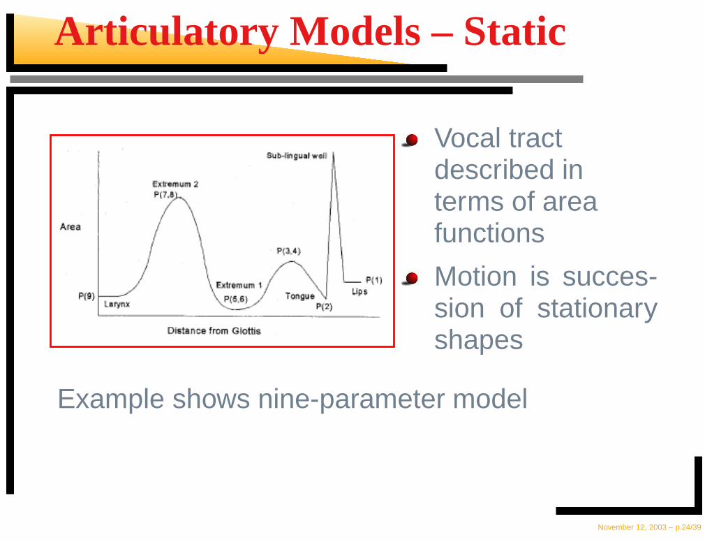
Vocal tractdescribed interms of areafunctions
Motion is succes-sion of stationaryshapes
Example shows nine-parameter model
November 12, 2003 – p.24/39
Articulatory Models – Dynamic
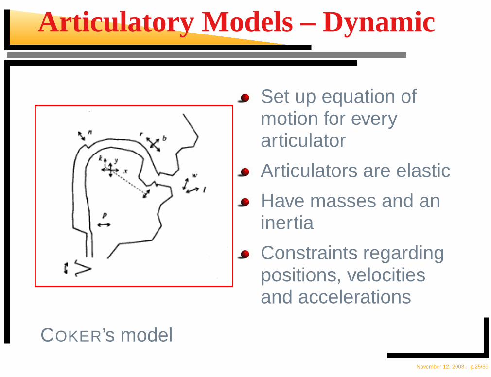
Set up equation ofmotion for everyarticulator
Articulators are elastic
Have masses and aninertia
Constraints regardingpositions, velocitiesand accelerations
COKER’s modelNovember 12, 2003 – p.25/39
We are . . . here!
Introduction
Articulators and (Co-)Articulation
Sound Wave Propagation in the Vocal Tract
The Acoustic Tube Model
Articulatory Models
The “Inverse” Problem of ParameterEstimation
November 12, 2003 – p.26/39
Parameter Estimation (1)
“Inverse” problem
Acquire model parameters directly orindirectly from speech signal
Most difficult
Non-unique, i. e. more than one vocal tractshape can produce signal with identicalspectrum
November 12, 2003 – p.27/39
Parameter Estimation (2)
Required:Good acoustic matchingSmooth evolution of area functions orarticulatory parametersAnatomical feasibility
Most methods are unable to determine vocaltract length
November 12, 2003 – p.28/39
Parameter Estimation – MRI (1)
Most intuitive way
“Measure” vocal tract shape directly
Several scans necessary for 3D-model (howcan we represent /l/ with mid-sagittal areafunctions?)
Much signal processing to be done here
Costly, time consuming and noisy
November 12, 2003 – p.29/39
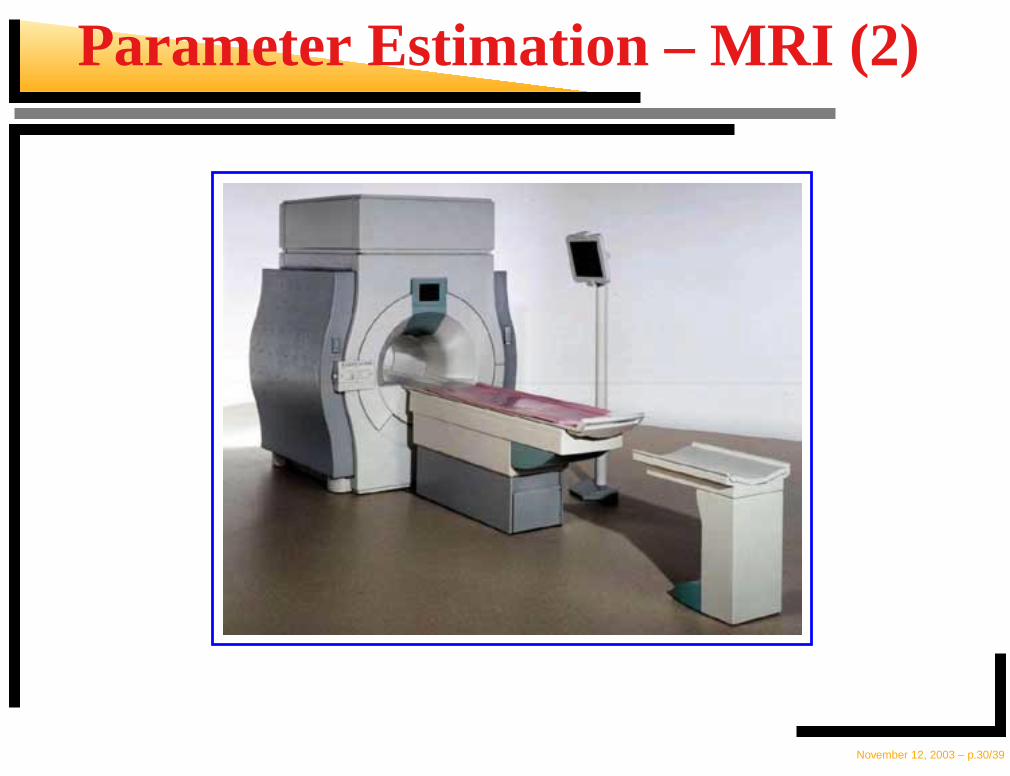
Parameter Estimation – MRI (2)
November 12, 2003 – p.30/39
Parameter Estimation – LPC
Simple, cheap method
Evaluate reflection coefficients fromLEVINSON-DURBIN algorithm for LinearPredictive Coding
Characterize an idealized acoustic tubemodel
Obtained from real world lossy signals
� Inaccurate results
November 12, 2003 – p.31/39
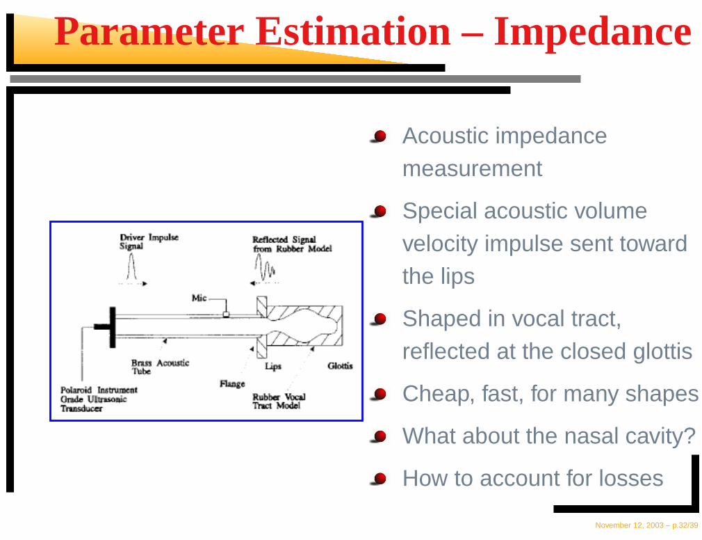
Parameter Estimation – Impedance
Acoustic impedancemeasurement
Special acoustic volumevelocity impulse sent towardthe lips
Shaped in vocal tract,reflected at the closed glottis
Cheap, fast, for many shapes
What about the nasal cavity?
How to account for losses
November 12, 2003 – p.32/39
Parameter Estimation – ABS
ABS: Analysis by Synthesis
Method for automated parameter identification from natural
utterances
Algorithm:
Extract descriptive parameters from signal
Look up “best matching” articulatory parameters in
codebook
Re-synthesize with articulatory parameter set
Compare re-synthesized signal to target speech signal
(original)
Iteratively optimize parameters
November 12, 2003 – p.33/39
Parameter Estimation – ABS
SegmentationPhoneme basis, variable lengthFixed frame lengths
Time alignment, pitch synchronous analysesto avoid influence of glottal excitation
Descriptive parametersLPC-coefficientsMel frequency cepstral coefficientsCoefficients of any spectral transformation
November 12, 2003 – p.34/39
Parameter Estimation – ABS
Remember: Mapping is non-unique
Find other shapes of vocal tract according toa cost function
Components of cost functionDistance between spectraSmoothness of area functionSmooth evolution of parameters betweenadjacent framesSignal energy
Improvement: multi-frame optimizationNovember 12, 2003 – p.35/39
Optional: Generation of the codebook
Random sampling
Iterate through various configurations of articulatory
parameters
Store along with their corresponding descriptive
parameters
Huge amount of items
Unnecessary data not used in language or by a speaker
“Inching” approach
Start out at extreme articulatory parameters
Interpolations on trajectories in articulatory space
Attention to sparsely populated areas
November 12, 2003 – p.36/39
Summary
Wave propagation in the vocal tract
Area function responsible for different sounds
Co-articulation with priority parameters
Non-unique acoustic-to-articulatory mapping
Tube model, KELLY-LOCHBAUM structure,WDF
Static models, dynamic models
Parameter estimation: MRI, LPC, Impedancemeasurement, ABS
November 12, 2003 – p.37/39
References
http://www.ikp.uni-bonn.de/dt/lehre/materialien/aap/aap_1f.pdf
http://www.radiologyinfo.org/
J.W. Devaney and C. C. Goodyear. A comparison of acoustic and magneticresonance imaging techniques in the estimation of vocal tract area functions.International Symposium on Speech, Image Processing and Neural Networks,pages 575–578, April 1994.
A. R. Greenwood and C. C. Goodyear. Articulatory speech synthesis using aparametric model and a polynomial mapping technique. International symposiumon speech, image processing and neural networks, pages 595–598, April 1994
S. Parthasarathy and C.H. Coker. Phoneme-level parametrization of speech usingan articulatory model. International Conference on Acoustics, Speech and SignalProcessing, pages 337–340, April 1990
Peter Vary, Ulrich Heute, and Wolfgang Hess. Digitale Sprachsignalverarbeitung.B.G. Teubner Stuttgart, 1998
November 12, 2003 – p.38/39

Thank you for your attention!
Have a look at the accompanyingpaper on the web!
November 12, 2003 – p.39/39


