
enginf
SPARE PARTS MANAGEMENT FOR NUCLEAR POWER GENERATION FACILITIES
by
Natalie Michele Scala
B.S. Mathematics, John Carroll University, 2005
M.S. Industrial Engineering, University of Pittsburgh, 2007
Submitted to the Graduate Faculty of
Swanson School of Engineering in partial fulfillment
of the requirements for the degree of
Doctor of Philosophy
University of Pittsburgh
2011

ii
UNIVERSITY OF PITTSBURGH
SWANSON SCHOOL OF ENGINEERING
This dissertation was presented
by
Natalie Michele Scala
It was defended on
June 21, 2011
and approved by
Mary Besterfield-Sacre, Associate Professor, Department of Industrial Engineering
Bryan Norman, Associate Professor, Department of Industrial Engineering
Luis Vargas, Professor, Joseph M. Katz Graduate School of Business
Dissertation Co-Director: Jayant Rajgopal, Associate Professor, Department of Industrial
Engineering
Dissertation Co-Director: Kim Needy, Professor and Department Head, Department of
Industrial Engineering, University of Arkansas

iii
Copyright © by Natalie Michele Scala
2011

iv
With deregulation, utilities in the power sector face a much more urgent imperative to
emphasize cost efficiencies as compared to the days of regulation. One major opportunity for
cost savings is through reductions in spare parts inventories. Most utilities are accustomed to
carrying large volumes of expensive, relatively slow-moving parts because of a high degree of
risk-averseness. This attitude towards risk is rooted in the days of regulation. Under regulation,
companies recovered capital inventory costs by incorporating them into the base rate charged to
their customers. In a deregulated environment, cost recovery is no longer guaranteed.
Companies must therefore reexamine their risk profile and develop policies for spare parts
inventory that are appropriate for a competitive business environment.
This research studies the spare parts inventory management problem in the context of
electric utilities, with a focus on nuclear power. It addresses three issues related to this problem:
criticality, risk, and policy. With respect to criticality and risk, a methodology is presented that
incorporates the use of influence diagrams and the Analytic Hierarchy Process (AHP). A new
method is developed for group aggregation in the AHP when Saaty and Vargas’ (2007)
dispersion test fails and decision makers are unwilling or unable to revise their judgments. With
respect to policy, a quantitative model that ranks the importance of keeping a part in inventory
and recommends a corresponding stocking policy through the use of numerical simulation is
developed.
SPARE PARTS MANAGEMENT FOR NUCLEAR POWER GENERATION
FACILITIES
Natalie Michele Scala, PhD
University of Pittsburgh, 2011

v
This methodology and its corresponding models will enable utilities that have
transitioned from a regulated to a deregulated environment become more competitive in their
operations while maintaining safety and reliability standards. Furthermore, the methodology
developed is general enough so that other utility plants, especially those in the nuclear sector,
will be able to use this approach. In addition to regulated utilities, other industries, such as
aerospace, and the military can also benefit from extensions to these models, as risk profiles and
subsequent policies can be adjusted to align with the business environment in which each
industry or company operates.

vi
TABLE OF CONTENTS
ACKNOWLEDGMENTS .................................................................................................... XVIII 1.0 PROBLEM STATEMENT ......................................................................................... 1
1.1 RESEARCH STATEMENT ............................................................................... 1
1.2 BACKGROUND ON ELECTRIC UTILITIES ................................................ 2
1.3 DEREGULATION AND SPARE PARTS......................................................... 4
1.4 CURRENT PARTS PROCESS .......................................................................... 7
1.5 RESEARCH FOCUS........................................................................................... 9
2.0 APPROACH AND METHODOLOGY ................................................................... 13 2.1 FORECASTING METHODS ........................................................................... 13
2.2 PART DEMANDS AT NUCLEAR PLANTS ................................................. 15
2.3 DATA COLLECTION ...................................................................................... 16
2.4 FORECASTING DEMAND ............................................................................. 20
2.5 FAILURE RATES AND PREVENTATIVE MAINTENANCE ................... 25
2.6 COST TRADEOFFS ......................................................................................... 26
2.7 SUBJECTIVE RISK AND NUCLEAR POWER ........................................... 29
2.7.1 Risk ................................................................................................................. 29
2.7.2 Employee Level of Risk ................................................................................. 30
2.7.3 Public Perceptions of Risk ............................................................................ 34
vii
2.8 RISK OF REVENUE LOSS ............................................................................. 37
2.9 FOUR STEP METHODOLOGY ..................................................................... 39
3.0 INFLUENCE DIAGRAM ......................................................................................... 43
3.1 BACKGROUND ................................................................................................ 43
3.1.1 Examples of Use of Influence Diagrams ...................................................... 44
3.2 MODELING THE SPARE PARTS PROCESS IN NUCLEAR PLANTS .. 44
3.3 INFLUENCE DIAGRAM MODEL ................................................................. 45
3.3.1 Influence Set Descriptions............................................................................. 50
3.4 JUDGEMENT OF INFLUENCES .................................................................. 53
3.5 VALIDATION ................................................................................................... 54
3.6 SUMMARY ........................................................................................................ 55
4.0 INTERVIEW PROTOCOL AND USE OF THE ANALYTIC HIERARCHY PROCESS (AHP) ................................................................................................................ 56
4.1 BACKGROUND ON THE AHP ...................................................................... 56
4.2 EXAMPLES OF USE OF THE AHP .............................................................. 57
4.3 GROUP JUDGEMENTS IN THE AHP .......................................................... 58
4.4 INTERVIEW PROTOCOL .............................................................................. 59
4.5 AN EXAMPLE OF EMPLOYEE RESPONSES ............................................ 65
4.6 GROUP AGGREGATION ............................................................................... 69
4.7 SUMMARY ........................................................................................................ 72
5.0 PRINCIPAL COMPONENTS ANALYSIS (PCA) BASED METHOD FOR GROUP AGGREGATION IN THE ANALYTIC HIERARCHY PROCESS (AHP) ................. 74
5.1 MOTIVATION FOR PCA BASED METHOD .............................................. 74
5.2 OVERVIEW OF PCA ....................................................................................... 78
viii
5.3 PRINCIPAL COMPONENTS AND THE AHP ............................................. 79
5.4 ILLUSTRATIVE EXAMPLE .......................................................................... 81
5.5 CONVERGENCE OF VP TO VG...................................................................... 83
5.6 SUMMARY ........................................................................................................ 90
6.0 PART CRITICALITY SCORES AND CLASSIFICATION ................................. 92
6.1 LITERATURE REVIEW ................................................................................. 92
6.2 SELECTION OF SAMPLE DATA ................................................................. 97
6.3 ORDINAL PART DATA .................................................................................. 98
6.3.1 Influence 2.1: Failure of Part Leads to LCO or SPV ............................... 101
6.3.2 Influence 1.3: Immediacy of Schedule—When to Complete the Work Order ............................................................................................................ 102
6.4 SCALE ASSIGNMENTS ................................................................................ 103
6.5 CRITICALITY SCORING MODEL ............................................................ 109
6.6 SCORING EQUATIONS EXAMPLE ........................................................... 110
6.7 GROUPING OF PARTS ................................................................................. 112
6.8 VALIDATION ................................................................................................. 116
6.9 SUMMARY ...................................................................................................... 116
7.0 INVENTORY MANAGEMENT POLICY............................................................ 118
7.1 COMMON INVENTORY SYSTEMS ........................................................... 118
7.2 LEAD TIME ANALYSIS ............................................................................... 121
7.3 HISTORICAL SIMULATION....................................................................... 125
7.4 CALCULATING AVERAGE EFFECTIVE DEMAND PER PLANT REQUEST ........................................................................................................ 127
7.4.1 Calculating the Lower Bound of zk ............................................................ 129

ix
7.4.2 Calculating the Upper Bound of zk ............................................................. 130
7.4.3 Calculating an Intermediate Value of zk .................................................... 130
7.5 RESULTS AND DISCUSSION ...................................................................... 131
7.5.1 Special Attention Parts ................................................................................ 135
7.5.2 Refined Base Stock Policy ........................................................................... 136
7.5.3 Other Groups and Versions of Code.......................................................... 140
7.6 SUMMARY ...................................................................................................... 141
8.0 SUMMARY AND CONCLUSIONS ...................................................................... 143
8.1 SUMMARY AND CONTRIBUTIONS OF METHODOLOGY ................. 144
8.2 EXTENDED CONTRIBUTIONS .................................................................. 148
8.3 FUTURE WORK ............................................................................................. 150
APPENDIX A ............................................................................................................................ 152
APPENDIX B ............................................................................................................................ 159
APPENDIX C ............................................................................................................................ 171
BIBLIOGRAPHY ..................................................................................................................... 223
x
LIST OF TABLES
Table 1. Day-ahead LMP summary statistics ............................................................................... 28
Table 2. Influences in the spare parts ordering process along with node connections ................. 49
Table 3. Summary of influence sets .............................................................................................. 51
Table 4. Employees, work locations, job functions and influence sets for pairwise comparison interviews ....................................................................................................................... 60
Table 5. Ratio scale values and corresponding values (Saaty, 1980; 1990) ................................. 62
Table 6. Revised judgments for all respondents in the “Timeliness of Work Order” set ............. 69
Table 7. Aggregated group judgments for the “Timeliness of Work Order” set .......................... 71
Table 8. Synthesized priorities from aggregated AHP judgments for all influence sets .............. 72
Table 9. Illustrative example judgments ....................................................................................... 81
Table 10. Symmetric matrix SP for computing the AHP priorities ............................................... 82
Table 11. Symmetric matrix SG for computing the AHP priorities .............................................. 83
Table 12. Saaty’s Fundamental Scale values assigned to units .................................................... 84
Table 13. Probability (𝒂𝒎𝜹)/100 that the dispersion test fails under a scale spread of δ ............ 87
Table 14. Part characteristic data for all influences .................................................................... 104
Table 15. Centroids tested in k-means algorithm ........................................................................ 115
Table 16. Descriptive statistics for final k-means analysis ......................................................... 115
Table 17. Hypothetical movement data for part F ...................................................................... 128

xi
Table 18. Simulation results for all parts in group I and intermediate demand estimate ........... 133
Table 19. Parts that contribute to delayed work days at LCO locations ..................................... 136
Table 20. Simulation results for LCO parts in group I and intermediate demand estimate ....... 137
Table 21. Simulation results for non-LCO parts in group I and intermediate demand estimate 139
Table 22. Description of influences in the “Timeliness of Work Order” set .............................. 156
Table 23. Description of influences in the “Part Failure” set ..................................................... 156
Table 24. Description of influences in the “Vendor Availability” set ........................................ 157
Table 25. Description of influences in the “Part Usage in Plant” set ......................................... 157
Table 26. Description of influences in the “Preventative Maintenance Schedule” set ............... 158
Table 27. Description of influences in the “Outage Usage” set ................................................. 158
Table 28. Description of influences in the “Cost Consequences” set ......................................... 158
Table 29. Pairwise comparisons for the “Timeliness of Work Order” set .................................. 160
Table 30. Pairwise comparisons for the “Part Failure” set ......................................................... 161
Table 31. Pairwise comparisons for the “Vendor Availability” set ............................................ 162
Table 32. Pairwise comparisons for the “Part Usage in Plant” set ............................................. 163
Table 33. Pairwise comparisons for the “Preventative Maintenance Schedule” set ................... 164
Table 34. Pairwise comparisons for the “Outage Usage” set ..................................................... 165
Table 35. Pairwise comparisons for the “Cost Consequences” set ............................................. 165
Table 36. Pairwise comparisons for the set of overall influences ............................................... 165
Table 37. Revised judgments for all respondents in the “Part Failure” set ................................ 166
Table 38. Revised judgments for all respondents in the “Vendor Availability” set ................... 166
Table 39. Revised judgments for all respondents in the “Part Usage” set .................................. 167
Table 40. Revised judgments for all respondents in the “Preventative Maintenance Schedule” set .................................................................................................................................... 167

xii
Table 41. Revised judgments for all respondents in the “Outage Usage” set ............................ 167
Table 42. Revised judgments for all respondents in the “Cost Consequences” set .................... 168
Table 43. Revised judgments for all respondents in the set of overall influences ...................... 168
Table 44. Aggregated group judgments for the “Part Failure” set ............................................. 168
Table 45. Aggregated group judgments for the “Vendor Availability” set ................................ 169
Table 46. Aggregated group judgments for the “Part Usage in Plant” set ................................. 169
Table 47. Aggregated judgments for the “Preventative Maintenance Schedule” set ................. 169
Table 48. Aggregated judgments for the “Outage Usage” set .................................................... 170
Table 49. Aggregated judgments for the “Cost Consequences” set ........................................... 170
Table 50. Aggregated judgments for the set of overall influences ............................................. 170
Table 51. Simulation results for all parts in group I and demand underestimated ..................... 180
Table 52. Simulation results for non-LCO parts in group 1 and demand underestimated ......... 182
Table 53. Simulation results for LCO parts in group I and demand underestimated ................. 184
Table 54. Simulation results for all parts in group I and demand overestimated ....................... 185
Table 55. Simulation results for non-LCO parts in group I and demand overestimated ............ 187
Table 56. Simulation results for LCO parts in group I and demand overestimated ................... 189
Table 57. Simulation results for all parts in group II and demand underestimated .................... 189
Table 58. Simulation results for non-LCO parts in group II and demand underestimated ......... 194
Table 59. Simulation results for LCO parts in group II and demand underestimated ................ 197
Table 60. Simulation results for all parts in group II and demand overestimated ...................... 198
Table 61. Simulation results for non-LCO parts in group II and demand overestimated ........... 201
Table 62. Simulation results for LCO parts in group II and demand overestimated .................. 202
Table 63. Simulation results for all parts in group II and intermediate demand estimate .......... 203
xiii
Table 64. Simulation results for non-LCO parts in group II and intermediate demand estimate 206
Table 65. Simulation results for LCO parts in group II and intermediate demand estimate ...... 208
Table 66. Simulation results for all parts in group III and demand underestimated ................... 209
Table 67. Simulation results for non-LCO parts in group III and demand underestimated ....... 212
Table 68. Simulation results for LCO parts in group III and demand underestimated ............... 213
Table 69. Simulation results for all parts in group III and demand overestimated ..................... 214
Table 70. Simulation results for non-LCO parts in group III and demand overestimated ......... 216
Table 71. Simulation results for LCO parts in group III and demand overestimated ................. 218
Table 72. Simulation results for all parts in group III and intermediate demand estimate ......... 218
Table 73. Simulation results for non-LCO parts in group III and intermediate demand estimate .................................................................................................................................... 221
Table 74. Simulation results for LCO parts in group III and intermediate demand estimate ..... 221

xiv
LIST OF FIGURES
Figure 1. Cumulative on hand inventory level for part A ............................................................. 18
Figure 2. Raw demand versus actual demand for part A .............................................................. 19
Figure 3. Reasons for demand ...................................................................................................... 19
Figure 4. Exponential smoothing forecast .................................................................................... 21
Figure 5. Intermittent demand forecasts for part B ....................................................................... 23
Figure 6. Intermittent demand forecasts for part C ....................................................................... 23
Figure 7. Adaptation of general job and accident risk graph (Sjöberg & Sjöberg, 1991) ............ 32
Figure 8. Influence diagram node example ................................................................................... 43
Figure 9. High level influence diagram, with sub-level influence diagram for the “Timeliness of Work Order” set ........................................................................................................... 48
Figure 10. Sample hierarchy with 3 attributes and 5 alternatives ................................................. 57 Figure 11. “Timeliness of Work Order” set AHP hierarchy ......................................................... 63
Figure 12. Employee #15 original judgments ............................................................................... 66
Figure 13. Employee #15 original priorities and inconsistency ................................................... 66
Figure 14. Employee #18 original judgments ............................................................................... 66
Figure 15. Employee #18 original priorities and inconsistency ................................................... 66
Figure 16. Employee #15 revised judgments ................................................................................ 68
Figure 17. Employee #15 revised priorities .................................................................................. 68

xv
Figure 18. Employee #18 revised judgments ................................................................................ 68
Figure 19. Employee #18 revised priorities and inconsistency .................................................... 69
Figure 20. Probability (𝒂𝒎𝜹)/100 that the dispersion test fails under a scale spread of δ .......... 87
Figure 21. Distance d as a function of δ for values of f ................................................................ 89
Figure 22. Histogram of part scores ............................................................................................ 113
Figure 23. Histogram of part scores with suggested groups of parts .......................................... 113
Figure 24. Lead time histogram for part a250 ............................................................................ 122
Figure 25. Lead time histogram for part b166 ............................................................................ 123
Figure 26. Lead time histogram for part a65 .............................................................................. 123
Figure 27. All parts vs. all non-LCO missed days for group I and intermediate demand estimate ................................................................................................................................... 134
Figure 28. All parts vs. all LCO missed days for group I and intermediate demand estimate ... 134
Figure 29. LCO parts vs. LCO missed days for group I and intermediate demand estimate ..... 137
Figure 30. Non-LCO parts vs. non-LCO missed days for group I and intermediate demand estimate ..................................................................................................................... 138
Figure 31. Influence sub-diagram for the “Timeliness of Work Order” set ............................... 152
Figure 32. Influence sub-diagram for the “Part Failure” set ....................................................... 153
Figure 33. Influence sub-diagram for the “Vendor Availability” set ......................................... 153
Figure 34. Influence sub-diagram for the “Part Usage in Plant” set ........................................... 154
Figure 35. Influence sub-diagram for the “Preventative Maintenance Schedule” set ................ 154
Figure 36. Influence sub-diagram for the “Outage Usage” set ................................................... 155
Figure 37. Influence sub-diagram for the “Cost Consequences” set .......................................... 155
Figure 38. All parts vs. all non-LCO missed days for group I and demand underestimated ...... 181
Figure 39. All parts vs. all LCO missed days for group I and demand underestimated ............. 181

xvi
Figure 40. Non-LCO parts vs. non-LCO missed days for group I and demand underestimated 183
Figure 41. LCO parts vs. LCO missed days for group I and demand underestimated ............... 183
Figure 42. All parts vs. all non-LCO missed days for group I and demand overestimated ........ 186
Figure 43. All parts vs. all LCO missed days for group I and demand overestimated ............... 186
Figure 44. Non-LCO parts vs. non-LCO missed days for group I and demand overestimated .. 188
Figure 45. LCO parts vs. LCO missed days for group I and demand overestimated ................. 188
Figure 46. All parts vs. all non-LCO missed days for group II and demand underestimated .... 192
Figure 47. All parts vs. all LCO missed days for group II and demand underestimated ............ 193
Figure 48. Non-LCO parts vs. non-LCO missed days for group II and demand underestimated ................................................................................................................................... 193
Figure 49. LCO parts vs. LCO missed days for group II and demand underestimated .............. 196 Figure 50. All parts vs. all non-LCO missed days for group II and demand overestimated ...... 199 Figure 51. All parts vs. all LCO missed days for group II and demand overestimated .............. 200
Figure 52. Non-LCO parts vs. non-LCO missed days for group II and demand overestimated 200
Figure 53. LCO parts vs. LCO missed days for group II and demand overestimated ................ 203
Figure 54. All parts vs. all non-LCO missed days for group II and intermediate demand estimate ................................................................................................................................... 205
Figure 55. All parts vs. all LCO missed days for group II and intermediate demand estimate .. 205
Figure 56. Non-LCO parts vs. non-LCO missed days for group II and intermediate demand estimate ..................................................................................................................... 207
Figure 57. LCO parts vs. LCO missed days for group II and intermediate demand estimate .... 209
Figure 58. All parts vs. all non-LCO missed days for group III and demand underestimated ... 210
Figure 59. All parts vs. all LCO missed days for group III and demand underestimated .......... 211
Figure 60. Non-LCO parts vs. non-LCO missed days for group III and demand underestimated ................................................................................................................................... 211

xvii
Figure 61. LCO parts vs. LCO missed days for group III and demand underestimated ............ 213
Figure 62. All parts vs. all non-LCO missed days for group III and demand overestimated ..... 215
Figure 63. All parts vs. all LCO missed days for group III and demand overestimated ............ 215
Figure 64. Non-LCO parts vs. non-LCO missed days for group III and demand overestimated 217
Figure 65. LCO parts vs. LCO missed days for group III and demand overestimated .............. 217
Figure 66. All parts vs. all non-LCO missed days for group III and intermediate demand estimate ................................................................................................................................... 219
Figure 67. All parts vs. all LCO missed days for group III and intermediate demand estimate 220 Figure 68. Non-LCO parts vs. non-LCO missed days for group III and intermediate demand
estimate ..................................................................................................................... 220 Figure 69. LCO parts vs. LCO missed days for group III and intermediate demand estimate ... 222

xviii
ACKNOWLEDGMENTS
First and foremost, I would like to thank my parents for their unconditional love, support, and
encouragement throughout my entire life, especially during my academic career. This
dissertation is dedicated to them.
I would also like to thank my advisors, Drs. Jayant Rajgopal and Kim LaScola Needy, for
their guidance and dissertation direction. Their patience and easy-going nature helped to make
this process enjoyable, and the support I received to attend conferences is invaluable to the start
of my career. I also appreciate the insightful comments and ideas from my committee, Drs. Luis
Vargas, Mary Besterfield-Sacre, and Bryan Norman. I thank them, as their contributions have
strengthened the work and final document.
I am very grateful to everyone at the test bed company for sponsoring this research and
providing relevant data. I especially thank Mark and Kelley for believing in the idea and getting
it started, Cathy for championing the research, and Lou for patiently helping me to gather the
data and answering all my questions. I enjoyed working at the plant during two summers, and I
appreciate both the assistance from everyone there and interest in my work.
Finally, I would like to thank my friends, especially three very close friends (you know
who you are!) for their support, their understanding, and just making everything fun.
I will always look back fondly on this experience.

1
1.0 PROBLEM STATEMENT
1.1 RESEARCH STATEMENT
This research addresses spare parts inventory in the context of the nuclear electric utility industry
and develops a methodology for managing spares under the unique conditions of highly
intermittent demand, lack of failure rates, and high consequences associated with a stockout.
Spare parts management is important to all organizations. Excess inventory ties up capital, but a
stockout due to a shortage of parts can lead to offlining a production process and lost sales.
Spares are typically used intermittently, so accurately forecasting demand can be a challenge. In
the type of environment on which this research is focused, large amounts of safety stock are
typically held to mitigate risk of part failure and stockout. These safety stocks are held for a
large number of parts with various costs and levels of criticality. Cost consequences are high on
both sides of the inventory / stockout tradeoff.
When the cost consequences associated with part failure are high, the need for an
accurate forecasting model becomes more necessary, as firms aim to prevent stockout.
Intermittent demand increases the difficulty of spare parts management, as the use of accurate
time-series based forecasting tools becomes a challenge. An accurate causal model for
forecasting part demand relies on part failure data. If such data do not exist, the problem of
managing spare parts inventory becomes further complicated. Risk of failures and the cost of

2
corresponding consequences are high, and parts tend to be stockpiled in inventory to prevent
stockout. This is often justified under the guise of safety, even when safety might not be the
primary issue. Usually problems such as these are associated with unique, customized,
engineered-to-order parts that can have long lead times and cannot be returned to the vendor.
This situation arises in nuclear power generation. Research in spare parts under these
operating conditions is limited, and, in particular, a lack of research exists for parts in the nuclear
sector. Rigorous spare parts inventory control methodologies are of need to the industry but
must be practical in order to be successfully implemented. The inapplicability of traditional
modeling methodologies coupled with the lack of research in this area presents a challenge for
both researchers and practitioners.
Specifically, this research addresses the management of spare parts inventory in electric
utilities that operate a diverse set of power generation and transmission assets in a dynamic,
deregulated environment. It develops a methodology and corresponding models to enable
utilities that have transitioned from a regulated to a deregulated environment to become more
competitive in their operations while maintaining safety and reliability standards. The
methodology developed is general enough so that other utility plants, especially those in the
nuclear sector, will be able to use this approach. In addition to regulated utilities, other
industries, such as aerospace, and the military can also benefit from extensions to these models.
1.2 BACKGROUND ON ELECTRIC UTILITIES
For many years, utilities in the United States were regulated entities. In the early twentieth
century, as the necessity and popularity of electric power grew, local governments in the United

3
States passed laws governing franchise rights for distribution of electricity. These laws allowed
a single company to enter a geographical area, set up a production and distribution system, and
serve homes and businesses. In return, the utility would receive a fair profit and the assurance
that another company would not enter the area and undercut its sales and investment in
infrastructure. At the time, the government recognized that safe and reliable delivery of electric
power was becoming a necessity in American homes and businesses and that the utility had the
“obligation to serve every home” (Philipson & Willis, 2006).
Electric utilities became vertically integrated, meaning that one company handled all
generation, transmission, and distribution functions and received one stream of revenue from the
sale of electricity. This revenue was negotiated with the public utility commission (PUC) of the
state in which the utility operated; as a result, the rate was set so as to cover the cost of business,
plus an agreed upon rate of return (ROR) or profit which could be as high as 10% (Philipson &
Willis, 2006).
These regulated monopolies helped to develop and expand the widespread use of
electricity in the United States. However, once the system became established, regulation
gradually came to be viewed over the years as preventing lower prices for customers, because
incentives to reduce costs did not exist (Philipson & Willis, 2006; Kwoka, 2006). In essence, the
negotiated rate covered the company’s total costs and included their profits as well. Thus,
becoming more efficient or reducing costs were not necessarily major priorities for established
utility companies. In fact, this system of cost recovery and the subsequent risk transfer to rate
payers provided little or no incentive for utility companies to operate efficiently and minimize
costs (Lave, Apt & Blumsack, 2007). Deregulating the industry and separating generation,
transmission, and distribution were thus seen as ways to improve the operating efficiencies of the

4
industry (Philipson & Willis, 2006). In recognition of the fact that some entity had to bear the
obligation to service the citizens’ rights to power, states that deregulated kept transmission and
distribution as regulated entities, so as to ensure that all customers would receive power.
Therefore, generation became the competitive portion of the utility business; no longer
could companies be guaranteed a full recovery of costs plus a negotiated profit. Power
generation companies had to begin operating like for-profit United States companies in any other
industrial sector. The real shift to deregulation began in the early 1990s with the passage of the
Energy Policy Act and the implementation of FERC Order 888 to promote both greater
competition in the bulk power market and transmission open access (H.R. 776, 1992; FERC,
2010). California, Pennsylvania, and Rhode Island were among the first states to pass
deregulation legislation in 1996 (Lapson, 1997; Asaro & Tierney, 2005). Almost half of all
states and the District of Columbia had or were planning deregulation legislation by mid-2001
(Kwoka, 2006; Asaro & Tierney, 2005). Currently, some form of deregulation is currently in
place in twenty-three states and the District of Columbia (Quantum, 2009).
1.3 DEREGULATION AND SPARE PARTS
Under regulation, costs of purchasing and holding spare parts inventory to service power plants
and for energy delivery (distribution) were recovered in the rates charged to customers, as part of
the cost of doing business. Companies operating in this environment had no incentive to reduce
operating costs, including spare parts inventory, and therefore purchased and held substantial
numbers of spare parts. These parts were perceived as being needed either to keep the utility’s
plants running or from a safety standpoint. The latter was especially true in nuclear power.

5
While the companies’ spare parts philosophy centered on safety and very high plant reliability,
the associated costs of such a policy, which were quite substantial, were generally ignored
because these costs—procurement, holding, and part capital—could simply be passed on to
consumers (Scala, Rajgopal, & Needy, 2009). Once deregulation went into effect, the business
environment changed and costs related to spare parts now had to be financed from generation
revenues. While distribution and transmission remained regulated to ensure that all customers
have access to power, cost recovery was no longer guaranteed for the competitive generation
aspect of the business. This lack of guaranteed cost recovery extended to spare parts at the
generation plants. Before deregulation, companies bought and stored parts with little regard to
costs. Now, after deregulation, inventory levels are at all time highs. This has led to two needs:
(1) for significantly more efficient spare parts management policies and processes and (2) for
companies to rethink the way they manage not only spare parts but also all assets associated with
power generation.
However, process reengineering with respect to spare parts has not been an overnight
success for companies. A majority of the United States electric utility workforce is comprised of
employees in the late stages of their careers with many years of experience. In fact, depending
on the utility, a recent study suggests that eleven to fifty percent of the workforce is eligible to
retire in five to ten years from the date of the study (DOE, 2006). These employees have been
challenged with both the cultural shift and the change in business philosophy of a deregulated
environment and have had to rethink and change the way they do their work.
This situation also presents a major tradeoff between inventory carrying costs and the
costs and risks of not having spare parts in stock when needed. Ramifications of not having a
part in stock include the possibility of reducing generation output or even shutting a plant down.

6
From a more long term perspective, this might interrupt the critical service of power to
residential, commercial, and / or industrial customers, while damaging the company’s reputation,
reliability, and profitability. An electric utility makes and sells only one product—electricity—
and losing the ability to sell electricity can be seriously damaging to the company’s bottom line
as well as its long term viability. However, the holding costs associated with carrying millions
of dollars worth of slow moving spare parts is also damaging to the bottom line, tying up
resources that could be used for other company needs and projects.
A further complicating factor is that many mergers and acquisitions have occurred
recently in the utility industry. This trend can be attributed to rising fuel prices, costs of
upgrading systems, and mechanisms of growth (Asaro & Tierney, 2005). As an example, there
were 331 mergers and acquisitions across the United States and Canada in 2003 alone. In 2000,
mergers in the power sector were valued at $74.9 billion (Asaro & Tierney, 2005). Each merger
creates the potential for a clash of cultures and businesses and results in companies having to
learn to operate not just in a new, deregulated business environment but also as a merged entity,
which is a challenge. Specifically in a merger, larger strategic issues take precedence over
operational processes such as control of spare parts inventory. The management issues related to
spare parts inventory are compounded in these situations with shifts in corporate culture. Now,
more than ever, utility companies need strong processes and policies that promote lean and total
quality management of spare parts inventory (Scala, Rajgopal, & Needy, 2009). A major
component of these processes are inventory management models for spare parts inventory that
address demand, requirements, and risk so as to provide appropriate decision support for
management. Companies have attempted to implement some systems to handle spare parts
(Moncrief, Schroder & Reynolds, 2005). However, most of these systems have been developed

7
in and designed for the era of full regulation; thus, they may no longer be optimal or appropriate.
Models designed for the deregulated era will help companies ensure stocking of the right types
of inventory in the right amounts at the right times and adapt to and excel in their new
competitive business environment.
1.4 CURRENT PARTS PROCESS
The essence of the spare parts problem can be better understood by examining a specific
instance. For this research, we consider a United States electric utility that holds coal, nuclear,
and hydroelectric power generation assets as well as transmission assets and distribution
companies. Spare parts inventory at its generation facilities is at an all time high, and
incremental creep in both dollar value and the number of parts held has occurred for the past few
years, especially at the nuclear facilities. Despite an ordering and management process in place
for spare parts, it is ad hoc and has proven to be inadequate. The nuclear industry utilizes a
twelve week schedule when ordering, staging and preparing parts for plant maintenance.
Presently, as soon as maintenance work is scheduled in the test bed company plant, parts are
ordered for the job. This occurs approximately twelve weeks before the actual work is scheduled
to begin. During this lead time, the maintenance job is often pushed back or rescheduled due to
manpower constraints, other urgent fixes for plant safety, budgetary restrictions, etc. However,
the parts typically have already been ordered and shipped from the supplier. Compounding this
situation, additional parts (beyond what are actually required) are typically ordered as part of a
maintenance request, in the event the actual job is bigger and more comprehensive than
originally expected. For example, a leaking valve might cause a whole new valve to be ordered,

8
in addition to separate components of the valve. The uncertainty with respect to the size of the
job also affects parts ordering. This uncertainty can often be attributed to nuclear safety issues;
the company does not want to send technicians into containment or high radiation zones unless
absolutely necessary, as the United States federal requirements limit the amount of radiation
exposure that employees may receive each year (NRC, 2010). In summary, significant
uncertainty can be associated with the complexity of the maintenance and subsequent parts
ordering.
Corporate culture also contributes to over-ordering of parts. The company wants to keep
the plants safely online as much as possible and greatly prefers that (planned) outages only occur
every eighteen to twenty-four months for refueling. As a result, extra parts typically are ordered
to be ready for anything the technicians might encounter while completing maintenance work
and running the plant. Therefore, excess parts pile up in inventory, and the problem is
compounded by the fact that most parts ordered are unique to the plant and cannot be returned to
the vendor.
While some aspects of the situation just described could be addressed internally as a
series of operational process initiatives, there is a more strategic issue underlying the situation;
namely, there needs to a better understanding of which parts need to be ordered in the first place
and in what quantities and at what points in time (Scala, Needy, & Rajgopal, 2009). Currently,
the test bed company is unclear as to whether spare parts demand can be quantified to reflect the
risk of stockout in order to develop improved ordering processes and policies. As a result, a
need exists to develop a decision support tool for spare parts management. This tool must
balance costs against the risk of both stockout and related implications if the part is not available.
Considerations must include the cost of ordering the part, the cost of holding the part in
9
inventory, equipment life, scheduled preventative maintenance, planned equipment
obsolescence, current conditions of plant equipment, etc. Overall, the availability of the plant
and its output must be balanced against both the demand for electricity and the plant’s capacity;
having access to a reliable and robust model that handles all relevant factors will help companies
make better informed decisions in spare parts management.
1.5 RESEARCH FOCUS
The overall focus of the research is to develop quantitative models of the relative importance of
parts based on internal assessments of their contributions to risk of plant failure or shut down and
incorporate them with economic factors to develop an overall decision support system.
Generation revenue losses can result when a plant system fails, possibly causing a derate or
complete shutdown. A derate occurs when the plant reduces its electricity output to some
fraction of its full capacity. Nuclear plants provide baseload electricity at low cost of generation.
Operators will keep these plants running at 100% of capacity, unless a mechanical failure
(corrective action or emergent issue) occurs which would prevent safe generation at full capacity.
If a spare part is not available to quickly fix the issue at a critical location, losses result because
the plant is offline or derated for a period of time. Furthermore, system failures can cause a
limited condition of operation (LCO), which leads to a shutdown if the system is not repaired in
a required timeframe. Losses can also extend beyond revenue; derate / shutdown of a plant can
affect a company’s stock price and bond rating, based on the public’s perceptions of nuclear
power. Because the media highly influences what the public thinks about (McCombs & Shaw,
1972), news articles about plant shutdowns, albeit routine for refueling and maintenance, may

10
cause the public to assume the shutdown is due to a problem in the plant. This connection to
assuming a lack of safety in the plant may be tied to the public’s perception that nuclear
technology is “highly dreaded, not well known, severe, uncontrollable, and involuntary”
(McDaniels, 1988). Understanding scenarios of individual as well as aggregate system failure
and the resulting losses associated with failure will help to discern which components become
critical from a business perspective, thus influencing stocking levels and service rates of the
related spare parts. Such knowledge can then be used to develop a new spare parts inventory
management policy that attempts to minimize costs and losses while maintaining proper plant
management.
The overall tradeoff emphasized in this research is to balance costs of spare parts
inventory with having to postpone maintenance or repair work due to unavailability of parts.
Safety is paramount in nuclear power generation. However, understanding which parts to stock
and when to stock them can lead to reduced operating costs without sacrificing safety, causing
the plant’s management to be better prepared in the event of a system failure (Scala, Rajgopal, &
Needy, 2009). Spare parts management must be supported with appropriate engineering
processes. Furthermore, the implications of a nuclear plant being taken offline extend beyond
the company operating the plant. Nuclear plants provide baseload generation in the United
States, and removing a plant’s output from the electric grid reduces available capacity, which in
extreme cases can lead to blackouts. Blackouts cause significant inconvenience to customers and
possibly endanger their health based on the current weather conditions, duration, and customers’
medical conditions. They also affect the entire electric industry, beyond the generating company
operating the plant, and can cost millions of dollars. Therefore, continued safe operation of
nuclear plants is critical for the overall supply and availability of electricity in the United States.

11
This research develops a methodology that can enable the energy industry to make
balanced decisions that correctly and optimally balance risk, rewards, power needs, revenue, and
costs. This methodology will specifically consider aspects of both risk and component / part
criticality that are unique to the energy industry and will develop a decision methodology of
analytical models to design and improve the operating environment and inventory management
policy. The company discussed earlier in this chapter will be used as the test bed for developing
the proposed models. Studying this problem and developing unique models to support the
methodology will contribute to the body of knowledge on both spare parts inventory and electric
utility management.
The proposed methodology can be generalized to other utilities and other related
industries where such extensions are natural and appropriate, such as aerospace and the military.
Having access to a reliable and robust model that handles all relevant and appropriate factors will
help companies make better informed decisions in spare parts management. Such actions can be
supported by business cases built around appropriate policies and practices. In general, many
companies, especially utilities, need to balance new growth, modernization, obsolescence,
reliability, and regulatory requirements. A model that addresses these inputs in the context of
spare parts inventory has the potential to greatly improve operations and strengthen companies’
bottom lines.
The next chapter addresses the challenges of and limitations to spare parts management
data and models. Although they are illustrated in the context of electric utilities, these challenges
are not unique to nuclear generation. Difficulty in obtaining data and the inability to apply
traditional models to this class of problems is discussed along with perceptions of risk. The

12
chapter closes with a detailed outline of the proposed methodology for spare parts inventory
management.

13
2.0 APPROACH AND METHODOLOGY
2.1 FORECASTING METHODS
Traditional inventory management systems utilize a forecast or other characterization of demand
as the basis for an ordering and inventory control policy. When demand is not deterministic,
forecasts determine the amount needed and the time period in which it is required. Examples of
forecasting methods include time series models such as moving averages, exponential smoothing
(single, double or Holt’s, Winters’), ARIMA / Box-Jenkins methods, or causal models such as
regression (Nahmias, 2005; Wilson, Keating, & Galt 2007; Heizer & Render, 2011). These
forecasts utilize past historical demands with various estimates or weights of how much the past
affects the future. Other stochastic demand models utilize a probabilistic distribution for demand
and consider expected demand during the lead time for procuring the product. Once demand is
forecasted, a corresponding inventory policy of review intervals, reorder points, order amounts,
etc. must be set in order to manage the system and fulfill anticipated demand in a timely manner.
For a further description of forecasts and basic inventory policies, see Nahmias (2005), Wilson,
Keating, and Galt (2007), or Heizer and Render (2011).
Another technique typically used in inventory management systems is ABC
classification. Such a classification is usually based on annual dollar volumes and places items
into three groups: A, B, and C. The class A parts are the most important and require the most
attention. Class B items require moderate attention and are of secondary importance, and class C

14
items are the least important. Usually, a “quick and dirty” approximation method can be used to
control C parts. Typically, via the Pareto Principle, approximately 80 percent of the total dollar
value is accounted for by the first twenty percent of parts, a subset of which usually constitutes
the class A and possibly some of the Class B items. An ABC classification of inventory is
important because it allows the operations or inventory manager to divide his / her attention
appropriately and manage the inventory in the most efficient manner. For a detailed discussion
on ABC Classification, see Nahmias (2005) or Heizer and Render (2011).
However, situations exist where demand does not occur in every period, the inventory
does not quickly turn, or the demands are highly variable. Such demands can be classified as
intermittent. There are relatively few methods to address intermittent demand, with the most
popular being Croston’s method, which employs separate sets of parameters for tracking periods
of both zero and positive demand and generalizes to exponential smoothing if no periods of zero
demand exist (Croston, 1972). The method assumes independent intervals and Normality of
demands. The Syntetos and Boylan (2001) method revises Croston’s method, updating the
expected estimate of demand and improving the forecast performance when compared to
Croston’s method. Intermittent demand methods are typically used for spare parts because
demands from failing equipment do not occur every period. Thus, Croston’s and related
methods allow for some forecasting and related planning for spare parts.
This research began with an examination of nuclear spare part demands. Understanding
spare parts demands, forecasts, and failure rates is the first step in improving the parts
management process.

15
2.2 PART DEMANDS AT NUCLEAR PLANTS
One aspect of potential improvement to the utilities’ spare parts management process is a better
understanding of demand for spare parts. If companies can understand when they will need
parts, then they can plan accordingly to promote just-in-time delivery and minimal inventory.
Currently, work orders trigger a company’s demand for spare parts. Work orders can be issued
for preventative maintenance, refueling outage related work, or emergent issues (something
breaks when the plant is online). Work orders typically list requests for more parts than what are
actually needed. During the days of regulation, cautious over-ordering of parts for a
maintenance job was commonplace (Scala, Needy, & Rajgopal, 2009). To illustrate, for valve
assembly maintenance, the planning department at the test bed facility would typically order
three assemblies to replace one valve. The first would be designated for an entire valve
replacement, the second for part cannibalization if only certain pieces of the valve had to be
replaced, and the third as a safety stock in case something was wrong with the shipped valves or
something went wrong during the maintenance. This cautious attitude reflected management’s
hesitation to enter containment and its overall risk aversion. Because in a regulated environment
part costs were recovered in electricity rates along with a rate of return, an impetus to efficiently
plan did not exist. Regardless, both in regulated and deregulated environments, work orders are
triggers of demand and cause purchase orders to be generated for procurement of parts from the
vendors.
In order to examine the current spare parts ordering policy and process at the generation
test bed facility, we began by examining a sample set of parts from the facility for insight into
their demand patterns and current processes. A sample set of components and related parts that
could lead to a plant derate (reduction in power output) or full shutdown in the event of failure

16
was identified by plant management at the company. Locations where these parts are installed
within the plant are called “Limited Condition of Operation,” or LCO. This set consisted of six
components and 62 parts. This small group represented less than one percent of the total stock
keeping units (SKUs) at the facility and was not randomly selected. However, parts like those in
this sample are most critical to analyzing the current spare parts management policy because they
have the potential for causing a significant loss in revenue if they were to fail without a
replacement part available in current inventory. Such a situation would cause the plant to derate
or shut down to ensure safe plant operations. Therefore, more attention needs to be paid to these
parts in order to ensure continued plant operation between refueling outages, and detailed data is
needed to analyze these parts and their implications.
2.3 DATA COLLECTION
Demand and purchase order data were collected for the parts in the sample set. At first review,
based on data from the parts storage warehouse, the parts appeared to have relatively frequent
activity over the six year historical data timeframe originally available for this study. However,
upon closer examination, this activity did not necessarily reflect true demand. There were many
instances where parts were requested by the plant and then returned unused to the warehouse at
the completion of the work order, thus providing evidence of over-ordering and / or over-
estimation and thereby confirming the fact that problems exist with the current spare parts
inventory ordering process.
Each demand signal for parts was then tied back to its original work order and part data
to determine which demands resulted in actual consumption by the plant versus a return to the

17
warehouse. Results from this analysis indicated that little actual usage occurred over the six
years of historical data and that the spare parts demands were quite sparse and intermittent when
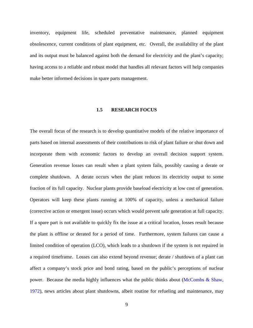
compared to the raw data from the warehouse. Figure 1 shows the cumulative on-hand inventory
and Figure 2 shows an example of raw demand data versus actual demand data for a particular
part. The raw demand data depicts all part demand generated at the plant; this includes parts that
were consumed by the plant as well as parts returned to the warehouse. The actual demand data
depicts only the parts consumed by the plant and not returned to the warehouse. Negative values
in raw demand indicate a return to the warehouse.
The reason the parts were demanded is also central to the spare parts analysis. In general,
parts could be demanded for emergent issues, preventative maintenance, or refueling outage
related work.
Cleansing the data and examining work orders (which showed actual part usage) was
important because of the noise from the high return rate to the warehouse. Once the data was
analyzed, it became apparent that much was hidden in the raw data. Very little actual demand
existed in the historical data, with even fewer urgent corrective actions. The work order and
actual demand analysis showed that only 3.7% of the total demand in the sample set was for
corrective actions, which can place the plant in a compromised state and lead to a plant shutdown
or derate if not immediately remedied. Approximately 30% of demand was for preventative
maintenance work, 9.3% was for refueling outage maintenance, and 57% was for elective and
other maintenance projects that did not compromise plant operations, as depicted in Figure 3.
Clearly, over-ordering exists, with the abundance of false demand signals as evidence of
eventual returns to the warehouse, as shown in both Figure 1 and Figure 2. This excessive
purchasing leads to excess parts in inventory. As a result, using the actual demand data to

18
examine the root cause of the inventory policy currently in use is essential for the development
of any improved policy. Clearly, situations in which the plant might potentially have to shut
down or reduce output are rare. Most parts requests are not urgent but routine, in that lead time
exists to complete the request; those requests can be scheduled and planned for with an improved
ordering process. Examples of non-urgent work include preventative maintenance, elective
maintenance, other maintenance, and some outage maintenance.
On the other hand, given the tremendous costs associated with plant shutdowns or
derates, utility companies cannot simply ignore atypical demand. Rather, they need a better
understanding of costs related to holding and managing inventory and how these costs are related
to the level of risk that deregulated generation companies can tolerate (Scala, Needy, &
Rajgopal, 2009). Such knowledge can lead to better management of costs, tradeoffs, and risk
while maintaining safe plant operations. Thus, triggers of demand and the forecasting process
must be further examined.
Figure 1. Cumulative on hand inventory level for part A
0
1
2
3
4
5
6
7
8
9
5/29/2003 5/29/2004 5/29/2005 5/29/2006
On Hand Inventory Level for Part A
19
Figure 2. Raw demand versus actual demand for part A
Figure 3. Reasons for demand
-4
-2
0
2
4
6
Jan-
03
Apr
-03
Jul-0
3
Oct
-03
Jan-
04
Apr
-04
Jul-0
4
Oct
-04
Jan-
05
Apr
-05
Jul-0
5
Oct
-05
Jan-
06
Apr
-06
Jul-0
6
Oct
-06
Part A Raw Demand
012345
Jan-
03
Apr
-03
Jul-0
3
Oct
-03
Jan-
04
Apr
-04
Jul-0
4
Oct
-04
Jan-
05
Apr
-05
Jul-0
5
Oct
-05
Jan-
06
Apr
-06
Jul-0
6
Oct
-06
Part A Actual Demand

20
2.4 FORECASTING DEMAND
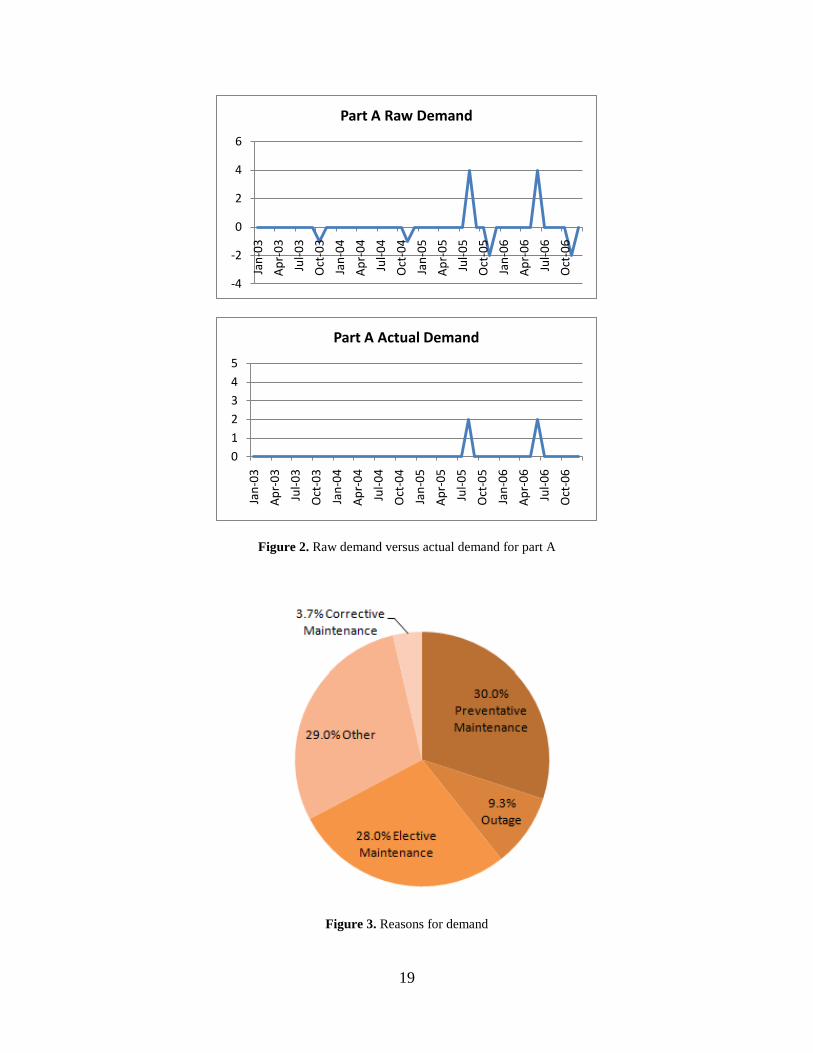
The first step in analyzing the true demand and receipt data was to develop a forecast for parts
requirements. A traditional exponential smoothing forecasting method was first considered for
the raw data. Exponential smoothing is a very popular method and has been one of the standards
in forecasting demands (Willemain, et al., 1994). As will be shown, this approach was rejected
because forecasts lagged behind actual demand due to the intermittent nature of spare parts
demands. Many periods have zero demand, and the forecast and smoothing weights need a
couple of periods to “catch up” to follow demand. The smoothing weight relates the prior
forecast and demand with the forecast for the next period. Thus, zero demands affect the
calculation and reduce the demand value for the next period. Furthermore, the high return rate
skewed the models; traditional exponential smoothing methods typically do not have negative
demands (Wilson & Keating, 2007). Examples of exponential smoothing attempts on the spare
part demands are shown in Figure 4. The first two plots in the figure (part 1 and part 5) plot the
demands by month. The third plot in the figure (part 5) plots the demands by quarter.
Aggregating the demands by quarter versus by month did not improve the forecast, even though
the number of unique periods of zero demand was reduced through aggregation. Furthermore,
accounting for seasonality and / or trend via double exponential smoothing also did not improve
the forecast. These forecasts were obtained via the MINITAB software package. Clearly,
alternate forecasting methods are needed for these data.

21
Figure 4. Exponential smoothing forecast
22
Figure 4 (continued).
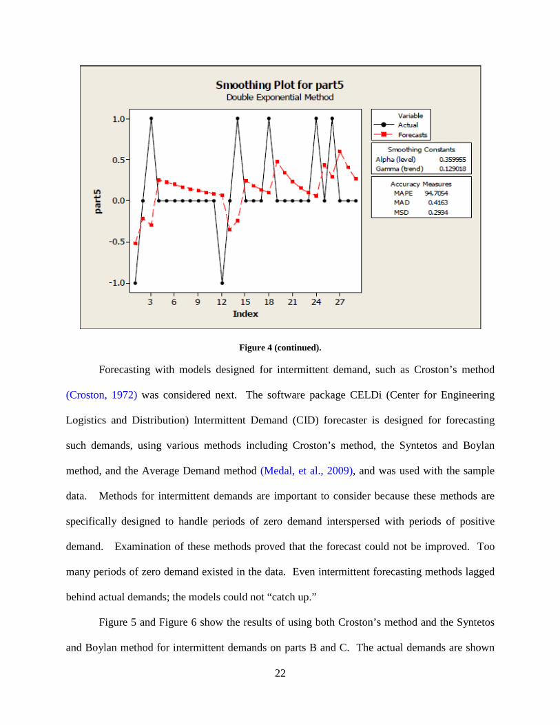
Forecasting with models designed for intermittent demand, such as Croston’s method
(Croston, 1972) was considered next. The software package CELDi (Center for Engineering
Logistics and Distribution) Intermittent Demand (CID) forecaster is designed for forecasting
such demands, using various methods including Croston’s method, the Syntetos and Boylan
method, and the Average Demand method (Medal, et al., 2009), and was used with the sample
data. Methods for intermittent demands are important to consider because these methods are
specifically designed to handle periods of zero demand interspersed with periods of positive
demand. Examination of these methods proved that the forecast could not be improved. Too
many periods of zero demand existed in the data. Even intermittent forecasting methods lagged
behind actual demands; the models could not “catch up.”
Figure 5 and Figure 6 show the results of using both Croston’s method and the Syntetos
and Boylan method for intermittent demands on parts B and C. The actual demands are shown
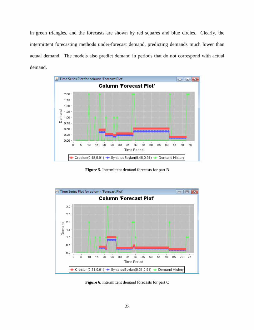
23
in green triangles, and the forecasts are shown by red squares and blue circles. Clearly, the
intermittent forecasting methods under-forecast demand, predicting demands much lower than
actual demand. The models also predict demand in periods that do not correspond with actual
demand.
Figure 5. Intermittent demand forecasts for part B
Figure 6. Intermittent demand forecasts for part C

24
A forecast for demand can also lead to better understanding of equipment failures and
replacements. Beyond demand forecasting, ordering policies and processes can benefit from
better management, especially given the fact that lead times for both planning work and
producing parts in the nuclear power sector can be significant. Understanding the need for parts
during the lead time can help analysts and buyers plan purchases to prevent expediting of and
scrambling for parts if demand should arise during lead time, thus lowering overall purchase
costs. Overall, a clearer understanding of parts usage contributes to identification of
improvement opportunities and promotes improved process management.
While forecasts specify both the timing and quantity of demand, they do not identify the
specific reason for the demand. Elective maintenance, preventative maintenance, and outage
related work can be scheduled and planned. Emergent maintenance involves a failure of a part
that requires immediate attention. Such situations are limited, and even if a forecast could be
calculated, it would be difficult to identify which demands were for emergent or corrective
actions versus demands for non-corrective or routine situations. There are not enough corrective
demands in the data to seed a forecast based on corrective failures alone, and an overall forecast
of all demands would not identify the reason for each demand. Knowledge of failure rates,
component useful lives, and maintenance rules is needed to better predict potential emergent or
corrective actions and corresponding demand. Such specifics can improve the understanding of
failures and potential reasons for parts demand, leading to process efficiency and improved spare
parts management. Failure rates and preventative maintenance (PM) are discussed in the next
section.

25
2.5 FAILURE RATES AND PREVENTATIVE MAINTENANCE
As discussed earlier, the problem of controlling spare parts inventories is complicated by both a
lack of clear supply chain processes at nuclear facilities and a lack of quantitative part data for
forecasting. However, failure rates of plant equipment are not always tracked in the industry,
and there is considerable uncertainty in part demand data, which cannot be quantified accurately.
Component maintenance is not based on the equipment condition (Bond, et al., 2007), and spare
part demands in nuclear generation are highly intermittent. The demands are also stochastic
because part failure is uncertain. PM is scheduled and routine, so demands for PM parts can be
somewhat deterministic. However, while the PM done on parts can reduce the likelihood of a
failure, it cannot prevent all failures. Moreover, the exact extent of the PM work that is needed
for all jobs is not obvious; although a specific PM operation can be scheduled, the corresponding
parts needed may not be known with certainty. To compensate, utilities typically order all parts
that might be needed, contributing to a highly conservative inventory management practice with
heavy over-ordering. Parts that are not used cannot be returned to the vendor, because they are
uniquely made for the plant. As a result, inventory piles up. This heavy over-ordering causes
the plant to return many parts to the warehouse after a PM job is complete.
While a good forecast of demand can improve general ordering policies and processes
related to parts usage, the probability of a corrective issue or part failure should also be
considered. However, failure rates of equipment are not currently tracked with accuracy in the
nuclear industry. The philosophy in the industry is that PM work prevents the failure of
components, and actual failures will not occur. In reality, some failures do occur and can be (1)
emergent, leading to shutdown or derate if not addressed in a specified time frame, or (2)
corrective, fixable at any time. The industry is recently beginning to track failures of some,

26
although not all, equipment. General tracking began as late as 2008 and 2009, so a history of
reliable failure data is not yet available. In a deregulated market, no utility ever wants to be in a
situation where a part fails at an LCO location with no part in inventory to quickly fix the issue,
leading to a plant shutdown or derate with subsequent revenue loss. The cost of keeping critical
parts in inventory versus the potential millions of revenue dollars lost is a tradeoff that favors
keeping additional parts. However, this approach can often result in too many additional parts
and millions of dollars in inventory; that resulting management policy is not efficient, with the
tradeoff possibly no longer favoring additional inventory. Thus, there is a clear need for a
mechanism to determine the importance or criticality of keeping a part in inventory to hedge
against potential revenue loss. Knowledge of failure rates can improve forecasting, especially
those for emergent parts need. The lack of forecasting models and failure rates coupled with
false demand signals lead to high uncertainty regarding which parts are important and how many
to keep on the shelf. Clearly, a new approach to inventory management, demand forecasting,
and ordering policies is needed. This research develops a methodology for identifying critical
parts to store in inventory as well as recommended inventory management policies for those
parts. In order to understand the magnitude of potential exposure to revenue loss in a
deregulated market, cost consequences must be examined.
2.6 COST TRADEOFFS
An analysis of cost consequences helps to identify potential revenue losses if the plant has to be
offlined or derated. These revenue losses are tied to the purchase of replacement power.
Traditional manufacturing firms may delay a shipment in the event of a stockout or offlining of a

27
production line. However, no such option exists in electric utilities, as power demand and
production must be constantly balanced. If demand exceeds production because of the loss of a
baseload electricity plant, it can lead to a blackout in an extreme case, depending on the weather
and the condition of the electric grid. Blackouts are unacceptable and could potentially endanger
customer health. At a minimum, even with no blackouts, the loss of a baseload plant causes
more expensive peaking plants to begin to run in order to replace the power, thus driving up the
hourly cost of power, or locational marginal price (LMP), at the hub where the offlined plant is
connected to the electric grid. Higher LMPs imply higher purchased power costs and more
expensive power for customers, especially those billed on real-time pricing rates. In fact, all
customers would be affected by higher rates if states’ public utility commissions (PUCs) approve
real-time pricing (RTP) for electricity rates. Some cities and states have already adopted RTP
programs, including Georgia, Chicago, New York, and Florida (Borenstein, 2009). Preliminary
research has shown that residential customers would find it difficult to modify their daily
behaviors without incurring large savings on a RTP schedule (Scala, Henteleff, & Rigatti, 2010).
Therefore, higher LMPs could cause even more expense for residential customers.
Generation companies pay a premium to use an alternate source of power. The value of
this power is dependent on grid conditions, transmission congestion, weather, current demand,
time of day, etc. Therefore, the cost of replacement power can vary, but averages have remained
rather steady over recent years. As an illustration, Table 1 shows an analysis of day-ahead LMP
data for PJM Interconnection’s Western Hub (data available from www.pjm.com) from April
2005 to mid-June 2009 with average prices holding steady; the 95% confidence interval limits
that were computed from the data are within approximately one dollar of the averages. The
Western Hub stretches from Erie, PA to Washington, DC. Summer months are June, July, and

28
August. Winter months are December, January, and February. Shoulder months refer to all
remaining months of the year.
Because confidence intervals for costs are tight, companies can use the average values as
a proxy in planning for potential costs of purchased power. The current United States economic
recession has driven power prices lower than average, and as a result, companies today might
incur less of an impact if power is needed. Nonetheless, procuring emergency purchased power
will in general involve a significant amount of resources and revenue loss, regardless of
economic conditions.
Table 1. Day-ahead LMP summary statistics
ONPEAK Summer Winter Shoulder OFFPEAK Summer Winter Shoulder Minimum
LMP $ 27.17 $ 23.62 $ 26.13 Minimum
LMP $ 3.51 $18.99 $ 3.25 Average
LMP $ 83.96 $ 66.59 $ 64.77 Average
LMP $ 49.35 $51.64 $ 43.43 Maximum
LMP $ 369.39 $225.00 $ 199.78 Maximum
LMP $ 256.68 $ 203.31 $160.00 Variance 1791.80 667.58 515.54 Variance 787.90 478.59 361.76 St. Dev. 42.33 25.84 22.71 St. Dev. 28.07 21.88 19.02 Lower 95% CI $ 82.74 $ 65.79 $ 64.30
Lower 95% CI $ 48.59 $51.01 $ 43.06
Upper 95% CI $ 85.17 $ 67.39 $ 65.25
Upper 95% CI $ 50.11 $52.27 $ 43.80
Beyond the factors discussed thus far, risk plays a strong role in spare parts management.
Plant safety is of upmost importance, and the inherent concern of the possibility of a
compromised plant due to a lapse in judgment affects all employee actions. The next section
discusses risk and how its subjective nature can affect decision making. As shown later in this
chapter, plant safety risk is not the proper motivator for spare parts inventory management
decisions; rather, deregulated utilities should be considering risk of revenue loss with respect to
inventory.

29
2.7 SUBJECTIVE RISK AND NUCLEAR POWER
Inherent to this spare parts inventory management problem are the existence of risk and the
related notion of part / component criticality (Scala, Rajgopal, & Needy, 2009). These principles
come into play when predicting which equipment will fail and when it might fail; which spares
parts will be needed in order to repair the equipment; how long it will take to acquire the
necessary parts; how long it will take to complete repairs; and how employees will react to the
situation. Risk and criticality have been widely studied in the literature; here we focus on the
energy industry, particularly the nuclear sector. Research shows that employees and their
perceptions of risk as well as external (public) perceptions of risk play a major role in policy
development. Consequently, their inputs are critical elements in managing overall policy.
Background material on this subject is reviewed next.
2.7.1 Risk
Risk is inherently subjective and socially construed (Slovic, 1999; Thomas, 1981).
Furthermore, risk involves unacceptable consequences with very high costs that no entity wants
to pay; this distinguishes it from traditional cost-benefit analysis (Saaty, 1987). There are two
major components to risk. The first is the personal risk that employees perceive to themselves
and the facility at which they work. This risk obviously plays a role in spare parts management;
ultimately, it is the employees who make the decisions to perform maintenance work, buy parts,
and set part stocking levels. How they perceive the effects of their decisions in these areas
influences the decisions that they make and ultimately affects the spare parts inventory at the
facility. The second major component is general public perceptions of risk, which also plays a

30
role in spare parts management. In particular, in nuclear plant operations, the nature of nuclear
power and how people perceive it lead to extra diligence to prevent any plant issue, no matter
how minor. This in turn leads to a large reliance on the insurance provided by having spare parts
on hand. The following subsections address these two aspects of risk—personal and public—in
more detail.
2.7.2 Employee Level of Risk
The first area of risk involves employees and the outcomes of their behaviors and decisions.
Employees can have great autonomy in making inventory control decisions such as stocking
levels, SKUs to order, order quantities and order / delivery dates. Each action yields a buy / no
buy decision that ultimately affects inventory levels and policies for spare parts management.
Spare parts can be especially crucial in the nuclear power industry; in a worst case scenario, the
lack of availability of a part can lead to a plant derate or shutdown. Therefore, it is essential that
employee behaviors relevant to perceived risk be factored into spare parts ordering policies for
electric utilities, because actions of power plant employees have consequences related to the
actual risk to which they are exposed (Sjöberg & Sjöberg, 1991). Clearly, both under and over
estimations of risk can have negative effects (Sjöberg & Sjöberg, 1991).
Perceptions of risk in the power sector have not been extensively studied from a rigorous,
research perspective (Sjöberg & Sjöberg, 1991; Kivimäki & Kalimo, 1993). Three relevant
papers that have examined the perceptions and behaviors of employees in the nuclear sector are
Sjöberg and Sjöberg (1991), Kivimäki and Kalimo (1993), and Kivimäki, Kalimo, and Salminen
(1995). Sjöberg and Sjöberg (1991) examined both risk attitudes and risk assessments in nuclear
power workers and their connections to radiation and related risks. As part of this study, the

31
authors examined the effects of personality and job function as well as the relationship between
risk perceptions and job satisfaction. They looked at a large sample of employees, mainly at the
maintenance level, through semi-structured interviews and a follow-up survey. Such techniques
were chosen because the authors argued that standard procedures for assessment did not exist.
The results showed that risk perceptions varied depending on the different definitions that
employees gave to risk. These definitions were not dependent on work group, but differences
were apparent based on exposure to controlled areas (i.e., protected areas of high radiation where
a special suit is required to be worn to enter the area; United States federal guidelines limit the
exposure to radiation per year (NRC, 2010)).
Sjöberg and Sjöberg (1991) also found that employees with weak self-confidence and
high anxiety judged job risks to be higher than other groups. Furthermore, an inverse-U
relationship exists between risk of general accidents and job risk. Employees who perceive job
related and nuclear risks to be low also rank other, more general risks to be low. On the other
hand, employees who perceive job related and nuclear risks to be high and are more anxious also
rank other, more general risks to be low because these risks do not seem to be as significant as
nuclear related risks. A plot of these perceptions, with perceived job risk on the x-axis and
perceived general accident risk on the y-axis, thus takes an inverted-U shape. Figure 7 shows an
illustrative adaptation of the graph in Sjöberg and Sjöberg (1991).
Kivimäki and Kalimo (1993) examined risk perceptions of nuclear workers in
comparison to workers in non-nuclear and power industries as well as the relationship between
risk attitudes and well-being / organizational commitment. The authors administered a Likert
based survey at a nuclear plant in Finland and found that perceptions of an accident were
strongly related to organizational commitment and slightly related to job satisfaction. The

32
authors note that it is essential to recognize which attitudes affect performance, as errors can
have large negative consequences.
Figure 7. Adaptation of general job and accident risk graph (Sjöberg & Sjöberg, 1991)
Kivimäki, Kalimo, and Salminen (1995) extend the results in Kivimäki and Kalimo
(1993) in a second paper that examines safety perceptions and the relationship with
organizational commitment (OC) and its components: OC-acceptance, OC-willingness, and OC-
desire. OC-acceptance is traditionally defined as acceptance of the organization’s goals and
values; OC-willingness is the willingness to put forth effort on the organization’s behalf; OC-
desire is the desire to remain with the organization (Kivimäki, Kalimo, & Salminen, 1995). The
authors argue that senior management must constantly balance safety and financial goals with
owners as well as regulatory, economic and public stakeholders. The authors propose that
employees who do not agree with or trust the balance between safety and economic goals will
judge risk to be higher. They found a correlation between OC-acceptance and appraisals, or
employees’ perceptions of the effectiveness and competence of top management. They also
found the correlation between perceptions of risk and OC-acceptance to be lower and the
correlation between perceived risk and OC-desire to be higher among managers. Such a result
suggests the existence of two cultures in the organization—one comprised of management and

33
another of traditional employees. These cultures have differing views of perceived nuclear risk,
OC-acceptance, and OC-desire. As a result, managers must lead a group of employees who may
have differing views of the organization and values. Managers are important in promoting a safe
environment, especially because Kivimäki, Kalimo, and Salminen (1995) found a strong link
between perceived nuclear risk and appraisals of management. This result is especially
important because this research proposes that managers currently play a large influential role in
promoting a risk averse (and therefore high) safety culture. Such a culture can greatly impact the
spare parts ordering policy in effect at a utility.
In summary, the scholarly literature of risk in the nuclear industry shows that employees
and their perceptions play a significant role in managing the work environment. In a
complicated system such as spare parts management, with lots of inputs and decision makers,
this therefore suggests that employees play a major role in policy implementation.
Consequently, their perceptions and behaviors are important to understand and capture for
overall policy development, as this factor has been relatively underrepresented in research.
While the above studies do not specifically address spare parts, the possibility of a
nuclear accident can be paralleled to the possibility of an undesirable, compromised situation
arising from a part failure and spare parts stockout. Nuclear energy has a work subculture that is
consistent among utilities, so it is possible to extend the results established for the European
plants to those in the United States. Results regarding behaviors such as managerial influence,
risk perception, and attitudes are relevant to consider in building a dynamic and robust spare
parts inventory management policy. Therefore, a need exists to extend these findings to spare
parts inventory and validate relevant concepts for United States nuclear facilities.

34
2.7.3 Public Perceptions of Risk
Nuclear energy plants have safety cultures, which Harvey, et al. (2001) cite as having no clear
definition, but nonetheless constituting a key predictor of safety performance. The objective of
safety is paramount in the nuclear industry; currently it consistently takes precedence over the
business bottom line in decision making. Kivimäki and Kalimo (1993) propose that nuclear
organizational commitment may improve production safety and reduce the probability of a
serious accident. Yule, Flin, and Murdy (2007) cite a study where worker perceptions of
management commitment to safety were associated with low accident rates. However, public
perceptions with respect to safety are different from those of workers and are often unrelated to
both the inspection certifications from the United States Nuclear Regulatory Commission (NRC)
and demonstrated safe operation of plants.
Historically, the general public perceives nuclear energy to be more risky than other
forms of energy production. Mullet, et al.’s (1998) study of eighty university students found that
the students ranked nuclear energy to be the most risky—regardless of the production process—
when compared to eight other forms of energy, namely wood and biomass, coal, gas, oil, water,
wind, geothermal, and solar. The lowest risk rankings were attributed to wood, coal, and solar
technologies. Mullet, et al. (1998) also cite multiple studies that rate nuclear power as having
high risk; in particular, ten of thirteen reviewed studies found nuclear to be the highest in terms
of risk. Thomas (1981) conducted a survey in Austria regarding public perceptions of the risk
and benefits of energy. The author found that respondents who were against nuclear energy
perceived it to lead to various risks, namely environmental risk, indirect (future and political)
risk, and psychological and physical risk. The beliefs of the public were found to be
underestimated by a control group of policy makers and experts on nuclear power. The results

35
reflect the argument put forth by Slovic (1999) that the public has a broad conception of risk and
experts’ risk perceptions are not related to the underlying dimensions of risk. Furthermore, risk
conflicts result from conceptual differences between the public and experts. Slovic (1999)
argues that experts and the public disagree because both groups have different definitions of risk,
worldviews, affective experiences / reactions, and social status. This dichotomy breeds a culture
of distrust, causing the public to reject experts’ risk assessments (Slovic, 1999).
Even small issues and situations at a plant feed into the public’s perception of nuclear
energy. Slovic (1999) argues that distrust exists between the public, industry, and risk
management experts. As a result, the public may perceive that small, routine plant issues are
actually more serious than what is reported by the company. Furthermore, the trust between the
public and industry is easily destroyed in that negative events are more salient and carry more
weight than positive events. Such events need little credibility to be considered true, and, once
distrust begins, it tends to be reinforced and perpetuated (Slovic, 1999). For events with extreme
negative consequences, the possibility of such an event becomes salient, and small probabilities
have great weight in people’s perceptions (Slovic, et al., 2004). Furthermore, the public is often
difficult to educate on scientific concepts and facts (Sjöberg & Sjöberg, 1991), and risk and
benefit become negatively correlated in their minds (Slovic, et al., 2004).
In general, employees might not perceive a situation to be as risky as the general public.
In particular, nuclear personnel do not perceive nuclear risk to be a serious problem when
compared to the public (Kivimäki, Kalimo, & Salminen, 1995). Kivimäki and Kalimo’s (1993)
study found that plant workers estimated less likelihood of a serious accident and felt that plant
safety was better when compared to a random sample of the Finnish population. However, even
among employees, two safety cultures exist. Yule, Flin, and Murdy (2007) found that

36
perceptions of supervisors and management influence perceptions of commitment of senior
managers by employees and argue that supervisors can have a negative impact on the safety
climate by applying too much pressure on workers. Harvey, et al. (2001) argue that the safety
culture is conceptually different for various groups of workers, especially between managers and
shop floor employees. Furthermore, the authors cite that accidents can result from the existence
of two separate cultures and that latent organizational failures will always drive actual individual
errors (Harvey, et al., 2001).
Translating these ideas to spare parts, it becomes evident that lapses in ordering judgment
by employees are probably indicative of a poor inventory management policy enacted by the
company and / or a lack of understanding of the entire ordering process and its corporate and
operational impacts by the employee. This misunderstanding or error may also stem from the
employee’s dedication to the nuclear safety culture without concern for the company’s overall
bottom line and sustainability. In an extreme case, the absence of a spare part when needed for
equipment breakdown may lead to a compromised plant, so considering both public and
employee perceptions of nuclear safety is important when developing a sustainable spare parts
inventory management policy (Scala, Rajgopal, & Needy, 2009). Nuclear accidents have high
consequences but low probability of actually occurring, given that appropriate practices and
NRC guidelines are followed in the plant. In summary, no one wants a nuclear plant meltdown
or near-miss, and this extreme outcome feeds into the spare parts ordering policies. Furthermore,
the business’ bottom line was ignored under regulation because monetary return for relevant
operating expenditures, including spare parts, was guaranteed. This mentality carries over into
current policies and is coupled with very high risk averseness to maintain safety.

37
However, risk is not limited to perception. Due to the high costs of replacement power,
risk of revenue loss in a deregulated market is significant. The next section discusses this risk
and why it should be considered the prevalent risk in spare parts inventory management
decisions.
2.8 RISK OF REVENUE LOSS
Overall, as discussed, purchased power costs tend to be much more substantial than the costs of
carrying inventory, once part lead time and repair time are factored in. However, few part
demands are tied to a compromised situation where plant output can be reduced. More
importantly, even though generation companies might generally believe that spare parts
inventory is protecting plant safety, in reality, the inventory covers the risk of a revenue loss.
The idea that spare parts protect plant safety is tied to the employee and management perceptions
of risk outlined in the previous section. Nuclear generation plants must be operated safely to
maintain NRC approval and remain in operation. The NRC monitors safety at the United States
nuclear plants and approves both applications and renewals for plant operating licenses. Many
automatic controls are in place to shut down the entire plant without human intervention in the
event of a compromised situation. The probability of a catastrophic situation is extremely low,
and the controls help to prevent an accident. Therefore, in essence, holding inventory covers the
risk of revenue loss from offlining the plant. Elective maintenance, preventative maintenance,
and outage related work can be scheduled with parts arriving just-in-time. Inventory would only
need to be held to hedge against a corrective action requiring immediate attention. Plant safety is
not singlehandedly or directly tied to spare parts inventory.

38
Considering spare parts management at generation plants, especially nuclear plants, in
terms of revenue loss is to our knowledge a new concept. Under regulation, costs of doing
business were recovered in customers’ electricity rates; optimally managing costs were not of
particular concern, especially in the name of safe plant operations. However, plant safety is not
purely dependent on spare parts held in inventory, which seems more tied to keeping the plant
fully operational. Understandably, generation companies prefer to keep nuclear plants running
once synched to the electric grid because the marginal operating costs of the plants are relatively
low, compared to the LMP prices at which the power can be sold. These plants return a large
profit, especially because approximately 20% of U.S. electricity is generated through the use of
nuclear power (US EIA, 2010). Companies prefer to reduce power only for refueling outages, as
long as safe operations are maintained. Nuclear power itself is inexpensive to generate, but
plants have high capital costs.
However, a better business plan may allow for the possibility of some small derates or
power reductions to conserve capital and dollars currently tied up in spare parts inventory. At a
minimum, companies need to refresh their thinking about operations in a deregulated
environment versus the cost-covering regulated environment. This research addresses these
issues and opportunities. Allowing deregulated utilities to understand their cost tradeoffs with
respect to spare parts will enable them to institute better processes and policies for spare parts
management, enabling them to become more efficient, more cost-conscious, and better
engineered to fit their operating and business environment, while maintaining company and
shareholder expectations. The methodology developed in this research addresses these
opportunities.

39
2.9 FOUR STEP METHODOLOGY
This research takes an engineering management approach to spare parts inventory management.
Such an approach focuses on practice and eliminates the need for theoretical or impractical
assumptions in mathematical models while incorporating all relevant factors and forces in the
process. As discussed, demand for spare parts cannot be accurately forecasted, and part failure
rates are not readily available. Deregulation changes the game, as generation facilities must
operate as competitive businesses with no guarantee of cost recovery. Furthermore, based on the
company being used as a test bed for this research, it is clear that the nuclear industry is not
methodical about its current spare parts processes. This research will balance the risk of revenue
loss through a part scoring system that rates the importance of keeping an individual part in
inventory. This scoring system and corresponding inventory stocking policy recommendations
are achieved through a four step methodology:
1. Development of an influence diagram of the spare parts process
2. Use of the Analytic Hierarchy Process (AHP) to rank influences
3. Development of a part criticality scoring system for spare parts
4. Construction of inventory policies based on retrospective simulations
The influence diagram maps out the current spare parts process and identifies all
influences that are relevant to the process. The diagram depicts all factors and forces in the
problem and provides a clear picture of the as-is process. Spare parts are more than just a supply
chain problem, and the diagram allows for input from all plant departments, such as
maintenance, planning, supply chain, etc. Furthermore, continuous improvement can only result
from a clear understanding of the as-is process. The influence diagram captures knowledge of
the process as a basis for continuous improvement and helps to discern the process issues

40
associated with returns to the warehouse. Further details of the influence diagram and its
development are provided in Chapter 3.
The second step of the methodology is to rank the influences on the diagram. This is
achieved through group decision making in the AHP. Nuclear industry experts from various
departments and work functions made individual pairwise comparisons of the influences on the
diagram, and those comparisons are aggregated into a single judgment for AHP prioritization.
AHP is chosen for aggregation and weighting of the influences because it is an accessible
method that employees can easily understand and participate in, even if they have limited
technical backgrounds. Furthermore, the AHP captures employee knowledge through the
pairwise comparisons. With a significant portion of the experienced workforce due to retire in
the near future, capturing their extensive knowledge of the process is not only important but also
can be invaluable to the industry. The interview protocol and AHP hierarchy information is
detailed in Chapter 4. In implementing the AHP, challenges were encountered in group
aggregation, and a new method is developed for group aggregation when the criterion from the
Saaty and Vargas (2007) dispersion test is violated and the decision makers are unwilling or
unable to revise their judgments. This method is detailed in Chapter 5 along with a discussion of
the dispersion test.
The third step of the methodology is to develop inventory criticality scores for each spare
part. Inventory criticality refers to the importance or criticality of keeping a part on hand in
inventory. Inventory criticality should not be confused with engineering criticality, which is a
standard nuclear industry classification of part usage and corresponding maintenance schedule.
These inventory criticality scores are built from the AHP prioritization weights and historical
part data. Higher scores imply greater criticality. Parts are then placed into three natural groups

41
for inventory management based on score. Addressing parts from a management perspective can
improve the current industry policies and practices by providing an understanding of how parts
can affect the company bottom line. Further details regarding the scoring process are given in
Chapter 6.
Finally, a base stock inventory policy is developed for each part group through
retrospective historical simulation. Results from the retrospective simulations lead to tradeoffs
between cost of base stock inventory and average delayed work days per part per month.
Feedback from the test bed company will allow for determination of the best policy. The
methodology and corresponding polices presented are not prescriptive but rather a guideline,
where companies can trade off the appropriate risk of delaying work versus the capital cost of
inventory, based on their own risk averseness. Determining the important parts helps to buffer
the risk of revenue loss associated with plant derate or shutdown, which results from an emergent
situation that compromises the plant with parts not immediately available to remedy the issue.
Further details regarding the simulation are given in Chapter 7.
Overall, the methodology presented in this dissertation can be generalized to other
industries and companies experiencing difficulty in managing their intermittent spare parts
demands. Appropriate modifications to the process influence diagram can be made for other
nuclear plants and deregulated electric utilities. Furthermore, companies can use the
methodology in total or just individual parts of it to develop their own influence diagram, AHP
prioritized weights, criticality scores, and / or corresponding inventory policies. This dissertation
details the methodology for the nuclear electricity generation industry, utilizing data from a test
bed company for illustration. The applicability is not limited to this one instance; rather the
work can be readily generalized so that all other industries with intermittent spare parts demands

42
can apply the four step methodology to improve their inventory management. The next chapter
discusses the development of the influence diagram, which is the first step in the methodology.

43
3.0 INFLUENCE DIAGRAM
3.1 BACKGROUND
An influence diagram is a pictorial representation of a decision problem. All relevant factors and
forces, both quantitative and qualitative, are depicted in one single figure. Variables that are
stochastic or have an element of chance are represented typically by circles or ovals, while
variables that are decisions and can be controlled by the decision maker are represented by
rectangles or square boxes. Relationships between variables are depicted by arcs, with a directed
arc from block A to block B implying that item A influences item B. A connection between
blocks is not necessarily causal. See Figure 8 for an example of the nodes on an influence
diagram.
Figure 8. Influence diagram node example
Influence diagrams allow people with limited understanding of the overall process or with
limited technical backgrounds to better understand the process and inputs to the decision
problem. They can be developed as a collaborative effort between a decision maker and an
analyst. For a detailed discussion of the theory of influence diagrams, see Howard and Matheson

44
(2005). A discussion on probabilistic elements of influence diagrams and their analysis through
the use of computer algorithms is given in Shachter (1986; 1988).
3.1.1 Examples of Use of Influence Diagrams
Influence diagrams are commonly used to map out problem variables and the relationships
between the variables. Examples of the use of influence diagrams are varied and include pitcher
substitution in Major League Baseball (Scala, 2008), risk management and policy options post-
eradication of the polio virus (Duintjer-Tebbens, et al., 2008), testing strategies for
pharmaceutical drug candidates (Keefer, 2004), evaluation of military alternatives for countering
weapons of mass destruction (Stafira, Parnell, & Moore, 1997), maritime risk assessment and
decision support (Eleye-Datubo, et al., 2006), infection risk communication in plague
bioterrorism attacks (Casman & Fischhoff, 2008), modeling classroom newsvendor problems
(Pfeifer, et al., 2001), diagnostic testing in manufacturing (Agogino, et al., 1992), and safety
assessments of products containing nanoparticles (Morgan, 2005).
3.2 MODELING THE SPARE PARTS PROCESS IN NUCLEAR PLANTS
An influence diagram was chosen for several reasons to depict the current inputs to the spare
parts process. An influence diagram clearly depicts all factors and forces in the problem,
allowing the problem analysts and decision makers to see all elements that affect the overall
decision problem, in this case spare parts inventory. The relationships between these elements

45
are also clearly depicted, allowing the subject matter experts and decision makers to take a step
back from their experiences with respect to the day-to-day process and digest the overall spare
parts inventory problem. The analysts and subject matter experts may not clearly understand the
full ramifications of their decisions and the problem itself, and an influence diagram allows for a
pictorial representation of the problem in a format that provides insights into both the details of
the problem and its overall effects (Scala, Rajgopal, & Needy, 2010). The majority of the
individuals worked with at the test bed company have little decision modeling experience and
some also have limited technical backgrounds. The influence diagram allows them to easily
understand the problem so that they can initiate process improvement, as well as to easily
validate or verify the structure of the diagram based on their work experiences and knowledge.
The influences form a basis to consider the problem beyond traditional supply chain concepts.
The considerations and thought process by every group that makes spare parts decisions in the
plant are represented in the influence diagram.
Because an influence diagram has been proven in the literature to be effective at
depicting decision problems (see examples noted above), other companies and industries
implementing the methodology developed in this dissertation can easily adapt the diagram to fit
their own inventory modeling process and decision needs. The following is a discussion of the
rationale for the influences that were included in the diagram developed in this research.
3.3 INFLUENCE DIAGRAM MODEL
The overall structure of the influence diagram for spare parts in nuclear plants places influences
in groups based on both categorical and company process characteristics. To develop the

46
diagram, the expertise of various work groups at the test bed company was employed. These
groups included supply chain, planning and scheduling, engineering, equipment reliability,
maintenance, work management, outage management, and asset utilization. These experts also
assisted with model validation. In particular, the nuclear spare parts problem is complicated and
affected by more than just the actions of a plant’s supply chain department. The plant’s planning
department plans the maintenance work and generates a list of parts. This list is influenced by
maintenance schedules, vendor availability, scope of work, etc. The complexity of the problem
quickly becomes clear when building an influence diagram. All plant departments that affect
spare parts decision making must be represented on the diagram through identification and
mapping of all relevant spare parts influences, and everything that affects spare parts
management must be represented on one diagram. Once all the factors, forces, and inputs to the
process are depicted, the decision maker can start to identify important relationships and
opportunities for continuous improvement.
The influence diagram was developed as a collaborative effort with the employees at the
test bed nuclear generation facility. These employees provided feedback to the model, adding
and removing influences as appropriate. This process was iterative and allowed for full
discussion of the spare parts problem’s decision making environment. Also, the diagram
development process allowed plant employees, some without technical experience and decision
making backgrounds, to easily participate in the process and contribute vital information. As
more information was collected from the employees who work with and make spare parts
decisions every day, the diagram became more complete, fully revealing the decision making
environment, along with its complexities. As discussed previously, the lack of detailed and
complete part data coupled with highly intermittent demands lead to high uncertainty regarding

47
the best way to manage the nuclear spare parts process. The influence diagram reduces this
uncertainty by visually depicting the decision making environment and providing a basis for
improving the inventory management process.
To aid in the process of collecting both information and employee expertise, influences
were grouped into sets. Each set contained all influences that corresponded to a given plant
department or specific technical knowledge area. As one example, influences related to the
expertise of the planning department were placed into a single set. These common
characteristics led to seven sets of influences, namely (1) Timeliness of Work Order, (2) Part
Failure, (3) Vendor Availability, (4) Part Usage in Plant, (5) Preventative Maintenance Schedule,
(6) Outage Usage, and (7) Cost Consequences.
Each set of influences focused on a common theme. For example, all influences in the
“Vendor Availability” set were related to supply chain activities. All influences on the diagram
that were part of the supply chain function were placed in this set. Therefore, an employee in the
supply chain department should be familiar with the influences in that set and able to accurately
judge the relative importance of each influence in that set. Overall, for each set of influences,
insight regarding how the influences affect spare parts inventory management and ordering
decisions can be gained from the relative importance rankings between the influences in the set.
Figure 9 depicts the high level diagram of the overall set of influences and their effects on
determining a part score and subsequently the criticality index of a part. Table 2 depicts the
influences contained within each set; each of these sets leads to a sub-diagram. As an
illustration, the sub-diagram for the “Timeliness of Work Order” set is included in the bottom
half of Figure 9 which also depicts how this sub-diagram connects to the high level diagram.
Other sets have their own influences (as detailed in Table 2) and lead to their own sub-diagrams
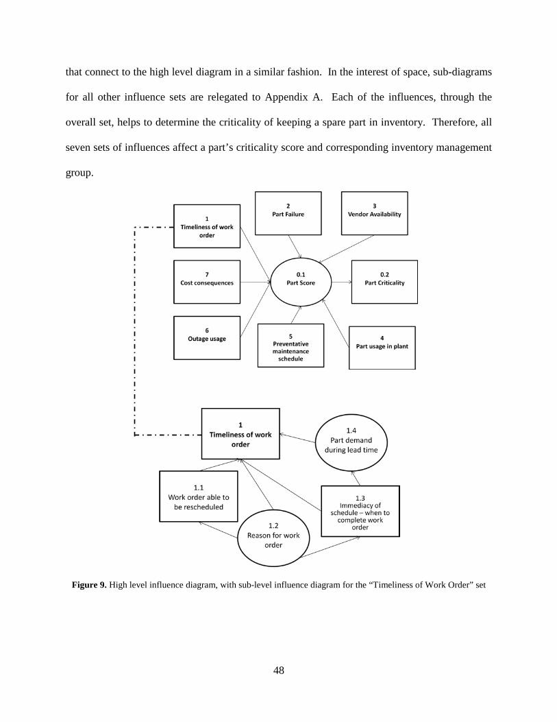
48
that connect to the high level diagram in a similar fashion. In the interest of space, sub-diagrams
for all other influence sets are relegated to Appendix A. Each of the influences, through the
overall set, helps to determine the criticality of keeping a spare part in inventory. Therefore, all
seven sets of influences affect a part’s criticality score and corresponding inventory management
group.
Figure 9. High level influence diagram, with sub-level influence diagram for the “Timeliness of Work Order” set

49
Table 2. Influences in the spare parts ordering process along with node connections
Item Description Connects
to Item Description Connects
to 0.1 Part score 0.2 4 Part Usage in Plant 0.1
0.2 Part criticality n/a 4.1 Part is at a single point vulnerability 4
1 Timeliness of Work Order 0.1 4.2 Installation in a functional location tied to LCO 4
1.1 Work order able to be rescheduled 1 4.3
Usage for equipment train protection and reliability 4
1.2 Reason for work order 1; 1.1; 1.3 4.4 Number of locations in plant where part installed 4
1.3 Immediacy of schedule—when to complete work order 1; 1.4 4.5
Regulatory requirement to keep part on-hand 4
1.4 Part demand during lead time 1 4.6 Usage to prevent equipment forced outage 4
2 Part Failure 0.1 4.7 Open work orders and part demand 4; 1.5
2.1 Failure of part leads to LCO or SPV 2 4.8
If the part requested is actually used in the PM work order 4
2.2 Lab testing results in predictive maintenance 2 5
Preventative Maintenance (PM) Schedule 0.1
2.3 Surveillance maintenance results 2 5.1
PM done on the related equipment 5
2.4 Failure history 2 5.2
Frequency of time the actual PM job is more involved than anticipated 5
2.5 System health for related equipment 2 5.3
PM done online or only during outage 5
2.6 Normal part life 2 5.4 Associated maintenance rules for the equipment 5
3 Vendor Availability 0.1 6 Outage Usage 0.1
3.1 Vendor discontinued or obsolete 3 6.1
Part scheduled for use during outage 6; 6.2
3.2 History of vendor quality issues 3; 3.3 6.2
Actual usage of the part during outage 6
3.3 Vendor reliability 3 6.3 When the part can be used or equipment accessed 6
3.4 Vendor lead time 3; 3.3 7 Cost Consequences 0.1 3.5 Availability on RAPID 3 7.1 Cost of expediting the part 7
3.6 Quality testing or hold before installation 3 7.2 Cost of replacement power 7
3.7 Ability to expedite the part 3
50
In practice, such a breakdown of the model into sub-diagrams is common so as to
simplify visual representation without losing any relevant information while also allowing the
decision maker to effectively digest the information presented. An example of the use of sub-
diagrams can be found in Agogino, et al. (1992). In general, items selected as influences are
based on studying the system and interviewing key process stakeholders. For the spare parts
inventory process, industry experts in the supply chain area at the test bed company reviewed
and validated the diagram’s influences and relationships (Scala, Rajgopal, & Needy, 2010).
During the review, some influences were reassigned to different influence sets, based on the
experts’ expertise and knowledge associated with their work function. The items on the diagram
were also further validated against various internal documents as well as industry standards,
including the Nuclear Energy Institute’s “AP-908: Materials Services Process Description and
Guide” (NEI, 2008). Each set of influences supports the overall inventory decisions of what to
buy, when to buy, what to store, and how much to store. Decisions are typically made after a
work order is generated or a reorder point is reached, in an effort to maintain plant safety and to
comply with federal regulations. Descriptions of the diagram sets are detailed in the following
section and are summarized in Table 3.
3.3.1 Influence Set Descriptions
1. “Timeliness of Work Order” refers to the influences that are related to both when the
work order can be completed and the associated parts that would be required to finish the work
order. Each influence supports the work order process and the immediacy of completing the
needed plant maintenance as well as associated part demand and work order characteristics,
requirements, and criticality.

51
Table 3. Summary of influence sets
Influence Set Description
1. Timeliness of Work Order Work order completion and associated parts 2. Part Failure Indicators to predict failure 3. Vendor Availability Parts supply and procurement 4. Part Usage in Plant Installation and use in the plant 5. Preventative Maintenance (PM) Schedule Activities and parts associated with PM 6. Outage usage Activities associated with outage maintenance 7. Cost consequences System-wide costs to derate or offline plant
2. “Part Failure” refers to the influences that are indicators of imminent or future part
failure. Such part failures may place the plant in a compromised situation. This includes the
possibility of a limited condition of operation (LCO), where the plant personnel have a specified
amount of time (usually 72 hours) to remedy the situation or shutdown / derate the plant
according to federal mandate. The test bed company has internal labs that test both plant
equipment and chemistry to support proper and safe plant performance along with a system to
track some failure history. Surveillance maintenance involves visually inspecting components
for defects or needed maintenance. System health involves an internal quarterly score given to
plant systems based on various operational factors.
3. “Vendor Availability” refers to the influences that represent the ability of vendors to
supply spare parts when needed and the ease with which parts can be procured. In particular,
RAPID is a database unique to the nuclear industry where nuclear plants can purchase or borrow
needed spare parts from other utilities. Quality testing refers to appraisal testing that must be
completed before the part can be installed in the plant.
4. “Part Usage in the Plant” captures the influences that represent the volume and frequency
with which a spare part is installed or used in the plant. Functional locations are codes referring

52
to physical locations where parts are installed in the plant. Train protection (measures to ensure
the safety of the plant’s two production trains, denoted A and B) and equipment forced outage
(EFOR) refer to keeping the plant safely running and preventing equipment from being offlined.
Single point vulnerability (SPV) means only one component of a given type is installed in the
plant; no backup system exists in the event of failure.
5. “Preventative Maintenance (PM) Schedule” refers to influences that represent activities
associated with PM, corresponding maintenance rules, and how parts are selected to be included
on a PM work order. Each influence within this set is directly related to the PM policies and
related plant work.
6. “Outage Use” refers to influences that capture information related to parts requested for
use during a plant outage and when the related work orders can be carried out. Each influence
within this set is directly related to work that must be or is typically done during a scheduled
plant refueling outage, which occurs every eighteen to twenty-four months, depending on the
plant.
7. “Cost Consequences” refers to the influences that represent company-wide costs incurred
if the plant has to be offlined or derated, particularly without prior notice, in a forced outage
situation. Each influence within this set supports related costs incurred if a part is not available
when required, thus causing the work to not be completed and the nuclear plant to be offlined or
derated.
Each set contains characteristics that are similar to each other, and all sets taken together
fully describe the nuclear spare parts process. In order to calculate criticality scores for each
spare part, the influences must be quantified in some manner. Because the influences are placed
in sets, industry experts with knowledge of a set will be familiar with all influences in that set.

53
Those experts could appropriately understand and discern the influences in that set and provide
judgment of relative importance of the influences in that set.
3.4 JUDGEMENT OF INFLUENCES
Because we are considering relevant influences across work groups, group judgments of the
influences on the diagram are needed. Employee knowledge is a crucial component of the
model; one employee’s perspective is simply not enough for knowledge representation and
robust decision making. Employees have limited overall plant knowledge but detailed
experience within their work groups. Spare parts management is a system-level problem
throughout the entire plant and is not isolated to one group. Varied information from multiple
employees and work groups is needed to represent what is really happening in the process (Scala,
Needy, & Rajgopal, 2010). Furthermore, incorporating the perspectives of many employees in
various work groups also helps to record the employees’ undocumented knowledge accumulated
over years of work experience to ensure that once employees retire and leave the company, the
corresponding spare parts knowledge will not be lost.
The Analytic Hierarchy Process (AHP) is an excellent way to capture and synthesize
qualitative knowledge from individuals and even from a group. The AHP is a decision tool
developed by Thomas Saaty (1980). It supports decision making by synthesizing pairwise
comparisons of decision attributes across alternatives and calculating priorities (Saaty, 1980;
1990). Because the model involves pairwise comparisons, qualitative items can be compared,
judged, and ranked. This feature lends itself to spare parts management and process influences
as quantitative failure data does not exist and not all influences on the diagram are easily
54
quantifiable. Most influences represent qualitative concepts and subjective decision making.
Overall, the AHP supports both an engineering management approach to spare parts and the
integration of the process among multiple work groups at a nuclear plant, demonstrating the
effects of decision making beyond the typical supply chain and plant maintenance groups.
3.5 VALIDATION
The influence diagram was developed as through an iterative process with the SMEs at the
nuclear power generation test bed facility. A list of possible, observed influences to the process
was defined and presented to the SMEs who removed non-relevant influences and added others.
The influences were then placed into sets, with the SMEs verifying the sets so that all influences
associated with a particular knowledge area were placed into a single set. This process of
influence definition and placement into sets was repeated until all SMEs could agree with the
process influence list and corresponding set placements. Discussions with the SMEs took place
via conference calls and email correspondence. A total of five SMEs participated in the
validation of the influence diagram; four of the SMEs held supervisory or managerial positions.
In sum, the influence diagram was developed to frame the problem. The process
produced a list of factors categorized appropriately for application of the Analytic Hierarchy
Process (AHP) and prepared the SMEs to properly complete the pairwise comparisons required
in the AHP. The influence diagram is an as-is model of the nuclear spare parts management
process at the test bed facility; creation of the diagram opened a dialogue about the process that
led to justification of the important factors in the process. The diagram depicted the relationship

55
between the influences, and based on the relationships, the relevant pairwise comparisons could
be completed.
3.6 SUMMARY
This chapter developed an influence diagram for the nuclear spare parts process and
presented the influences in seven sets. Relationships between the influences and sets are clearly
depicted, providing clarity to the current process and an understanding of how various factors
and forces affect each other. To our knowledge, an influence diagram of the nuclear spare parts
process has not been previously developed or presented in literature. The influence diagram is a
tool that is helpful to discern the current spare parts process and categorize it into sets for the
AHP analysis. The next chapter discusses the use of the AHP to synthesize the influences to the
nuclear spare parts process.

56
4.0 INTERVIEW PROTOCOL AND USE OF THE ANALYTIC HIERARCHY
PROCESS (AHP)
4.1 BACKGROUND ON THE AHP
The main construction of the Analytic Hierarchy Process (AHP) is a hierarchy with the goal of
the analysis at the top, a listing of decision attributes in the middle tiers, and a bottom tier of
decision alternatives. Pairwise comparisons between each set of alternatives or attributes on the
level below are made with respect to the attributes in the next higher level. For example, if a
problem has three attributes and five alternatives, a set of pairwise comparisons between all five
alternatives would be done three times: once with respect to each attribute. A set of pairwise
comparisons of all attributes with respect to the goal would also be done. Pairwise comparisons
involve selecting which item is more important with respect to the attribute in question and then
stating how much more important the item is over the other item in terms of a pre-defined
numeric scale. The pairwise comparisons are then synthesized through the use of linear algebra,
and priorities for each attribute are given. The priorities are normalized to sum to one, and the
priority with the highest value is said to be the best alternative (Saaty 1980; 1990). Figure 10
shows an example of a hierarchy with three attributes and five alternatives; note that the goal is
the highest level of the hierarchy, followed by the attributes and then the alternatives.

57
Figure 10. Sample hierarchy with 3 attributes and 5 alternatives
4.2 EXAMPLES OF USE OF THE AHP
The AHP has been used in a wide variety of applications. These include politics, technology,
marketing, material handling, conflict resolution, and medicine and are summarized in Zahedi
(1986), Vargas (1990), and Vaidya and Kumar (2006). The AHP has also been used as a
forecasting tool, as discussed in Vaidya and Kumar (2006), including for forecasting inventory
(Korpela & Tuominen, 1996). However, to our knowledge, the AHP has not been used until
now for ranking extensive influences to spare parts inventory management, and such use is a
contribution of this research.

58
4.3 GROUP JUDGEMENTS IN THE AHP
The AHP can also be used with synthesized group judgments. In this situation, several
individuals perform pairwise comparisons, and the group of individual comparisons is
aggregated into a set of combined judgments. The geometric mean is typically used to aggregate
judgments, as it preserves the axioms of the AHP (Aczél & Saaty, 1983). Historically, the
geometric mean of the judgments has been taken without question or testing; see examples in
Liberatore and Nydick (1997) and Armacost, Hosseini, and Pet-Edwards (1999). However,
Saaty and Vargas (2007) recently introduced the concept of dispersion around the geometric
mean. Based on this development, they argue that the geometric mean can no longer be
automatically used without first performing a statistical test for dispersion around the mean. Too
much dispersion around the mean introduces variability into the model and violates Pareto
Optimality, meaning the group is homogeneous in some paired comparisons and heterogeneous
in others (Saaty & Vargas, 2007). Because group homogeneity needs to be preserved in the
AHP, the authors recommend that the geometric mean should only be used when dispersion is
not violated.
Another method of AHP group aggregation has been developed by Basak (1988) and
Basak and Saaty (1993). This method takes a statistical approach to the AHP and advocates
putting the judgments into groups and then testing for homogeneity of the groups. However,
neither of these two papers provides direction on how to place the judgments into initial groups
nor direction regarding which group is best to use for the overall aggregated judgments. The
method is not practical to use. Further discussion on Saaty and Vargas’ (2007) dispersion test
and group aggregation methods for the AHP, including the Basak (1988) and Basak and Saaty
(1993) method, is postponed to Chapter 5, where a new aggregation scheme is developed.

59
For this research, we proceed with group knowledge elicitation due to its many benefits
to and uses in the spare parts problem, while explicitly considering dispersion around the
geometric mean. The following sections outline the interview protocol used in elicitation of
group judgments, examples of employee responses, and discussion regarding aggregation of the
judgments.
4.4 INTERVIEW PROTOCOL
An interview protocol was used to collect pairwise comparisons of influences to the nuclear
spare parts process from employees at the test bed company. Recall that the influence diagram
for the spare parts process contained a total of 34 influences, which were placed into seven sets
(see Chapter 3). A team of analysts at the company verified that the sets of influences
corresponded with departments’ knowledge areas or expertise. The manager or leader of the
principal work function or department related to each influence set was then asked to provide
contact information for five employees who could make the AHP pairwise comparisons between
the influences in the set. Some company work groups have overlapping functionality, so those
managers were asked to provide contact information for employees who could compare multiple
sets of influences. Also, some employees had overlapping knowledge areas and were asked to
make comparisons for multiple sets. Five managers were identified to perform the pairwise
comparisons between the seven overall sets of influences. In total, 25 employees were contacted
for the pairwise comparison interviews and are shown in Table 4 along with their job functions,
work locations, and influence sets judged. The various knowledge areas and work locations of
these employees aimed to capture multiple opinions of and perspectives on the spare parts

60
process as well as various approaches to work, which may vary by plant department (Scala,
Needy, & Rajgopal, 2010).
Table 4. Employees, work locations, job functions and influence sets for pairwise comparison interviews
# Work Location Job Function Influence
Sets 1 Nuclear generation facility Supply Chain 3, 4 2 Company offices Supply Chain Sourcing Specialist 3, 7 3 Nuclear generation facility Supply Chain Plant Manager 0, 3, 7 4 Nuclear generation facility Supply Chain Plant Manager 0, 3 5 Company offices Supply Chain 3 6 Nuclear generation facility Work Management 5 7 Nuclear generation facility Work Management Manager 5 8 Nuclear generation facility Work Management 5 9 Company offices Component Engineer - Pumps Fleet 2, 4 10 Company offices Equipment Reliability 2, 4
11 Company offices Fleet support - I&C Components and PM
Program 2 12 Company offices Equipment Reliability - Component 2 13 Company labs Work Facilitator 2
14 Nuclear generation facility Maintenance Planning & Support
Superintendent 1, 4, 5, 6
15 Nuclear generation facility On-line Work Week Manager - Work
Management 1, 4 16 Nuclear generation facility Operations Superintendent - Outage 1, 5, 6 17 Nuclear generation facility Online Cycle Scheduling Supervisor 1, 6 18 Nuclear generation facility Outage Scheduling Supervisor 1, 6 19 Nuclear generation facility Supervisor - Maintenance Support Staff 6 20 Company offices Commodity Operations 7
21 Company offices Commodity Operations - RTO Strategy and
Analysis 7 22 Company offices Asset Utilization Director 7
23 Company offices Fleet Owner for Equipment Reliability &
Obsolescence 0 24 Company offices Fleet - Planning and Scheduling 0 25 Company offices Fleet Work Management Manager 0
Furthermore, employing an elicitation process like the AHP allows for collection of and
recording of employee knowledge, perceptions, and decision making practices. As noted before,
61
based on a study done about five years ago (DOE, 2006), depending on the utility, 11-50%
percent of the workforce was eligible to retire in five to ten years. Employee decision making
information is invaluable to the spare parts process and, by using this technique, this knowledge
will not be lost with employee attrition. Furthermore, uncertainty regarding how spare parts
decisions are made is reduced through the use of the AHP; the pairwise comparisons allow for
quantification of qualitative information.
The AHP was used in the pairwise comparison interviews. Employees in each group
assigned to an influence set were asked to make pairwise comparisons between each possible
pair of influences in the set, selecting which of the two items in each comparison was more
important in the spare parts process and stating how much so by using Saaty’s Fundamental
Scale of Absolute Numbers (Saaty, 1980; 1990). This basic scale ranges from odd numbers one
to nine, corresponding to qualitative descriptions of importance. In an attempt to simplify the
scale, provide clarity, and prevent inconsistency in responses, it was decided that nine (the
highest value on the scale) would not be an option for employees in this process. The AHP does
not require that the entire scale must be used; eliminating nine from the scale prevents an
extreme value and helps to keep the comparisons homogeneous. Including the extreme end of
the scale would make the pairwise comparison process more difficult for the employees;
simplifying the scale would make the comparison process more accessible and easier to
comprehend, without any significant loss in accuracy. We adhered to the relational importance
defined by Saaty for values one to seven. Table 5 depicts the ratio Fundamental Scale for values
one to seven and the corresponding descriptions for those numbers (Saaty, 1980; 1990).
Respondents were sent a list of the items to compare along with a description of the
influence group approximately two to three business days before the interview. They were also

62
provided with an example of making pairwise comparisons when buying a car. Such an example
is easy to understand for those who are not familiar with pairwise comparisons or the AHP
process. Appendices B.1 and B.2 contain the interview instructions sent to each employee along
with copies of the pairwise comparisons for each subgroup.
Table 5. Ratio scale values and corresponding values (Saaty, 1980; 1990)
Number Description 1 A and B are equally important 3 A is weakly more important than B 5 A is strongly more important than B 7 A is very strongly more important than B
The employees interviewed were geographically dispersed over six work locations in two
states, so a phone interview process was most appropriate. Each phone interview lasted
approximately fifteen to twenty minutes, and the respondents’ judgments were recorded in the
SuperDecisions software, which is a widely accepted software package for Analytic Hierarchy
Process / Analytic Network Process analysis (www.superdecisions.com). The managers were
asked to make pairwise comparisons between the set of seven overall influences: “Timeliness of
Work Order,” “Part Failure,” “Vendor Availability,” “Part Usage in Plant,” “Preventative
Maintenance Schedule,” “Outage Usage,” and “Cost Consequences.” Employees were asked to
make pairwise comparisons of the influences within sets to which they were assigned. As an
example, Figure 11 is a screen shot of the “Timeliness of Work Order” AHP hierarchy from
SuperDecisions. The four influences from the “Timeliness of Work Order” influence set,
described in Appendix A, are shown on the second level as attributes of this hierarchy. The
influences are being compared with each other, so an arbitrary goal of determining the most
important influence in this set is included on the first level of the hierarchy. This AHP structure
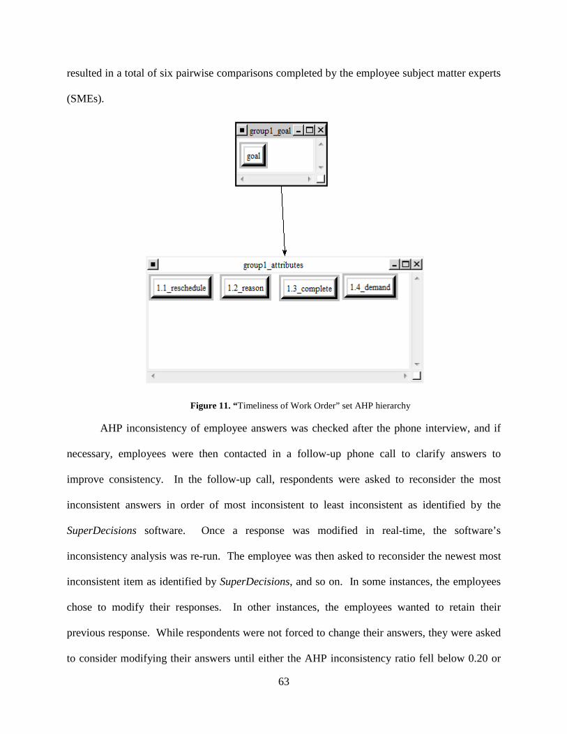
63
resulted in a total of six pairwise comparisons completed by the employee subject matter experts
(SMEs).
Figure 11. “Timeliness of Work Order” set AHP hierarchy
AHP inconsistency of employee answers was checked after the phone interview, and if
necessary, employees were then contacted in a follow-up phone call to clarify answers to
improve consistency. In the follow-up call, respondents were asked to reconsider the most
inconsistent answers in order of most inconsistent to least inconsistent as identified by the
SuperDecisions software. Once a response was modified in real-time, the software’s
inconsistency analysis was re-run. The employee was then asked to reconsider the newest most
inconsistent item as identified by SuperDecisions, and so on. In some instances, the employees
chose to modify their responses. In other instances, the employees wanted to retain their
previous response. While respondents were not forced to change their answers, they were asked
to consider modifying their answers until either the AHP inconsistency ratio fell below 0.20 or
64
until there were no more comparisons to modify. The AHP inconsistency ratio is a measure of
the inconsistency in a decision maker’s pairwise comparisons. For example, if item A is ranked
higher than item B and item B is ranked higher than item C, then item A should be ranked higher
than item C. This may not always happen or may not happen to the proper degree from the
Fundamental Scale when pairwise comparisons are being made. Thus, the ratio measures the
degree of inconsistency in the judgments. It was not always possible to improve the
inconsistency ratio below 0.20 because some employees just did not want to modify highly
inconsistent answers. Saaty recommends an inconsistency ratio of 0.10 or less for the AHP
(Saaty, 1980; 1990). However, because inconsistency is not error but rather variation in the data
and because the judgments are eventually combined, an inconsistency ratio greater than 0.10 at
the individual level does not degrade the overall results for a group of judgments. More
importantly, the inconsistency of the combined judgments will be less than the greatest
inconsistency of any individual judgment in that group (Vargas, 2010). Therefore, we aimed for
an inconsistency of 0.20 or lower to ensure reasonable results once the results were aggregated.
Furthermore, some influence sets contain seven or eight items, causing quite a few (21 or 28
respectively) pairwise comparisons. It can be rather difficult for a decision maker to keep all the
comparisons clear and consistent when making this many judgments, so relaxing the
inconsistency ratio to 0.20 or less is appropriate. All pairwise comparisons for all influence sets
are shown in Appendix B.2.
65
4.5 AN EXAMPLE OF EMPLOYEE RESPONSES
To illustrate the interview process, examples of two employee responses in the “Timeliness of
Work Order” set are outlined below.
The “Timeliness of Work Order” set is the first set of influences and is described in detail
in Chapter 3. There are four influences in this set. As an example, consider the responses of
Employee #15 (who has a job title of “Online Work Week Manager” in the work management
department at the test bed company). His judgments for each of the six pairwise comparisons
(details of which are in Appendix B.2) along with his synthesized AHP priorities and
corresponding inconsistency ratio are shown in Figure 12 and Figure 13. Figure 12 is from the
SuperDecisions software, and the selected boxes denote his responses. Because 9 was dropped
from the ratio scale for these comparisons, only the scale values 1, 3, 5, and 7 were selected in
the software, according to responses from the SMEs. For example, in the pairwise comparison
between influence 1.1 and influence 1.2 (row 1 of the figure), influence 1.2, “Reason for the
Work Order,” was selected to be weakly more important than influence 1.1, “When the Work
Order Can be Rescheduled,” by Employee #15, evident by a score of 3 using Saaty’s
Fundamental Scale. Figure 13 shows that, after AHP synthesis, influence 1.3 is most important
to Employee #15 (priority score 0.4713), followed by influence 1.2, influence 1.4, and influence
1.1, shown by the decreasing priority scores.
As another example, Employee #18 is an “Outage Scheduling Supervisor” at the test bed
company. He provided the judgments shown in Figure 14, with AHP priorities and
inconsistency ratio as shown in Figure 15. Figure 15 shows that influence 1.1 (with a priority
score of 0.3190) is most important to Employee #18 after the AHP synthesis.
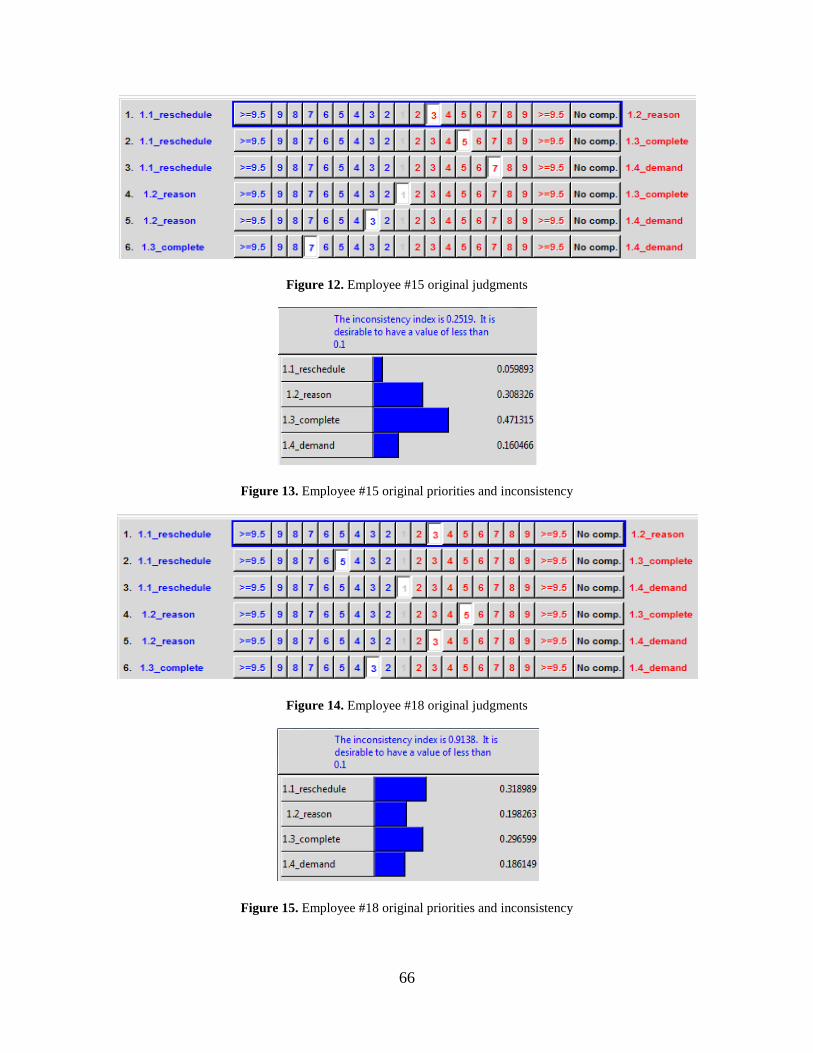
66
Figure 12. Employee #15 original judgments
Figure 13. Employee #15 original priorities and inconsistency
Figure 14. Employee #18 original judgments
Figure 15. Employee #18 original priorities and inconsistency
67
Note that the original inconsistency is high for both Employees #15 and #18, 0.2519 and
0.9138 respectively. Therefore, the employees were asked to revise their judgments in a follow-
up call, and the revised outcomes and priorities are shown in Figure 16, Figure 17, Figure 18,
and Figure 19. As shown in Figure 16, Employee #15 modified the sixth pairwise comparison
between influence 1.3 and influence 1.4, changing his original judgment of influence 1.3 as very
strongly more important than influence 1.4 (Figure 12) with a value of 7 to the two influences
being equally important as depicted with a value of 1 in Figure 16. This shifted his most
important influence to influence 1.2 after AHP prioritization (priority score of 0.3806), as shown
in Figure 17. Employee #18 revised his judgments for the fourth and fifth pairwise comparisons,
as shown in Figure 18. This modified his most important influence to influence 1.2 (priority
score of 0.5177), as shown in Figure 19. Clearly, the follow-up phone call process provided
improvement in Employee #15’s score, as his inconsistency ratio is now under 0.20, decreasing
from 0.2519 to 0.1330. Employee #18 changed some answers but not enough responses to lower
his inconsistency under 0.20. His original inconsistency ratio was 0.9138, and after the follow-
up call, it decreased to 0.2623. These are the best results we could obtain for the individual
respondents without forcing the participants to change answers. Taking this approach allows for
the most consistent answers while preventing the data from being skewed or interfered with by a
third party.
This process of interviewing individual SMEs and then following up with those whose
inconsistency ratios were greater than 0.20 continued with one iteration of follow up calls. Once
all scores were obtained, aggregating the scores was necessary, as the overall AHP process and
hierarchy requires a single set of judgments. Thus, the sets of responses from the five different
decision makers in the group comparing influences in the “Timeliness of Work Order” set must

68
be aggregated into one set of judgments. The following section describes the process of AHP
aggregation and subsequent data limitations.
Figure 16. Employee #15 revised judgments
Figure 17. Employee #15 revised priorities
Figure 18. Employee #18 revised judgments

69
Figure 19. Employee #18 revised priorities and inconsistency
4.6 GROUP AGGREGATION
The final revised judgments for the five decision makers in the “Timeliness of Work Order” set
are shown in matrix form in Table 6. Full revised judgments for all other sets are shown in
Appendix B.3. Employee #s 14, 16, and 17 are also included in this group. For each pairwise
comparison, employee judgments appear in numerical order: Employee #14, Employee #15,
Employee #16, Employee #17, Employee #18.
Table 6. Revised judgments for all respondents in the “Timeliness of Work Order” set
Judgments for Employees 14, 15, 16, 17, 18
vs. 1.1 1.2 1.3 1.4
Judgments
1.1 1 1/5, 1/3, 3, 1/7, 1/3 1/5, 1/5, 1/3, 1/5, 5 5, 1/7, 3, 1/3, 1
1.2 1 1/5, 1, 1/5, 1, 5 3, 3, 1/3, 5, 5
1.3 1 1/7, 1, 5, 5, 3
1.4 1

70
Normally the geometric mean of the five values in each box would simply be taken to
aggregate the judgments, but in accordance with recent work by Saaty and Vargas (2007), a
dispersion test was performed. All sets of comparisons in the “Timeliness of Work Order” set
failed the test, implying too much dispersion around the geometric mean. This dispersion
possibly may be attributed to the different functional areas and knowledge backgrounds of the
SMEs. Therefore, another method of group aggregation is needed to aggregate the appropriate
results for these data. In theory, it is recommended that one should return to the decision makers
in an attempt to have them revise judgments when the geometric mean cannot be accurately
used. However, when follow-up with respondents occurred, the employees did not always wish
to modify their judgments any further. Therefore, dispersion could not always be improved.
Due to the limitations and impracticality of the Basak (1988) and Basak and Saaty (1993)
method, another method is clearly needed to address AHP group aggregation when dispersion
around the geometric mean is violated and respondents are unwilling or unable to revise their
judgments. A new approach using principal components analysis (PCA) is developed in this
dissertation. While this method is critical for proper group aggregation, it is not directly relevant
to the overall ranking of influences, and a detailed description of the method is postponed to
Chapter 5. PCA is a statistical technique that transforms a set of (most likely correlated)
variables into a smaller set of uncorrelated variables (Dunteman, 1989).
The new PCA based AHP group aggregation method was used to aggregate the
judgments for all influence sets, including ranking the overall set of influences with the
exception of set seven. The five SMEs’ judgments in set seven (“Cost Consequences”) passed
the dispersion test, so the geometric mean was used to aggregate their judgments. The final
aggregated judgments for the “Timeliness of Work Order” set are shown in Table 7; the

71
aggregation develops one representative judgment across all employees who evaluated that set.
Appendix B.4 contains the aggregated judgments for all other sets of influences and the seven
overall sets of influences.
Table 7. Aggregated group judgments for the “Timeliness of Work Order” set
Influences vs. 1.1 1.2 1.3 1.4
Influences
1.1 1 0.6922 2.4942 1.1536 1.2 1 2.7524 4.0639 1.3 1 3.6037 1.4 1
The final AHP prioritization weights are shown in Table 8. Note that the numbers in
each column sum to 1.0 and the priority vectors for each influence set as well as for the overall
set of influences are derived (respectively) from Table 7 and Appendix B.4 using the traditional
AHP synthesis. For example, Table 8, column 1 shows the priorities found using the aggregated
group judgments for set 1 (Table 7). The first row of each column in Table 8 shows the priority
for the first influence in the set, the second row shows the priority for the second influence, and
so on. Therefore, for the “Timeless of Work Order” set, influence 1.2 is the most important
influence, as it has the column’s maximum priority of 0.4151. Column 0 represents the group of
overall influences that was ranked by the managers. Thus, the influences from the diagram in
Chapter 3 have been weighted through the AHP via group aggregation using PCA (sets 1-6 and
0) or the geometric mean (set 7). The next step is to use these weights in formulating criticality
scores for each spare part (Chapter 6).
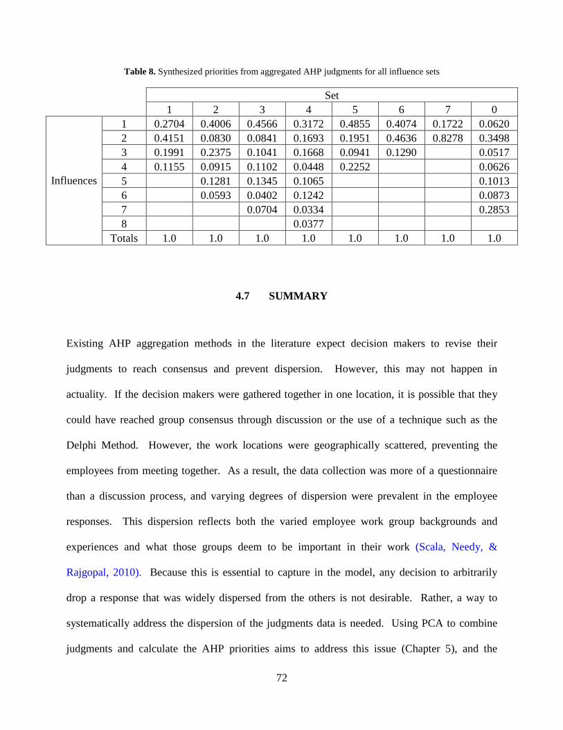
72
Table 8. Synthesized priorities from aggregated AHP judgments for all influence sets
Set 1 2 3 4 5 6 7 0
Influences
1 0.2704 0.4006 0.4566 0.3172 0.4855 0.4074 0.1722 0.0620 2 0.4151 0.0830 0.0841 0.1693 0.1951 0.4636 0.8278 0.3498 3 0.1991 0.2375 0.1041 0.1668 0.0941 0.1290 0.0517 4 0.1155 0.0915 0.1102 0.0448 0.2252 0.0626 5 0.1281 0.1345 0.1065 0.1013 6 0.0593 0.0402 0.1242 0.0873 7 0.0704 0.0334 0.2853 8 0.0377
Totals 1.0 1.0 1.0 1.0 1.0 1.0 1.0 1.0
4.7 SUMMARY
Existing AHP aggregation methods in the literature expect decision makers to revise their
judgments to reach consensus and prevent dispersion. However, this may not happen in
actuality. If the decision makers were gathered together in one location, it is possible that they
could have reached group consensus through discussion or the use of a technique such as the
Delphi Method. However, the work locations were geographically scattered, preventing the
employees from meeting together. As a result, the data collection was more of a questionnaire
than a discussion process, and varying degrees of dispersion were prevalent in the employee
responses. This dispersion reflects both the varied employee work group backgrounds and
experiences and what those groups deem to be important in their work (Scala, Needy, &
Rajgopal, 2010). Because this is essential to capture in the model, any decision to arbitrarily
drop a response that was widely dispersed from the others is not desirable. Rather, a way to
systematically address the dispersion of the judgments data is needed. Using PCA to combine
judgments and calculate the AHP priorities aims to address this issue (Chapter 5), and the

73
aggregated priorities become the weights for the influences in the part scoring model (Chapter
6). In this model, the actual test bed company spare parts data is combined with the influence
weights to formulate a criticality score for each spare part. The parts are then placed into one of
three groups (I, II, or III) based on their criticality score, with the groups reflecting the
importance of keeping the part in inventory with respect to the company bottom line. The
overall objective is to minimize plant downtime and subsequent revenue loss in a cost effective
manner.
The use of AHP and aggregation of group judgments allows for representation of the
range of knowledge and expectations across work groups and locations. The methodology
presented in this dissertation collects the experiences of multiple employees and synthesizes their
qualitative data into a set of priorities for the influences to the spare parts process. The varied
employee opinions can be brought together in a format that represents the overall goals and
needs of the company, while recording critical knowledge of employees, many of whom are on
the verge of retirement or attrition. The process of identifying influences and weighting them
through group aggregation of the AHP, whether or not dispersion around the mean exists, can be
applied in a multitude of corporate settings and to a varied set of decision making needs beyond
spare parts. Such studies will capture corporate knowledge as well as balance corporate culture
and decision making through continuous improvement and improved business practices.

74
5.0 PRINCIPAL COMPONENTS ANALYSIS (PCA) BASED METHOD FOR GROUP
AGGREGATION IN THE ANALYTIC HIERARCHY PROCESS (AHP)
Chapter 4 discussed the interview protocol for group judgment of the 34 influences to the spare
parts process. These group judgments (except set 7) failed Saaty and Vargas’ (2007) dispersion
test both before and after respondents were given a chance to revise their judgments. Limitations
in the literature regarding how to proceed with group aggregation in this situation were briefly
discussed in Chapter 4. This chapter extends the discussion of the current literature and presents
a new AHP group aggregation technique through the use of principal components analysis
(PCA). The method essentially uses a weighted geometric mean to aggregate the judgments,
with PCA used to determine the weights for each decision maker. Details of the method along
with illustrative examples are included in this chapter.
5.1 MOTIVATION FOR PCA BASED METHOD
The Analytic Hierarchy Process (AHP) is a structured approach for making decisions in a
complex environment. Often it is appropriate to have more than one decision maker perform the
pairwise comparisons in the AHP analysis. This allows for multiple points of view and multiple
subject matter expertise to play a role in the final decision. These multiple decision makers can
work independently, spread out over multiple geographic locations, or they could be in a

75
centralized setting. Their analysis leads to individual judgments which could then be aggregated
into group judgments in order to obtain a more robust set of comparisons. Traditionally, the
geometric mean has been used for this purpose because it has been shown by Aczél and Saaty
(1983) to be the only aggregation method that does not violate the properties of the AHP. In this
approach, for a given pairwise comparison, the geometric mean of the judgments across all of the
decision makers is computed and used as the aggregate judgment for the group. This is done for
all sets of pairwise comparisons in the AHP hierarchy. Furthermore, if each decision maker is
not to be given equal consideration in the aggregation, then the weighted geometric mean is used
to combine judgments (Aczél & Alsina, 1987). There are many case studies in the AHP
literature where the geometric mean was directly used to aggregate group judgments. Examples
include Armacost, Hosseini, and Pet-Edwards (1999) and Liberatore and Nydick (1997).
With group judgments we hope for broad consensus among the decision makers.
However, in practice this will not always be the case. The natural question then arises whether
it is appropriate to use the geometric mean to perform pairwise comparison aggregation in
conditions where a consensus cannot be reached and significant dispersion exists among the
judgments. Saaty and Vargas (2007) address this question and recently showed that the
geometric mean cannot automatically be used in all instances. Specifically, they recommend
first performing a statistical test for dispersion around the mean.
Basically, the test is designed to determine if the observed variance in the set of group
judgments for a given pairwise comparison is typical, given the group’s behavior. The authors
show that as the number of decision makers (m) increases, the geometric dispersion of the
comparisons tends to follow a gamma distribution whose shape and scale parameter values can
be determined for any value of m. Thus, their statistical test determines the probability (p) of

76
observing a geometric dispersion of the group judgments that is no larger than the calculated
(sample) value for the group. If this probability is sufficiently small, then it would indicate that
there is a high probability (1-p) of observing geometric dispersions that are at least as large as the
calculated value, implying that the observed dispersion is not unusually large and the geometric
mean can be used. Conversely, if the p-value is large, the judgments are deemed to fail the
dispersion test, and using the geometric mean to aggregate the judgments across that particular
pairwise comparison would be inappropriate. In practice, most sets of pairwise comparisons
must pass the dispersion test in order for the geometric mean to be used to aggregate all
judgments and sets of pairwise comparisons in the AHP hierarchy. Further discussion and
details on how to perform the dispersion test are given in Saaty and Vargas (2007).
Unfortunately, when dispersion across judgments is too large and the geometric mean
cannot be used, there appears to be no clear guidance in the literature on an alternate approach to
aggregate group judgments. The most relevant literature on this topic appears to be the work of
Basak (1988) and Basak and Saaty (1993), who look at a related problem. In their work the
decision makers are divided into separate groups. The authors take a statistical approach and
present a method where the groups are tested for homogeneity to see if some or all of the groups
can be combined. This method assumes a large number of geographically dispersed decision
makers and uses maximum likelihood estimators with the likelihood ratio test. It also assumes
that the judgments of the decision makers are distributed lognormally, which may or may not be
true for a given group of decision makers’ judgments. However, the authors do not address how
the decision makers are initially grouped together. More importantly, while their method
identifies when groups can be pooled and when they cannot, it does not provide guidelines on
what to do in the latter case.

77
Basak (1988), Basak and Saaty (1993), Aczél and Saaty (1983), Aczél and Alsina (1987),
and Saaty and Vargas (2007) all argue that the decision makers should be asked either to
reconsider and revise their judgments when consensus cannot be reached or to work together to
reach consensus. If the decision makers choose to revise their judgments, and the corresponding
set of pairwise comparisons is reasonably consistent (i.e., the inconsistency ratio is low), then
those revised judgments may be substituted for the decision maker’s original judgments in group
aggregation. Another dispersion test should be performed, and if the set of aggregated
judgments passes the test, then the geometric mean can be used to aggregate the judgments.
In practice though, this process might not be feasible from a logistical or geographical
standpoint. Moreover, the decision makers might not want to revise their judgments, or the
revised judgments might still not pass the dispersion test. Both situations were evident in the
group judgments on the influences in Chapter 4. Generally, these situations could also be quite
possible in survey situations, for example, where the decision makers are geographically
dispersed or responding without group interaction. The AHP literature has not addressed, to our
knowledge, the question of how one should proceed with group judgment aggregation when the
dispersion test fails and the decision makers are unwilling or unable to revise their judgments. A
suggested alternative in such situations is to use the weighted geometric mean; this preserves the
unanimity, homogeneity and the reciprocal property that are crucial to the AHP. It also serves
the role of assigning different weights to each judge in the group, as presumably the judges are
not all consistent to the same degree. However, to our knowledge there has been no research
aimed at determining exactly how the weights for computing the weighted geometric mean
should be selected.

78
In this chapter, we propose a new method for aggregating judgments when the raw
(unweighted) geometric mean cannot be used and the decision makers are unwilling or unable to
revise their judgments. Our method makes use of PCA to combine the judgments into one
aggregated value for each pairwise comparison. We show that this approach is equivalent to
using a weighted geometric mean with the weights coming from the PCA. The remaining
portion of the chapter provides a brief overview of PCA and describes how it can be applied to
group decision making with the AHP, including an illustrative example. Discussion regarding
both how this approach is equivalent to using a weighted geometric mean and why the approach
is appropriate is included. Finally, convergence of the priority vector from a weighted geometric
mean based on PCA to the priority vector obtained from the raw geometric mean is
demonstrated.
5.2 OVERVIEW OF PCA
PCA is a statistical technique that uses an orthogonal linear transformation to transform a set of
(most likely correlated) variables into a smaller set of uncorrelated variables (Dunteman, 1989).
In essence, PCA attempts to reduce the dimensionality of a data set by distilling it down to the
components that capture the majority of the variability associated with the original data set. In
our context, this is obviously appealing because we seek a way to capture most of the variability
among the judges. The procedure addresses the variance / covariance structure of the data and
uses the eigenvectors of the covariance matrix to transform the data to a new coordinate system
in which the original data is rotated on its axes such that maximum variance of any projection of
the data lies along the first coordinate (the first principal component), the second largest variance
79
along the second coordinate (the second principal component), and so on. Thus, if we start with
a set of n observations in m variables, PCA reduces the original data set to n observations on k
components that capture a large proportion of the total variance. Principal components are used
for data reduction and interpretation and are typically employed in large analyses, revealing
relationships in the data that might not originally be evident. The method has been widely
applied in practice, including areas such as biology, medicine, chemistry, and geology
(Dunteman, 1989). Further description of principal components can be found in Johnson and
Wichern (2007), Jolliffe (2002), and Dunteman (1989). However, to our knowledge, PCA has
not previously been used for group aggregation in the AHP.
5.3 PRINCIPAL COMPONENTS AND THE AHP
Consider group judgments in the context of the AHP. Each of the n pairwise comparisons made
by the set of decision makers may be viewed as analogous to an observation in PCA, and each of
the m decision makers may be viewed as a variable or as one dimension of the data set. The
decision makers themselves are different, and thus one would expect to see some variability in
the numerical scores assigned by them to a given pairwise comparison. However, the scores are
also likely to be correlated because each decision maker is judging the same paired comparison.
The objective of the principal components analysis would then be to determine the (uncorrelated)
principal components that capture the majority of the variability among the judges.
In practice, before PCA is applied, we transform the individual judgments into their
logarithms in order to reduce the problem to one of finding the best set of weights for use with a
weighted geometric mean (GM). Suppose decision maker k is assigned a weight 𝑤𝑘 where

80
𝑤𝑘 ∈ (0,1) and ∑ (𝑤𝑘) = 1. 𝑘=1…𝑚 Furthermore, let 𝑎𝑖𝑗𝑘 represent the value from Saaty’s
Fundamental Scale chosen by decision maker k in comparing factor i with factor j. Let us also
denote by aij the weighted geometric mean of these values across all of the judges, i.e., 𝑎𝑖𝑗 =
∏ (𝑎𝑖𝑗𝑘 )𝑤𝑘𝑚𝑘=1 . First note that if aij is used as the final synthesized value for the comparison
between factors i and j, then as desired in the AHP, 𝑎𝑗𝑖 = ∏ (1 𝑎𝑖𝑗𝑘⁄ )𝑤𝑘𝑚𝑘=1 = �1 𝑎𝑖𝑗⁄ �. Now
suppose that we replace 𝑎𝑖𝑗𝑘 with log(𝑎𝑖𝑗𝑘 ). Clearly if we compute the weighted arithmetic mean
we obtain ∑ 𝑤𝑘𝑙𝑜𝑔 (𝑎𝑖𝑗𝑘 )𝑚𝑘=1 = 𝑙𝑜𝑔 �∏ (𝑎𝑖𝑗𝑘 )𝑤𝑘𝑚
𝑘=1 � = 𝑙𝑜𝑔 (𝑎𝑖𝑗), and the corresponding value in
the transposed entry is equal to 𝑙𝑜𝑔 (1/𝑎𝑖𝑗). Exponentiating these values yields results that are
identical to those from the weighted GM.
We therefore first replace all of the original comparison values with their logarithms. We
then compute the principal components and restrict ourselves to the first principal component,
which is the eigenvector corresponding to the largest eigenvalue of the corresponding covariance
matrix. This m-vector captures the majority of the variance; we then normalize and use this to
develop final aggregated values for the numerical comparisons, which in turn are then used to
develop the final set of priorities in the AHP. Note that this does not involve any assumptions
about the distributions of the pairwise comparisons. This approach may also be viewed as a way
of obtaining a “correct” set of weights when developing the priority vector in the context of
group aggregation via the weighted geometric mean. Later in this chapter, we further examine
this approach by studying how the weights behave with respect to the magnitude of the
disagreement among the judges and show that as the dispersions tend to zero, the weights from
the PCA tend to equal values for all the judges, so that the weighted GM converges to the raw
GM. Thus, this PCA-based method for developing weights can be used with any data set where
Saaty and Vargas’ (2007) test for dispersion around the geometric mean is violated, the decision
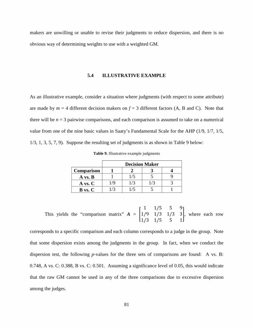
81
makers are unwilling or unable to revise their judgments to reduce dispersion, and there is no
obvious way of determining weights to use with a weighted GM.
5.4 ILLUSTRATIVE EXAMPLE
As an illustrative example, consider a situation where judgments (with respect to some attribute)
are made by m = 4 different decision makers on f = 3 different factors (A, B and C). Note that
there will be n = 3 pairwise comparisons, and each comparison is assumed to take on a numerical
value from one of the nine basic values in Saaty’s Fundamental Scale for the AHP (1/9, 1/7, 1/5,
1/3, 1, 3, 5, 7, 9). Suppose the resulting set of judgments is as shown in Table 9 below:
Table 9. Illustrative example judgments
Decision Maker
Comparison 1 2 3 4 A vs. B 1 1/5 5 9 A vs. C 1/9 1/3 1/3 3 B vs. C 1/3 1/5 5 1
This yields the “comparison matrix” A = �1 1/5 5 9
1/9 1/3 1/3 31/3 1/5 5 1
�, where each row
corresponds to a specific comparison and each column corresponds to a judge in the group. Note
that some dispersion exists among the judgments in the group. In fact, when we conduct the
dispersion test, the following p-values for the three sets of comparisons are found: A vs. B:
0.748, A vs. C: 0.388, B vs. C: 0.501. Assuming a significance level of 0.05, this would indicate
that the raw GM cannot be used in any of the three comparisons due to excessive dispersion
among the judges.

82
With the PCA approach, we start by defining the transformed matrix A’, where each entry
is the logarithm of the corresponding entry in A. Any standard package (e.g., MATLAB) can
verify that the first principal component (the unit eigenvector corresponding to the largest
eigenvalue of the covariance matrix for A’) is the vector [0.5596 0.1513 0.8022 0.1430]T. Note
that this vector has its l-2 (Euclidean) norm equal to 1. Because the AHP approach uses the l-1
norm, we simply square each element (so that they sum to 1.0) to obtain w = [0.3132 0.0229
0.6434 0.0205]T. Vector w could be viewed as a vector of final “weights” to be given to each
judge, with the aggregated value for each comparison given by z’ = A’w = [1.0437 -1.3977
0.6546]T. In order to arrive at the original scale, we now reverse the transformation by
exponentiating each element of z’ to obtain z = [2.8397 0.2472 1.9244]. Thus the symmetric
matrix SP for computing the AHP priorities is shown with row and column labels as Table 10.
Table 10. Symmetric matrix SP for computing the AHP priorities
A B C A 1 2.8397 0.2472 B 1/2.8397 1 1.9244 C 1/0.2472 1/1.9244 1
The normalized principal right eigenvector for this matrix yields the final priority vector for the
AHP, namely vP = [0.2915 0.2882 0.4203]T.
Note that if instead we had used the geometric mean of the four values, one from each
decision maker for each pairwise comparison (row in matrix A), we obtain the vector z = [1.7321
0.4387 0.7598]T and the following symmetric matrix SG for computing priorities, shown as
Table 11 with row and column labels. The principal eigenvector for this matrix yields the
priority vector vG = [0.2930 0.2439 0.4631]T. In the absence of an alternative approach, vG
would be used.

83
Table 11. Symmetric matrix SG for computing the AHP priorities
A B C A 1 1.7321 0.4387 B 1/1.7321 1 0.7598 C 1/0.4387 1/0.7598 1
The less dispersion among the judges, the closer these two different vectors are to each
other. For instance, suppose the original comparison matrix was A = �3 3 5 5
1/7 1/7 1/9 1/71/9 1/7 1/7 1/7
�;
in this case, less dispersion exists among the judges as compared to the previous example. It can
be shown that the two priority vectors are given by vP = [0.1637 0.0651 0.7712]T for the PCA
based approach and vG = [0.1626 0.0659 0.7715]T for the approach based on the raw GM. Note
these are very similar to each other. In particular, consider the limiting case when no dispersion
exists and the decision makers are perfectly consistent in their judgments. In this instance each
n-dimensional column vector in A is identical to all judges assigning exactly the same scores to
any comparison. In this situation the first principal component is a vector w of dimension m,
with each entry equal to 1/m; i.e., each of the m judges is assigned the same weight of 1/m. Thus
the weighted GM is identical to the raw GM, and the final priority vectors vP and vG are identical.
5.5 CONVERGENCE OF VP TO VG
As shown in the previous section, the vectors vP and vG are identical when no dispersion exists
among the judges. However, when there is significant dispersion, we would expect these two
vectors to be quite dissimilar. In this section we describe an empirical study with two objectives:
(1) to understand the limiting behavior of the PCA based approach as diversity of opinion among

84
the decision makers decreases, and (2) to see if the PCA based approach converges uniformly to
results from the GM based approach. The data for the study are generated from a simulation
model. Before describing the range of parameter values studied, we first describe how “diversity
of opinion” (i.e., dispersion) is captured by the study. For any pairwise comparison, the
numerical value assigned can take on one of the nine values on Saaty’s Fundamental Scale.
Moreover, the scale is monotonic in the sense of strength of preference for one alternative over
the other, so that a value of 1/9 would represent one end of the opinion spectrum and a value of 9
the other end. Thus if the decision makers are consistent, they would assign values for the
comparison that are close to each other, while a divergence of opinion would result in values that
cover a wider range. Now, suppose we number each of the nine values on the scale as a “unit” as
shown in Table 12 below:
Table 12. Saaty’s Fundamental Scale values assigned to units
Unit Value 1 1/9 2 1/7 3 1/5 4 1/3 5 1 6 3 7 5 8 7 9 9
To capture variation among the decision makers, we then define the “scale spread” (δ) as
the range of units covered by the values assigned by different decision makers in the group. So,
for example, if δ = 2 all decision makers choose one of two consecutive units on the scale, such
as 1/9 and 1/7, or 1 and 3, or 5 and 7. On the other hand, if δ = 5 they all choose values from a
set of 5 consecutive units on the scale (e.g., {1/7, 1/5, 1/3, 1, 3} or {1/3, 1, 3, 5, 7} or {1, 3, 5, 7,

85
9}). We ensure that at least one judge picks the smallest value and another the largest value in
the range so that the actual diversity of opinion is captured. In the two extreme cases, if δ = 1,
then all decision makers are perfectly consistent and choose the same value, while if δ = 9, their
values range across the entire spectrum of possible values (from 1/9 through 9). The two
extreme values in the scale spread are always selected for two of the judgments. The values for
the remaning judgments are randomly selected, with every value in the scale spread, including
the extremes, having an equal probability (1𝛿� ) of being selected. In order to conduct our study,
we vary three different parameters as follows:
a. The number of decision makers: m = 4, 5, 6, 7, 8, 10, 15, 25, 50
b. The number of factors or alternatives being compared with each other: f = 3, 4, 5, 6,
7, 8
c. The scale spread δ = 2, 3, 4, 5, 6, 7, 8, 9
Note that if f alternatives are being compared with each other, the actual number of
pairwise comparisons being made is 𝑛 = 𝑓(𝑓 − 1)/2; this would also be the number of rows in
the comparison matrix A. The objective is to study the difference between the priority vectors
from a PCA-based weighted GM approach and the traditional GM-based approach on the same
set of judgments when different levels of disagreement exist among the decision makers (as
measured by δ), across different values of m and f. Of course, if δ = 1 the priority vectors are
always identical.
For a given combination of values for m, f and δ, we randomly generated a set of m
judgment values from the basic scale for each of the 𝑛 = 𝑓(𝑓 − 1)/2 pairwise comparisons,
while ensuring that these values always range over δ adjacent units on the scale, with both

86
extremes in the range definitely being selected. The specific units spanned for each individual
comparison could be different (e.g., with δ = 3, for A vs. B these might come from {3, 5, 7}
while for C vs. D the values might come from {1/3, 1, 3}). The corresponding priority vectors
using the PCA approach (vP) and the GM approach (vG) are then computed along the lines of the
example in Section 5.4. A full factorial experiment yields a total of |𝑚| ∗ |𝑓| ∗ |𝛿| = 9 ∗ 6 ∗ 8 =
432 unique combinations, and for each combination, we ran 10,000 simulations and computed
the mean and standard deviation of the distances across these replications. Note that in each
replicate there are n separate pairwise comparisons.
Before comparing vectors vP and vG, we first examine the circumstances under which a
GM based approach for aggregating group judgments might be inappropriate. To see this, for
each combination of inputs (m, f and δ), we also computed the percentage of the (10,000 ∗
𝑛) comparisons in the simulation where the GM-based approach would fail the Saaty and Vargas
(2007) dispersion test at a p value of 0.05; suppose we denote this percentage by 𝑎𝑚𝑓𝛿. First,
note that once the m and δ are fixed, f only determines how many comparisons are being made;
the individual comparisons are similar in that they have the same spread across the same number
of judges. Thus, we average the percentages across all values of f for a given combination of m
and δ; i.e., we compute α𝑚𝛿 = {∑𝑓=3,…,8α𝑚𝑓δ} / 6. Based on this, Table 13 depicts for each m,
the probability (𝑎𝑚𝛿)/100 that the dispersion test fails under a scale spread of δ. Combinations
that yield a value of 0.05 or lower are shaded. Figure 20 plots the results; each line represents a
given value of m. The results indicate that as the number of decision makers increases, the test
tolerates more divergence of opinion amongst the decision makers. When m is very large (25 or
50), a scale spread of 4 or 5 units seems tolerable; with very few judges (m = 4 or 5), even a
87
small spread of 3 units might be unacceptable. In general, these results imply the levels of
disagreement that would invalidate the use of the GM with different numbers of decision makers.
Table 13. Probability (𝒂𝒎𝜹)/100 that the dispersion test fails under a scale spread of δ
δ Number of Judges (m)
4 5 6 7 8 10 15 25 50 1 0.000 0.000 0.000 0.000 0.000 0.000 0.000 0.000 0.000 2 0.133 0.004 0.000 0.000 0.000 0.000 0.000 0.000 0.000 3 0.421 0.327 0.217 0.125 0.102 0.06 0.008 0.001 0.000 4 0.758 0.584 0.497 0.407 0.359 0.252 0.139 0.033 0.008 5 1.000 0.937 0.818 0.747 0.672 0.546 0.405 0.241 0.072 6 1.000 1.000 0.977 0.936 0.927 0.874 0.761 0.589 0.395 7 1.000 1.000 0.997 0.98 0.974 0.964 0.94 0.905 0.838 8 1.000 1.000 1.000 0.993 0.987 0.986 0.985 0.986 0.991 9 1.000 1.000 1.000 0.997 0.993 0.992 0.995 0.998 1.000
Figure 20. Probability (𝒂𝒎𝜹)/100 that the dispersion test fails under a scale spread of δ
In comparing the vectors vP and vG, it is natural to use some sort of a distance measure.
However, note that the priority vectors do not have the same dimension—they belong to 𝑅+𝑓 (and
have an l-1 norm equal to 1). Therefore a distance measure (d) between the two vectors should
account for the value of f. We use the following adjusted version of the l-∞ norm: 𝑑 =
0.0000.1000.2000.3000.4000.5000.6000.7000.8000.9001.000
1 2 3 4 5 6 7 8 9
Pr(d
ispe
rsio
n te
st fa
ils; p
=0.0
5)
Scale Spread (δ)
m=4m=5m=6m=7m=8m=10m=15m=25m=50
m = 4
m = 50

88
�𝑀𝑎𝑥𝑖=1,…,𝑓�𝑣𝑖𝑃−𝑣𝑖
𝐺��(1 𝑓⁄ )
∗ 100. The denominator represents the average priority value for a set of f
factors, so that d represents the distance constituted by the l-∞ norm as a percentage of this
average.
Figure 21 displays a series of plots, one for each value of f. In each graph we plot the
distance d as a function of δ for each of the nine values of m. To maintain visual consistency, all
plots have the same scale. As δ approaches 1 (i.e., consistency among the judges is approached),
the distance d converges uniformly to zero in all cases. Figure 21 also yields other interesting
observations. First, for any fixed value of f and δ, the distance between vG and vP is always
smaller when the number of judges is larger. This is intuitive; for the same level of dispersion,
the effect of one individual judge is less pronounced if more judges are participating in the
pairwise comparisons. Second, for any fixed f, differences between vG and vP generally do not
seem to depend strongly on the number of judges when there is relatively little dispersion (say,
δ = 4 or lower) while the difference between the priority vectors as a function of m becomes
more pronounced when the dispersion is relatively large (say, δ = 6 or higher). Finally, while
distance between the priority vectors rises monotonically with dispersion in most cases, with a
very large number of judges (say 15 or more), the distance reaches a peak at δ = 6 or δ = 7 and
then starts to decrease with larger dispersion. However, in all cases, the graphs confirm that vG
and vP converge when dispersion is low or nonexistent. Thus, PCA is a viable technique to use
to develop decision maker weights. PCA captures the maximum variability amongst the decision
makers, accounting for the dispersion present in the data while combining the judgments so that
the dispersion test is not violated.

89
Figure 21. Distance d as a function of δ for values of f
0
5
10
15
20
25
30
35
40
45
50
1 3 5 7 9
dist
ance
(d)
dispersion (δ)
f=3m=4m=5m=6m=7m=8m=10m=15m=25
0
5
10
15
20
25
30
35
40
45
50
1 3 5 7 9
dist
ance
Id)
dispersion (δ)
f=4
0
5
10
15
20
25
30
35
40
45
50
1 3 5 7 9
dist
ance
(d)
dispersion (δ)
f=5
0
5
10
15
20
25
30
35
40
45
50
1 3 5 7 9
dist
ance
(d)
dispersion (δ)
f=6
0
5
10
15
20
25
30
35
40
45
50
1 3 5 7 9
dist
ance
(d)
dispersion (δ)
f=7
0
5
10
15
20
25
30
35
40
45
50
1 3 5 7 9
dist
ance
(d)
dispersion (δ)
f=8
m = 4
m = 25

90
5.6 SUMMARY
The method described in this chapter allows for aggregation of group judgments in the AHP
when the Saaty and Vargas (2007) dispersion test fails and respondents are unable or unwilling
to revise their judgments. The development of steps to aggregate judgments in this situation are
crucial to this dissertation; the dispersion test still clearly failed after experts at the test bed
company had the opportunity to revise their judgments. The complexity of and dispersion in the
experts’ responses are important to collect and maintain because this research develops a spare
parts inventory management methodology that encompasses all factors and forces relevant to the
spare parts process. Employee judgments and the relative importance of influences must be
accurately collected and aggregated to support accurate model development.
The lack of direction in the literature regarding what to do when the dispersion test fails
and decision makers are unwilling or unable to revise their judgments clearly indicates a need for
the PCA-based group aggregation method developed in this chapter. The AHP group
aggregation literature did not formally consider dispersion around the geometric mean until the
Saaty and Vargas (2007) dispersion test. It is quite possible that previous studies in group
aggregation used the raw geometric mean inappropriately (without knowing so). The benefits of
this PCA-based approach is that the weighted geometric mean can still be appropriately used to
aggregate AHP group judgments with the PCA being used to determine an appropriate weight
for every decision maker. The current literature does not discuss methods to analytically
determine weights for decision makers without subjectivity. Thus, this PCA-based approach also
contributes a systematic procedure for determining decision makers’ weights, regardless of
whether significant dispersion around the geometric mean does or does not exist.

91
Section 4.6 of Chapter 4 and Appendix B.4 present the final aggregated group judgments
and AHP priority weights for all sets of influences using the PCA-based method developed in
this chapter. The next chapter employs these weights as part of the criticality part scoring
technique and resulting classification of parts into inventory management groups.

92
6.0 PART CRITICALITY SCORES AND CLASSIFICATION
The next step in determining the importance of keeping a part in inventory is to develop a
criticality score for each part. Parts can then be grouped based on the corresponding scores. The
score combines the influence weights with actual data / relevant part information and assigns a
score along an ordinal scale. This chapter addresses these steps and includes a literature review
on part grouping and classification techniques, a discussion on the sample of parts used for
analysis, a definition of and examples of ordinal part data, a definition of the model used to
evaluate the part scores, and an example of its use.
6.1 LITERATURE REVIEW
In this research, the nodes on the influence diagram were evaluated through the Analytic
Hierarchy Process (AHP) to form a weight for each influence (Chapter 4). All the influences
will be used in determining a criticality score for a part. The technique of using multiple criteria
in evaluating an inventory classification is called MCIC (multi-criteria inventory classification);
similar studies have been presented in the literature, including some studies employing the use of
the AHP. However, these studies are limited in scope or consider traditional inventory that has
regular turns. This research aims to address the limitations of the literature and develop
criticality evaluations for spare parts inventory.
93
ABC part classification can be done via a multitude of characteristics, but annual dollar
volume is most common (Zimmerman, 1975). The main motivation for the MCIC literature
using the AHP is that annual dollar volume alone is not always enough to classify parts
(Zimmerman, 1975; Ng, 2007; Flores, Olson, & Dorai, 1992). Papers in this research area argue
that many criteria are relevant in inventory classification, and / or using dollar volume alone to
classify parts may be limiting and misleading (Flores, Olson, & Dorai, 1992; Flores & Whybark,
1987; Partovi & Burton, 1993; Ramanathan, 2006). In particular, Flores, Olson, and Dorai
(1992) argue that relative importance and number of criteria used in classification may vary by
firm, and the use of the AHP will enable incorporation of multiple criteria. These authors use
four criteria—average unit cost, annual dollar usage, criticality, and lead time—in the AHP part
classification hierarchy and give sample pairwise comparisons for the criteria. These criteria are
consistently used in the MCIC literature when using the AHP. The criteria are then combined
with transformed part data to form a criticality factor for each part. The part data used is
mathematically transformed to a 0-1 scale.
Gajpal, Ganesh, and Rajendran (1994) also use the AHP to determine part criticality for
placing parts into three groups—Vital, Essential, and Desirable (VED). The authors argue that
use of the AHP is systematic and not subjective and that they present the first use of AHP in
spare parts criticality inventory management. Their AHP hierarchy is based on three criteria—
availability of production facility when part fails, type of spares required, and lead time—and
includes alternatives for each criteria. Composite weights are found by combining priorities
from the AHP synthesis; parts are assigned to a VED group based on the sum of the composite
weights as well as calculated cutoffs for each group. However, the use of only three criteria in
the AHP model is limiting and restrictive.

94
The four criteria from Flores, Olson, and Dorai’s (1992) hierarchy are also used in
Partovi and Burton (1993). Their approach to the AHP classification of parts uses the ratings
mode of the AHP for pairwise comparisons as each stock keeping unit (SKU) being classified is
considered an alternative in the model. AHP priorities of the four criteria are also combined with
characteristic values for part data. However, these characteristics values are qualitative;
examples include very high, average, short, low, etc. Decimal values on a 0-1 scale are assigned
to each qualitative part characteristic. Parts are placed into groups using a traditional ABC
assignment—15% in group A, 35% in group B, and 50% in group C. Braglia, Grassi, and
Montanari (2004) extend the AHP classification method and present a multi-attribute spare tree
analysis specifically for spare parts classification. The tree has four criticality classes combined
with strategies for managing parts in each group. The AHP is used to evaluate the decision at
each node in the tree. Although specially designed for spare parts, the model is complicated and
appears to be difficult to execute in practice.
Other MCIC inventory classification methods are reviewed in Rezaei and Dowlatshahi
(2010) and Huiskonen (2001). In particular, Huiskonen (2001) notes that spare parts
management research is split into veins of mathematical models and ABC based analyses.
Rezaei and Dowlatshahi (2010) present other methods to use besides the AHP for classification
and present their own model which is based on fuzzy logic. For comparison, a classification of a
sample set of parts is done with both their fuzzy model and an AHP analysis. The fuzzy model is
based on four critieria—unit price, annual demand, lead time, and durability—which is also
limiting and not comprehensive of the all relevant factors to the spare parts process.
Flores and Whybark (1987) use a matrix approach with MCIC to classify parts based on
two criteria. Although their work was novel and opened a new area of research, the model
95
becomes complicated and cannot be easily extended to more than two criteria. This is
considered to be a serious limitation by both Ng (2007) and Flores, Olson, and Whybark (1992).
Partovi and Burton (1993) note that Flores and Whybark’s (1987) matrix approach also assumed
that the weights of the two criteria must be equal. Nonetheless, the model combines dollar usage
with part criticality, as subjectively defined by managers, and argued that the costs of both
holding parts and the implications of not having parts are important in a classification model.
Cluster analysis and weighted linear optimization have also been used to classify parts.
The cluster analysis models, Cohen and Ernst (1998) and Ernst and Cohen (1990), compare costs
of management policies defined for a cluster of parts to costs of management policies defined for
each individual part. The cost tradeoffs in clustering the parts are a penalty for placing parts in
groups and loss of discrimination. Their case study is the auto industry. However, Rezaei and
Dowlatshahi (2010) argue that this model needs a lot of data to run and can be impractical in
practice; furthermore, the model must be rerun when new parts are added, causing a potential
change in parts’ classifications. The weighted linear optimization models use optimization to
solve for each criterion’s weight or part’s score, and multiple criteria are considered. The part
score presented in Ramanathan (2006) is found through a weighted additive function,
considering the four criteria commonly used in the literature. This model must be resolved for
each part, yielding a score for each part, one at a time. Although this can be time consuming, the
author suggests the model is simple for managers to understand. In fact, Huiskonen (2001)
argues that managers do not feel comfortable if they do not understand the basics of individual
models. Ng (2007) employs a weighted linear optimization model, where the decision maker
ranks importance of criteria only; no relative importance such as a pairwise comparison is made,
only a ranking. Weights on a scale of 0-1 are generated in the linear optimization, parts are

96
scored, and the ABC / Pareto Principle is used to place parts in groups. The author concedes that
the model can be limited by many criteria, as ranking by the decision makers becomes difficult.
Hadi-Vencheh (2010) extends the model presented in Ng (2007) by using a nonlinear
programming model, with the four criteria repeatedly used in the literature.
Overall, criticality is important in spare parts logistics (Huiskonen, 2001) and is
considered in many classification models. Huiskonen (2001) defines process criticality as
consequences caused by a failure of a part with a spare not readily available and identifies it as a
strong factor. However, the assessment of criticality can be subjective, as downtime costs can be
hard to quantify.
This dissertation addresses criticality of spare parts through the part scoring system
presented in this chapter and extends and improves the current literature in MCIC inventory
classification. Furthermore, the criticality determination is more comprehensive than those
presented in the current literature. This model considers all 34 influences from the influence
diagram (Chapter 3) and is not limited to the four criteria commonly used in the literature. Many
criteria are easily considered in this model without it becoming unmanageable. No issues exist
with ranking the influences, as experts from multiple areas are employed to rank the influence set
of which they have knowledge. This model is fully representative of the spare parts process
without limitation. The method developed in this dissertation can be applied anywhere and is not
specific to one industry or company; in contrast, the Flores and Whybark (1987) model was
unique to the case study presented. As we will see in this chapter, the classification groups are
not limited to three, as with traditional ABC analysis, but rather a number appropriate for the
data and parts being considered.
97
6.2 SELECTION OF SAMPLE DATA
In order to test and validate the part scoring model, a random sample of 200 active spare parts
was obtained from the test bed company. The sample was split into 100 parts designated
“engineering critical” and 100 parts designated “engineering non-critical.” “Engineering
critical” is a label given to parts whose failure may compromise plant operations or whose proper
functioning is considered critical to plant safety and operations. Parts that are classified as such
receive routine preventive maintenance (PM) to prevent failure. “Engineering non-critical” parts
may not compromise the plant in the event of a failure and do not receive routine PM. A third
class of parts, “engineering run-to-failure,” are also installed at a nuclear plant but are not
included in this study. These parts do not receive PM, and no urgent need exists to replace these
parts upon failure.
The test bed company supplied a list of all spare parts, both active and inactive, from one
nuclear plant in its fleet. This list contained 17,917 engineering critical parts and 10,832
engineering non-critical parts. Most parts on this list were inactive or obsolete, so the goal was
to find a random sample of active parts, or parts that had recent usage by the plant. The
implementation of SAP by the test bed company in June 2003 was determined to be a logical
starting point for the random sample time window. For the engineering critical parts, a part was
selected at random from the list, and the SAP data was searched to find positive plant demand
between June 2003 and August 2009. (The August 2009 endpoint was the time horizon cutoff
point determined by the test bed company.) If positive plant demands (demands less returns > 0)
existed in this window, the part was added to the random sample. If not, it was discarded, and
another part was chosen at random. This process continued until 100 engineering critical parts
were found and was then repeated for the engineering non-critical parts. In total, 278 critical

98
parts and 208 non-critical parts were examined in order to find 100 active parts for each
designation with positive demand usages during the time window. Two hundred parts was
considered a reasonable sample size as it provides enough part data to verify the model without
being too cumbersome while accurately representing various part demand patterns.
The test bed company provided historical data for the list of 200 random parts. This
actual part data was loaded into a Microsoft Access database and used in model verification and
analysis.
6.3 ORDINAL PART DATA
This section describes the development of a common scale for measuring the relative importance
of a part with respect to each influence; the parts are diverse and criticality can be measured
along different dimensions or in different units. This case arises in the data provided by the test
bed company for the random sample of parts that was selected for analysis. This measure of
importance is then used as an input to the scoring model. Note that this research develops a
scoring model for inventory criticality and by no means attempts to modify or supersede the
engineering criticality definitions for plant operation. This model strictly considers the
importance of keeping a part on hand in inventory at the plant.
Actual data from the test bed company for each part with respect to each influence on the
influence diagram is used for creating the inputs to the scoring model. The word “data” is used
in a very general sense to encompass information relevant to the part. This data is diverse in
nature, with different characteristics that could be measured in different units (e.g., dollars, time,
counts, company codes, indicators, etc.) when the part is evaluated with respect to the various

99
influences. For example, cost consequences from lost revenues as a result of shutting a plant
down because a replacement part is unavailable after an emergent failure could run in the order
of millions of dollars in a deregulated market, while other influences, such as where the part is
installed inside the plant, are indicator variables (yes/no or 1/0 to indicate if a part is installed at a
given plant location).
To bring this part data to a common set of units for each influence, an ordinal scale of 1-5
is adopted for use as a basis for comparison and for distilling the different features of the data
across influences. This ensures that all influences are similarly represented and data from one
influence does not dominate that from others. The ordinal scale provides a base scale that is
unitless, allowing for equal representation of each influence, so that the weights from the AHP
prioritization (Chapter 4) can clearly differentiate the critical parts for inventory management.
Thus, the data, or part characteristics, can be easily compared by using a common reference scale
for all part data, which are values associated with the characteristics of the parts.
The scale developed herein assigns specific values or ranges of values for the data to
values 1-5 on the scale. This assignment is done for each influence uniquely. The scale value of
1 is reserved for the least critical values. Part data or data ranges assigned to the value 1 are
considered of little importance for keeping a part in inventory. This importance or criticality
increases with each scale value, with a value of 5 indicating highest importance. The
assignments of part data ranges to the ordinal scale are not necessarily linear. Moreover, the
assignment of data values to the scale is not necessarily straightforward in all cases due to the
diversity of the data in terms of both types and units. The process necessarily involves some
degree of subjectivity. When this is the case, assistance for appropriate scaling could come from
both subject matter experts (SMEs) and those who work with the part in question on a regular

100
basis. In general, the assignment of part data to the ordinal 1-5 scale would be easier when part
data is homogeneous, but this is not always the case. In particular, the part data supplied by the
test bed company is heterogeneous in units.
Some examples of part data include lists of purchase orders, reorder points, lists of
maintenance requests, and safety information. We use the actual historical part data, or values
found in the company’s Enterprise Resource Planning (ERP) system, in order to evaluate each
part and its importance to inventory. An ERP system is an information system used to plan
enterprise-wide resources needed to support customer orders (Heizer & Render, 2011). For the
test bed company, data on all part characteristics are stored in SAP, its ERP system. Numerous
characteristics are tracked and updated as time progresses and new data is available. In general,
some examples of data or characteristics that are typically stored in the ERP system include
vendor information, work orders, lead times, purchase orders, and bills of material (Heizer &
Render, 2011). In particular, for nuclear generation, data corresponding to plant refueling
outages and safety are also stored and tracked for every spare part. Data for all spare parts are
stored in the ERP system, including routine office supplies and parts that are obsolete or retired.
The ERP system provides the best and most comprehensive source for part data, and this
information is used to test and validate the scoring model. Uncertainty regarding important parts
is reduced because the data corresponding to these part characteristics capture the current
conditions of the parts and utilizes the limited amount of reliable and accurate data available.
To illustrate how the assignment might be done, two examples are given in the following
two subsections. In general, the item or part characteristic data for every influence will be
unique. These examples provide an illustration of what that data might be and how it could be
approached when applying this model to other industries.

101
6.3.1 Influence 2.1: Failure of Part Leads to LCO or SPV
This influence is the first influence in the “Part Failure” set, and the characteristic data counts the
number of LCO and SPV locations where a part is installed in a plant. Recall that a part failure
at an LCO location requires a full shut down of the plant unless the situation is fixed within a
relatively short interval of time following the failure (typically 72 hours). Therefore, the more
LCO locations at which a part is installed, the more critical it becomes, because there is an
increased probability that a failure of the part may shut down or force a derate of the plant. This
probability is based purely on the fact that as the number of LCO locations rises, a failure could
happen at more places. This influence does not consider the exact probability of such a failure
(because that data does not exist), but does indicate that such a failure could possibly occur.
A nuclear plant typically has two separate production lines that are identical and
redundant called “trains.” Generation of electricity can be done with either train, and the plant
switches between trains as maintenance is required or if a component failure occurs. Some parts
are installed common to both trains and are shared by both lines. Thus, a failure of one of these
parts can affect the production of electricity and may cause a derate or loss of production.
Locations where these parts are installed are called Single Point Vulnerability (SPV) locations.
To translate this characteristic to the ordinal scale, a list of the LCO and SPV locations at
where each part in the sample was installed was extracted from the test bed company ERP
system. Thus, 200 lists were extracted and the number of locations in each list was counted.
Reviewing these counts indicated that all 200 sample parts were installed at 24 or fewer LCO
and / or SPV locations. Therefore, 24 became the upper bound of the part data range, with 0 or
no LCO / SPV locations as the lower bound. The range of 0 to 24 must then be translated to the
dimensionless ordinal scale. Twenty-four was not simply divided by 5, which would assign an

102
equal number of possible counts to each bin (1-5) on the ordinal scale. Rather, the implications
associated with various counts of LCO / SPV locations and possible resulting complications
were considered. Zero was assigned to ordinal value 1 only because no LCO or SPV
installations imply no chance for plant shutdown and no effect on part criticality. Any LCO or
SPV installation count greater than 1 implies a non-zero probability of failure and shutdown,
which may result in millions of dollars of lost generation revenue. This revenue loss would
occur if a part was not in stock to remedy the situation quickly and / or the plant maintenance
team could not fix the issue in 72 hours or less.
Upon reviewing the counts of LCO and SPV locations in the random sample of 200 spare
parts at the test bed company, few parts were found to have greater than 7 LCO and / or SPV
installations, so the range corresponding to scale values 4 and 5 was widened. Doing so allows
for the parts with the most LCO / SPV installations to be considered most critical to inventory,
because these parts would be associated with ordinal scale values 4 and 5. Recall that a scale
value of 5 implies highest criticality and a scale value of 1 implies lowest or no criticality. In
summary, if the scale was not widened for counts greater than 7 and did not isolate 0 to a scale
value of 1, then an equal number of counts would be assigned to each scale value and the
complexity and nuances of corresponding inventory criticality associated with counts of LCO or
SPV locations would be lost. Table 14, row 2.1, shows the final scale assignments for influence
number 2.1.
6.3.2 Influence 1.3: Immediacy of Schedule—When to Complete the Work Order
This influence is the third influence in the “Timeliness of Work Order” set and addresses the
maintenance-related reason for a work order associated with a part. Every work order for

103
maintenance work is assigned a priority code that identifies how quickly the work needs to be
completed. Priority 100 or 200 codes are reserved for work that is likely to have immediate or
imminent impact on plant safety or generation output. These codes are reserved for the most
critical work and are rarely used. The priority 300 code is reserved for work that is emergent and
expedited, a failure in the plant that requires immediate attention. The priority 400 code
indicates time dependent work that must be done within 90 days. Priority 500, 600, 700, 800
codes are reserved for routine work or work that can be delayed indefinitely.
All historical work orders associated with all 200 parts in the random sample were
provided by the test bed company. Then the highest priority code for every part was identified in
the data. These priority codes were then matched with the corresponding part characteristic
value from the ordinal scale that matched the priority codes. The most critical work orders are
clearly priority codes 100 and 200, and priority code 300 and greater are associated with
corrective or routine work that cannot immediately shut the plant down. As such, the priority
codes were assigned to the ordinal scale values in the following manner: Priority 100 and 200 to
ordinal scale value 5, Priority 300 to ordinal scale value 3, priority 400 to ordinal scale value 2,
and priority 500, 600, 700, and 800 to ordinal scale value 1. As a result, priority codes were not
assigned the value of 4 from the ordinal scale.
6.4 SCALE ASSIGNMENTS
Ordinal scale assignments along the lines of the examples describe above were done for all 34
influences. Table 14 shows, for the nuclear spare parts data, the final mapping of the part data to
the ordinal scale along with the corresponding part characteristic data from the ERP system used
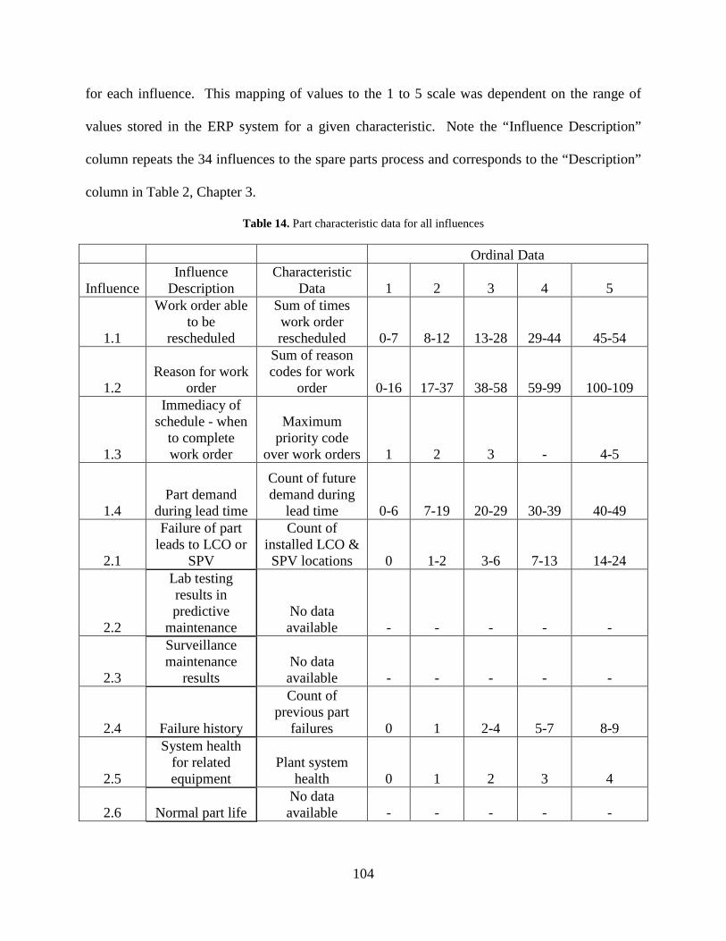
104
for each influence. This mapping of values to the 1 to 5 scale was dependent on the range of
values stored in the ERP system for a given characteristic. Note the “Influence Description”
column repeats the 34 influences to the spare parts process and corresponds to the “Description”
column in Table 2, Chapter 3.
Table 14. Part characteristic data for all influences
Ordinal Data
Influence Influence
Description Characteristic
Data 1 2 3 4 5
1.1
Work order able to be
rescheduled
Sum of times work order rescheduled 0-7 8-12 13-28 29-44 45-54
1.2 Reason for work
order
Sum of reason codes for work
order 0-16 17-37 38-58 59-99 100-109
1.3
Immediacy of schedule - when
to complete work order
Maximum priority code
over work orders 1 2 3 - 4-5
1.4 Part demand
during lead time
Count of future demand during
lead time 0-6 7-19 20-29 30-39 40-49
2.1
Failure of part leads to LCO or
SPV
Count of installed LCO & SPV locations 0 1-2 3-6 7-13 14-24
2.2
Lab testing results in predictive
maintenance No data available - - - - -
2.3
Surveillance maintenance
results No data available - - - - -
2.4 Failure history
Count of previous part
failures 0 1 2-4 5-7 8-9
2.5
System health for related equipment
Plant system health 0 1 2 3 4
2.6 Normal part life No data available - - - - -
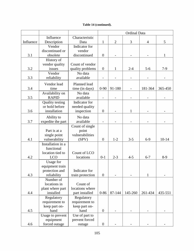
105
Table 14 (continued).
Ordinal Data
Influence Influence
Description Characteristic
Data 1 2 3 4 5
3.1
Vendor discontinued or
obsolete
Indicator for vendor
discontinued 0 - - - 1
3.2
History of vendor quality
issues Count of vendor quality problems 0 1 2-4 5-6 7-9
3.3 Vendor
reliability No data available - - - - -
3.4 Vendor lead
time Planned lead time (in days) 0-90 91-180 - 181-364 365-450
3.5 Availability on
RAPID No data available - - - - -
3.6
Quality testing or hold before
installation
Indicator for needed quality
inspection 0 - 1 - -
3.7 Ability to
expedite the part No data available - - - - -
4.1
Part is at a single point vulnerability
Count of single point
vulnerabilities (SPV) 0 1-2 3-5 6-9 10-14
4.2
Installation in a functional
location tied to LCO
Count of LCO locations 0-1 2-3 4-5 6-7 8-9
4.3
Usage for equipment train protection and
reliability Indicator for
train protection 0 - - 1 -
4.4
Number of locations in
plant where part installed
Count of locations where
part installed 0-86 87-144 145-260 261-434 435-551
4.5
Regulatory requirement to keep part on-
hand
Regulatory requirement to keep part on-
hand 0 - - - -
4.6
Usage to prevent equipment
forced outage
Use of part to prevent forced
outage 0 - - - -
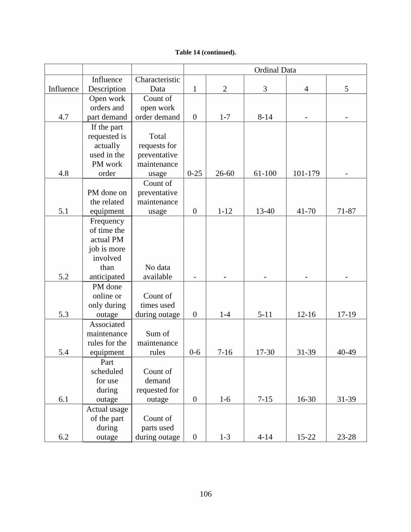
106
Table 14 (continued).
Ordinal Data
Influence Influence
Description Characteristic
Data 1 2 3 4 5
4.7
Open work orders and
part demand
Count of open work
order demand 0 1-7 8-14 - -
4.8
If the part requested is
actually used in the PM work
order
Total requests for preventative maintenance
usage 0-25 26-60 61-100 101-179 -
5.1
PM done on the related equipment
Count of preventative maintenance
usage 0 1-12 13-40 41-70 71-87
5.2
Frequency of time the actual PM job is more involved
than anticipated
No data available - - - - -
5.3
PM done online or
only during outage
Count of times used
during outage 0 1-4 5-11 12-16 17-19
5.4
Associated maintenance rules for the equipment
Sum of maintenance
rules 0-6 7-16 17-30 31-39 40-49
6.1
Part scheduled
for use during outage
Count of demand
requested for outage 0 1-6 7-15 16-30 31-39
6.2
Actual usage of the part
during outage
Count of parts used
during outage 0 1-3 4-14 15-22 23-28

107
Table 14 (continued).
Ordinal Data
Influence Influence
Description Characteristic
Data 1 2 3 4 5
6.3
When the part can be used or
equipment accessed
Indicator for using part only during outage 0 - 1 - -
7.1
Cost of expediting the
part
Total expediting
costs 0 1-200 201-1000 - -
7.2
Cost of replacement
power
Possible revenue loss
due to shutdown (in
millions) 0 0.01-39.5 39.6-118.7 118.8-197 197.1-251
The two examples above indicate that the assignment of historical part data characteristic
values to the ordinal scale is unique and may not always be linear. Some influences, such as 4.2,
follow a linear assignment, but such an assignment is not required. The main goal of the ordinal
scale is to capture the importance of the ensuing consequences if a part is not available in
inventory when required. Considering consequences in the context of each influence results in a
measure of the criticality of keeping a part in inventory. The weights assigned to each influence
then scale the criticality in the context of the overall spare parts problem.
In general, the assignment of these data to the ordinal 1-5 scale can be somewhat
qualitative and dependent on the historical values stored in the ERP system or source of part
data. These assignments are based on the perceived consequences if a part is not available when
requested from inventory. Although they are tied to potential lost revenue associated with a
situation that compromises safety at the plant and leads to possible shutdown or derate, these
perceptions could be subjective. Therefore, these scales can and should be periodically revisited
to ensure both the current part data is effectively being captured by the ordinal scale and also that

108
the most recent data available is being used to evaluate part characteristics. In this research, data
from June 2003 to February 2010 was extracted from the ERP system for the sample set of parts
provided by the test bed company. Examining a large time window allows for accurate
representation of part behavior and demand usage in the spare parts process. Spare parts
demands are extremely intermittent, and a large time window is needed to capture all relevant
information. The examination of the data for each characteristic led to assignment of historical
part data characteristic values to the ordinal scale for every influence.
Finally, it is worth mentioning that the ERP system at the test bed company currently
does not track part characteristic data related to every influence. In fact, no relevant data exists
for some influences, such as influence 2.3: Surveillance Maintenance Results. A complete
listing of influences for which no characteristic data exists can be found in Table 14, denoted by
“No data available” in the “Characteristic Data” column. For these influences, a value of 0 was
used for the part data for every part. Doing so distinguishes the lack of available data from the
ordinal scale values. If a scale value was used, a level of criticality or importance may be
assumed for that influence. Such an assumption would be misleading, as no data currently exists
for that influence. We recommend that the test bed company begins to track appropriate part
characteristic data for the influences in Table 14 and incorporate the data into the scoring
formulas to increase the accuracy of the part criticality scores.
The goal of the influence diagram and subsequent item criticality scoring is to develop a
spare parts inventory management system and reduce uncertainty in part classification and
inventory management. The influence diagram process (Chapter 3) allows companies to discern
the problem under consideration. This process may uncover some factors that are important and
relevant but do not have corresponding part data in the company’s system. It is still important to
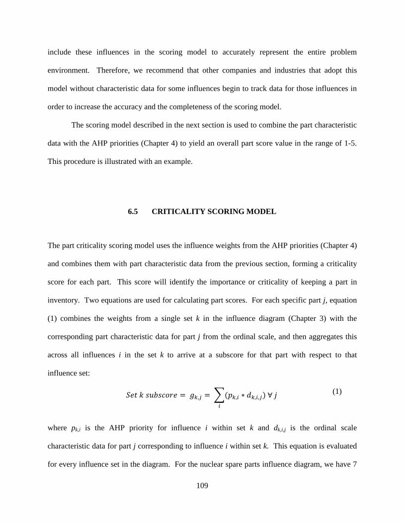
109
include these influences in the scoring model to accurately represent the entire problem
environment. Therefore, we recommend that other companies and industries that adopt this
model without characteristic data for some influences begin to track data for those influences in
order to increase the accuracy and the completeness of the scoring model.
The scoring model described in the next section is used to combine the part characteristic
data with the AHP priorities (Chapter 4) to yield an overall part score value in the range of 1-5.
This procedure is illustrated with an example.
6.5 CRITICALITY SCORING MODEL
The part criticality scoring model uses the influence weights from the AHP priorities (Chapter 4)
and combines them with part characteristic data from the previous section, forming a criticality
score for each part. This score will identify the importance or criticality of keeping a part in
inventory. Two equations are used for calculating part scores. For each specific part j, equation
(1) combines the weights from a single set k in the influence diagram (Chapter 3) with the
corresponding part characteristic data for part j from the ordinal scale, and then aggregates this
across all influences i in the set k to arrive at a subscore for that part with respect to that
influence set:
𝑆𝑒𝑡 𝑘 𝑠𝑢𝑏𝑠𝑐𝑜𝑟𝑒 = 𝑔𝑘,𝑗 = �(𝑝𝑘,𝑖 ∗ 𝑑𝑘,𝑖,𝑗) ∀ 𝑗 𝑖
(1)
where pk,i is the AHP priority for influence i within set k and dk,i,j is the ordinal scale
characteristic data for part j corresponding to influence i within set k. This equation is evaluated
for every influence set in the diagram. For the nuclear spare parts influence diagram, we have 7
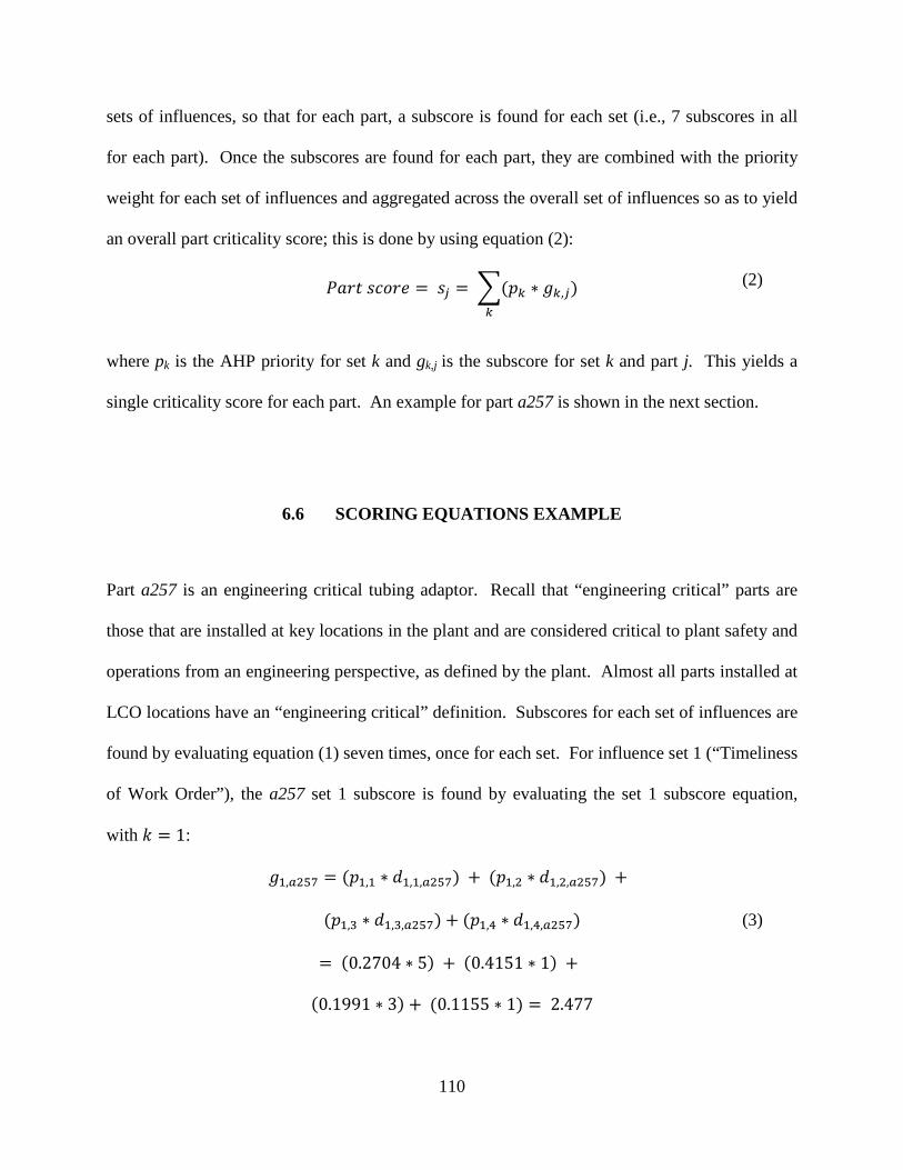
110
sets of influences, so that for each part, a subscore is found for each set (i.e., 7 subscores in all
for each part). Once the subscores are found for each part, they are combined with the priority
weight for each set of influences and aggregated across the overall set of influences so as to yield
an overall part criticality score; this is done by using equation (2):
𝑃𝑎𝑟𝑡 𝑠𝑐𝑜𝑟𝑒 = 𝑠𝑗 = �(𝑝𝑘 ∗ 𝑔𝑘,𝑗𝑘
) (2)
where pk is the AHP priority for set k and gk,j is the subscore for set k and part j. This yields a
single criticality score for each part. An example for part a257 is shown in the next section.
6.6 SCORING EQUATIONS EXAMPLE
Part a257 is an engineering critical tubing adaptor. Recall that “engineering critical” parts are
those that are installed at key locations in the plant and are considered critical to plant safety and
operations from an engineering perspective, as defined by the plant. Almost all parts installed at
LCO locations have an “engineering critical” definition. Subscores for each set of influences are
found by evaluating equation (1) seven times, once for each set. For influence set 1 (“Timeliness
of Work Order”), the a257 set 1 subscore is found by evaluating the set 1 subscore equation,
with 𝑘 = 1:
𝑔1,𝑎257 = (𝑝1,1 ∗ 𝑑1,1,𝑎257) + (𝑝1,2 ∗ 𝑑1,2,𝑎257) +
(𝑝1,3 ∗ 𝑑1,3,𝑎257) + (𝑝1,4 ∗ 𝑑1,4,𝑎257)
= (0.2704 ∗ 5) + (0.4151 ∗ 1) +
(0.1991 ∗ 3) + (0.1155 ∗ 1) = 2.477
(3)

111
Thus, each AHP priority in the “Timeliness of Work Order” set is combined with the
corresponding ordinal part characteristic scale data for each of the four influences in the set. In a
similar fashion, the subscores for sets 2-7 are found:
𝑔2,𝑎257 = (0.4006 ∗ 1) + (0.0830 ∗ 0) + (0.2375 ∗ 0)
+ (0.0915 ∗ 1) + (0.1281 ∗ 5) + (0.0593 ∗ 0) = 1.1326
(4)
𝑔3,𝑎257 = (0.4566 ∗ 1) + (0.0841 ∗ 1) + (0.1041 ∗ 0)
+ (0.1102 ∗ 4) + (0.1345 ∗ 0) + (0.0402 ∗ 1) + (0.0704 ∗ 0)
= 1.0217
(5)
𝑔4,𝑎257 = (0.3172 ∗ 1) + (0.1693 ∗ 1) + (0.1668 ∗ 1)
+ (0.0448 ∗ 1) + (0.1065 ∗ 1) + (0.1242 ∗ 1)
+ (0.0334 ∗ 1) + (0.0377 ∗ 1) = 1.0000
(6)
𝑔5,𝑎257 = (0.4855 ∗ 1) + (0.1951 ∗ 0) + (0.0941 ∗ 1)
+ (0.2252 ∗ 1) = 0.8048
(7)
𝑔6,𝑎257 = (0.4074 ∗ 1) + (0.4636 ∗ 1) + (0.1290 ∗ 1) = 1.0000 (8)
𝑔7,𝑎257 = (0.1722 ∗ 1) + (0.8278 ∗ 1) = 1.0000 (9)
The 7 subscores are then combined with the overall influence set AHP priority weights to
evaluate a final criticality score for part a257:
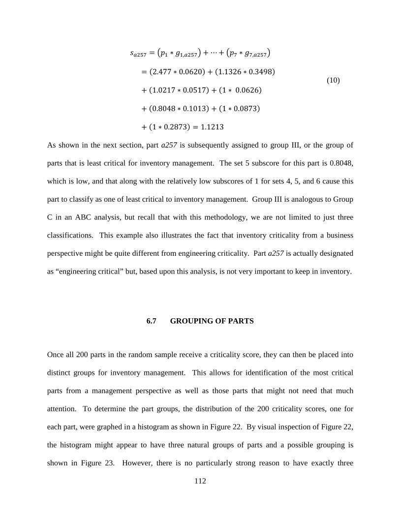
112
𝑠𝑎257 = �𝑝1 ∗ 𝑔1,𝑎257� + ⋯+ �𝑝7 ∗ 𝑔7,𝑎257�
= (2.477 ∗ 0.0620) + (1.1326 ∗ 0.3498)
+ (1.0217 ∗ 0.0517) + (1 ∗ 0.0626)
+ (0.8048 ∗ 0.1013) + (1 ∗ 0.0873)
+ (1 ∗ 0.2873) = 1.1213
(10)
As shown in the next section, part a257 is subsequently assigned to group III, or the group of
parts that is least critical for inventory management. The set 5 subscore for this part is 0.8048,
which is low, and that along with the relatively low subscores of 1 for sets 4, 5, and 6 cause this
part to classify as one of least critical to inventory management. Group III is analogous to Group
C in an ABC analysis, but recall that with this methodology, we are not limited to just three
classifications. This example also illustrates the fact that inventory criticality from a business
perspective might be quite different from engineering criticality. Part a257 is actually designated
as “engineering critical” but, based upon this analysis, is not very important to keep in inventory.
6.7 GROUPING OF PARTS
Once all 200 parts in the random sample receive a criticality score, they can then be placed into
distinct groups for inventory management. This allows for identification of the most critical
parts from a management perspective as well as those parts that might not need that much
attention. To determine the part groups, the distribution of the 200 criticality scores, one for
each part, were graphed in a histogram as shown in Figure 22. By visual inspection of Figure 22,
the histogram might appear to have three natural groups of parts and a possible grouping is
shown in Figure 23. However, there is no particularly strong reason to have exactly three
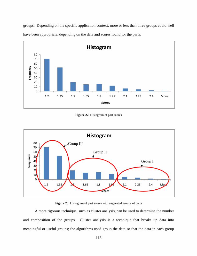
113
groups. Depending on the specific application context, more or less than three groups could well
have been appropriate, depending on the data and scores found for the parts.
Figure 22. Histogram of part scores
Figure 23. Histogram of part scores with suggested groups of parts
A more rigorous technique, such as cluster analysis, can be used to determine the number
and composition of the groups. Cluster analysis is a technique that breaks up data into
meaningful or useful groups; the algorithms used group the data so that the data in each group
01020304050607080
1.2 1.35 1.5 1.65 1.8 1.95 2.1 2.25 2.4 More
Freq
uenc
y
Scores
Histogram
01020304050607080
1.2 1.35 1.5 1.65 1.8 1.95 2.1 2.25 2.4 More
Freq
uenc
y
Scores
Histogram
Group I
Group II
Group III

114
have common characteristics and are distinct from characteristics in other groups (Tan,
Steinbach, & Kumar, 2006). One common algorithm used in cluster analysis is k-means, which
groups data by distance to centroids into a number of pre-specified groups. The algorithm tests
the absolute value of the differences between a data point and all centroids, or means, and
assigns that data point to the group whose absolute distance to the mean is minimal. The
algorithm assigns all points, calculates a new mean of each group, and repeats until the new
calculated mean is equal to the previous mean for all groups. For further details on the k-means
algorithm and cluster analysis, see Tan, Steinbach, and Kumar (2006).
Three centroids were arbitrarily chosen to seed the k-means algorithm for the part
criticality score data, as the histogram appeared to have three natural groups. Because the
algorithm is sensitive to the starting centroid values, various combinations of starting centroids
were tested with the data. Table 15 shows 15 different trials with randomly selected centroids
and the resulting number of parts placed in each group. Patterns in the results emerged, and most
trials yielded approximately 20 parts in group I, approximately 40 parts in group II, and
approximately 140 parts in group III. These similar results provide empirical evidence in
support of the natural group boundaries. Therefore, Row 13 in Table 15 was selected as the final
grouping analysis; the algorithm ran 10 iterations for this combination. Table 16 presents
descriptive statistics for each group of parts, after the final k-means cluster analysis. Parts with a
criticality score of 1.8582 or higher were placed in group I (highest criticality scores, 21 parts);
from the remaining parts, those with a criticality score of 1.4612 or higher were placed in group
II (moderate criticality scores, 38 parts); the rest of the parts were placed in group III (lowest
criticality scores, 141 parts). The cutoff scores for each group ensure the same number of parts
in each group as designated by the k-means algorithm are in the actual criticality groups.
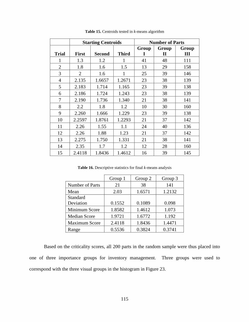
115
Table 15. Centroids tested in k-means algorithm
Starting Centroids Number of Parts
Trial First Second Third Group
I Group
II Group
III 1 1.3 1.2 1 41 48 111 2 1.8 1.6 1.5 13 29 158 3 2 1.6 1 25 39 146 4 2.135 1.6657 1.2671 23 38 139 5 2.183 1.714 1.165 23 39 138 6 2.186 1.724 1.243 23 38 139 7 2.190 1.736 1.340 21 38 141 8 2.2 1.8 1.2 10 30 160 9 2.260 1.666 1.229 23 39 138 10 2.2597 1.8761 1.2293 21 37 142 11 2.26 1.55 1.1 24 40 136 12 2.26 1.88 1.23 21 37 142 13 2.275 1.750 1.331 21 38 141 14 2.35 1.7 1.2 12 28 160 15 2.4118 1.8436 1.4612 16 39 145
Table 16. Descriptive statistics for final k-means analysis
Group 1 Group 2 Group 3
Number of Parts 21 38 141 Mean 2.03 1.6571 1.2132 Standard Deviation 0.1552 0.1089 0.098 Minimum Score 1.8582 1.4612 1.073 Median Score 1.9721 1.6772 1.192 Maximum Score 2.4118 1.8436 1.4471 Range 0.5536 0.3824 0.3741
Based on the criticality scores, all 200 parts in the random sample were thus placed into
one of three importance groups for inventory management. Three groups were used to
correspond with the three visual groups in the histogram in Figure 23.
116
6.8 VALIDATION
Supply chain analysts at the test bed facility validated the completeness of the sample set of part
data, ensuring all relevant history and work order data was pulled from the ERP system for the
200 parts in the sample set over the historical window. Four supply chain analysts and one
engineer verified the availability of data for each of the influences and ensured the correct data in
the ERP system were used as the most representative data for each influence. Those analysts
also verified that data are not available or currently tracked for the influences marked as such in
Table 14.
The cutoffs between each group of parts were also validated. Analysts at the test bed
company received a list of parts whose criticality scores were close to the breakpoints between
each group of parts—I, II and III. Thus, the list contained parts that were around the score
breakpoint between group I and group II and parts that were around the score breakpoint
between group II and group III. The list also included a couple of parts in each group that were
not around the score breakpoints. It was then verified with the analysts that the resulting part
grouping was reasonable in terms of inventory criticality.
6.9 SUMMARY
This chapter presents a method for grouping parts for inventory management based on part
criticality scores. The methodology is illustrated using actual characteristic data for spare parts
from the test bed company ERP system. The criticality scores that are developed are
comprehensive, because all relative influences to the spare parts management process are

117
represented in the criticality scores. The part criticality scores can then be used to identify
groups for inventory management, so that the appropriate amount of time and resources can be
expended on each part. The scores should be periodically updated to ensure accurate
representation of actual part usage, by using updated part data from the ERP system and
reevaluating both the scoring equations and k-means clustering algorithm. The scores should
also be updated as more data becomes available, especially data for influences that are not
currently tracked in the ERP system. Periodically revisiting the criticality scores will ensure the
corresponding inventory policy is flexible, responsive, accurate, and robust. The next chapter
discusses appropriate inventory management policies for each group of parts.

118
7.0 INVENTORY MANAGEMENT POLICY
The previous chapter discussed the criticality scoring method for spare parts and described how
the parts can be placed into groups for inventory management based on both influence rankings
by the subject matter experts (SMEs) and part characteristic data. This chapter details the
analysis used to determine appropriate parameters for an inventory policy for each group of parts
(I, II, and III). A modified base stock policy is used, trading off costs of inventory investments
against delays in work due to lack of parts (stockouts); this tradeoff is examined, quantified, and
analyzed in this chapter. In the case of the test bed company, the exact costs of delaying work
cannot be completely determined, but clearly the costs drive the problem. A retrospective
(historical) numerical simulation approach is used to determine the base stock reorder point. We
begin with a brief discussion of common inventory control systems including base stock policies.
7.1 COMMON INVENTORY SYSTEMS
Inventory control systems determine what to order, when to order, and how much to order.
Periodic review models, or fixed interval systems, review inventory levels periodically at
specified intervals (the review interval), and an order is placed if the stock level is at or below
some reorder point during review. The amount ordered (Q) is equal to the desired inventory
position less the current inventory position. Because the order is based on an order-up-to
119
amount, the amount Q can change with each order. On the other hand, continuous review
models constantly monitor inventory levels (i.e., the review interval is equal to zero), and orders
could be placed at any time, not just at predefined elapsed time intervals. The size of an order
can be determined by various methods, including, but not limited to, the economic order quantity
(EOQ) and its variants, production order quantity, quantity discount based models, and single
period models (Heizer & Render, 2011). Probabilistic models also consider expected demand
during the lead time and place orders when the stock level is equal to a reorder point plus some
safety stock. Continuous review models are commonly called (Q, R) systems, where Q
represents the pre-set order amount and R represents the reorder point (ROP), signifying an order
of Q units when the inventory position reaches R units. The main distinction between periodic
and continuous review models is that periodic models order varying amounts at set times, while
continuous review models typically order set amounts at varied times. For further details on
these models, see Nahmias (2005), Heizer and Render (2011), Hopp and Spearman (2001), and
Krajewski and Ritzman (2005).
A special case of a continuous review model is a base stock system for inventory
management. Base stock systems utilize one-for-one replenishment and place a replenishment
order for the exact amount demanded at the time of demand. The base stock system maintains an
inventory position equal to the expected demand during lead time plus some safety stock (which
is the same calculation as ROP in a (Q, R) system (Krajewski & Ritzman, 2005)), and the base
stock levels set a desired inventory position that can be determined either by minimizing a total
expected cost function or specifying a service level. However, order quantities vary in base
stock systems, and order frequency is typically greater than that of a (Q, R) system. More orders
tend to be placed in smaller amounts. Krajewski and Ritzman (2005) argue that base stock

120
models are most appropriate for very expensive items as well as just-in-time kanban systems.
Further description of base stock systems can be found in both Hopp and Spearman (2001) and
Krajewski and Ritzman (2005).
Because nuclear spare parts can be both expensive and highly critical to plant operations,
a base stock system is especially appropriate for managing inventory of these parts.
Furthermore, lead time for nuclear spare parts can be substantial (exceeding 200 days for some
parts), so a base stock system that considers demand during lead time while minimizing
inventory held in stock is fitting; no more inventory is held than the expected demand during
lead time plus some safety stock. Minimizing on-shelf inventory is important, because nuclear
spare parts are very expensive, and recovery of the costs of the parts is not guaranteed in a
deregulated environment. Furthermore, purchased parts usually cannot be returned to the vendor
because they are often customized to the nuclear facility. A base stock policy tends to be
conservative, which aligns well with the risk averse and conservative nuclear culture, as
discussed in Chapter 2.
However, difficulty using a base stock system can arise due to the challenges of
accurately characterizing lead time demand. As shown in the next section, this is unfortunately
the case with nuclear spare parts; in particular, the sample of parts examined in this dissertation
falls into this category. In such situations, a different approach must be used to determine the
base stock inventory position. In this research, a retrospective numerical simulation is developed
to arrive at such a policy. The approach modifies the traditional base stock policy by considering
various multiples of an average part request at the plant as the desired base stock inventory
position. The analysis examines the tradeoff between increased dollar investment in inventory
against delays incurred in maintenance or repair due to unavailability of parts. The tradeoff can
121
be examined by management and applied to make decisions that align with their own tolerance
for risk, as cost consequences and corresponding risk of delayed maintenance are associated with
each policy.
7.2 LEAD TIME ANALYSIS
Traditional inventory models are driven by lead time and demand during lead time. Stockouts
before the next order arrives result in lost or delayed sales; in the case of spare parts, stockouts
can lead to offlining of a production process. The key is to prevent stockouts by ensuring that
enough inventory is on the shelf to cover demand during the elapsed time between placement of
an order and its receipt from the vendor. Probabilistic inventory models require a distribution of
demand during the lead time in order to compute the optimal ROP. However, obtaining this
distribution is not always possible; as discussed in Chapter 2, demand for nuclear spare parts is
highly intermittent and confounded by returns from the plant to the warehouse. Traditional
forecasting models do not work for these data, and failure rates do not exist. It is thus impossible
to develop a well-defined distribution of demand. In this research, an attempt was made to
obtain a distribution, regardless of the challenges, by using a rolling time window approach to
determine demand during the lead time.
This approach tallies plant demands less plant returns over rolling time windows, each of
length equal to the lead time, for each part over a historical time window. For example, if part D
has a lead time of 90 days and the historical time window of previous demand data is 2 years, the
first rolling window would calculate net demand (warehouse issues in response to plant requests
less plant returns to warehouse) over days 1 to 90, the second window would calculate net

122
demand over days 2 to 91, the third window would calculate net demand over days 3 to 92, and
so on, until the final window to calculate net demand over days 641 to 730 (= 365 days/year
times 2 years). Recall that plant returns to the warehouse are important to remove from the
demand calculation because returns indicate false demand signals and do not represent actual
plant usage. A histogram can then be plotted of the net demands over each lead time window to
determine a distribution of demand during the lead time.
The lead time rolling window analysis was done for each of the 200 spare parts in the
random sample of parts discussed in Chapter 6. The historical window covered June 1, 2003 to
July 31, 2010, and all demands and return data for the 200 parts in the random sample were
extracted from the test bed company’s Enterprise Resource Planning (ERP) system. Histograms
for demand during respective lead times for three example parts are shown in Figure 24, Figure
25, and Figure 26.
Figure 24. Lead time histogram for part a250
0 1
338480
1254
6
270
0 00
200
400
600
800
1000
1200
1400
-3 -2 -1 0 1 2 3 4 More
Num
ber o
f occ
urre
nces
Net demand in lead time window (issues - returns)
Histogram for Part a250

123
Figure 25. Lead time histogram for part b166
Figure 26. Lead time histogram for part a65
Figure 24 is the lead time demand distribution histogram for part a250 (level switch) with
a lead time of 270 days. From the histogram, no obvious distribution or demand pattern can be
discerned for the lead time data. Figure 24 also shows returns confounding the results; there
were 338 instances of (-1) demand during lead time, meaning a net return of one unit occurred
multiple times over the rolling lead time intervals in the historical data. Positive demands did
0
2563
28 140
500
1000
1500
2000
2500
3000
-1 0 1 More
Num
ber o
f occ
urre
nces
Net demand in lead time window (issues - returns)
Histogram for Part b166
2535
0 0 41 0 0 0 0 0 0 0 0 0 0 0 0 0 0 0 0 1 00
500
1000
1500
2000
2500
3000
0 5 10 15 20 25 30 35 40 45 50 55 60 65 70 75 80 85 90 95 100
Mor
e
Num
ber o
f occ
urre
nces
Net demand in lead time window (issues - returns)
Histogram for Part a65

124
exist, clearly more often than periods of zero demand, but some of those positive demands were
cancelled out by the later return of parts to the warehouse. Figure 25 presents the histogram for
part b166 (spiral wound gasket), with a lead time of 14 days. Rarely does positive demand occur
during this part’s historical window. In fact, only 42 lead time windows have positive demand;
this is shown by the labels on each bar of the histogram, which are a count of the number of
occurrences of net demand during the lead time window. No distribution can be determined
from these data. Finally, Figure 26 shows the histogram for part a65 (washer), with a lead time
of 42 days. Once again, rolling lead time windows with zero demand are prevalent; occasionally
positive demand exists but with no pattern or clear distribution to the data. Similar results were
obtained for other parts in the random sample; no distributions of demand could be deduced from
the histograms.
In summary, a distribution for demand during the lead time cannot be determined for
these data, as there are no discernable patterns in the histograms. Furthermore, even the shapes
of the histograms for parts in the same criticality group are different. Figure 24, Figure 25, and
Figure 26 are three parts from group I—most inventory critical. Clearly the histograms for these
parts do not have consistent results or patterns.
Thus, because a base stock system requires a distribution for demand during the lead
time, the traditional policy must be modified in order to develop an inventory management
system that supports the criticality definition of every group of parts. Recall that a base stock
policy aims to minimize on hand inventory by stocking no more than expected demand during
lead time plus an appropriate amount of safety stock. To modify the base stock system, a
retrospective numerical simulation is developed to evaluate various multiples of average demand
per plant request as potential base stock inventory positions. This simulation attempts to

125
minimize inventory investment (akin to minimizing inventory on hand) by using proxies
(multiples of average demand per plant request) for expected demand during lead time. Further
details of the simulation are given in the next section.
7.3 HISTORICAL SIMULATION
The simulation used to determine corresponding inventory policies for each group of parts uses
historical demands and returns. A probability distribution for demand, as is traditionally used in
simulation, is not considered in this study. Demand and return data for the random sample of
200 parts were extracted from the test bed company’s ERP system for the period between June 1,
2003 and July 31, 2010. Using historical demands assumes the past represents the future; this is
reasonable because no reason or evidence exists to suggest that demand will not continue to be
intermittent in the future.
The simulation was written in MATLAB, and the code can be found in Appendices C.1,
C.2, and C.3. The simulation employs the described modified base stock policy, reading in files
of part demand and return data, part lead time, cost of parts, and part demands at limited
condition of operation (LCO) locations. Recall that failure of a part at an LCO location can lead
to plant shutdown, usually in 72 hours, if the situation is not remedied. A lower and an upper
bound for base stock inventory position as a multiple of mean demand per plant request are
specified by the user. For this analysis, the base stock lower bound was initialized at 0 and the
multiplier is incremented in units of 0.5 until reaching an upper bound of 50, i.e., corresponding
to a base stock that is 5000% of the mean demand per plant request. Such a high upper bound
was used to determine the level of on shelf inventory required to ensure that no work orders

126
would ever be delayed due to lack of parts, in essence maintaining a 100% service rate. Thus,
inventory positions 𝐼𝑃𝑏,𝑘 = 𝑏 ∗ 𝑧𝑘 were considered for 101 unique values of 𝑏 = 0, 0.5,1, … , 50,
where b is a multiplier for the mean effective demand per plant request, and 𝑧𝑘, 𝑘 = 1, 2, … , 200,
is the average demand per plant request for part k over the historical window. As an example, if
the average demand of part k = 1 over the historical window was 𝑧1 = 5 units per order, the
lower bound for inventory position would be 𝐼𝑃0,1 = 𝑏 ∗ 𝑧1 = 0.0(5) = 0 and the upper bound
would be 𝐼𝑃50,1 = 𝑏 ∗ 𝑧1 = 50.0(5) = 250. In the case of decimal values for inventory position,
such as 𝐼𝑃0.5,1 = 𝑏 ∗ 𝑧1 = 0.5(5) = 2.5, the ceiling of the inventory position is always taken, in
this case, always rounding up 2.5 to 3.0. The simulation runs 101 times, once with each value of
b. Note that b = 0.0 is an extreme case and represents holding zero inventories on the shelf.
This instance of holding nothing will always cause delayed days for every plant demand request
because no inventory is held on the shelf to satisfy the next request. In practice, such a policy
would not be implemented; however, it is included as an extreme instance for the sake of
completeness.
The historical window of part demand and return data ranged from June 1, 2003 to July
31, 2010, which constituted 2,618 days. Therefore, for each of the 101 values of b, the
simulation carries out 2,618 days of historical issues and returns between the warehouse and the
plant. Starting inventory is equal to the previous ending day’s inventory, except for day 1, where
starting inventory is equal to the base stock inventory position 𝐼𝑃𝑏,𝑘. A day’s ending inventory
𝐼𝑗,𝑘 for a part k is calculated in the following manner:
𝐼𝑗,𝑘 = 𝑠𝑗,𝑘 + 𝑎𝑗,𝑘 + 𝑟𝑗,𝑘 − 𝑑𝑗,𝑘 (11)

127
where 𝑠𝑗,𝑘 denotes the starting inventory on the shelf at the beginning of day j for part k, 𝑎𝑗,𝑘 is
the quantity received in order arrivals from the vendor on day j for part k, 𝑟𝑗,𝑘 is the amount of
returns from the plant on day j for part k, and 𝑑𝑗,𝑘 is the amount of part k issued to the plant on
day j. Orders are placed if 𝐼𝑗,𝑘 ≤ 𝐼𝑃𝑏,𝑘 and 𝑑𝑗,𝑘 > 0. The order amount 𝑚𝑗,𝑘 is defined as
𝑚𝑗,𝑘 = 𝑑𝑗,𝑘 − 𝑟𝑗,𝑘. Note that additional returns could raise the on-shelf ending inventory
position 𝐼𝑗,𝑘 greater than the desired base stock inventory position 𝐼𝑃𝑏,𝑘. In such cases, no orders
are placed until 𝐼𝑗,𝑘 < 𝐼𝑃𝑏,𝑘. An order that is placed is scheduled to arrive after the part’s lead
time, and order costs are charged. Holding costs per day are charged to the day’s ending
inventory.
If sufficient inventory is not on the shelf to satisfy demand, a delayed work day is
charged, with tracking for occurrence at an LCO or non-LCO location. The simulation stores
this information in an output file along with total part capital costs for all purchased parts in the
group over the historical window. A second output file stores the total cost of on-shelf base
stock inventory for all parts in the criticality group. A third file stores the base stock inventory
costs broken down individually by part and value of b. Ordering and holding costs were
extremely small in our particular application and are ignored in the overall calculation.
7.4 CALCULATING AVERAGE EFFECTIVE DEMAND PER PLANT REQUEST
In order to determine the optimal base stock inventory position for a part 𝐼𝑃𝑏,𝑘, multiples of
average effective demand per plant request b are tested over the historical data window. The
calculation of average effective demand is not straightforward because it is confounded by

128
returns. In the sample data received from the test bed company, the return data cannot be
matched to the original demand data. The data from the ERP system lists plant demands and
returns from the plant to the warehouse but does not specify which particular request resulted in
a return. For example, over the historical window, if part E had three instances of plant requests
for 2 units each, and two returns of 1 unit each, the data from the ERP at the test bed company
system would show three data entries of demand and two data entries of returns. The data would
not list which of the original demands were returned. The two returns could be from two
separate original requests (thus implying that half of the original order (1 of 2 parts) was returned
two separate times) or the two returns could be from a single original demand, with half of the
original order sent back on one occasion and half sent back on another occasion, completely
cancelling out the original demand. There is no way to know how the demands match up with
returns based on the data tracked by the test bed company.
An accurate calculation of average demand per plant request for part k, 𝑧𝑘, would first
subtract all returns to the warehouse from the total amount demanded by the plant and then find
the average across all demands. However, as noted, accurately matching up every return with its
corresponding demand is impossible.
To illustrate the possibilities for returns, consider the example in Table 17, a hypothetical
six period window for part F with issues to and returns from the plant as shown.
Table 17. Hypothetical movement data for part F
Time Period Movement
Number of Parts
1 Issue to plant 4 2 Issue to plant 1 3 Issue to plant 2 4 Return from plant 2 5 Return from plant 1 6 Issue to plant 2

129
There are many possible combinations for how the returns in periods 4 and 5 could match with
the issues to the plant. For example, the 2 units returned in period 4 could correspond to the 2
units issued in period 3, thus cancelling out the entire demand in that period. The same 2 units
could also match up with the issues in period 1, reducing but not totally cancelling out the
demands in that period. The two returned units could also be split, matching one unit with one
previous issue and another unit with another previous issue. Similarly, the 1 unit of return in
period 5 could completely cancel the demand in period 2 or reduce the overall demand in periods
1 or 3. Clearly, enumerating all possible issue and return combinations for multiple part
transactions is not practical. So, we consider two extremes when calculating average demand:
(1) never adjusting any demand occasions for returns (which would underestimate average
demand) and (2) adjusting demand occasions for all returns (which would overestimate average
demand). This calculation of bounds for average demand per plant request, 𝑧𝑘, along with the
calculation of an intermediate value, is illustrated in the following example.
7.4.1 Calculating the Lower Bound of zk
The lower bound of 𝑧𝑘 calculates average demand while never adjusting for returns. This
assumes that returns never completely cancel out an entire issue to the plant. In this case, for the
data in Table 17, 𝑧𝐹 =(∑ 𝑑𝑗,𝐹)−(∑ 𝑟𝑗,𝐹
6𝑗=1 )6
𝑗=1
∑ 𝑐𝑑𝑗,𝐹6𝑗=1
= 9−34
= 1.5, where 𝑐𝑑𝑗,𝑘 is an indicator variable
representing the occurrence of an issue of part k to the plant on day j. There are four issues in the
hypothetical movement data, so ∑ 𝑐𝑑𝑗,𝐹6𝑗=1 = 4. The number of return instances is not
considered, i.e., it is assumed that no return instance ever cancels all demand for even one
demand instance. This equation uses the largest possible denominator for the average demand

130
calculation, and by dividing by the largest possible number, average demand per request from the
plant is underestimated. This is a lower bound, thus the average demand cannot be smaller than
this value. We now look at adjusting for all returns in the count of demands.
7.4.2 Calculating the Upper Bound of zk
The upper bound of 𝑧𝑘 calculates average demand while always adjusting for returns. In this
case, for the data in Table 17, 𝑧𝐹 =(∑ 𝑑𝑗,𝐹)−(∑ 𝑟𝑗,𝐹
6𝑗=1 )6
𝑗=1
∑ 𝑐𝑑𝑗,𝐹6𝑗=1 −∑ 𝑐𝑟𝑗,𝐹
6𝑗=1
= 9−34−2
= 3, where 𝑐𝑟𝑗,𝑘 is an indicator
variable representing the occurrence of a return of part k to the plant on day j. The equation for
lower bound uses the smallest possible denominator for the average demand calculation and
assumes an instance of a return always entirely cancels out an instance of demand. Thus, every
return instance is considered in the denominator. Dividing by the smallest possible number
yields an overestimation of average demand per plant request.
In reality, the count of the number of instances of demand requests from the plant most
likely falls in between the overestimations and underestimations of demand. Sometimes a return
completely cancels out a demand instance, and sometimes it does not. This situation is
considered next.
7.4.3 Calculating an Intermediate Value of zk
To find a point in the range between the underestimation and overestimation of 𝑧𝑘, we consider
only half of the instances of returns. With Table 17, this yields 𝑧𝐹 =(∑ 𝑑𝑗,𝐹)−(∑ 𝑟𝑗,𝐹
6𝑗=1 )6
𝑗=1
∑ 𝑐𝑑𝑗,𝐹6𝑗=1 −0.5(∑ 𝑐𝑑𝑗,𝐹
6𝑗=1 )
=
9−34−1
= 2. This calculation takes into consideration that some returns most likely do not

131
completely cancel out an original demand while other returns do completely cancel out an
original demand; 50% of return instances are considered as an average number of cancelling
occurrences. Thus, the true average demand per plant request per part falls within a range
bounded by the calculations for overestimating and underestimating demand. In this
hypothetical example, the true average falls between [1.5, 3], with 2 as an intermediate value in
this range.
Because the true value of average demand is not known, the simulation considers all
three calculations of 𝑧𝑘 for every k (lower bound, upper bound, intermediate value). Appendices
C.1, C.2 and C.3 show the corresponding simulation codes for each calculation of 𝑧𝑘. The next
section details the simulation results for the base stock inventory policy simulation.
7.5 RESULTS AND DISCUSSION
For every group of parts (I, II, and III), the simulation was run three times, once for each version
of code (lower bound, upper bound, intermediate value) corresponding to calculation of average
effective demand. For purposes of this discussion, we focus on parts in group I (most inventory
critical) and the version of code that uses an intermediate estimate of average effective demand.
The steps followed were repeated for all groups of parts and versions of code (nine total
combinations). Values of 𝑏 = 0, 0.5,1, … , 50 were considered in an attempt to reduce the missed
days to zero. Missed days occur when the plant historically demands parts, but enough inventory
does not exist on the shelf to fill the order. Missed days are calculated in total across all parts in
the group, with one tally for missed days at LCO locations and another tally for missed days at
non-LCO locations. Recall that a part failure at an LCO location forces a shutdown or derate if

132
not remedied in a prescribed amount of time (usually 72 hours). Average missed days per month
per part are then calculated by dividing total missed days by the number of months of historical
data (86 months) and then by the number of parts in the group (21 parts for group I). Figure 27
and Figure 28 show graphs for all parts in group I, depicting the cost of base stock inventory
versus average missed days per part. Average missed days for both LCO and non-LCO parts are
shown as two separate graphs. Table 18 shows the total cost to maintain the base stock inventory
positions 𝐼𝑃𝑏,𝑘 for all parts in group I for each value of b, along with corresponding average
missed LCO and non-LCO days per part per month. The table is truncated at b = 20, as the
average missed days do not improve beyond this value of b. Naturally, costs to maintain the
base stock inventory increase beyond b = 20. Clearly, the best performance occurs at b = 8.5;
average non-LCO days are minimized, average LCO days are 0, and the cost of inventory is
$669,311.50. This is the least expensive inventory policy for this group when considering all
parts in the group and aiming to minimize or eliminate all missed days due to stockout. Using
the intermediate average effective demand calculation for 𝑧𝑘, the test bed company could have
minimized the cost of base stock inventory while essentially never historically missing a work
day by setting b = 8.5 and holding 850% of 𝑧𝑘 ∀ 𝑘 in group I. Alternatively, if the company only
wants to avoid losing LCO days at all costs but is willing to tolerate some loss in non-LCO days,
a value of b = 5.5 could be used; this would have eliminated all LCO day losses and resulted in
an average of 0.254 non-LCO days lost per part per month; the base stock inventory investment
cost of this policy would have been $433,554.27. Table 18 could also be used for evaluating
other intermediate policies that are consistent with the company’s risk tolerance profile.
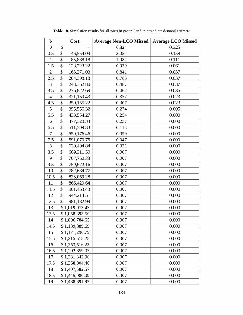
133
Table 18. Simulation results for all parts in group I and intermediate demand estimate
b Cost Average Non-LCO Missed Average LCO Missed 0 $ - 6.824 0.325
0.5 $ 46,554.09 3.054 0.158 1 $ 85,888.18 1.982 0.111
1.5 $ 128,723.22 0.939 0.061 2 $ 163,271.03 0.841 0.037
2.5 $ 204,398.18 0.788 0.037 3 $ 243,362.80 0.487 0.037
3.5 $ 276,822.69 0.462 0.035 4 $ 321,159.43 0.357 0.023
4.5 $ 359,155.22 0.307 0.023 5 $ 395,556.32 0.274 0.005
5.5 $ 433,554.27 0.254 0.000 6 $ 477,328.33 0.237 0.000
6.5 $ 511,309.33 0.113 0.000 7 $ 550,176.46 0.099 0.000
7.5 $ 591,070.75 0.047 0.000 8 $ 630,404.84 0.021 0.000
8.5 $ 669,311.50 0.007 0.000 9 $ 707,760.33 0.007 0.000
9.5 $ 750,672.16 0.007 0.000 10 $ 782,684.77 0.007 0.000
10.5 $ 823,059.28 0.007 0.000 11 $ 866,429.64 0.007 0.000
11.5 $ 901,463.43 0.007 0.000 12 $ 944,214.51 0.007 0.000
12.5 $ 981,182.99 0.007 0.000 13 $ 1,019,973.43 0.007 0.000
13.5 $ 1,058,893.50 0.007 0.000 14 $ 1,096,784.65 0.007 0.000
14.5 $ 1,139,889.69 0.007 0.000 15 $ 1,171,290.79 0.007 0.000
15.5 $ 1,215,518.28 0.007 0.000 16 $ 1,253,516.23 0.007 0.000
16.5 $ 1,292,859.03 0.007 0.000 17 $ 1,331,342.96 0.007 0.000
17.5 $ 1,368,004.46 0.007 0.000 18 $ 1,407,582.57 0.007 0.000
18.5 $ 1,445,980.09 0.007 0.000 19 $ 1,488,891.92 0.007 0.000
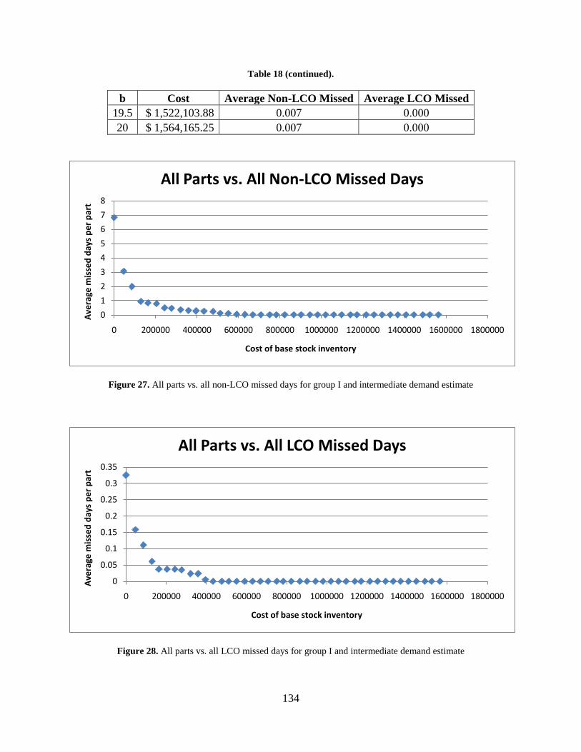
134
Table 18 (continued).
b Cost Average Non-LCO Missed Average LCO Missed 19.5 $ 1,522,103.88 0.007 0.000 20 $ 1,564,165.25 0.007 0.000
Figure 27. All parts vs. all non-LCO missed days for group I and intermediate demand estimate
Figure 28. All parts vs. all LCO missed days for group I and intermediate demand estimate
0
1
2
3
4
5
6
7
8
0 200000 400000 600000 800000 1000000 1200000 1400000 1600000 1800000
Ave
rage
mis
sed
days
per
par
t
Cost of base stock inventory
All Parts vs. All Non-LCO Missed Days
0
0.05
0.1
0.15
0.2
0.25
0.3
0.35
0 200000 400000 600000 800000 1000000 1200000 1400000 1600000 1800000
Ave
rage
mis
sed
days
per
par
t
Cost of base stock inventory
All Parts vs. All LCO Missed Days

135
7.5.1 Special Attention Parts
Most of the LCO work days delayed can be attributed to a very small subset of parts; reducing
the delayed LCO days for these parts greatly reduces the exposure to risk of offlining or derating
the plant. Adding extra parts to inventory to cover demand could yield potential savings of
millions of dollars. Depending on weather, economic conditions, size of plant, and locational
marginal prices (LMPs) of electricity, completely offlining a nuclear plant could cost between
$500,000 and $1,000,000 per day. A derate would cause some fraction of that cost, depending
on the amount of reduction in overall power output. Regardless of a full offlining or a partial
derate, the costs incurred are substantial. Thus, working to eliminate all missed days associated
with LCO locations can greatly improve the policy and its successful implementation. As an
illustration, Table 19 shows all parts from the sample of 200 parts across all criticality groups
that contribute to delayed work days at LCO locations, the criticality grouping for each part, the
number of delayed work days at LCO locations, lead time, part cost, and average effective
demand using the calculation with demand underestimated; note there are only 9 parts out of the
sample of 200. Clearly most of these 9 parts are very inexpensive, and adding more parts to
inventory would significantly reduce the exposure to risk. After further investigation, 12 parts
out of the 200 in the random sample are installed at LCO locations, and 9 of the 12 contribute to
delayed work days at LCO locations. This constitutes 75% of the parts installed at LCO
locations but only 4.5% of the overall set of parts in the random sample. Providing extra
attention to these parts and developing a modified policy for them would reduce risk exposure
and improve the overall inventory policy.
These nine parts are unique, and knowledge from a SME can be beneficial to determine
exactly how many more parts must be kept in inventory to avoid risk and reduce exposure to
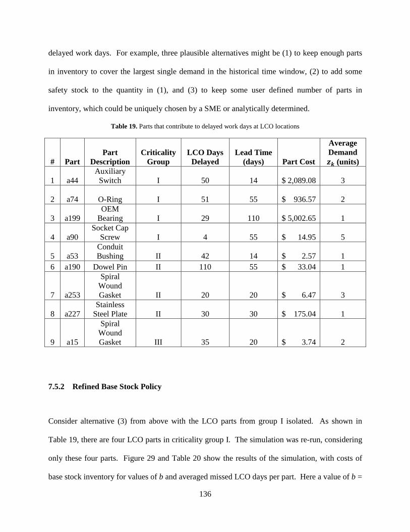
136
delayed work days. For example, three plausible alternatives might be (1) to keep enough parts
in inventory to cover the largest single demand in the historical time window, (2) to add some
safety stock to the quantity in (1), and (3) to keep some user defined number of parts in
inventory, which could be uniquely chosen by a SME or analytically determined.
Table 19. Parts that contribute to delayed work days at LCO locations
# Part Part
Description Criticality
Group LCO Days
Delayed Lead Time
(days) Part Cost
Average Demand 𝒛𝒌 (units)
1 a44 Auxiliary
Switch I 50 14 $ 2,089.08 3
2
a74 O-Ring I 51 55 $ 936.57 2
3 a199 OEM
Bearing I 29 110 $ 5,002.65 1
4 a90 Socket Cap
Screw I 4 55 $ 14.95 5
5 a53 Conduit Bushing II 42 14 $ 2.57 1
6 a190 Dowel Pin II 110 55 $ 33.04 1
7 a253
Spiral Wound Gasket II 20 20 $ 6.47 3
8 a227 Stainless
Steel Plate II 30 30 $ 175.04 1
9 a15
Spiral Wound Gasket III 35 20 $ 3.74 2
7.5.2 Refined Base Stock Policy
Consider alternative (3) from above with the LCO parts from group I isolated. As shown in
Table 19, there are four LCO parts in criticality group I. The simulation was re-run, considering
only these four parts. Figure 29 and Table 20 show the results of the simulation, with costs of
base stock inventory for values of b and averaged missed LCO days per part. Here a value of b =

137
5.5, or 550% of 𝑧𝑘 would have eliminated all LCO missed days due to part unavailability when
needed (stockout). This corresponds to a minimum of $79,503.76 in base stock inventory for
these four parts alone. The tradeoff of holding inventory clearly dominates the costs that would
be incurred if the plant had to be offlined or derated. Table 20 is truncated at b = 7, but Figure
29 shows the results up to b = 20.
Figure 29. LCO parts vs. LCO missed days for group I and intermediate demand estimate
Table 20. Simulation results for LCO parts in group I and intermediate demand estimate
b Cost Average LCO Missed 0 $ - 1.183
0.5 $ 12,281.21 0.828 1 $ 17,470.69 0.581
1.5 $ 26,726.25 0.320 2 $ 31,915.73 0.195
2.5 $ 41,171.29 0.195 3 $ 46,360.77 0.195
3.5 $ 50,613.68 0.183 4 $ 60,805.81 0.122
4.5 $ 65,058.72 0.122 5 $ 75,250.85 0.026
5.5 $ 79,503.76 0.000 6 $ 89,695.89 0.000
6.5 $ 93,948.80 0.000 7 $ 99,138.28 0.000
0
0.2
0.4
0.6
0.8
1
1.2
1.4
0 50000 100000 150000 200000 250000 300000
Ave
rage
mis
sed
days
per
par
t
Cost of base stock inventory
LCO Parts vs. LCO Missed Days

138
Clearly, if the LCO parts are isolated from the group and managed under a special policy, the
non-LCO parts could also be considered separately. Figure 30 and Table 21 show the simulation
results for just the 17 non-LCO parts in group I. Here the average missed days per part do not
improve after b = 8.5. The cost to maintain base stock inventory when b = 8.5 for these 17 parts
is $546,472.62. Note that the total cost of a separate LCO and non-LCO policy is $79,503.76 +
$546,472.62 = $625,976.38, with b = 5.5 and b = 8.5, respectively. This cost is less than the
total base stock inventory cost when considering all group I parts together, which was
$669,311.50. These costs are the minimum on hand inventory positions for the group I parts to
have essentially no delays of any kind.
Figure 30. Non-LCO parts vs. non-LCO missed days for group I and intermediate demand estimate
However, the cost of delaying work by one day at a non-LCO location is not the same as
the corresponding cost at an LCO location. While the delay costs at a non-LCO location are
difficult to determine in general, they are significantly lower than those at LCO locations.
Ideally, we would like to have values for both of these costs, but the test bed company does not
currently measure costs of delaying work at a non-LCO location. Metrics are in place to track
open work orders with the goal of minimizing work orders in the queue. Clearly, some penalty
0
2
4
6
8
10
0 200000 400000 600000 800000 1000000 1200000 1400000
Ave
rage
mis
sed
days
per
par
t
Cost of base stock inventory
Non-LCO Parts vs. Non-LCO Missed Days

139
for delaying non-LCO work must exist. If no penalty existed, no tracking would take place, and
a goal of minimizing work in the queue would be nonexistent. Attention is paid to work at non-
LCO locations; however, costs are not quantified.
Table 21. Simulation results for non-LCO parts in group I and intermediate demand estimate
b Cost Average Non-LCO Missed 0 $ - 7.660
0.5 $ 34,272.88 3.553 1 $ 68,417.49 2.252
1.5 $ 101,996.97 0.982 2 $ 131,355.30 0.933
2.5 $ 163,226.89 0.869 3 $ 197,002.03 0.496
3.5 $ 226,209.01 0.476 4 $ 260,353.62 0.375
4.5 $ 294,096.50 0.314 5 $ 320,305.47 0.314
5.5 $ 354,050.51 0.314 6 $ 387,632.44 0.293
6.5 $ 417,360.53 0.140 7 $ 451,038.18 0.122
7.5 $ 482,676.91 0.058 8 $ 516,821.52 0.026
8.5 $ 546,472.62 0.008 9 $ 579,731.97 0.008
Because costs are not quantified and some non-LCO work remains in the queue, the test
bed company may be satisfied with average missed monthly non-LCO days per part that are
somewhat larger than the minimum attainable value of 0.008. Relaxing the average missed days
would reduce the on hand base stock inventory position for all non-LCO parts in the group. For
group I, the potential for savings is substantial; raising average missed non-LCO days to 3.553,
corresponding to b = 0.5, lowers base stock inventory to $34,272.88, a savings of $512,199.74
over the base stock inventory position associated with b = 8.5. Most likely though, the company

140
would want to maintain b = 5.5 for the LCO parts, as the cost to delay work at these locations is
substantial. The final decisions regarding the base stock inventory to keep on hand are up to the
test bed company. Decision makers must balance the corresponding costs of holding inventory
on the shelf versus the potential costs incurred due to delaying work at either a non-LCO or LCO
location due to stockout.
7.5.3 Other Groups and Versions of Code
The base stock inventory costs for the other versions of the code (demands per occasion
underestimated and overestimated) vary slightly from the results for the intermediate demand
estimate, when analyzing parts in group I. Although the total base stock inventory costs when all
parts are considered are lower when demand is overestimated, the costs for the LCO parts only
are much greater in order to achieve zero missed days. Overestimating demand provides an
upper bound on these costs; probably this is too conservative and does not accurately represent
reality. It is visually clear in the historical data that some returns completely cancel out issues
and others do not. Thus, the intermediate demand estimate is most likely the accurate
representation of the spare parts process, but the test bed company should bear in mind that the
bounds on costs defined by underestimating and overestimating demand are also relevant to
consider in decision making. The test bed company should start tracking returns against issues to
accurately calculate average effective demand per request and eliminate the need for the
estimates, thereby improving the results of the simulation. Full results for both underestimating
and overestimating demand for group I of parts are shown in Appendix C.4.
Appendix C.4 also presents full results for groups II and III and all three demand
estimates of the simulation code. Similar patterns emerge from the results; the test bed company

141
can define tailored base stock policies by criticality group, broken out by LCO and non-LCO
parts. These base stock policies define the dollar value of inventory to keep on hand in order to
satisfy plant demands. Replacement parts can then be ordered once demand occurs, and enough
inventory is kept on hand to service demands during part lead time, minimizing the average
number of missed days per part.
7.6 SUMMARY
This chapter presents a historical numerical simulation to develop an inventory management
policy using a modified base stock procedure for the three criticality groups of parts. Different
optimal values of b result for each group of parts, both when isolating the LCO and non-LCO
parts and when they are treated similarly. Thus, grouping parts by criticality is important. The
final choice of policies would be up to the decision maker based on his / her tradeoffs between
cost and corresponding risk of delaying work as presented in this chapter. The final policy
decisions will be a result of implementing the company’s risk profile and tolerance. Note that
these results are data driven; different outcomes could result with data from other companies.
The simulation approach described herein is applicable to other data and presents implementable
tradeoffs to manage spare parts inventory when the parts have intermittent, unpredictable, and
low demand.
A strong recommendation would be that the test bed company track returns more
appropriately and collect data regarding which actual plant demand requests are returned. Such
information would greatly improve the demand data and also improve the simulation results and
recommendations. Issuing parts only when a true need exists would be the ultimate objective,

142
but until the test bed company can modify their bill of materials and work order request policies,
details of returns should be tracked. Good characterization of actual usage is critical for a
rigorous inventory policy.
Although the returns confound the current demand data, a modified base stock policy is
still appropriate. Base stock policies have many benefits and are especially appropriate to use
with expensive parts in a conservative environment. Nuclear spare parts can be very expensive,
and the industry is both highly conservative and risk averse. Using a base stock policy makes
sense over a traditional (Q, R) policy, as inventory is only held to satisfy demand during lead
time, keeping just enough on hand to satisfy the next order. The policy improves the current ad
hoc policy at the test bed company, because the current policy orders parts arbitrarily before
work is completed. The recommended policy orders parts to replenish stock after a demand
occurs. This practice will reduce the amount of on shelf inventory and will also reduce returns.
Unfortunately, the proposed base stock policy in this chapter cannot be compared to the
current ad hoc policy on a cost basis because the number of days delayed per work order is not
currently tracked. Even so, the modified base stock policy provides rigor and a quantifiable
repeatable procedure as an alternative to the current policy and can be used as a stepping stone to
both reducing returns and continuous improvement of the spare parts process.
The next and last chapter summarizes the methods developed in this research and defines
contributions of the work.

143
8.0 SUMMARY AND CONCLUSIONS
This research takes an engineering management approach to develop a methodology for spare
parts inventory management in an environment with (1) a large number of parts with various
costs and levels of criticality, (2) unpredictable and intermittent demand in small amounts, and
(3) expensive consequences from stockouts. The methodology is illustrated using an example
from the nuclear electricity generation industry in a deregulated environment. Similar conditions
can also exist when managing spare parts inventory in military applications, aerospace, and
regulated utilities. Nuclear electricity generation is a unique example of an industry that faces
many challenges during the transition to a fully deregulated environment. Specifically, some
challenges in the nuclear spare parts process include lack of failure data, extremely intermittent
demands, lack of reliable data, and process limitations, including many returns of parts from the
plant to the warehouse at the test bed company. Also, many nuclear spare parts are specifically
designed for each unique nuclear plant, so excess inventory cannot be returned to the vendor.
These limitations preclude the use of traditional inventory and forecasting methods, and this
dissertation develops a new methodology and models to address spare parts under these
conditions. The methodology is broken into four steps:
1. Development of an influence diagram of the spare parts process
2. Use of the Analytic Hierarchy Process (AHP) to rank influences
3. Development of a part criticality scoring system for spare parts

144
4. Construction of inventory policies based on retrospective simulations
The result of these four steps is a methodology that can be used together to manage spare
parts under the conditions outlined above. In addition, individual steps from the methodology
can also be applied separately to other environments unrelated to spare parts and / or the electric
utility industry. The research presented here is flexible in that each step in the methodology is a
stand-alone procedure with unique applications, benefits, and contributions. The contribution
from each step of the methodology is summarized below.
8.1 SUMMARY AND CONTRIBUTIONS OF METHODOLOGY
The first step in the methodology is the development of an influence diagram of the spare parts
process. Chapter 3 presents details of the influence diagram model for nuclear spare parts, which
was developed as an iterative process with subject matter experts (SMEs) at the test bed
company. To our knowledge, this is the first application of an influence diagram for the nuclear
spare parts process. The cultures at nuclear electricity generation facilities are very risk averse
but consistent across utilities. Although various companies operate nuclear reactors for
electricity generation, the culture, work ethic, and basic procedures are consistent across the
United States nuclear fleet. Thus, an influence diagram of the nuclear spare parts process is
applicable to the industry at large, beyond the test bed company instance illustrated in this
dissertation. The 34 influences to the spare parts process were placed into seven overall sets of
influences, with common related influences placed into the same set. The resulting diagrams
depicted in Figure 9 and Appendix A allow for full disclosure of all influences relevant to the
spare parts process and are extended by ranking those influences via the AHP. Note that the

145
influences can be used in and applied to other decision making processes related to inventory and
maintenance management, such as Failure Modes and Effects Analysis (FMEA), as well as to
continuous improvement initiatives.
Chapter 4 develops this ranking via the AHP, which is step 2 in the overall methodology.
SMEs performed the AHP pairwise comparisons of all the influences in each of the seven overall
sets, and these individual judgments were aggregated into one set of pairwise comparison
judgments that are representative of the entire group. Ranking the influences allows for a weight
to be assigned to each influence. This weight depicts the relative importance of that influence
with respect to the other influences in the set and is the primary benefit of the AHP process
employed in this methodology. A secondary benefit is that the relative weights are valuable to
the test bed company beyond spare parts management. The nuclear workforce is very
experienced, with a recent study citing eleven to fifty percent soon eligible to retire (DOE, 2006).
This research outlines an approach to formally capture the as-is nuclear spare parts process as
well as both how employees approach spare parts decisions and the corresponding risk of those
decisions, which will mitigate the loss of knowledge due to employee attrition. This approach
can be repeated to capture knowledge at other companies, and the test bed company is used to
illustrate the approach. This knowledge from the decision makers can be applied to other
company decisions and passed down to a new generation of nuclear employees in an effort to
assimilate them into corporate culture.
Aggregation of group judgments in the AHP can be achieved via the geometric mean,
unless excessive dispersion exists around that mean. Dispersion was tested through the Saaty
and Vargas (2007) test, and excessive dispersion did indeed exist in the judgments for all sets of
influences, except set seven, even after the decision makers were permitted to revisit and revise

146
their judgments. A new method was thus needed to aggregate group judgments; such a method
was developed in Chapter 5 using principal components analysis (PCA).
This PCA method determines a weight for each decision maker in group aggregation.
These weights can then be used with the decision makers’ pairwise comparisons to aggregate
group judgments by calculating a weighted geometric mean. Aczél and Alsina (1987) verified
that the weighted geometric mean is an effective aggregation method in the AHP as it does not
violate the axioms of the AHP. The PCA-based approach is the first approach to specify a
rigorous method for computing values for the weights. Convergence of the AHP priorities from
the PCA method to the AHP priorities from the traditional geometric mean was verified through
a simulation, thus confirming that for excessive dispersion around the geometric mean, the PCA
method is a valid approach for group aggregation of pairwise comparisons. This method can be
used in any situation where pairwise comparisons must be aggregated, the dispersion test fails,
and decision makers are unwilling or unable to revise their judgments sufficiently. This AHP
aggregation method is not limited just to spare parts and has wide, general applicability.
Chapter 6 addresses the third step of the methodology and integrates weights for each
influence found through the AHP with historical spare parts data into an inventory criticality
score for spare parts. Each spare part is assigned a score, and parts are then placed into groups
for inventory management through the k-means cluster analysis algorithm. Equations for
evaluation of a subscore for every influence set as well as the overall part criticality score are
presented in Chapter 6. This chapter also contains a discussion regarding how historical data
from a company’s Enterprise Resource Planning (ERP) system is converted to a dimensionless
ordinal scale for uniformity and equal representation of each influence and part. The conversion
of data to the ordinal scale can be somewhat subjective, especially when the data is

147
heterogeneous in type and units. Regardless, an inventory criticality score allows parts to be
grouped for appropriate inventory management and should not be confused with engineering
criticality definitions for plant safety. The criticality scoring model developed in this research
utilizes all 34 influences from the influence diagram, accurately encompassing the entire spare
parts process into the inventory management decision. Current literature in spare parts grouping
considers only limited metrics; most papers consider average unit cost, annual dollar usage,
criticality, and lead time. The approach developed in this research can be used with any number
of influences for any inventory classification, regardless of industry or type of material. Such
use will incorporate all relevant process influences into the inventory criticality definition.
Finally, Chapter 7 addresses step 4 in the methodology and develops inventory policies
based on retrospective simulations through a modified base stock system for part management.
Tradeoffs in capital spent on inventory and delayed work days, at both LCO and non-LCO
locations, due to a stockout are presented. Separating the parts installed at LCO locations in each
group from the parts installed at non-LCO locations can lead to better performance and reduced
dollars spent on maintaining base stock inventory. A distribution of demand during the lead time
cannot be found for the nuclear spare parts, so the modified base stock policy considered various
multiples of estimates of the average demand per plant request for the base stock level and tested
these values in the simulation. The approach outlined in Chapter 7 can be extended to any
situation where lead time demand is small, intermittent, and cannot be characterized by a
probability distribution. Such situations would typically arise in spare parts problems, but many
also arise in new product development or a job shop environment where little but highly unique
inventory is held.

148
In summary, the steps in the methodology developed in this dissertation can be used
together to manage spare parts or used individually to manage similar related sub-problems. The
adaptation of the overall methodology is successfully demonstrated for nuclear spare parts,
which have many unique characteristics and where the tradeoffs and data are not well-defined.
To our knowledge, no such methodology for spare parts has been previously developed nor has
one used all the techniques outlined here together in an integrated fashion. In particular,
additional contributions to the utility industry are outlined in the next section.
8.2 EXTENDED CONTRIBUTIONS
The generation and distribution of electricity cannot be outsourced; it must be handled
domestically. Enabling utilities to lower their costs of doing business will improve their
operations and contribute to the benefits that society receives from electricity. Ultimately, costs
of doing business are passed to the consumer in the form of marginal costs and average costs in
wholesale electricity prices. Lower costs imply lower electricity prices.
This research aims to reduce costs in one particular area, namely spare parts inventory.
To our knowledge it is the first to address the development of a methodology for an integrated
spare parts inventory management system for electric utilities, especially nuclear generation
facilities, that explicitly considers risk and a deregulated operating environment. The models
developed in this research are rigorous and verified through real data but can also be readily
adapted to any utility. These models of the methodology are built for the new competitive
business environment in which many utilities are now operating. The models are also decision
support tools to allow management decision makers to perform what-if analyses to assess the

149
tradeoffs of their decisions. Utilities are still largely transitioning to business in a deregulated
environment and have not been able to successfully transform all their operations. This research
enables utilities to apply a methodology to successfully make the transition to a competitive
environment with respect to spare parts management, while still maintaining safety and
regulatory standards. Utilities operate in a unique competitive environment, and this
methodology directly addresses the nuances of the utility sector.
Although this methodology is designed with electricity utilities in mind, it can easily be
extended to gas utilities, which have also become deregulated. In fact, any industry that is
transitioning from a regulated to a deregulated environment can benefit from the insights gained
and extensions drawn from this methodology. The steps related to the methodology can also be
valuable to any competitive industry, not exclusive to utilities.
Overall, the methodology is easy-to-use and implementable, with minimal mathematical
assumptions, allowing operational employees to work with and update the models. Employees
who understand their work and can contribute to decision making will inevitably take ownership,
leading to successful sustained implementation of the models of the methodology and higher
employee engagement. Furthermore, if deregulation is ever reversed and utilities become
reregulated in some form, the methodology can still be applicable. By implementing the
methodology, companies will be able to make appropriate spare parts inventory decisions while
balancing risk, safety, and other relevant tradeoffs, leading to lower overall costs of doing
business. In regulated environments, those costs are directly passed to the consumers. Fewer
costs to pass translate to lower electricity prices and higher societal benefit.

150
8.3 FUTURE WORK
Future research will examine traditional manufacturing scenarios where schedules on production
lines can be delayed due to loss of equipment. Permitting delayed orders would reduce the
severity of the consequences of offlining a plant. Orders could be filled in a subsequent time
period, unlike electricity production (where the product cannot be stored or delayed). Permitting
delays would not only affect the rankings of the process influences but may also change the
influences themselves. Furthermore, on hand inventory and safety stock levels may need to be
modified to account for a loss in production equipment. A comparative analysis between the
model for traditional production lines and the electricity production model could then be done.
This research can also be extended to include a study of performance metrics and indices
for successful implementation at nuclear generation facilities. Examples of metrics in place now
in the nuclear industry include measures related to the 12-week maintenance schedule, costs of
inventory, number of parts in inventory, capacity factor, hours online, open maintenance items,
and plant near misses. These performance metrics could be compared to similar metrics in a
traditional manufacturing facility. Performance metrics will enable those using the methodology
to ensure it is correctly implemented and continues to work over time, while considering the
traditional engineering management aspects of cost, schedule and quality.
A third extension of this work will apply the methodology to nuclear spare parts
suppliers. Each nuclear plant in the United States is uniquely designed, and suppliers provide
customized support and parts to the plants they build. Suppliers support many plants at once,
and the demands placed on them are increasing as more nuclear generation plants are built
internationally. Companies that adopt this methodology for their nuclear spare parts
management will change the way they manage their inventory. If suppliers have a better

151
understanding of when parts will be ordered by plants, then intermittent demands at the supplier
could be better managed, leading to reduced part lead time. Better management of demands and
inventory at the supplier end would enable better response and improved servicing of nuclear
plants, with both parties (suppliers and plants) operating under the same philosophy and similar
methodologies for spare parts management.
A fourth extension of the work will revisit the inventory policies developed in Chapter 7
from a multi-attribute utility perspective. The nuclear industry is risk averse, and utility
functions for both average missed days per part per month and cost of base stock inventory can
be developed by interfacing with the subject matter experts (SMEs). These functions will
provide further analysis and depth to the inventory policy simulation results, extending the
problem from the current expected monetary value (EMV) approach.
In conclusion, future research will explore other opportunities to improve spare parts
inventory management, especially at nuclear facilities, where demands are intermittent, failure
rates do not exist, and data is limited. Spare parts have not extensively been researched under
these conditions. Future work will continue to contribute to a novel research area that has a
definite practical need.
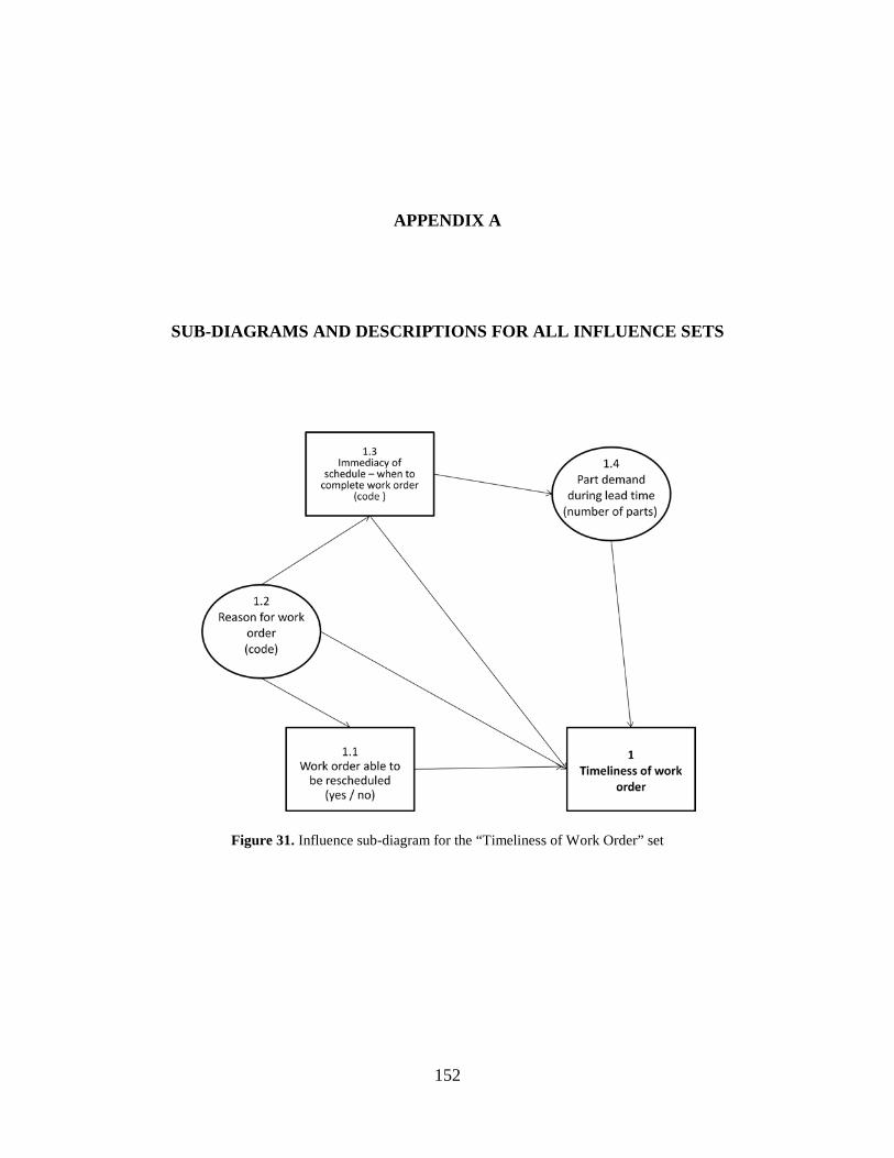
152
APPENDIX A
SUB-DIAGRAMS AND DESCRIPTIONS FOR ALL INFLUENCE SETS
Figure 31. Influence sub-diagram for the “Timeliness of Work Order” set
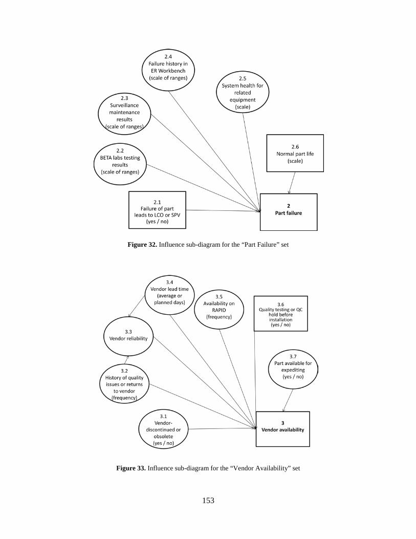
153
Figure 32. Influence sub-diagram for the “Part Failure” set
Figure 33. Influence sub-diagram for the “Vendor Availability” set
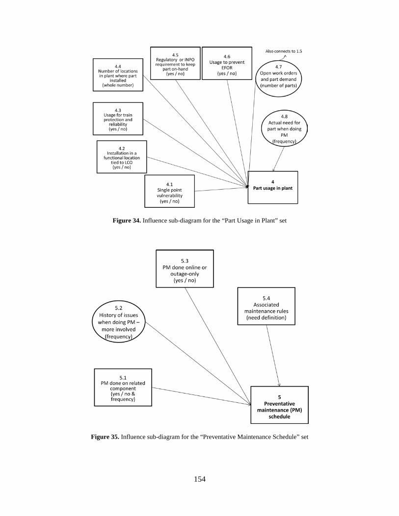
154
Figure 34. Influence sub-diagram for the “Part Usage in Plant” set
Figure 35. Influence sub-diagram for the “Preventative Maintenance Schedule” set

155
Figure 36. Influence sub-diagram for the “Outage Usage” set
Figure 37. Influence sub-diagram for the “Cost Consequences” set

156
Table 22. Description of influences in the “Timeliness of Work Order” set
Number Influence Description 1.1 Work order able to be rescheduled Ability to delay the work to another date
1.2 Reason for work order
Maintenance code for work—elective, corrective, preventative, outage, or other work
1.3 Immediacy of schedule—when to complete work order
Maintenance code for urgency of work—how long able to wait to complete
1.4 Part demand during lead time Parts reserved in inventory for other work
Table 23. Description of influences in the “Part Failure” set
Number Influence Description
2.1 Failure of part leads to LCO or SPV Failure requires plant shut down or derate in 72 hours
2.2 BETA labs testing results Corporate testing of equipment and plant chemicals and their suitability for use
2.3 Surveillance maintenance results Condition of equipment when visually surveyed by maintenance
2.4 Failure history in ER Workbench Recorded previous part failures, kept in system called "ER Workbench"
2.5 System health for related equipment Regulated color-coded scale for condition of equipment in plant
2.6 Normal part life Expected life of installed plant equipment

157
Table 24. Description of influences in the “Vendor Availability” set
Number Influence Description
3.1 Vendor discontinued or obsolete Ability to procure the part as-is, without engineering changes for obsolescence
3.2 History of quality issues or returns to vendor
Record of instances parts were returned to vendor after purchase for substandard quality
3.3 Vendor reliability Ability of vendor to supply quality parts when ordered in a timely manner
3.4 Vendor lead time Elapsed time between part order and receipt from vendor
3.5 Availability on RAPID
Availability of part to borrow or purchase from other nuclear power generation facilities; inventories of participating plants are stored in "RAPID"
3.6 Quality testing or QC hold before installation
Requirement to hold parts after vendor receipt for quality testing
3.7 Part available for expediting Ability of vendor to expedite order and reduce lead time
Table 25. Description of influences in the “Part Usage in Plant” set
Number Influence Description
4.1 Single point vulnerability Installation of part at locations that intersect electricity production trains
4.2 Installation in a functional location tied to LCO
Installation of part at locations that cause derate or shutdown 72 hours after failure
4.3 Usage for train protection and reliability Use of parts to maintain safety on electricity production lines
4.4 Number of locations in plant where part installed
List of plant locations where part is installed
4.5 Regulatory or INPO requirement to keep part on hand
Regulatory need to keep parts on hand in inventory
4.6 Usage to prevent EFOR Use of parts in preventative maintenance to avoid equipment forced outage
4.7 Open work orders and part demand List of all work orders in queue and corresponding demand for part
4.8 Actual need for part when doing PM
Frequency the part is actually used during preventative maintenance work versus requested by plant and later returned to warehouse

158
Table 26. Description of influences in the “Preventative Maintenance Schedule” set
Number Influence Description
5.1 PM done on related component
Need to perform regularly scheduled preventative maintenance on components on which part is installed
5.2 History of issues when doing PM
List of work delays, maintenance scope creep, etc. incurred during previous preventative maintenance
5.3 PM done online or outage only
Ability to complete preventative maintenance work while plant is running or only during outage
5.4 Associated maintenance rules Maintenance requirements for parts and corresponding components
Table 27. Description of influences in the “Outage Usage” set
Number Influence Description
6.1 Scheduled for use during outage List of outage related work orders on which part is requested
6.2 Actual use during outage—no returns
List of outage related work orders on which part is actually used instead of returned to warehouse
6.3 Used outage only vs. online Requirement to install part only when plant is offline for outage
Table 28. Description of influences in the “Cost Consequences” set
Number Influence Description
7.1 Expediting costs Costs to expedite part order from vendor to prevent offlining or derating plant
7.2 Cost of replacement power
Costs associated with generating power from alternate sources or buying power to satisfy consumer demand due to unexpected offlining or derating of nuclear facility

159
APPENDIX B
INTERVIEW INSTRUCTIONS, QUESTIONS, AND JUDGMENTS
B.1 EMPLOYEE INTERVIEW INSTRUCTIONS
During this phone call (15 to 20 minute maximum), you will be presented with a series of
pairwise comparisons and be asked to
1. identify which item is more important with respect to the specific spare parts related issue being studied and
2. determine how much more important that item is over the other item.
Your responses will be aggregated with other employees answering the same questions,
and in no way you will be personally identified in the process. You have been selected to
participate in this process based on your knowledge, experience, and job function. Your
cooperation is greatly appreciated.
The scale for how much more one item is preferred over the other is as follows:
• Equal – no difference between the two items • Moderate • Strong • Very strong

160
As an example of a pairwise comparison, suppose you are buying a car. The issue at
hand is determining which characteristics of the car are most important in the purchase decision.
You might base it on the following items:
• Price, miles per gallon, and car color
Then the pairwise comparisons are to consider each pair of characteristics with respect to
the purchase decision, select which item is more important, and then state how much more
important it is. The three comparisons are
1. Price vs. miles per gallon 2. Price vs. car color 3. Miles per gallon vs. car color
Consider option 1: Price vs. miles per gallon. If the car’s miles per gallon are more
important to you than its price, you would say miles per gallon. Then you will say moderate if
the car’s miles per gallon is slightly more important to you than its overall price.
B.2 PAIRWISE COMPARISON QUESTIONS FOR EACH INFLUENCE SET
Table 29. Pairwise comparisons for the “Timeliness of Work Order” set
# Column A vs. Column B 1 1.1 Work order able to be rescheduled 1.2 Reason for work order
2 1.1 Work order able to be rescheduled 1.3 Immediacy of schedule—when to complete the work order
3 1.1 Work order able to be rescheduled 1.4 Part demand during lead time
4 1.2 Reason for work order 1.3 Immediacy of schedule—when to complete the work order
5 1.2 Reason for work order 1.4 Part demand during lead time
6 1.3 Immediacy of schedule—when to complete the work order 1.4 Part demand during lead time

161
Table 30. Pairwise comparisons for the “Part Failure” set
# Column A vs. Column B
1 2.1 Failure of part leads to LCO or SPV 2.2 BETA labs testing results
2 2.1 Failure of part leads to LCO or SPV 2.3 Surveillance maintenance results
3 2.1 Failure of part leads to LCO or SPV 2.4 Failure history in ER Workbench
4 2.1 Failure of part leads to LCO or SPV 2.5
System health for related equipment
5 2.1 Failure of part leads to LCO or SPV 2.6 Normal part life
6 2.2 BETA labs testing results 2.3 Surveillance maintenance results 7 2.2 BETA labs testing results 2.4 Failure history in ER Workbench
8 2.2 BETA labs testing results 2.5 System health for related equipment
9 2.2 BETA labs testing results 2.6 Normal part life 10 2.3 Surveillance maintenance results 2.4 Failure history in ER Workbench
11 2.3 Surveillance maintenance results 2.5 System health for related equipment
12 2.3 Surveillance maintenance results 2.6 Normal part life
13 2.4 Failure history in ER Workbench 2.5 System health for related equipment
14 2.4 Failure history in ER Workbench 2.6 Normal part life
15 2.5 System health for related equipment 2.6 Normal part life

162
Table 31. Pairwise comparisons for the “Vendor Availability” set
# Column A vs. Column B
1 3.1 Vendor discontinued or obsolete 3.2 History of quality issues or vendor returns
2 3.1 Vendor discontinued or obsolete 3.3 Vendor reliability 3 3.1 Vendor discontinued or obsolete 3.4 Vendor lead time 4 3.1 Vendor discontinued or obsolete 3.5 Availability on RAPID
5 3.1 Vendor discontinued or obsolete 3.6 Quality testing or QC hold before installation
6 3.1 Vendor discontinued or obsolete 3.7 Part available for expediting
7 3.2 History of quality issues or vendor returns 3.3 Vendor reliability
8 3.2 History of quality issues or vendor returns 3.4 Vendor lead time
9 3.2 History of quality issues or vendor returns 3.5 Availability on RAPID
10 3.2 History of quality issues or vendor returns 3.6
Quality testing or QC hold before installation
11 3.2 History of quality issues or vendor returns 3.7 Part available for expediting
12 3.3 Vendor reliability 3.4 Vendor lead time 13 3.3 Vendor reliability 3.5 Availability on RAPID
14 3.3 Vendor reliability 3.6 Quality testing or QC hold before installation
15 3.3 Vendor reliability 3.7 Part available for expediting 16 3.4 Vendor lead time 3.5 Availability on RAPID
17 3.4 Vendor lead time 3.6 Quality testing or QC hold before installation
18 3.4 Vendor lead time 3.7 Part available for expediting
19 3.5 Availability on RAPID 3.6 Quality testing or QC hold before installation
20 3.5 Availability on RAPID 3.7 Part available for expediting
21 3.6 Quality testing or QC hold before installation 3.7 Part available for expediting

163
Table 32. Pairwise comparisons for the “Part Usage in Plant” set
# Column A vs. Column B
1 4.1 Single point vulnerability 4.2 Installation in a functional location tied to LCO
2 4.1 Single point vulnerability 4.3 Usage for equipment train protection and reliability
3 4.1 Single point vulnerability 4.4 Number of locations in plant where part installed
4 4.1 Single point vulnerability 4.5 Regulatory or INPO requirement to keep part on hand
5 4.1 Single point vulnerability 4.6 Usage to prevent EFOR 6 4.1 Single point vulnerability 4.7 Open work orders and part demand
7 4.1 Single point vulnerability 4.8 Actual need for part when doing PM
8 4.2 Installation in a functional location tied to LCO 4.3
Usage for equipment train protection and reliability
9 4.2 Installation in a functional location tied to LCO 4.4
Number of locations in plant where part installed
10 4.2 Installation in a functional location tied to LCO 4.5
Regulatory or INPO requirement to keep part on hand
11 4.2 Installation in a functional location tied to LCO 4.6 Usage to prevent EFOR
12 4.2 Installation in a functional location tied to LCO 4.7 Open work orders and part demand
13 4.2 Installation in a functional location tied to LCO 4.8
Actual need for part when doing PM
14 4.3 Usage for equipment train protection and reliability 4.4
Number of locations in plant where part installed
15 4.3 Usage for equipment train protection and reliability 4.5
Regulatory or INPO requirement to keep part on hand
16 4.3 Usage for equipment train protection and reliability 4.6 Usage to prevent EFOR
17 4.3 Usage for equipment train protection and reliability 4.7 Open work orders and part demand
18 4.3 Usage for equipment train protection and reliability 4.8
Actual need for part when doing PM
19 4.4 Number of locations in plant where part installed 4.5
Regulatory or INPO requirement to keep part on hand
20 4.4 Number of locations in plant where part installed 4.6 Usage to prevent EFOR

164
Table 32 (continued).
#
Column A vs.
Column B
21 4.4 Number of locations in plant where part installed 4.7 Open work orders and part demand
22 4.4 Number of locations in plant where part installed 4.8
Actual need for part when doing PM
23 4.5 Regulatory or INPO requirement to keep part on hand 4.6 Usage to prevent EFOR
24 4.5 Regulatory or INPO requirement to keep part on hand 4.7 Open work orders and part demand
25 4.5 Regulatory or INPO requirement to keep part on hand 4.8
Actual need for part when doing PM
26 4.6 Usage to prevent EFOR 4.7 Open work orders and part demand
27 4.6 Usage to prevent EFOR 4.8 Actual need for part when doing PM
28 4.7 Open work orders and part demand 4.8 Actual need for part when doing PM
Table 33. Pairwise comparisons for the “Preventative Maintenance Schedule” set
# Column A vs. Column B
1 5.1 PM done on related component 5.2 History of issues when doing PM–more involved
2 5.1 PM done on related component 5.3 PM done online or outage only
3 5.1 PM done on related component 5.4 Associated maintenance rules
4 5.2 History of issues when doing PM– more involved 5.3 PM done online or outage only
5 5.2 History of issues when doing PM– more involved 5.4 Associated maintenance rules
6 5.3 PM done online or outage only 5.4 Associated maintenance rules

165
Table 34. Pairwise comparisons for the “Outage Usage” set
# Column A vs. Column B
1 6.1 Scheduled for usage in outage—no returns 6.2 Actual usage in outage—no returns
2 6.1 Scheduled for usage in outage—no returns 6.3 Used outage only vs. online
3 6.2 Actual usage in outage—no returns 6.3 Used outage only vs. online
Table 35. Pairwise comparisons for the “Cost Consequences” set
# Column A vs. Column B 1 7.1 Expediting costs 7.2 Cost of replacement power
Table 36. Pairwise comparisons for the set of overall influences
# Column A vs. Column B 1 0.1 Timeliness of work order 0.2 Part failure 2 0.1 Timeliness of work order 0.3 Vendor availability 3 0.1 Timeliness of work order 0.4 Part usage in plant 4 0.1 Timeliness of work order 0.5 Preventative maintenance schedule 5 0.1 Timeliness of work order 0.6 Outage usage 6 0.1 Timeliness of work order 0.7 Cost consequences 7 0.2 Part failure 0.3 Vendor availability 8 0.2 Part failure 0.4 Part usage in plant 9 0.2 Part failure 0.5 Preventative maintenance schedule 10 0.2 Part failure 0.6 Outage usage 11 0.2 Part failure 0.7 Cost consequences 12 0.3 Vendor availability 0.4 Part usage in plant 13 0.3 Vendor availability 0.5 Preventative maintenance schedule 14 0.3 Vendor availability 0.6 Outage usage 15 0.3 Vendor availability 0.7 Cost consequences 16 0.4 Part usage in plant 0.5 Preventative maintenance schedule 17 0.4 Part usage in plant 0.6 Outage usage 18 0.4 Part usage in plant 0.7 Cost consequences 19 0.5 Preventative maintenance schedule 0.6 Outage usage 20 0.5 Preventative maintenance schedule 0.7 Cost consequences 21 0.6 Outage usage 0.7 Cost consequences

166
B.3 REVISED SUBSET JUDGMENTS
Table 37. Revised judgments for all respondents in the “Part Failure” set
Judgments – Employees 10, 9, 11, 13, 12 2.1 2.2 2.3 2.4 2.5 2.6
Judgments
2.1 1 5, 7, 7 5,
7 3, 1, 5, 3,
3 5, 5, 5, 1, 3 3, 1, 5, 1/3,
1/5 5, 5, 3, 1, 1/3
2.2 1 1/3, 1/5, 1,
1, 1 3, 1/3, 1, 1/3,
3 3, 1/5, 1, 1/3,
5 5, 1/3, 1, 1/3,
3 2.3 1 3, 5, 3, 1/5, 1 3, 3, 3, 1/5, 1 5, 5, 3, 1/5, 1 2.4 1 1, 1/3, 1, 1, 5 3, 3, 1, 3, 1 2.5 1 3, 5, 1/3, 3, 1 2.6 1
Table 38. Revised judgments for all respondents in the “Vendor Availability” set
Judgments – Employees 3, 5, 1, 4, 2 3.1 3.2 3.3 3.4 3.5 3.6 3.7
Judgments
3.1 1
1/5, 7, 7, 1/5,
7 1/7, 7, 7,
5, 5 1/3, 7, 7,
7, 3 1/5, 7, 3, 1/7, 1/7
1/3, 7, 7, 7, 7
1/3, 7, 7, 7, 5
3.2 1 1, 1, 1, 7,
1/3 5, 1, 1/5,
7, 1/3 1, 1/3, 1/3,
7, 1/3 5, 1, 1, 1/7, 5
5, 1/3, 1/5, 5, 1/5
3.3 1 7, 1/3, 1/5,
5, 3 5, 1/7, 1/5,
5, 3 5, 3, 1, 1/5, 7
5, 1/3, 1/5, 5, 5
3.4 1 1, 1/7, 5, 3,
3 1, 1, 5, 1/5, 3 3, 1, 1, 1, 3
3.5 1 1, 7, 5, 1/3, 1/3
1, 7, 1, 1/3, 1/3
3.6 1 1, 1/3, 1/7,
5, 1/3 3.7 1
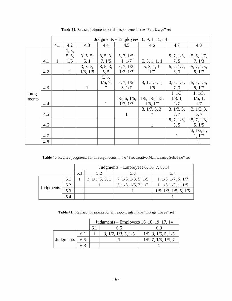
167
Table 39. Revised judgments for all respondents in the “Part Usage” set
Judgments – Employees 10, 9, 1, 15, 14 4.1 4.2 4.3 4.4 4.5 4.6 4.7 4.8
Judg-ments
4.1 1
1, 5, 5, 5, 1/5
3, 5, 5, 5, 1
3, 5, 3, 7, 1/5
5, 7, 1/5, 1, 1/7 5, 5, 1, 1, 1
5, 7, 1/3, 7, 5
5, 5, 1/7, 7, 1/3
4.2 1 3, 3, 7, 1/3, 1/5
3, 5, 3, 5, 5
5, 7, 1/3, 1/3, 1/7
5, 3, 1, 1, 1/7
5, 7, 1/7, 3, 3
5, 7, 1/5, 5, 1/7
4.3 1
5, 5, 1/5, 7,
7 5, 7, 1/5,
3, 1/7 3, 1, 1/5, 1,
1/5 3, 5, 1/5,
7, 3 5, 5, 1/5,
5, 1/7
4.4 1 1/5, 5, 1/5,
1/7, 1/7 1/5, 1/5, 1/5,
1/5, 1/7
1, 1/3, 1/3, 1,
1/7
1, 1/5, 1/5, 1,
1/7
4.5 1 3, 1/7, 3, 3,
7 3, 1/3, 3,
5, 7 3, 1/3, 3,
5, 7
4.6 1 5, 7, 1/3,
5, 5 5, 7, 1/3,
5, 1/5
4.7 1 3, 1/3, 1,
1, 1/7 4.8 1
Table 40. Revised judgments for all respondents in the “Preventative Maintenance Schedule” set
Judgments – Employees 6, 16, 7, 8, 14 5.1 5.2 5.3 5.4
Judgments
5.1 1 3, 1/3, 5, 5, 1 7, 1/5, 1/3, 5, 1/5 1, 1/5, 1/7, 5, 1/7 5.2 1 3, 1/3, 1/5, 3, 1/3 1, 1/5, 1/3, 1, 1/5 5.3 1 1/5, 1/3, 1/5, 5, 1/5 5.4 1
Table 41. Revised judgments for all respondents in the “Outage Usage” set
Judgments – Employees 16, 18, 19, 17, 14 6.1 6.5 6.3
Judgments 6.1 1 3, 1/7, 1/3, 5, 1/5 1/5, 3, 1/5, 5, 1/5 6.5 1 1/5, 7, 1/5, 1/5, 7 6.3 1
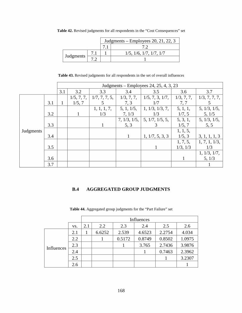
168
Table 42. Revised judgments for all respondents in the “Cost Consequences” set
Judgments – Employees 20, 21, 22, 3 7.1 7.2
Judgments 7.1 1 1/5, 1/6, 1/7, 1/7, 1/7 7.2 1
Table 43. Revised judgments for all respondents in the set of overall influences
Judgments – Employees 24, 25, 4, 3, 23 3.1 3.2 3.3 3.4 3.5 3.6 3.7
Judgments
3.1 1 1/5, 7, 7,
1/5, 7 1/7, 7, 7, 5,
5 1/3, 7, 7,
7, 3 1/5, 7, 3, 1/7,
1/7 1/3, 7, 7,
7, 7 1/3, 7, 7, 7,
5
3.2 1 1, 1, 1, 7,
1/3 5, 1, 1/5,
7, 1/3 1, 1/3, 1/3, 7,
1/3 5, 1, 1, 1/7, 5
5, 1/3, 1/5, 5, 1/5
3.3 1 7, 1/3, 1/5,
5, 3 5, 1/7, 1/5, 5,
3 5, 3, 1, 1/5, 7
5, 1/3, 1/5, 5, 5
3.4 1 1, 1/7, 5, 3, 3 1, 1, 5, 1/5, 3 3, 1, 1, 1, 3
3.5 1 1, 7, 5, 1/3, 1/3
1, 7, 1, 1/3, 1/3
3.6 1 1, 1/3, 1/7,
5, 1/3 3.7 1
B.4 AGGREGATED GROUP JUDGMENTS
Table 44. Aggregated group judgments for the “Part Failure” set
Influences vs. 2.1 2.2 2.3 2.4 2.5 2.6
Influences
2.1 1 6.6252 2.539 4.6523 2.2754 4.034 2.2 1 0.5172 0.8749 0.8502 1.0975 2.3 1 3.765 2.7436 3.9876 2.4 1 0.7463 2.3962 2.5 1 3.2307 2.6 1

169
Table 45. Aggregated group judgments for the “Vendor Availability” set
Influences vs. 3.1 3.2 3.3 3.4 3.5 3.6 3.7
Influences
3.1 1 5.9131 5.8448 5.7842 4.089 6.0039 5.8941 3.2 1 1.0259 1.3342 0.5024 1.8084 1.0237 3.3 1 1.4763 1.0968 2.7659 1.2873 3.4 1 2.2147 2.5485 1.4087 3.5 1 4.9444 3.4975 3.6 1 0.4127 3.7 1
Table 46. Aggregated group judgments for the “Part Usage in Plant” set
Influences vs. 4.1 4.2 4.3 4.4 4.5 4.6 4.7 4.8
Influences
4.1 1 3.7368 4.0862 4.7912 3.0162 2.5849 6.4246 5.0167 4.2 1 1.3807 4.7875 2.7329 1.8494 4.3705 4.717 4.3 1 6.1929 3.8666 1.0654 5.2791 4.1328 4.4 1 1.5678 0.1899 0.6526 0.6134 4.5 1 2.871 3.7771 3.7771 4.6 1 5.5742 4.7274 4.7 1 0.8623 4.8 1
Table 47. Aggregated judgments for the “Preventative Maintenance Schedule” set
Influences vs. 5.1 5.2 5.3 5.4
Influences
5.1 1 3.348 6.2656 1.3212 5.2 1 2.774 0.9458 5.3 1 0.6685 5.4 1
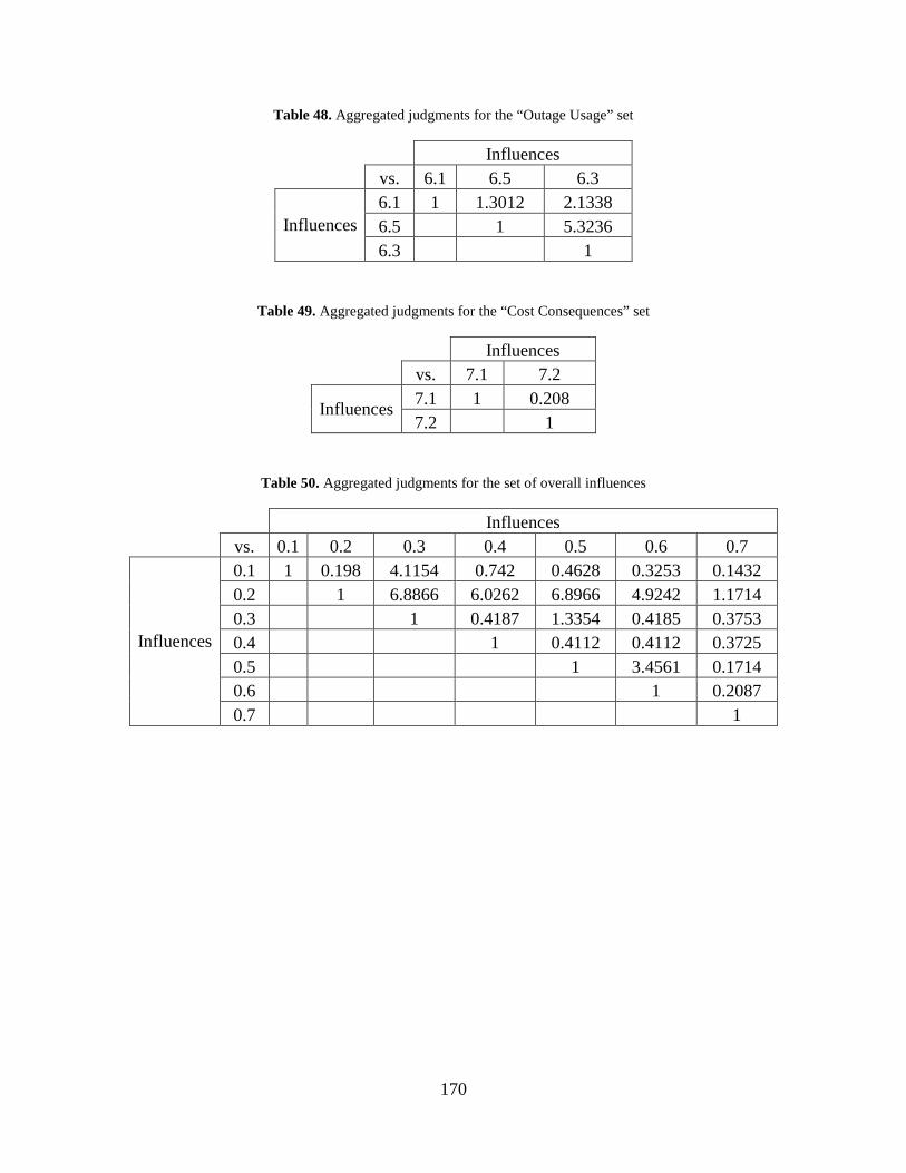
170
Table 48. Aggregated judgments for the “Outage Usage” set
Influences vs. 6.1 6.5 6.3
Influences 6.1 1 1.3012 2.1338 6.5 1 5.3236 6.3 1
Table 49. Aggregated judgments for the “Cost Consequences” set
Influences vs. 7.1 7.2
Influences 7.1 1 0.208 7.2 1
Table 50. Aggregated judgments for the set of overall influences
Influences vs. 0.1 0.2 0.3 0.4 0.5 0.6 0.7
Influences
0.1 1 0.198 4.1154 0.742 0.4628 0.3253 0.1432 0.2 1 6.8866 6.0262 6.8966 4.9242 1.1714 0.3 1 0.4187 1.3354 0.4185 0.3753 0.4 1 0.4112 0.4112 0.3725 0.5 1 3.4561 0.1714 0.6 1 0.2087 0.7 1

171
APPENDIX C
HISTORICAL SIMULATION CODE AND RESULTS
C.1 HISTORICAL SIMULATION CODE—UNDERESTIMATE DEMAND
The following script for the historical numerical simulation where average demand per plant
request is underestimated was written in MATLAB. The highlighted section is modified to both
overestimate demand and find an intermediate demand estimate; modifications are shown in
Appendices C.2 and C.3, respectively.
% Inventory Policy Analysis % Base Stock Version % Part data file and LCO data file - stock codes have to be numerical order clear clc % Open file to write regression inputs fname2 = input('Name of output data file ', 's'); fid3 = fopen(fname2, 'wt'); fprintf(fid3, 'Col1: Base stock percent b \n'); fprintf(fid3, 'Col2: missed days not @ LCO, Col3: missed days @ LCO \n'); fprintf(fid3, 'Col4: total part capital costs \n\n'); % Open file to write starting inventory values fname4 = input('Name of starting inventory output file ', 's'); fid4 = fopen(fname4, 'wt'); fprintf(fid4, 'Col1: b, Col2: Part number, Col3: Calculated base stock \n'); fprintf(fid4, 'Col4: Part cost, Col5: Base stock investment \n\n');
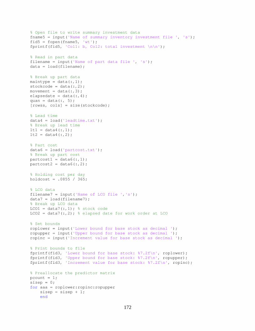
172
% Open file to write summary investment data fname5 = input('Name of summary inventory investment file ', 's'); fid5 = fopen(fname5, 'wt'); fprintf(fid5, 'Col1: b, Col2: total investment \n\n'); % Read in part data filename = input('Name of part data file ', 's'); data = load(filename); % Break up part data maintype = data(:,1); stockcode = data(:,2); movement = data(:,3); elapsedate = data(:,4); quan = data(:, 5); [rowss, cols] = size(stockcode); % Lead time data4 = load('leadtime.txt'); % Break up lead time lt1 = data4(:,1); lt2 = data4(:,2); % Part cost data6 = load('partcost.txt'); % Break up part cost partcost1 = data6(:,1); partcost2 = data6(:,2); % Holding cost per day holdcost = .0855 / 365; % LCO data filename7 = input('Name of LCO file ','s'); data7 = load(filename7); % Break up LCO data LCO1 = data7(:,1); % stock code LCO2 = data7(:,2); % elapsed date for work order at LCO % Set bounds roplower = input('Lower bound for base stock as decimal '); ropupper = input('Upper bound for base stock as decimal '); ropinc = input('Increment value for base stock as decimal '); % Print bounds to file fprintf(fid3, 'Lower bound for base stock: %7.2f\n', roplower); fprintf(fid3, 'Upper bound for base stock: %7.2f\n', ropupper); fprintf(fid3, 'Increment value for base stock: %7.2f\n', ropinc); % Preallocate the predictor matrix pcount = 1; sizep = 0; for aaa = roplower:ropinc:ropupper sizep = sizep + 1; end
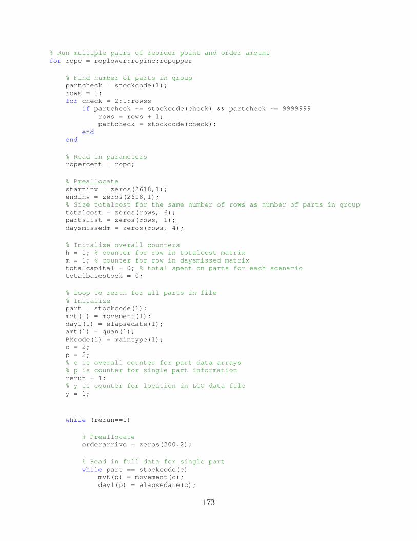
173
% Run multiple pairs of reorder point and order amount for ropc = roplower:ropinc:ropupper % Find number of parts in group partcheck = stockcode(1); rows = 1; for check = 2:1:rowss if partcheck ~= stockcode(check) && partcheck ~= 9999999 rows = rows + 1; partcheck = stockcode(check); end end % Read in parameters ropercent = ropc; % Preallocate startinv = zeros(2618,1); endinv = zeros(2618,1); % Size totalcost for the same number of rows as number of parts in group totalcost = zeros(rows, 6); partslist = zeros(rows, 1); daysmissedm = zeros(rows, 4); % Initalize overall counters h = 1; % counter for row in totalcost matrix m = 1; % counter for row in daysmissed matrix totalcapital = 0; % total spent on parts for each scenario totalbasestock = 0; % Loop to rerun for all parts in file % Initalize part = stockcode(1); mvt(1) = movement(1); day1(1) = elapsedate(1); amt(1) = quan(1); PMcode(1) = maintype(1); c = 2; p = 2; % c is overall counter for part data arrays % p is counter for single part information rerun = 1; % y is counter for location in LCO data file y = 1; while (rerun==1) % Preallocate orderarrive = zeros(200,2); % Read in full data for single part while part == stockcode(c) mvt(p) = movement(c); day1(p) = elapsedate(c);
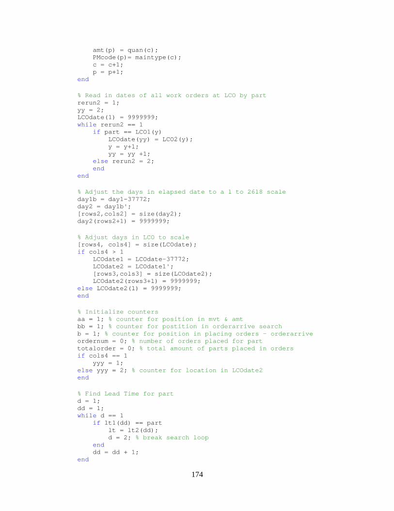
174
amt(p) = quan(c); PMcode(p)= maintype(c); c = c+1; p = p+1; end % Read in dates of all work orders at LCO by part rerun2 = 1; yy = 2; LCOdate(1) = 9999999; while rerun2 == 1 if part == LCO1(y) LCOdate(yy) = LCO2(y); y = y+1; yy = yy +1; else rerun2 = 2; end end % Adjust the days in elapsed date to a 1 to 2618 scale day1b = day1-37772; day2 = day1b'; [rows2,cols2] = size(day2); day2(rows2+1) = 9999999; % Adjust days in LCO to scale [rows4, cols4] = size(LCOdate); if cols4 > 1 LCOdate1 = LCOdate-37772; LCOdate2 = LCOdate1'; [rows3,cols3] = size(LCOdate2); LCOdate2(rows3+1) = 9999999; else LCOdate2(1) = 9999999; end % Initialize counters aa = 1; % counter for position in mvt & amt bb = 1; % counter for postition in orderarrive search b = 1; % counter for position in placing orders - orderarrive ordernum = 0; % number of orders placed for part totalorder = 0; % total amount of parts placed in orders if cols4 == 1 yyy = 1; else yyy = 2; % counter for location in LCOdate2 end % Find Lead Time for part d = 1; dd = 1; while d == 1 if lt1(dd) == part lt = lt2(dd); d = 2; % break search loop end dd = dd + 1; end

175
% Find part cost for part g = 1; gg = 1; while g == 1 if partcost1(gg) == part partcost = partcost2(gg); g = 2; % break search loop end gg = gg + 1; end % Initialize total cost info matrix partslist(h) = part; totalcost(h,2) = partcost; % Initialize orderarrive % Writes over this value but has something to compare to before first % order placed orderarrive(1,1) = 9999999; orderarrrive(1,2) = 9999999; % For loop to calculate inventory status each day and ordering
% Start at June 1, 2003 (day 37773), end at July 31, 2010 (day % 40390),
% using Excel elapsed time for days for i=1:1:2618 % Set day's starting inventory if i == 1 [mvtrows, mvtcols] = size(mvt); mvtcount = 0; demandcounter = 0; for t = 1:1:mvtcols if mvt(t) == 261 mvtcount = mvtcount + amt(t); demandcounter = demandcounter + 1; else mvtcount = mvtcount - amt(t); %Calculate total used demands for that partover all days end end % Base stock - multiple of average demand size % Take ceiling for whole number avgdemand = mvtcount/demandcounter; reorder = ceil(ropercent * avgdemand); startinv(i) = reorder; % force in base stock IP fprintf(fid4, '%7.2f', ropercent); fprintf(fid4, ' %12.2f', part); fprintf(fid4, ' %12.2f', reorder); fprintf(fid4, ' %12.2f', partcost); basestockcost = reorder * partcost; totalbasestock = totalbasestock + basestockcost; fprintf(fid4, ' %12.2f\n', basestockcost);
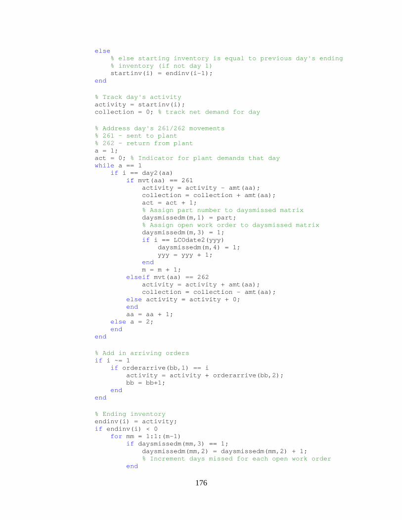
176
else % else starting inventory is equal to previous day's ending % inventory (if not day 1) startinv(i) = endinv(i-1); end % Track day's activity activity = startinv(i); collection = 0; % track net demand for day % Address day's 261/262 movements % 261 - sent to plant % 262 - return from plant a = 1; act = 0; % Indicator for plant demands that day while a == 1 if i == day2(aa) if mvt(aa) == 261 activity = activity - amt(aa); collection = collection + amt(aa); act = act + 1; % Assign part number to daysmissed matrix daysmissedm(m,1) = part; % Assign open work order to daysmissed matrix daysmissedm(m,3) = 1; if i == LCOdate2(yyy) daysmissedm(m,4) = 1; yyy = yyy + 1; end m = m + 1; elseif mvt(aa) == 262 activity = activity + amt(aa); collection = collection - amt(aa); else activity = activity + 0; end aa = aa + 1; else a = 2; end end % Add in arriving orders if i ~= 1 if orderarrive(bb,1) == i activity = activity + orderarrive(bb,2); bb = bb+1; end end % Ending inventory endinv(i) = activity; if endinv(i) < 0 for mm = 1:1:(m-1) if daysmissedm(mm,3) == 1; daysmissedm(mm,2) = daysmissedm(mm,2) + 1; % Increment days missed for each open work order end
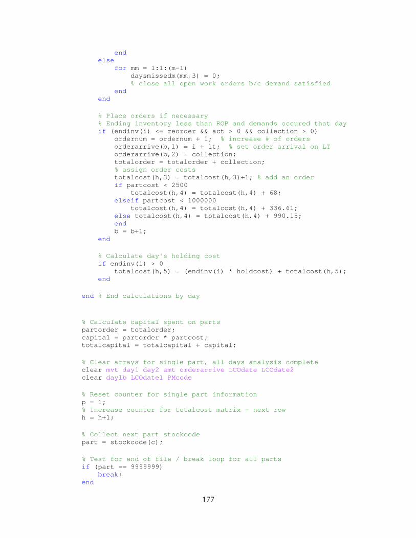
177
end else for mm = 1:1:(m-1) daysmissedm(mm,3) = 0; % close all open work orders b/c demand satisfied end end % Place orders if necessary % Ending inventory less than ROP and demands occured that day if (endinv(i) <= reorder && act > 0 && collection > 0) ordernum = ordernum + 1; % increase # of orders orderarrive(b,1) = i + lt; % set order arrival on LT orderarrive(b,2) = collection; totalorder = totalorder + collection; % assign order costs totalcost(h,3) = totalcost(h,3)+1; % add an order if partcost < 2500 totalcost(h,4) = totalcost(h,4) + 68; elseif partcost < 1000000 totalcost(h,4) = totalcost(h,4) + 336.61; else totalcost(h,4) = totalcost(h,4) + 990.15; end b = b+1; end % Calculate day's holding cost if endinv(i) > 0 totalcost(h,5) = (endinv(i) * holdcost) + totalcost(h,5); end end % End calculations by day % Calculate capital spent on parts partorder = totalorder; capital = partorder * partcost; totalcapital = totalcapital + capital; % Clear arrays for single part, all days analysis complete clear mvt day1 day2 amt orderarrive LCOdate LCOdate2 clear day1b LCOdate1 PMcode % Reset counter for single part information p = 1; % Increase counter for totalcost matrix - next row h = h+1; % Collect next part stockcode part = stockcode(c); % Test for end of file / break loop for all parts if (part == 9999999) break; end
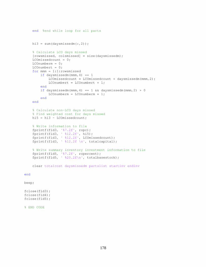
178
end %end while loop for all parts hi3 = sum(daysmissedm(:,2)); % Calculate LCO days missed [rowsmissed, colsmissed] = size(daysmissedm); LCOmissedcount = 0; LCOnumberm = 0; LCOnumbert = 0; for mmm = 1:1:rowsmissed if daysmissedm(mmm,4) == 1 LCOmissedcount = LCOmissedcount + daysmissedm(mmm,2); LCOnumbert = LCOnumbert + 1; end if daysmissedm(mmm,4) == 1 && daysmissedm(mmm,2) > 0 LCOnumberm = LCOnumberm + 1; end end % Calculate non-LCO days missed % Find weighted cost for days missed hi5 = hi3 - LCOmissedcount; % Write information to file fprintf(fid3, '%7.2f', ropc); fprintf(fid3, ' %12.2f', hi5); fprintf(fid3, ' %12.2f', LCOmissedcount); fprintf(fid3, ' %12.2f \n', totalcapital); % Write summary inventory investment information to file fprintf(fid5, '%7.2f', ropercent); fprintf(fid5, ' %20.2f\n', totalbasestock); clear totalcost daysmissedm partslist startinv endinv end beep; fclose(fid3); fclose(fid4); fclose(fid5); % END CODE
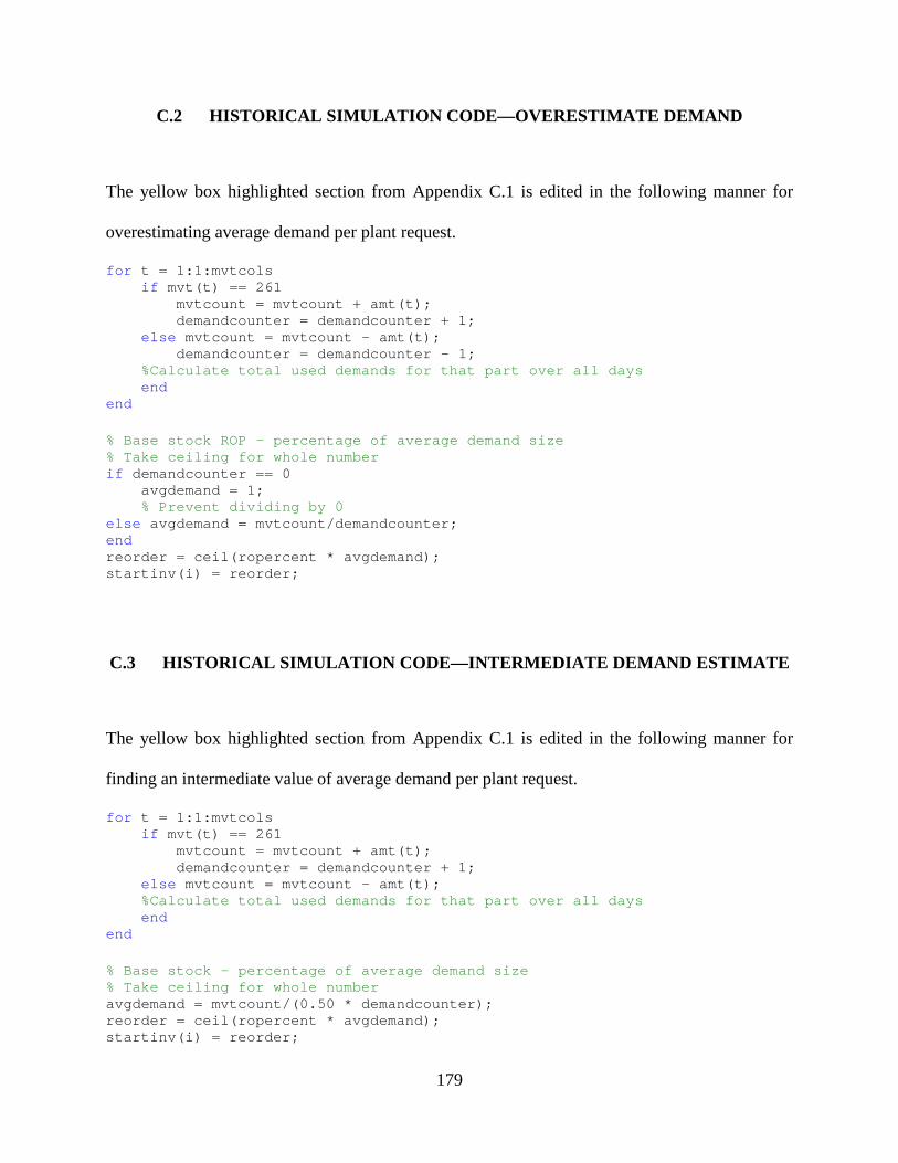
179
C.2 HISTORICAL SIMULATION CODE—OVERESTIMATE DEMAND
The yellow box highlighted section from Appendix C.1 is edited in the following manner for
overestimating average demand per plant request.
for t = 1:1:mvtcols if mvt(t) == 261 mvtcount = mvtcount + amt(t); demandcounter = demandcounter + 1; else mvtcount = mvtcount - amt(t); demandcounter = demandcounter - 1; %Calculate total used demands for that part over all days end end % Base stock ROP - percentage of average demand size % Take ceiling for whole number if demandcounter == 0 avgdemand = 1; % Prevent dividing by 0 else avgdemand = mvtcount/demandcounter; end reorder = ceil(ropercent * avgdemand); startinv(i) = reorder;
C.3 HISTORICAL SIMULATION CODE—INTERMEDIATE DEMAND ESTIMATE
The yellow box highlighted section from Appendix C.1 is edited in the following manner for
finding an intermediate value of average demand per plant request.
for t = 1:1:mvtcols if mvt(t) == 261 mvtcount = mvtcount + amt(t); demandcounter = demandcounter + 1; else mvtcount = mvtcount - amt(t); %Calculate total used demands for that part over all days end end % Base stock - percentage of average demand size % Take ceiling for whole number avgdemand = mvtcount/(0.50 * demandcounter); reorder = ceil(ropercent * avgdemand); startinv(i) = reorder;
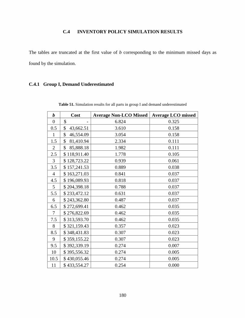
180
C.4 INVENTORY POLICY SIMULATION RESULTS
The tables are truncated at the first value of b corresponding to the minimum missed days as
found by the simulation.
C.4.1 Group I, Demand Underestimated
Table 51. Simulation results for all parts in group I and demand underestimated
b Cost Average Non-LCO Missed Average LCO missed 0 $ - 6.824 0.325
0.5 $ 43,662.51 3.610 0.158 1 $ 46,554.09 3.054 0.158
1.5 $ 81,410.94 2.334 0.111 2 $ 85,888.18 1.982 0.111
2.5 $ 118,911.40 1.778 0.105 3 $ 128,723.22 0.939 0.061
3.5 $ 157,241.53 0.889 0.038 4 $ 163,271.03 0.841 0.037
4.5 $ 196,089.93 0.818 0.037 5 $ 204,398.18 0.788 0.037
5.5 $ 233,472.12 0.631 0.037 6 $ 243,362.80 0.487 0.037
6.5 $ 272,699.41 0.462 0.035 7 $ 276,822.69 0.462 0.035
7.5 $ 313,593.70 0.462 0.035 8 $ 321,159.43 0.357 0.023
8.5 $ 348,431.83 0.307 0.023 9 $ 359,155.22 0.307 0.023
9.5 $ 392,339.19 0.274 0.007 10 $ 395,556.32 0.274 0.005
10.5 $ 430,055.46 0.274 0.005 11 $ 433,554.27 0.254 0.000
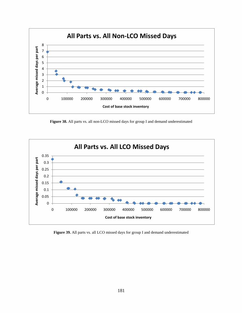
181
Figure 38. All parts vs. all non-LCO missed days for group I and demand underestimated
Figure 39. All parts vs. all LCO missed days for group I and demand underestimated
0
1
2
3
4
5
6
7
8
0 100000 200000 300000 400000 500000 600000 700000 800000
Ave
rage
mis
sed
days
per
par
t
Cost of base stock inventory
All Parts vs. All Non-LCO Missed Days
0
0.05
0.1
0.15
0.2
0.25
0.3
0.35
0 100000 200000 300000 400000 500000 600000 700000 800000
Ave
rage
mis
sed
days
per
par
t
Cost of base stock inventory
All Parts vs. All LCO Missed Days
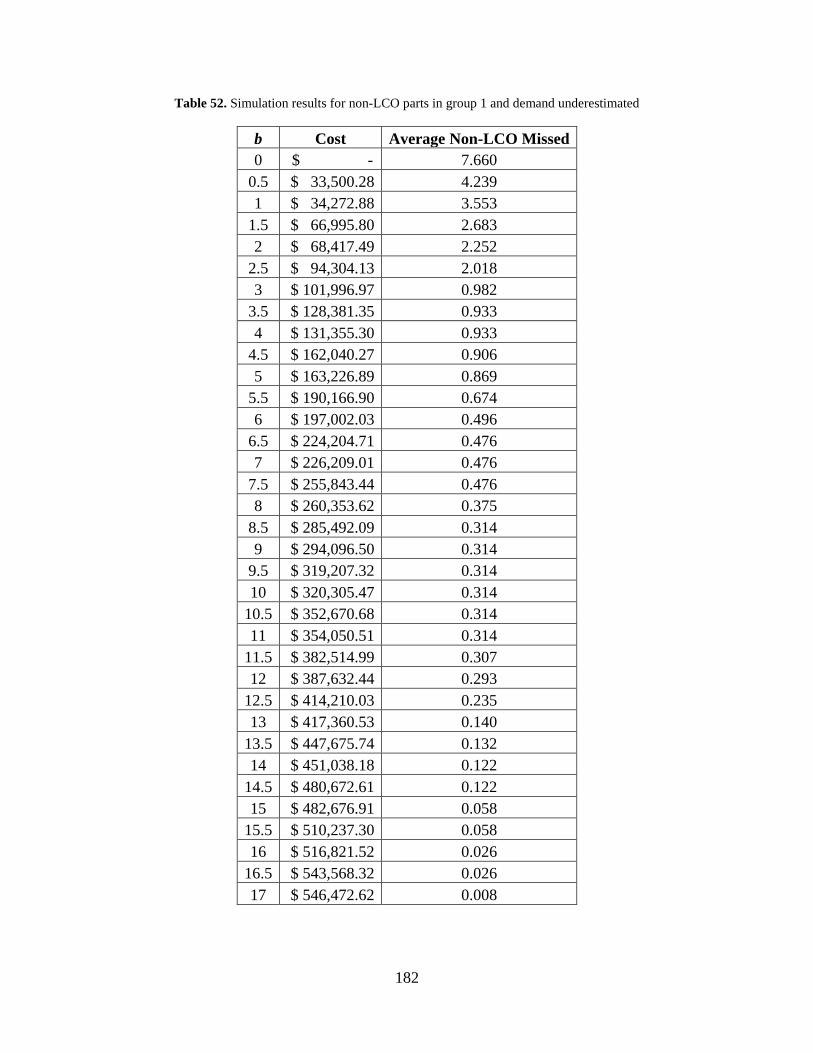
182
Table 52. Simulation results for non-LCO parts in group 1 and demand underestimated
b Cost Average Non-LCO Missed 0 $ - 7.660
0.5 $ 33,500.28 4.239 1 $ 34,272.88 3.553
1.5 $ 66,995.80 2.683 2 $ 68,417.49 2.252
2.5 $ 94,304.13 2.018 3 $ 101,996.97 0.982
3.5 $ 128,381.35 0.933 4 $ 131,355.30 0.933
4.5 $ 162,040.27 0.906 5 $ 163,226.89 0.869
5.5 $ 190,166.90 0.674 6 $ 197,002.03 0.496
6.5 $ 224,204.71 0.476 7 $ 226,209.01 0.476
7.5 $ 255,843.44 0.476 8 $ 260,353.62 0.375
8.5 $ 285,492.09 0.314 9 $ 294,096.50 0.314
9.5 $ 319,207.32 0.314 10 $ 320,305.47 0.314
10.5 $ 352,670.68 0.314 11 $ 354,050.51 0.314
11.5 $ 382,514.99 0.307 12 $ 387,632.44 0.293
12.5 $ 414,210.03 0.235 13 $ 417,360.53 0.140
13.5 $ 447,675.74 0.132 14 $ 451,038.18 0.122
14.5 $ 480,672.61 0.122 15 $ 482,676.91 0.058
15.5 $ 510,237.30 0.058 16 $ 516,821.52 0.026
16.5 $ 543,568.32 0.026 17 $ 546,472.62 0.008
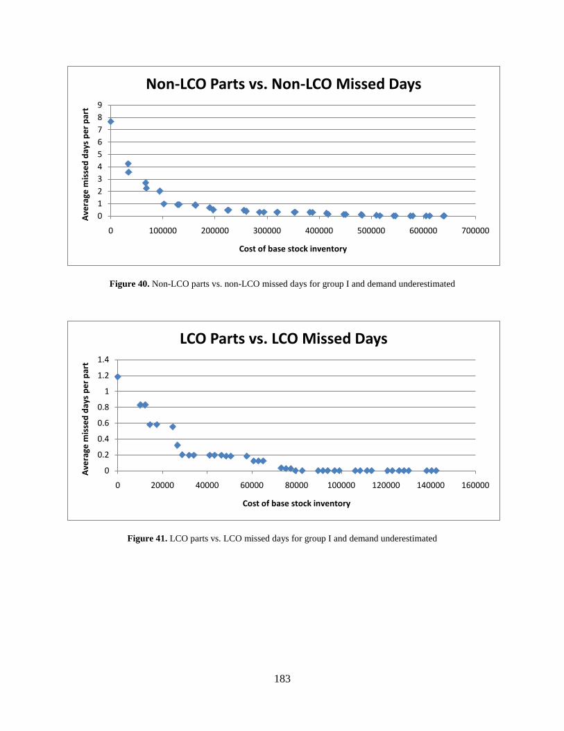
183
Figure 40. Non-LCO parts vs. non-LCO missed days for group I and demand underestimated
Figure 41. LCO parts vs. LCO missed days for group I and demand underestimated
0123456789
0 100000 200000 300000 400000 500000 600000 700000
Ave
rage
mis
sed
days
per
par
t
Cost of base stock inventory
Non-LCO Parts vs. Non-LCO Missed Days
0
0.2
0.4
0.6
0.8
1
1.2
1.4
0 20000 40000 60000 80000 100000 120000 140000 160000
Ave
rage
mis
sed
days
per
par
t
Cost of base stock inventory
LCO Parts vs. LCO Missed Days
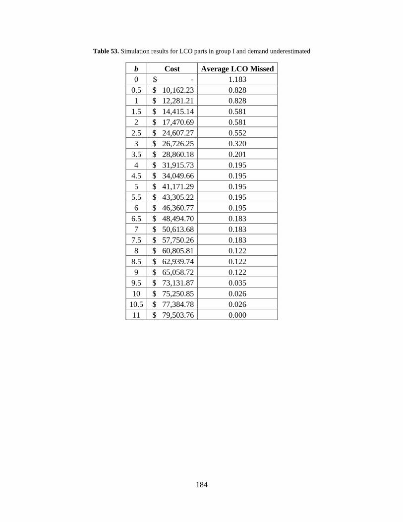
184
Table 53. Simulation results for LCO parts in group I and demand underestimated
b Cost Average LCO Missed 0 $ - 1.183
0.5 $ 10,162.23 0.828 1 $ 12,281.21 0.828
1.5 $ 14,415.14 0.581 2 $ 17,470.69 0.581
2.5 $ 24,607.27 0.552 3 $ 26,726.25 0.320
3.5 $ 28,860.18 0.201 4 $ 31,915.73 0.195
4.5 $ 34,049.66 0.195 5 $ 41,171.29 0.195
5.5 $ 43,305.22 0.195 6 $ 46,360.77 0.195
6.5 $ 48,494.70 0.183 7 $ 50,613.68 0.183
7.5 $ 57,750.26 0.183 8 $ 60,805.81 0.122
8.5 $ 62,939.74 0.122 9 $ 65,058.72 0.122
9.5 $ 73,131.87 0.035 10 $ 75,250.85 0.026
10.5 $ 77,384.78 0.026 11 $ 79,503.76 0.000
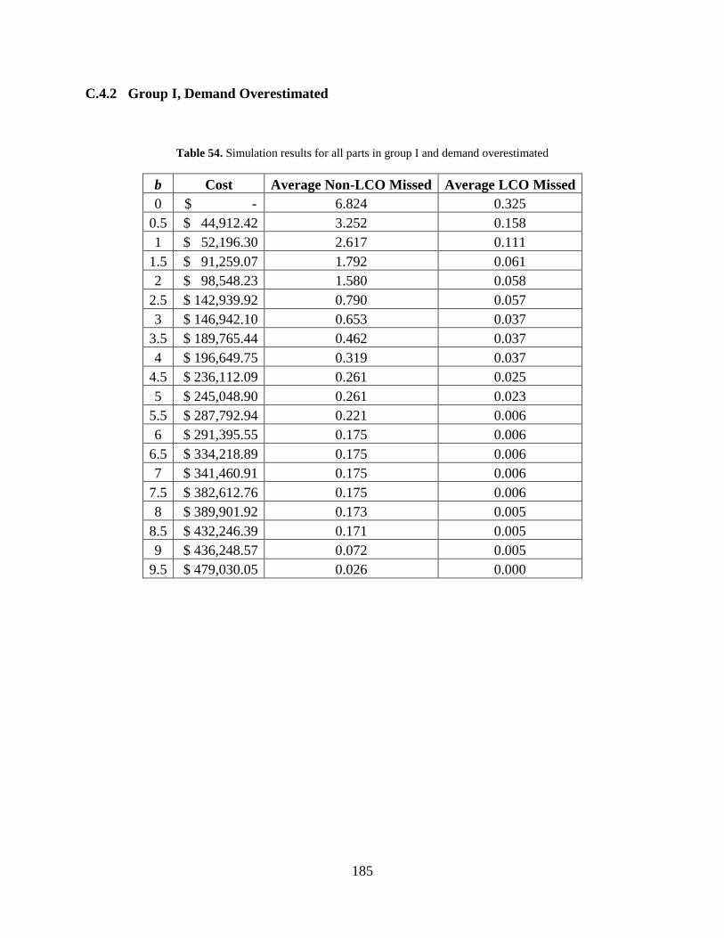
185
C.4.2 Group I, Demand Overestimated
Table 54. Simulation results for all parts in group I and demand overestimated
b Cost Average Non-LCO Missed Average LCO Missed 0 $ - 6.824 0.325
0.5 $ 44,912.42 3.252 0.158 1 $ 52,196.30 2.617 0.111
1.5 $ 91,259.07 1.792 0.061 2 $ 98,548.23 1.580 0.058
2.5 $ 142,939.92 0.790 0.057 3 $ 146,942.10 0.653 0.037
3.5 $ 189,765.44 0.462 0.037 4 $ 196,649.75 0.319 0.037
4.5 $ 236,112.09 0.261 0.025 5 $ 245,048.90 0.261 0.023
5.5 $ 287,792.94 0.221 0.006 6 $ 291,395.55 0.175 0.006
6.5 $ 334,218.89 0.175 0.006 7 $ 341,460.91 0.175 0.006
7.5 $ 382,612.76 0.175 0.006 8 $ 389,901.92 0.173 0.005
8.5 $ 432,246.39 0.171 0.005 9 $ 436,248.57 0.072 0.005
9.5 $ 479,030.05 0.026 0.000

186
Figure 42. All parts vs. all non-LCO missed days for group I and demand overestimated
Figure 43. All parts vs. all LCO missed days for group I and demand overestimated
0
1
2
3
4
5
6
7
8
0 200000 400000 600000 800000 1000000
Ave
rage
mis
sed
days
per
par
t
Cost of base stock inventory
All Parts vs. All Non-LCO Missed Days
0
0.05
0.1
0.15
0.2
0.25
0.3
0.35
0 200000 400000 600000 800000 1000000
Ave
rage
mis
sed
days
per
par
t
Cost of base stock inventory
All Parts vs. All LCO Missed Days

187
Table 55. Simulation results for non-LCO parts in group I and demand overestimated
b Cost Average Non-LCO Missed 0 $ - 7.660
0.5 $ 34,720.29 3.798 1 $ 39,840.34 3.013
1.5 $ 70,800.06 2.036 2 $ 75,925.39 1.774
2.5 $ 110,124.95 0.801 3 $ 111,963.30 0.644
3.5 $ 146,683.59 0.465 4 $ 151,404.07 0.289
4.5 $ 182,763.36 0.246 5 $ 187,447.26 0.246
5.5 $ 222,088.25 0.246 6 $ 223,527.03 0.189
6.5 $ 258,247.32 0.189 7 $ 263,325.51 0.189
7.5 $ 294,285.23 0.189 8 $ 299,410.56 0.189
8.5 $ 333,651.98 0.186 9 $ 335,490.33 0.064
9.5 $ 370,168.76 0.032 10 $ 374,889.24 0.025
10.5 $ 406,248.53 0.000
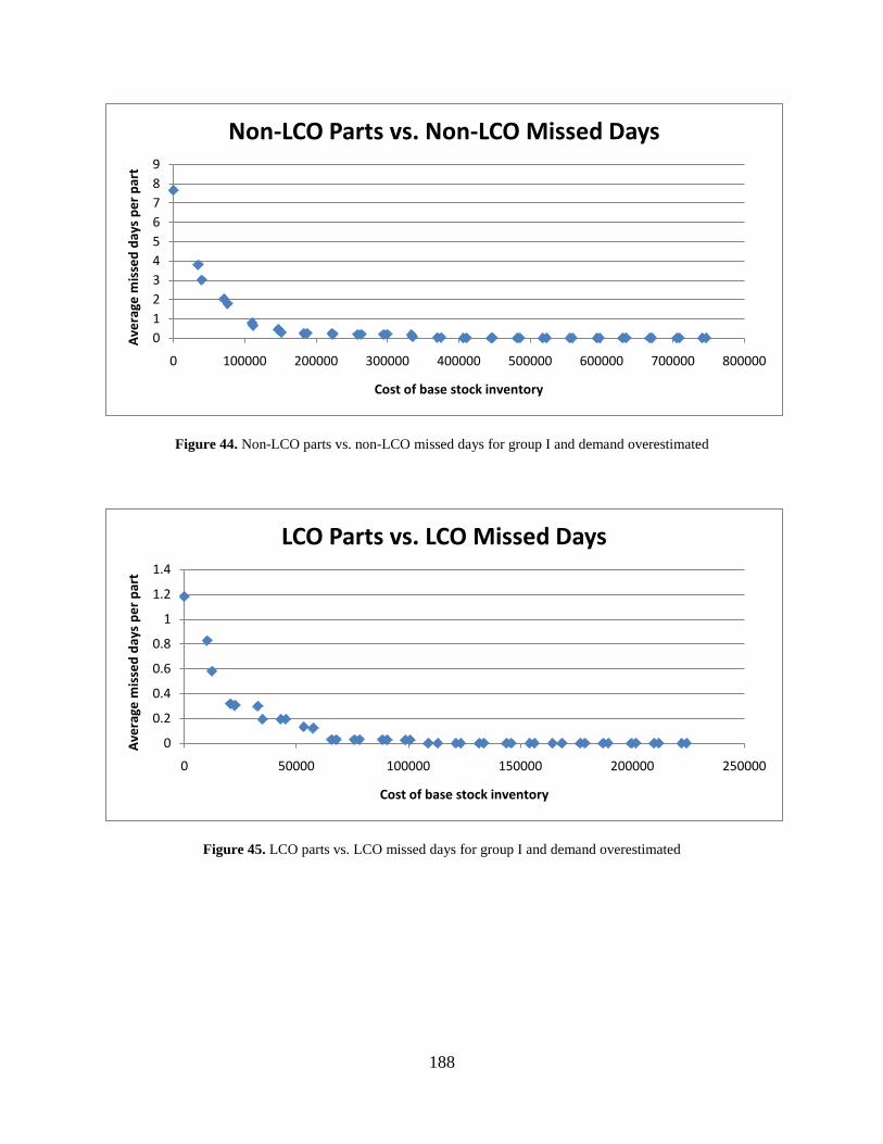
188
Figure 44. Non-LCO parts vs. non-LCO missed days for group I and demand overestimated
Figure 45. LCO parts vs. LCO missed days for group I and demand overestimated
0123456789
0 100000 200000 300000 400000 500000 600000 700000 800000
Ave
rage
mis
sed
days
per
par
t
Cost of base stock inventory
Non-LCO Parts vs. Non-LCO Missed Days
0
0.2
0.4
0.6
0.8
1
1.2
1.4
0 50000 100000 150000 200000 250000
Ave
rage
mis
sed
days
per
par
t
Cost of base stock inventory
LCO Parts vs. LCO Missed Days

189
Table 56. Simulation results for LCO parts in group I and demand overestimated
b Cost Average LCO Missed 0 $ - 1.183
0.5 $ 10,192.13 0.828 1 $ 12,355.96 0.581
1.5 $ 20,459.01 0.320 2 $ 22,622.84 0.305
2.5 $ 32,814.97 0.299 3 $ 34,978.80 0.195
3.5 $ 43,081.85 0.195 4 $ 45,245.68 0.195
4.5 $ 53,348.73 0.134 5 $ 57,601.64 0.122
5.5 $ 65,704.69 0.029 6 $ 67,868.52 0.029
6.5 $ 75,971.57 0.029 7 $ 78,135.40 0.029
7.5 $ 88,327.53 0.029 8 $ 90,491.36 0.026
8.5 $ 98,594.41 0.026 9 $ 100,758.24 0.026
9.5 $ 108,861.29 0.000
C.4.3 Group II, Demand Underestimated
Table 57. Simulation results for all parts in group II and demand underestimated
b Cost Average Non-LCO Missed Average LCO Missed 0 $ - 2.673 0.080
0.5 $ 40,225.61 1.560 0.013 1 $ 42,013.52 1.309 0.013
1.5 $ 67,987.98 1.022 0.013 2 $ 73,660.13 0.930 0.013
2.5 $ 99,439.16 0.863 0.013 3 $ 110,914.38 0.833 0.013
3.5 $ 131,074.96 0.819 0.013 4 $ 133,346.48 0.707 0.013
4.5 $ 168,393.40 0.639 0.013
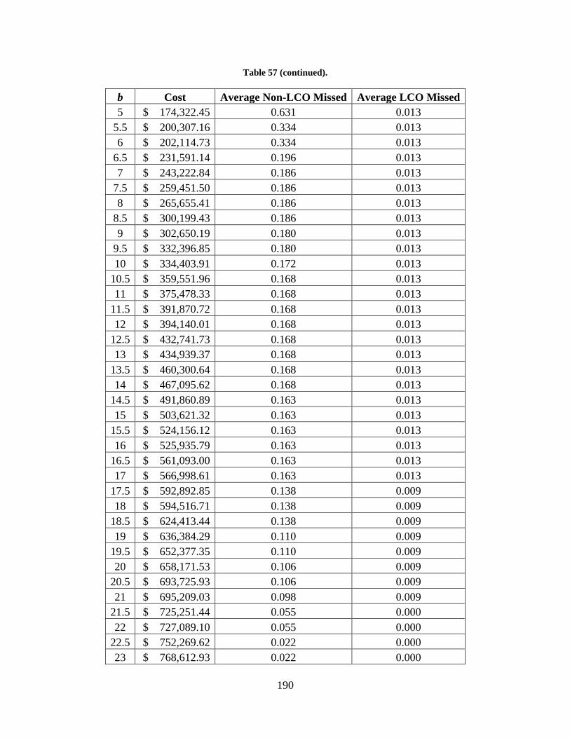
190
Table 57 (continued).
b Cost Average Non-LCO Missed Average LCO Missed 5 $ 174,322.45 0.631 0.013
5.5 $ 200,307.16 0.334 0.013 6 $ 202,114.73 0.334 0.013
6.5 $ 231,591.14 0.196 0.013 7 $ 243,222.84 0.186 0.013
7.5 $ 259,451.50 0.186 0.013 8 $ 265,655.41 0.186 0.013
8.5 $ 300,199.43 0.186 0.013 9 $ 302,650.19 0.180 0.013
9.5 $ 332,396.85 0.180 0.013 10 $ 334,403.91 0.172 0.013
10.5 $ 359,551.96 0.168 0.013 11 $ 375,478.33 0.168 0.013
11.5 $ 391,870.72 0.168 0.013 12 $ 394,140.01 0.168 0.013
12.5 $ 432,741.73 0.168 0.013 13 $ 434,939.37 0.168 0.013
13.5 $ 460,300.64 0.168 0.013 14 $ 467,095.62 0.168 0.013
14.5 $ 491,860.89 0.163 0.013 15 $ 503,621.32 0.163 0.013
15.5 $ 524,156.12 0.163 0.013 16 $ 525,935.79 0.163 0.013
16.5 $ 561,093.00 0.163 0.013 17 $ 566,998.61 0.163 0.013
17.5 $ 592,892.85 0.138 0.009 18 $ 594,516.71 0.138 0.009
18.5 $ 624,413.44 0.138 0.009 19 $ 636,384.29 0.110 0.009
19.5 $ 652,377.35 0.110 0.009 20 $ 658,171.53 0.106 0.009
20.5 $ 693,725.93 0.106 0.009 21 $ 695,209.03 0.098 0.009
21.5 $ 725,251.44 0.055 0.000 22 $ 727,089.10 0.055 0.000
22.5 $ 752,269.62 0.022 0.000 23 $ 768,612.93 0.022 0.000

191
Table 57 (continued).
b Cost Average Non-LCO Missed Average LCO Missed 23.5 $ 784,436.59 0.022 0.000 24 $ 786,552.71 0.022 0.000
24.5 $ 825,143.71 0.022 0.000 25 $ 827,751.42 0.022 0.000
25.5 $ 853,283.52 0.022 0.000 26 $ 859,378.28 0.022 0.000
26.5 $ 884,944.62 0.018 0.000 27 $ 896,871.17 0.018 0.000
27.5 $ 916,745.43 0.018 0.000 28 $ 919,084.38 0.018 0.000
28.5 $ 953,679.87 0.018 0.000 29 $ 959,933.49 0.018 0.000
29.5 $ 985,677.85 0.018 0.000 30 $ 987,815.27 0.018 0.000
30.5 $ 1,017,274.39 0.018 0.000 31 $ 1,028,606.41 0.018 0.000
31.5 $ 1,045,073.33 0.018 0.000 32 $ 1,050,910.16 0.018 0.000
32.5 $ 1,085,928.26 0.018 0.000 33 $ 1,087,855.19 0.018 0.000
33.5 $ 1,117,877.85 0.018 0.000 34 $ 1,120,369.64 0.010 0.000
34.5 $ 1,145,709.33 0.010 0.000 35 $ 1,161,198.62 0.010 0.000
35.5 $ 1,177,351.72 0.010 0.000 36 $ 1,179,058.11 0.010 0.000
36.5 $ 1,218,661.14 0.010 0.000 37 $ 1,220,194.12 0.010 0.000
37.5 $ 1,245,940.64 0.002 0.000 38 $ 1,252,539.73 0.002 0.000
38.5 $ 1,277,670.33 0.002 0.000 39 $ 1,289,499.51 0.002 0.000
39.5 $ 1,309,441.41 0.002 0.000 40 $ 1,311,367.04 0.002 0.000
40.5 $ 1,346,032.03 0.002 0.000 41 $ 1,352,797.05 0.002 0.000
41.5 $ 1,378,673.61 0.002 0.000

192
Table 57 (continued).
b Cost Average Non-LCO Missed Average LCO Missed 42 $ 1,380,719.61 0.002 0.000
42.5 $ 1,409,840.33 0.002 0.000 43 $ 1,422,248.38 0.002 0.000
43.5 $ 1,437,632.10 0.002 0.000 44 $ 1,444,069.47 0.002 0.000
44.5 $ 1,478,634.96 0.002 0.000 45 $ 1,480,581.88 0.000 0.000
Figure 46. All parts vs. all non-LCO missed days for group II and demand underestimated
0
0.5
1
1.5
2
2.5
3
0 200000 400000 600000 800000 1000000 1200000 1400000 1600000
Ave
rage
mis
sed
days
per
par
t
Cost of base stock inventory
All Parts vs. All Non-LCO Missed Days

193
Figure 47. All parts vs. all LCO missed days for group II and demand underestimated
Figure 48. Non-LCO parts vs. non-LCO missed days for group II and demand underestimated
00.010.020.030.040.050.060.070.080.09
0 200000 400000 600000 800000 1000000 1200000 1400000 1600000
Ave
rage
mis
sed
days
per
par
t
Cost of base stock inventory
All Parts vs. All LCO Missed Days
0
0.5
1
1.5
2
2.5
3
0 200000 400000 600000 800000 1000000 1200000 1400000 1600000
Ave
rage
mis
sed
days
per
par
t
Cost of base stock inventory
Non-LCO Parts vs. Non-LCO Missed Days
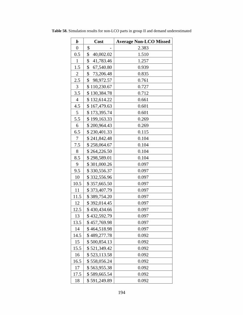
194
Table 58. Simulation results for non-LCO parts in group II and demand underestimated
b Cost Average Non-LCO Missed 0 $ - 2.383
0.5 $ 40,002.02 1.510 1 $ 41,783.46 1.257
1.5 $ 67,540.80 0.939 2 $ 73,206.48 0.835
2.5 $ 98,972.57 0.761 3 $ 110,230.67 0.727
3.5 $ 130,384.78 0.712 4 $ 132,614.22 0.661
4.5 $ 167,479.63 0.601 5 $ 173,395.74 0.601
5.5 $ 199,163.33 0.269 6 $ 200,964.43 0.269
6.5 $ 230,401.33 0.115 7 $ 241,842.48 0.104
7.5 $ 258,064.67 0.104 8 $ 264,226.50 0.104
8.5 $ 298,589.01 0.104 9 $ 301,000.26 0.097
9.5 $ 330,556.37 0.097 10 $ 332,556.96 0.097
10.5 $ 357,665.50 0.097 11 $ 373,407.79 0.097
11.5 $ 389,754.20 0.097 12 $ 392,014.45 0.097
12.5 $ 430,434.66 0.097 13 $ 432,592.79 0.097
13.5 $ 457,769.98 0.097 14 $ 464,518.98 0.097
14.5 $ 489,277.78 0.092 15 $ 500,854.13 0.092
15.5 $ 521,349.42 0.092 16 $ 523,113.58 0.092
16.5 $ 558,056.24 0.092 17 $ 563,955.38 0.092
17.5 $ 589,665.54 0.092 18 $ 591,249.89 0.092

195
Table 58 (continued).
b Cost Average Non-LCO Missed 18.5 $ 621,133.68 0.092 19 $ 632,887.41 0.062
19.5 $ 648,874.00 0.062 20 $ 654,659.14 0.062
20.5 $ 689,992.52 0.062 21 $ 691,469.15 0.062
21.5 $ 721,294.44 0.062 22 $ 723,125.63 0.062
22.5 $ 748,299.68 0.025 23 $ 764,419.40 0.025
23.5 $ 780,236.59 0.025 24 $ 782,310.63 0.025
24.5 $ 820,720.12 0.025 25 $ 823,314.89 0.025
25.5 $ 848,629.87 0.025 26 $ 854,718.16 0.025
26.5 $ 880,242.42 0.020 27 $ 891,987.46 0.020
27.5 $ 911,848.78 0.020 28 $ 914,145.65 0.020
28.5 $ 948,559.63 0.020 29 $ 954,773.74 0.020
29.5 $ 980,327.55 0.020 30 $ 982,458.50 0.020
30.5 $ 1,011,875.54 0.020 31 $ 1,023,026.05 0.020
31.5 $ 1,039,453.46 0.020 32 $ 1,045,274.78 0.020
32.5 $ 1,080,111.37 0.020 33 $ 1,081,998.79 0.020
33.5 $ 1,111,837.37 0.020 34 $ 1,114,283.18 0.012
34.5 $ 1,139,613.83 0.012 35 $ 1,154,921.61 0.012
35.5 $ 1,171,035.20 0.012 36 $ 1,172,732.55 0.012

196
Table 58 (continued).
b Cost Average Non-LCO Missed 36.5 $ 1,212,114.56 0.012 37 $ 1,213,641.07 0.012
37.5 $ 1,239,203.51 0.003 38 $ 1,245,763.09 0.003
38.5 $ 1,270,878.18 0.003 39 $ 1,282,492.81 0.003
39.5 $ 1,302,428.24 0.003 40 $ 1,304,344.83 0.003
40.5 $ 1,338,795.27 0.003 41 $ 1,345,547.35 0.003
41.5 $ 1,371,206.79 0.003 42 $ 1,373,246.32 0.003
42.5 $ 1,402,358.00 0.003 43 $ 1,414,545.03 0.003
43.5 $ 1,429,922.28 0.003 44 $ 1,436,317.57 0.003
44.5 $ 1,470,701.55 0.003 45 $ 1,472,642.00 0.000
Figure 49. LCO parts vs. LCO missed days for group II and demand underestimated
0
0.1
0.2
0.3
0.4
0.5
0.6
0.7
0 1000 2000 3000 4000 5000 6000 7000 8000 9000
Ave
rage
mis
sed
days
per
par
t
Cost of base stock inventory
LCO Parts vs. LCO Missed Days
197
Table 59. Simulation results for LCO parts in group II and demand underestimated
b Cost Average LCO Missed 0 $ - 0.587
0.5 $ 223.59 0.122 1 $ 230.06 0.122
1.5 $ 447.18 0.122 2 $ 453.65 0.122
2.5 $ 466.59 0.122 3 $ 683.71 0.122
3.5 $ 690.18 0.122 4 $ 732.26 0.122
4.5 $ 913.77 0.122 5 $ 926.71 0.122
5.5 $ 1,143.83 0.122 6 $ 1,150.30 0.122
6.5 $ 1,189.81 0.122 7 $ 1,380.36 0.122
7.5 $ 1,386.83 0.122 8 $ 1,428.91 0.122
8.5 $ 1,610.42 0.122 9 $ 1,649.93 0.122
9.5 $ 1,840.48 0.122 10 $ 1,846.95 0.122
10.5 $ 1,886.46 0.122 11 $ 2,070.54 0.122
11.5 $ 2,116.52 0.122 12 $ 2,125.56 0.122
12.5 $ 2,307.07 0.122 13 $ 2,346.58 0.122
13.5 $ 2,530.66 0.122 14 $ 2,576.64 0.122
14.5 $ 2,583.11 0.122 15 $ 2,767.19 0.122
15.5 $ 2,806.70 0.122 16 $ 2,822.21 0.122
16.5 $ 3,036.76 0.122 17 $ 3,043.23 0.122
17.5 $ 3,227.31 0.087 18 $ 3,266.82 0.087
198
Table 59 (continued).
b Cost Average LCO Missed 18.5 $ 3,279.76 0.087 19 $ 3,496.88 0.087
19.5 $ 3,503.35 0.087 20 $ 3,512.39 0.087
20.5 $ 3,733.41 0.087 21 $ 3,739.88 0.087
21.5 $ 3,957.00 0.000
C.4.4 Group II, Demand Overestimated
Table 60. Simulation results for all parts in group II and demand overestimated
b Cost Average Non-LCO Missed Average LCO Missed 0 $ - 2.673 0.080
0.5 $ 40,927.82 1.449 0.013 1 $ 47,600.52 1.161 0.013
1.5 $ 83,573.49 0.785 0.013 2 $ 90,250.09 0.747 0.013
2.5 $ 126,316.13 0.737 0.013 3 $ 132,897.32 0.676 0.013
3.5 $ 168,930.24 0.663 0.013 4 $ 175,504.70 0.645 0.013
4.5 $ 216,008.51 0.466 0.013 5 $ 218,221.12 0.466 0.013
5.5 $ 258,982.55 0.159 0.013 6 $ 261,200.21 0.159 0.013
6.5 $ 301,781.23 0.125 0.013 7 $ 303,792.05 0.125 0.013
7.5 $ 344,289.08 0.121 0.013 8 $ 350,887.54 0.121 0.013
8.5 $ 386,984.97 0.115 0.013 9 $ 393,602.19 0.115 0.013
9.5 $ 429,709.38 0.100 0.013 10 $ 436,213.82 0.065 0.009

199
Table 60 (continued).
b Cost Average Non-LCO Missed Average LCO Missed 10.5 $ 472,585.50 0.058 0.009 11 $ 479,190.43 0.058 0.009
11.5 $ 519,680.95 0.058 0.009 12 $ 521,826.94 0.015 0.000
12.5 $ 562,425.15 0.012 0.000 13 $ 564,642.90 0.012 0.000
13.5 $ 604,948.85 0.012 0.000 14 $ 607,153.31 0.012 0.000
14.5 $ 647,670.09 0.012 0.000 15 $ 654,248.71 0.012 0.000
15.5 $ 690,724.14 0.012 0.000 16 $ 697,300.25 0.012 0.000
16.5 $ 733,218.70 0.012 0.000 17 $ 739,891.40 0.012 0.000
17.5 $ 775,872.52 0.012 0.000 18 $ 782,542.53 0.012 0.000
18.5 $ 823,159.16 0.012 0.000 19 $ 825,269.63 0.009 0.000
19.5 $ 865,808.73 0.009 0.000 20 $ 867,806.30 0.000 0.000
Figure 50. All parts vs. all non-LCO missed days for group II and demand overestimated
0
0.5
1
1.5
2
2.5
3
0 100000 200000 300000 400000 500000 600000 700000 800000 900000
Ave
rage
mis
sed
days
per
par
t
Cost of base stock inventory
All Parts vs. All Non-LCO Missed Days
200
Figure 51. All parts vs. all LCO missed days for group II and demand overestimated
Figure 52. Non-LCO parts vs. non-LCO missed days for group II and demand overestimated
00.010.020.030.040.050.060.070.080.09
0 100000 200000 300000 400000 500000 600000 700000 800000 900000
Ave
rage
mis
sed
days
per
par
t
Cost of base stock inventory
All Parts vs. All LCO Missed Days
0
0.5
1
1.5
2
2.5
3
0 100000 200000 300000 400000 500000 600000 700000 800000 900000
Ave
rage
mis
sed
days
per
par
t
Cost of base stock inventory
Non-LCO Parts vs. Non-LCO Missed Days
201
Table 61. Simulation results for non-LCO parts in group II and demand overestimated
b Cost Average Non-LCO Missed 0 $ - 2.383
0.5 $ 40,671.19 1.385 1 $ 47,268.77 1.167
1.5 $ 83,024.62 0.748 2 $ 89,622.20 0.707
2.5 $ 125,471.12 0.695 3 $ 131,977.19 0.627
3.5 $ 167,762.52 0.613 4 $ 174,288.43 0.608
4.5 $ 214,542.08 0.417 5 $ 216,715.18 0.417
5.5 $ 257,219.98 0.073 6 $ 259,362.52 0.073
6.5 $ 299,728.99 0.036 7 $ 301,664.69 0.036
7.5 $ 341,938.13 0.031 8 $ 348,464.04 0.031
8.5 $ 384,311.31 0.025 9 $ 390,879.98 0.025
9.5 $ 426,739.58 0.016 10 $ 433,201.94 0.012
10.5 $ 469,323.46 0.003 11 $ 475,849.37 0.003
11.5 $ 516,122.77 0.003 12 $ 518,193.64 0.003
12.5 $ 558,570.83 0.000
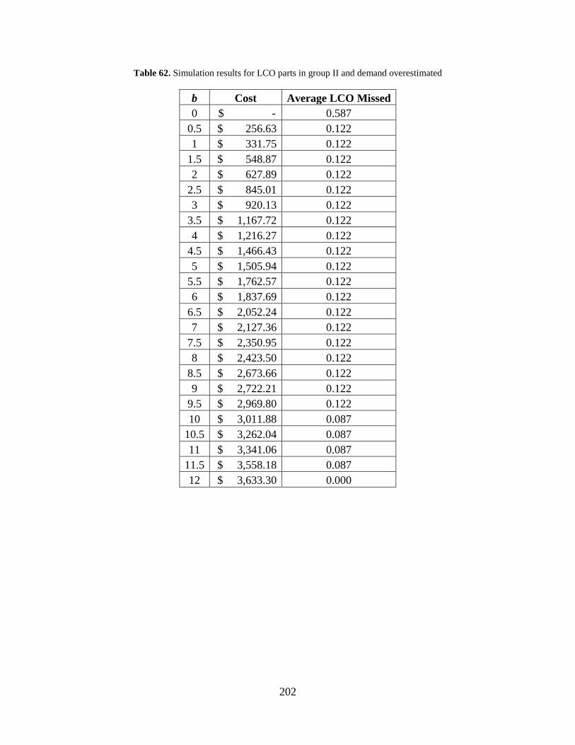
202
Table 62. Simulation results for LCO parts in group II and demand overestimated
b Cost Average LCO Missed 0 $ - 0.587
0.5 $ 256.63 0.122 1 $ 331.75 0.122
1.5 $ 548.87 0.122 2 $ 627.89 0.122
2.5 $ 845.01 0.122 3 $ 920.13 0.122
3.5 $ 1,167.72 0.122 4 $ 1,216.27 0.122
4.5 $ 1,466.43 0.122 5 $ 1,505.94 0.122
5.5 $ 1,762.57 0.122 6 $ 1,837.69 0.122
6.5 $ 2,052.24 0.122 7 $ 2,127.36 0.122
7.5 $ 2,350.95 0.122 8 $ 2,423.50 0.122
8.5 $ 2,673.66 0.122 9 $ 2,722.21 0.122
9.5 $ 2,969.80 0.122 10 $ 3,011.88 0.087
10.5 $ 3,262.04 0.087 11 $ 3,341.06 0.087
11.5 $ 3,558.18 0.087 12 $ 3,633.30 0.000
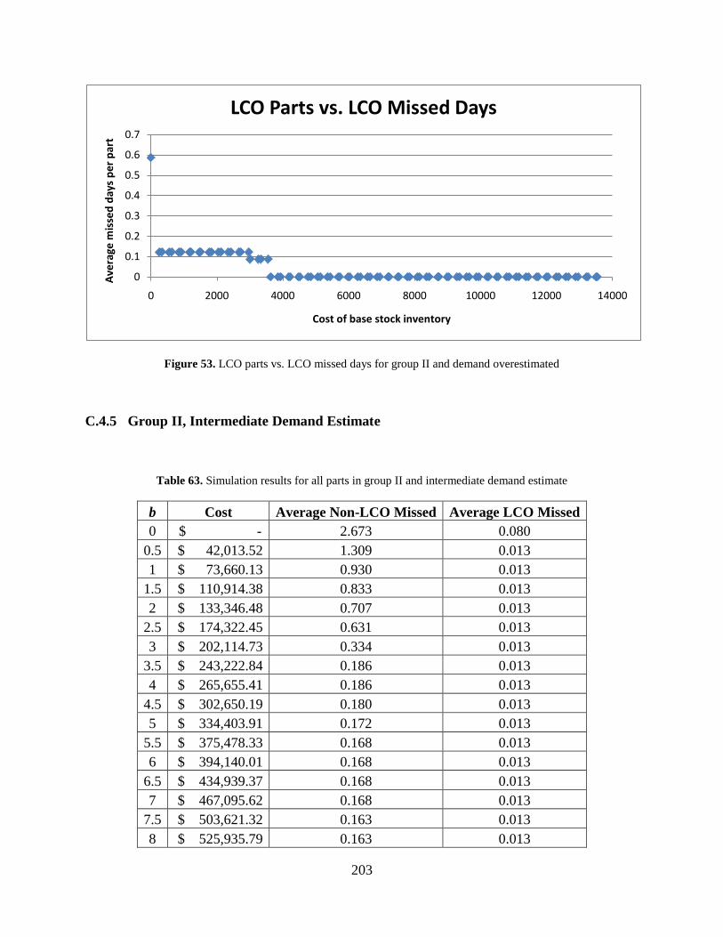
203
Figure 53. LCO parts vs. LCO missed days for group II and demand overestimated
C.4.5 Group II, Intermediate Demand Estimate
Table 63. Simulation results for all parts in group II and intermediate demand estimate
b Cost Average Non-LCO Missed Average LCO Missed 0 $ - 2.673 0.080
0.5 $ 42,013.52 1.309 0.013 1 $ 73,660.13 0.930 0.013
1.5 $ 110,914.38 0.833 0.013 2 $ 133,346.48 0.707 0.013
2.5 $ 174,322.45 0.631 0.013 3 $ 202,114.73 0.334 0.013
3.5 $ 243,222.84 0.186 0.013 4 $ 265,655.41 0.186 0.013
4.5 $ 302,650.19 0.180 0.013 5 $ 334,403.91 0.172 0.013
5.5 $ 375,478.33 0.168 0.013 6 $ 394,140.01 0.168 0.013
6.5 $ 434,939.37 0.168 0.013 7 $ 467,095.62 0.168 0.013
7.5 $ 503,621.32 0.163 0.013 8 $ 525,935.79 0.163 0.013
0
0.1
0.2
0.3
0.4
0.5
0.6
0.7
0 2000 4000 6000 8000 10000 12000 14000
Ave
rage
mis
sed
days
per
par
t
Cost of base stock inventory
LCO Parts vs. LCO Missed Days
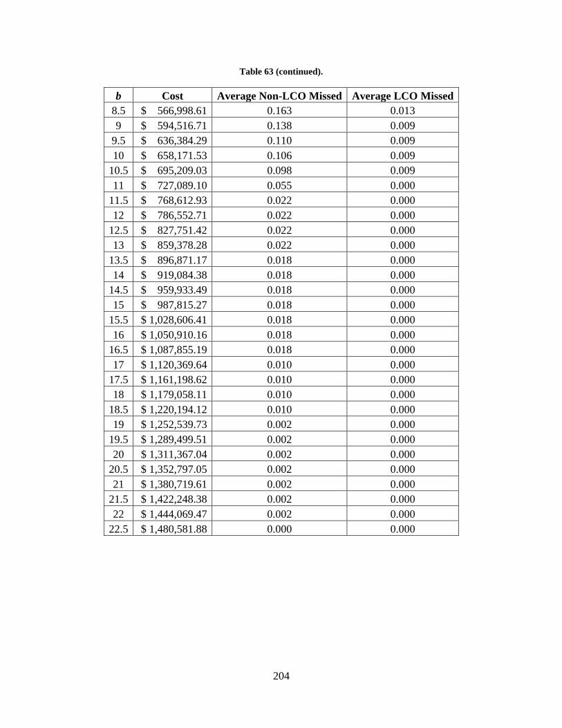
204
Table 63 (continued).
b Cost Average Non-LCO Missed Average LCO Missed 8.5 $ 566,998.61 0.163 0.013 9 $ 594,516.71 0.138 0.009
9.5 $ 636,384.29 0.110 0.009 10 $ 658,171.53 0.106 0.009
10.5 $ 695,209.03 0.098 0.009 11 $ 727,089.10 0.055 0.000
11.5 $ 768,612.93 0.022 0.000 12 $ 786,552.71 0.022 0.000
12.5 $ 827,751.42 0.022 0.000 13 $ 859,378.28 0.022 0.000
13.5 $ 896,871.17 0.018 0.000 14 $ 919,084.38 0.018 0.000
14.5 $ 959,933.49 0.018 0.000 15 $ 987,815.27 0.018 0.000
15.5 $ 1,028,606.41 0.018 0.000 16 $ 1,050,910.16 0.018 0.000
16.5 $ 1,087,855.19 0.018 0.000 17 $ 1,120,369.64 0.010 0.000
17.5 $ 1,161,198.62 0.010 0.000 18 $ 1,179,058.11 0.010 0.000
18.5 $ 1,220,194.12 0.010 0.000 19 $ 1,252,539.73 0.002 0.000
19.5 $ 1,289,499.51 0.002 0.000 20 $ 1,311,367.04 0.002 0.000
20.5 $ 1,352,797.05 0.002 0.000 21 $ 1,380,719.61 0.002 0.000
21.5 $ 1,422,248.38 0.002 0.000 22 $ 1,444,069.47 0.002 0.000
22.5 $ 1,480,581.88 0.000 0.000

205
Figure 54. All parts vs. all non-LCO missed days for group II and intermediate demand estimate
Figure 55. All parts vs. all LCO missed days for group II and intermediate demand estimate
0
0.5
1
1.5
2
2.5
3
0 200000 400000 600000 800000 1000000 1200000 1400000 1600000 1800000
Ave
rage
mis
sed
days
per
par
t
Cost of base stock inventory
All Parts vs. All Non-LCO Missed Days
00.010.020.030.040.050.060.070.080.09
0 200000 400000 600000 800000 1000000 1200000 1400000 1600000 1800000
Ave
rage
mis
sed
days
per
par
t
Cost of base stock inventory
All Parts vs. All LCO Missed Days

206
Table 64. Simulation results for non-LCO parts in group II and intermediate demand estimate
b Cost Average Non-LCO Missed 0 $ - 2.383
0.5 $ 41,783.46 1.257 1 $ 73,206.48 0.835
1.5 $ 110,230.67 0.727 2 $ 132,614.22 0.661
2.5 $ 173,395.74 0.601 3 $ 200,964.43 0.269
3.5 $ 241,842.48 0.104 4 $ 264,226.50 0.104
4.5 $ 301,000.26 0.097 5 $ 332,556.96 0.097
5.5 $ 373,407.79 0.097 6 $ 392,014.45 0.097
6.5 $ 432,592.79 0.097 7 $ 464,518.98 0.097
7.5 $ 500,854.13 0.092 8 $ 523,113.58 0.092
8.5 $ 563,955.38 0.092 9 $ 591,249.89 0.092
9.5 $ 632,887.41 0.062 10 $ 654,659.14 0.062
10.5 $ 691,469.15 0.062 11 $ 723,125.63 0.062
11.5 $ 764,419.40 0.025 12 $ 782,310.63 0.025
12.5 $ 823,314.89 0.025 13 $ 854,718.16 0.025
13.5 $ 891,987.46 0.020 14 $ 914,145.65 0.020
14.5 $ 954,773.74 0.020 15 $ 982,458.50 0.020
15.5 $ 1,023,026.05 0.020 16 $ 1,045,274.78 0.020
16.5 $ 1,081,998.79 0.020 17 $ 1,114,283.18 0.012
17.5 $ 1,154,921.61 0.012 18 $ 1,172,732.55 0.012

207
Table 64 (continued).
b Cost Average Non-LCO Missed 18.5 $ 1,213,641.07 0.012 19 $ 1,245,763.09 0.003
19.5 $ 1,282,492.81 0.003 20 $ 1,304,344.83 0.003
20.5 $ 1,345,547.35 0.003 21 $ 1,373,246.32 0.003
21.5 $ 1,414,545.03 0.003 22 $ 1,436,317.57 0.003
22.5 $ 1,472,642.00 0.000
Figure 56. Non-LCO parts vs. non-LCO missed days for group II and intermediate demand estimate
0
0.5
1
1.5
2
2.5
3
0 200000 400000 600000 800000 1000000 1200000 1400000 1600000 1800000
Ave
rage
mis
sed
days
per
par
t
Cost of base stock inventory
Non-LCO Parts vs. Non-LCO Missed Days
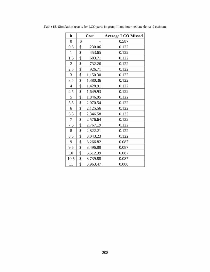
208
Table 65. Simulation results for LCO parts in group II and intermediate demand estimate
b Cost Average LCO Missed 0 $ - 0.587
0.5 $ 230.06 0.122 1 $ 453.65 0.122
1.5 $ 683.71 0.122 2 $ 732.26 0.122
2.5 $ 926.71 0.122 3 $ 1,150.30 0.122
3.5 $ 1,380.36 0.122 4 $ 1,428.91 0.122
4.5 $ 1,649.93 0.122 5 $ 1,846.95 0.122
5.5 $ 2,070.54 0.122 6 $ 2,125.56 0.122
6.5 $ 2,346.58 0.122 7 $ 2,576.64 0.122
7.5 $ 2,767.19 0.122 8 $ 2,822.21 0.122
8.5 $ 3,043.23 0.122 9 $ 3,266.82 0.087
9.5 $ 3,496.88 0.087 10 $ 3,512.39 0.087
10.5 $ 3,739.88 0.087 11 $ 3,963.47 0.000
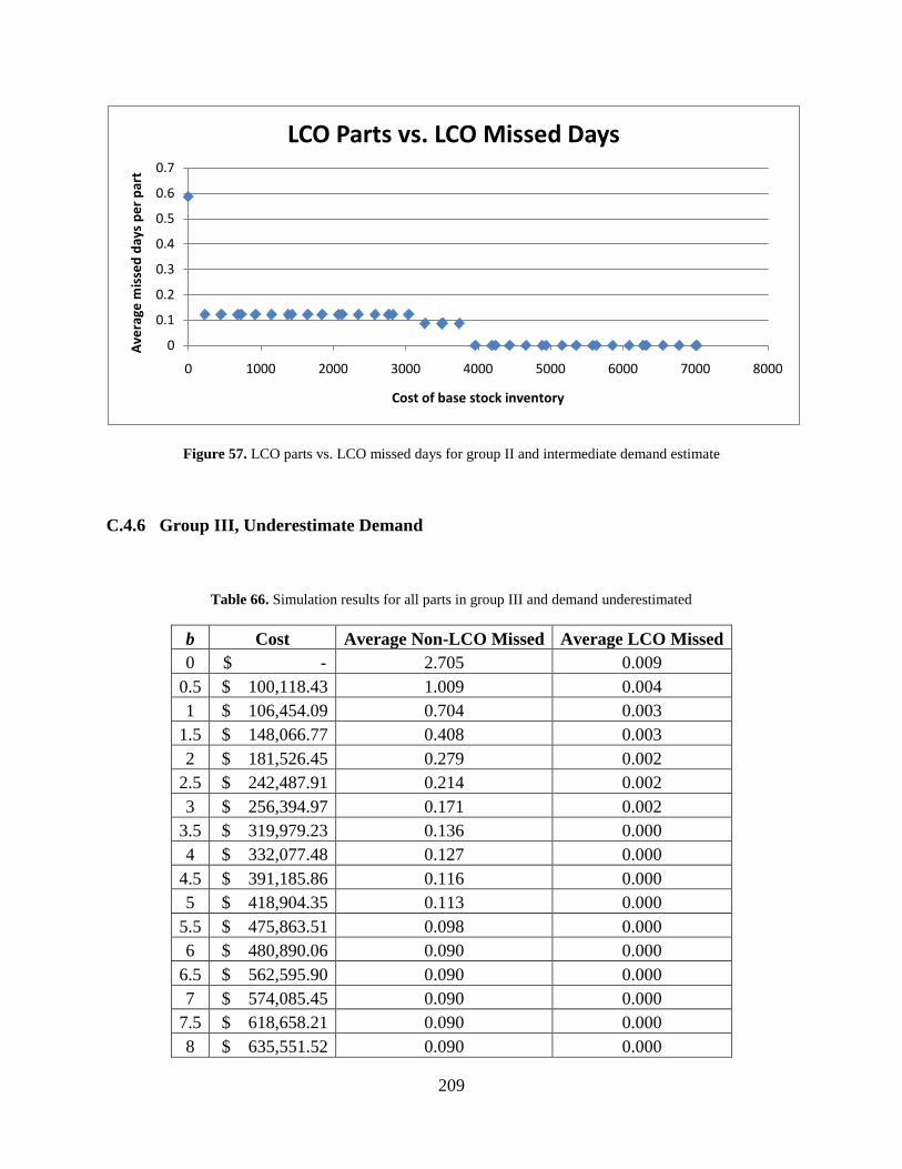
209
Figure 57. LCO parts vs. LCO missed days for group II and intermediate demand estimate
C.4.6 Group III, Underestimate Demand
Table 66. Simulation results for all parts in group III and demand underestimated
b Cost Average Non-LCO Missed Average LCO Missed 0 $ - 2.705 0.009
0.5 $ 100,118.43 1.009 0.004 1 $ 106,454.09 0.704 0.003
1.5 $ 148,066.77 0.408 0.003 2 $ 181,526.45 0.279 0.002
2.5 $ 242,487.91 0.214 0.002 3 $ 256,394.97 0.171 0.002
3.5 $ 319,979.23 0.136 0.000 4 $ 332,077.48 0.127 0.000
4.5 $ 391,185.86 0.116 0.000 5 $ 418,904.35 0.113 0.000
5.5 $ 475,863.51 0.098 0.000 6 $ 480,890.06 0.090 0.000
6.5 $ 562,595.90 0.090 0.000 7 $ 574,085.45 0.090 0.000
7.5 $ 618,658.21 0.090 0.000 8 $ 635,551.52 0.090 0.000
0
0.1
0.2
0.3
0.4
0.5
0.6
0.7
0 1000 2000 3000 4000 5000 6000 7000 8000
Ave
rage
mis
sed
days
per
par
t
Cost of base stock inventory
LCO Parts vs. LCO Missed Days
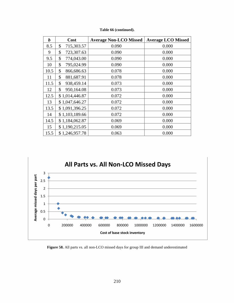
210
Table 66 (continued).
b Cost Average Non-LCO Missed Average LCO Missed 8.5 $ 715,303.57 0.090 0.000 9 $ 723,307.63 0.090 0.000
9.5 $ 774,043.00 0.090 0.000 10 $ 795,024.99 0.090 0.000
10.5 $ 866,686.63 0.078 0.000 11 $ 881,687.91 0.078 0.000
11.5 $ 938,459.14 0.073 0.000 12 $ 950,164.08 0.073 0.000
12.5 $ 1,014,446.87 0.072 0.000 13 $ 1,047,646.27 0.072 0.000
13.5 $ 1,091,396.25 0.072 0.000 14 $ 1,103,189.66 0.072 0.000
14.5 $ 1,184,062.87 0.069 0.000 15 $ 1,190,215.05 0.069 0.000
15.5 $ 1,246,957.78 0.063 0.000
Figure 58. All parts vs. all non-LCO missed days for group III and demand underestimated
0
0.5
1
1.5
2
2.5
3
0 200000 400000 600000 800000 1000000 1200000 1400000 1600000
Ave
rage
mis
sed
days
per
par
t
Cost of base stock inventory
All Parts vs. All Non-LCO Missed Days
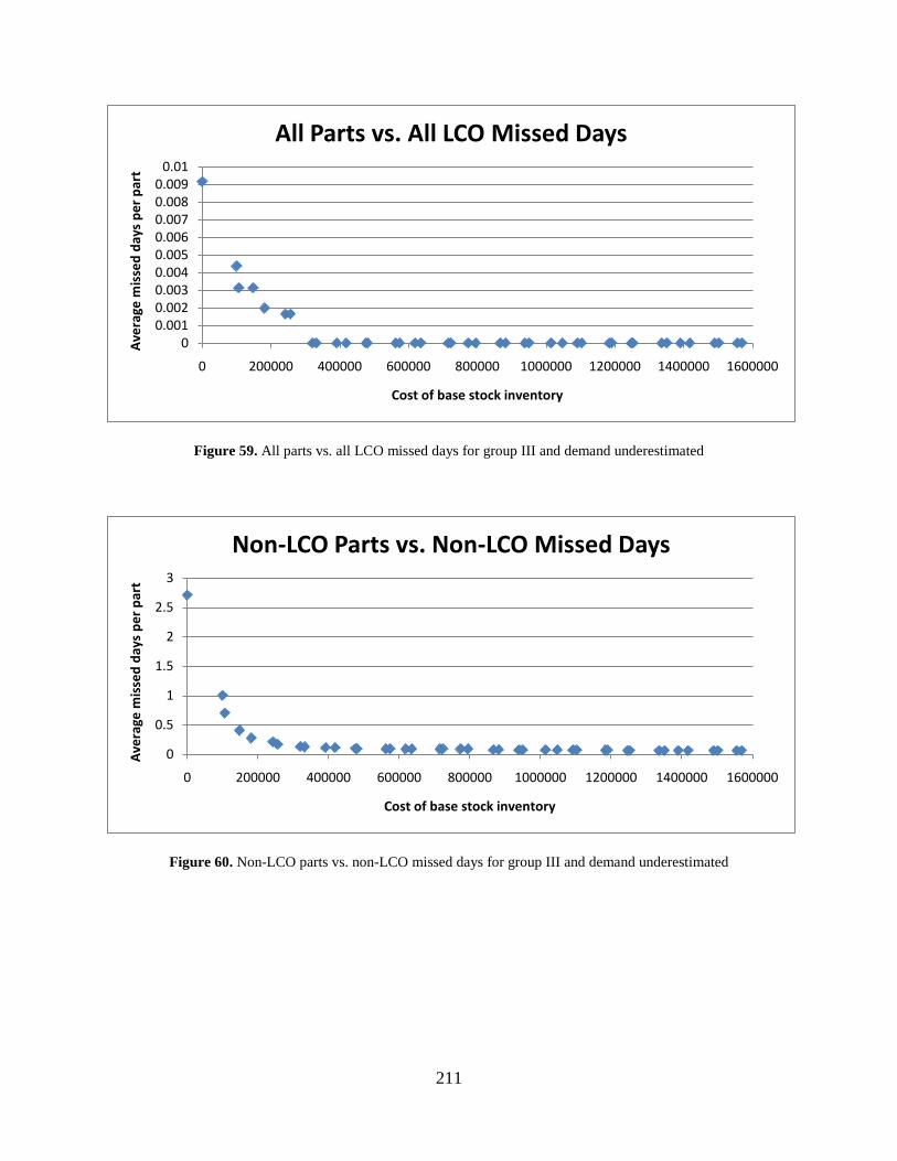
211
Figure 59. All parts vs. all LCO missed days for group III and demand underestimated
Figure 60. Non-LCO parts vs. non-LCO missed days for group III and demand underestimated
00.0010.0020.0030.0040.0050.0060.0070.0080.009
0.01
0 200000 400000 600000 800000 1000000 1200000 1400000 1600000
Ave
rage
mis
sed
days
per
par
t
Cost of base stock inventory
All Parts vs. All LCO Missed Days
0
0.5
1
1.5
2
2.5
3
0 200000 400000 600000 800000 1000000 1200000 1400000 1600000
Ave
rage
mis
sed
days
per
par
t
Cost of base stock inventory
Non-LCO Parts vs. Non-LCO Missed Days

212
Table 67. Simulation results for non-LCO parts in group III and demand underestimated
b Cost Average Non-LCO Missed 0 $ - 2.710
0.5 $ 100,114.69 1.003 1 $ 106,446.61 0.703
1.5 $ 148,055.55 0.406 2 $ 181,511.49 0.277
2.5 $ 242,469.21 0.212 3 $ 256,372.53 0.168
3.5 $ 319,953.05 0.133 4 $ 332,047.56 0.123
4.5 $ 391,152.20 0.114 5 $ 418,866.95 0.114
5.5 $ 475,822.37 0.098 6 $ 480,845.18 0.091
6.5 $ 562,547.28 0.091 7 $ 574,033.09 0.091
7.5 $ 618,602.11 0.090 8 $ 635,491.68 0.090
8.5 $ 715,239.99 0.090 9 $ 723,240.31 0.090
9.5 $ 773,971.94 0.090 10 $ 794,950.19 0.090
10.5 $ 866,608.09 0.078 11 $ 881,605.63 0.078
11.5 $ 938,373.12 0.073 12 $ 950,074.32 0.073
12.5 $ 1,014,353.37 0.073 13 $ 1,047,549.03 0.073
13.5 $ 1,091,295.27 0.073 14 $ 1,103,084.94 0.073
14.5 $ 1,183,954.41 0.070 15 $ 1,190,102.85 0.070
15.5 $ 1,246,841.84 0.064

213
Figure 61. LCO parts vs. LCO missed days for group III and demand underestimated
Table 68. Simulation results for LCO parts in group III and demand underestimated
b Cost Average LCO Missed 0 $ - 0.407
0.5 $ 3.74 0.407 1 $ 7.48 0.233
1.5 $ 11.22 0.233 2 $ 14.96 0.233
2.5 $ 18.70 0.233 3 $ 22.44 0.233
3.5 $ 26.18 0.000
00.05
0.10.15
0.20.25
0.30.35
0.40.45
0 20 40 60 80 100 120 140 160
Ave
rage
mis
sed
days
per
par
t
Cost of base stock inventory
LCO Parts vs. LCO Missed Days
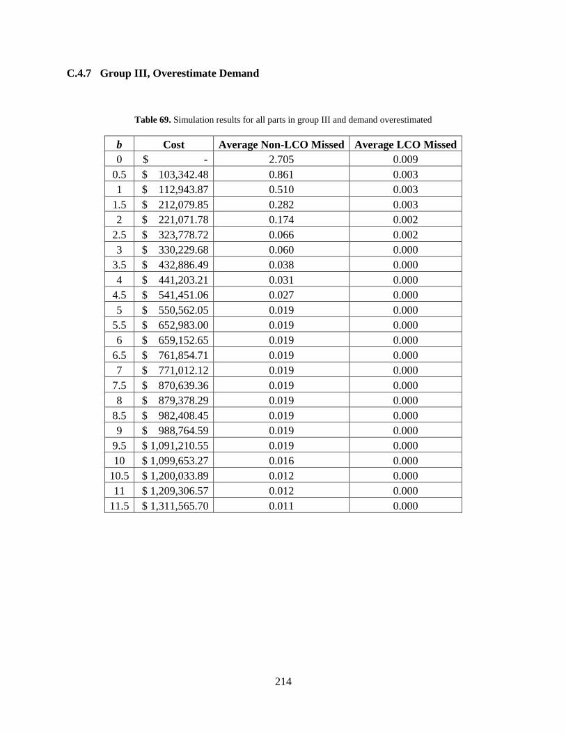
214
C.4.7 Group III, Overestimate Demand
Table 69. Simulation results for all parts in group III and demand overestimated
b Cost Average Non-LCO Missed Average LCO Missed 0 $ - 2.705 0.009
0.5 $ 103,342.48 0.861 0.003 1 $ 112,943.87 0.510 0.003
1.5 $ 212,079.85 0.282 0.003 2 $ 221,071.78 0.174 0.002
2.5 $ 323,778.72 0.066 0.002 3 $ 330,229.68 0.060 0.000
3.5 $ 432,886.49 0.038 0.000 4 $ 441,203.21 0.031 0.000
4.5 $ 541,451.06 0.027 0.000 5 $ 550,562.05 0.019 0.000
5.5 $ 652,983.00 0.019 0.000 6 $ 659,152.65 0.019 0.000
6.5 $ 761,854.71 0.019 0.000 7 $ 771,012.12 0.019 0.000
7.5 $ 870,639.36 0.019 0.000 8 $ 879,378.29 0.019 0.000
8.5 $ 982,408.45 0.019 0.000 9 $ 988,764.59 0.019 0.000
9.5 $ 1,091,210.55 0.019 0.000 10 $ 1,099,653.27 0.016 0.000
10.5 $ 1,200,033.89 0.012 0.000 11 $ 1,209,306.57 0.012 0.000
11.5 $ 1,311,565.70 0.011 0.000

215
Figure 62. All parts vs. all non-LCO missed days for group III and demand overestimated
Figure 63. All parts vs. all LCO missed days for group III and demand overestimated
0
0.5
1
1.5
2
2.5
3
0 500000 1000000 1500000 2000000 2500000
Ave
rage
mis
sed
days
per
par
t
Cost of base stock inventory
All Parts vs. All Non-LCO Missed Days
00.0010.0020.0030.0040.0050.0060.0070.0080.009
0.01
0 500000 1000000 1500000 2000000 2500000
Ave
rage
mis
sed
days
per
par
t
Cost of base stock inventory
All Parts vs. All LCO Missed Days
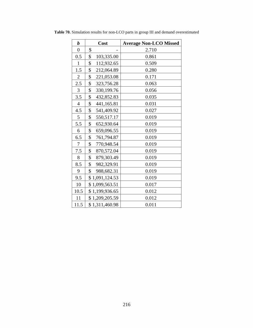
216
Table 70. Simulation results for non-LCO parts in group III and demand overestimated
b Cost Average Non-LCO Missed 0 $ - 2.710
0.5 $ 103,335.00 0.861 1 $ 112,932.65 0.509
1.5 $ 212,064.89 0.280 2 $ 221,053.08 0.171
2.5 $ 323,756.28 0.063 3 $ 330,199.76 0.056
3.5 $ 432,852.83 0.035 4 $ 441,165.81 0.031
4.5 $ 541,409.92 0.027 5 $ 550,517.17 0.019
5.5 $ 652,930.64 0.019 6 $ 659,096.55 0.019
6.5 $ 761,794.87 0.019 7 $ 770,948.54 0.019
7.5 $ 870,572.04 0.019 8 $ 879,303.49 0.019
8.5 $ 982,329.91 0.019 9 $ 988,682.31 0.019
9.5 $ 1,091,124.53 0.019 10 $ 1,099,563.51 0.017
10.5 $ 1,199,936.65 0.012 11 $ 1,209,205.59 0.012
11.5 $ 1,311,460.98 0.011

217
Figure 64. Non-LCO parts vs. non-LCO missed days for group III and demand overestimated
Figure 65. LCO parts vs. LCO missed days for group III and demand overestimated
0
0.5
1
1.5
2
2.5
3
0 500000 1000000 1500000 2000000 2500000
Ave
rage
mis
sed
days
per
par
t
Cost of base stock inventory
Non-LCO Parts vs. Non-LCO Missed Days
00.05
0.10.15
0.20.25
0.30.35
0.40.45
0 20 40 60 80 100 120 140 160 180 200
Ave
rage
mis
sed
days
per
par
t
Cost of base stock inventory
LCO Parts vs. LCO Missed Days

218
Table 71. Simulation results for LCO parts in group III and demand overestimated
b Cost Average LCO Missed 0 $ - 0.407
0.5 $ 7.48 0.233 1 $ 11.22 0.233
1.5 $ 14.96 0.233 2 $ 18.70 0.233
2.5 $ 22.44 0.233 3 $ 29.92 0.000
C.4.8 Group III, Intermediate Demand Estimate
Table 72. Simulation results for all parts in group III and intermediate demand estimate
b Cost Average Non-LCO Missed Average LCO Missed 0 $ - 2.705 0.009
0.5 $ 106,454.09 0.704 0.003 1 $ 181,526.45 0.279 0.002
1.5 $ 256,394.97 0.171 0.002 2 $ 332,077.48 0.127 0.000
2.5 $ 418,904.35 0.113 0.000 3 $ 480,890.06 0.090 0.000
3.5 $ 574,085.45 0.090 0.000 4 $ 635,551.52 0.090 0.000
4.5 $ 723,307.63 0.090 0.000 5 $ 795,024.99 0.090 0.000
5.5 $ 881,687.91 0.078 0.000 6 $ 950,164.08 0.073 0.000
6.5 $ 1,047,646.27 0.072 0.000 7 $ 1,103,189.66 0.072 0.000
7.5 $ 1,190,215.05 0.069 0.000 8 $ 1,253,127.93 0.063 0.000
8.5 $ 1,351,059.56 0.063 0.000 9 $ 1,417,970.07 0.063 0.000
9.5 $ 1,502,234.95 0.063 0.000 10 $ 1,569,390.35 0.063 0.000
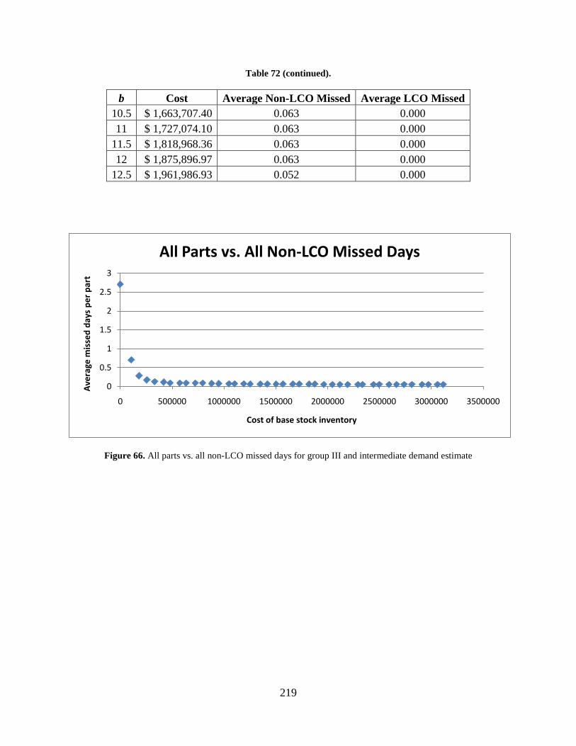
219
Table 72 (continued).
b Cost Average Non-LCO Missed Average LCO Missed 10.5 $ 1,663,707.40 0.063 0.000 11 $ 1,727,074.10 0.063 0.000
11.5 $ 1,818,968.36 0.063 0.000 12 $ 1,875,896.97 0.063 0.000
12.5 $ 1,961,986.93 0.052 0.000
Figure 66. All parts vs. all non-LCO missed days for group III and intermediate demand estimate
0
0.5
1
1.5
2
2.5
3
0 500000 1000000 1500000 2000000 2500000 3000000 3500000
Ave
rage
mis
sed
days
per
par
t
Cost of base stock inventory
All Parts vs. All Non-LCO Missed Days

220
Figure 67. All parts vs. all LCO missed days for group III and intermediate demand estimate
Figure 68. Non-LCO parts vs. non-LCO missed days for group III and intermediate demand estimate
00.0010.0020.0030.0040.0050.0060.0070.0080.009
0.01
0 500000 1000000 1500000 2000000 2500000 3000000 3500000
Ave
rage
mis
sed
days
per
par
t
Cost of base stock inventory
All Parts vs. All LCO Missed Days
0
0.5
1
1.5
2
2.5
3
0 500000 1000000 1500000 2000000 2500000 3000000 3500000
Ave
rage
mis
sed
days
per
par
t
Cost of base stock inventory
Non-LCO Parts vs. Non-LCO Missed Days
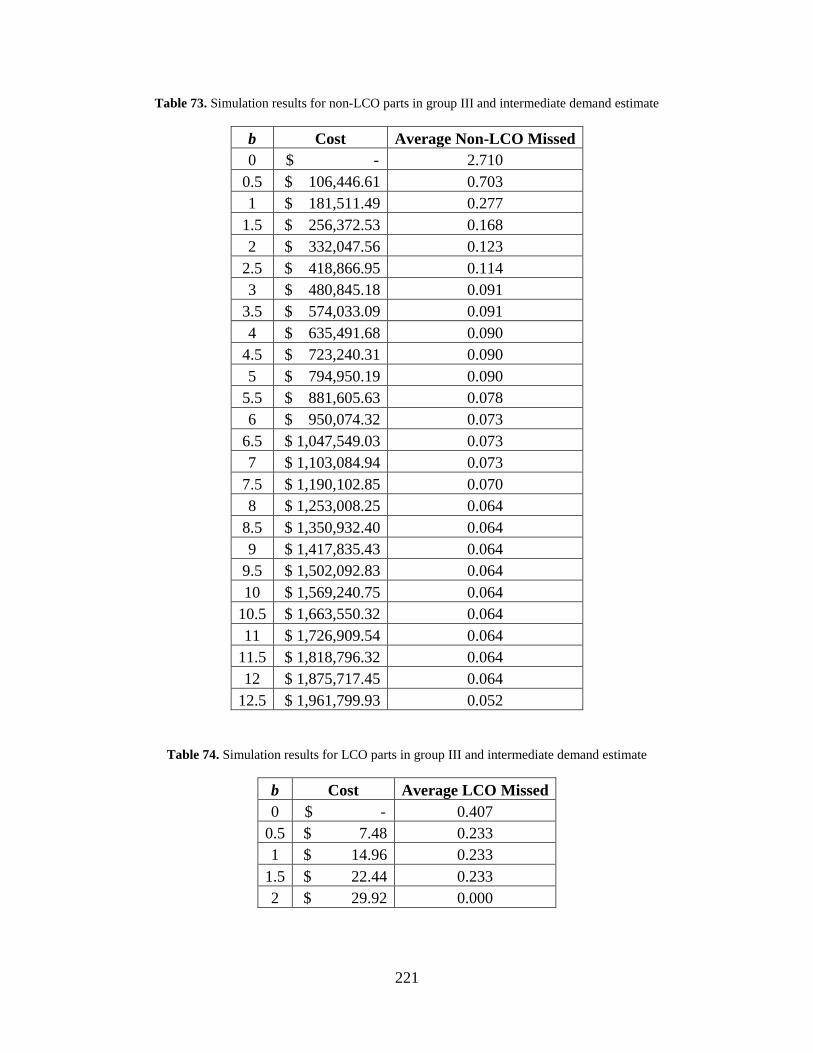
221
Table 73. Simulation results for non-LCO parts in group III and intermediate demand estimate
b Cost Average Non-LCO Missed 0 $ - 2.710
0.5 $ 106,446.61 0.703 1 $ 181,511.49 0.277
1.5 $ 256,372.53 0.168 2 $ 332,047.56 0.123
2.5 $ 418,866.95 0.114 3 $ 480,845.18 0.091
3.5 $ 574,033.09 0.091 4 $ 635,491.68 0.090
4.5 $ 723,240.31 0.090 5 $ 794,950.19 0.090
5.5 $ 881,605.63 0.078 6 $ 950,074.32 0.073
6.5 $ 1,047,549.03 0.073 7 $ 1,103,084.94 0.073
7.5 $ 1,190,102.85 0.070 8 $ 1,253,008.25 0.064
8.5 $ 1,350,932.40 0.064 9 $ 1,417,835.43 0.064
9.5 $ 1,502,092.83 0.064 10 $ 1,569,240.75 0.064
10.5 $ 1,663,550.32 0.064 11 $ 1,726,909.54 0.064
11.5 $ 1,818,796.32 0.064 12 $ 1,875,717.45 0.064
12.5 $ 1,961,799.93 0.052
Table 74. Simulation results for LCO parts in group III and intermediate demand estimate
b Cost Average LCO Missed 0 $ - 0.407
0.5 $ 7.48 0.233 1 $ 14.96 0.233
1.5 $ 22.44 0.233 2 $ 29.92 0.000
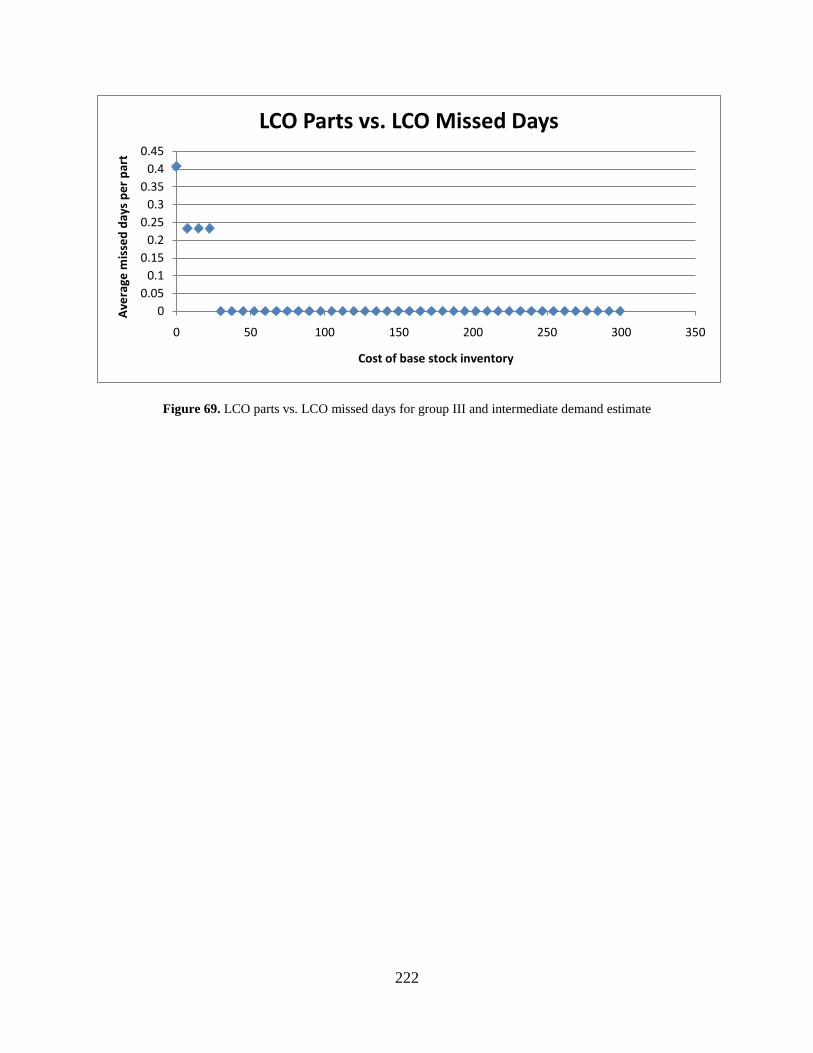
222
Figure 69. LCO parts vs. LCO missed days for group III and intermediate demand estimate
00.05
0.10.15
0.20.25
0.30.35
0.40.45
0 50 100 150 200 250 300 350
Ave
rage
mis
sed
days
per
par
t
Cost of base stock inventory
LCO Parts vs. LCO Missed Days

223
BIBLIOGRAPHY
[1] Aczél, J., & Alsina, C. (1987). Synthesizing judgements: A functional equations approach. Mathematical Modelling, 9(3-5), 311-320.
[2] Aczél, J., & Saaty, T. L. (1983). Procedures for synthesizing ratio judgements. Journal of Mathematical Psychology, 27, 93-102.
[3] Agogino, A. M., Nour-Omid, O., Imaino, W., & Wang, S. S. (1992). Decision-analytic methodology for cost-benefit evaluation of diagnostic testers. IIE Transactions, 24(1), 39-54.
[4] Anderson, T. W. (2003). An introduction to multivariate statistical analysis (3rd ed.). Hoboken, New Jersey: Wiley-Interscience.
[5] Armacost, R. L., Hosseini, J. C., & Pet-Edwards, J. (1999). Using the Analytic Hierarchy
Process as a two-phase integrated decision approach for large nominal groups. Group Decision and Negotiation, 8, 535-555.
[6] Asaro, C. A., & Tierney, T. (2005). Who’s buying who: Mergers and acquisitions of utilities are on the rise. Retrieved January 7, 2011, from http://www.beechercarlson.com/files/pdf/energyarticle.pdf
[7] Basak, I. (1988). When to combine group judgments and when not to in the Analytic Hierarchy Process: A new method. Mathematical and Computer Modelling, 10(6), 395-404.
[8] Basak, I. & Saaty, T. (1993). Group decision making using the Analytic Hierarchy Process. Mathematical and Computer Modelling, 17(4-5), 101-109.
[9] Bond, L. J., Doctor, S. R., Jarrell, D. B., & Bond, J. W. D. (2007). Improved economics of nuclear plant life management. Retrieved April 14, 2011, from http://pmmd.pnnl.gov/program/reports/IAEA-Improved-Economics-100307.pdf
[10] Borenstein, S. (2009). Electricity pricing that reflects its real time cost. Retrieved July 23, 2009, from http://www.nber.org/reporter/2009number1/borenstein.html

224
[11] Braglia, M., Grassi, A., & Montanari, R. (2004). Multi-attribute classification method for spare parts inventory management. Journal of Quality in Maintenance Engineering, 10(1), 55-65.
[12] Casman, E. A., & Fischhoff, B. (2008). Risk communication planning for the aftermath of a plague bioattack. Risk Analysis, 28(5), 1327-1342.
[13] Cohen, M. A., & Ernst, R. (1988). Multi-item classification and generic inventory stock control policies. Production and Inventory Management Journal, 29(3), 6-8.
[14] Creative Decisions Foundation. (n.d.). SuperDecisions software for decision making. Retrieved April 26, 2010, from http://www.superdecisions.com/
[15] Croston, J. D. (1972, September). Forecasting and stock control for intermittent demands. Operational Research Quarterly, 23(3), 289-303.
[16] Duintjer-Tebbens, R. J., Pallansch, M. A., Kew, O. M., Sutter, R. W., Aylward, R. B., Watkins, M., et al. (2008). Uncertainty and sensitivity analyses of a decision analytic model for posteradication polio risk management. Risk Analysis, 28(4), 855-876.
[17] Dunteman, G. H. (1989). Principal components analysis. Newbury Park, California: Sage Publications.
[18] Eleye-Datubo, A. G., Wall, A., Saajedi, A., & Wang, J. (2006). Enabling a powerful
marine and offshore decision-support solution through Bayesian Network Technique. Risk Analysis, 26(3), 695-721.
[19] Energy Policy Act of 1992, 7 U.S.C. § 711 (1992).
[20] Ernst, R., & Cohen, M. A. (1990). Operations related groups (ORGs): A clustering procedure for production / inventory systems. Journal of Operations Management, 9(4), 574-598.
[21] Federal Energy Regulatory Commission. (2010, June 28). Order No. 888. Retrieved March 6, 2011, from http://www.ferc.gov/legal/maj-ord-reg/land-docs/order888.asp
[22] Flores, B. E., Olson, D. L., & Dorai, V. K. (1992). Management of multicriteria inventory classification. Mathematical and Computer Modelling, 16(12), 71-82.
[23] Flores, B. E., & Whybark, D. C. (1987). Implementing multiple criteria ABC analysis. Journal of Operations Management, 7(1-2), 79-85.
[24] Gajpal, P. P., Ganesh, L. S., & Rajendran, C. (1994). Criticality analysis of spare parts using the Analytic Hierarchy Process. International Journal of Production Economics, 35, 293-297.
[25] Hadi-Vencheh, A. (2010). An improvement to multiple criteria ABC inventory classification. European Journal of Operational Research, 201, 962-965.

225
[26] Harvey, J., Bolam, H., Gregory, D., & Erdos, G. (2001). The effectiveness of training to change safety culture and attitudes within a highly regulated environment. Personnel Review, 30(6), 615-636.
[27] Heizer, J., & Render, B. (2011). Operations management (10th ed.). Boston: Prentice Hall.
[28] Hopp, W. J., & Spearman, M. L. (2001). Factory physics: Foundations of manufacturing management (2nd ed.). Boston: Irwin McGraw-Hill.
[29] Howard, R. A., & Matheson, J. E. (2005). Influence diagrams. Decision Analysis, 2(3), 127-143.
[30] Huiskonen, J. (2001). Maintenance spare parts logistics: Special characteristics and
strategic choices. International Journal of Production Economics, 71, 125-133. [31] Johnson, R. A., & Wichern, D. W. (2007). Applied multivariate statistical analysis (6th
ed.). Upper Saddle River, New Jersey: Pearson Prentice Hall. [32] Jolliffe, I. T. (2002). Principal component analysis (2nd ed.). New York: Springer-
Verlag. [33] Keefer, D. L. (2004). Practice abstracts. Interfaces, 34(3), 206-207. [34] Kivimäki, M., & Kalimo, R. (1993). Risk perception among nuclear power plant
personnel: A survey. Risk Analysis, 13(4), 421-424.
[35] Kivimäki, M., Kalimo, R., & Salminen, S. (1995). Perceived nuclear risk, organizational commitment, and appraisals of management: A study of nuclear power plant personnel. Risk Analysis, 15(3), 391-396.
[36] Korpela, J., & Tuominen, M. (1996). Inventory forecasting with a multiple criteria decision tool. International Journal of Production Economics, 45(1-3), 159-168.
[37] Krajewski, L. J., & Ritzman, L. P. (2005). Operations management: Processes and value chains (7th ed.). Upper Saddle River, New Jersey: Pearson Prentice Hall.
[38] Kwoka, J. (2006). Restructuring the U.S. electric power sector: A review of recent studies. Retrieved January 7, 2011, from http://www.appanet.org/files/PDFs/RestructuringStudyKwoka1.pdf
[39] Lapson, E. (1997). U.S. electric industry: Understanding the basics. Proceedings of the AIMR Seminar Deregulation of the Electric Utility Industry, 5-12.
[40] Lave, L. B., Apt, J., & Blumsack, S. (2007, October). Deregulation / restructuring part I: Reregulation will not fix the problems. The Electricity Journal, 20(8), 9-22.

226
[41] Liberatore, M. J., & Nydick, R. L. (1997). Group decision making in higher education using the Analytic Hierarchy Process. Research in Higher Education, 38(5), 593-614.
[42] McCombs, M. E., & Shaw, D. L. (1972). The agenda-setting function of mass media. Public Opinion Quarterly, 34, 159-170.
[43] McDaniels, T. L. (1988). Chernobyl’s effects on the perceived risks of nuclear power: A small sample test. Risk Analysis, 8(3), 457-461.
[44] Medal, H. R., Rossetti, M. D., Varghese, V. M., & Pohl, E. A. (2009). A software tool for intermittent demand analysis. Proceedings of the 2009 Industrial Engineering Research Conference, 1658-1663.
[45] Moncrief, E. C., Schroder, R. M., & Reynolds, M. P. (2005). Production spare parts: Optimizing the MRO inventory asset. New York: Industrial Press.
[46] Morgan, K. (2005). Development of a preliminary framework for informing the risk analysis and risk management of nanoparticles. Risk Analysis, 25(6), 1621-1635.
[47] Mullet, E., Bouazza, M. B., Dupont, V., & Bertrand, A. (1998). Risk perception and energy production. Human and Ecological Risk Assessment, 4(1), 153-175.
[48] Nahmias, S. (2005). Production and operations analysis (5th ed.). Boston: McGraw-Hill Irwin.
[49] Ng, W. L. (2007). A simple classifier for multiple criteria ABC analysis. European Journal of Operational Research, 177, 344-353.
[50] Nuclear Energy Institute. (2008). AP 908: Materials and services process description (3rd ed.).
[51] Partovi, F. Y., & Burton, J. (1993). Using the Analytic Hierarchy Process for ABC analysis. International Journal of Operations and Production Management, 13(9), 29-44.
[52] Pfeifer, P. E., Bodily, S. E., Carraway, R. L., Clyman, D. R., & Frey, S. C., Jr. (2001). Preparing our students to be newsvendors. Interfaces, 31(6), 112-122.
[53] Philipson, L., & Willis, H. L. (2006). Understanding electric utilities and de-regulation (2nd ed.). Boca Raton: Taylor & Francis.
[54] PJM Interconnection. (2009). Day-ahead LMP data. Retrieved July 23, 2009, from http://www.pjm.com/markets-and-operations/energy/day-ahead/lmpda.aspx
[55] Ramanathan, R. (2006). ABC inventory classification with multiple-criteria using weighted linear optimization. Computers & Operations Research, 33, 695-700.
[56] Rezaei, J., & Dowlatshahi, S. (2010). A rule-based multi-criteria approach to inventory classification. International Journal of Production Research, 48(23), 7107 – 7126.

227
[57] Saaty, T. L. (1987). Risk—its priority and probability: The Analytic Hierarchy Process. Risk Analysis, 7(2), 159-172.
[58] Saaty, T. L. (1990). How to make a decision: The Analytic Hierarchy Process. European Journal of Operational Research, 48, 9-26.
[59] Saaty, T. L. (1980). The Analytic Hierarchy Process: Planning, priority setting, resource allocation. New York: McGraw-Hill.
[60] Saaty, T. L., & Vargas, L. G. (2007). Dispersion of group judgments. Mathematical and
Computer Modelling, 46, 918-925.
[61] Scala, N. M. (2008). Decision modeling and applications to Major League Baseball pitcher substitution. Proceedings of the 29th National Conference of ASEM.
[62] Scala, N. M., Henteleff, S., & Rigatti, C. (2010). Examining real time pricing in electricity usage. Proceedings of the 2010 Industrial Engineering Research Conference.
[63] Scala, N. M., Needy, K. L., & Rajgopal, J. (2009). Decision making and tradeoffs in the management of spare parts inventory at utilities. Proceedings of the 30th Annual ASEM National Conference.
[64] Scala, N. M., Needy, K. L., & Rajgopal, J. (2010). Using the Analytic Hierarchy Process in group decision making for nuclear spare parts. Proceedings of the 31st Annual ASEM National Conference.
[65] Scala, N. M., Rajgopal, J., & Needy, K. L. (2009). Risk and spare parts in electric utilities. Proceedings of the 2009 Industrial Engineering Research Conference, 1351-1356.
[66] Scala, N. M., Rajgopal, J., & Needy, K. L. (2010). Influence diagram modeling of nuclear spare parts process. Proceedings of the 2010 Industrial Engineering Research Conference.
[67] Shachter, R. D. (1986). Evaluating influence diagrams. Operations Research, 34(6), 871-882.
[68] Shachter, R. D. (1988). Probabilistic inference and influence diagrams. Operations
Research, 36(4), 589-604.
[69] Sjöberg, L., & Sjöberg, B. M. D. (1991). Knowledge and risk perception among nuclear power plant employees. Risk Analysis, 11(4), 607-618.
[70] Slovic, P. (1999). Trust, emotion, sex, politics, and science: Surveying the risk-assessment battlefield. Risk Analysis, 19(4), 689-701.

228
[71] Slovic, P., Finucane, M., Peters, E., & MacGregor, D. G. (2004). Risk as analysis and risk as feelings: Some thoughts about affect, reason, risk, and rationality. Risk Analysis, 24(2), 1-12.
[72] Stafira, S., Jr., Parnell, G. S., & Moore, J. T. (1997). A methodology for evaluating military systems in a counterproliferation role. Management Science, 43(10), 1420-1430.
[73] Syntetos, A. A., & Boylan, J. E. (2001). On the bias of intermittent demand estimates. International Journal of Production Economics, 71, 457-466.
[74] Quantum Gas and Power Services, Ltd. (n.d.). List of energy deregulated states in the United States. Retrieved March 5, 2009, from http://www.quantumgas.com/list_of_energy_deregulated_states_in_united_states.html
[75] Tan, P., Steinbach, M., & Kumar, V. (2006). Introduction to data mining. Boston: Pearson Addison Wesley.
[76] Thomas, K. (1981). Comparative risk perception: How the public perceives the risks and benefits of energy systems. Proceedings of the Royal Society of London, Series A, Mathematical and Physical Sciences, 376(1764), 35-50.
[77] United States Department of Energy. (2006). Workforce trends in the electric utility industry: A report to the United States Congress pursuant to Section 1101 of the Energy Policy Act of 2005. Retrieved January 7, 2011, from http://www.oe.energy.gov/DocumentsandMedia/Workforce_Trends_Report_090706_FINAL.pdf
[78] United States Energy Information Administration. (2010). Electric power monthly: April 2010. Retrieved April 30, 2010, from http://www.eia.doe.gov/cneaf/electricity/epm/epm_sum.html
[79] United States Nuclear Regulatory Commission. (2010, December 23). Subpart C: Occupational dose limits. Retrieved January 7, 2011, from http://www.nrc.gov/reading-rm/doc-collections/cfr/part020/part020-1201.html
[80] Viadya, O. S., & Kumar, S. (2006). Analytic Hierarchy Process: An overview of applications. European Journal of Operational Research, 169, 1-29.
[81] Vargas, L. G. (1990). An overview of the Analytic Hierarchy Process and its applications. European Journal of Operational Research, 48, 2-8.
[82] Vargas, L. G. (April 28, 2010). Personal communication. [83] Willemain, T. R., Smart, C. N., Shockor, J. H., & DeSautels, P. A. (1994). Forecasting
intermittent demand in manufacturing: A comparative evaluation of Croston’s method. International Journal of Forecasting, 10, 529-538.

229
[84] Wilson, J. H., Keating, B., & John Galt Solutions, Inc. (2007). Business forecasting with accompanying Excel-based ForecastXTM software (5th ed.). Boston: McGraw-Hill Irwin.
[85] Yule, S., Flin, R., & Murdy, A. (2007). The role of management and safety climate in preventing risk-taking at work. International Journal of Risk Assessment and Management, 7(2), 137-151.
[86] Zahedi, F. (1986). The Analytic Hierarchy Process—A survey of the method and its applications. Interfaces, 16(4), 96-108.
[87] Zimmerman, G. W. (1975). The ABC’s of Vilfredo Pareto. Production and Inventory Management, 16(3), 1-9.


