
1
Seismic response trends evaluation and finite element model
calibration of an instrumented RC building considering soil-
structure interaction and non-structural components
Faheem Butt
Department of Civil and Environmental Engineering, The University of Auckland,
Auckland, New Zealand
Piotr Omenzetter (corresponding author)
The LRF Centre for Safety and Reliability Engineering, School of Engineering,
University of Aberdeen, Aberdeen, UK
University of Aberdeen
School of Engineering
The LRF Centre for Safety and Reliability Engineering
King's College
Aberdeen, AB24 3UE
Scotland, UK
Tel. 44-1224-272529
brought to you by COREView metadata, citation and similar papers at core.ac.uk
provided by Aberdeen University Research Archive

2
Abstract
This paper presents experimental system identification and numerical modelling of a
three story RC building monitored for a period of more than two years. System
identification was conducted for 50 earthquake response records to obtain the
frequencies and damping ratios considering the flexible base model that take into
account soil-structure interaction (SSI). Trends of variation of modal parameters were
investigated by correlating the peak response acceleration at the roof level with
identified frequencies and damping ratios. A general trend of decreasing frequencies
with increasing level of response was observed and quantified, whereas for damping
ratios no clear trends were discernible. In the second part of the study, a series of three
dimensional finite element models (FEMs) of the building were developed to
investigate the influence of various structural and non-structural components (NSCs),
such as cladding and partitions, as well as soil underneath the foundation and around
the building, on the building dynamics. The aforementioned components were added
to the FEM one by one and corresponding natural frequencies computed. The final,
all-inclusive FEM was then calibrated using a sensitivity based model updating
technique and experimental modal parameters by tuning the stiffness of structural
concrete, soil and cladding. The updated FEM was further validated by comparing the
recorded acceleration time histories to those simulated using the FEM. Finally, the
updated FEM was used in time history analyses to assess the building serviceability
limit state seismic performance. It was concluded from the investigations that natural
frequencies depend quite strongly on the response magnitude even for low to
moderate level of shaking. NSCs and SSI have been demonstrated, through both
numerical models and FEM updating, to have a significant influence on the seismic
response of the building. A calibrated FEM proved to be less conservative for

3
simulating seismic responses compared to the initial FEM but the building still
performed satisfactorily.
Keywords: instrumented RC building, model updating, non-structural components,
seismic monitoring, seismic response, serviceability limit state, soil-structure
interaction, system identification, time history analysis

4
Introduction
The full scale, in-situ investigations of instrumented buildings present an excellent
opportunity to observe their dynamic response in as-built environment, which
includes all the real physical properties of a structure under study and its
surroundings. The recorded responses can be used for better understanding of
behaviour of structures by extracting their dynamic characteristics (Hart and Yao
1976; Saito and Yokota 1996). Previous studies have shown that the dynamic
characteristics often vary with vibration amplitude (Satake and Yokota 1996; Trifunac
et al. 2001; Celebi 2006). It is, therefore, important to examine the behaviour of
buildings under different excitation scenarios. The trends in dynamic characteristics,
such as modal frequencies and damping ratios, thus developed can provide
quantitative data for the variations in the behaviour of buildings. Moreover, such
studies can provide useful information for the development and calibration of realistic
models for prediction of seismic response of structures in limit state, model updating
and structural health monitoring studies (Brownjohn and Xia 2000; Sohn et al. 2003).
An important factor in the analysis of civil engineering structures is the effect
of soil-structure interaction (SSI) which involves the transfer of energy from the
ground to the structure and back to the ground. Mathematically, SSI affects the
eigensolutions of the governing equations of motion (Trifunac and Todorovska 1999).
SSI effects during strong motion events were extensively studied in Celebi and Safak
(1991; 1992), Safak (1993) and Celebi (2006). These studies used data from
instrumented buildings and analysed them via Fourier amplitude spectra, a frequency
domain technique. It was concluded that SSI, manifested in foundation rocking and
beating phenomena, may have a strong influence on the response of structures
subjected to strong shaking. Stewart and Fenves (1998) used a parametric system

5
identification technique to identify fixed, pseudo flexible and flexible base modal
parameters for which recordings of base rocking, lateral roof motion, lateral
foundation motion and free-field motion were required. They developed procedures
for estimating fixed or flexible base modal parameters for the sites where limited
instrumentation is available and found their method giving comparable results when
using complete instrumentation. Lin et al. (2008) studied SSI with torsional coupling
in building response by employing a system identification technique using
information matrix. In their investigation, foundation rocking as well as translational
and torsional motions of the foundation floor were used as inputs for system
identification. It was concluded that all of the foundation motions should be included
in the system input to avoid overestimation of actual periods.
For structural analysis of constructed systems, the finite element method is
extensively used, with some important recent applications in the areas of structural
health assessment and model updating (Weng et al. 2009; Wang et al. 2010; Foti et al.
2012). In each of these applications, it is necessary to understand the dynamic
behaviour of a structure which depends on its modal properties. Usually, finite
element models (FEMs) are constructed to estimate these properties using structural
drawings, design assumptions, engineering judgment and mathematical
approximations that may not represent all the physical aspects of the actual structure.
Some of the important factors, for example contributions of SSI and non-structural
components (NSCs) such as cladding and partition walls etc., are often ignored in
FEMs. These factors, if modelled adequately in FEMs, can affect the dynamic
simulations significantly, as was found, e.g., in Bhattacharya and Dutta (2004),
Shakib and Fuladgar (2004), Su et al. (2005) and Pan et al. (2006). In these studies,
the numerical models were either compared with each other or with the dynamic

6
characteristics extracted through ambient or forced vibrations. Usually, the
plasterboard-clad walls are considered to provide no significant contribution to lateral
stiffness. However, Lee et al. (2007) observed through quasi static cyclic and dynamic
physical tests, that these types of walls do provide lateral stiffness and strength.
Therefore, to reduce the dependence on the approximations and better replicate the
true behaviour of structures, all influential structural and non-structural components
should be modelled in FEMs. This study uses the responses of a full scale
instrumented building recorded during actual earthquakes and finite element
simulations to investigate the contributions of SSI and NSCs (cladding and partition
walls) to the building seismic dynamics.
Although finite element modelling is an efficient tool, reproducing very
accurately the measured dynamic characteristics is a considerable challenge
(Brownjohn et al. 2001a). To improve the response prediction of an FEM, it is
important to update or calibrate it with respect to the measured actual response.
Iterative model updating methods are particularly advantageous because they apply
corrections to local physical parameters of the FEM and their updated results are
physically interpretable. Further general details on model updating techniques can be
found in Friswell and Mottershead (1996). Representative approaches include the
optimal matrix updating, sensitivity based parameter estimation, eigenstructure
assignment algorithms and neural-networks updating methods (Zhang et al. 2000). A
brief introduction to the sensitivity based parameter estimation method will be
presented later in this paper as this method is used in the study.
This study comprises two parts. In the first part, a review of the seismic
response trends of an instrumented RC building evaluated using 50 recorded
earthquake time histories collected over a period of more than two years is presented.

7
Natural frequencies and damping ratios were identified taking into account SSI.
Relationships and trends between the identified natural frequencies and damping
ratios and peak response acceleration (PRA) at the roof level were studied via
rigorous statistical analysis using a relatively large number of seismic events. The
purpose of this part of the paper is to highlight the variability of, and trends in, modal
properties and provide a context for subsequent numerical analyses of the building.
The second part of this investigation includes the development of a series of
FEMs to which structural and non-structural components and soil flexibility were
added one by one to study their contributions to the modal characteristics of the
building. The frequencies and mode shapes produced by the final, all-inclusive FEM
were compared to those experimentally identified from the measured responses to the
strongest recorded earthquake. The differences observed were then minimized by
model updating using a sensitivity based technique. The updated model was used for
serviceability limit state assessment of the building under a selection of 10 ground
motion records obtained at the site and appropriately scaled. This part contributes to
better understanding of the importance of modelling the soil and NSCs to simulate the
real dynamic behaviour of building structures. Another contribution is the calibration
of the FEM including SSI and NSCs and the use of an experimentally benchmarked
model for assessment of structural performance which is rare in the existing literature.
Overall, the paper furthers the understanding of dynamic behaviour of
buildings during earthquakes and provides new methods and quantitative data for
studying seismic responses of as-built structures, structural health monitoring and
model updating. The limitation is, however, that only low to medium intensity seismic
records were available. Consequently, only linear structural models were adopted. To
extend the present study, possibly into non-linear range, more data, including those

8
from high intensity earthquakes, are required but are currently not available for the
building. The analysed excitation level is, nevertheless, of interest and importance for
serviceability limit state studies where structures remain in their elastic, linear or only
mildly non-linear, range. For example Uma et al. (2010) studied the effect of seismic
actions on acceleration-sensitive NSCs and concluded that the acceleration demands
for NSCs can increase even in the lesser intensity shaking, which can damage them
and consequently disrupt operational continuity of buildings. Therefore, a wide range
of ground shaking intensities, from low to high, and the corresponding dynamic
behaviour of structures should be considered in design to avoid such damage and
operational disruption. Also, to account for the time dependent variation of structural
response due to aging, environmental agents and consequently degradation of RC
structures, the responses to both ultimate and serviceability limit state shaking should
be evaluated (Berto et al. 2009). Furthermore, low to medium shaking levels are
important as the baseline data to judge the condition of the structure in structural
health monitoring applications (Sohn et al. 2003).
Description of the building and instrumentation
The structure under study is the GNS Avalon building situated in Lower Hutt,
approximately 20km North-East of Wellington, New Zealand. The layout of the
building and instrumentation is shown in Figure 1a and b. It is a three story RC
structure with a basement, 44.70m long, 12.19m wide and 13.40m high (measured
from the base level). The structural system consists of seven two-bay moment
resisting frames of spans 5.33m and 6.86m, respectively, and a 2.54m×1.95m RC
shear core with the wall thickness of 229mm, which houses an elevator. The plan of
the building is rectangular but the presence of the shear core, irregularity of frame
spacing near the shear core, unequal frame bay spans and, to a much lesser degree, the

9
staircase and the beams along the longitudinal direction inside the perimeter beams,
makes it unsymmetrical in terms of structural stiffness distribution (Figure 1a). All the
beams and columns are of rectangular cross-section. The exterior beams are
762×356mm except at the roof level where these are 1067×356mm. All the interior
beams and all the columns are 610×610mm. Floors are 127mm thick RC slabs except
for a small portion of the ground floor near the stairs where it is 203mm thick. The
roof comprises corrugated steel sheets over timber planks supported by steel trusses.
The columns are supported on pad type footings of base dimensions 2.29×2.29m on
the perimeter and 2.74×2.74m inside the perimeter, and 610×356mm tie beams are
provided to join all the footings together.
The building is instrumented as part of the New Zealand’s GeoNet Structural
Array (GeoNet 2013). The instrumentation comprises five tri-axial accelerometers.
Two accelerometers are fixed at the base level, one underneath the first floor slab, and
two at the roof level as shown in Figure 1b. There is also a free-field tri-axial
accelerometer mounted at the ground surface on a concrete pad and located 39.40m
from the building. Figures 1a and b also show the common global axes X and Y used
for identifying directions in the subsequent discussions.
System identification for evaluating SSI effects
For incorporation and evaluation of SSI effects using system identification
procedures, Stewart and Fenves (1998) proposed the following approach. Consider
the structure shown in Figure 2. The height h is the vertical distance from the base to
the roof (or another measurement point located on the building). The symbols
denoting translational displacements are as follows: ug for the free-field translational
displacement, uf for the foundation translational displacement with respect to the free
field, and u for the roof translational displacement with respect to the foundation
10
resulting from inter-story drift. Foundation rocking angle is denoted by , and its
contribution to the roof translational displacement is h. The Laplace domain
counterparts of these quantities are denoted as ˆgu , ˆ fu , u and , respectively.
Stewart and Fenves (1998) consider the following flexible base transfer
function:
1
where input is the free-field displacement ug and output is the total roof displacement
ug+uf+u+hThey demonstrated that the poles of the flexible base transfer function H
give natural frequencies and damping ratios of the entire dynamical system
comprising the structure, foundation and soil. In other words, the identified modal
parameters are influenced by the stiffness and damping of soil. To provide a simple
quantification of the effects of SSI on the response of the building, modal vibration
parameters were sought using the N4SID technique (Van Overschee and De Moor
1994) for the flexible base case with input-output pairs consisting of a combination of
free-field, foundation and superstructure level recordings as explained in Equation (1).
In this study, accelerations measured by sensor 10 (the free-field sensor) in all three
directions was considered as the input and accelerations measured by sensors 3, 4, 5,
6 and 7 as the outputs for the flexible base case. Stability diagrams (Bodeux and
Golinval 2001) were used for the N4SID to eliminate spurious results due to
measurement errors.
Evaluation of seismic response trends including SSI effects
The objective of this part of paper is to present the seismic response of the building
under a large number of earthquakes of different strength. Of particular interest are
the trends between PRA and the identified first three natural frequencies and
11
corresponding damping ratios of the building observed in 50 different earthquakes.
The presentation of this part of the study comprises the selection of earthquakes,
modal system identification and correlating the PRAs with the identified frequencies
and damping ratios for flexible base models. It is noted that the results reported in this
part are a selection from a more extensive study conducted recently (Butt and
Omenzetter 2012) that included also another building and attempted to separate SSI
effects on the building dynamics. Their inclusion in this paper serves the purpose of
completeness and highlighting the variability of the identified modal parameters as
well as setting the context for the subsequently reported finite element modelling and
model updating that only consider a single ground motion.
For this study, 50 earthquakes recorded on the building between November
2007 and February 2010 which had epicentres within 200km from the building were
selected. The reason for this was to select earthquakes of such an intensity that could
excite the modes of interest with acceptable signal-to-noise ratios providing quality
system identification results. The area surrounding the building had not been hit by
any strong earthquake since its instrumentation. The recorded earthquakes had a
moment magnitude ranging between MW = 3.0 and 5.0, with most of them clustered at
the lower end of this interval. This means that nearly all of the earthquakes fell into
the category of low intensity except for a very few that can be treated as moderate
events.
Table 1 summarizes maximum accelerations recorded at the free field, base
and roof sensors for the 50 earthquakes. The maximum peak ground acceleration
(PGA) at the free-field sensor 10 was recorded along Y-direction (0.0138g) and was
almost double the maximum along X-direction (0.0074g). The maximum PGA at the
base of the building was 0.0092g and was captured by sensor 6 along Y-direction, and

12
was a little higher than the maximum PGA recorded by sensor 7 along Y-direction
(0.0090g). Along the X-direction, sensor 7 recorded a slightly higher maximum PGA
(0.0061g) than sensor 6 (0.0059g). The maximum PRA of the building in the Y-
direction was 0.0412g captured by sensor 4, which was double the maximum recorded
acceleration in the X-direction of 0.0206g. For sensor 3, the maximum PRA was a
little lower (0.0390g) as that of sensor 4 along the Y-direction and almost double its
own maximum PRA in the X-direction (0.0185g). It should be noted, however, that
the majority (94%) of analysed earthquakes resulted in PRAs below 0.015g (this will
also be seen clearly later in Figure 4).
The following paragraphs report on the results of modal identification of the
building using the selected 50 earthquake records. The typical first three mode shapes
of the building are shown in Figure 3 in planar view. (Note that because of a limited
number of measurement points those graphs assume the floors and all foundation pads
connected by tie beams move as rigid diaphragms.) The shape of the first mode shows
it to be a translational mode along X-direction with some torsion. The second mode is
translationally dominant along Y-direction coupled with torsion, and the third one is
torsionally dominant with some Y-direction translation present. Structural
irregularities, such as those due to the shear core present near the North end of the
building, irregular frame pattern near the shear core, unequal frame bay spans and, to
a lesser degree, staircase and internal longitudinal beams being not in the middle,
create unsymmetrical distribution of structural stiffness which causes the modes to be
coupled translational-torsional. Another plausible source of mode shape coupling may
be varying soil stiffness under different foundations and around different parts of the
building. (Note, however, that in all the numerical simulations presented later such
spatial soil variability is ignored.)

13
Table 2 shows the minimum, maximum, average and relative spread (=
(maximum-minimum)/average×100%) values of the identified modal frequencies for
the analysed 50 earthquakes for the flexible base model. The average first three modal
frequencies for the building are 3.33Hz, 3.61Hz and 3.79Hz and the relative spreads
are 14%, 19% and 11%, respectively. Figures 4a and b show the results of modal
frequency identification for the analysed 50 earthquakes. The frequencies are plotted
against PRAs in X- and Y-direction of a representative roof sensor (sensor 3). It can
clearly be seen that modal frequencies decrease as the PRAs increase and this is
observed for all three modes, and along both X- and Y-directions. In order to quantify
relationships between PRAs and modal frequencies linear regression was applied
(Montgomery et al. 2001). In Figures 4a and b the formulas relating the identified
modal frequencies and PRA in both X- and Y-direction are listed (y stands for a
frequency in Hz and x for PRA in g). The negative values of the linear terms confirm
again the decreasing trend of modal frequencies with increasing PRA. The strength of
correlations of the variables is illustrated by R2 or coefficient of determination (Steel
and Torrie 1960). The coefficients of determination vary from 0.33 to 0.65 indicating
that a linear relationship fits the data to a reasonable degree. Had more data with
PRAs in the range beyond 0.01g been available it would have helped to develop more
refined relationship than the linear one.
Table 2 also shows the minimum, maximum, average and relative spread
values of the identified modal damping ratios for the analysed 50 earthquakes for the
flexible base model. The average values of damping ratios for the first, second and
third mode are 3.4%, 5.6% and 3.1%. It can be noticed that the identified damping
ratios show considerable scatter – the relative spreads are between 176% and 240%.
Such large spreads may be the result of both actual variability of damping as well as

14
errors introduced by the identification method, and generally confirm observations
from past full scale identification exercises where the uncertainties in damping
identification were considerably higher than those of frequencies (see, e.g.,
Brownjohn et al. 2003). No clear trends in dependence of the damping ratios on PRA
could be discerned.
Study on the influence of structural and non-structural components and soil
stiffness on the building dynamics using FEM
Development of the FEM in stages and modelling of structural components
To evaluate the effect and contribution of structural and non-structural components
and SSI, a series of three dimensional FEMs was developed using available structural
drawings and additional at-site measurements and inspections. The following series of
FEMs were considered in the study:
Stage I: Bare, fixed base, three-dimensional frame with masses of slabs, dead
and live loads lumped at the nodes;
Stage II: Fixed base frame with slabs and stairs modelled and dead and live
loads applied to them;
Stage III: As in Stage II with shear core (lift shaft) added;
Stage IV: As in Stage III with NSCs (partition walls and cladding) modelled;
Stage V: As in Stage IV with soil underneath foundation modelled; and
Stage VI: As in Stage V with soil around the building modelled.
ABAQUS (2011) software was used for modelling. The beams and columns
were modelled using Timoshenko beam elements (designated as B31), and slabs,
stairs and shear core using four-node, first-order shell elements (designated as S4).
Linear elastic material properties were considered for the analysis. Initially the

15
columns were assumed to be fixed to the ground and beam to column connections
were also assumed as fixed (moment resisting frame assumption). The density and
modulus of elasticity of RC for all the elements was taken as 2400kg/m3 and 30GPa
respectively. The steel density and modulus of elasticity for roof elements were taken
as 7800kg/m3 and 200GPa, respectively. The steel trusses present at the roof level
were modelled as equivalent steel beams, having the same mass and longitudinal
stiffness, using beam B31 elements. The masses of the timber purlins, planks and
corrugated steel roofing were calculated and lumped at the equivalent steel beams.
The mass due to partition walls, false ceilings, attachments, furniture and live loads
was collectively applied at the floor slabs as area-distributed mass of 450kg/m2
according to design recommendations (ASCE/SEI 7-05 2005).
Modelling of NSCs
Since the structure under study is an office building, there are a large number of
partition walls present. The partitions were modelled as two node SPRING2 diagonal
elements. The stiffness value of those springs was taken from Kanvinde and Deierlein
(2006) as 2800kN/m. External cladding in the building is made up of fiberglass panels
with insulating material on the inner side. The density and modulus of elasticity
values of fiberglass were taken as 1750kg/m3 and 10GPa, respectively, from Gaylord
(1974) and their mass was calculated manually (100kg/m) and applied at the
perimeter beams.
Modelling of SSI
The soil present at the building site is classified according to the New Zealand
Standard 1170.5 (Standards New Zealand 2004) as class D (deep or soft soil). The

16
shear wave velocity, Vs, was taken as 160m/s based on the investigation for the site
subsoil classification (Boon et al. 2011), the dynamic shear modulus, G, as 47MPa,
and Poisson’s ratio, , as 0.4, considering the recommendations from Bowles (1996).
Soil underneath each foundation is idealized as six springs to model stiffness
corresponding to three translations and three rotations. The soil surrounding the
building is modelled as translational springs at mid height of the basement columns.
For the corner columns, two springs, i.e., in the X and Y-direction, were used; for the
remaining columns only the out-of plane soil stiffness was taken into account. The
soil interaction underneath the tie beams is idealized as translational springs along the
two horizontal and vertical direction. Base, column and tie beam springs were
modelled as SPRING1 elements in ABAQUS. The values of spring stiffness were
calculated using the procedure proposed in Gazetas (1991). It is noted that this simple
model does not take into account through-the-soil interaction between individual
foundations present in some other formulations (Mulliken and Karabalis 1998). The
equations and charts for calculating static and dynamic soil stiffness coefficients are
based on length, L, width, B, base area, A, and second moments of area, I, of
foundation, soil Poisson’s ratio, , shear modulus and shear wave velocity, and
dynamic response frequency, .
According to Gazetas’ model, dynamic soil stiffness Ki for a particular degree
of freedom i can be expressed as:
, , , , , ⁄ , ⁄ 2
where , , , , is the static stiffness, and , ⁄ , ⁄ is the
dynamic stiffness modification factor. Functions fi and ki are certain expressions of
the parameters listed as their arguments. Superscript i=1, 2,…6 is applied to those
functions and parameters that differ for different degrees of freedom. As can be seen,

17
in all cases stiffness is proportional to the shear modulus G. The dependence of static
stiffness on Poisson’s ratio in functions fi is more complex and varies between the
degrees of freedom. While not relevant for the numerical simulations discussed in this
section, later to vary soil stiffness during model updating, only the shear modulus was
changed. This was done in order to keep the number of updating parameters small and
simplify the calculation of sensitivities of natural frequencies to soil stiffness. The
dynamic stiffness modification factors ki depend on the frequency of foundation
motion. A quick check of their values in the frequency range from 2.5Hz to 4.0Hz,
encompassing with some margin the full range of frequencies encountered in this
study when soil effects are considered, showed a very small maximum relative
variation of less than 1%. For this reason the frequency dependence of soil stiffness
was ignored and constant values corresponding to 3.04Hz (the lowest modal
frequency observed experimentally in Table 2) adopted.
Discussion of FEM results
The results of numerical modal analysis of different FEMs developed in Stages I-VI
are presented in Table 3 and compared to experimental results for the minimum
frequencies identified from the strongest seismic event available. Later, it is intended
to use an updated FEM for building serviceability limit state assessment that requires
it to be subjected to even stronger excitations and, in view of decreasing frequencies
with response levels, the minimum frequencies are more relevant. An important
observation from the analysis is that the values of frequencies of the bare frame, Stage
I, are significantly lower compared to the experimental ones, between 23.7% and
34.0%, and also those from the subsequent stages. This can be explained by the fact
that while practically all the mass is accounted for in Stage I important contributions
to stiffness from the shear core, NSCs and soil are not. Stage II adds slabs to the bare

18
frame, increasing the stiffness slightly to reduce the first, second and third modal
frequency difference compared to the experimental results by 2.7%, 1.6% and 3.2%,
respectively. Stage III incorporates the shear core which further reduces the first,
second and third modal frequency difference by 7.5%, 23.1% and 17.0%,
respectively, compared to the previous stage. By modelling NSCs in Stage IV, a
further considerable increase can be observed in the frequencies from the previous
Stage III: 17.9%, 22.4% and 19.3%. At this stage, the first frequency is slightly lower
(2.0%) compared to the experimental value, while the second frequency is markedly
higher (23.4%) and the third frequency is higher (5.5%) than their experimental
counterparts. In Stage V, the fixed base was replaced by soil springs which caused a
considerable decrease, 13.1%, 26.5% and 13.8% for the first, second and third modal
frequency, respectively, from the previous Stage IV. The final Stage VI includes
modelling of the soil surrounding the building in which case all the frequencies again
increased, respectively by 10.8%, 10.6% and 14.1%. The above findings demonstrate
that NSCs and SSI contribute significantly towards the modal dynamic response of
the building, therefore, to replicate the true in-situ behaviour of the building these
should not be ignored.
For the final FEM obtained in Stage VI, all the analytical frequencies are in a
reasonable agreement with the measured values with all the errors not exceeding
7.5%. These differences can, however, be further reduced by tuning the final FEM
developed in Stage VI using a sensitivity based model updating technique, a brief
methodology of which and application to the FEM of the building are explained and
discussed in the following section.
Sensitivity based model updating
19
Model updating is concerned with the calibration of the FEM of a structure such that
it can better predict the measured responses of that structure. The sensitivity based
model updating procedure generally comprises three steps: i) selection of reference
experimental responses, ii) selection of model parameters to update, and iii) an
iterative model tuning. In the sensitivity based updating, corrections and
modifications are systematically applied to the local physical parameters of the FEM
to modify them with respect to the experimental reference responses. The
experimental responses are expressed as functions of the structural parameters and a
sensitivity coefficient matrix in terms of a first order Taylor series (Brownjohn et al.
2001b) as:
3
where and are the vectors of experimental and analytical response values,
respectively, whereas is the vector of model parameters, where subscripts u and 0
are for the updated and current values, respectively. Target, experimental responses
are usually the natural frequencies and mode shapes measured on the real
structure, whereas updating parameters are uncertain parameters in the FEM which
can include geometric and material properties and boundary and connectivity
conditions related to stiffness and inertia. is the sensitivity matrix whose entries can
be calculated as:
, 4
Here , 1,……… . . , and 1,……… , are the entries of the
analytical structural response and the updating structural parameter vectors,
respectively. Equation (4) calculates absolute sensitivities expressed in the units of the
response and parameter values. For comparing relative sensitivities of different types

20
of responses to relative changes in different parameters the normalized relative
sensitivity matrix can be calculated as (Brownjohn et al. 2003):
, 5
where , and are square, diagonal matrices holding analytical response and
parameter values, respectively.
In this study, a Bayesian parameter estimation technique is used for updating
the model with respect to the measured responses. This technique includes weighting
coefficients applied to the updating parameters and experimental responses to
accommodate the confidence levels in their estimation. The advantage of Bayesian
estimation is better conditioning of the updating problem (Wu and Li 2004; FEMtools
2008). The difference between the experimental and model responses is resolved by
using the following updating algorithm (Dascotte et al. 1995):
6
where G is the gain matrix which can be computed as:
7
8
Equation (7) is valid for the case when the number of responses is not less than the
number of updating parameters, whereas Equation (8) is used in the case of fewer
responses than the updating parameters. Here, and represent diagonal
weighting matrices expressing the confidence in the values of experimental and model
responses, respectively, and superscript T denotes matrix transpose.
The important considerations regarding parameter selection for updating are
the number of parameters to be updated and preference of certain parameters among
many possible candidates. An excessive number of parameters compared to the
number of available responses, or overparametrisation, will lead to a non-unique

21
solution, whereas insufficient number of parameters will prevent reaching a good
agreement between the experiment and model (Titurus and Friswell 2008). The
selected parameters should be uncertain and expected to vary within certain bounds,
otherwise updating may result in physically meaningless results. If there are a number
of candidate parameters available for updating, sensitivity analysis using the
normalized relative sensitivities (Equation (5)) can help to retain only those
parameters that significantly influence the responses.
Calibration of the FEM of the instrumented building
The objective of this part of the study is to calibrate the FEM to replicate the true
behaviour of the instrumented building under the largest of the selected 50
earthquakes. The reason for using the maximum recorded earthquake is to obtain a
representative model of the structure, whose properties have been shown in this study
to be amplitude dependent, to be later used for time history analyses under scaled-up
excitations minimizing as much as possible extrapolation of the model to those levels
of shaking. The presentation comprises comparison between FEM and experimental
responses, sensitivity analysis and selection of responses and updating parameters,
and, finally, discussion of updated results.
Comparison between initial FEM and experimental results
For this study, FEM results are compared and calibrated with the dynamic properties
of the flexible base model identified during the largest recorded earthquake (in terms
of PGAs and PRAs measured at the site) of October 10th, 2009, which had an
epicentre 20km North-West of Wellington, moment magnitude MW=4.8, PGA at the
free field and base of 0.0138g and 0.0093g, respectively, and PRA of 0.0412g in the
more strongly excited Y-direction (see Table 1). The identified first three modal
22
frequencies (Table 4) during this event were 3.04Hz, 3.21Hz and 3.48Hz,
respectively, whereas the corresponding damping ratios were 4.7%, 4.6% and 3.6%
respectively. The final Stage VI FEM developed in ABAQUS was imported into
FEMtools software (FEMtools 2008) for performing model updating. (Note FEMtools
calculated slightly different first three frequencies compared to ABAQUS as can be
seen in Tables 3 and 4).
A comparison between dynamic properties of the FEM and measured
responses is presented in Table 4. Table 4 shows that the relative errors between the
individual initial FEM and measured frequencies are under 7.5% for all three modes.
The correlation of mode shapes is expressed using model assurance criterion (MAC)
values. For mode shapes and , MAC is defined as (Ewins 2000):
100% 9
The similarity of mode shapes is very good, 92%, for the second mode, while for the
first and third modes MAC values are reasonably satisfactory, being 78% and 63%,
respectively. The MAC matrix illustrating orthogonality conditions between all
combinations of the initial FEM and measured mode shapes is shown in Figure 5a. In
this figure, the large diagonal values are the same as reported in Table 4, and the
much lower off-diagonal values confirm the correct pairing of experimental and
numerical mode shapes. It is noted, however, that MAC between the second FEM and
third experimental mode is noticeably high.
Sensitivity analysis and selection of response and updating parameters
The updating process starts with identifying target responses and model parameters to
update. In this study the measured first three natural frequencies were taken as target
responses to be replicated by the model. It was assumed that the identified frequencies

23
used as targets have a scatter of 2%. Since there was not enough frequencies with the
amplitude of response similar to the record used for model updating, the scatter was
estimated using the frequencies identified for X-direction PRAs between 0.0008998g
and 0.0009869g where there was enough data for very similar PRAs and not affected
by the observed frequency-PRA trends (see Figure 4a). Therefore, this confidence
level was applied to the target responses to define any uncertainty in the experimental
data as the diagonal weighting matrix Ce entries (Equations (7) and (8)).
The updating parameters were selected based on their expected uncertainty
and the sensitivity analysis to determine the most influential parameters to produce a
genuine improvement in the model. Only stiffness parameters were considered for
updating as mass can normally be determined with less uncertainty. Three parameters,
namely: i) shear modulus of soil, ii) modulus of elasticity of the cladding, and iii)
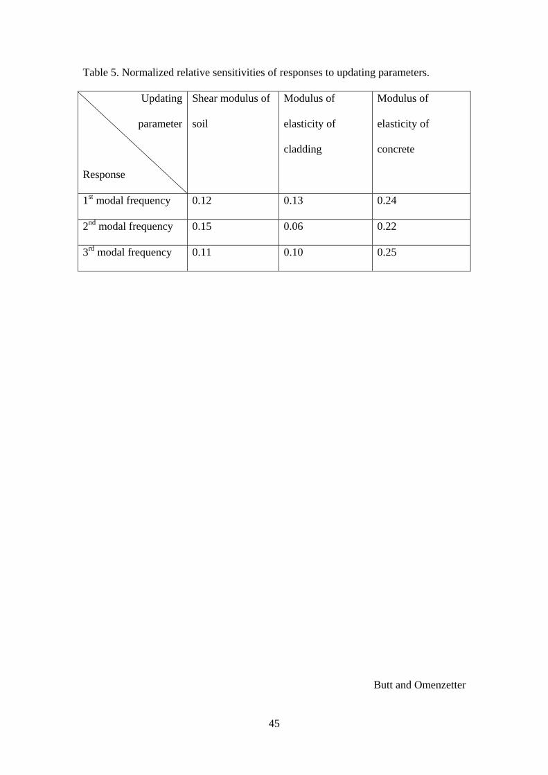
modulus of elasticity of concrete were finally selected. The normalized relative
sensitivities of the target responses to the parameters are shown in Table 5. It can be
observed from the table that the values of the normalized relative sensitivities Snr
considering all the responses show a significant sensitivity for producing a change in
the response. Modulus of elasticity of concrete is the most influential parameter while
the remaining two are almost equally influential but roughly 50% less than the first.
Confidence levels were applied to the updating parameters as the diagonal weighting
matrix Ca entries (Equations (7) and (8)) to take into account uncertainty in their
estimation. For this study, it is assumed that the updating parameters can have a
scatter within ±30%.
Updating results and discussions
FEMtools software (FEMtools 2008) was used in this research for automatic model
updating. In the model updating procedure, error interpreted as an objective function

24
is minimized to improve the response prediction of the model. The following
objective function, representing mean weighted absolute relative frequency error, is
considered in this study:
1 |∆ |100% 10
where n is the total number of target frequencies considered, and and ∆ are the
target frequency and frequency error, respectively, whereas coefficients account
for the estimated relative variabilities of responses.
The automatic iterative procedure for minimizing the objective function is
controlled by a following three convergence criteria:
i) the minimum value of objective function, assumed 0.1%;
ii) the minimum improvement in the objective function between two
consecutive iterations, assumed 0.01%; and
iii) the maximum number of iterations allowed, assumed 50.
The algorithm searching for the global minimum of the objective function may
be lured into local minima instead of the global minimum in problems that Goldberg
et al. (1992) call ‘deceptive’. This undesirable behaviour is well known in the context
of model updating using sensitivity method (Deb 1998). In this study, a two-step
updating strategy was followed to safeguard against being trapped in a local minimum
(Brownjohn and Xia 2000):
Step 1: Starting with the initially assumed values of updating parameters the
objective function is minimized to arrive at an intermediate solution; and
Step 2: The values of the updated parameters obtained in Step 1 were
perturbed by +10%, 0% and -10%, considering all 27 combinations, and the
updating procedure rerun.

25
Results of updating are shown in Table 4. In Step 1, the objective function, ef,
has improved considerably from 6.11% to 0.31%, with the largest individual error not
exceeding 0.33%. While MACs were not explicitly included in the objective function,
improving frequencies typically also improves MACs. This was also the case in the
reported exercise: the MAC values have improved slightly for the first and second
mode and are now equal to 80% and 96%, respectively, while for the third mode
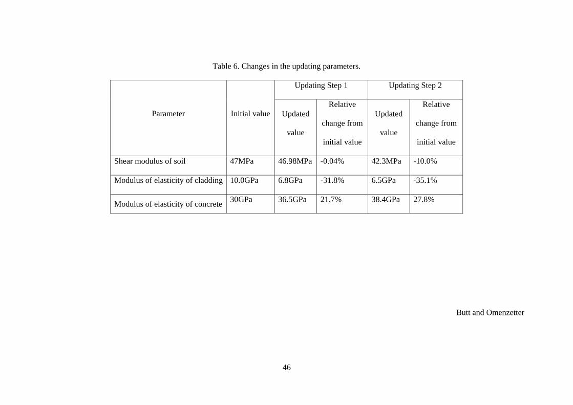
shape it has improved considerably reaching 79%. Table 6 shows the initial and
updated values of stiffness parameters and their relative changes. It can be seen that
the reported changes in modal characteristics were achieved by changing the stiffness
of cladding by -38.1% and 21.7% for concrete, respectively. The soils stiffness
practically did not change (-0.04%).
Due to space limitations, individual results from the 27 runs in Step 2 are not
shown here, however, four clusters of points were discernible. A better solution to that
of Step 1 was found among them, suggesting that Step 1 solution was only a local
minimum and confirming the advantage and need of using the two-step procedure.
Step 2 converged to a very small value of ef=0.03% for the objective function,
providing excellent match of frequencies with the maximum absolute error of 0.07%
(see Table 4), and yielding the final updating parameter values of 42.3MPa for shear
modulus of soil, 6.5GPa for modulus of elasticity of cladding, and 38.4GPa for
modulus of elasticity of concrete (see Table 6). Compared to the initial values the
relative changes were -10.0%, -35.1% and 27.8%, respectively. The shifts in relative
values compared to Step 1 were smaller for cladding and concrete, -3.7% and 6.1%,
and more noticeable, -10.0%, for soil.
Step 2 practically did not change the MACs and their final values are 80%,
96% and 78%. However, improvements in MACs compared to the initial FEM are

26
noticeable. The updated MAC matrix is shown graphically in Figure 5b. The
reduction in the height of the off-diagonal terms is also clear in the figure. Figure 6
shows the comparison between the measured and updated FEM mode shapes at the
roof level assuming the roof to act like a rigid diaphragm. It can be observed from
Figure 6 that the second mode shapes coincide very well, while the first and third
mode shapes are matched reasonably well.
No updating exercise is complete without assessing the plausibility of
numerically obtained results and clear understanding of their limitations. The large
drop in the cladding stiffness (-35.1%) indicates that the assumption of the cladding
being fully fixed to the structural elements was not justified and very likely only
partial fixity exists. Another reason for reduced stiffness are the openings for
windows in the cladding panels which were ignored in the FEM model. Also an initial
overestimation of cladding material modulus of elasticity, taken from literature, is
quite possible. For the modulus of elasticity of concrete the increase is by 27.8%. The
increased value is not outside the typically encountered significant variability of
concrete properties. Also, the initial estimate of modulus of elasticity of RC was
based on typical, conservatively assumed values used in New Zealand building
construction of the era but the exact design or laboratory tested values were unknown.
For those reasons, the updated value is not unreasonable. It is also possible that other
non-structural elements, whose stiffness was not updated, could have made a
contribution towards larger stiffness. One would expect more uncertainty in the soils
properties, but, perhaps unexpectedly, the change in the soil shear modulus after
updating was only -10.0%. This was rather due to luck in the initial estimate than
anything else. For all the parameters it needs to be emphasized that they are the global
stiffness of soil, concrete and cladding without taking into account any possible local

27
spatial variations. In general, the updated model represents the optimal solution for
the frequency matching problem of Equation (10) that is also justified by engineering
judgment, but hinges on the validity of the initial model topology, discretization and
parameterization. We argue though that these are adequate.
Validation of the updated model
To further validate the updated FEM, the simulated response is compared with the
recorded response of the earthquake of October 10th, 2009, that produced the largest
PGAs and PRAs at the building site. The updated FEM was exported to ABAQUS
from FEMtools to perform time history analysis. For time history analysis, all three
directions of the acceleration record measured at the base level at sensor 6 were
applied simultaneously at all the column foundations in agreement with the fact that
there are tie-beams linking all the foundations and that the measured accelerations at
the base level at sensor 6 and 7 were the same for practical reasons. A constant
damping of 5% was considered for all the modes as recommended by NZS 1170.5
(Standards New Zealand 2004) for time history analysis for serviceability limit state.
(This code recommended damping ratio was used rather than the identified values due
to considerable spread of the latter as mentioned earlier. Table 4 shows that the
measured values were not significantly different than 5% either.)
To quantify the improvement in response prediction due to updating the
following relative error measures were adopted (Sprague and Geers 2004):
∑∑
1 11
1cos
∑
∑ ∑ 12
28
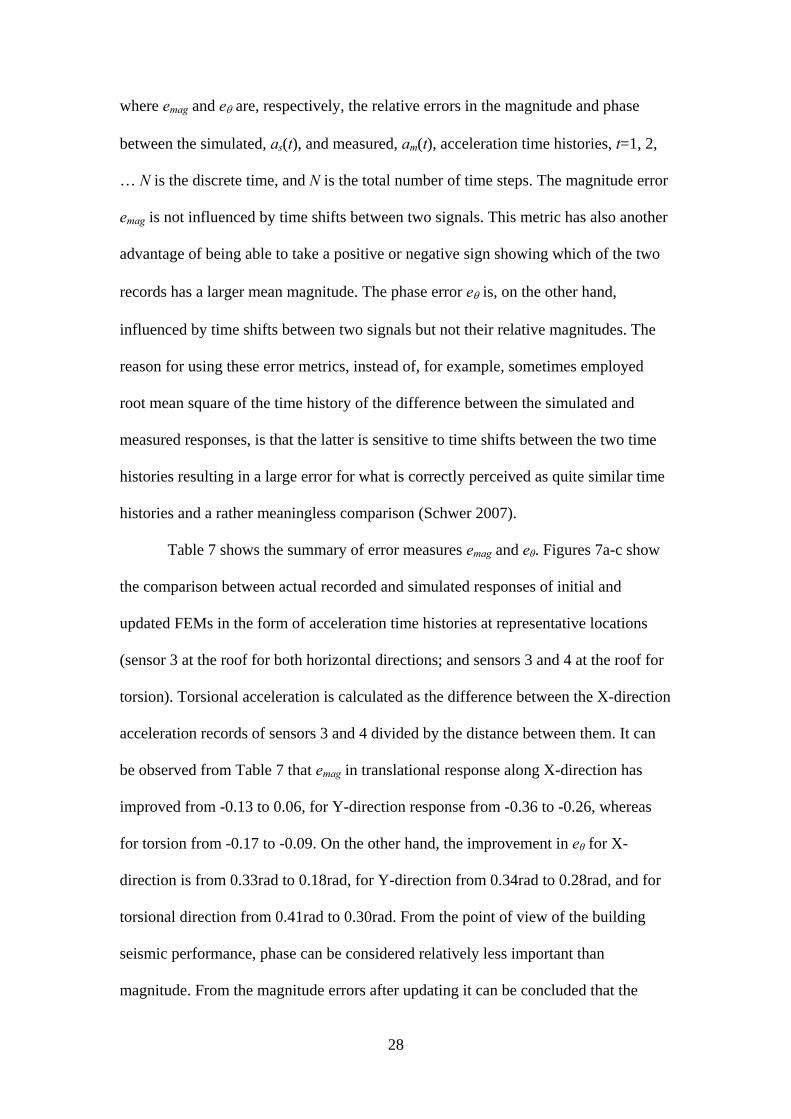
where emag and e are, respectively, the relative errors in the magnitude and phase
between the simulated, as(t), and measured, am(t), acceleration time histories, t=1, 2,
… N is the discrete time, and N is the total number of time steps. The magnitude error
emag is not influenced by time shifts between two signals. This metric has also another
advantage of being able to take a positive or negative sign showing which of the two
records has a larger mean magnitude. The phase error e is, on the other hand,
influenced by time shifts between two signals but not their relative magnitudes. The
reason for using these error metrics, instead of, for example, sometimes employed
root mean square of the time history of the difference between the simulated and
measured responses, is that the latter is sensitive to time shifts between the two time
histories resulting in a large error for what is correctly perceived as quite similar time
histories and a rather meaningless comparison (Schwer 2007).
Table 7 shows the summary of error measures emag and eθ. Figures 7a-c show
the comparison between actual recorded and simulated responses of initial and
updated FEMs in the form of acceleration time histories at representative locations
(sensor 3 at the roof for both horizontal directions; and sensors 3 and 4 at the roof for
torsion). Torsional acceleration is calculated as the difference between the X-direction
acceleration records of sensors 3 and 4 divided by the distance between them. It can
be observed from Table 7 that emag in translational response along X-direction has
improved from -0.13 to 0.06, for Y-direction response from -0.36 to -0.26, whereas
for torsion from -0.17 to -0.09. On the other hand, the improvement in eθ for X-
direction is from 0.33rad to 0.18rad, for Y-direction from 0.34rad to 0.28rad, and for
torsional direction from 0.41rad to 0.30rad. From the point of view of the building
seismic performance, phase can be considered relatively less important than
magnitude. From the magnitude errors after updating it can be concluded that the

29
agreement of simulated and measured responses along X- and torsional directions has
improved markedly and is now very close, whereas along Y-direction, despite some
improvement, more noticeable difference is still present. The phase errors also
decreased and are now between 0.18rad and 0.30rad.
Assessment of serviceability limit state performance using initial and updated
FEM
Under the serviceability limit state, the building response should remain
predominantly elastic and avoidance of excessive lateral deformations to prevent non-
structural damage is the primary control parameter. The inter-story drift ratio, defined
as the relative displacement between the top and bottom of the story divided by story
height, is commonly assumed to control the onset of non-structural damage
(Dymiotis-Wellington and Vlachaki 2004). Therefore, to study the serviceability limit
state performance of the building, the maximum inter-story drift ratios for a random
selection of 10 seismic events recorded at the building site (see Table 8) and
appropriately scaled were calculated. For the purpose of comparison, the analysis is
performed for both the initial and updated FEMs.
All the available earthquakes recorded at the building site are of low intensity,
it is therefore necessary to scale those to the serviceability limit state level shaking.
The scaling procedure recommended in the NZS 1170.5 (Standards New Zealand
2004) was followed for the selected 10 earthquakes. In short, it requires minimizing
the logarithmic root-mean-square difference between the actual and target spectra in a
frequency range encompassing the fundamental frequency of the structure at hand.
The assumed target code spectrum for a return period of 25 years and hazard factor of
0.4 is shown in Figures 8a and b along with the spectra of the 10 earthquakes for both
X- and Y-direction components, respectively. The scaling factors for the selected 10

30
events to match the target spectrum are reported in Table 8; they range between 17
and 676. Since the measured X- and Y- components of the records were different, the
scaling factors for both orthogonal components are also different. The period range
for spectrum matching was between 0.13sec and 0.43sec (2.32Hz and 7.69Hz).
For calculating inter-story drift ratios, the scaled X- and Y-direction
components of a record were applied simultaneously to run the time history analysis
for both initial and updated FEMs. As previously, when validating the updated FEM,
a constant damping of 5% was considered for all the modes. The lateral displacements
along X- and Y-directions at the four corners of each floor level were determined,
inter-story drift ratios corresponding to the two directions calculated separately, and
maximum ratios selected. For all the considered excitation cases, the largest inter-
story drift ratios were observed between the first and the ground floor. Table 8 shows
the maximum inter-story drift ratios for the considered 10 earthquakes for both initial
and updated FEMs along X- and Y-directions. The values for X-direction are between
0.06% and 0.16% and between 0.07% and 0.21% for the initial and updated model,
respectively; for Y-direction these ranges are between 0.06% and 0.13% and between
0.07% and 0.15%, respectively. It can be observed that the updated FEM provides
larger inter-story drift ratios, by 31% and 25% for the X- and Y-direction,
respectively, than the initial FEM. This is because it is less stiff as evident from the
modal frequencies, however, since the relative increase varies between the
earthquakes matching of building resonant frequencies and spectral content of
excitation play a role too.
The recommended limiting inter-story drift ratios reported in the literature and
recommended by various codes vary widely between 0.06% and 0.6% (Bertero et al.
1991). Dymiotis-Wellington and Vlachaki (2004) recommend 0.2% as the critical

31
inter-story drift ratio based on their observations on RC buildings. They argued that
higher limiting values can cause significant yielding in the structure and correspond to
a damage state beyond serviceability. Taking this latter limit value, it can be
concluded that for the considered scaled seismic events, the building has reached or
just exceeded the serviceability limit state of 0.2% inter-story drift for two events,
EQ1 and EQ8, for the updated FEM (Table 8). Overall, the serviceability performance
can be judged as satisfactory. However, the initial FEM produced unconservative,
lower values. This confirms the benefit and importance of using a calibrated structural
model in checking performance criteria.
Finally, since linear FEMs were used in the serviceability study, it is in order
to assess if the linearity assumption is justified. The maximum inter-story drift ratio
reported in Table 8 is 0.21%, with the majority of values noticeably lower.
Insufficient information is available (such as the exact reinforcement ratios and
detailing, or on nonlinear behaviour of cladding and its connections to the RC frame)
that would enable the creation of a detailed and realistic nonlinear FEM to be
subjected to time history analysis to see if it enters nonlinear range at the
serviceability level response. However, some indirect inferences can be made.
Serviceability limit state can be understood as separating the linear and nonlinear
structural behaviour (Dymiotis-Wellington and Vlachaki 2004). Mosalam et al.
(1997) considers it to be limited to the case of insignificant damage where repair is
only required to non-structural elements, and gives the critical inter-story drift ratio in
the range between 0.2% and 0.5%. Eurocode 8 (European Committee for
Standardisation (2003) also implies avoidance of damage and gives similar limits for
the inter-storey drift ratios for damage in non-structural elements between 0.2% and
0.5%. As far as yielding in structural elements is concerned, a study by Dymiotis-

32
Wellington and Vlachaki (2004) showed, despite its limited scope, that inter-story
drifts of 0.2% resulted in mild yielding (rotational ductility less than 2) in only some
beams of an RC frame designed to Eurocode 8. As in our study the maximum inter-
story drift ratio is 0.21%, with the majority of remaining values noticeably lower,
there are good reasons to believe that the building will experience at most only mild
nonlinear responses and the linear FEM used were able to predict its serviceability
limit state behaviour reasonably well.
Conclusions
This study was concerned with seismic response of an instrumented three story RC
building. The first part focused on review of modal properties identified using 50
seismic response records. The records, varying in amplitude, enabled determination of
trends in frequencies with increasing amplitude of response. The frequencies showed
a clear decreasing trend with increasing PRA, which could be reasonably represented
by a linear relationship. The identified damping ratios, however, had scattered values
with no clear trend.
The second part was concerned with numerical modelling of the building and
its seismic responses. As series of FEMs including SSI and NSCs was first developed
and the influence of different structural and non-structural components, and the effect
of soil on the building dynamics analysed. It was found that NSCs and SSI contribute
significantly to modal dynamic response and these should be included in FEMs to
replicate the true in-situ behaviour. The final FEM produced resonance frequencies
within 7.5% of those identified experimentally. The final FEM was further improved
using a sensitivity based model updating technique. The updating parameters included
a structural parameter (stiffness of concrete), a non-structural parameter (stiffness of
cladding), and soil stiffness. The match between the frequencies after updating was
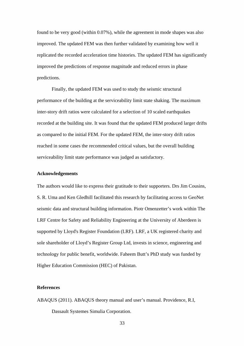
33
found to be very good (within 0.07%), while the agreement in mode shapes was also
improved. The updated FEM was then further validated by examining how well it
replicated the recorded acceleration time histories. The updated FEM has significantly
improved the predictions of response magnitude and reduced errors in phase
predictions.
Finally, the updated FEM was used to study the seismic structural
performance of the building at the serviceability limit state shaking. The maximum
inter-story drift ratios were calculated for a selection of 10 scaled earthquakes
recorded at the building site. It was found that the updated FEM produced larger drifts
as compared to the initial FEM. For the updated FEM, the inter-story drift ratios
reached in some cases the recommended critical values, but the overall building
serviceability limit state performance was judged as satisfactory.
Acknowledgements
The authors would like to express their gratitude to their supporters. Drs Jim Cousins,
S. R. Uma and Ken Gledhill facilitated this research by facilitating access to GeoNet
seismic data and structural building information. Piotr Omenzetter’s work within The
LRF Centre for Safety and Reliability Engineering at the University of Aberdeen is
supported by Lloyd's Register Foundation (LRF). LRF, a UK registered charity and
sole shareholder of Lloyd’s Register Group Ltd, invests in science, engineering and
technology for public benefit, worldwide. Faheem Butt’s PhD study was funded by
Higher Education Commission (HEC) of Pakistan.
References
ABAQUS (2011). ABAQUS theory manual and user’s manual. Providence, R.I,
Dassault Systemes Simulia Corporation.

34
ASCE/SEI 7-05 (2005). Minimum design loads for buildings and other structures.
Reston, VA, Structural Engineering Institute of the American Society of Civil
Engineers.
Bertero, V. V., Anderson, J. C., Krawinkler, H., Miranda, E. and the CURE and
Kajima Research Teams (1991). Design guidelines for ductility and drift
limits: Review of state-of-the-art in ductility and drift-based earthquake
resistant design of buildings. UCB/EERC 91/15, Berkeley, CA, The
University of California.
Berto, L. R., Vitaliani, A., Saetta, A. and Simioni, P. (2009). "Seismic assessment of
existing RC structures affected by degradation phenomena." Structural Safety
31(4): 284-297.
Bhattacharya, K. and Dutta, S. C. (2004). "Assessing lateral period of building frames
incorporating soil flexibility." Journal of Sound and Vibration 269(3-5): 795-
821.
Bodeux, J. B. and Golinval, J. C. (2001). "Application of ARMAV models to the
identification and damage detection of mechanical and civil engineering
structures." Smart Materials and Structures, 10: 479-489.
Boon, D., Perrin, N. D., Dellow, G. D., Van Dissen, R. and Lukovic, B. (2011).
"NZS1170.5:2004 site subsoil classification of Lower Hutt." Proceedings of
the 2011 Pacific Conference on Earthquake Engineering, Auckland: 1-8.
Bowles, J. E. (1996). Foundation analysis and design. Singapore, McGraw-Hill.
Brownjohn, J. M. W., Hong, H. and Chien, P. T. (2001a). Assessment of structural
condition of bridges by dynamic measurements. Singapore, Nanyang
Technological University.

35
Brownjohn, J. M. W., Moyo, P., Omenzetter, P., and Lu, Y. (2003). "Assessment of
highway bridge upgrading by dynamic testing and finite-element model
updating." Journal of Bridge Engineering, ASCE 8(3): 162-172.
Brownjohn, J. M. W. and Xia, P. Q. (2000). "Dynamic assessment of curved cable-
stayed bridge by model updating." Journal of Structural Engineering, ASCE
126(2): 252-260.
Brownjohn, J. M. W., Xia, P. Q., Hao, H., and Xia, Y. (2001b). "Civil structure
condition assessment by FE model updating: Methodology and case studies."
Finite Elements in Analysis and Design 37(10): 761-775.
Butt, F. and Omenzetter, P. (2012).”Evaluation of seismic response trends from long-
term monitoring of two instrumented RC buildings including soil-structure
interaction.” Advances in Civil Engineering 2012:1-18.
Celebi, M. (2006). "Recorded earthquake responses from the integrated seismic
monitoring network of the Atwood building, Anchorage, Alaska." Earthquake
Spectra 22(4): 847-864.
Celebi, M. and Safak, E. (1991). "Seismic response of Transamerica building. I: Data
and preliminary analysis." Journal of Structural Engineering, ASCE 117(8):
2389-2404.
Celebi, M. and Safak, E. (1992). "Seismic response of Pacific Park Plaza. I: Data and
preliminary analysis." Journal of Structural Engineering, ASCE 118(6): 1547-
1565.
European Committee for Standardisation (2003). Eurocode 8: Design of structures for
earthquake resistance - Part 1: General rules, seismic actions and rules for
buildings. Brussels, European Committee for Standardisation.

36
Dascotte, E., Strobbe, J. and Hua, H. (1995). "Sensitivity based model updating using
multiple types of simultaneous state variables." Proceedings of the 13th
International Modal Analysis Conference. Bethel, MN: 1-6.
Deb, K. (1998). Optimization for engineering design: algorithms and examples. New
Delhi, Prentice-Hall of India.
Dymiotis-Wellington, C. and Vlachaki, C. (2004). "Serviceability limit state criteria
for the seismic assessment of RC buildings." Proceedings of the 13th World
Conference on Earthquake Engineering. Vancouver, BC: 1-10.
Ewins, D. J. (2000). Modal testing: Theory, practice and application. Baldock,
Research Studies Press.
FEMtools (2008). FEMtools model updating theoretical manual and user's manual.
Leuven, Dynamic Design Solutions.
Foti, D., Diaferio, M., Giannoccaro, N. I. and Mongelli, M. (2012). “Ambient
vibration testing, dynamic identification and model updating of a historic
tower.” Nondestructive Testing and Evaluation International 47: 88-95.
Friswell, M. I. and Mottershead, J. E. (1996). Finite element model updating in
structural dynamics. Dordrecht, Netherlands, Kluwer Academic Publishers.
Gaylord, M. W. (1974). Reinforced plastics: Theory and practice. New York, NY,
Cahners.
Gazetas, G. (1991). "Formulas and charts for impedances of surface and embedded
foundations." Journal of Geotechnical Engineering, ASCE 117(9): 1363-1381.
GeoNet (2013). Structural array data.
http://info.geonet.org.nz/display/appdata/Structural+Array+Data, accessed 30
July 2013.

37
Geers, T. L. (1984). "An objective error measure for the comparison of calculated and
measured transient response histories." The Shock and Vibration Bulletin
54(2): 99-107.
Goldberg, D. E., Deb, K. and Horn, J. (1992). Massive multimodality, deception, and
genetic algorithms, Parallel Problem Solving from Nature 2: 37-46.
Hart, G. C. and Yao, J. T. P. (1976). "System identification in structural dynamics."
Journal of Engineering Mechanics, ASCE 103(6): 1089–1104.
Kanvinde, A. M., and Deierlein, G. G. (2006). "Analytical models for the seismic
performance of gypsum drywall partitions." Earthquake Spectra 22(2): 391-
411.
Lee, T. H., Kato, M., Matsumiya, T., Suita, K. and Nakashima, M. (2007). "Seismic
performance evaluation of non-structural components: Drywall partitions."
Earthquake Engineering and Structural Dynamics 36(3): 367-382.
Lin, C. C., Wang, J. F. and Tsai, C. H. (2008). "Dynamic parameter identification for
irregular buildings considering soil-structure interaction effects." Earthquake
Spectra 24(3): 641-666.
Montgomery, D., Peck, E. A. and Vining, G. (2001). Introduction to linear regression
analysis. New York, NY, Wiley.
Mosalam K. M., Ayala G., White R. N. and Roth C. (1997). "Seismic reliability of
LRC frames with and without masonry infill walls." Journal of Earthquake
Engineering, ASCE, 1(4): 693-720.
Mulliken, J. S. and Karabalis, D. L. (1998). "Discrete model for dynamic through-the-
soil coupling of 3-D foundations and structures." Earthquake Engineering and
Structural Dynamics 27(7): 687-710.

38
Pan, T. C., You, X. and Brownjohn, J. M. W. (2006). "Effects of infill walls and floor
diaphragms on the dynamic characteristics of a narrow-rectangle building."
Earthquake Engineering and Structural Dynamics 35(5): 637-651.
Safak, E. (1993). "Response of a 42-storey steel-frame building to the MS=7.1 Loma
Prieta earthquake." Engineering Structures 15(6): 403-421.
Saito, T. and Yokota, H. (1996). "Evaluation of dynamic characteristics of high-rise
buildings using system identification techniques." Journal of Wind
Engineering and Industrial Aerodynamics 59(2-3): 299-307.
Satake, N. and Yokota, H. (1996). "Evaluation of vibration properties of high-rise
steel buildings using data of vibration tests and earthquake observations."
Journal of Wind Engineering and Industrial Aerodynamics 59(2-3): 265-282.
Schwer, L. E. (2007). "Validation metrics for response histories: Perspectives and
case studies." Engineering with Computers 23: 295-309.
Shakib, H. and Fuladgar, A. (2004). "Dynamic soil-structure interaction effects on the
seismic response of asymmetric buildings." Soil Dynamics and Earthquake
Engineering 24(5): 379-388.
Sohn, H., Farrar, C. R., Hemez, F. M., Shunk, D. D., Stinemates, D. W. and Nadler,
B. R. (2003). A review of structural health monitoring literature: 1996–2001.
Los Alamos, NM, Los Alamos National Laboratory.
Sprague, M. A. and Geers, T. L. (2004). "A spectral-element method for modelling
cavitation in transient fluid-structure interaction." International Journal for
Numerical Methods in Engineering 60(15): 2467-2499.
Standards New Zealand (2004). NZS 1170.5:2004. Structural design actions. Part 5:
Earthquake actions – New Zealand. Wellington, Standards New Zealand.

39
Steel, R. and Torrie, J. (1960). Principles and procedures of statistics. New York, NY,
McGraw-Hill.
Stewart, J. P. and Fenves, G. L. (1998). "System identification for evaluating soil-
structure interaction effects in buildings from strong motion recordings."
Earthquake Engineering and Structural Dynamics 27(8): 869-885.
Su, R. K. L., Chandler, A. M., Sheikh, M. N. and Lam, N. T. K. (2005). "Influence of
non-structural components on lateral stiffness of tall buildings." Structural
Design of Tall and Special Buildings 14(2): 143-164.
Titurus, B. and Friswell, M. I. (2008). "Regularization in model updating."
International Journal for Numerical Methods in Engineering 75: 440-478.
Trifunac, M. D., Ivanovic, S. S. and Todorovska, M. I. (2001). "Apparent periods of a
building. I: Fourier analysis." Journal of Structural Engineering, ASCE
127(5): 517-526.
Trifunac, M. D. and Todorovska, M. I. (1999). “Recording and interpreting
earthquake response of full-scale structures.” Proceedings of the NATO
Advanced Research Workshop on Strong-Motion Instrumentation for Civil
Engineering Structures. Dordrecht, Kluwer: 131-155.
Uma, S. R., Zhao, J. X. and King, A. B. (2010). "Seismic actions on acceleration
sensitive non-structural components in ductile frames." Bulletin of the New
Zealand Society for Earthquake Engineering 43(2): 110-125.
Van Overschee, P. and De Moor, B. (1994). "N4SID: Subspace algorithms for the
identification of combined deterministic-stochastic systems." Automatica
30(1): 75-93.

40
Wang, H., Li, A. and Li, J. (2010). "Progressive finite element model calibration of a
long-span suspension bridge based on ambient vibration and static
measurements." Engineering Structures 32(9): 2546-2556.
Weng, J.-H., Loh, C.-H. and Yang, J. N. (2009). "Experimental study of damage
detection by data-driven subspace identification and finite element model
updating.” Journal of Structural Engineering, ASCE 135(12): 1533-1544.
Wu, J. R. and Li, Q. S. (2004). “Finite element model updating for a high-rise
structure based on ambient vibration measurements.” Engineering Structures
26(7): 979-990.
Zhang, Q. W., Chang, C. C. and Chang, T. Y. P. (2000). "Finite element model
updating for structures with parametric constraints." Earthquake Engineering
and Structural Dynamics, 29(7): 927-944.

41
Table 1. Maximum PGA and PRA recorded by individual sensors.
Sensor Max. acceleration in X-direction
(g)
Max. acceleration in Y-direction
(g)
Free field
10 (PGA) 0.0074 0.0138
Foundation
6 (PGA) 0.0059 0.0092
7 (PGA) 0.0061 0.0090
Roof
3 (PRA) 0.0185 0.0390
4 (PRA) 0.0206 0.0412
Butt and Omenzetter

42
Table 2. Summary of identified frequencies and damping ratios for flexible base model.
Mode
Frequency Damping ratio
Min.
(Hz)
Max.
(Hz)
Avg.
(Hz)
Relative
spread
(%)
Min.
(%)
Max.
(%)
Avg.
(%)
Relative
spread
(%)
1st 3.04 3.50 3.33 14 1.2 7.3 3.4 176
2nd 3.21 3.88 3.61 19 1.4 12.1 5.6 190
3rd 3.48 3.90 3.79 11 1.0 8.3 3.1 240
Butt and Omenzetter

43
Table 3. Comparison of results of different stages of FEM modal analysis with
measured values.
Mode
Frequencies
(Hz)
Stage I Stage II Stage III Stage IV Stage V Stage VI Measured
value
1st
2.12
(-30.3%)
2.20
(-27.6%)
2.43
(-20.1%)
2.98
(-2.0%)
2.58
(-15.1%)
2.91
(-4.3%) 3.04
2nd 2.45
(-23.7%)
2.50
(-22.1%)
3.24
(1.0%)
3.96
(23.4%)
3.11
(-3.1%)
3.45
(7.5%) 3.21
3rd 2.30
(-34.0%)
2.41
(-30.8%)
3.00
(-13.8%)
3.67
(5.5%)
3.19
(-8.3%)
3.68
(5.8%) 3.48
Note: The values in parenthesis show the percentage difference between the particular
FEM stage and measured values.
Butt and Omenzetter

44
Table 4. Correlation between initial and updated FEMs and measured response of October 10th, 2009.
Mode Measured responses FEM frequencies
(Hz)
Difference between FEM and
measured frequencies
(%)
MAC
(%)
Frequency
(Hz)
Damping
ratio
(%)
Initial
model
Updating
Step 1
Updating
Step 2
Initial
model
Updating
Step 1
Updating
Step 2
Initial
model
Updating
Step 1
Updating
Step 2
1st 3.04 4.7 2.92 3.03 3.038 -3.95 -0.33 -0.07 78 80 80
2nd 3.21 4.6 3.45 3.20 3.21 7.48 -0.31 0.00 92 96 96
3rd 3.48 3.6 3.72 3.49 3.479 6.90 0.29 -0.03 63 79 78
Objective function ef 6.11 0.31 0.03
Butt and Omenzetter
45
Table 5. Normalized relative sensitivities of responses to updating parameters.
Updating
parameter
Response
Shear modulus of
soil
Modulus of
elasticity of
cladding
Modulus of
elasticity of
concrete
1st modal frequency 0.12 0.13 0.24
2nd modal frequency 0.15 0.06 0.22
3rd modal frequency 0.11 0.10 0.25
Butt and Omenzetter
46
Table 6. Changes in the updating parameters.
Parameter Initial value
Updating Step 1 Updating Step 2
Updated
value
Relative
change from
initial value
Updated
value
Relative
change from
initial value
Shear modulus of soil 47MPa 46.98MPa -0.04% 42.3MPa -10.0%
Modulus of elasticity of cladding 10.0GPa 6.8GPa -31.8% 6.5GPa -35.1%
Modulus of elasticity of concrete30GPa 36.5GPa 21.7% 38.4GPa 27.8%
Butt and Omenzetter

47
Table 7. Magnitude and phase errors in response time histories for initial and updated models
Direction X Y Torsional
FEM Initial Updated Initial Updated Initial Updated
emag (-) -0.13 0.06 -0.36 -0.26 -0.17 -0.09
eθ (rad) 0.33 0.18 0.34 0.28 0.41 0.30
Butt and Omenzetter

48
Table 8. Earthquake records used in serviceability study, scaling factors and maximum inter-story drift ratios Earthquake
designation
Date
(DD/MM/YYYY) and
time of occurrence
(GMT)
PGA recorded at
sensor 6 (g)
Scaling factor Maximum inte
X-
direction
Y-
direction
X-
direction
Y-
direction
X-direction
Initial
FEM
U
F
EQ1 09/06/2008, 02:58 0.0016 0.0013 74 82 0.12 0
EQ2 09/14/2008, 09:25 0.0014 0.0018 81 65 0.13 0
EQ3 10/17/2008, 00:25 0.0003 0.0004 676 443 0.10 0
EQ4 12/26/2008, 19:49 0.0032 0.0032 35 33 0.06 0
EQ5 05/01/2009, 05:16 0.0036 0.0022 52 64 0.09 0
EQ6 08/05/2009, 17:51 0.0010 0.0016 123 71 0.07 0
EQ7 10/10/2009, 05:02 0.0059 0.0092 22 17 0.09 0
EQ8 11/18/2009, 1804 0.0022 0.0025 41 42 0.16 0
EQ9 12/08/2009, 22:09 0.0018 0.0018 78 67 0.07 0
EQ10 02/12/2010, 13:41 0.0034 0.0029 34 41 0.08 0
Butt and Omenzetter

1
a)
b)
Figure 1. Instrumented RC building: a) typical floor plan showing general dimensions
and location of stairs and elevator shaft, and b) 3D view of the building and sensor
array.
Butt and Omenzetter

2
Figure 2. Inputs and outputs for evaluating SSI effects in system identification of
buildings (Stewart and Fenves 1998).
Butt and Omenzetter
Roof: ug+uf+hθ+u
h
Free field: ug
Foundation rocking: θ Foundation translation: ug +uf
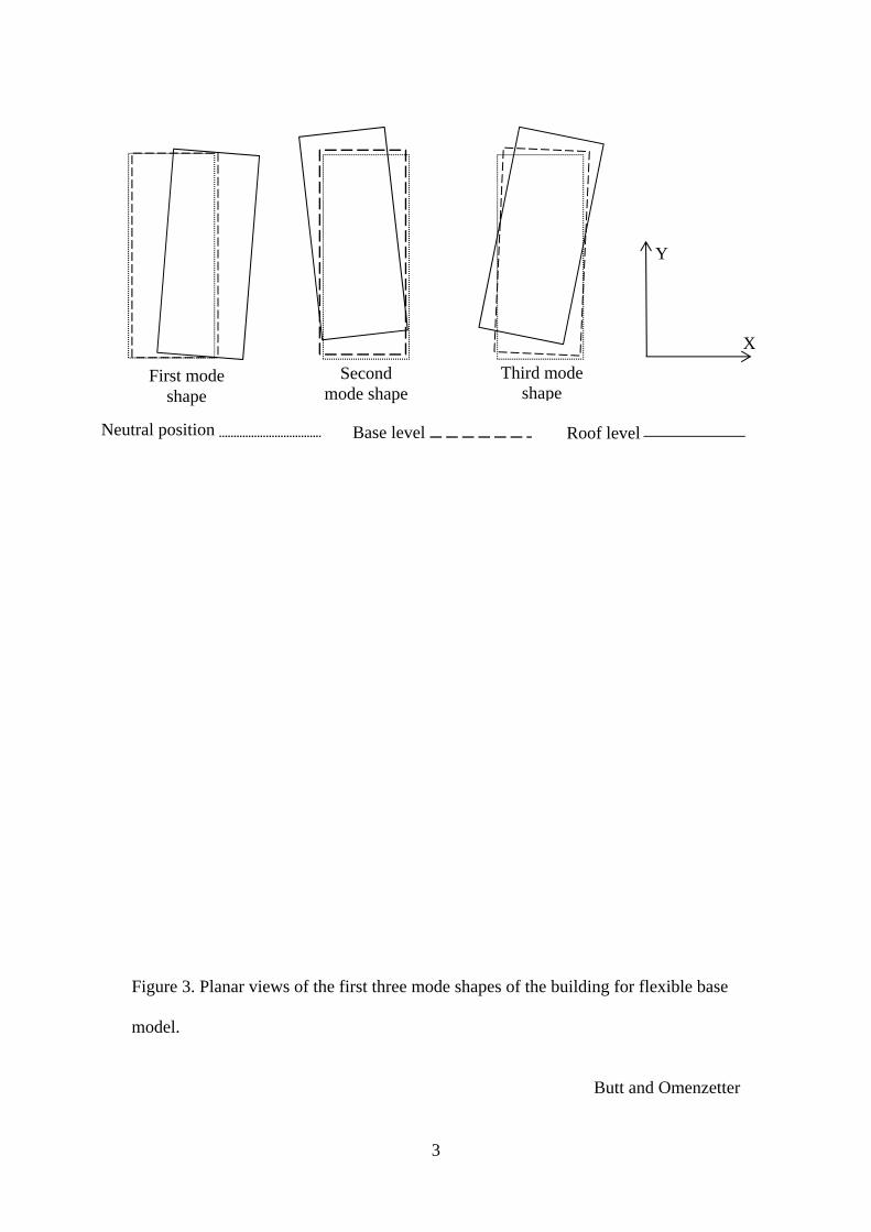
3
Figure 3. Planar views of the first three mode shapes of the building for flexible base
model.
Butt and Omenzetter
Y
First mode shape
Second mode shape
Third mode shape
X
Neutral position Base level Roof level

4
a)
b)
Figure 4. First three modal frequencies of the building for flexible base case vs. PRA of sensor 3: a) X-direction, and b) Y-direction.
Butt and Omenzetter

5
a)
b)
Figure 5. MAC matrix between FEM and measured mode shapes: a) initial FEM, and
b) updated FEM.
Butt and Omenzetter

6
Figure 6. Comparison between mode shapes of the updated FEM and measured
response at the roof level.
Butt and Omenzetter
Neutral position Updated FEM Measured
First mode shape
Second mode
shape
Third mode shape

7
a)
b)
Figure 7. Recorded and simulated acceleration time histories using initial and updated
FEMs at the roof for the October 10th, 2009 earthquake: a) X-direction, b) Y-
direction, and c) torsion.
Butt and Omenzetter

8
c)
Figure 7. Recorded and simulated acceleration time histories using initial and updated
FEMs at the roof for the October 10th, 2009 earthquake: a) X-direction, b) Y-
direction, and c) torsion.
Butt and Omenzetter

9
a)
Figure 8. Target ground motion spectrum from NZS 1170.5:2004 and scaled spectra
for 10 seismic events used in serviceability study: a) X-direction, and b) Y-direction.
Butt and Omenzetter

10
b)
Figure 8. Target ground motion spectrum from NZS 1170.5:2004 and scaled spectra
for 10 seismic events used in serviceability study: a) X-direction, and b) Y-direction.
Butt and Omenzetter


