
ECONOMIC ANALYSIS GROUPDISCUSSION PAPER
Search, Price Dispersion, and Local Competition: Estimating Heterogeneous Search Costsin Retail Gasoline Markets
by
Mitsukuni Nishida and Marc Remer*EAG 14-2 July 2014
EAG Discussion Papers are the primary vehicle used to disseminate research from economists in theEconomic Analysis Group (EAG) of the Antitrust Division. These papers are intended to informinterested individuals and institutions of EAG’s research program and to stimulate comment andcriticism on economic issues related to antitrust policy and regulation. The Antitrust Divisionencourages independent research by its economists. The views expressed herein are entirely thoseof the author and are not purported to reflect those of the United States Department of Justice.
Information on the EAG research program and discussion paper series may be obtained from RussellPittman, Director of Economic Research, Economic Analysis Group, Antitrust Division, U.S. De-partment of Justice, LSB 9004, Washington, DC 20530, or by e-mail at [email protected] on specific papers may be addressed directly to the authors at the same mailing addressor at their e-mail addresses.
To obtain a complete list of titles or to request single copies of individual papers, please write toKathy Burt at [email protected] or call (202) 307-5794. In addition, recent papers are nowavailable on the Department of Justice website at http://www.justice.gov/atr/public/eag/discussion-papers.html.
*Mitsukuni Nishida: The Johns Hopkins Carey Business School, 100 International Drive Baltimore, MD 21202. Email:[email protected]. Marc Remer: Economic Analysis Group, U.S. Department of Justice. Email: [email protected]. Theviews expressed in this article are entirely those of the author and are not purported to reflect those of the U.S. Department ofJustice. We have benefited from discussions with Maqbool Dada, Babur De Los Santos, Emin M. Dinlersoz, Elisabeth Honka,Han Hong, Ali Hortacsu, Sergei Koulayev, Jose Luis Moraga-Gonzalez, Aviv Nevo, Zsolt Sandor, Stephan Seiler, Chad Syverson,Matthijs Wildenbeest, Xiaoyong Zheng, and seminar participants at North Carolina State University, Kyoto University, JohnsHopkins University, University of Tokyo, Center for Economic Studies at US Census Bureau, 2013 IIOC, and the 5th workshopon consumer search and switching costs. We thank Reid Baughman, Autumn Chen, Yajing Jiang, Sam Larson, Jianhui Li, andKarry Lu for research assistance. The retail gasoline price data for this project were generously provided by Mariano Tappata.

Abstract
Information frictions play a key role in a wide array of economic environments andare frequently incorporated into formal models as search costs. Yet, as search costs aretypically unobserved, little empirical work investigates the determinants of the distri-bution of consumer search costs and the implications for policy. This paper exploresthe sources of heterogeneity in consumer search costs and how this heterogeneity andmarket structure shape firms’ equilibrium pricing and consumers’ search behavior inretail gasoline markets. We estimate the distribution of consumer search costs usingprice data for a large number of geographically isolated markets across the UnitedStates. The results demonstrate that the distribution of consumer search costs variessignificantly across geographic markets and that market and population characteristics,such as household income, explain some of the variation. Policy counterfactuals suggestthat the shape of the consumer search cost distribution has important implications forboth government policy and firms’ strategic pricing behavior. The experiments revealthat (1) the search cost distribution needs to be sufficiently heterogeneous to generateequilibrium price dispersion, and (2) the market-level expected price paid decreases inthe number of firms, but consumers with high search costs may be worse off from anincreased number of firms.

1 Introduction
Information frictions play a key role in explaining many aspects of economic activity. For instance,
a robust body of economic research has identified and explained the existence of price dispersion in
both homogeneous and differentiated product markets as a consequence of consumer search costs.
Since Stigler’s (1961) seminal article, a number of influential theoretical papers, such as Varian
(1980), Burdett and Judd (1983), and Stahl (1989), demonstrate that information frictions resulting
from consumer search costs can lead to competing firms setting different prices for homogeneous
goods.1 Search costs have also played an important role in characterizing labor and monetary
markets.2
Although search costs are an important component of many theoretical models, we know very
little about what determines consumers’ search cost distributions and its implications for policy
and pricing as search costs are typically unobserved. For instance, there exists little empirical work
that documents how and why consumer search costs vary across geographic markets. This gap in
the literature is unfortunate because measuring and understanding the source of variation in search
costs can benefit government policy and help understand firms’ pricing strategy, which critically
depends upon both market structure and the distribution of consumer search costs in a market. For
instance, as we later show, a policy or technological improvement that lowers the average cost of
search, but also reduces the variance of the search cost distribution, can lead to higher equilibrium
prices.
This paper fills this gap by exploring the determinants of consumer search costs and their role
in shaping equilibrium pricing and search behavior. To do so, we first structurally estimate the
search cost distributions for each of many retail gasoline geographic markets. We document that
search costs vary considerably both within and across markets. As detailed below, the shape of the
consumer search cost distribution has important implications for both government policy and firms’
strategic pricing behavior. In our counterfactual policy experiments, we find that (1) the search
cost distribution needs to be sufficiently heterogeneous to generate equilibrium price dispersion,
and (2) the market-level expected price paid decreases in the number of firms, but consumers with
high search costs may be worse off from an increased number of firms.3
1See Baye, Morgan, and Scholten (2006) for a broad review of the consumer search and price dispersion literature.2For reviews of search-theoretic models in labor economics, see Rogerson, Shimer, and Wright (2005) and Eckstein
and Van den Berg (2007). For reviews in monetary economics, see Rupert, Schindler, Shevchenko, and Wright (2000).3We use the terms “gas station” and “firm” interchangeably.
2

We proceed in two steps. First, the extent to which consumers’ search costs vary across geo-
graphic markets is explored. Instead of relying on indirect measures of search behavior, such as
internet usage for searching for online insurance products (Brown and Goolsbee 2002), we lever-
age the non-sequential search model developed in Burdett and Judd (1983) to directly recover the
consumer search cost distribution that rationalizes observed gasoline prices as an equilibrium out-
come generated by gas stations pricing to consumers with heterogenous search costs (Hong and
Shum 2006; Moraga-González and Wildenbeest 2008; Wildenbeest 2011). To obtain multiple cross-
sectional observations, which we need to examine the heterogeneity of search costs across markets,
we define geographically isolated markets in the spirit of Bresnahan and Reiss (1991). Facilitated
by daily gasoline prices for many geographically diverse local markets in the United States, we
estimate the distribution of search costs for each of these markets. We establish that both the
mean and variance of the search cost distributions vary considerably across geographic markets.
By relating the variation in the distribution of search costs across markets to variation in market
characteristics, we find that the search cost distribution is closely related to the distribution of
household income; markets with a higher earning population are characterized by higher search
costs. Furthermore, markets with more dispersed household income have more dispersed search
costs. These results suggest that consumers’ search costs are, in part, driven by opportunity costs.
Meanwhile, we do not find a relationship between search costs and other potentially informative
population characteristics such as the age, education, and the mean distance among stations.
Second, using the estimated structural parameters, we conduct policy experiments to investigate
the effect of heterogeneity in consumer search costs on equilibrium prices and consumer welfare.
We run two experiments, which suggest that the shape of the consumer search cost distribution
has important implications for both government policy and firms’ strategic pricing behavior. The
first experiment studies how two exogenous changes in the search cost distribution, in the sense of
first-order stochastic dominance and second-order stochastic dominance, respectively, changes price
equilibria. As Armstrong (2008) notes, competition policy affecting consumer search costs has an
ambiguous affect on the price paid by “searchers” and “non-searchers”. We find that a decrease in
search costs such that the new search cost distribution is first-order stochastically dominated by
the original distribution leads to a decrease in the expected price paid for all consumers; however,
the paid search costs decrease only for people with low search costs, whereas the paid search
costs increase for people with median search costs. The total expenditure decreases for nearly
all consumers, and the benefit is larger for consumers with smaller search costs. For the second-
3
order stochastically dominant change, we confirm that heterogeneity and not the level of expected
search costs is the key to generating equilibrium price dispersion. We find that making search
costs more homogeneous such that the new search costs distribution second-order stochastically
dominate the original distribution may lead to higher total expenditure in terms of prices and
paid search costs. If the distribution of search costs become sufficiently homogeneous (although
the distribution need not be degenerate), all firms set the monopoly price. Overall, our findings
highlight that competition policy should incorporate search cost distributions to fully capture the
effect on prices and consumer surplus.
The second experiment analyzes how an increase in the number of firms affects the equilibrium
price distribution. Not surprisingly, we find that the minimum market price decreases in the
number of gas stations. More interestingly, the experiment illustrates that increasing the number
of stations in a market initially decreases the expected price, but as the number of firms increases
beyond four the expected price increases, which stands in contrast to the predictions of the standard
Cournot and differentiated Bertrand models. Expected price paid, on the other hand, declines as
the number of gas stations increases and attains its minimum at 13 stations.4 We also confirm
a non-monotonic relationship between one measure of price dispersion and the number of firms;
the standard deviation of prices has an inverse u-shape and attains its maximum in a market with
around 18 stations. Finally, we observe that a change in market structure differentially impacts
people with different search costs. For example, when the number of stations increases from five to
six, consumers in the 10th percentile of the search cost distribution decrease their total expenditures,
whereas consumers in 75th percentile increase total expenditures.
This paper is a continuation of a recent strand of research in industrial organization that uses
structural assumptions to estimate consumer search costs from price data. Hortaçsu and Syverson
(2004) use data on S&P 500 index funds to estimate search costs; the econometric framework
in that article allows for horizontal product differentiation but requires both price and quantity
data - the latter of which is often difficult to obtain. Hong and Shum (2006) are the first to
demonstrate how, in homogeneous goods markets, firms’ profit-maximizing conditions can be used
as moment restrictions in an empirical likelihood estimation routine to back-out the consumer
4The expected market price is the expected value of the price cumulative distribution function (i.e. the expectedprice from a random draw in a given market. The expected price paid, on the other hand, is the expected minimumprice among a consumer’s set of price quotes. In other words, the price paid factors in what the consumer expects toactually pay, which depends upon the consumer’s cost of search and the number of searches. See Section 4 for theformal definition of the expected price paid.
4

search cost distribution from only price data. Moraga-González and Wildenbeest (2008) extend
Hong and Shum (2006) through the maximum likelihood estimation approach and achieve more
favorable convergence properties. Wildenbeest (2011) builds on Hong and Shum (2006) to include
vertical product differentiation to estimate the distribution of search costs using price data from four
grocery stores in the UK. Using the methods developed in Hong and Shum (2006), Moraga-González
and Wildenbeest (2008), and Wildenbeest (2011), we estimate the parameters of the search cost
distribution that justify the observed regular gasoline price distributions. Unlike such previous
research that estimates consumer search costs for a single market, however, this paper uncovers
the distribution of consumer search costs for 354 local markets to investigate the heterogeneity of
search costs across markets. This paper is related to a recent study by Moraga-González, Sándor,
and Wildenbeest (2013b), which use price observations from multiple markets to achieve, via semi-
nonparametric estimation, a more precise search cost distribution that is common to all product
markets. Our paper, by contrast, estimates the search costs market by market to document the
heterogeneity of search costs across geographical markets.
This paper is related to the literature on price dispersion and consumer search in the retail
gasoline market. A number of studies, such as Marvel (1976), Lewis (2008), Chandra and Tappata
(2011), Pennerstorfer, Schmidt-Dengler, Schutz, Weiss, and Yontcheva (2014) have identified pat-
terns of temporal and cross-sectional price dispersion in retail gasoline markets that are consistent
with models of costly consumer search.5 The reduced-form approach of studying the relationship
between price dispersion and market characteristics is also conducted in other product markets.6
Although the analysis in these studies is carefully executed, because search costs are not directly
observed, the evidence has been limited to reduced-form testing of the comparative static relation-
ships implied by a particular theoretical model. By contrast, by directly estimating the search cost
distributions that rationalize the data, we push the literature forward by quantifying the effect
consumer search cost heterogeneity has on changes in market structure and policies that effect
5For example, using a superset of the data used in this study, Chandra and Tappata (2011) find that the priceranking of firms varies less for more closely located firms and that price dispersion increases in the number of firmsin a market. Lewis (2008) uses weekly price data for stations in the San Diego area and similarly finds that patternsof price dispersion are consistent with a model of consumer search. Lewis and Marvel (2011) use website traffic datafor gasoline price comparison sites to characterize the patterns of consumer search on the internet. Barron, Taylor,and Umbeck (2004) use a large cross-section of station-level price data in four large US cities and find patterns ofprice dispersion consistent with some models of consumer search. More broadly, this paper is also related to severalstudies on price dispersion in the retail gasoline markets. See, for example, Hosken, McMillan, and Taylor (2008),and Lach and Moraga-González (2012). For recent empirical work on retail gasoline markets, see Eckert (2013) andreferences therein.
6See, for example, Baye, Morgan, and Scholten, 1994 (consumer electronics), Sorensen, 2000 (prescription drugs),Lach, 2002 (grocery stores), Brown and Goolsbee, 2002 (life insurance), and Vukina and Zheng, 2010 (live hog).
5
consumer search.
Finally, this paper is related to the extensive literature, both theoretical and empirical, on
how market structure affects the equilibrium price distribution in the presence of market frictions
and consumer search (Rosenthal 1980; Varian 1980; Stiglitz 1987; Stahl 1994; Janssen and Moraga-
González 2004; Moraga-González, Sándor, Wildenbeest 2010 and 2013a; Lach and Moraga-González
2012). Our work differs from those papers in that we employ the estimated structural parameters
of the model to quantify the effects of changes in market structure on the prices and paid search
costs for consumers with different levels of search costs.
Our paper proceeds as follows. Section 2 describes the data, how we choose markets within
which to perform the estimation, and reduced-form analysis on price dispersion. Section 3 details
the empirical model and estimation results. Section 4 conducts the counterfactual experiments.
Section 5 concludes.
2 The Data
2.1 Price Data
The analysis in this paper benefits from a large panel data set of daily gasoline prices. The data
originate from the Oil Price Information Service (OPIS), which obtains data either directly from
gas stations or indirectly from credit card transactions.7 OPIS’s data have frequently been relied
upon in academic studies of the retail gasoline industry (e.g. Lewis and Noel 2011; Taylor, Kreisle,
and Zimmerman 2010; and Chandra and Tappata 2011).
The data cover daily station prices from January 4th, 2006 through May 16th, 2007 for stations
in California, Florida, New Jersey, and Texas, which amounts to more than 20, 000 stations. This
data set was previously utilized in Chandra and Tappata (2011).8
2.2 Location Data and Selecting Isolated Markets
In the retail gasoline markets, competition among stations is highly localized (Eckert 2013). The
location of firms plays an important role in our analysis, both in the selection of markets within
which to estimate search costs and in constructing control variables for subsequent regressions.
7OPIS’s website states that their data originates from “exclusive relationships with credit card companies, directfeeds, and other survey methods.”
8We refer interested readers to Chandra and Tappata (2011) for a more detailed data description.
6
To pinpoint the geographic location of each firm, street addresses were converted to longitude
and latitude coordinates using ArcGIS and then cross-referenced with coordinates outputted from
Yahoo maps.
In the structural model, prices are generated by an equilibrium in which a defined set of gas
stations all compete against each other for the same set of customers. Markets in the data must be
carefully defined to be consistent with this assumption. Typically, the literature on retail gasoline
markets defines each firm in the data to be at the center of a market of a specified radius.9 A
potential difficulty and source of estimation bias inherent in this market definition is overlapping
markets; two firms within a specified distance that compete against each other may not share the
same set of total competitors.10
To circumvent this problem, the analysis focuses on what we define to be “isolated” markets in
the spirit of Bresnahan and Reiss’s (1991) geographic market definition. We use two strict criteria.
First, let J be a set of firms and let d(i, j) be the Euclidean distance between any two firms i, j ∈ J .Then, J is an isolated market if for all i, j ∈ J , d(i, j) ≤ X, and for all k /∈ J and i ∈ J d(i, k) > X.For the analysis presented below, X is set be 1.5 miles; thus an isolated market is a set of firms all
within 1.5 mile of each other and no other competitor is within 1.5 mile of any firm in the market.
The maximum distance between firms in a market is chosen to be 1.5 miles, which is consistent
with previous studies such as Barron, Taylor, and Umbeck (2004), Hosken, McMillan, and Taylor
(2008), and Lewis (2008). This market definition ensures that the observed prices in a market are
not influenced by competition with unobserved competitors.
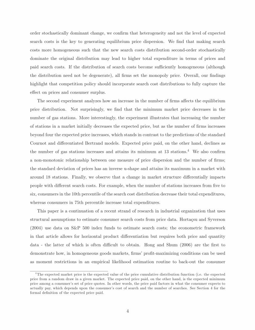
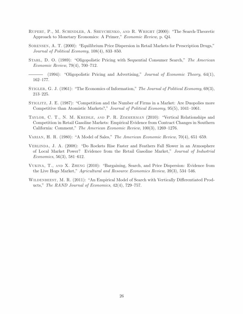
To analyze the relationship between search costs and census tract level characteristics, isolated
markets are further restricted to only include markets where all gas stations are located within a
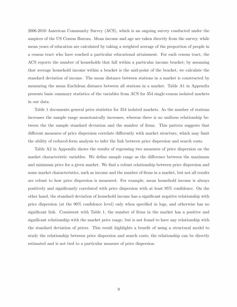
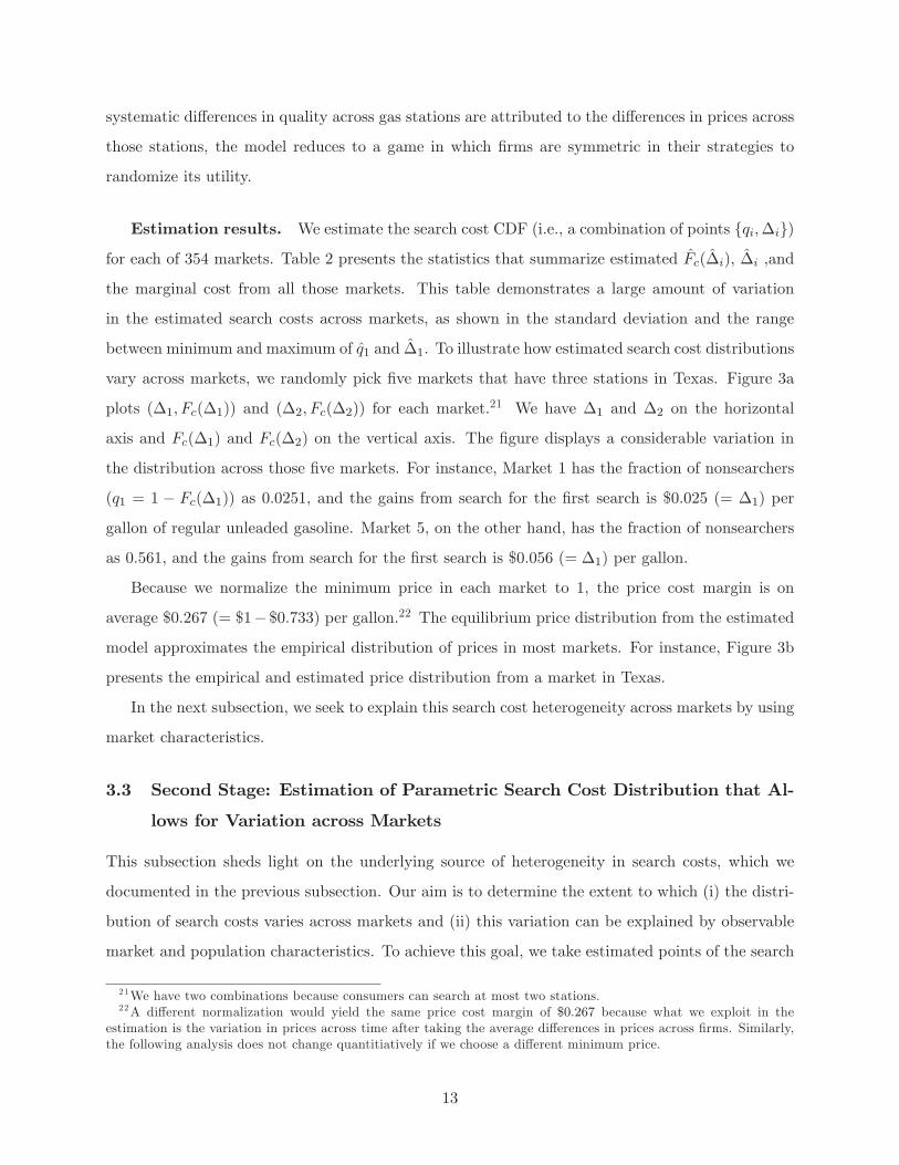
single census tract. Figure 1 depicts a map that contains such an isolated markets with multiple
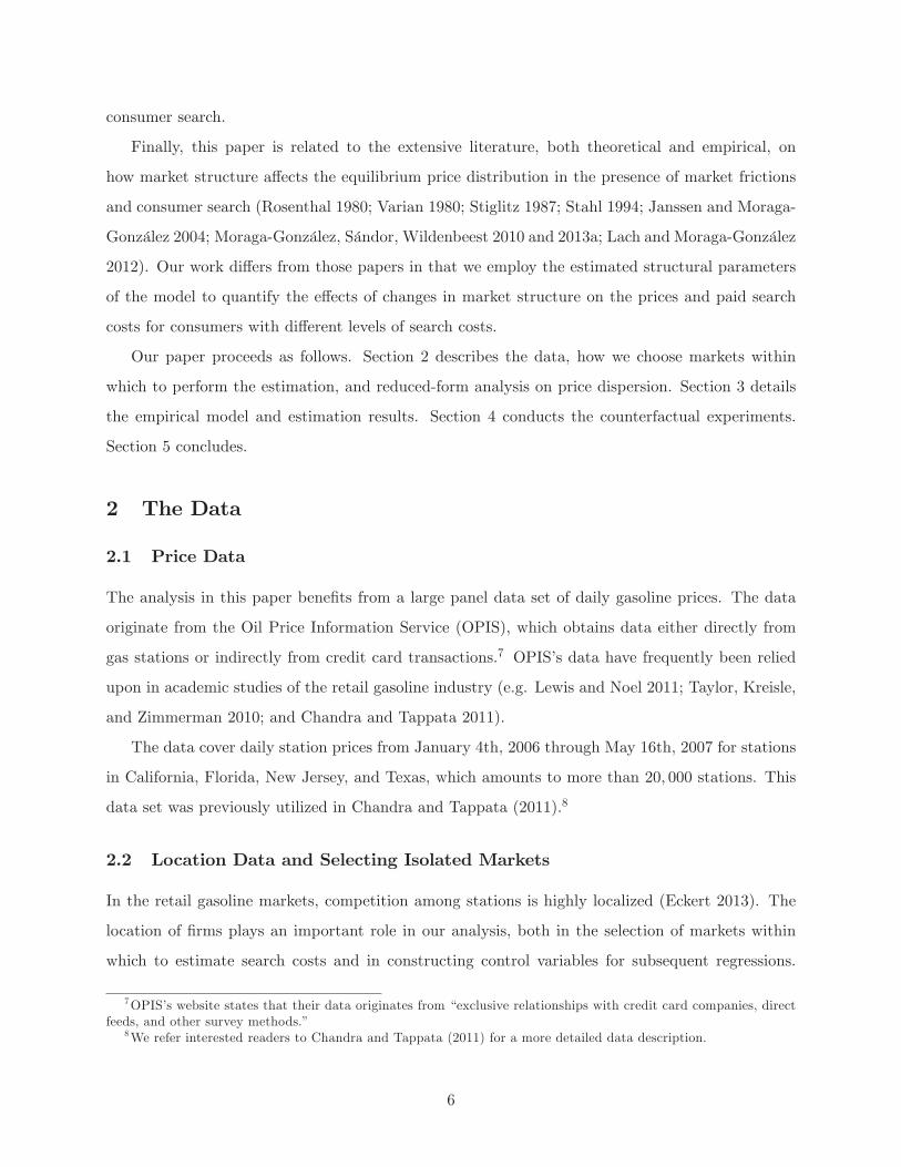
firms and a single census tract (“Market 1”). Using this market definition, we estimate the model
using 11, 736 price observations from 1, 127 stations in 354 isolated (and single census tract) mar-
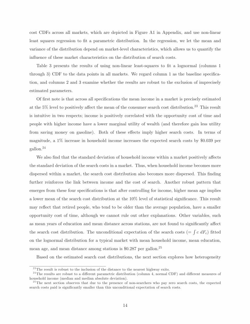
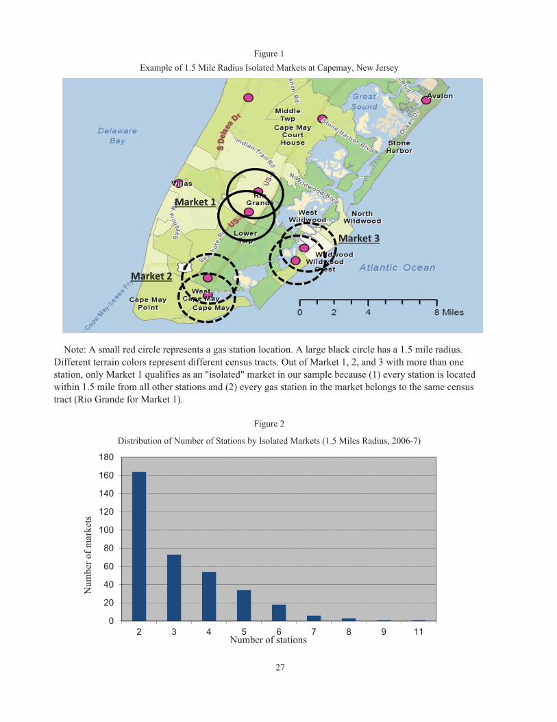
kets. Figure 2 shows the distribution of those markets by market structure. Although our market
definition still contains some potential issues, such as people may purchase gasoline not only where
they live, but also where they commute for work, the requirements for the market definition in this
9For example, see Hastings (2004), Barron, Taylor, and Umbeck (2004), Lewis (2008), and Remer (2013).10For example, suppose three firms, A, B, and C, are located one mile apart in sequence along a road. Using a
cutoff distance of 1.5 miles for the radius, we obtain three markets, A and B, A, B, and C, and B and C. It would,however, be inappropriate to treat market outcomes from these three markets as three independent observations todraw inferences on each of those markets because firm A and C’s pricing is dependent through firm B’s pricing.
7
study are more stringent than those used by most of the existing literature.11
2.3 Cost data
The structural model that we estimate requires only price data, and reconciles the observed price
dispersion as a consequence of vertical product differentiation and heterogeneity in consumers’ cost
of search. In our data, however, prices may vary over time in response to changes in the wholesale
cost of gasoline. To minimize the effect of marginal cost changes on the observed price dispersion,
the model is estimated using the 30 day window in the data where the variation in wholesale price
of gasoline is minimized. As the price at which each retailer purchased their product is privately
negotiated and unavailable, we utilize the price of wholesale gasoline traded on the New York
Mercantile Exchange (NYMEX), which is likely to be highly correlated with actual marginal costs.
These data are commonly employed as a measure of marginal cost in studies of the retail gasoline
industry.12 We estimate the model using price data from March 3rd through April 1st, 2006, where
the standard deviation of the daily price of wholesale unleaded fuel shipped from the NY Harbor
was 6.3 cents per gallon.13
2.4 Descriptive Evidence of Price Dispersion
Both survey evidence and the economic literature demonstrate that consumer search plays an
important role in the retail gasoline industry. The National Association for Convenience and Fuel
Retailing (NACS) has been surveying gasoline consumers since 2007 and has consistently found
that price is overwhelmingly the most important factor in buying gasoline.14 They also find that
about 68% of people would drive five minutes out of their way to save 5 cents per gallon, but only
36% of people would drive ten minutes to save the same amount. Similar results throughout the
survey suggest that (i) a large fraction of people search to save money on gasoline expenditures
and (ii) the intensity with which customers search varies.
We run OLS regressions to document the relationship between measures of price dispersion
and market characteristics. The census-level data used as explanatory variables is taken from the
11A notable exception is Houde (2012), who focuses on the Quebec City gasoline market and takes commutingroutes into account.12See, for example, Borenstein, Cameron, and Gilbert (1997), Velinda (2008), and Lewis (2011).13Note also that there are brief windows in the data set where price data are missing. These days were a priori
excluded as potential times over which to perform the estimation.14See http://www.nacsonline.com/YourBusiness/FuelsReports/GasPrices_2013/Pages/Consumers-React-to-Gas-
Prices.aspx.
8
2006-2010 American Community Survey (ACS), which is an ongoing survey conducted under the
auspices of the US Census Bureau. Mean income and age are taken directly from the survey, while
mean years of education are calculated by taking a weighted average of the proportion of people in
a census tract who have reached a particular educational attainment. For each census tract, the
ACS reports the number of households that fall within a particular income bracket; by assuming
that average household income within a bracket is the mid-point of the bracket, we calculate the
standard deviation of income. The mean distance between stations in a market is constructed by
measuring the mean Euclidean distance between all stations in a market. Table A1 in Appendix
presents basic summary statistics of the variables from ACS for 354 single-census isolated markets
in our data.
Table 1 documents general price statistics for 354 isolated markets. As the number of stations
increases the sample range monotonically increases, whereas there is no uniform relationship be-
tween the the sample standard deviation and the number of firms. This pattern suggests that
different measures of price dispersion correlate differently with market structure, which may limit
the ability of reduced-form analysis to infer the link between price dispersion and search costs.
Table A2 in Appendix shows the results of regressing two measures of price dispersion on the
market characteristic variables. We define sample range as the difference between the maximum
and minimum price for a given market. We find a robust relationship between price dispersion and
some market characteristics, such as income and the number of firms in a market, but not all results
are robust to how price dispersion is measured. For example, mean household income is always
positively and significantly correlated with price dispersion with at least 95% confidence. On the
other hand, the standard deviation of household income has a significant negative relationship with
price dispersion (at the 90% confidence level) only when specified in logs, and otherwise has no
significant link. Consistent with Table 1, the number of firms in the market has a positive and
significant relationship with the market price range, but is not found to have any relationship with
the standard deviation of prices. This result highlights a benefit of using a structural model to
study the relationship between price dispersion and search costs; the relationship can be directly
estimated and is not tied to a particular measure of price dispersion.
9
3 Model Estimation
3.1 Empirical Model of Search and Price Equilibrium
This subsection introduces a non-sequential search model based on Burdett and Judd (1983) and
explains how the model can be used to estimate the distribution of consumer search costs.15 Our
model presentation borrows from Hong and Shum (2006) and Moraga-González and Wildenbeest
(2008).
We first consider a set of gas stations selling a homogeneous product to a continuum of consumers
that are identical except for their search costs that are unobservable to the firm.16 Firms, however,
do know the distribution of consumer search costs. Each firm in the market simultaneously chooses
its price, p; the cumulative equilibrium price distribution is denoted as Fp, where p¯and p are
the lower and upper bound, respectively, of the support of Fp. Firms have constant and identical
marginal costs of production, denoted as r. In equilibrium, firms play mixed strategies and therefore
vary their prices over time.1718
Consumers draw an i.i.d. search cost, c ≥ 0, from the cumulative search cost distribution, Fc.
All consumers have an inelastic demand for a unit of gasoline. Consumers know the distribution
of market prices,Fp(p), but they do not know individual firms’ prices. Consumers receive one free
price quote and must pay a cost, c, for each additional quote. Consumers learn the realization of
prices after deciding how many additional quotes to obtain, including no additional quote, which
implies the consumer goes with the free quote. With a sample of l(≥ 1) gas prices from l stations,
each consumer purchases one unit from the lowest-priced gas station in their sample. A consumer’s
problem is to minimize the total expected expenditure of purchasing a product by choosing the
15We assume that consumers search non-sequentially in retail gasoline markets. See De Los Santos, Hortaçsu, andWildenbeest (2012) and Honka and Chintagunta (2013) for discussions and empirical testing of these two strategies.16Wildenbeest (2011) demonstrates that specifying the model in terms of utility, rather than price, allows for vertical
product differentiation to be incorporated into the model, and controlled for in the estimation by simply adding afixed-effect. While our empirical model accounts for vertical product differentiation, for expositional purposes in thissection, we discuss a homogeneous product market where the price p is the strategic variable. All of the subsequentdiscussions go through if we replace price with utility.17Several empirical works document that the pricing of retail gasoline stations is consistent with a mixed strategy;
see Lewis (2008), Hosken, McMillan and Taylor (2008), Lach and Moraga-González (2009), and Chandra and Tappata(2011).18For expositional simplicity, we present the model by assuming products are homogeneous. Our empirical model
extends this framework by assuming that firms play mixed strategies in utilities, which consist of price and qualityof a product (Wildenbeest 2011). See the next subsection for details.
10
number of gas stations to search, l − 1, where
l = argminl≥1
c · (l − 1) +∫ p
p¯
l · p(1− Fp(p))l−1f(p)dp.
The first term, c(l − 1), is the total costs of search.19 The second term is the expected price paid
for the product when a consumer has l quotes from l stations. (1−Fp(p))l−1 is the probability thatall other stations charge a price higher than p. By searching i+ 1 rather than i stores, a consumer
obtains an expected marginal savings, which is denoted as Δi ≡ Ep1:i − Ep1:i+1, i = 1, 2, ... Here,p1:i represents the minimum price when a consumer takes i draws from Fp. Accordingly, a consumer
with search cost c will sample i stores when Δi−1 > c > Δi. A consumer with c = Δi is indifferent
between searching i stores and i+1 stores. The proportion of consumers with i price quotes qi will
be q1 ≡ 1− Fc(Δ1) and qi ≡ Fc(Δi−1)− Fc(Δi) for i ≥ 2.Firms maximize profits by choosing a symmetric, mixed-pricing strategy Fp for all p ∈ [p
¯, p].
Based on the consumer behavior, each firm’s total profit can be denoted as Π(p) = (p− r)[∑Ni=1 qi ·
iN (1 − Fp(p))i−1]. The firms’ profit-maximizing mixed strategies imply a condition that each firmis indifferent between charging the monopoly price p and any other price p ∈ [p
¯, p], namely
(p− r)q1N
= (p− r)[N∑i=1
qi · iN(1− Fp(p))i−1], (1)
where r is the common marginal cost of selling gasoline for each gas station. In words, firms face a
trade-off between setting a high price and selling to less informed customers or setting a low price
and capturing more informed customers. In equilibrium, firms are indifferent between all points
in the price distribution and therefore maximize profits by playing a mixed strategy over the price
distribution. Solving equation (1) for price allows us to represent price as the inverse function
p(z) =q1(p− r)∑N
i=1 iqi(1− z)i−1+ r, (2)
where z = Fp(p).
19We subtract 1 because the first quote is free.
11
3.2 First Stage: Nonparametric Estimation of Search Cost at the Market Level
Our first stage estimation strategy is based on Hong and Shum (2006) and the extensions developed
in Moraga-González and Wildenbeest (2008) and Wildenbeest (2011). The Hong and Shum (2006)
framework allows the distribution of consumer search costs to be recovered using price data alone
by rationalizing the observed price dispersion as a consequence of search costs. We apply this
methodology to each geographically isolated retail gasoline market to document the heterogeneity
of search costs across markets.
To identify the model parameters, we use the equilibrium condition specified in equation (1),
that in a mixed strategy equilibrium, expected profits are the same for all prices in the support
of the equilibrium price distribution. We conduct nonparametric estimation using this optimality
condition.
We conduct the maximum likelihood technique developed by Moraga-González and Wildenbeest
(2008). Denoting the number of gas stations in a market by N and the number of price observations
in that market by M , we employ the MLE estimation strategy to obtain the estimated model
parameter θMLE = {qi}N−1i=1 such that:
θMLE = arg max{qi}N−1i=1
M−1∑l=2
log fp(pl; q1, .., qN ),
where fp is the density for Fp and Fp(pl) solves equation (1).20 The maximum likelihood routine
yields estimates of a non-parametric search cost CDF represented by a combination of points
{qi,Δi}.Finally, we control for potential vertical differentiation by gas stations within a market using
Wildenbeest (2011). This method extends Hong and Shum (2006) such that firms play mixed
strategies in consumer utility, where uj = δj − pj and δj is the value consumers realize frompurchasing one unit of the good from station j. To implement this model, we parameterize the
price at firm j at time t, pjt, as
pjt = α+ δj + εjt, (3)
and perform the fixed effects regression specified by equation (3) for a given market to recover
δj .We then construct the utility from station j by setting ujt = pjt − δj . By assuming that any
20Appendix provides the representation of fp in Fp, qi, p, and r.
12
systematic differences in quality across gas stations are attributed to the differences in prices across
those stations, the model reduces to a game in which firms are symmetric in their strategies to
randomize its utility.
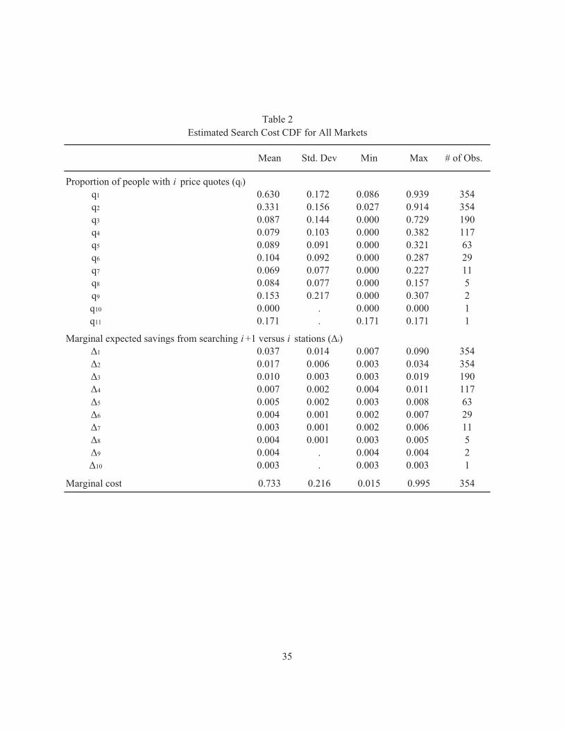
Estimation results. We estimate the search cost CDF (i.e., a combination of points {qi,Δi})for each of 354 markets. Table 2 presents the statistics that summarize estimated Fc(Δi), Δi ,and
the marginal cost from all those markets. This table demonstrates a large amount of variation
in the estimated search costs across markets, as shown in the standard deviation and the range
between minimum and maximum of q1 and Δ1. To illustrate how estimated search cost distributions
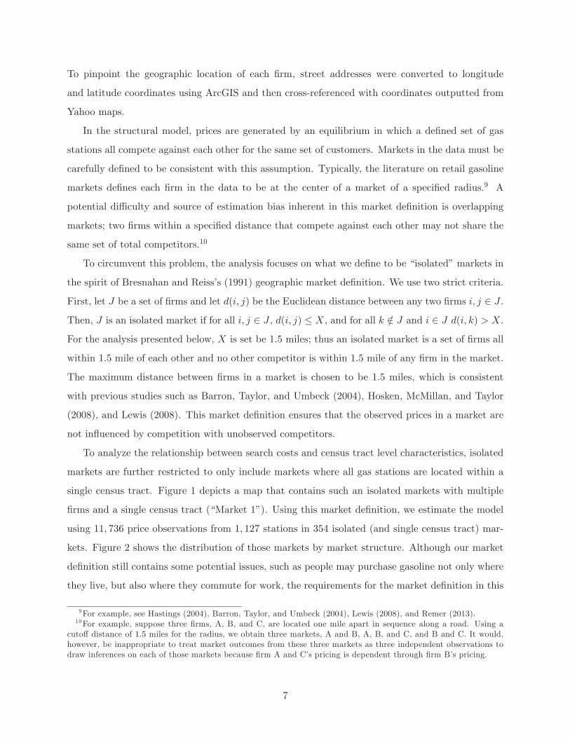
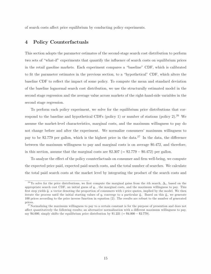
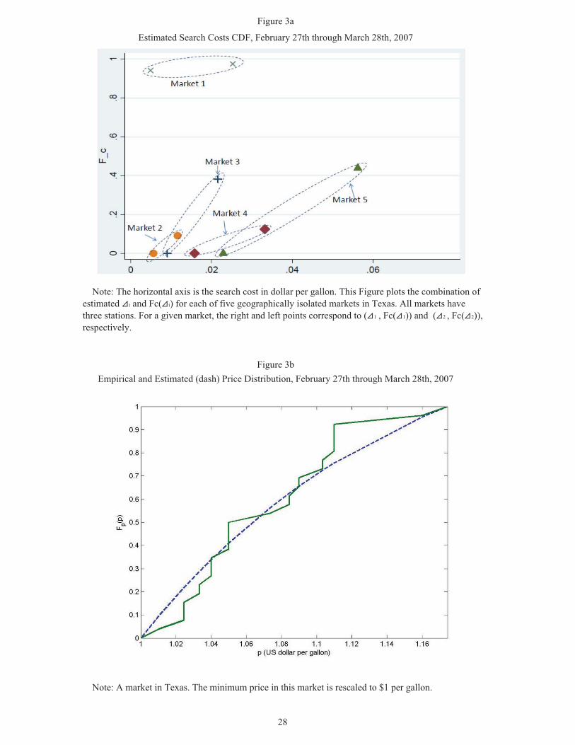
vary across markets, we randomly pick five markets that have three stations in Texas. Figure 3a
plots (Δ1, Fc(Δ1)) and (Δ2, Fc(Δ2)) for each market.21 We have Δ1 and Δ2 on the horizontal
axis and Fc(Δ1) and Fc(Δ2) on the vertical axis. The figure displays a considerable variation in
the distribution across those five markets. For instance, Market 1 has the fraction of nonsearchers
(q1 = 1 − Fc(Δ1)) as 0.0251, and the gains from search for the first search is $0.025 (= Δ1) per
gallon of regular unleaded gasoline. Market 5, on the other hand, has the fraction of nonsearchers
as 0.561, and the gains from search for the first search is $0.056 (= Δ1) per gallon.
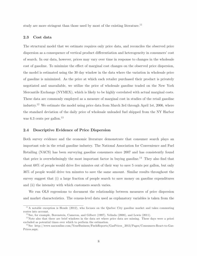
Because we normalize the minimum price in each market to 1, the price cost margin is on
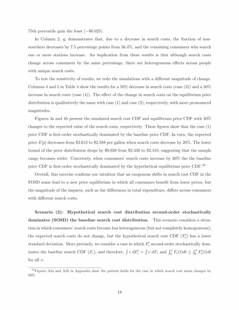
average $0.267 (= $1− $0.733) per gallon.22 The equilibrium price distribution from the estimated
model approximates the empirical distribution of prices in most markets. For instance, Figure 3b
presents the empirical and estimated price distribution from a market in Texas.
In the next subsection, we seek to explain this search cost heterogeneity across markets by using
market characteristics.
3.3 Second Stage: Estimation of Parametric Search Cost Distribution that Al-
lows for Variation across Markets
This subsection sheds light on the underlying source of heterogeneity in search costs, which we
documented in the previous subsection. Our aim is to determine the extent to which (i) the distri-
bution of search costs varies across markets and (ii) this variation can be explained by observable
market and population characteristics. To achieve this goal, we take estimated points of the search
21We have two combinations because consumers can search at most two stations.22A different normalization would yield the same price cost margin of $0.267 because what we exploit in the
estimation is the variation in prices across time after taking the average differences in prices across firms. Similarly,the following analysis does not change quantitiatively if we choose a different minimum price.
13
cost CDFs across all markets, which are depicted in Figure A1 in Appendix, and use non-linear
least squares regression to fit a parametric distribution. In the regression, we let the mean and
variance of the distribution depend on market-level characteristics, which allows us to quantify the
influence of these market characteristics on the distribution of search costs.
Table 3 presents the results of using non-linear least-squares to fit a lognormal (columns 1
through 3) CDF to the data points in all markets. We regard column 1 as the baseline specifica-
tion, and columns 2 and 3 examine whether the results are robust to the exclusion of imprecisely
estimated parameters.
Of first note is that across all specifications the mean income in a market is precisely estimated
at the 5% level to positively affect the mean of the consumer search cost distribution.23 This result
is intuitive in two respects; income is positively correlated with the opportunity cost of time and
people with higher income have a lower marginal utility of wealth (and therefore gain less utility
from saving money on gasoline). Both of these effects imply higher search costs. In terms of
magnitude, a 1% increase in household income increases the expected search costs by $0.039 per
gallon.24
We also find that the standard deviation of household income within a market positively affects
the standard deviation of the search costs in a market. Thus, when household income becomes more
dispersed within a market, the search cost distribution also becomes more dispersed. This finding
further reinforces the link between income and the cost of search. Another robust pattern that
emerges from these four specifications is that after controlling for income, higher mean age implies
a lower mean of the search cost distribution at the 10% level of statistical significance. This result
may reflect that retired people, who tend to be older than the average population, have a smaller
opportunity cost of time, although we cannot rule out other explanations. Other variables, such
as mean years of education and mean distance across stations, are not found to significantly affect
the search cost distribution. The unconditional expectation of the search costs (=∫c dFc) fitted
on the lognormal distribution for a typical market with mean household income, mean education,
mean age, and mean distance among stations is $0.287 per gallon.25
Based on the estimated search cost distributions, the next section explores how heterogeneity
23The result is robust to the inclusion of the distance to the nearest highway exits.24The results are robust to a different parametric distribution (column 4, normal CDF) and different measures of
household income (median and median absolute deviation).25The next section observes that due to the presence of non-searchers who pay zero search costs, the expected
search costs paid is significantly smaller than this unconditional expectation of search costs.
14
of search costs affect price equilibrium by conducting policy experiments.
4 Policy Counterfactuals
This section adopts the parameter estimates of the second-stage search cost distribution to perform
two sets of “what-if” experiments that quantify the influence of search costs on equilibrium prices
in the retail gasoline markets. Each experiment compares a “baseline” CDF, which is calibrated
to fit the parameter estimates in the previous section, to a “hypothetical” CDF, which alters the
baseline CDF to reflect the impact of some policy. To compute the mean and standard deviation
of the baseline lognormal search cost distribution, we use the structurally estimated model in the
second stage regression and the average value across markets of the right-hand-side variables in the
second stage regression.
To perform each policy experiment, we solve for the equilibrium price distributions that cor-
respond to the baseline and hypothetical CDFs (policy 1) or number of stations (policy 2).26 We
assume the market-level characteristics, marginal costs, and the maximum willingness to pay do
not change before and after the experiment. We normalize consumers’ maximum willingness to
pay to be $2.779 per gallon, which is the highest price in the data.27 In the data, the difference
between the maximum willingness to pay and marginal costs is on average $0.472, and therefore,
in this section, assume that the marginal costs are $2.307 (= $2.779− $0.472) per gallon.To analyze the effect of the policy counterfactuals on consumer and firm well-being, we compute
the expected price paid, expected paid search costs, and the total number of searches. We calculate
the total paid search costs at the market level by integrating the product of the search costs and
26To solve for the price distributions, we first compute the marginal gains from the ith search, Δi, based on theappropriate search cost CDF, an initial guess of qi , the marginal costs, and the maximum willingness to pay. Thisfirst step yields qi a vector denoting the proportion of consumers with i price quotes, implied by the model. We theniterate the process until the initial starting values of qi converge to a particular qi. Based on this qi, we generate100 prices according to the price inverse function in equation (2). The results are robust to the number of generatedprices.27Normalizing the maximum willingness to pay to a certain constant is for the purpose of presention and does not
affect quantitatively the following results; an alternative normalization with a different maximum willingness to pay,say $4.000, simply shifts the equilibrium price distribution by $1.221 (= $4.000− $2.779).
15

the number of searches over the search cost CDF. Specifically,
E[cpaid] =N∑i=1{(i− 1)
QN+2−i∫
QN+1−i
cdFc}
where Qi = 1−N+1−i∑s=1
qs if N + 1− i ≥ 1 and Qi = 1 otherwise ,
and N is the number of stations in that market. For instance, the expected search cost paid in a
market with three station is
E[cpaid] = 2
q3∫0
cdFc +
q2+q3∫q3
cdFc,
and the first and the second term is the expected paid search costs for people who search twice and
once, respectively. Similarly, the expected price paid is obtained by first calculating the expected
price conditional on the number of times a consumer searches, and then integrating over the number
of searches: E[ppaid] = Epq1 +N∑i=2{Ep − (
i−1∑s=1Δs)}qi. For instance, the expected price paid in a
market with three stations is
E[ppaid] = Ep︸︷︷︸Expected price for non searchers
∗q1 + (Ep−Δ1)︸ ︷︷ ︸Expected price for people who search once
∗q2
+ (Ep−Δ1 −Δ2)︸ ︷︷ ︸Expected price for people who search twice
∗q3.
To demonstrate how certain policies differentially affect consumers with different search costs,
we present results for consumers in the 10th, 25th, 50th, and 75th percentiles of the search cost
distribution.
4.1 Policy Experiment 1: A Change in the Costs of Search
We first examine an exogenous change in the cost of search, such as a technological advance in
searching for gas prices or a government policy that publicizes gas prices on a website. Such a
change would involve two aspects: change in the mean and change in the standard deviation of
a distribution, and we discuss each aspect separately. In particular, we consider two scenarios in
which the baseline search cost CDF (i) first-order stochastically dominates the hypothetical search
cost CDF or (ii) is second-order stochastically dominated by the hypothetical search cost CDF.
16

Scenario (1): All consumers’ cost of search decreases, and the baseline search cost
CDF first-order stochastically dominates the hypothetical search cost distribution.
This scenario considers a situation in which expected value of search costs decrease (or increase)
for every consumer, while keeping the variability (i.e., standard deviation of the distribution) the
same. A decrease in search costs would represent a situation in which consumers’ search effort
has been reduced due to technological developments, such as smartphones and related apps, that
affect the ease of finding gasoline price quotes. As a consequence, the hypothetical search cost
CDF (F ′c) is first-order stochastically dominated by the baseline search CDF, (Fc): F ′c(t) > Fc(t)
for any t > 0.28 Given the significant relationship estimated in the previous section between search
costs and household income, the counterfactual experiments can also be interpreted as a change in
household income, rather than as a policy that directly alters the cost of search.
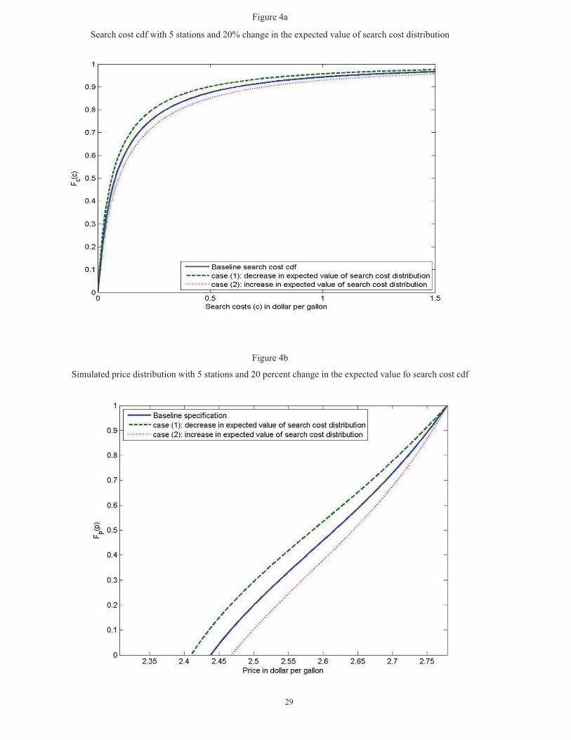
Table 4 presents the simulation results for a market with five firms for the baseline specification,
a 20% decrease in search costs (case (1)), and a 20% increase in search costs (case (2)). To interpret
the experiment as a change in household income, cases (1) and (2) and the baseline correspond
to observationally equivalent markets except for the average household income, which is $9, 288,
$243, 917 and $62, 270, respectively.29 Below we mainly discuss the difference between the baseline
and the 20% decrease in search costs in case (1) in the second column in Table 4. The expected price
paid, on average, decreases by $0.035 from $2.573 (baseline). The decrease in the actual price paid
differs across consumers with different search costs. For instance, consumers in the 50th percentile
experience the largest decrease in the price paid (−$0.090 = $2.523− $2.613), whereas consumersin the 75th percentile experience the smallest decrease (−$0.025 = $2.588−$2.613) among the fourcategories of consumers (10%, 25%, 50%, and 75%tile).
We observe the policy change affects consumers with different search costs differently for other
measures as well. The expected paid search costs decrease on average by $0.003 from $0.017.
The decrease is the largest for consumers in the 25th percentile (−$0.010), but people in the 50thpercentile actually increase the paid search costs by $0.062 due to an increased number of search.
With respect to total consumer expenditure, which is the sum of expected price paid and paid
search costs, consumers in the 25th percentile gain the most (−$0.042) whereas consumers in the
28By contrast, an increase in search costs would represent a situation in which search behavior becomes morecumbersome due to an intentional price obfuscation by retailers (Ellison and Ellison 2009) or an installation of agovernment policy, such as one that prohibits the operation of price comparison gasoline websites (e.g., gasbuddy.com).In this scenario, the hypothetical search cost CDF (F ′c) first-order stochastically dominates the baseline CDF (Fc).29This sample range in household income roughly corresponds to the observed mean household income’s minimum
and maximum (Table A1 in Appendix).
17
75th percentile gain the least (−$0.025).In Column 2, qi demonstrates that, due to a decrease in search costs, the fraction of non-
searchers decreases by 7.5 percentage points from 56.4%, and the remaining consumers who search
one or more stations increase. An implication from these results is that although search costs
change across consumers by the same percentage, there are heterogeneous effects across people
with unique search costs.
To test the sensitivity of results, we redo the simulations with a different magnitude of change.
Columns 4 and 5 in Table 4 show the results for a 50% decrease in search costs (case (3)) and a 50%
increase in search costs (case (4)). The effect of the change in search costs on the equilibrium price
distribution is qualitatively the same with case (1) and case (2), respectively, with more pronounced
magnitudes.
Figures 4a and 4b present the simulated search cost CDF and equilibrium price CDF with 20%
changes to the expected value of the search costs, respectively. These figures show that the case (1)
price CDF is first-order stochastically dominated by the baseline price CDF. In turn, the expected
price E[p] decreases from $2.613 to $2.588 per gallon when search costs decrease by 20%. The lower
bound of the price distribution drops by $0.028 from $2.438 to $2.410, suggesting that the sample
range becomes wider. Conversely, when consumers’ search costs increase by 20% the the baseline
price CDF is first-order stochastically dominated by the hypothetical equilibrium price CDF.30
Overall, this exercise confirms our intuition that an exogenous shifts in search cost CDF in the
FOSD sense lead to a new price equilibrium in which all consumers benefit from lower prices, but
the magnitude of the impacts, such as the differences in total expenditure, differs across consumers
with different search costs.
Scenario (2): Hypothetical search cost distribution second-order stochastically
dominates (SOSD) the baseline search cost distribution. This scenario considers a situa-
tion in which consumers’ search costs become less heterogeneous (but not completely homogeneous);
the expected search costs do not change, but the hypothetical search cost CDF (F ′c) has a lower
standard deviation. More precisely, we consider a case in which F ′c second-order stochastically dom-
inates the baseline search CDF (Fc), and therefore,∫c dF ′c =
∫c dFc and
∫ x0 Fc(t)dt ≥
∫ x0 F
′c(t)dt
for all x.
30Figures A2a and A2b in Appendix show the pattern holds for the case in which search cost mean changes by50%.
18
To perform this experiment, the standard deviation parameter of the lognormal CDF, σ, for the
hypothetical distribution, F ′c, is set to be 15% lower than the standard deviation for the baseline
lognormal distribution, Fc. We then calculate the mean parameter, μ, for the hypothetical distri-
bution that yields the same unconditional expected search costs,∫c dFc =
∫c dF ′c = $0.287 per
gallon of gasoline.31 Using Fc and F ′c we simulate gas stations’ optimal pricing decisions under the
baseline and hypothetical scenarios.32
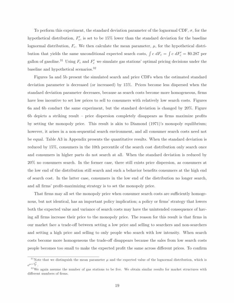
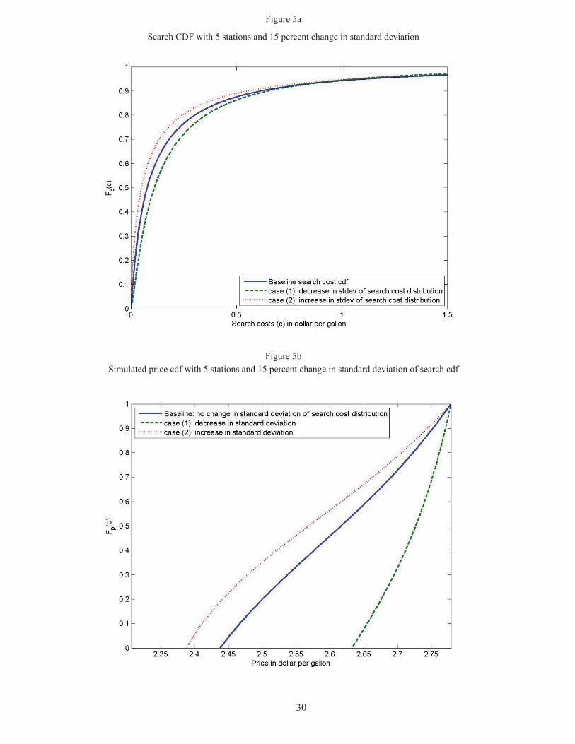
Figures 5a and 5b present the simulated search and price CDFs when the estimated standard
deviation parameter is decreased (or increased) by 15%. Prices become less dispersed when the
standard deviation parameter decreases, because as search costs become more homogeneous, firms
have less incentive to set low prices to sell to consumers with relatively low search costs. Figures
6a and 6b conduct the same experiment, but the standard deviation is changed by 20%. Figure
6b depicts a striking result — price dispersion completely disappears as firms maximize profits
by setting the monopoly price. This result is akin to Diamond (1971)’s monopoly equilibrium;
however, it arises in a non-sequential search environment, and all consumer search costs need not
be equal. Table A3 in Appendix presents the quantitative results. When the standard deviation is
reduced by 15%, consumers in the 10th percentile of the search cost distribution only search once
and consumers in higher parts do not search at all. When the standard deviation is reduced by
20% no consumers search. In the former case, there still exists price dispersion, as consumers at
the low end of the distribution still search and such a behavior benefits consumers at the high end
of search cost. In the latter case, consumers in the low end of the distribution no longer search,
and all firms’ profit-maximizing strategy is to set the monopoly price.
That firms may all set the monopoly price when consumer search costs are sufficiently homoge-
nous, but not identical, has an important policy implication; a policy or firms’ strategy that lowers
both the expected value and variance of search costs may have the unintended consequence of hav-
ing all firms increase their price to the monopoly price. The reason for this result is that firms in
our market face a trade-off between setting a low price and selling to searchers and non-searchers
and setting a high price and selling to only people who search with low intensity. When search
costs become more homogeneous the trade-off disappears because the sales from low search costs
people becomes too small to make the expected profit the same across different prices. To confirm
31Note that we distinguish the mean parameter μ and the expected value of the lognormal distribution, which is
eμ+σ2
2 .32We again assume the number of gas stations to be five. We obtain similar results for market structures with
different numbers of firms.
19

this point, we run a variant of the last policy experiment; in addition to reducing the standard de-
viation of search costs, we also decrease the expected value of the search cost distribution. Figures
A3a and A3b in Appendix presents the results of decreasing the expected value of the search cost
distribution by 10% and reducing the standard deviation by 20% and 22%, respectively. When
the standard deviation is reduced by 20%, we have a price dispersion unlike the previous case in
Figure 6b because it is cheaper to search due to a reduced search costs by 10%. When the standard
deviation is reduced by 22%, however, no consumers search even when the expected value of the
search costs decreases by 10%.
4.2 Policy Experiment 2: A Change in Market Structure
Now we investigate how, holding the search cost distribution constant, different market structure
affects the equilibrium price distribution and search behavior differently. This experiment informs
how firms and consumers respond to an increase in competition via entry of firms into the retail
gasoline market.
To conduct this experiment, we assume that exogenous changes in market structure do not
affect the distribution of consumer search costs, and use the same mean and standard deviation
for the lognormal search costs distribution we estimated in the previous section and used in the
experiment above.
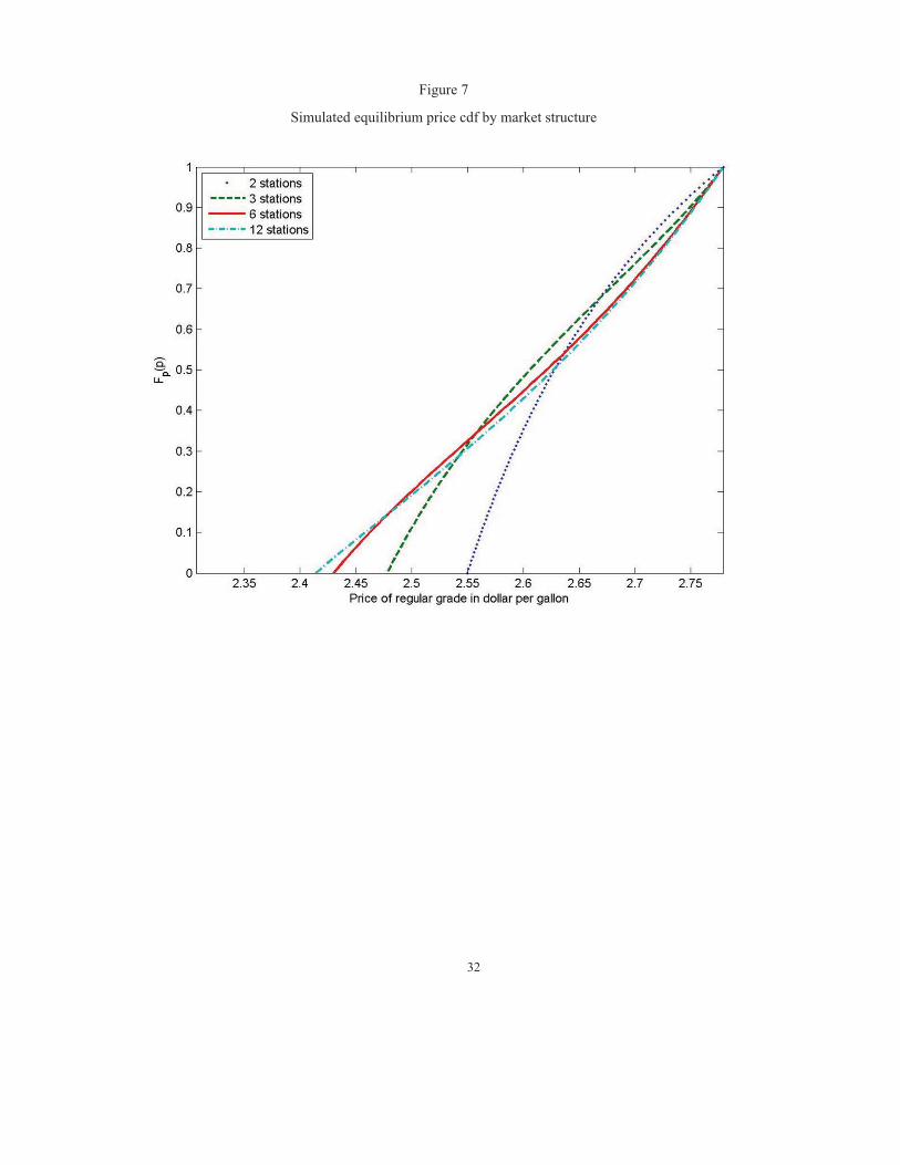
Figure 7 presents the simulated price distribution for hypothetical markets with two, three, six,
and twelve gas stations. Two patterns emerge from this figure. First, the minimum price decreases
as the number of stations increase, and, as the maximum price remains fixed at $2.779, the price
range (= pmax − pmin) increases in the number of stations. Second, beyond three stations, thedifference in the price distributions across markets becomes considerably smaller. Although the
minimum price declines when a market becomes more competitive, those who do not search are
worse off in less concentrated markets with more than three firms. Indeed, Figure 7 shows that, for
prices below $2.48, the simulated price CDF for a market with 12 stations is flatter than the CDF
with six stations. This pattern implies that the lower minimum price in a market with 12 stations
will be compensated by a steeper CDF above $2.48, which means that consumers with high search
costs may face higher prices when the number of firms increase from six to twelve.
Figure 8a further analyzes these points in detail by displaying the summary statistics by market
structure. The figure demonstrates how equilibrium price dispersion and paid search costs change
with the number of firms. Again, the minimum price declines monotonically with the number of
20
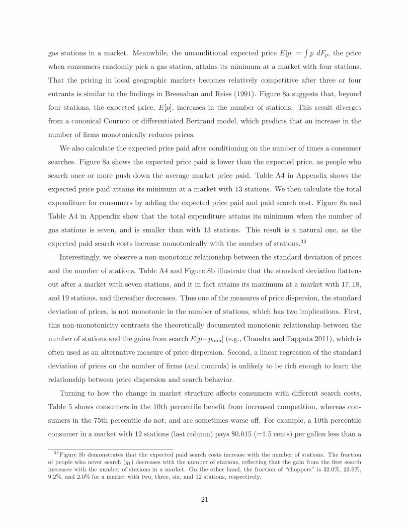
gas stations in a market. Meanwhile, the unconditional expected price E[p] =∫p dFp, the price
when consumers randomly pick a gas station, attains its minimum at a market with four stations.
That the pricing in local geographic markets becomes relatively competitive after three or four
entrants is similar to the findings in Bresnahan and Reiss (1991). Figure 8a suggests that, beyond
four stations, the expected price, E[p], increases in the number of stations. This result diverges
from a canonical Cournot or differentiated Bertrand model, which predicts that an increase in the
number of firms monotonically reduces prices.
We also calculate the expected price paid after conditioning on the number of times a consumer
searches. Figure 8a shows the expected price paid is lower than the expected price, as people who
search once or more push down the average market price paid. Table A4 in Appendix shows the
expected price paid attains its minimum at a market with 13 stations. We then calculate the total
expenditure for consumers by adding the expected price paid and paid search cost. Figure 8a and
Table A4 in Appendix show that the total expenditure attains its minimum when the number of
gas stations is seven, and is smaller than with 13 stations. This result is a natural one, as the
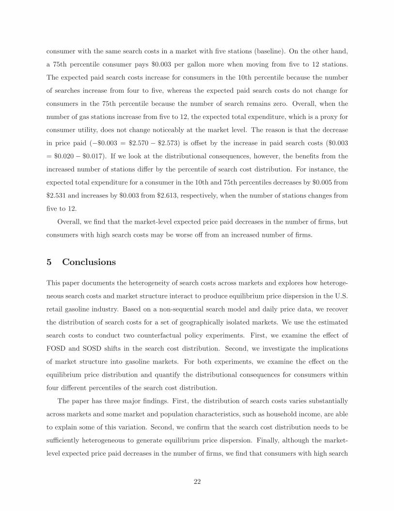
expected paid search costs increase monotonically with the number of stations.33
Interestingly, we observe a non-monotonic relationship between the standard deviation of prices
and the number of stations. Table A4 and Figure 8b illustrate that the standard deviation flattens
out after a market with seven stations, and it in fact attains its maximum at a market with 17, 18,
and 19 stations, and thereafter decreases. Thus one of the measures of price dispersion, the standard
deviation of prices, is not monotonic in the number of stations, which has two implications. First,
this non-monotonicity contrasts the theoretically documented monotonic relationship between the
number of stations and the gains from search E[p−pmin] (e.g., Chandra and Tappata 2011), which isoften used as an alternative measure of price dispersion. Second, a linear regression of the standard
deviation of prices on the number of firms (and controls) is unlikely to be rich enough to learn the
relationship between price dispersion and search behavior.
Turning to how the change in market structure affects consumers with different search costs,
Table 5 shows consumers in the 10th percentile benefit from increased competition, whereas con-
sumers in the 75th percentile do not, and are sometimes worse off. For example, a 10th percentile
consumer in a market with 12 stations (last column) pays $0.015 (=1.5 cents) per gallon less than a
33Figure 8b demonstrates that the expected paid search costs increase with the number of stations. The fractionof people who never search (q1) decreases with the number of stations, reflecting that the gain from the first searchincreases with the number of stations in a market. On the other hand, the fraction of “shoppers” is 32.0%, 23.9%,9.2%, and 2.0% for a market with two, three, six, and 12 stations, respectively.
21
consumer with the same search costs in a market with five stations (baseline). On the other hand,
a 75th percentile consumer pays $0.003 per gallon more when moving from five to 12 stations.
The expected paid search costs increase for consumers in the 10th percentile because the number
of searches increase from four to five, whereas the expected paid search costs do not change for
consumers in the 75th percentile because the number of search remains zero. Overall, when the
number of gas stations increase from five to 12, the expected total expenditure, which is a proxy for
consumer utility, does not change noticeably at the market level. The reason is that the decrease
in price paid (−$0.003 = $2.570 − $2.573) is offset by the increase in paid search costs ($0.003= $0.020 − $0.017). If we look at the distributional consequences, however, the benefits from the
increased number of stations differ by the percentile of search cost distribution. For instance, the
expected total expenditure for a consumer in the 10th and 75th percentiles decreases by $0.005 from
$2.531 and increases by $0.003 from $2.613, respectively, when the number of stations changes from
five to 12.
Overall, we find that the market-level expected price paid decreases in the number of firms, but
consumers with high search costs may be worse off from an increased number of firms.
5 Conclusions
This paper documents the heterogeneity of search costs across markets and explores how heteroge-
neous search costs and market structure interact to produce equilibrium price dispersion in the U.S.
retail gasoline industry. Based on a non-sequential search model and daily price data, we recover
the distribution of search costs for a set of geographically isolated markets. We use the estimated
search costs to conduct two counterfactual policy experiments. First, we examine the effect of
FOSD and SOSD shifts in the search cost distribution. Second, we investigate the implications
of market structure into gasoline markets. For both experiments, we examine the effect on the
equilibrium price distribution and quantify the distributional consequences for consumers within
four different percentiles of the search cost distribution.
The paper has three major findings. First, the distribution of search costs varies substantially
across markets and some market and population characteristics, such as household income, are able
to explain some of this variation. Second, we confirm that the search cost distribution needs to be
sufficiently heterogeneous to generate equilibrium price dispersion. Finally, although the market-
level expected price paid decreases in the number of firms, we find that consumers with high search
22
costs may be worse off with an increased number of gas stations.
This study includes some simplifying assumptions, and relaxing these provide a future research
agenda. First, studying the effect of entry on pricing assumes the change in market structure is
exogenous. In the long run, however, market structure is determined through endogenous entry
and exit, which is driven by the profitability of a market. Our work serves as a first step toward
understanding the short-run effect of market structure on pricing. Second, the model assumes
that the quantity of gasoline purchased is inelastic to the change in prices. While in the short-run
this may be true, in the long run people may consume less gasoline or substitute from driving
to other transportation methods when the retail gasoline price increases. Third, we assumed a
lognormal search cost distribution. Although this assumption allows us to explore hypothetical
policy counterfactuals, the quantitative results in the simulation are subject to this approximation.
Finally, we abstract from multi-station pricing under joint ownership due to data limitation. This
assumption, however, is inadequate to consider the effect of mergers for the retail gasoline markets.
Allowing for multi-station ownership is an important topic of future research.
Appendix: equilibrium price density
Following Moraga-González and Wildenbeest (2008), applying the implicit function theorem to
equation (1) yields the density for equilibrium price as
fp(p) =
N∑i=1iqi(1− Fp(p))i−1
(p− r)N∑i=1i(i− 1)qi(1− Fp(p))i−2
,
and Fp(pl) solves (pl − r)[N∑i=1
iqiN (1− Fp(pl))i−1] = q1(p−r)
N for all l = 2, ..,M − 1.
References
A��������, M. (2008): “Interactions between Competition and Consumer Policy,” CompetitionPolicy International, 4(1), 97—147.
B����, J. M., B. A. T���, �� J. R. U� ��� (2004): “Number of Sellers, Average Prices,and Price Dispersion,” International Journal of Industrial Organization, 22(8), 1041—1066.
B�, M. R., J. M����, �� P. S������� (2004): “Price Dispersion in the Small and in the
23

Large: Evidence from an Internet Price Comparison Site,” The Journal of Industrial Economics,52(4), 463—496.
(2006): “Information, Search, and Price Dispersion,” in Handbook on Economics andInformation Systems, ed. by T. Hendershott, vol. 1, chap. 6. Elsevier, Amsterdam.
B���������, S., A. C. C�����, �� R. G�� ��� (1997): “Do Gasoline Prices Respond Asym-metrically to Crude Oil Price Changes?,” Quarterly Journal of Economics, 112(1), 305—339.
B������, T. F., �� P. C. R���� (1991): “Entry and Competition in Concentrated Markets,”Journal of Political Economy, 99(5), 977—1009.
B����, J. R., �� A. G���� �� (2002): “Does the Internet Make Markets More Competitive?Evidence from the Life Insurance Industry,” Journal of Political Economy, 110(3), 481—507.
B������, K., �� K. L. J��� (1983): “Equilibrium Price Dispersion,” Econometrica, 51(4),955—969.
C����, A., �� M. T��� (2011): “Consumer search and dynamic price dispersion: anapplication to gasoline markets,” The RAND Journal of Economics, 42(4), 681—704.
D� ��� S����, B., A. H������, �� M. W����� ���� (2012): “Testing Models of ConsumerSearch using Data on Web Browsing and Purchasing Behavior,” American Economic Review,102(6), 2955—2980.
D�����, P. A. (1971): “A Model of Price Adjustment,” Journal of Economic Theory, 3(2),156—168.
E�����, A. (2013): “Empirical Studies of Gasoline Retailing: A Guide to the Literature,” Journalof Economic Surveys, 27(1), 140—166.
E�������, Z., �� G. J. V� ��� B��� (2007): “Empirical Labor Search: A Survey,” Journalof Econometrics, 136(2), 531—564.
E������, G., �� S. F. E������ (2009): “Search, Obfuscation, and Price Elasticities on theInternet,” Econometrica, 77(2), 427—452.
H������, J. S. (2004): “Vertical Relationships and Competition in Retail Gasoline Markets:Empirical Evidence from Contract Changes in Southern California,” American Economic Review,94(1), 317—328.
H���, H., �� M. S��� (2006): “Using Price Distributions to Estimate Search Costs,” TheRAND Journal of Economics, 37(2), 257—275.
H���, E., �� P. C�������� (2013): “Simultaneous or Sequential? Search Strategies in theUS Auto Insurance Industry,” Discussion paper, University of Texas, Dallas.
H������, A., �� C. S������ (2004): “Product Differentiation, Search Costs, and Compe-tition in the Mutual Fund Industry: A Case Study of S&P 500 Index Funds,” The QuarterlyJournal of Economics, 119(2), 403—456.
H�����, D. S., R. S. M�M����, �� C. T. T��� (2008): “Retail Gasoline Pricing: WhatDo We Know?,” International Journal of Industrial Organization, 26(6), 1425—1436.
24

H����, J.-F. (2012): “Spatial Differentiation and Vertical Mergers in Retail Markets for Gasoline,”The American Economic Review, 102(5), 2147—2182.
J�����, M. C., �� J. L. M���-G������� (2004): “Strategic Pricing, Consumer Searchand the Number of Firms,” Review of Economic Studies, 71(4), 1089—1118.
L��, S. (2002): “Existence and Persistence of Price Dispersion: An Empirical Analysis,” Reviewof Economics and Statistics, 84(3), 433—444.
L��, S., �� J. L. M���-G������� (2009): “Asymmetric Price Effects of Competition,”Discussion paper, CEPR Discussion Paper 7319.
(2012): “Heterogeneous Price Information and the Effect of Competition,” Discussionpaper, mimeo.
L����, M. S. (2008): “Price Dispersion and Competition with Differentiated Sellers,” Journal ofIndustrial Economics, 56(3), 654—678.
(2011): “Asymmetric Price Adjustment and Consumer Search: An Examination of theRetail Gasoline Market,” Journal of Economics & Management Strategy, 20(2), 409—449.
L����, M. S., �� H. P. M���� (2011): “When Do Ccnsumers Search?,” Journal of IndustrialEconomics, 59(3), 457—483.
L����, M. S., �� M. N��� (2011): “The Speed of Gasoline Price Response in Markets with andwithout Edgeworth Cycles,” Review of Economics and Statistics, 93(2), 672—682.
M����, H. P. (1976): “The Economics of Information and Retail Gasoline Price Behavior: AnEmpirical Analysis,” The journal of political economy, 84(5), 1033—1060.
M���-G�������, J. L., Z. S�����, �� M. R. W����� ���� (2010): “Nonsequential SearchEquilibrium with Search Cost Heterogeneity,” Discussion paper.
(2013a): “Do Higher Search Costs Make the Markets Less Competitive?,” Discussionpaper.
(2013b): “Semi-Nonparametric Estimation of Consumer Search Costs,” Journal of AppliedEconometrics, 28(7), 1205—1223.
M���-G�������, J. L., �� M. R. W����� ���� (2008): “Maximum Likelihood Estimationof Search Costs,” European Economic Review, 52(5), 820—848.
P������������, D., P. S������-D������, N. S�����, C. W����, �� B. Y�������(2014): “Information and Price Dispersion: Evidence from Retail Gasoline,” Discussion paper.
R����, M. (2013): “An Empirical Investigation of the Determinants of Asymmetric Pricing,”Discussion paper, US Department of Justice.
R�������, R., R. S�����, �� R. W����� (2005): “Search-Theoretic Models of the LaborMarket: A Survey,” Journal of Economic Literature, 43, 959—988.
R�������, R. W. (1980): “A Model in which an Increase in the Number of Sellers Leads to aHigher pPrice,” Econometrica, 48(6), 1575—1579.
25
R�����, P., M. S��������, A. S���������, �� R. W����� (2000): “The Search-TheoreticApproach to Monetary Economics: A Primer,” Economic Review, p. Q4.
S�������, A. T. (2000): “Equilibrium Price Dispersion in Retail Markets for Prescription Drugs,”Journal of Political Economy, 108(4), 833—850.
S���, D. O. (1989): “Oligopolistic Pricing with Sequential Consumer Search,” The AmericanEconomic Review, 79(4), 700—712.
(1994): “Oligopolistic Pricing and Advertising,” Journal of Economic Theory, 64(1),162—177.
S������, G. J. (1961): “The Economics of Information,” The Journal of Political Economy, 69(3),213—225.
S�������, J. E. (1987): “Competition and the Number of Firms in a Market: Are Duopolies moreCompetitive than Atomistic Markets?,” Journal of Political Economy, 95(5), 1041—1061.
T���, C. T., N. M. K������, �� P. R. Z������� (2010): “Vertical Relationships andCompetition in Retail Gasoline Markets: Empirical Evidence from Contract Changes in SouthernCalifornia: Comment,” The American Economic Review, 100(3), 1269—1276.
V���, H. R. (1980): “A Model of Sales,” The American Economic Review, 70(4), 651—659.
V������, J. A. (2008): “Do Rockets Rise Faster and Feathers Fall Slower in an Atmosphereof Local Market Power? Evidence from the Retail Gasoline Market,” Journal of IndustrialEconomics, 56(3), 581—612.
V����, T., �� X. Z���� (2010): “Bargaining, Search, and Price Dispersion: Evidence fromthe Live Hogs Market,” Agricultural and Resource Economics Review, 39(3), 534—546.
W����� ����, M. R. (2011): “An Empirical Model of Search with Vertically Differentiated Prod-ucts,” The RAND Journal of Economics, 42(4), 729—757.
26
27
Distribution of Number of Stations by Isolated Markets (1.5 Miles Radius, 2006-7)
Note: A small red circle represents a gas station location. A large black circle has a 1.5 mile radius. Different terrain colors represent different census tracts. Out of Market 1, 2, and 3 with more than one station, only Market 1 qualifies as an "isolated" market in our sample because (1) every station is located within 1.5 mile from all other stations and (2) every gas station in the market belongs to the same census tract (Rio Grande for Market 1).
Figure 1Example of 1.5 Mile Radius Isolated Markets at Capemay, New Jersey
Figure 2
Market�1
Market�2
Market�3
0
20
40
60
80
100
120
140
160
180
2 3 4 5 6 7 8 9 11
Num
ber o
f mar
kets
Number of stations
28
Note: A market in Texas. The minimum price in this market is rescaled to $1 per gallon.
Figure 3a
Estimated Search Costs CDF, February 27th through March 28th, 2007
Note: The horizontal axis is the search cost in dollar per gallon. This Figure plots the combination of estimated �i and Fc(�i) for each of five geographically isolated markets in Texas. All markets have three stations. For a given market, the right and left points correspond to (�1 , Fc(�1)) and (�2 , Fc(�2)),respectively.
Figure 3bEmpirical and Estimated (dash) Price Distribution, February 27th through March 28th, 2007
29
Simulated price distribution with 5 stations and 20 percent change in the expected value fo search cost cdf
Figure 4b
Figure 4a
Search cost cdf with 5 stations and 20% change in the expected value of search cost distribution
30
Figure 5bSimulated price cdf with 5 stations and 15 percent change in standard deviation of search cdf
Figure 5a
Search CDF with 5 stations and 15 percent change in standard deviation

3131
Figure 6bSimulated price cdf with 5 stations and 20 percent change in standard deviation of search cdf
Figure 6aSearch CDF with 5 stations and 20 percent change in standard deviation
32
Figure 7
Simulated equilibrium price cdf by market structure

33
Figure 8a Simulated Equilibrium Pices by Market Structure
Figure 8b Simulated Equilibrium Search Costs Paid and Standard Deviation of Price
2.400
2.450
2.500
2.550
2.600
2.650
2 3 4 5 6 7 8 9 10 11 12 13 14 15 16 17 18 19 20 21 22 23 24 25 26 27 28 29 30
$ pe
r gal
lon
Number of stations in a market
Expected price
Expected price paid
Total expenditure
Minimum price
0.000
0.020
0.040
0.060
0.080
0.100
0.120
0.000
0.005
0.010
0.015
0.020
0.025
2 3 4 5 6 7 8 9 10 11 12 13 14 15 16 17 18 19 20 21 22 23 24 25 26 27 28 29 30
$ pe
r gal
lon
Number of stations in a market
Expected search costs paid (left y axis)
Standard deviation of prices (right y axis)

Daily crude oil prices
Markets with 2 stations
Markets with 3 stations
Markets with 4 stations
Markets with 5 stations
All markets (excluding monopoly
markets)All markets
Minimum price 2.538 2.593 2.482 2.393 2.517 1.343Maximum price 2.771 2.868 2.758 2.673 2.779 1.526Mean price 2.682 2.764 2.649 2.549 2.677 1.427
Sample range 0.243 0.275 0.276 0.279 0.262 0.183Standard deviation 0.065 0.075 0.068 0.062 0.067 0.051
Number of observations 164 73 54 34 354 30
34
Note: The unit of observation for columns regarding regular gas prices is a market; the above statistics on prices are produced by taking the average across markets for a given market structure. The retail gasoline price observations are from 354 isolated markets from February 27th through March 28th, 2007. Crude oil prices are the WTI crude oil closing prices on the NYMEX over the same date range. The number of observations for crude oil is 30 because we are looking at 30 days, and this crude oil price is the same for all markets on each day.
Table 1
Price Dispersion by Market Structure
Regular-grade gas prices
Mean Std. Dev Min Max # of Obs.
Proportion of people with i price quotes (qi)q1 0.630 0.172 0.086 0.939 354q2 0.331 0.156 0.027 0.914 354q3 0.087 0.144 0.000 0.729 190q4 0.079 0.103 0.000 0.382 117q5 0.089 0.091 0.000 0.321 63q6 0.104 0.092 0.000 0.287 29q7 0.069 0.077 0.000 0.227 11q8 0.084 0.077 0.000 0.157 5q9 0.153 0.217 0.000 0.307 2q10 0.000 . 0.000 0.000 1q11 0.171 . 0.171 0.171 1
Marginal expected savings from searching i +1 versus i stations (�i)�1 0.037 0.014 0.007 0.090 354�2 0.017 0.006 0.003 0.034 354�3 0.010 0.003 0.003 0.019 190�4 0.007 0.002 0.004 0.011 117�5 0.005 0.002 0.003 0.008 63�6 0.004 0.001 0.002 0.007 29�7 0.003 0.001 0.002 0.006 11�8 0.004 0.001 0.003 0.005 5�9 0.004 . 0.004 0.004 2�10 0.003 . 0.003 0.003 1
Marginal cost 0.733 0.216 0.015 0.995 354
35
Estimated Search Cost CDF for All MarketsTable 2

Distributional assumption Normal(1) (2) (3) (4)
Mean of distribution
Constant -6.119 -8.306 -6.259 -0.0121.727 1.210 1.712 0.055
Mean income 0.506 0.671 0.535 0.013 0.196 0.168 0.193 0.006 Mean years of education 0.177 0.122 0.001
0.693 0.693 0.020 Mean age -0.641 -0.641 -0.666 -0.019
0.370 0.370 0.374 0.011 Mean distance among stations -0.181 -0.181 -0.005
0.191 0.191 0.006
Standard deviation of distribution
Constant -3.105 -3.105 -3.122 -5.8791.244 1.244 1.250 1.378
Standard deviation of income 0.336 0.336 0.338 0.2630.110 0.110 0.110 0.124
Mean squared error 20.231 20.328 20.260 21.045
Number of observations 773 773 773 773
36
Table 3Nonlinear Least Square Estimation of Search Cost Cumulative Distribution
Lognormal
Note: Parameter estimates and standard errors are in the upper and lower row of each variable, respectively. The regressors are in logs.

Baseline (1) (2) (3) (4)
20% decrease 20% increase 50% decrease 50% increase
Minimum price 2.438 -0.028 0.030 -0.068 0.081Maximum price 2.779 0.000 0.000 0.000 0.000Expected price (Ep) 2.613 -0.025 0.022 -0.070 0.054Expected price paid 2.573 -0.035 0.032 -0.099 0.076 people with 10%tile search costs 2.492 -0.032 0.043 -0.081 0.091 people with 25%tile search costs 2.522 -0.031 0.059 -0.100 0.101 people with 50%tile search costs 2.613 -0.090 0.022 -0.141 0.054 people with 75%tile search costs 2.613 -0.025 0.022 -0.070 0.054Sample range (pmax -pmin) 0.341 0.028 -0.030 0.068 -0.081Standard deviation of price 0.105 0.009 -0.010 0.021 -0.026Expected search costs 0.287 -0.057 0.057 -0.143 0.144Expected paid search costs 0.017 -0.003 0.004 -0.008 0.009 people with 10%tile search costs 0.039 -0.008 -0.004 -0.019 0.005 people with 25%tile search costs 0.052 -0.010 -0.021 -0.013 -0.013 people with 50%tile search costs 0 0.062 0.000 0.039 0.000 people with 75%tile search costs 0 0 0 0.000 0.000Expected total expenditure 2.590 -0.038 0.036 -0.107 0.085 people with 10%tile search costs 2.531 -0.039 0.039 -0.101 0.096 people with 25%tile search costs 2.575 -0.042 0.037 -0.114 0.087 people with 50%tile search costs 2.613 -0.028 0.022 -0.103 0.054 people with 75%tile search costs 2.613 -0.025 0.022 -0.070 0.054Average number of search 1.027 0.206 -0.178 0.600 -0.412 people with 10%tile search costs 4 0 -1 0 -1 people with 25%tile search costs 2 0 -1 1 -1 people with 50%tile search costs 0 1 0 1 0 people with 75%tile search costs 0 0 0 0 0Average marginal costs 2.307 0.000 0.000 0.000 0.000Expected profit margin 0.266 -0.035 0.032 -0.098 0.076
Proportion of people with i price quotes (qi )q1 0.564 -0.075 0.068 -0.210 0.160q2 0.154 0.017 -0.017 0.038 -0.045q3 0.096 0.017 -0.014 0.045 -0.035q4 0.061 0.012 -0.011 0.036 -0.025q5 0.124 0.030 -0.024 0.092 -0.056
Marginal expected savings from searching i +1 versus i stations (�i )�1 0.060 0.005 -0.006 0.011 -0.016�2 0.031 0.001 -0.003 0.001 -0.007�3 0.018 0.001 -0.001 0.000 -0.003�4 0.012 0.000 0.000 -0.001 -0.001
37
Table 4The Effect of Change in Search Costs on Equilibrium Price Distribution: FOSD
Note: The number of stations is five. We assume the marginal costs are $2.307 per gallon. The number of simulated price observations is 100. Columns (1) through (4) measure the increase from the corresponding value in the baseline specification.
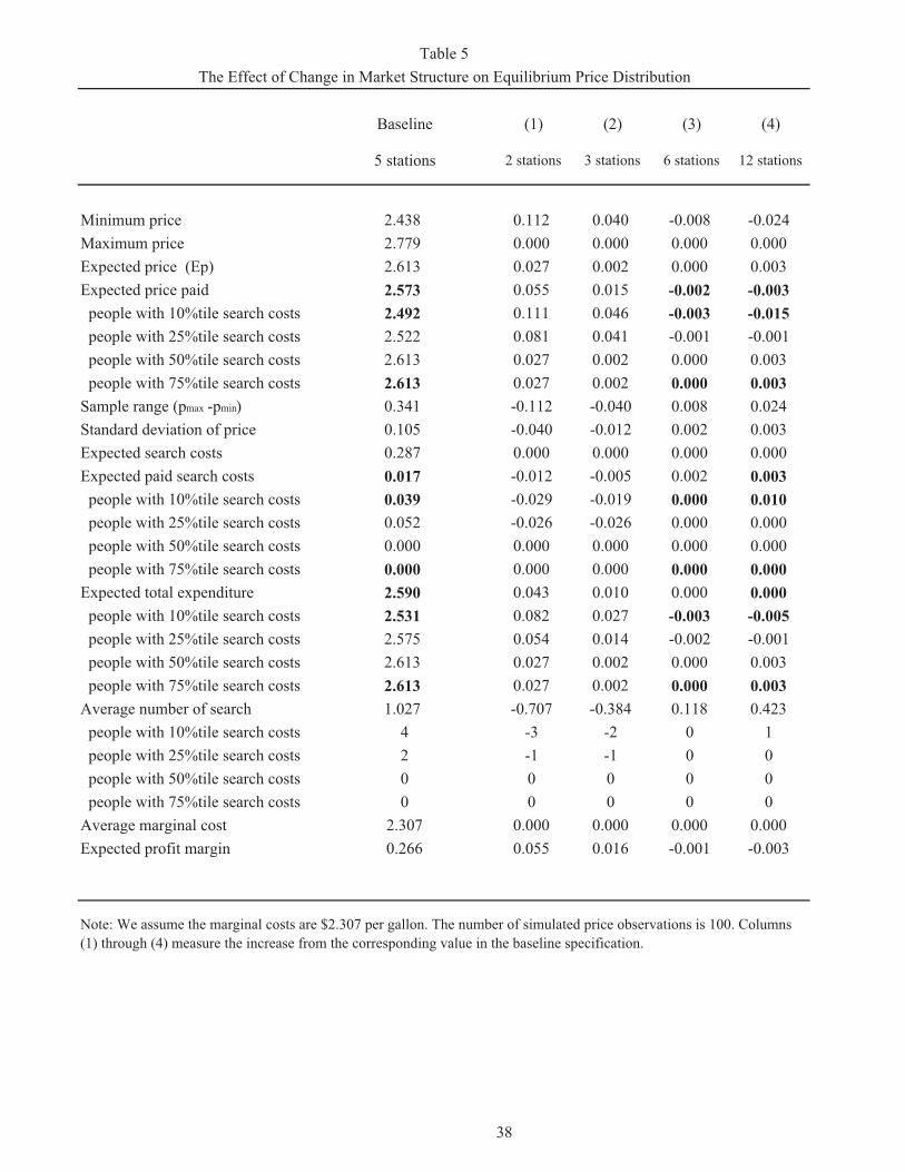
Baseline (1) (2) (3) (4)
5 stations 2 stations 3 stations 6 stations 12 stations
Minimum price 2.438 0.112 0.040 -0.008 -0.024Maximum price 2.779 0.000 0.000 0.000 0.000Expected price (Ep) 2.613 0.027 0.002 0.000 0.003Expected price paid 2.573 0.055 0.015 -0.002 -0.003 people with 10%tile search costs 2.492 0.111 0.046 -0.003 -0.015 people with 25%tile search costs 2.522 0.081 0.041 -0.001 -0.001 people with 50%tile search costs 2.613 0.027 0.002 0.000 0.003 people with 75%tile search costs 2.613 0.027 0.002 0.000 0.003Sample range (pmax -pmin) 0.341 -0.112 -0.040 0.008 0.024Standard deviation of price 0.105 -0.040 -0.012 0.002 0.003Expected search costs 0.287 0.000 0.000 0.000 0.000Expected paid search costs 0.017 -0.012 -0.005 0.002 0.003 people with 10%tile search costs 0.039 -0.029 -0.019 0.000 0.010 people with 25%tile search costs 0.052 -0.026 -0.026 0.000 0.000 people with 50%tile search costs 0.000 0.000 0.000 0.000 0.000 people with 75%tile search costs 0.000 0.000 0.000 0.000 0.000Expected total expenditure 2.590 0.043 0.010 0.000 0.000 people with 10%tile search costs 2.531 0.082 0.027 -0.003 -0.005 people with 25%tile search costs 2.575 0.054 0.014 -0.002 -0.001 people with 50%tile search costs 2.613 0.027 0.002 0.000 0.003 people with 75%tile search costs 2.613 0.027 0.002 0.000 0.003Average number of search 1.027 -0.707 -0.384 0.118 0.423 people with 10%tile search costs 4 -3 -2 0 1 people with 25%tile search costs 2 -1 -1 0 0 people with 50%tile search costs 0 0 0 0 0 people with 75%tile search costs 0 0 0 0 0Average marginal cost 2.307 0.000 0.000 0.000 0.000Expected profit margin 0.266 0.055 0.016 -0.001 -0.003
38
Table 5The Effect of Change in Market Structure on Equilibrium Price Distribution
Note: We assume the marginal costs are $2.307 per gallon. The number of simulated price observations is 100. Columns (1) through (4) measure the increase from the corresponding value in the baseline specification.

39
Figure A1
Estimated Search Costs CDF, February 27th through March 28th, 2007: All Markets
Note: The horizontal axis is the search cost per station in dollar per gallon.
Appendix Figures and Tables

40
Figure A2b
Figure A2a
Search cost cdf with 5 stations and 50% change in the expected value of search cost distribution
Simulated price distribution with 5 stations and 50 percent change in the expected value of search cost distribution
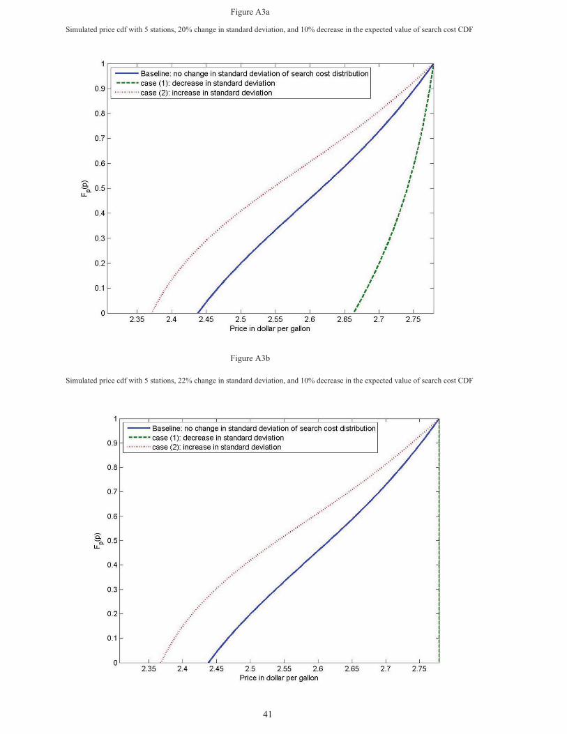
41
Figure A3a
Figure A3b
Simulated price cdf with 5 stations, 20% change in standard deviation, and 10% decrease in the expected value of search cost CDF
Simulated price cdf with 5 stations, 22% change in standard deviation, and 10% decrease in the expected value of search cost CDF

Mean Std dev Minimum Maximum
Mean household income ($) 62,270 24,700 24,328 222,764
Years of education 12.523 1.204 8.640 16.071
Age 39.035 5.407 26.489 63.419
Distance among stations (miles) 0.416 0.332 0.002 1.470
Standard Deviation of Income 47,420 12,515 18,428 117,873
42
Note: The data source is the 2006-2010 American Community Survey. The unit of observation is a single-census isolated market; there are 354 observations.
Table A1
Summary Statistics across Isolated Geographical Markets
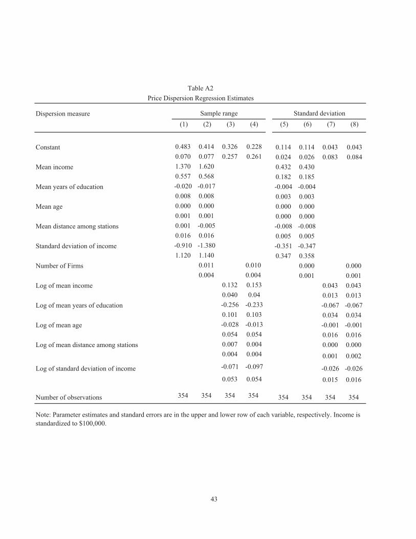
Dispersion measure(1) (2) (3) (4) (5) (6) (7) (8)
Constant 0.483 0.414 0.326 0.228 0.114 0.114 0.043 0.0430.070 0.077 0.257 0.261 0.024 0.026 0.083 0.084
Mean income 1.370 1.620 0.432 0.4300.557 0.568 0.182 0.185
Mean years of education -0.020 -0.017 -0.004 -0.0040.008 0.008 0.003 0.003
Mean age 0.000 0.000 0.000 0.0000.001 0.001 0.000 0.000
Mean distance among stations 0.001 -0.005 -0.008 -0.0080.016 0.016 0.005 0.005
Standard deviation of income -0.910 -1.380 -0.351 -0.3471.120 1.140 0.347 0.358
Number of Firms 0.011 0.010 0.000 0.0000.004 0.004 0.001 0.001
Log of mean income 0.132 0.153 0.043 0.0430.040 0.04 0.013 0.013
Log of mean years of education -0.256 -0.233 -0.067 -0.0670.101 0.103 0.034 0.034
Log of mean age -0.028 -0.013 -0.001 -0.0010.054 0.054 0.016 0.016
Log of mean distance among stations 0.007 0.004 0.000 0.0000.004 0.004 0.001 0.002
Log of standard deviation of income -0.071 -0.097 -0.026 -0.0260.053 0.054 0.015 0.016
Number of observations 354 354 354 354 354 354 354 354
43
Note: Parameter estimates and standard errors are in the upper and lower row of each variable, respectively. Income is standardized to $100,000.
Table A2Price Dispersion Regression Estimates
Sample range Standard deviation

Baseline (1) (2) (3) (4)
15% decrease 15% increase 20% decrease 20% increase
Minimum price 2.438 0.195 -0.050 0.341 -0.061Maximum price 2.779 0.000 0.000 0.000 0.000Expected price (Ep) 2.613 0.106 -0.040 0.166 -0.049Expected price paid 2.573 0.142 -0.062 0.206 -0.079 people with 10%tile search costs 2.492 0.203 -0.055 0.287 -0.068 people with 25%tile search costs 2.522 0.197 -0.073 0.257 -0.098 people with 50%tile search costs 2.613 0.106 -0.110 0.166 -0.122 people with 75%tile search costs 2.613 0.106 -0.040 0.166 -0.049Sample range (pmax -pmin) 0.341 -0.195 0.050 -0.341 0.061Standard deviation of price 0.105 -0.062 0.018 -0.105 0.023Expected search costs 0.287 0.000 0.000 0.000 0.000Expected paid search costs 0.017 -0.014 0.005 -0.017 0.006 people with 10%tile search costs 0.039 -0.020 -0.020 -0.039 -0.024 people with 25%tile search costs 0.052 -0.052 -0.008 -0.052 -0.005 people with 50%tile search costs 0 0.000 0.051 0.000 0.044 people with 75%tile search costs 0 0.000 0.000 0.000 0.000Expected total expenditure 2.590 0.128 -0.057 0.189 -0.072 people with 10%tile search costs 2.531 0.184 -0.075 0.248 -0.092 people with 25%tile search costs 2.575 0.144 -0.082 0.204 -0.103 people with 50%tile search costs 2.613 0.106 -0.059 0.166 -0.078 people with 75%tile search costs 2.613 0.106 -0.040 0.166 -0.049Average number of search 1.027 -0.774 0.484 -1.027 0.626 people with 10%tile search costs 4 -3 0 -4 0 people with 25%tile search costs 2 -2 1 -2 2 people with 50%tile search costs 0 0 1 0 1 people with 75%tile search costs 0 0 0 0 0Average marginal cost 2.307 0.000 0.000 0.000 0.000Expected profit margin 0.266 0.142 -0.062 0.206 -0.078
Proportion of people with i price quotes (qi )q1 0.564 0.304 -0.132 0.436 -0.167q2 0.154 -0.083 0.000 -0.154 -0.004q3 0.096 -0.065 0.015 -0.096 0.016q4 0.061 -0.045 0.018 -0.061 0.022q5 0.124 -0.106 0.100 -0.124 0.134
Marginal expected savings from searching i +1 versus i stations (�i )�1 0.060 -0.036 0.010 -0.060 0.012�2 0.031 -0.018 0.003 -0.031 0.004�3 0.018 -0.009 0.002 -0.018 0.002�4 0.012 -0.006 0.000 -0.012 0.000
44
Table A3The Effect of Change in Search Costs on Equilibrium Price Distribution: SOSD
Note: The number of stations is five. We assume the marginal costs are $2.307 per gallon. The number of simulated price observations is 100. Columns (1) through (4) measure the increase from the corresponding value in the baseline specification.

Table A4Summary Statistics of Simulated Equilibrium Pices by Market Structure
# of stations
Minimumprice
Expectedprice
Expectedprice paid
SampleRange
Standarddeviation of
prices
Expectedsearch
costs paid
Totalexpenditure
Gains from search
2 2.549740 2.639609 2.627892 0.229260 0.065354 0.005347 2.633239 0.0898693 2.477898 2.615278 2.588151 0.301102 0.092603 0.011918 2.600070 0.1373804 2.451537 2.612354 2.577110 0.327463 0.101622 0.015448 2.592558 0.1608165 2.438109 2.612645 2.573076 0.340891 0.105213 0.017396 2.590472 0.1745366 2.430114 2.613401 2.571410 0.348886 0.106802 0.018524 2.589934 0.1832877 2.424906 2.614084 2.570673 0.354094 0.107555 0.019206 2.589879 0.1891788 2.421313 2.614610 2.570336 0.357687 0.107928 0.019632 2.589968 0.1932989 2.418730 2.614996 2.570179 0.360270 0.108118 0.019907 2.590086 0.196265
10 2.416819 2.615274 2.570108 0.362181 0.108218 0.020087 2.590196 0.19845511 2.415371 2.615475 2.570077 0.363629 0.108270 0.020208 2.590285 0.20010412 2.414253 2.615620 2.570067 0.364747 0.108298 0.020292 2.590359 0.20136713 2.413377 2.615726 2.570064 0.365623 0.108313 0.020352 2.590416 0.20235014 2.412683 2.615804 2.570068 0.366317 0.108320 0.020394 2.590461 0.20312115 2.412125 2.615863 2.570073 0.366875 0.108323 0.020424 2.590497 0.20373716 2.411674 2.615906 2.570079 0.367326 0.108324 0.020446 2.590524 0.20423217 2.411304 2.615940 2.570084 0.367696 0.108325 0.020462 2.590546 0.20463618 2.411000 2.615965 2.570089 0.368000 0.108324 0.020474 2.590563 0.20496519 2.410747 2.615985 2.570092 0.368253 0.108325 0.020484 2.590576 0.20523820 2.410536 2.616000 2.570095 0.368464 0.108324 0.020491 2.590587 0.20546421 2.410359 2.616012 2.570098 0.368641 0.108324 0.020497 2.590595 0.20565322 2.410210 2.616019 2.570097 0.368790 0.108324 0.020501 2.590599 0.20580923 2.410082 2.616026 2.570099 0.368918 0.108323 0.020505 2.590604 0.20594424 2.409975 2.616031 2.570100 0.369025 0.108323 0.020507 2.590608 0.20605625 2.409882 2.616036 2.570101 0.369118 0.108323 0.020510 2.590611 0.20615326 2.409803 2.616039 2.570102 0.369197 0.108323 0.020511 2.590613 0.20623727 2.409734 2.616042 2.570103 0.369266 0.108323 0.020513 2.590616 0.20630828 2.409674 2.616045 2.570104 0.369326 0.108323 0.020514 2.590617 0.20637029 2.409623 2.616047 2.570104 0.369377 0.108322 0.020515 2.590619 0.20642430 2.409578 2.616048 2.570105 0.369422 0.108322 0.020515 2.590621 0.206470
Note: The unit is dollar per gallon.
45


