1
Lecture 4:
Sampling of Continuous-Time Signals
Reza Mohammadkhani, Digital Signal Processing, 2014University of Kurdistan eng.uok.ac.ir/mohammadkhani
Signal Types2
� Analog signals: continuous in time and amplitude
� Digital signals: discrete both in time and amplitude
� Discrete-time signals: discrete in time, continuous in amplitude
� Theory for digital signals would be too complicated� Requires inclusion of nonlinearities into theory
� Theory is based on discrete-time continuous-amplitude signals� Most convenient to develop theory
� Good enough approximation to practice with some care
� In practice we mostly process digital signals on processors� Need to take into account finite precision effects
Part 1: Periodic Sampling3
� Periodic sampling
� Frequency domain representation
� Reconstruction
� Discrete-Time Processing of Continuous-Time Signals
� Changing the sampling rate of discrete-time signals
Periodic (Uniform) Sampling4
� Sampling is a continuous to discrete-time conversion
� Most common sampling is periodic:
�[�] = ��(�)
where is the sampling period in second,
�� = 1/ is the sampling frequency in Hz, and
Ω� = 2π�� is sampling frequency in radian-per-second
� Use ⋅ for discrete-time and ⋅ for continuous time signals
� This is the ideal case not the practical but close enough
� In practice it is implement with an analog-to-digital converters
� We get digital signals that are quantized in amplitude and time
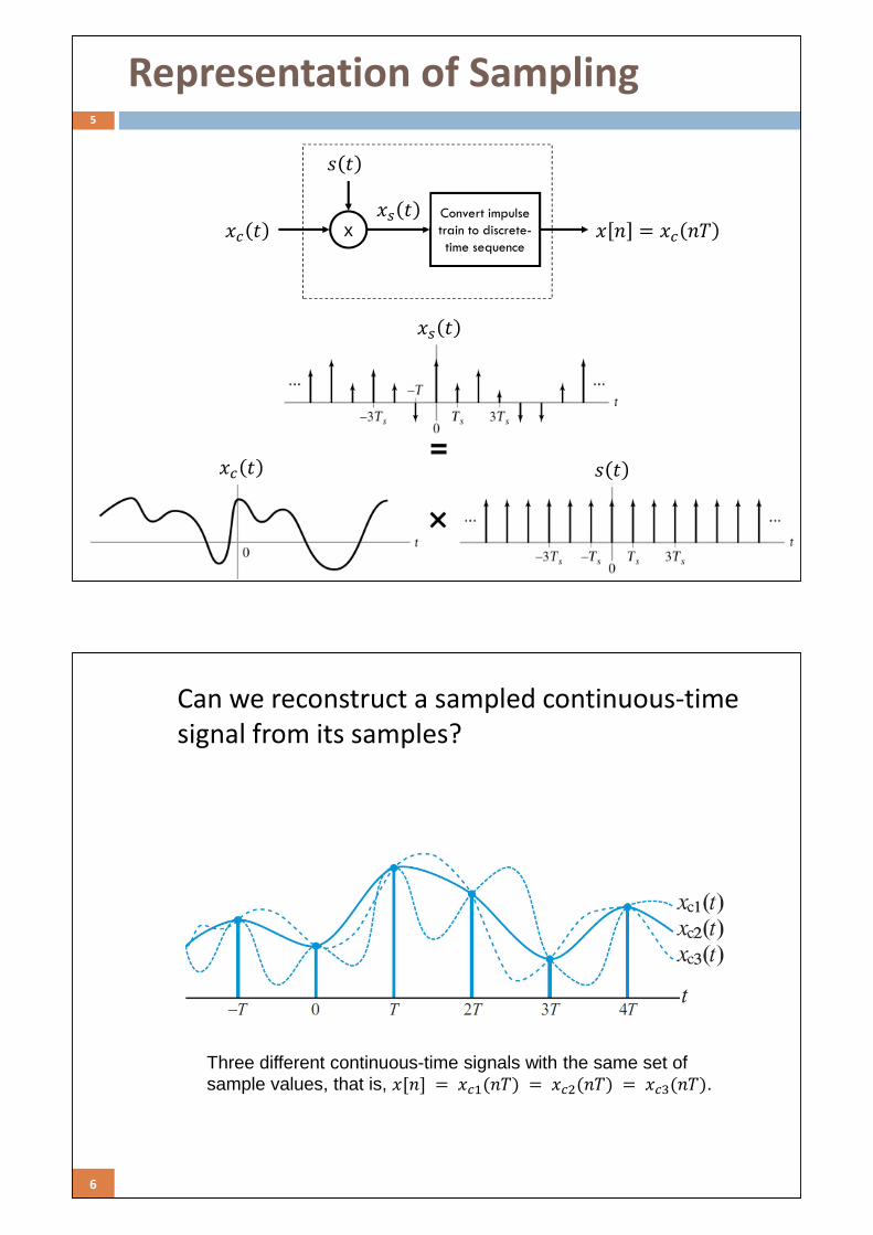
Representation of Sampling5
Convert impulse
train to discrete-
time sequence�� � � � = �� �x
� �
� ��� �
�� �
�� �
6
Can we reconstruct a sampled continuous-time
signal from its samples?
Three different continuous-time signals with the same set of sample values, that is, �[�] � ����� � ����� � �����.
7
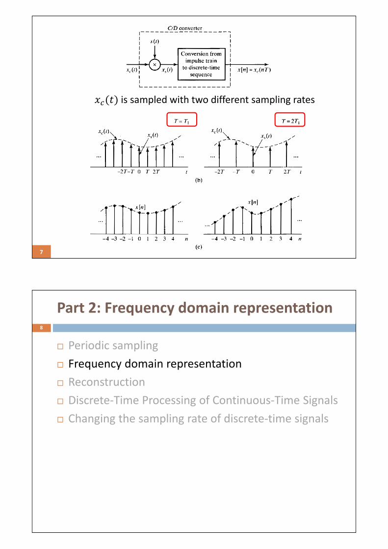
����is sampled with two different sampling rates
Part 2: Frequency domain representation8
� Periodic sampling
� Frequency domain representation
� Reconstruction
� Discrete-Time Processing of Continuous-Time Signals
� Changing the sampling rate of discrete-time signals
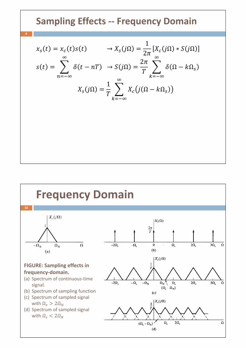
Sampling Effects -- Frequency Domain9
�� � � �� � � � → �� �Ω =1
2� �� �Ω ∗ � �Ω
� � � � � � − �
!"# → � �Ω =
2� � � Ω − $Ω�
%"#
�� �Ω �1 � �� � Ω − $Ω�
%"#
Frequency Domain10
FIGURE: Sampling effects in
frequency-domain.
(a) Spectrum of continuous-time
signal.
(b) Spectrum of sampling function
(c) Spectrum of sampled signal
with Ω� & 2Ω'(d) Spectrum of sampled signal
with (� ) 2('
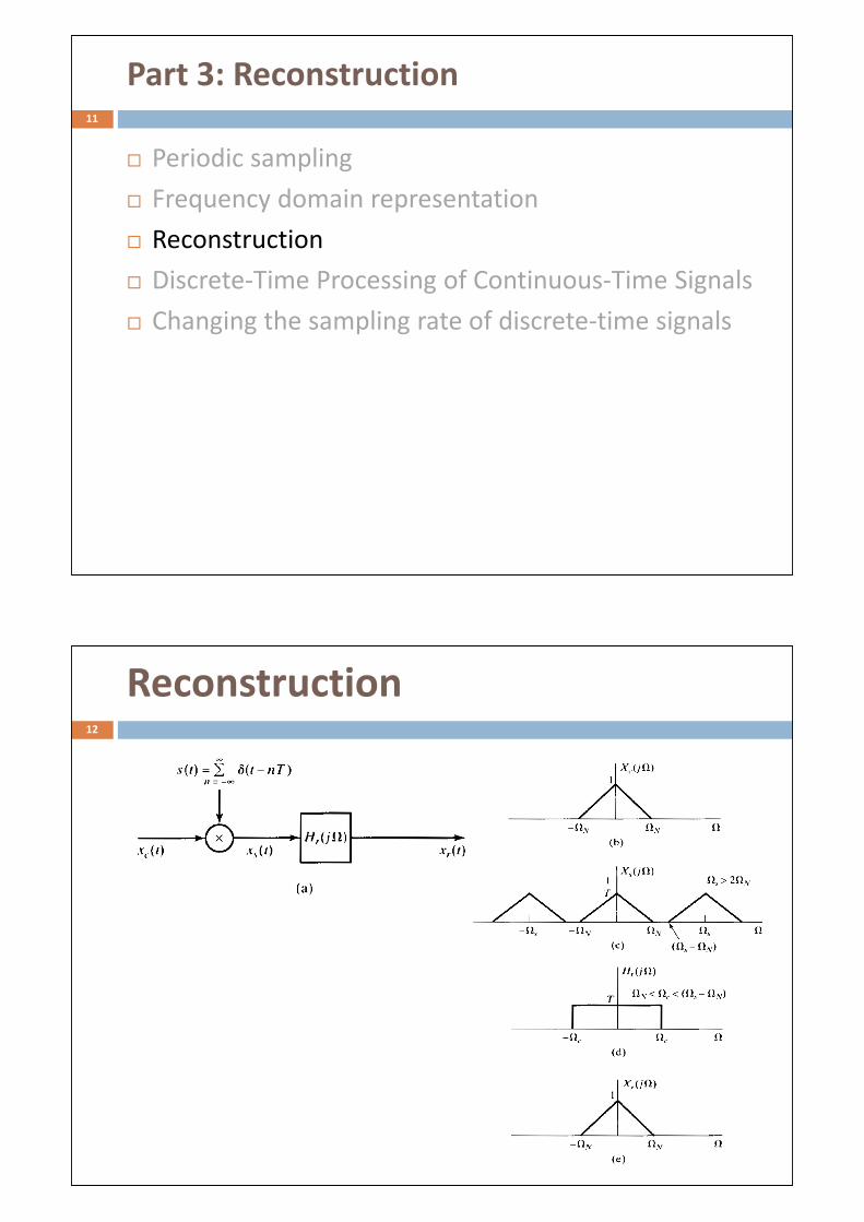
Part 3: Reconstruction11
� Periodic sampling
� Frequency domain representation
� Reconstruction
� Discrete-Time Processing of Continuous-Time Signals
� Changing the sampling rate of discrete-time signals
Reconstruction12
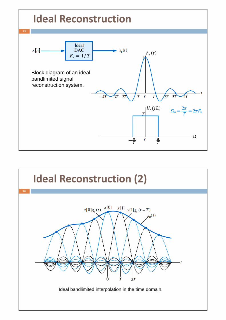
Ideal Reconstruction13
*+ �
,+��Ω
Block diagram of an ideal bandlimited signal reconstruction system.
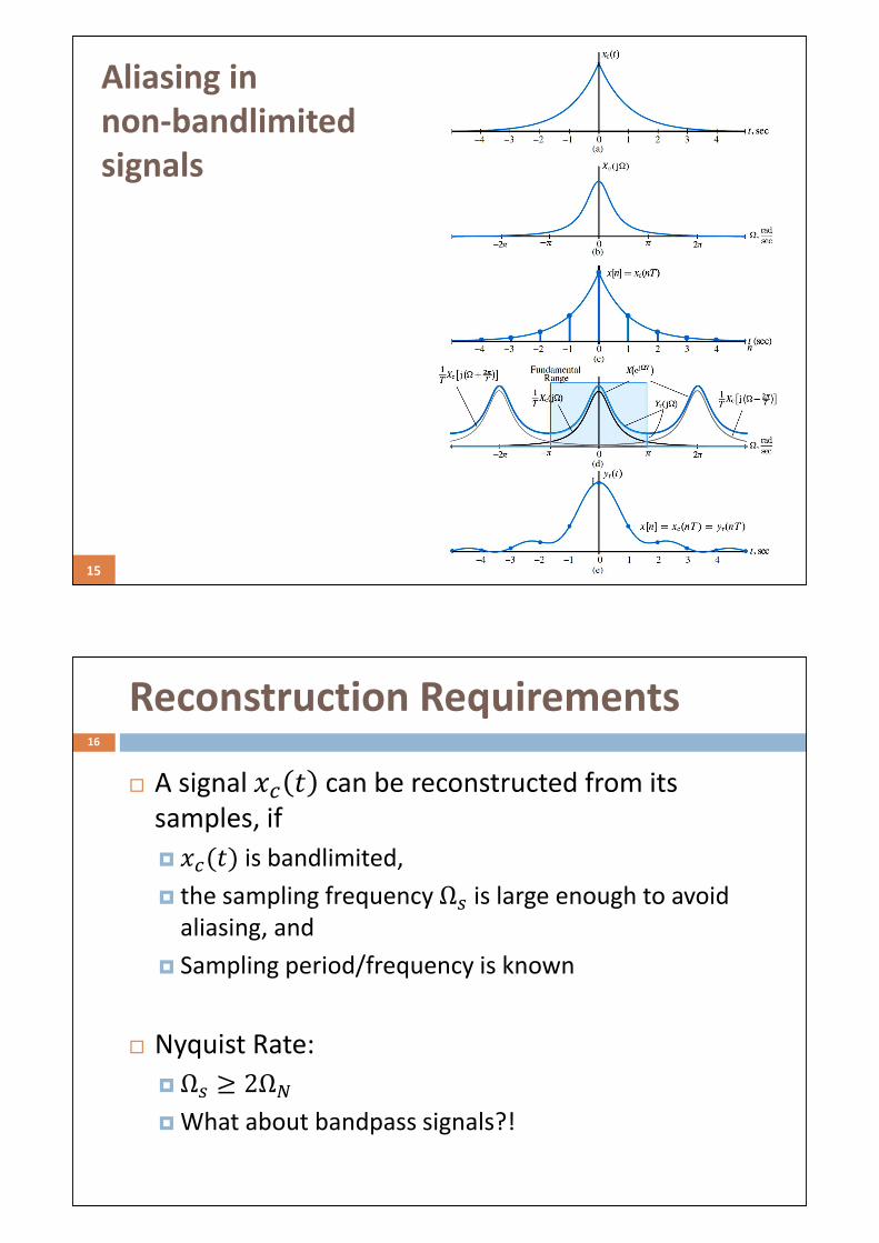
Ideal Reconstruction (2)14
Ideal bandlimited interpolation in the time domain.
15
Aliasing in
non-bandlimited
signals
Reconstruction Requirements16
� A signal �� � can be reconstructed from its
samples, if
� ��(� is bandlimited,
� the sampling frequency Ω� is large enough to avoid
aliasing, and
� Sampling period/frequency is known
� Nyquist Rate:
� Ω� ≥ 2Ω'
� What about bandpass signals?!
Part 4:
Discrete-Time Processing of Continuous-Time Signals17
� Periodic sampling
� Frequency domain representation
� Reconstruction
� Discrete-Time Processing of Continuous-Time Signals
� Changing the sampling rate of discrete-time signals
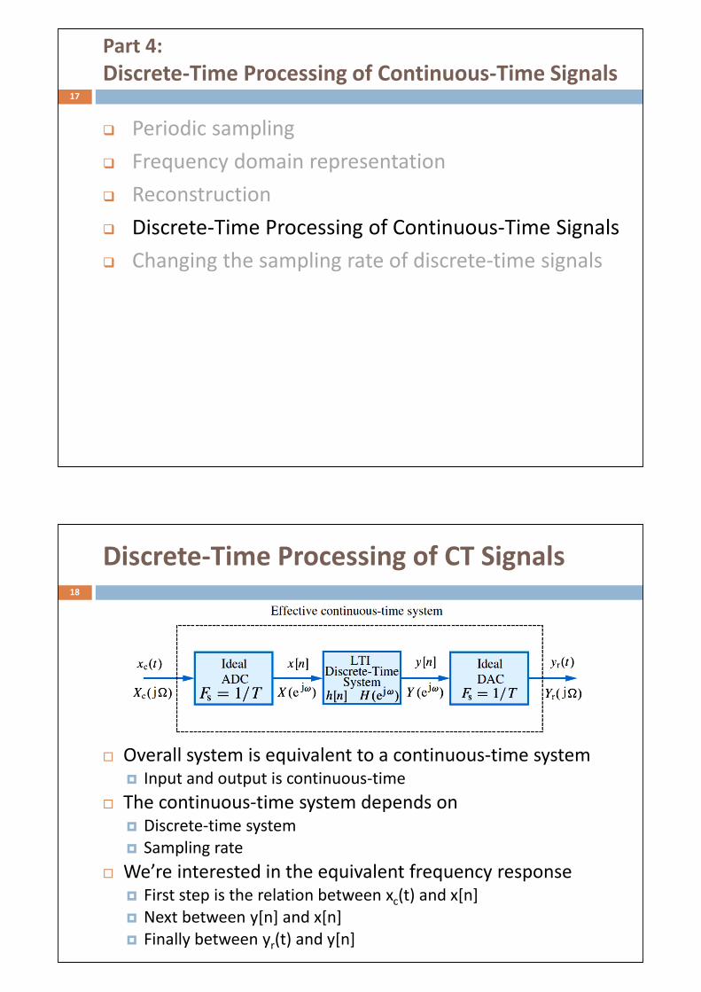
Discrete-Time Processing of CT Signals18
� Overall system is equivalent to a continuous-time system� Input and output is continuous-time
� The continuous-time system depends on� Discrete-time system
� Sampling rate
� We’re interested in the equivalent frequency response � First step is the relation between xc(t) and x[n]
� Next between y[n] and x[n]
� Finally between yr(t) and y[n]

LTI Discrete-Time System19
� Input:
� � � � �� � � ./0 10"23 ��3∑ �� �Ω � � �5
3 $ %"# � � � 6
3
� Output of LTI system
� 7 � � * � ∗ � � → 8 ./0 � , ./0 � ./0� Output DT to CT
� 8+ �Ω � 9:; �Ω 8 ./23
� 8+ �Ω � 9:; �Ω , ./23 � ./23
� � 9:; �Ω , ./23 �3 ∑ �� �Ω � � �5
3 $ %"#
� � < Ω < �
8+ �Ω � ,=>> �Ω �� �Ω
20
Part 5:
Changing the sampling rate of discrete-time signals21
� Periodic sampling
� Frequency domain representation
� Reconstruction
� Discrete-Time Processing of Continuous-Time Signals
� Changing the sampling rate of discrete-time signals
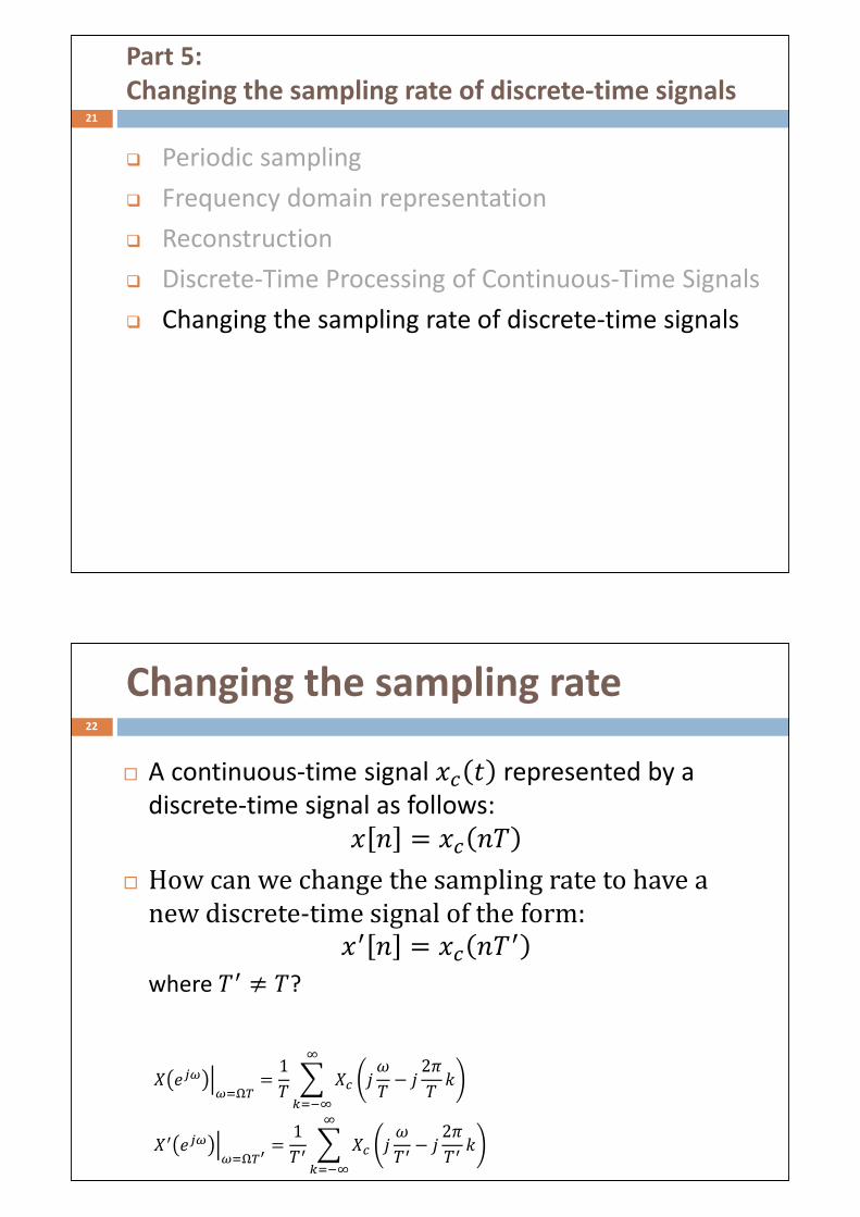
Changing the sampling rate 22
� A continuous-time signal �� � represented by a
discrete-time signal as follows:
� � � �� �� How can we change the sampling rate to have a
new discrete-time signal of the form:�T � � �� �T
where T ≠ ?
� ./0 V0"23 � 1 � �� � W
� � 2� $
%"#
�T ./0 V0"23X � 1T � �� � W
T � � 2�T $
%"#

Downsampling23
� Downsampling
� �Y � � � �Z � �� �Z
Downsampling24
� To avoid aliasing in downsampling by a factor of M
requires that:
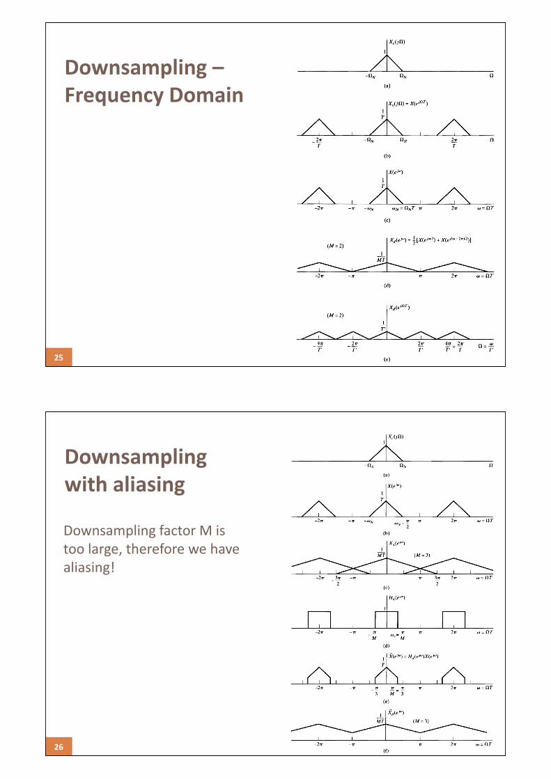
25
Downsampling –
Frequency Domain
26
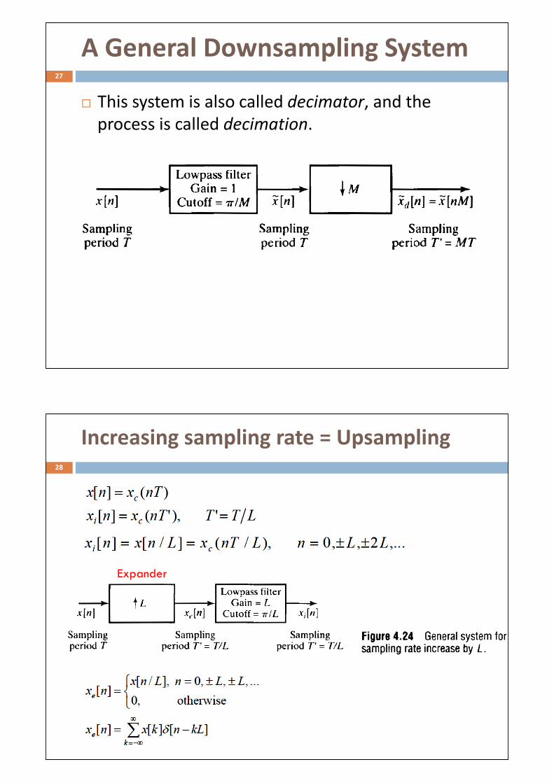
Downsampling
with aliasing
Downsampling factor M is
too large, therefore we have
aliasing!
A General Downsampling System27
� This system is also called decimator, and the
process is called decimation.
Increasing sampling rate = Upsampling
28
Expander
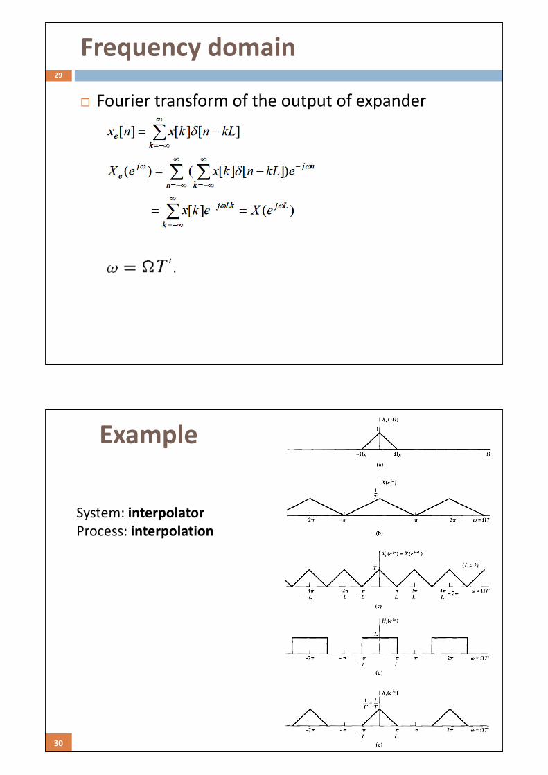
Frequency domain29
� Fourier transform of the output of expander
30
Example
System: interpolator
Process: interpolation
31
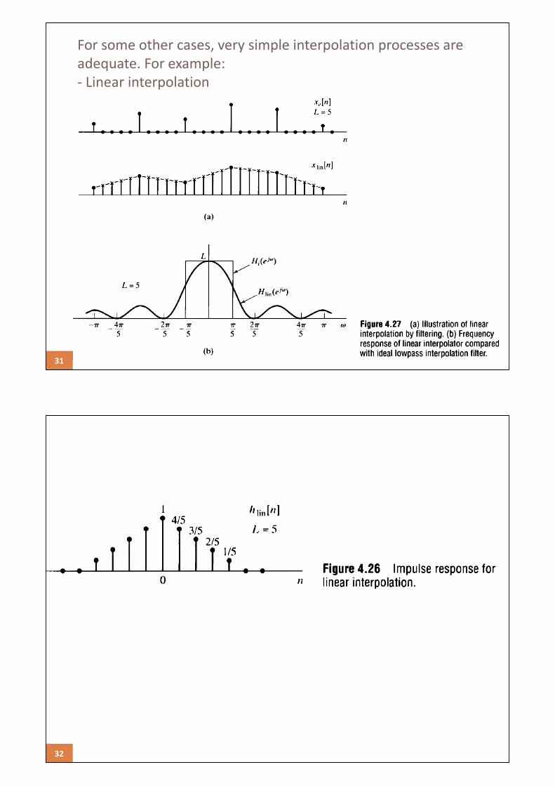
For some other cases, very simple interpolation processes are
adequate. For example:
- Linear interpolation
32
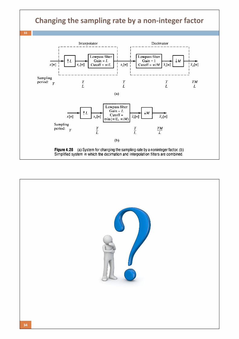
Changing the sampling rate by a non-integer factor
33
34
References35
� A. V. Oppenheim and R. W. Schafer, Discrete-Time
Signal Processing, 3rd Edition, Prentice Hall, 2009.
� D. Manolakis and V. Ingle, Applied Digital Signal
Processing, Cambridge University Press, 2011.
� Miki Lustig, EE123 Digital Signal Processing, Lecture
notes, Electrical Engineering and Computer Science,
UC Berkeley, CA, 2012. Available at:http://inst.eecs.berkeley.edu/~ee123/fa12/


