Download - Routing Protocol Review
1
Routing Protocol Review
(some slides borrowed from Eugene Ng @ Rice Univ.)
2
Internet Routing
AS 73AS 9
AS 5050
AS 4554AS 101
AS 3999
Internet
3
Routing Protocol Review
Part 1: Intra-domain routing

4
Intra-domain Routing Protocols
• Two intra-domain routing protocols• Both try to achieve the “shortest path” forwarding• Quite commonly used
• OSPF: Based on Link-State routing algorithm• RIP: Based on Distance-Vector routing algorithm
• In Project 2, you implemented and played around with OSPF!

5
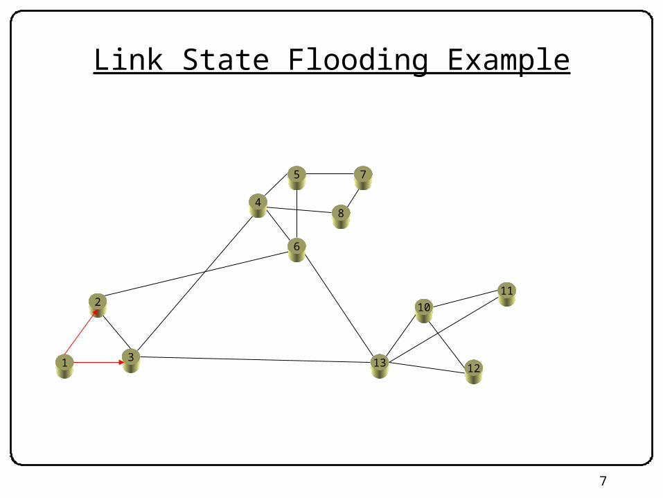
Link State Routing (OSPF): Flooding
• Each node knows its connectivity and cost to a direct neighbor
• Every node tells every other node this local connectivity/cost information– Via flooding
• In the end, every node learns the complete topology of the network
• E.g. A floods messageA
ED
CB
F
2
2
13
1
1
2
53
5
A connected to B cost 2A connected to D cost 1A connected to C cost 5
6
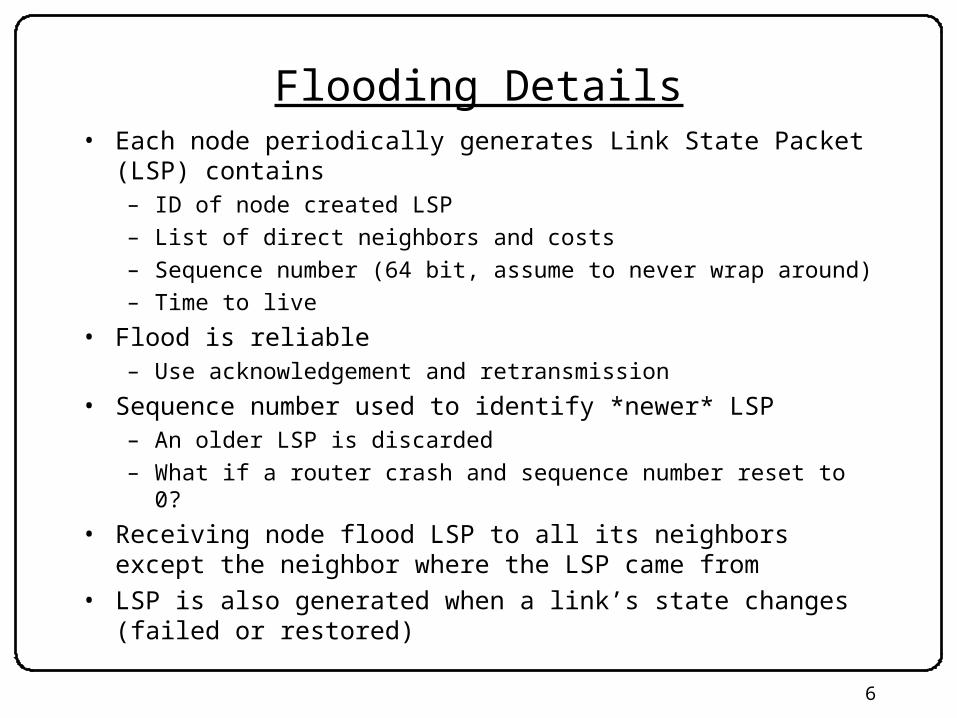
Flooding Details• Each node periodically generates Link State Packet (LSP)
contains– ID of node created LSP
– List of direct neighbors and costs
– Sequence number (64 bit, assume to never wrap around)
– Time to live
• Flood is reliable– Use acknowledgement and retransmission
• Sequence number used to identify *newer* LSP– An older LSP is discarded
– What if a router crash and sequence number reset to 0?
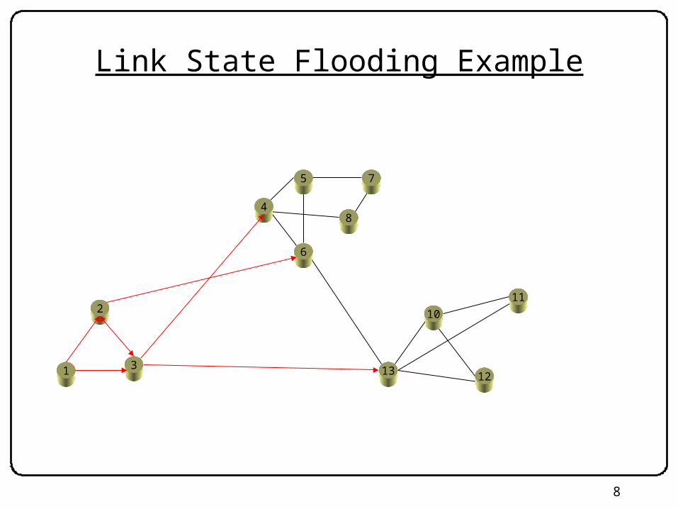
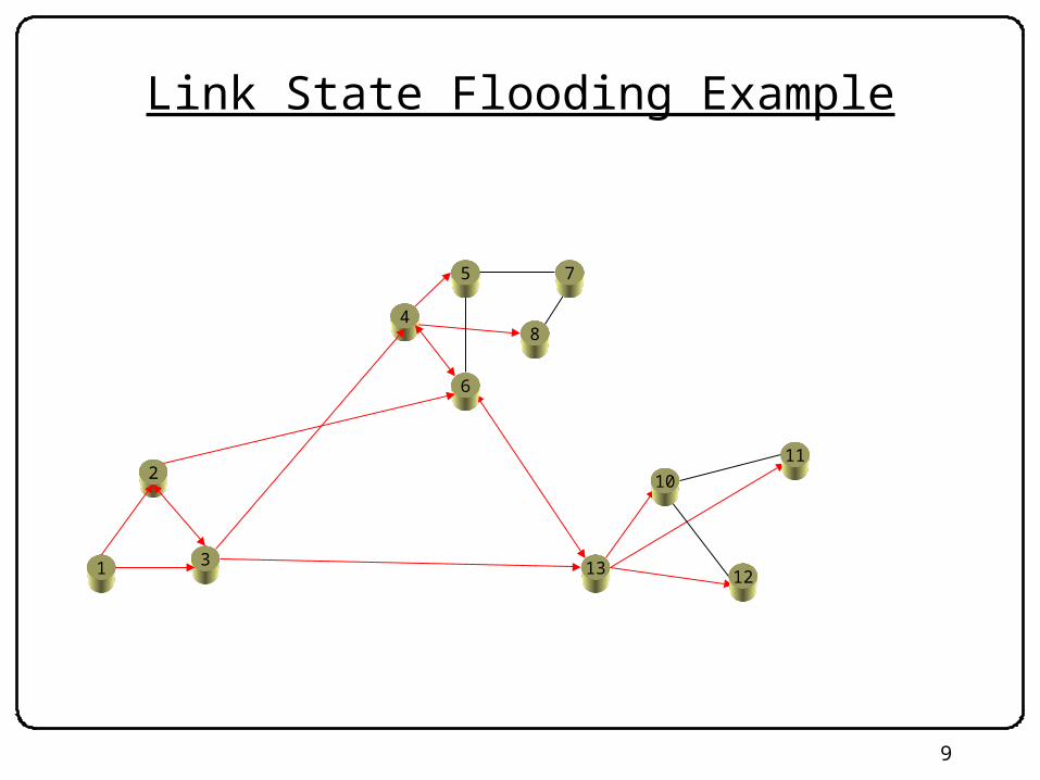
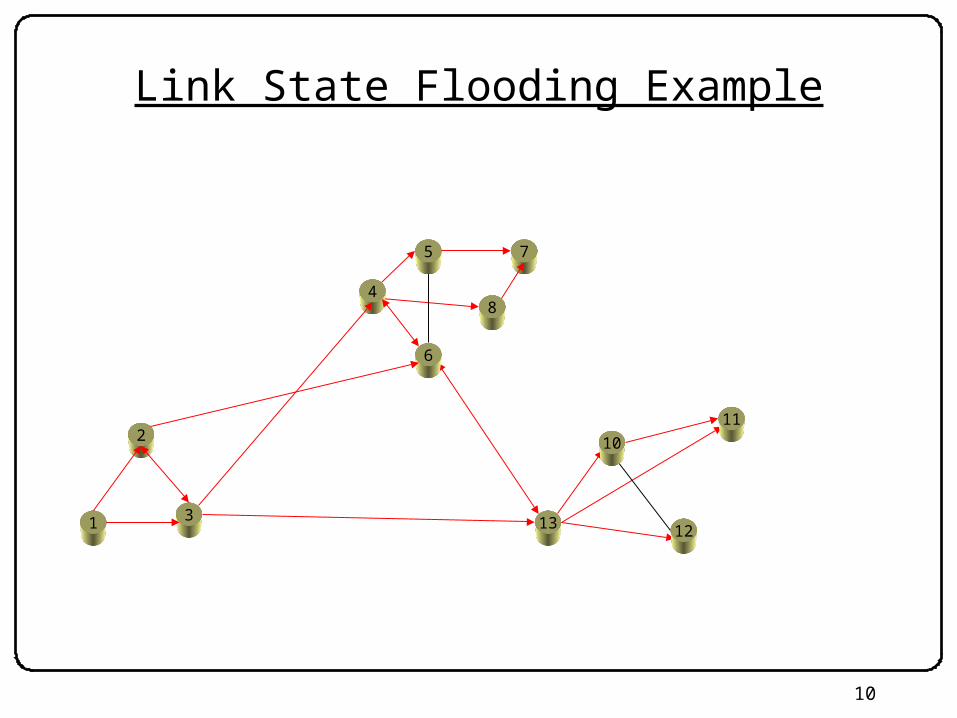
• Receiving node flood LSP to all its neighbors except the neighbor where the LSP came from
• LSP is also generated when a link’s state changes (failed or restored)
7
Link State Flooding Example
6
7
8
5
4
31
2
12
10
13
11
8
Link State Flooding Example
6
7
8
5
4
31
2
12
10
13
11
9
Link State Flooding Example
6
7
8
5
4
31
2
12
10
13
11
10
Link State Flooding Example
6
7
8
5
4
31
2
12
10
13
11

11
A Link State Routing Algorithm
Dijkstra’s algorithm• Net topology, link costs known
to all nodes– Accomplished via “link state
flooding” – All nodes have same info
• Compute least cost paths from one node (‘source”) to all other nodes
• Repeat for all sources
Notations• c(i,j): link cost from node i to
j; cost infinite if not direct neighbors
• D(v): current value of cost of path from source to node v
• p(v): predecessor node along path from source to v, that is next to v
• S: set of nodes whose least cost path definitively known

12
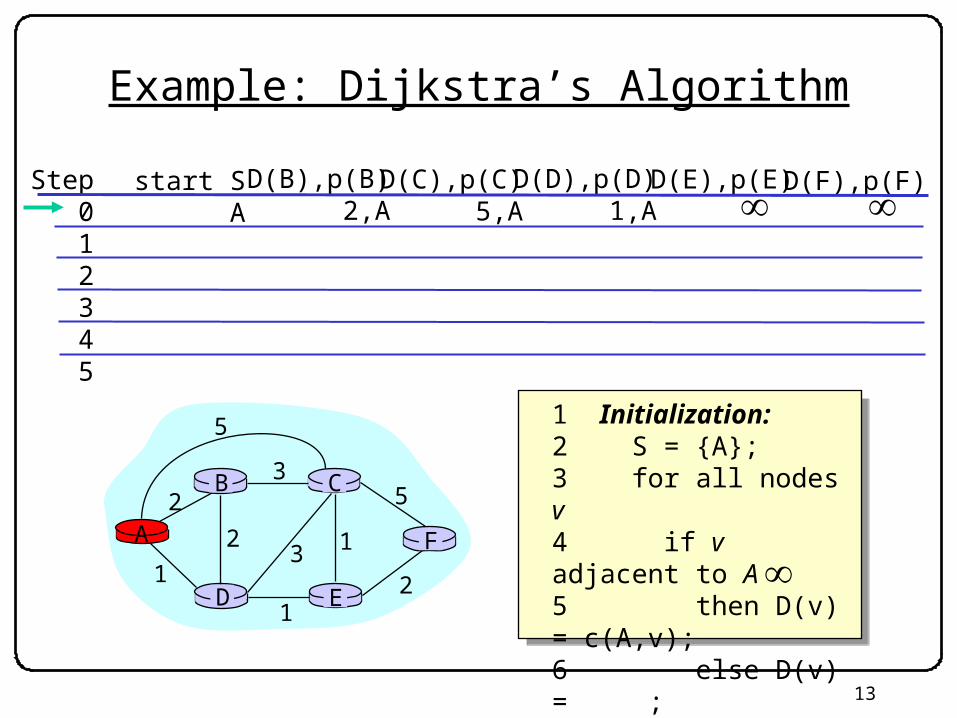
Dijsktra’s Algorithm (A “Greedy” Algorithm)
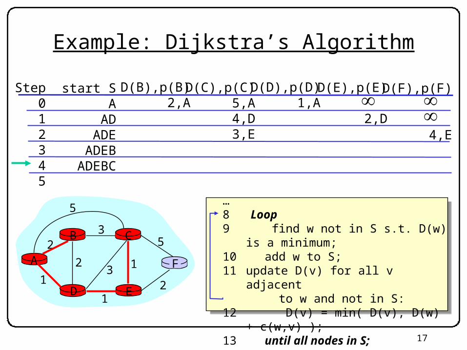
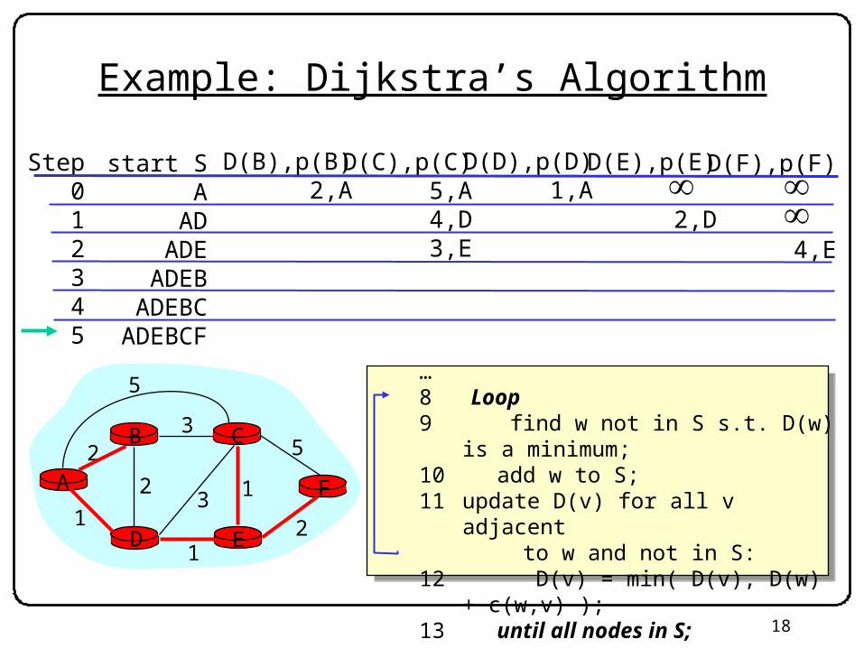
1 Initialization: 2 S = {A};3 for all nodes v 4 if v adjacent to A 5 then D(v) = c(A,v); 6 else D(v) = ;7 8 Loop 9 find w not in S such that D(w) is a minimum; 10 add w to S; 11 update D(v) for all v adjacent to w and not in S: 12 D(v) = min( D(v), D(w) + c(w,v) ); // new cost to v is either old cost to v or known // shortest path cost to w plus cost from w to v 13 until all nodes in S;
13
Example: Dijkstra’s Algorithm
Step012345
start SA
D(B),p(B)2,A
D(C),p(C)5,A
D(D),p(D)1,A
D(E),p(E) D(F),p(F)
A
ED
CB
F
2
2
13
1
1
2
53
5
1 Initialization: 2 S = {A};3 for all nodes v 4 if v adjacent to A 5 then D(v) = c(A,v); 6 else D(v) = ;…
14
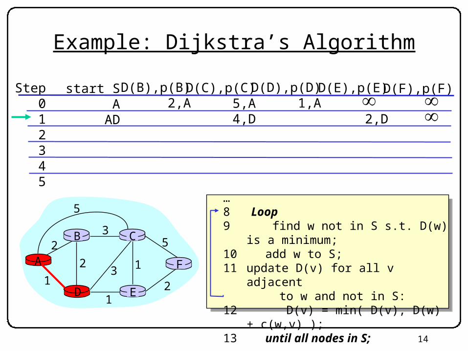
Example: Dijkstra’s Algorithm
Step012345
start SA
AD
D(B),p(B)2,A
D(C),p(C)5,A4,D
D(D),p(D)1,A
D(E),p(E)
2,D
D(F),p(F)
A
ED
CB
F
2
2
13
1
1
2
53
5
…8 Loop 9 find w not in S s.t. D(w) is a minimum; 10 add w to S; 11 update D(v) for all v adjacent to w and not in S: 12 D(v) = min( D(v), D(w) + c(w,v) );13 until all nodes in S;
15
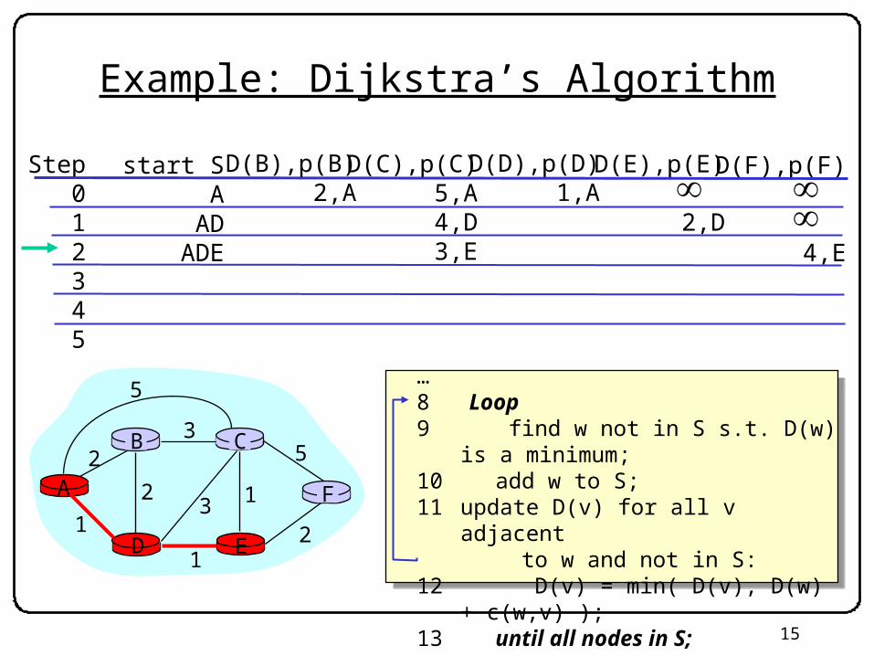
Example: Dijkstra’s Algorithm
Step012345
start SA
ADADE
D(B),p(B)2,A
D(C),p(C)5,A4,D3,E
D(D),p(D)1,A
D(E),p(E)
2,D
D(F),p(F)
4,E
A
ED
CB
F
2
2
13
1
1
2
53
5…8 Loop 9 find w not in S s.t. D(w) is a minimum; 10 add w to S; 11 update D(v) for all v adjacent to w and not in S: 12 D(v) = min( D(v), D(w) + c(w,v) );13 until all nodes in S;
16
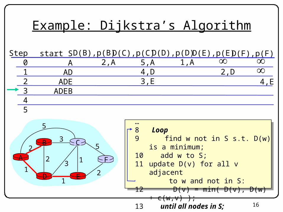
Example: Dijkstra’s Algorithm
Step012345
start SA
ADADE
ADEB
D(B),p(B)2,A
D(C),p(C)5,A4,D3,E
D(D),p(D)1,A
D(E),p(E)
2,D
D(F),p(F)
4,E
A
ED
CB
F
2
2
13
1
1
2
53
5…8 Loop 9 find w not in S s.t. D(w) is a minimum; 10 add w to S; 11 update D(v) for all v adjacent to w and not in S: 12 D(v) = min( D(v), D(w) + c(w,v) );13 until all nodes in S;
17
Example: Dijkstra’s Algorithm
Step012345
start SA
ADADE
ADEBADEBC
D(B),p(B)2,A
D(C),p(C)5,A4,D3,E
D(D),p(D)1,A
D(E),p(E)
2,D
D(F),p(F)
4,E
A
ED
CB
F
2
2
13
1
1
2
53
5…8 Loop 9 find w not in S s.t. D(w) is a minimum; 10 add w to S; 11 update D(v) for all v adjacent to w and not in S: 12 D(v) = min( D(v), D(w) + c(w,v) );13 until all nodes in S;
18
Example: Dijkstra’s Algorithm
Step012345
start SA
ADADE
ADEBADEBC
ADEBCF
D(B),p(B)2,A
D(C),p(C)5,A4,D3,E
D(D),p(D)1,A
D(E),p(E)
2,D
D(F),p(F)
4,E
A
ED
CB
F
2
2
13
1
1
2
53
5…8 Loop 9 find w not in S s.t. D(w) is a minimum; 10 add w to S; 11 update D(v) for all v adjacent to w and not in S: 12 D(v) = min( D(v), D(w) + c(w,v) );13 until all nodes in S;

19
Distance Vector Routing (RIP)
• What is a distance vector?– Current best known cost to get to a destination
• Idea: Exchange distance vectors among neighbors to learn about lowest cost paths
Dest. Cost
A 7
B 1
D 2
E 5
F 1
G 3
Node C
Note no vector entry for C itself
At the beginning, distance vector only has information about directly attached neighbors, all other dests
have cost
Eventually the vector is filled
20
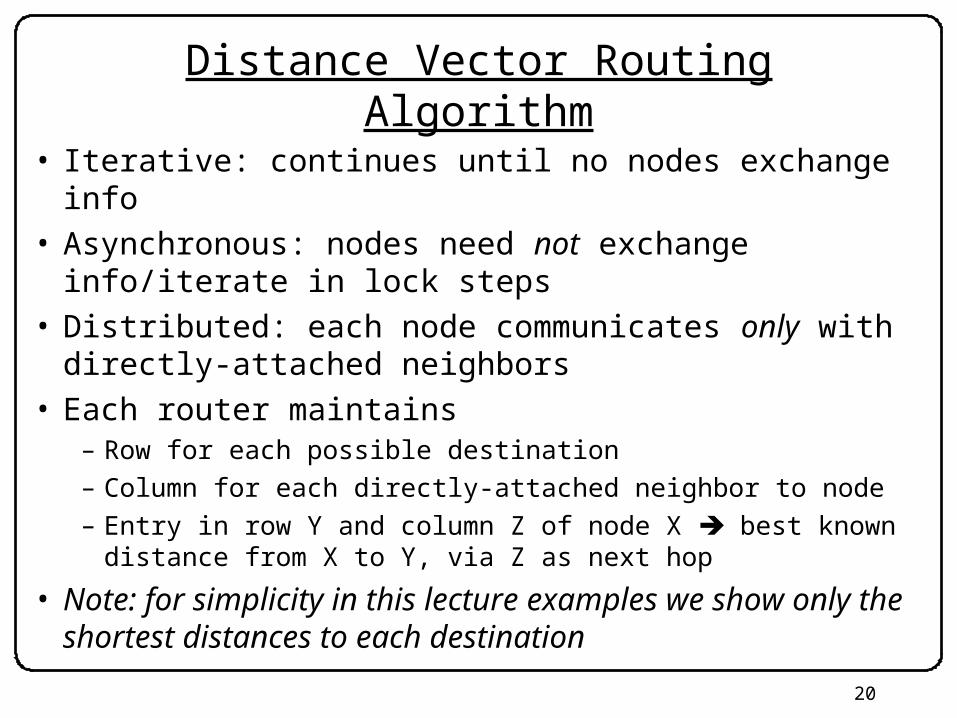
Distance Vector Routing Algorithm
• Iterative: continues until no nodes exchange info• Asynchronous: nodes need not exchange info/iterate in lock
steps• Distributed: each node communicates only with directly-
attached neighbors• Each router maintains
– Row for each possible destination– Column for each directly-attached neighbor to node– Entry in row Y and column Z of node X best known distance from X
to Y, via Z as next hop
• Note: for simplicity in this lecture examples we show only the shortest distances to each destination
21
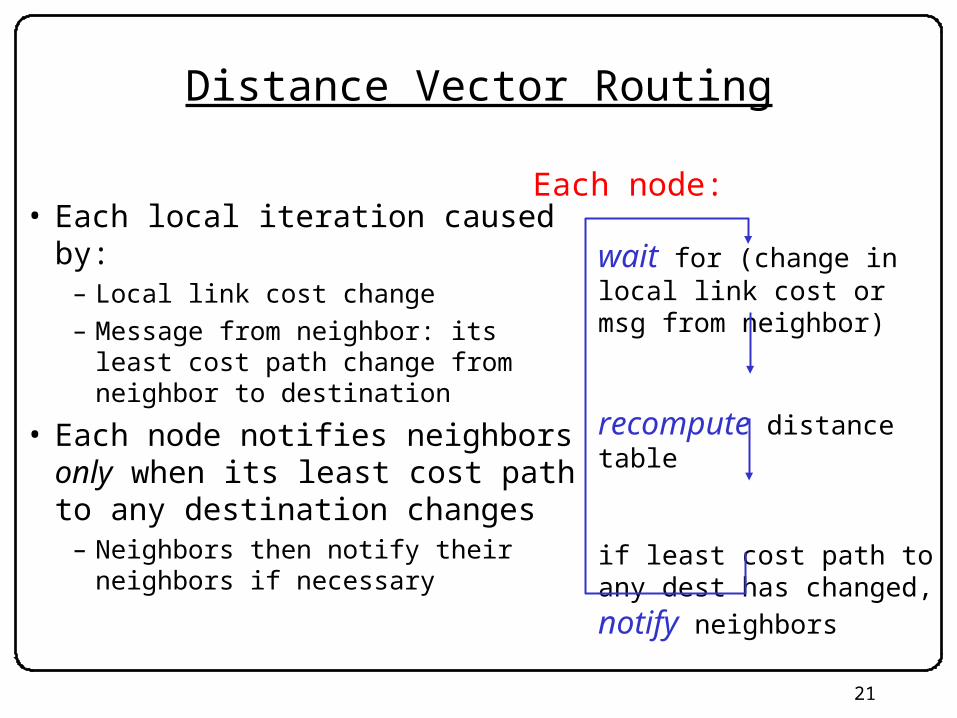
Distance Vector Routing
• Each local iteration caused by: – Local link cost change – Message from neighbor: its least cost
path change from neighbor to destination
• Each node notifies neighbors only when its least cost path to any destination changes
– Neighbors then notify their neighbors if necessary
wait for (change in local link cost or msg from neighbor)
recompute distance table
if least cost path to any dest
has changed, notify neighbors
Each node:
22
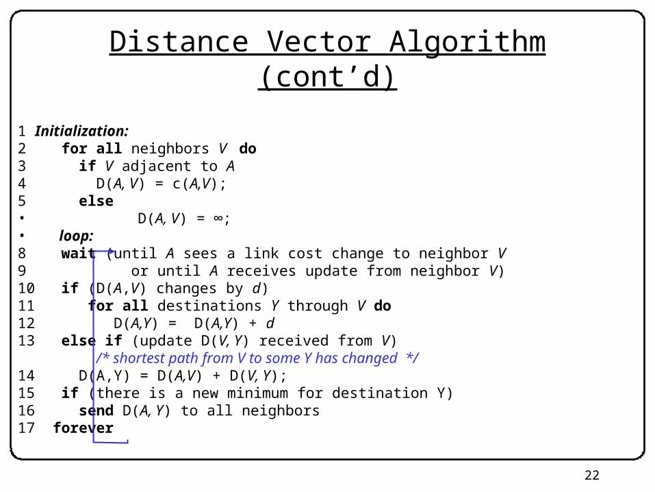
Distance Vector Algorithm (cont’d)
1 Initialization: 2 for all neighbors V do3 if V adjacent to A 4 D(A, V) = c(A,V); 5 else • D(A, V) = ∞; • loop: 8 wait (until A sees a link cost change to neighbor V 9 or until A receives update from neighbor V) 10 if (D(A,V) changes by d) 11 for all destinations Y through V do 12 D(A,Y) = D(A,Y) + d 13 else if (update D(V, Y) received from V) /* shortest path from V to some Y has changed */ 14 D(A,Y) = D(A,V) + D(V, Y);15 if (there is a new minimum for destination Y)16 send D(A, Y) to all neighbors 17 forever
23
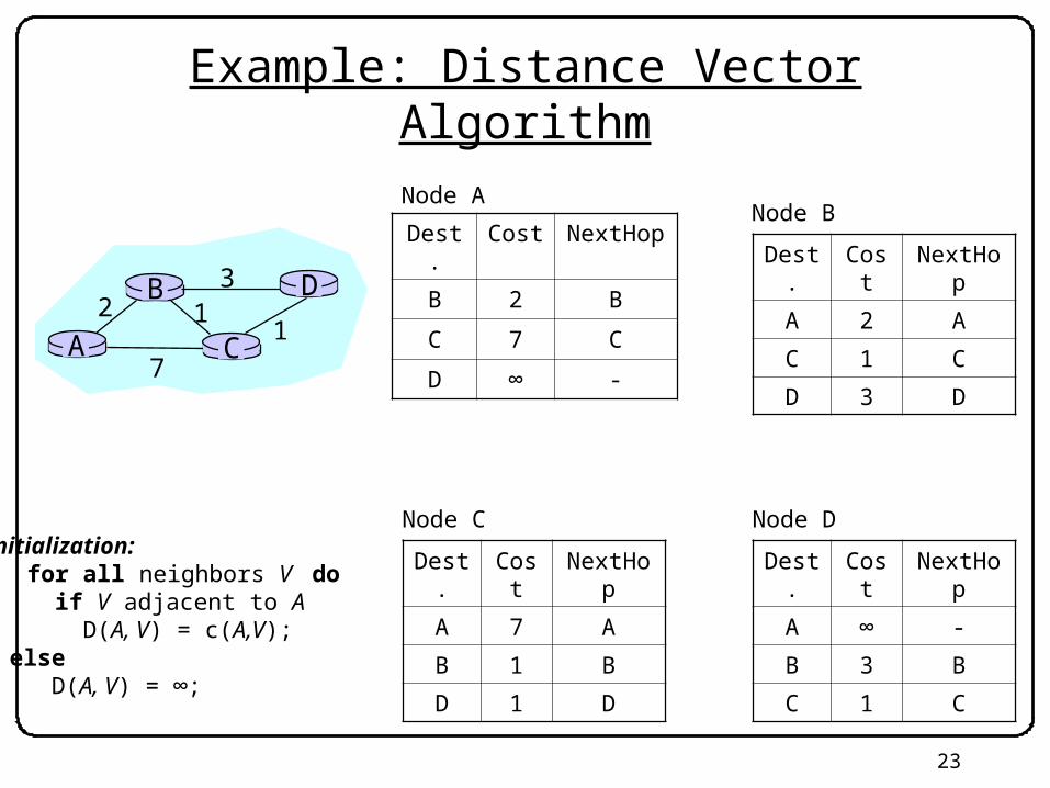
Example: Distance Vector Algorithm
A C12
7
B D3
1
Dest. Cost NextHop
B 2 B
C 7 C
D ∞ -
Node A
Dest. Cost NextHop
A 2 A
C 1 C
D 3 D
Node B
Dest. Cost NextHop
A 7 A
B 1 B
D 1 D
Node C
Dest. Cost NextHop
A ∞ -
B 3 B
C 1 C
Node D1 Initialization: 2 for all neighbors V do3 if V adjacent to A 4 D(A, V) = c(A,V); 5 else 6 D(A, V) = ∞; …

24
Dest. Cost NextHop
B 2 B
C 7 C
D 8 C
Node A
Example: 1st Iteration (C A)
A C12
7
B D3
1Dest. Cost NextHop
A 2 A
C 1 C
D 3 D
Node B
Dest. Cost NextHop
A 7 A
B 1 B
D 1 D
Node C
Dest. Cost NextHop
A ∞ -
B 3 B
C 1 C
Node D
D(A, D) = D(A, C) + D(C,D) = 7 + 1 = 8
(D(C,A), D(C,B), D(C,D))
7 loop: …13 else if (update D(V, Y) received from V) 14 D(A,Y) = D(A,V) + D(V, Y);15 if (there is a new min. for destination Y)16 send D(A, Y) to all neighbors 17 forever
25
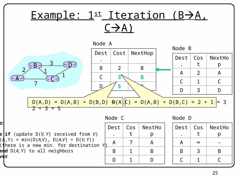
Dest. Cost NextHop
B 2 B
C 3 B
D 5 B
Node A
Example: 1st Iteration (BA, CA)
A C12
7
B D3
1
Dest. Cost NextHop
A 2 A
C 1 C
D 3 D
Node B
Dest. Cost NextHop
A 7 A
B 1 B
D 1 D
Node C
Dest. Cost NextHop
A ∞ -
B 3 B
C 1 C
Node D
D(A,D) = D(A,B) + D(B,D) = 2 + 3 = 5 D(A,C) = D(A,B) + D(B,C) = 2 + 1 = 3
7 loop: …13 else if (update D(V, Y) received from V) 14 D(A,Y) = min(D(A,V), D(A,V) + D(V, Y))15 if (there is a new min. for destination Y)16 send D(A, Y) to all neighbors 17 forever
26
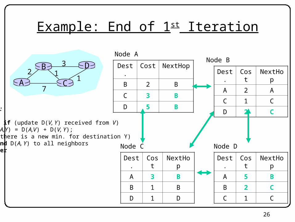
Example: End of 1st Iteration
A C12
7
B D3
1
Dest. Cost NextHop
B 2 B
C 3 B
D 5 B
Node A
Dest. Cost NextHop
A 2 A
C 1 C
D 2 C
Node B
Dest. Cost NextHop
A 3 B
B 1 B
D 1 D
Node C
Dest. Cost NextHop
A 5 B
B 2 C
C 1 C
Node D
7 loop: …13 else if (update D(V, Y) received from V) 14 D(A,Y) = D(A,V) + D(V, Y);15 if (there is a new min. for destination Y)16 send D(A, Y) to all neighbors 17 forever
27
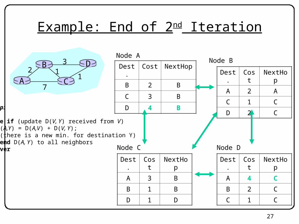
Example: End of 2nd Iteration
A C12
7
B D3
1
Dest. Cost NextHop
B 2 B
C 3 B
D 4 B
Node A
Dest. Cost NextHop
A 2 A
C 1 C
D 2 C
Node B
Dest. Cost NextHop
A 3 B
B 1 B
D 1 D
Node C
Dest. Cost NextHop
A 4 C
B 2 C
C 1 C
Node D
7 loop: …13 else if (update D(V, Y) received from V) 14 D(A,Y) = D(A,V) + D(V, Y);15 if (there is a new min. for destination Y)16 send D(A, Y) to all neighbors 17 forever

28
Example: End of 3rd Iteration
A C12
7
B D3
1
Dest. Cost NextHop
B 2 B
C 3 B
D 4 B
Node A
Dest. Cost NextHop
A 2 A
C 1 C
D 2 C
Node B
Dest. Cost NextHop
A 3 B
B 1 B
D 1 D
Node C
Dest. Cost NextHop
A 4 C
B 2 C
C 1 C
Node D
Nothing changes algorithm terminates
7 loop: …13 else if (update D(V, Y) received from V) 14 D(A,Y) = D(A,V) + D(V, Y);15 if (there is a new min. for destination Y)16 send D(A, Y) to all neighbors 17 forever
29
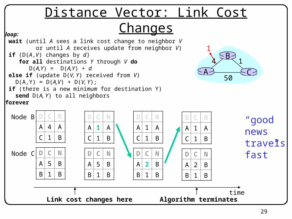
Distance Vector: Link Cost Changes
A C
14
50
B1
“goodnews travelsfast”
D C N
A 4 A
C 1 B
Node B
D C N
A 5 B
B 1 B
Node C
D C N
A 1 A
C 1 B
D C N
A 5 B
B 1 B
D C N
A 1 A
C 1 B
D C N
A 2 B
B 1 B
D C N
A 1 A
C 1 B
D C N
A 2 B
B 1 B
Link cost changes heretime
7 loop:8 wait (until A sees a link cost change to neighbor V 9 or until A receives update from neighbor V) 10 if (D(A,V) changes by d) 11 for all destinations Y through V do 12 D(A,Y) = D(A,Y) + d 13 else if (update D(V, Y) received from V) 14 D(A,Y) = D(A,V) + D(V, Y);15 if (there is a new minimum for destination Y)16 send D(A, Y) to all neighbors 17 forever
Algorithm terminates
30
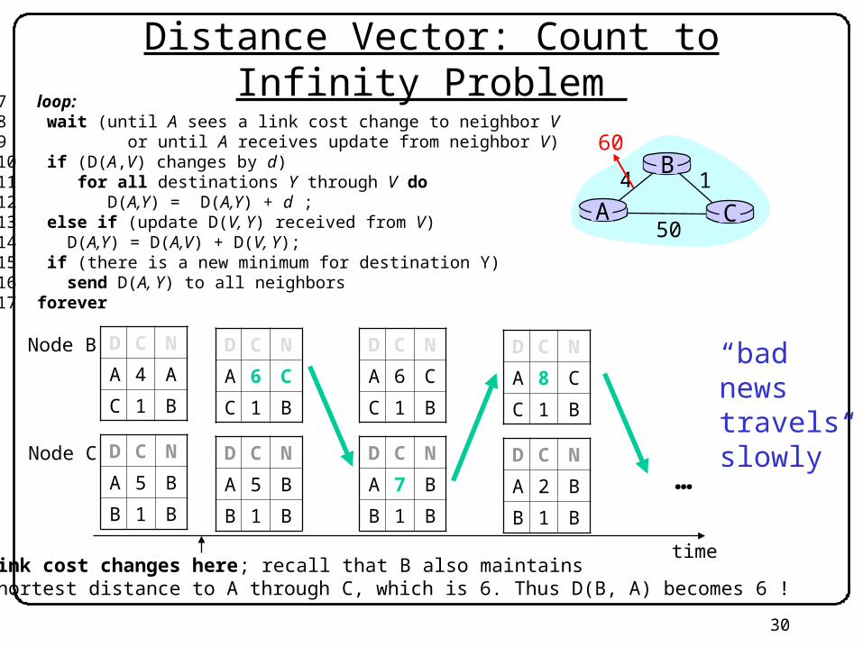
Distance Vector: Count to Infinity Problem
A C
14
50
B60
“badnews travelsslowly”
D C N
A 4 A
C 1 B
Node B
D C N
A 5 B
B 1 B
Node C
D C N
A 6 C
C 1 B
D C N
A 5 B
B 1 B
D C N
A 6 C
C 1 B
D C N
A 7 B
B 1 B
D C N
A 8 C
C 1 B
D C N
A 2 B
B 1 B
Link cost changes here; recall that B also maintains shortest distance to A through C, which is 6. Thus D(B, A) becomes 6 !
time
7 loop:8 wait (until A sees a link cost change to neighbor V 9 or until A receives update from neighbor V) 10 if (D(A,V) changes by d) 11 for all destinations Y through V do 12 D(A,Y) = D(A,Y) + d ;13 else if (update D(V, Y) received from V) 14 D(A,Y) = D(A,V) + D(V, Y);15 if (there is a new minimum for destination Y)16 send D(A, Y) to all neighbors 17 forever
…

31
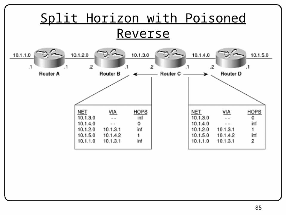
Distance Vector: Poisoned Reverse
A C
14
50
B60 If C routes through B to get to A:
- C tells B its (C’s) distance to A is infinite (so B won’t route to A via C)
D C N
A 4 A
C 1 B
Node B
D C N
A 5 B
B 1 B
Node C
D C N
A 60 A
C 1 B
D C N
A 5 B
B 1 B
D C N
A 50 A
B 1 B
Link cost changes here; B updates D(B, A) = 60 as
C has advertised D(C, A) = ∞
time
D C N
A 60 A
C 1 B
D C N
A 50 A
B 1 B
D C N
A 51 C
C 1 B
D C N
A 50 A
B 1 B
D C N
A 51 C
C 1 B
Algorithm terminates
32
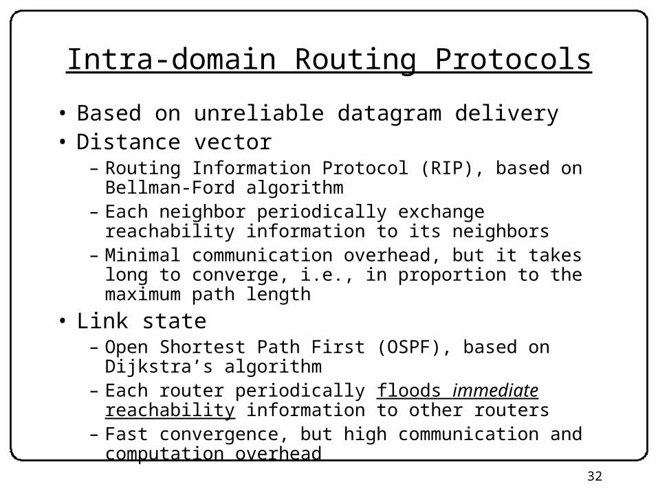
Intra-domain Routing Protocols
• Based on unreliable datagram delivery• Distance vector
– Routing Information Protocol (RIP), based on Bellman-Ford algorithm
– Each neighbor periodically exchange reachability information to its neighbors
– Minimal communication overhead, but it takes long to converge, i.e., in proportion to the maximum path length
• Link state– Open Shortest Path First (OSPF), based on Dijkstra’s
algorithm– Each router periodically floods immediate reachability
information to other routers– Fast convergence, but high communication and computation
overhead
33
Routing Protocol Review
Part 2: Inter-domain routing
34
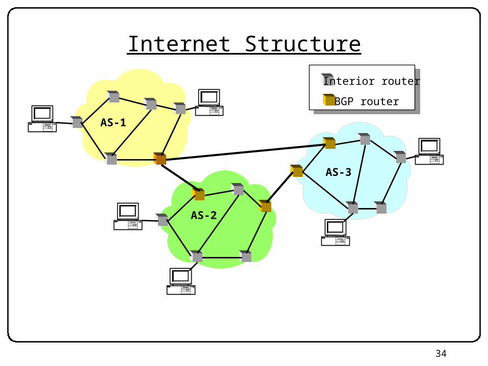
Internet Structure
AS-1
AS-2
AS-3
Interior router
BGP router

35
Intra-Domain
AS-1
AS-2
AS-3
Interior router
BGP router
Intra-domain routing protocol aka Interior Gateway Protocol (IGP), e.g. OSPF, RIP
36
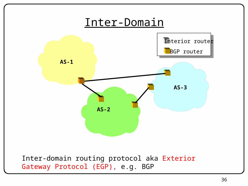
Inter-Domain
AS-2
Interior router
BGP router
Inter-domain routing protocol aka Exterior Gateway Protocol (EGP), e.g. BGP
AS-1
AS-3
37
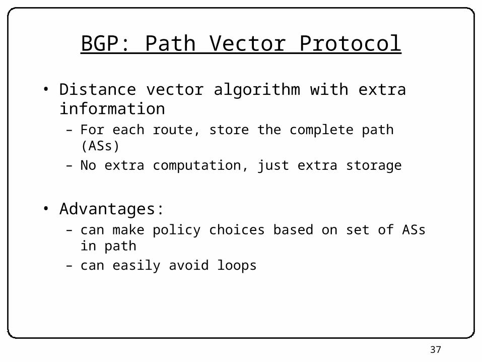
BGP: Path Vector Protocol
• Distance vector algorithm with extra information– For each route, store the complete path (ASs)– No extra computation, just extra storage
• Advantages:– can make policy choices based on set of ASs in path– can easily avoid loops

38
BGP Operations (Simplified)
Establish session on TCP port 179
Exchange all active routes
Exchange incremental updates
AS1
AS2
While connection is ALIVE exchangeroute UPDATE messages
BGP session
39
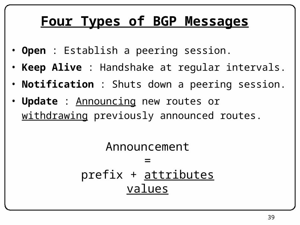
Four Types of BGP Messages
• Open : Establish a peering session.
• Keep Alive : Handshake at regular intervals.
• Notification : Shuts down a peering session.
• Update : Announcing new routes or withdrawing previously
announced routes.
Announcement=
prefix + attributes values

40
Attributes are Used to Select Best Routes
192.0.2.0/24pick me!
192.0.2.0/24pick me!
192.0.2.0/24pick me!
192.0.2.0/24pick me!
Given multipleroutes to the sameprefix, a BGP speakermust pick at mostone best route
(Note: it could reject them all!)

41
Example: Multiple AS Paths
AS701
AS73
AS7018
AS1239
AS9 128.2/16
128.2/169 701
128.2/169 7018 1239

42
Routing Protocol Review
Part 3: Multicast Routing
43
Example Uses of Multicast
• Internet TV radio• Stock price update• Video conference• Spam?!

44
This approach does not scale…
BackboneISP
BroadcastCenter

45
Use routers in distribution tree
BackboneISP
BroadcastCenter
Copy data at routersAt most one copy of a data packet per link
LANs implement link layer multicast by broadcasting
Routers compute trees and forward packets along them
46
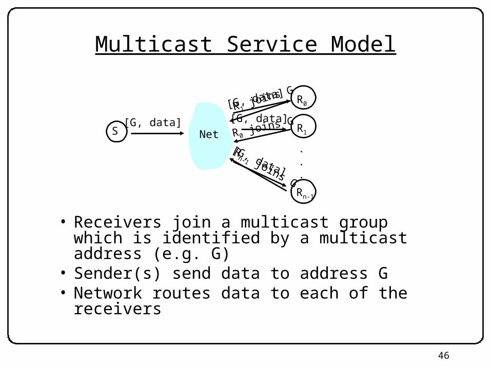
Multicast Service Model
• Receivers join a multicast group which is identified by a multicast address (e.g. G)
• Sender(s) send data to address G• Network routes data to each of the receivers
R0 joins G
R1 joins G
Rn-1 joins G
S
R0
R1
.
.
.
[G, data]
[G, data]
[G, data]
[G, data]
Rn-1
Net
47
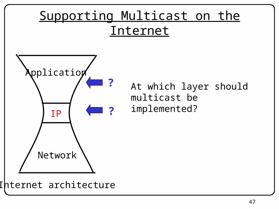
Supporting Multicast on the Internet
IP
Application
Internet architecture
Network
?
?
At which layer should multicast be implemented?
48
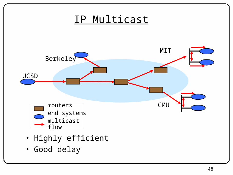
IP Multicast
CMU
BerkeleyMIT
UCSD
routersend systemsmulticast flow
• Highly efficient• Good delay
49
Failure of IP Multicast
• Not widely deployed even after 15 years!– Use carefully – e.g., on LAN or campus, rarely over WAN
• Various failings– Scalability of routing protocols– Hard to manage– Hard to implement TCP equivalent– Hard to get applications to use IP Multicast without existing
wide deployment– Hard to get router vendors to support functionality and hard
to get ISPs to configure routers to enable
50
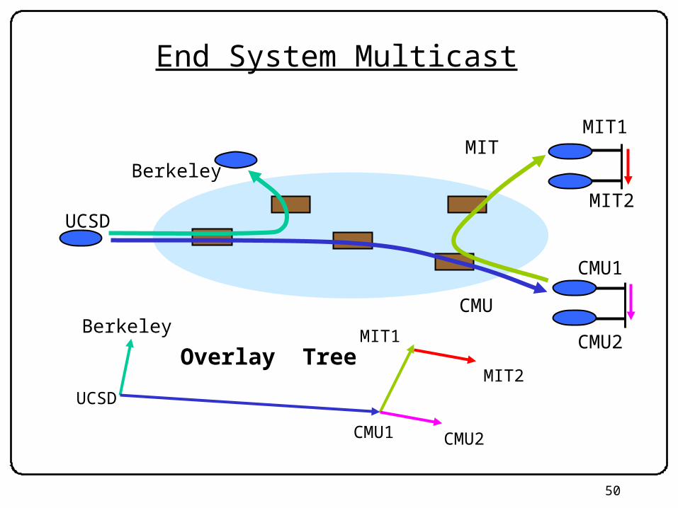
End System Multicast
MIT1
MIT2
CMU1
CMU2
UCSD
MIT1
MIT2
CMU2
Overlay Tree
Berkeley
CMU1
CMU
BerkeleyMIT
UCSD

51
• Quick deployment• All multicast state in end systems• Computation at forwarding points simplifies support
for higher level functionality
Potential Benefits Over IP Multicast
MIT1
MIT2
CMU1
CMU2
CMU
BerkeleyMIT
UCSD
52
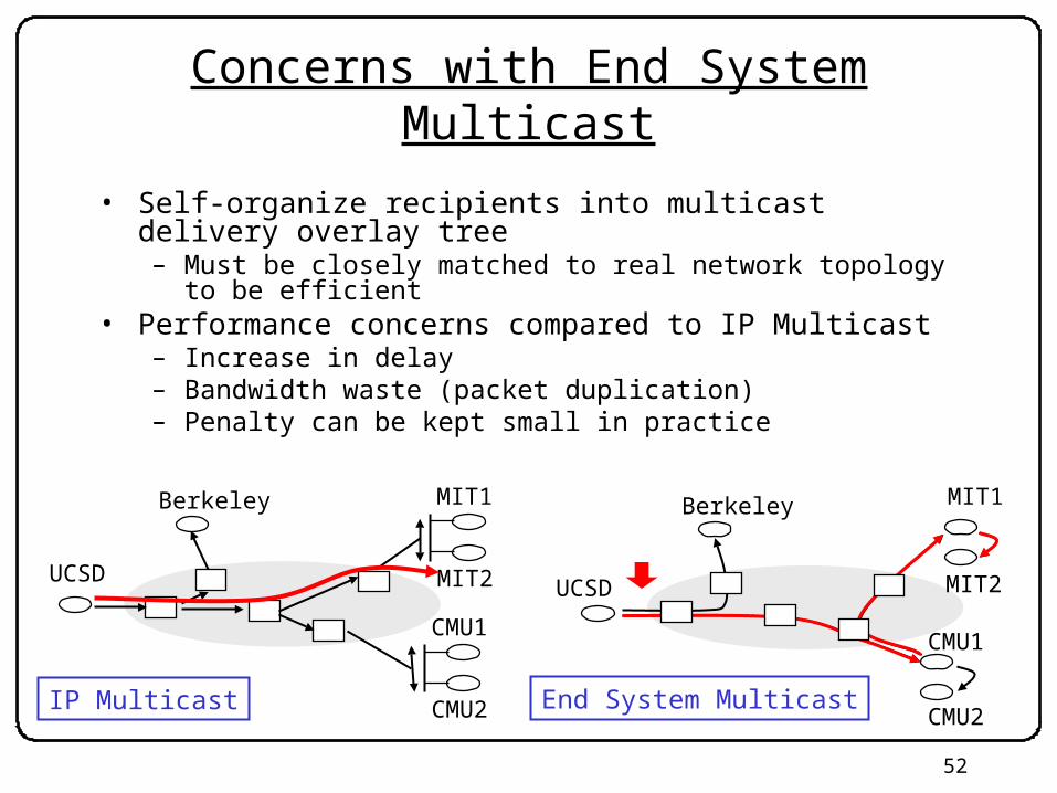
Concerns with End System Multicast
• Self-organize recipients into multicast delivery overlay tree– Must be closely matched to real network topology to be efficient
• Performance concerns compared to IP Multicast– Increase in delay– Bandwidth waste (packet duplication)– Penalty can be kept small in practice
MIT2
Berkeley MIT1
UCSD
CMU2
CMU1
IP Multicast
MIT2
Berkeley MIT1
CMU1
CMU2
UCSD
End System Multicast

53
Multicast: Take-away
• Multicast provides support for efficient data delivery to multiple recipients
• Difficult to deploy IP multicast• End system-based techniques can provide similar
efficiency and it is easier to deploy

54
55
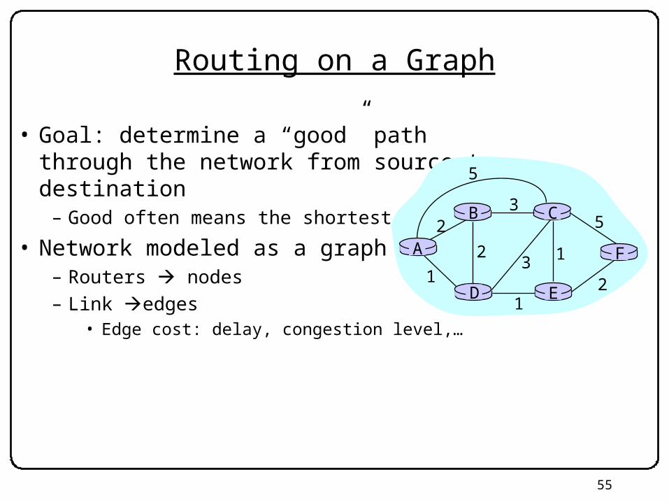
Routing on a Graph
• Goal: determine a “good” path through the network from source to destination
– Good often means the shortest path
• Network modeled as a graph– Routers nodes– Link edges
• Edge cost: delay, congestion level,…
A
ED
CB
F
2
2
13
1
1
2
53
5
56
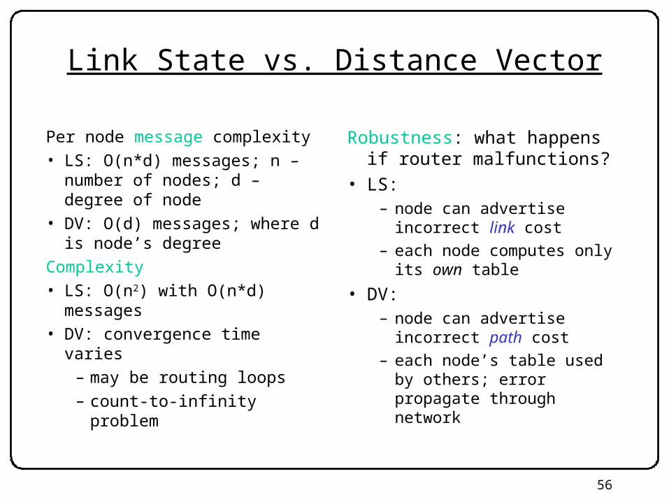
Link State vs. Distance Vector
Per node message complexity• LS: O(n*d) messages; n –
number of nodes; d – degree of node
• DV: O(d) messages; where d is node’s degree
Complexity• LS: O(n2) with O(n*d)
messages• DV: convergence time varies
– may be routing loops– count-to-infinity problem
Robustness: what happens if router malfunctions?
• LS: – node can advertise incorrect
link cost
– each node computes only its own table
• DV:– node can advertise incorrect
path cost
– each node’s table used by others; error propagate through network
57
Routing between ISPs
• Routing protocol (BGP) contains reachability information (no metrics)– Not about optimizing anything– All about policy (business and politics)
• Why?– Metrics optimize for a particular criteria– AT&T’s idea of a good route is not the same as UUnet’s– Scale
• What a BGP speaker announces or not announces to a peer determines what routes may get used by whom

58
Nontransit vs. Transit ASes
ISP 1ISP 2
Nontransit ASmight be a corporateor campus network.
NET ATraffic NEVER flows from ISP 1through NET A to ISP 2(At least not intentionally!)
IP traffic
Internet Serviceproviders (often)have transit networks
59
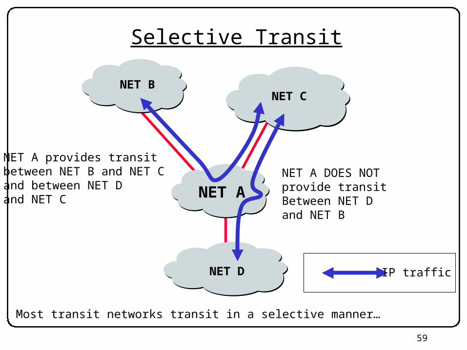
Selective Transit
NET BNET C
NET A provides transitbetween NET B and NET Cand between NET D and NET C NET A
NET D
NET A DOES NOTprovide transitBetween NET D and NET B
Most transit networks transit in a selective manner…
IP traffic
60
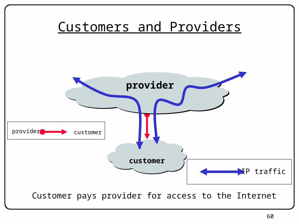
Customers and Providers
Customer pays provider for access to the Internet
provider
customerIP traffic
provider customer

61
Customers Don’t Always Need BGP
provider
customer
Default route 0.0.0.0/0pointing to provider.
Configured route 192.0.2.0/24pointing to customer
192.0.2.0/24
Static routing is the most common way of connecting anautonomous routing domain to the Internet. This helps explain why BGP is a mystery to many …
62
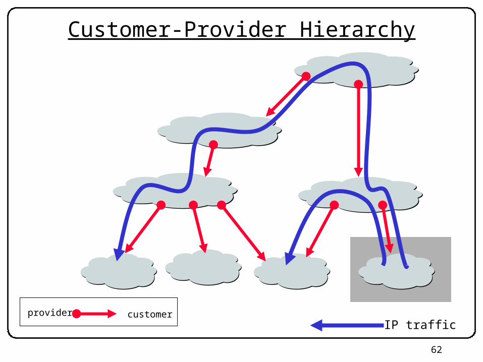
Customer-Provider Hierarchy
IP trafficprovider customer

63
The Peering Relationship
peer peer
customerprovider
Peers provide transit between their respective customers
Peers do not provide transit between peers
Peers (often) do not exchange $$$trafficallowed
traffic NOTallowed
64
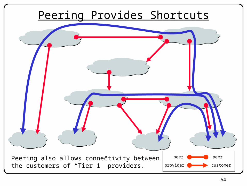
Peering Provides Shortcuts
Peering also allows connectivity betweenthe customers of “Tier 1” providers.
peer peer
customerprovider

65
Implementing Customer/Provider and Peer/Peer relationships
• What you announce determines what route can be used by whom
• Enforce transit relationships – Outbound route filtering
• Enforce order of route preference– provider < peer < customer

66
Import Routes
Frompeer
Frompeer
Fromprovider
Fromprovider
From customer
From customer
provider route customer routepeer route ISP route

67
Export Routes
Topeer
Topeer
Tocustomer
Tocustomer
Toprovider
From provider
provider route customer routepeer route ISP route
filtersblock
68
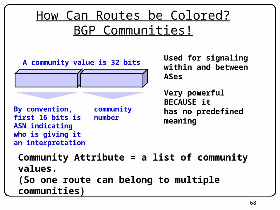
How Can Routes be Colored?BGP Communities!
A community value is 32 bits
By convention, first 16 bits is ASN indicating who is giving itan interpretation
communitynumber
Very powerful BECAUSE it has no predefinedmeaning
Community Attribute = a list of community values.(So one route can belong to multiple communities)
Used for signalingwithin and betweenASes
69
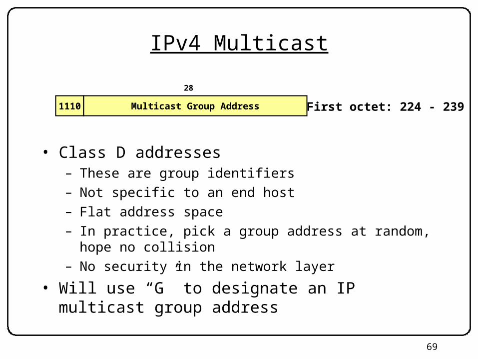
IPv4 Multicast
• Class D addresses– These are group identifiers– Not specific to an end host– Flat address space– In practice, pick a group address at random, hope no
collision– No security in the network layer
• Will use “G” to designate an IP multicast group address
1110 Multicast Group Address
28
First octet: 224 - 239
70
Multicast Implementation Issues
• How is join implemented?• How is send implemented?• How much information about trees is kept and who
keeps it?
71
IP Multicast Routing
• Intra-domain– Distance-vector multicast– Link-state multicast
• Inter-domain– Protocol Independent Multicast, Sparse Mode
• Key idea: Core-Based Tree
72
Distance Vector Multicast Routing Protocol (DVRMP)
• An elegant extension to DV routing• Use shortest path DV routes to determine if link is on
the source-rooted spanning tree• Three steps in developing DVRMP
– Reverse Path Flooding– Reverse Path Broadcasting– Truncated Reverse Path Broadcasting
73
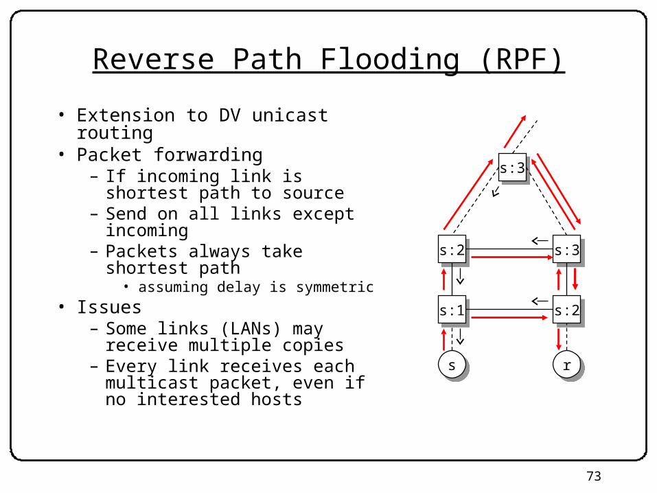
Reverse Path Flooding (RPF)
• Extension to DV unicast routing• Packet forwarding
– If incoming link is shortest path to source
– Send on all links except incoming– Packets always take shortest path
• assuming delay is symmetric• Issues
– Some links (LANs) may receive multiple copies
– Every link receives each multicast packet, even if no interested hosts
s:2s:2
ss
s:1s:1
s:3s:3
s:2s:2
s:3s:3
rr

74
Example
• Flooding can cause a given packet to be sent multiple times over the same link
• Solution: Called “Reverse Path Broadcasting”
xx yy
zz
SS
a
b
duplicate packet

75
Reverse Path Broadcasting (RPB)
• Chose parent of each link along reverse shortest path to source
• Only parent forward to a link (child link)
• Use DV routing update to identify parent
xx yy
zz
SS
a
b
5 6
child link of xfor S
forward onlyto child link
76
Don’t Really Want to Flood!
• This is still a broadcast algorithm – the traffic goes everywhere
• Need to “Prune” the tree when there are subtrees with no group members
• Solution: Truncated Reverse Path Broadcasting
77
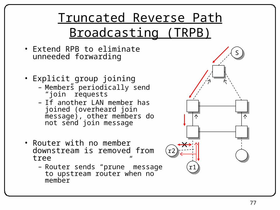
Truncated Reverse Path Broadcasting (TRPB)
• Extend RPB to eliminate unneeded forwarding
• Explicit group joining– Members periodically send “join”
requests– If another LAN member has joined
(overheard join message), other members do not send join message
• Router with no member downstream is removed from tree
– Router sends “prune” message to upstream router when no member
r1r1
r2r2
SS
78
Distance Vector Multicast Scaling
• State requirements: – O(Sources Groups) active state
79
Core Based Trees (CBT)
• The key idea in Inter-domain PIM-SM protocol• Pick a “rendezvous point” for the group called the core
– Build a tree towards the core
– Union of the unicast paths from members to the core
– Shared tree
• To send, unicast packet to core and bounce it back to multicast group
• Reduce routing table state from O(S x G) to O(G)
80
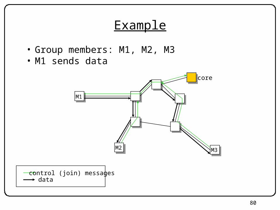
Example
• Group members: M1, M2, M3• M1 sends data
core
M1
M2 M3
control (join) messagesdata

81
Disadvantages
• Sub-optimal delay• Single point of failure
– Core goes out and everything lost until error recovery elects a new core
• Small, local groups with non-local core– Need good core selection– Optimal choice (computing topological center) is NP hard
82
Why Need the Concept of AS or Domain?
• Routing algorithms are not efficient enough to deal with the size of the entire Internet
• Different organizations may want different internal routing policies
• Allow organizations to hide their internal network configurations from outside
• Allow organizations to choose how to route across multiple organizations (BGP)
• Basically, easier to compute routes, more flexibility, more autonomy/independence

83
RIP
From the book: Routing TCP/IP Volume I (CCIE Professional Development)
84
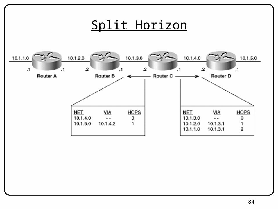
Split Horizon
85
Split Horizon with Poisoned Reverse

86
Counting to Infinity

87
Purpose of E-BGP
R border router
internal router
E-BGPR2
R1
R3
A
AS1
AS2
you can reachnet A via me
table at R1:dest next hopA R2
Share connectivity information across ASes

88
Part II: I-BGP, Carrying Info within an AS
R border router
internal router
R1
AS1
R4
R5
B
AS3
E-BGP
R2R3
A
AS2 announce B
I-BGP
E-BGP
89
I-BGP
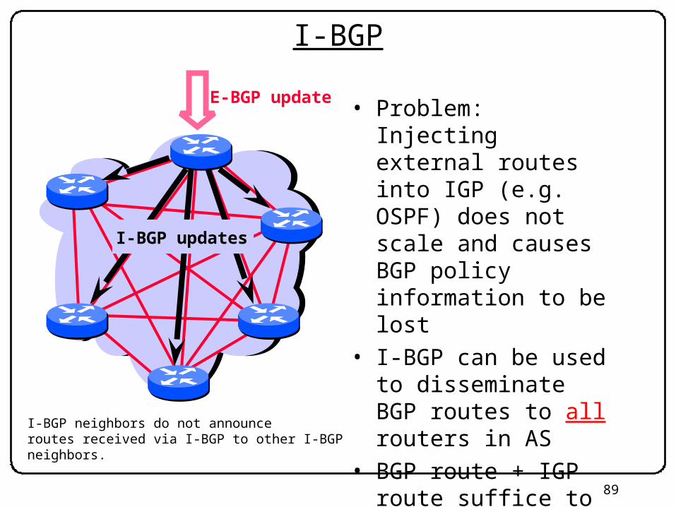
I-BGP neighbors do not announce routes received via I-BGP to other I-BGPneighbors.
E-BGP update
I-BGP updates
• Problem: Injecting external routes into IGP (e.g. OSPF) does not scale and causes BGP policy information to be lost
• I-BGP can be used to disseminate BGP routes to all routers in AS
• BGP route + IGP route suffice to create forwarding table
90
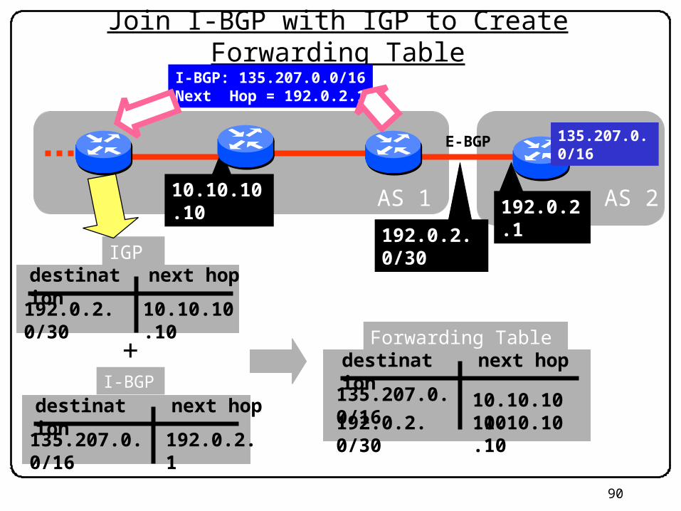
Join I-BGP with IGP to Create Forwarding Table
AS 1 AS 2192.0.2.1
135.207.0.0/16
10.10.10.10
I-BGP: 135.207.0.0/16Next Hop = 192.0.2.1
192.0.2.0/30
Forwarding Table
135.207.0.0/16
destination next hop
10.10.10.10192.0.2.0/30 10.10.10.10
I-BGP
192.0.2.1135.207.0.0/16
destination next hop
+
IGP
10.10.10.10192.0.2.0/30
destination next hop
E-BGP
91
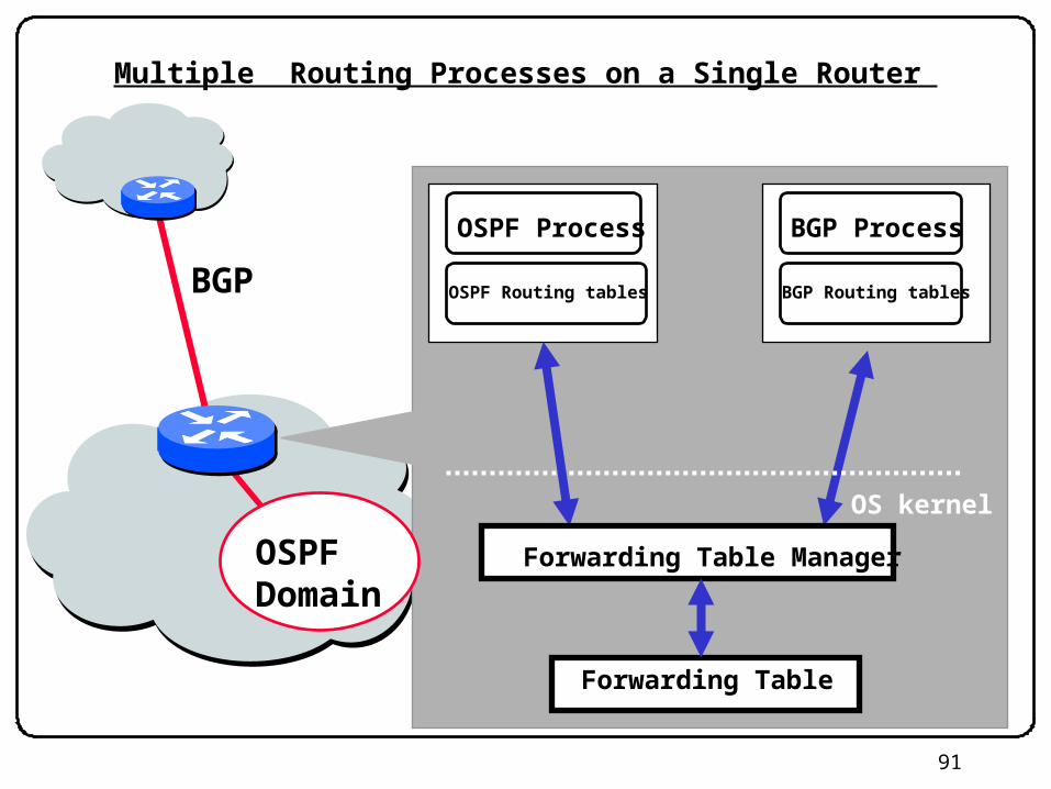
Multiple Routing Processes on a Single Router
Forwarding Table
OSPFDomain
BGP
OS kernel
OSPF Process
OSPF Routing tables
BGP Process
BGP Routing tables
Forwarding Table Manager
92
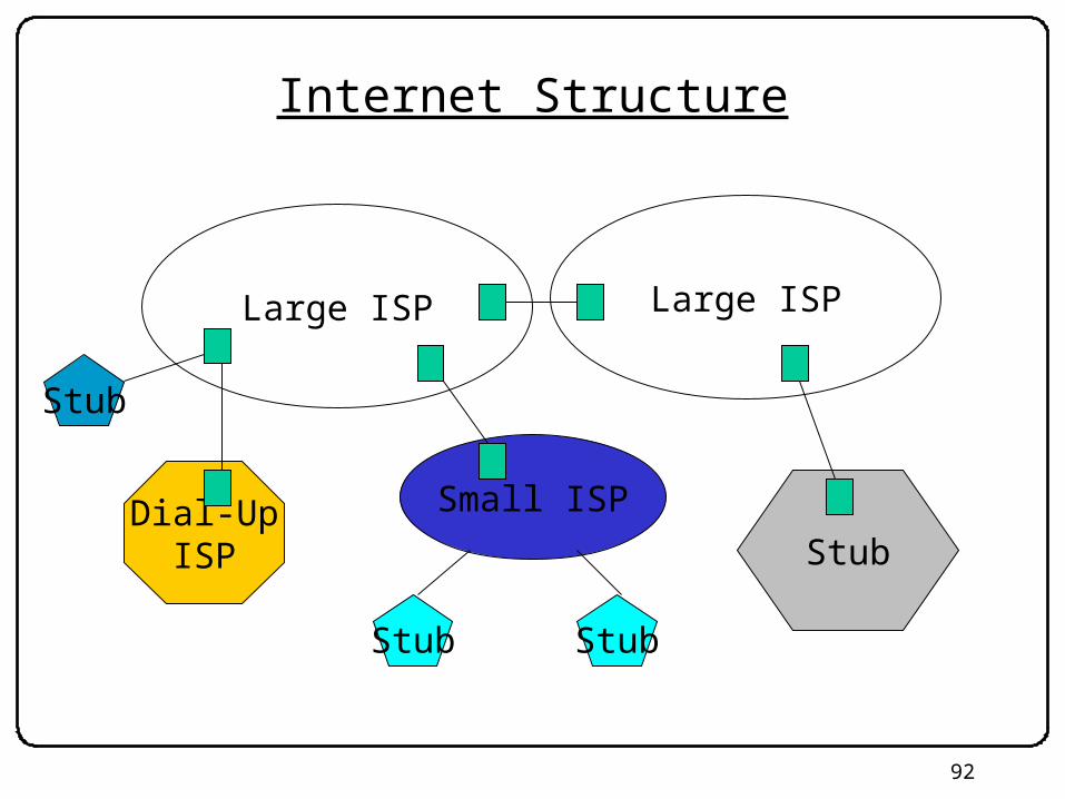
Internet Structure
Large ISP Large ISP
Dial-UpISP Stub
Small ISP
Stub Stub
Stub

93
Inter-Domain Routing
• Global connectivity is at stake• Inevitably leads to one single protocol that everyone
must speak– Unlike many choices in intra-domain routing
• What are the requirements?• Scalability• Flexibility in choosing routes• If you were to choose, link state based or distance
vector based?
• BGP is sort of a hybrid: Path vector protocol
94
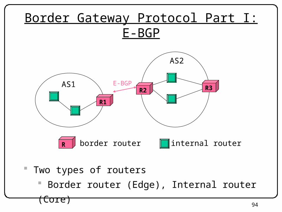
Border Gateway Protocol Part I: E-BGP
R border router internal router
E-BGPR2
R1
R3AS1
AS2
Two types of routers
Border router (Edge), Internal router (Core)

95
Example AS Graph
The subgraph showing all ASes that have more than 100 neighbors in fullgraph of 11,158 nodes. July 6, 2001. Point of view: AT&T route-server
Does not reflect true topology
96
BGP Issues
• BGP designed for policy not performance
• Susceptible to router misconfiguration– Blackholes: announce a route you cannot reach
• Incompatible policies – Solutions to limit the set of allowable policies

97
More Issues
• Scaling the I-BGP mesh– Confederations– Route Reflectors
• BGP Table Growth– 140K prefixes and growing – Address aggregation (CIDR)– Address allocation
• AS number allocation and use• Dynamics of BGP
– Inherent vs. accidental oscillation – Rate limiting and route flap dampening– Lots and lots of redundant info– Slow convergence time

98
Autonomous Systems (AS)
• Internet is not a single network!
• The Internet is a collection of networks, each controlled by different administrations
• An autonomous system (AS) is a network under a single administrative control
99
AS Numbers (ASNs)
ASNs are 16 bit values.64512 through 65535 are “private”
• Genuity: 1 • AT&T: 7018, 6341, 5074, … • UUNET: 701, 702, 284, 12199, …• Sprint: 1239, 1240, 6211, 6242, …• …
Currently over 11,000 in use.

100
Implications
• ASs want to choose own local routing algorithm– AS takes care of getting packets to/from their own hosts– Intradomain routing: RIP, OSPF, etc
• ASs want to choose own non-local routing policy– Interdomain routing must accommodate this– BGP is the current interdomain routing protocol– BGP: Border Gateway Protocol

101
Shorter Doesn’t Always Mean Shorter
AS 4
AS 3
AS 2
AS 1
Path 4 1 is “better” than path 3 2 1

102
Multicast Routing Approaches
• Kinds of Trees– Source Specific Trees
• Most suitable for single sender
• E.g. internet radio
– Shared Tree• Multiple senders in a group
• E.g. Teleconference
• Group
103
Source Specific Trees
6
7
8
5
4
31
2
12
10
13
11
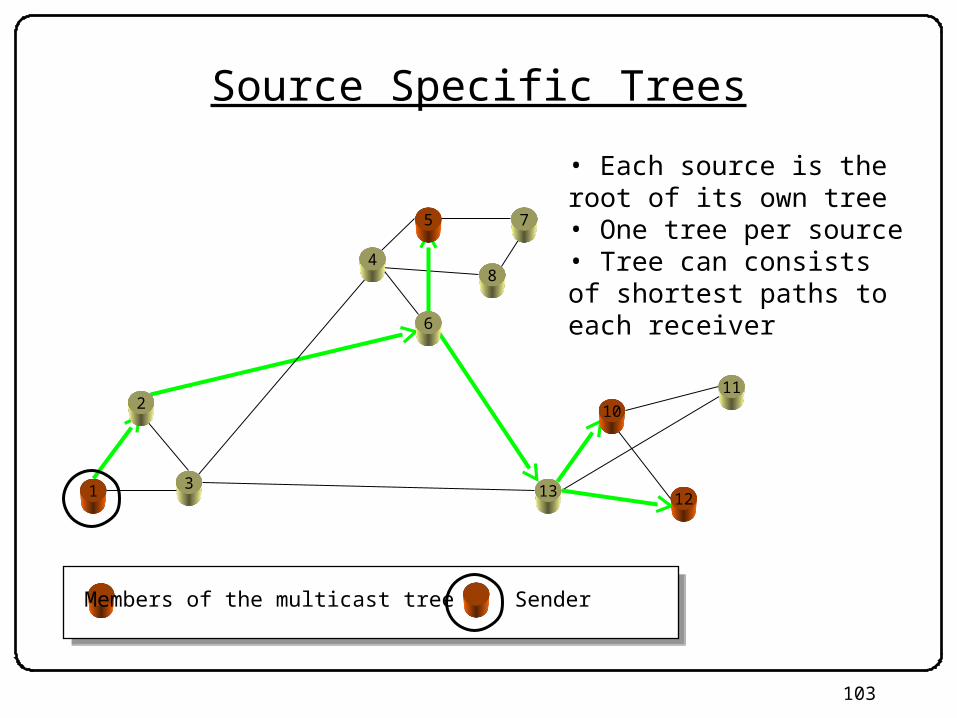
• Each source is the root of its own tree• One tree per source• Tree can consists of shortest paths to each receiver
Members of the multicast tree Sender

104
Source Specific Trees
6
7
8
5
4
31
2
12
10
13
11
Very good performance butexpensive to construct/maintain;routers need to manage a tree per source
• Each source is the root of its own tree• One tree per source• Tree can consists of shortest paths to each receiver
105
Shared Tree
6
7
8
5
4
31
2
12
10
13
11
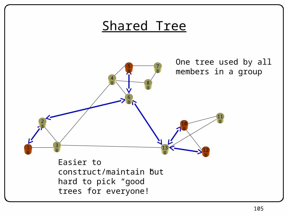
One tree used by all members in a group
Easier to construct/maintain but hard to pick “good” trees for everyone!
106
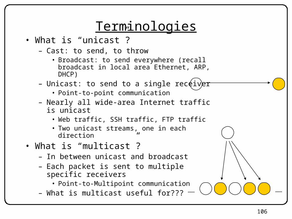
Terminologies• What is “unicast”?
– Cast: to send, to throw• Broadcast: to send everywhere (recall broadcast
in local area Ethernet, ARP, DHCP)
– Unicast: to send to a single receiver• Point-to-point communication
– Nearly all wide-area Internet traffic is unicast• Web traffic, SSH traffic, FTP traffic• Two unicast streams, one in each direction
• What is “multicast”?– In between unicast and broadcast– Each packet is sent to multiple specific
receivers• Point-to-Multipoint communication
– What is multicast useful for???…… ……

107
How to Send to Multiple Receivers?
• What are the simplest ways?• Ex1: Send a copy of the packet to one receiver at a
time until all receivers have it– i.e. use unicast to implement multicast
• Ex2: Flood a packet throughout the network and have non-receivers discard the packet– i.e. use broadcast to implement multicast
• Advantages? Disadvantages?
• In general: We want a distribution tree– Many ways to do it– Big research topic for a decade

108
Example: Internet Radio
• www.digitallyimported.com– Sends out 128Kb/s MP3 music streams– Peak usage ~9000 simultaneous streams– Consumes ~1.1Gb/s
• bandwidth costs are large fraction of their expenditures
– A fat and shallow tree– Does not scale!


