
Risk management optimization for sovereign debt restructuring
Andrea Consiglio ∗
Stavros A. Zenios †
August 2014.
Working Paper 14-10The Wharton Financial Institutions Center
The Wharton School, University of Pennsylvania, PA
Abstract
Debt restructuring is gaining acceptance as a policy tool for resolving sovereign debtcrises. In this paper we propose a scenario analysis for debt sustainability and integrateit with scenario optimization for the risk management of re-profiling sovereign debt. Thescenario dynamics of debt are used to define a risk metric –conditional Debt-at-Risk– for thetail of debt-to-GDP ratios, and a multi-period stochastic programming model optimizes theexpected cost of financing a debt structure, subject to limits on the risk. The model handlesimportant technical aspects of debt restructuring: it collects all debt issues in a commonframework, and can include embedded options and contingent claims, multiple currenciesand step-up or linked contractual features. Alternative debt profiles are then analyzed fortheir cost vs risk tradeoffs. With a suitable re-calculation of the efficient frontier, debtsustainability of a given debt profile can then be ascertained. The model is applied to twostylized examples drawn from an IMF publication and from the Cyprus debt crisis.
Keywords: sovereign debt; debt restructuring; scenario analysis; portfolio optimization; stochas-tic programming.
∗University of Palermo, Palermo, IT. [email protected]†University of Cyprus, Nicosia, CY and The Wharton Financial Institutions Center, University of Pennsylva-
nia, USA. [email protected]
1

1 The sovereign debt restructuring challenge
On May 20, 2013, the International Monetary Fund issued a public notice that its ExecutiveBoard had discussed developments in sovereign debt restructuring and the implications for theFund’s legal and policy framework, IMF (2013). There had not been any discussions at the IMFabout sovereign debt restructuring since 2005, and it had been more than ten years since AnneKrueger’s signature proposal on a sovereign debt restructuring mechanism was rejected understrong opposition from creditor countries, Krueger (2002). If approved, the new Fund policywill introduce the possibility of maturity extensions for countries whose debt is not consideredsustainable. Debt rescheduling and, perhaps, restructuring will become an official policy tool.
The renewed interest was prompted by the realization, in the aftermath of the Greek crisis,that “debt restructurings have often been too little and too late [...] thus failing to re-establishdebt sustainability and market access in a durable way”. Sovereign debt defaults are prevalent asshown in two databases compiled recently, Beers and Nadeau (2014); Trebesch (2011). Figure 1summarizes statistics on debt default worldwide from 1975 to 2013. Greece holds the recordwith the largest sovereign debt restructuring in history (in 2012) and other recent restructuringsinclude Belize (in 2007 and 2013), Jamaica (in 2010 and 2013), and St. Kitts and Nevis (2012).The litigation against Argentina in New York courts by holdouts from the restructuring of 2005is expected to have significant ramifications for future sovereign debt restructurings; the latestruling against Argentina came in June and pushed the country back into (technical) default.
The eurozone crisis highlighted that sovereign defaults are not the privilege of emergingmarkets, developing economies or ill-run autocracies. It happens to the best economies asSturzenegger and Zettelmeyer (2006) show studying ten years of crises; the record is held bya eurozone country after all. The literature documents historical track records of advancedeconomies where debt restructuring, financial repression, and high inflation were an integralpart of the resolution of debt crisis. The depositor bail-in and capital controls imposed onCyprus in March 2013, see Zenios (2014), and the Greek debt restructuring, are recent episodesof financial repression in advanced economies.
Given the complexity of inter-related risk factors in the debt of sovereigns, there is a need foradvances in the risk management of public debt. In general, it has been assumed that marketswill impose discipline on sovereigns and keep their debt in sustainable territory. However,for many reasons, this does not happen and when a sovereign debtor enters a crisis zone thecreditors bolt for the exit. No one is left to roll over debt and the official sector is left to handlethe crisis. In the case of Greece, the Troika of IMF-EC-ECB demanded involvement of privatecreditors before the official sector would bail out the country. The Greek PSI saw 106 billioneuro transferred from private creditors to Greece and an international assistance package of164 billion under strict austerity measures that drove the Greek economy into recession for fiveconsecutive years with unemployment rising to 27%.
While Greece has been an extreme example of debt crisis -and of mismanagement of doingtoo little and too late, see, e.g., Zettelmeyer et al. (2013)- it is not a unique case of advancedeconomies facing debt crises. Figure 2 illustrates the increase of sovereign debt of selectedeurozone countries after the international crisis of 2008. The current average debt of eurozonecountries exceeds the debt-to-GDP ratio of 60% prescribed in the stability and growth pact ofthe European Union. At 96% it exceeds the 90% threshold of Reinhart and Rogoff (2010), andwhile this rigid threshold was recently discredited by Herndon et al. (2014), the conclusion thatexcessive debt is a drag on growth is supported by other studies, Cecchetti et al. (2011).
Debt is fragile and when a sovereign loses market access —it has a “Minsky moment” to quotethe popular term coined in McCulley (2013)— the results are not easily reversed. Many factorscome into play: higher borrowing rates for the distressed sovereign, snowball effect of debtservicing on the country’s GDP and its ability to re-pay, the bank-sovereign “diabolical loop”of Brunnermeier et al. (2011) discussed in Mody and Sandri (2011) for eurozone, capital flight
2

Figure 1: Sovereign debt default worldwide. (Data from Beers and Nadeau (2014).)
De Grauwe (2012). All these factors create negative feedback loops and reversing the viciouscircle requires drastic action. This is where debt restructuring comes into play. Recognizingthat several eurozone countries are in the crisis zone, credible proposals have emerged for debtrestructuring, see, e.g., Gianviti et al. (2010); Paris and Wyplosz (2014). It is in this settingthat the IMF discussions take place.
In this paper we argue for a risk management approach to the re-profiling of public debt. Weuse the broader term re-profiling to include both rescheduling and restructuring of debt, wherebycreditors may suffer losses in present or nominal value. Risk management is not restricted tothe static analysis of debt sustainability. Instead, it requires policymakers to postulate plausiblescenarios and develop risk metrics that ensure high probability of debt sustainability. We adoptfor sovereign debt crisis management the same quantitative approach used for risk managementof portfolios or the asset/liability management of financial institutions, see, e.g. Mulvey andZiemba (1998); Zenios and Ziemba (2007).
Of course, risk management has also failed us in many instances and we do not imply thatwhat we suggest is a foolproof method. Nevertheless, it is a much richer framework. Ourapproach is in line with recent trends in public debt management that are moving beyondsimulation modelling to integrate simulations with optimization, and tradeoff expected costwith Cost-at-Risk, Balibek and Koksalan (2010); Bolder and Rubin (2011); Consiglio and Staino(2012).
We start with a discussion of debt restructuring issues in section 2 and then discuss scenarioanalysis for debt re-profiling in Section 3. We develop a scenario optimization model for min-imizing Conditional Debt-at-Risk and explain how various issues arising in debt restructuringcan be addressed either by the model or by suitable modifications and post-optimality analysis.The use of the model is illustrated on two stylized examples obtained from an IMF publicationand for restructuring the Cyprus debt in section 4, and conclusions are summarized in section 5.
2 Sovereign debt re-profiling: why and how
When a sovereign faces a debt crisis it may be advisable to re-profile its debt in a manner thatpreserves value for both debtor and creditors. There is certainly no benefit to the creditors if
3
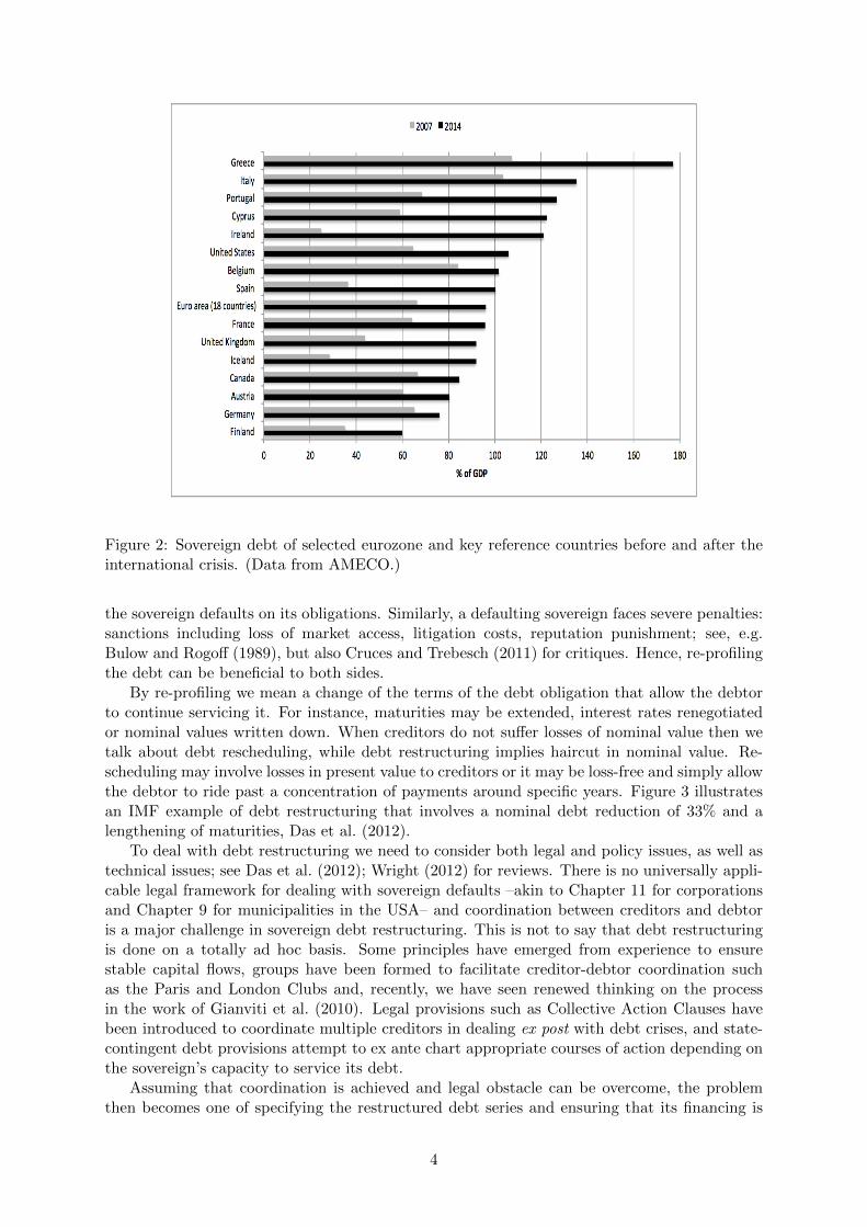
Figure 2: Sovereign debt of selected eurozone and key reference countries before and after theinternational crisis. (Data from AMECO.)
the sovereign defaults on its obligations. Similarly, a defaulting sovereign faces severe penalties:sanctions including loss of market access, litigation costs, reputation punishment; see, e.g.Bulow and Rogoff (1989), but also Cruces and Trebesch (2011) for critiques. Hence, re-profilingthe debt can be beneficial to both sides.
By re-profiling we mean a change of the terms of the debt obligation that allow the debtorto continue servicing it. For instance, maturities may be extended, interest rates renegotiatedor nominal values written down. When creditors do not suffer losses of nominal value then wetalk about debt rescheduling, while debt restructuring implies haircut in nominal value. Re-scheduling may involve losses in present value to creditors or it may be loss-free and simply allowthe debtor to ride past a concentration of payments around specific years. Figure 3 illustratesan IMF example of debt restructuring that involves a nominal debt reduction of 33% and alengthening of maturities, Das et al. (2012).
To deal with debt restructuring we need to consider both legal and policy issues, as well astechnical issues; see Das et al. (2012); Wright (2012) for reviews. There is no universally appli-cable legal framework for dealing with sovereign defaults –akin to Chapter 11 for corporationsand Chapter 9 for municipalities in the USA– and coordination between creditors and debtoris a major challenge in sovereign debt restructuring. This is not to say that debt restructuringis done on a totally ad hoc basis. Some principles have emerged from experience to ensurestable capital flows, groups have been formed to facilitate creditor-debtor coordination suchas the Paris and London Clubs and, recently, we have seen renewed thinking on the processin the work of Gianviti et al. (2010). Legal provisions such as Collective Action Clauses havebeen introduced to coordinate multiple creditors in dealing ex post with debt crises, and state-contingent debt provisions attempt to ex ante chart appropriate courses of action depending onthe sovereign’s capacity to service its debt.
Assuming that coordination is achieved and legal obstacle can be overcome, the problemthen becomes one of specifying the restructured debt series and ensuring that its financing is
4

Figure 3: Debt with and without restructuring; from the IMF report of Das et al. (2012).
sustainable. Das et al. (2012) provide the key parameter specifications of the problem:
1. Face and market value of bonds or loans
2. Interest rate and coupon (fixed vs flexible, step-up or linked features)
3. Amortization schedule (bullet vs amortization, existence of a sinking fund)
4. Currency of denomination of the instruments (local vs foreign currency)
5. Enhancements, including embedded options or collateral
6. Legal clauses (CACs, non-default clauses, exit consents).
2.1 The need for a model
The issues relating to the implementation of debt restructuring are discussed in depth by Wright(2012) who makes several suggestions on the need for reform. Perhaps his most importantsuggestion, and the one most relevant to our work, is the development of “criteria for an“optimal” debt restructuring process. “Optimal” is put within quotes by the author, recognizingthat in such a complex setting there is no unique optimality criterion. His work addressesinstitutional, legal and instrumental issues of restructuring, for which one can not expect amathematical optimum. However, the suggestions point to the need for a model to coordinatethe process. Such a model would capture the tasks of the “international debt referee”, canaddress “the greatest problem which is restricted to restructuring a single debt”, and accountfor the central role of “state contingent debt”. It would provide the decision support tool forthe sovereign debt restructuring framework discussed at the IMF in Krueger (2002), and for theeurozone in Gianviti et al. (2010).
The scenario optimization model we develop next handles the technical aspects of debt re-structuring. First, it collects all debt issues in a common framework and under a set of scenariosthat capture consistently the relevant risk factors. Second, it develops optimal financing strate-gies for alternative debt profiles and trades off their cost and associated risks using an optimalitycriterion that captures debt sustainability. Third, embedded options and contingent claims can
5

Tt210
NTNtN2N1N0
Figure 4: A scenario tree.
readily be modelled conditioned on the scenarios. Fourth, the currency of denomination can bemodelled via exchange rate scenarios. Fifth, the model is multi-period so we can model sinkingfunds and step-up or linked contractual features. We do not include all these features in thecurrent model. The basic model developed in this paper deals with the first two items, butextensions are discussed.
3 Scenario analysis for optimal debt restructuring
3.1 The choice of a model
The model is a multi-period stochastic program. Decisions are made here-and-now based onall available information, and anticipating future uncertain information. As new information isobtained and uncertainty resolved we have the recourse decisions that are conditioned on therealized scenario and on prior decisions. Stochastic programming models have a rich history infinancial management over the last twenty years; see Zenios (2007); Zenios and Ziemba (2007)and the extensive bibliography therein. Recently such models received attention for public debtmanagement in the works of Balibek and Koksalan (2010); Consiglio and Staino (2012). Ourmodel extends Consiglio and Staino (2012) to debt re-profiling. A multi-period model capturessome key features of the debt re-profiling problem: it allows us to integrate multiple debt issueswith different maturities that may extend well into the future, and can account for clustering ofmaturities around specific dates with the associated roll-over risk. Clustering of debt maturitiesaround specific dates, usually following government elections, is prevalent in sovereign debtmanagement, as the political process borrows during a government’s term and pushes paymentto the next government. Note, for instance, in Figure 8 of Cyprus debt, the large payments duein 2014, just after the presidential elections of 2013.
3.2 The scenario setting
We consider now the setting where the key economic and financial variables evolve accordingto some stochastic processes. The processes may be correlated. In scenario modeling we adopta discrete set of time-stages when decisions are taken, denoted by T = {0, 1, 2...t...T}. t = 0
6

denotes here-and-now where all information is known, T is the risk horizon and t is the timeindex, see, e.g. (Zenios, 2007, chap. 5) . At each time instance t, data evolve on a scenario tree,such as the one illustrated in Figure 4, whereby problem data can take values from a set indexedby the set of nodes Nt. Each node n ∈ Nt represents possible future states of the economy attime t. Not all nodes at t can be reached from every node at t− 1 and we define paths from theroot node 0 to some final node in the set NT to denote the unique way of reaching a particularnode. Each of these paths is a scenario. Our example has 12 scenarios, two possible statesat t = 0, three possible states at t = 1 and six at t. We denote by n ∈ Nt nodes in the setsNt for each t = 0, 1, 2, . . . T . We denote by P(n) the set of nodes on the unique path from theroot node to n ∈ Nt, and by p(n) the unique predecessor node for n, with p(0) being empty. Atany given node n all information contained in its predecessor p(n) and the path P(n) is known.
With this notation we now define state-dependent fiscal variables for each node n ∈ Nt:
GDP, denoted by Gn in nominal value with growth rate gn.
Debt, denoted by Dn in nominal value and dn as a ratio to GDP.
Interest on debt, denoted by rn. For countries under an assistance program the interest maybe fixed at r0 for all time periods until the end of the program or even beyond.
Government net budget, denoted by NBn, and the following relation applies:
NBn = GTn −GEn. (1)
GT denotes government revenues, typically taxes, and GE denotes government expen-ditures excluding debt servicing costs. For states of the economy with NBn > 0 thegovernment is running a structural surplus that can be used to pay down debt or accu-mulate reserves. Conversely, NBn < 0 denotes structural deficit that increases debt.
Stock flow adjustment of debt, denoted by SFn in nominal value and sf n as a ratio toGDP.
We assume that all debt is in domestic currency. Technical modifications of everything thatfollows are possible to account for foreign debt and exchange rate risks; see, e.g., Sturzeneg-ger and Zettelmeyer (2006) eqns. (A.10)-(A.18) for the inter-temporal dynamics on a singledeterministic scenario, or Topaloglou et al. (2002) eqns. (13)-(14) for multi-currency scenariomodeling including exchange rate hedging. We develop our model in a single currency for easeof notation and avoid one more risk factor in the stylized examples consider later.
3.3 Scenario arithmetic for fiscal dynamics
The general debt stock recursive equation is as follows, see, e.g., Ley (2010):
Dt = (1 + rt)Dt−1 −NB t + SF t. (2)
Ley uses seignorage as SF t. We use stock flow adjustment to represent adjustments to the debtprofile via restructuring or rescheduling. If a sovereign can collect seignorage, then SF needs tobe split in a seignorage term and a debt restructuring term, and seignorage modeled separately.In the scenario setting the debt dynamics are conditioned on the nodes:
Dn = (1 + rn)Dp(n) −NBn + SFn. (3)
This equation is defined for every node on the tree. It can be solved recursively for each pathleading from the root to each terminal node n ∈ NT . While there is only one solution to
7

equation (2) for the deterministic case, we have as many solutions to equation (3) as there arepaths to terminal states in the scenario setting.
We express the debt dynamics as a ratio to GDP to account for “snowball effect”, i.e.,the improvement/deterioration of the debt situation of a country by growth/contraction of theeconomy. GDP growth is a significant risk factor in debt crises and the debt-to-GDP ratio stockdynamics are expressed conditioned on the state of the economy denoted by n, derived directlyfrom the scenario-independent debt dynamics.
Dn
Gn= (1 + rn)
Dp(n)
Gp(n)
Gp(n)
Gn− NBp(n)
Gn+
SFn
Gn. (4)
GDP growth is given by
gn =Gn −Gp(n)
Gn, (5)
and we express the debt dynamics in proportional growth instead of nominal value by:
dn =1 + rn
1 + gndp(n) − nbn + sf n. (6)
We can use this equation to derive conditions for debt sustainability to answer questionssuch as “How can a government maintain a constant debt-to-GDP ratio?”, or, “How to reducedebt-to-GDP ratio to a level that is sustainable?”. For instance, debt is stable if dn = dp(n) forthe paths to all terminal nodes, and the primary surplus to ensure this is given by:
nbn
=rn − gn1 + gn
dp(n) + sf n. (7)
When primary balance satisfies nbn > nbn
debt will be reduced in direct proportion tothe primary balance. Assuming no debt restructuring, i.e., sf n = 0 and balanced budget, i.e.,nbn = 0, the debt is stable if growth equals effective interest rate on debt rn = gn. Growth issuppressed during crises, requiring strictly positive primary balance to maintain constant debt.Fiscal consolidation, in turn, exerts downward pressure on GDP exacerbating the crisis. Hence,there is a limit to how much can be achieved with surplus-generating austerity once a countryis in crisis. That is when debt restructuring enters as a policy option. The question is thenposed on which combination of primary surplus and debt restructuring will reduce debt by aproportion β to bring it to sustainable level.
To reduce debt by dn = βdp(n) we have the following debt stock equation:
nbn =
[1 + rn
1 + gn− β
]dp(n) + sf n. (8)
This equation provides the relationship between the two key policy variables: primary surplusachieved with austerity measures and debt restructuring. However, the use of scenarios high-lights the difficulty in making deterministic statements for the policy variable. The equationprovides different values for each scenario and we need to adopt some risk metric, such as usingthe worst case value, or the expected value or some acceptable quintile.
3.4 Scenario optimization
3.4.1 Model equations
We consider now the funding of government debt with a sequence of decisions x = {xt}t=0,1,...,T .These decisions could include borrowing from the international market, loans of different ma-turities and contractual obligations from international organizations as part of an assistanceprogram, or bi-lateral agreements with friendly governments. x0 is the here-and-now decision
8

and xt are the recourse decisions that are conditioned on the state of the economy. xt is a set ofpossible decision vectors {xnt }n∈Nt . Without ambiguity we drop the time index from xn sinceeach node n takes values from a time-indexed set Nt. If we assume there are J available optionsfor funding debt, then the decision vector is given by
xn = (xn1, xn2 . . . xnJ).
We now express the debt dynamics on the scenario tree in terms of funding decisions. Foreach t = 0, 1, . . . , T − 1, and each n ∈ Nt we have:
On =∑
m∈P(n)
J∑j=1
xmjCF j(n,m), (9)
where CF j(n,m) denotes cash flows at node n for any debt issued at some node m ∈ P(n).1 O0
is the nominal debt due here-and-now. This equation accounts for the total debt to be coveredat each node n due to decisions made at previous time periods.
The debt stock equation takes into account obligations created by previous funding decisionsand existing debt, and requires that this stock is financed from new funding decisions:
J∑j=1
xnj = Dn +On. (10)
At the end of the horizon T and for each n ∈ NT we have the cost of our decisions:
Cn = Dn +On +∑
m∈P(n)
J∑j=1
xmjP j(n,m). (11)
P j(n,m) is the state-dependent value of debt and it can be given in nominal value, ifwe follow the accounting standards for sovereign debt reporting, or by market value if weare interested in fair valuation for the sovereign’s creditors. The use of market values requirescontingent re-pricing of debt at the different states, see Mulvey and Zenios (1994). The problemof choice between book and market valuation is prevalent in the sovereign debt managementliterature, so much so that there are two approaches of computing sovereign debt haircuts; Daset al. (2012). Using market value is more appropriate for debt buyback situations, while bookvalue is more appropriate for contractual restructuring.
3.4.2 Objective function
We develop the objective function on the debt-to-GDP ratio cn = Cn/Gn which is the keyindicator for debt sustainability; (Sturzenegger and Zettelmeyer, 2006, p. 308-313). Debt-to-GDP is a random variable whose discrete distribution depends on debt financing decisions, onthe schedule of existing debt, on any debt restructuring, and the economic and financial ran-dom variables. The decision maker wants to shape the distribution of this random variableto match some views. For instance, they may want to tradeoff expected value against volatil-ity. Or, more appropriately, consider a target Value-at-Risk that should not be exceeded ora target on the coherent risk measure of conditional Value-at-Risk (CVaR), of Artzner et al.(1999). Alternatively, the public debt management office may have a multitude of objectives
1The calculations of CF are tedious. They take into account coupon and principal payments, perhaps ad-justable rates, contingency provisions and so on. However, all these are exogenous to the debt funding decision.Once a scenario tree is built and a path P(n) specified CF is obtained using standard cash-flow calculators;see (Consiglio and Staino, 2012, eqn. 6) for cash-flow calculations of government bonds and Topaloglou et al.(2002) for bonds in multiple currencies.
9

and wish to trade-off expected cost, duration of debt, volatility of cost or VaR and so on. Thepublic debt management office of the Turkish Ministry of Finance adopts a multi-objective opti-mization framework, Balibek and Koksalan (2010), while Consiglio and Staino (2012) optimizeconditional Cost-at-Risk for the Italian treasury.
Debt sustainability analysis establishes a threshold debt-to-GDP ratio below which thesovereign can service its debt without resorting to additional borrowing. In general 120%is considered the threshold for advanced economies, and this was used for the Greek debtrestructuring. For Cyprus the threshold was estimated at 100%, and to avoid exceeding thisvalue with a bail-out of banks by the state, the depositors were bailed-in instead. These targetsare based on a unique projection of debt-to-GDP which, in our scenario setting, would be themean value. To assess the risk of deviation from a sustainable debt-to-GDP threshold we needa risk measure. We define the stress debt for each terminal state of the economy as the non-negative difference of the state-dependent debt-to-GDP ratio from its expected value. Stressdebt is a signal of problems that debt-to-GDP ratio deviates from a sustainable mean value,and we now formulate its conditional Value-at-Risk, which we call conditional Debt-at-Risk. Let
sdn = cn − E[c], (12)
where E[C] is the expected value of the terminal final debt-to-GDP ratio, i.e.,
E[c] =∑n∈NT
πncn, (13)
where πn are the probabilities of the terminal states. For uniform distributions of child nodesat each non-terminal node, the probabilities are given by 1
|NT | for symmetric trees. For non-symmetric trees, such as the one of Figure 4, terminal probabilities are easily computed as thejoint probability of all nodes on the path P(n). The conditional Debt-at-Risk is the expectedexcess debt over its Value-at-Risk of debt at a given confidence level α and, following Rockafellarand Uryasev (2000), this is obtained as CDaR from the following set of equations:
CDaR = ζ +1
1− α∑n∈NT
πnyn+, (14)
yn+ ≥ sdn − ζ, (15)
yn+ ≥ 0, (16)
where yn+ is a dummy variable denoting the non-negative values of debt in excess of ζ, and ζ isthe Value-at-Risk of the debt.
3.4.3 Model
We have expressed debt dynamics and conditional Debt-at-Risk in terms of exogenous GDPdynamics and debt restructuring decisions, and endogenous debt financing. The following op-timization model minimizes the expected cost of debt with limits on the risk metric CDaR:
10

Minimizexn, n∈N
E[c] (17)
s.t. (18)
On =∑
m∈P(n)
J∑j=1
xmjCF j(n,m) for all n ∈ Nt, t ∈ T \0, (19)
Dn +On =J∑
j=i
xnj , for all n ∈ N , (20)
Cn = Dn +On +∑
m∈P(n)
J∑j=1
xmj P j(n,m), for all n ∈ NT , (21)
sdn = cn − E[c], for all n ∈ NT , (22)
yn+ ≥ sdn − ζ, for all n ∈ NT , (23)
ζ +1
1− α∑n∈NT
πnyn+ ≤ ρ, (24)
xn, On, cn, yn+ ≥ 0, for all n ∈ N . (25)
Varying the bounds on CDaR we trace an efficient frontier and from that we can evaluatedifferent policies and identify those that are sustainable at the α confidence level.
4 Stylized examples from Cyprus and the IMF
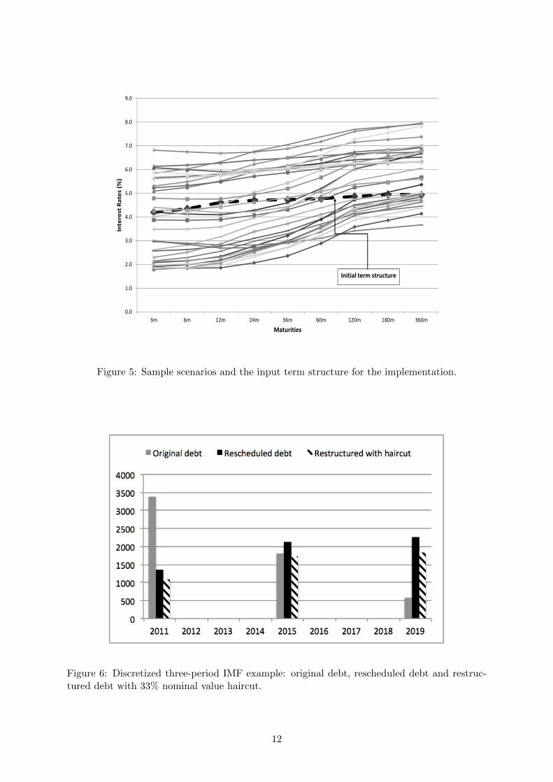
We use two examples drawn from an IMF publication and the debt crisis in Cyprus. Theapplications are stylized and further validation is needed before the results can be used toguide specific policies. However, key features of debt restructuring are captured and allow usto illustrate how risk profiles change with alternative debt restructuring policies and to showhow sustainable policies can be identified. Interest rate scenarios were generated using thesimulator of Bernaschi et al. (2007). The main input data are (i) the current term structure,(ii) the ECB official rate, and (iii) the current inflation rate. Using this information and fittedparameters for the short rate model, we generate a set of scenarios of lengths 12 months. Thenext stage scenarios are simulated by starting from the relevant data of the previous month andthe procedure is repeated for each scenario and for each stage. Figure 5 illustrates the scenariosand the input term structure we use. The confidence level is set to 95%.
4.1 The IMF example
We work with a three-period discretization of the example from Das et al. (2012) shown inFigure 6. In this example we are not given any information on the size of the economy, so insteadof optimizing our risk metric for debt-to-GDP ratios, we work directly with debt (i.e., GDP isset equal to 1). We run the model to optimize the financing of three different debt structuresand compare the efficient frontiers (i) for the original debt, (ii) the rescheduled debt, and (iii)the restructured debt with nominal debt reduction. Figure 7 illustrates the improvements in thetradeoffs. The improvements, in this example, are very large, reflecting the fact that the originaldebt was heavily front loaded and therefore rescheduling was very effective. Further savings ofabout 40% of expected cost are realized by the 33% haircut. However, without information onsize of GDP we can not tell which points on the frontiers correspond to sustainable debt.
11
4.0
5.0
6.0
7.0
8.0
9.0
Inte
rest
Ra
tes (
%)
0.0
1.0
2.0
3.0
3m 6m 12m 24m 36m 60m 120m 180m 360m
Inte
rest
Ra
tes (
%)
Maturities
Initial term structure
Figure 5: Sample scenarios and the input term structure for the implementation.
Figure 6: Discretized three-period IMF example: original debt, rescheduled debt and restruc-tured debt with 33% nominal value haircut.
12

6000#
7000#
8000#
9000#
10000#
11000#
12000#
13000#
14000#
15000#
00# 100# 200# 300# 400# 500# 600# 700# 800# 900#
Expe
cted
(cost(
CDaR(/Condi2onal(Debt/at/Risk(
Oiginal#debt# Rescheduled#debt# Restructured#with#haircut#
Figure 7: Risk profiles for the IMF debt example with rescheduling and restructuring.
4.2 The Cyprus example
The Cyprus debt crisis, while small in absolute numbers –GDP was EUR18 billion at theonset of the crisis corresponding to 0.2% of the eurozone economy– is one of the most complexin the eurozone. Zenios (2013) gives a review of the crisis as it developed until March 2013when a rescue package was agreed with international lenders and explains why Cyprus faces a“perfect crisis”. With the Greek PSI of 2011 the two major banks of Cyprus suffered significantlosses and required about EUR4 bil. to satisfy capital requirements while a subsequent duediligence by PIMCO –taking into account nonperforming loans under deteriorating economicconditions– estimated capital shortfalls of 5.98 bil. and 8.87 bil. under a base and adversescenario, respectively. These estimates were criticized in Zenios (2014) as being excessive by afactor of two, and an investigation by NY Times also questioned the estimates, but neverthelessthese were the numbers used to define bank recapitalization needs 2. They represent 35-55% ofGDP to be added to 2012 public debt of 85.6% GDP. The resulting capital needs could not beresolved with an IMF-ECB-EC bail-out and Cyprus became the first eurozone country wherebank depositors were bailed-in, making international headlines3. The debt profile in Figure 8is based on Cyprus debt position at the end of 2013 and we use GDP projections and fiscalvariables from the debt sustainability analysis of Commission (2013) shown in Figure 9.
We run the optimization model for three test cases of (i) the original debt, (ii) rescheduleddebt, and (iii) restructured debt. The results are summarized in Figure 10. For the originaldebt we also report the range of values for each point on the frontier, based on a sensitivityanalysis of the results by re-running the simulations sixteen times.
What do these results tell us about the sustainability of Cyprus debt? For the country’sGDP of 17 billion in 2013 we could judge that all points on the efficient frontier for the original
2Landon Thomas Jr., July 24, 2014, “A Secret in Cyprus Bank Bailout Stirs Resentment”, NY Times.3Eamonn Fingleton in Forbes, March 17, 2013, “The Botching of the Cyprus Bailout: Worse Than Lehman
Brothers”, Annika Breidthardt and John O’Donnell reporting for Reuters “How Europe stumbled into schemeto punish Cyprus savers”, posted on Monday, Mar 18 17:34 PM GMT
13

Figure 8: Cyprus debt profile (top) and three-period discretization with rescheduling and re-structuring with 20% haircut (bottom).
14

Figure 9: Projections for Cyprus GDP growth and primary surplus. (Data from Commission(2013).)
7"
8"
9"
10"
11"
12"
13"
14"
15"
16"
17"
0" 0.5" 1" 1.5" 2" 2.5" 3" 3.5" 4"
Expe
cted
"Cost"(billion
"euros)"
CDaR"(billion"euro)"
Rescheduled"debt" Restructured"with"haircut" Original"debt"with"error"bounds"
Figure 10: Risk profiles for financing the Cyprus debt with and without restructuring.
15
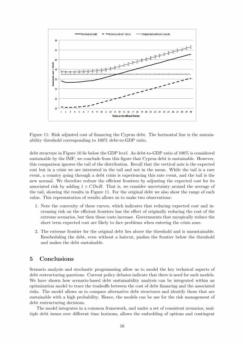
Figure 11: Risk adjusted cost of financing the Cyprus debt. The horizontal line is the sustain-ability threshold corresponding to 100% debt-to-GDP ratio.
debt structure in Figure 10 lie below the GDP level. As debt-to-GDP ratio of 100% is consideredsustainable by the IMF, we conclude from this figure that Cyprus debt is sustainable. However,this comparison ignores the tail of the distribution. Recall that the vertical axis is the expectedcost but in a crisis we are interested in the tail and not in the mean. While the tail is a rareevent, a country going through a debt crisis is experiencing this rate event, and the tail is thenew normal. We therefore redraw the efficient frontiers by adjusting the expected cost for itsassociated risk by adding 1 × CDaR. That is, we consider uncertainty around the average ofthe tail, showing the results in Figure 11. For the original debt we also show the range of eachvalue. This representation of results allows us to make two observations:
1. Note the convexity of these curves, which indicates that reducing expected cost and in-creasing risk on the efficient frontiers has the effect of originally reducing the cost of theextreme scenarios, but then these costs increase. Governments that myopically reduce theshort term expected cost are likely to face problems when entering the crisis zone.
2. The extreme frontier for the original debt lies above the threshold and is unsustainable.Rescheduling the debt, even without a haircut, pushes the frontier below the thresholdand makes the debt sustainable.
5 Conclusions
Scenario analysis and stochastic programming allow us to model the key technical aspects ofdebt restructuring questions. Current policy debates indicate that there is need for such models.We have shown how scenario-based debt sustainability analysis can be integrated within anoptimization model to trace the tradeoffs between the cost of debt financing and the associatedrisks. The model allows us to compare alternative debt structures and identify those that aresustainable with a high probability. Hence, the models can be use for the risk management ofdebt restructuring decisions.
The model integrates in a common framework, and under a set of consistent scenarios, mul-tiple debt issues over different time horizons, allows the embedding of options and contingent
16

claims, can deal with multiple currencies, sinking funds and step-up or linked contractual fea-tures. While not all of these features were modeled and tested, they require only straight-forwardtechnical modifications of the base model.
There are two extensions of the model that deserve further work for the model to be deployedin large-scale real-world applications in crisis countries. First, to simulate the feedback loopbetween austerity and GDP scenarios. At the simplest level this can be done for each stateof the postulated scenarios through fiscal multipliers for the economy of interest. Second, tooptimize the debt restructuring decisions, as oppose to doing risk management optimization ofalternative exogenously given debt structures. This would require a parametrization of the debtstructure and embedding our optimization model into a hierarchical optimization of the debtstructure parameters.
The results with the two stylized examples are very informative, especially for the case ofCyprus where they cast doubt on current beliefs on the sustainability of the country’s debt.Given the insights obtained for the examples, the two extensions discussed above are worthpursuing.
17

References
P. Artzner, F. Delbaen, J. Eber, and D. Heath. Coherent measures of risk. MathematicalFinance, 9(3):203–228, 1999.
E. Balibek and M. Koksalan. A multi-objective multi-period stochastic programming model forpublic debt management. European Journal of Operational Research, 205:205–2017, 2010.
D. T. Beers and J-S. Nadeau. Introducing a New Database of Sovereign Defaults. TechnicalReport No. 101, Bank of Canada, February 2014.
M. Bernaschi, M. Briani, M. Papi, and D. Vergni. Scenario-generation methods for an optimalpublic debt strategy. Quantitative Finance, 7:217–229, 2007.
D.J Bolder and D. Rubin. Optimization in a simulation setting: Use of function approximationin debt strategy analysis. Bank of Canada Working Paper 3, Bank of Canada, 2011.
M.K Brunnermeier, L. Garicano, P.R. Lane, M. Pagano, R. Reis, T. Santos,S. Van Nieuwerburgh, and D. Vayanos. ESBies: a realistic reform of eu-rope’s financial architecture. Technical report, VOXeu.org, 2011. URLhttp://www.voxeu.org/article/esbies-realistic-reform-europes-financial-architecture.
J. Bulow and K.S. Rogoff. Sovereign Debt: Is to Forgive to Forget. American Economic Review,79(1):43–50, July 1989.
S.G. Cecchetti, M.S. Mohanty, and F. Zampolli. The real effects of debt. Technical report,Bank for International Settlement, September 2011.
European Commission. Assessment of the public debt sustainability of Cyprus. Technicalreport, Directorate-General for Economic and Financial Affairs, Brussels, April 2013.
A. Consiglio and A. Staino. A stochastic programming model for the optimal issuance ofgovernment bonds. Annals of Operations Research, 193(1):159–172, 2012.
J.J. Cruces and C. Trebesch. Sovereign Defaults: The Price of Haircuts. Technical report, ifoInstitue, Center for Economic Studies, Munich, October 2011.
S.D. Das, M. Papaioannou, and C. Trebesch. Sovereign Debt Restructurings 1950–2010: Lit-erature Survey, Data, and Stylized Facts. Technical Report Working Paper 12/203, TheInternational Monetary Fund, Washington, DC, 2012.
P. De Grauwe. The Governance of a Fragile Eurozone. Australian Economic Review, 45(3):255–268, 2012.
F. Gianviti, A. O. Krueger, J. Pisani-Ferry, A. Sapir, and J. von Hagen. A European mechanismfor sovereign debt crisis resolution: a proposal. Blueprint Series 10, Bruegel, Brussels, 2010.
T. Herndon, M. Ash, and R. Pollin. Does High Public Debt Consistently Stifle EconomicGrowth? A Critique of Reinhart and Rogoff. Cambridge Journal of Economics, 38(2):257–279, 2014.
IMF. Sovereign debt resturcturing - recent developments and implications for the fund’s legaland institutional framework. Technical report, The International Monetary Fund, April 2013.URL https://www.imf.org/external/np/pp/eng/2013/042613.pdf.
A.O. Krueger. A new approach to sovereign debt restructuring. Technical report, InternationalMonetary Fund, Washington, DC, April 2002.
18
E. Ley. Fiscal (and External) Sustainability. Technical report, The World Bank, Washington,DC, 2010.
P. McCulley. The shadow banking system and Minsky’s journey. In Arthur M Berd, editor,Lessons from the Financial Crisis, pages 49–63. Risk Books, November 2013.
A. Mody and D. Sandri. The eurozone crisis: How banks and sovereigns came to be joined atthe hip. Working paper WP-11-269, The International Monetary Fund, 2011.
J.M. Mulvey and S.A. Zenios. Capturing the correlations of fixed-income instruments. Man-agement Science, 40:1329–1342, 1994.
J.M. Mulvey and W.T. Ziemba, editors. Worldwide asset and liability modeling. CambridgeUniversity Press, 1998.
P. Paris and C. Wyplosz. PADRE-Politically Acceptable Debt Restructuring in the Eurozone.Geneva Reports on the World Economy Special Report 3, International Center for Monterayand Banking Studies, 2014.
C. Reinhart and K.S. Rogoff. Growth in a time of debt. American Economic Review, 100:573–578, January 2010.
R.T. Rockafellar and S. Uryasev. Optimization of conditional Value–at–Risk. Journal of Risk,2(3):21–41, 2000.
F. Sturzenegger and J. Zettelmeyer. Debt defaults and lessons from a decade of crises. MITPress, Cambridge, Mass., 2006.
N. Topaloglou, H. Vladimirou, and S.A. Zenios. CVaR models with selective hedging for inter-national asset allocation. Journal of Banking & Finance, 26(7):1535–1561, 2002.
C. Trebesch. Sovereign debt restructurings 1950-2010: A new database. Unpublished paper,available electronically at https://sites.google.com/site/christophtrebesch/data, University ofMunich, Munich, Gemany, 2011.
M.L.J. Wright. Sovereign debt restructuring: Problems and prospects. Harvard Business LawReview, 2:152–198, 2012.
S.A. Zenios. Practical Financial Optimization: Decision making for financial engineers. Black-well, Malden, MA, 2007.
S.A. Zenios. The Cyprus debt: Perfect crisis and a way forward. Cyprus Economic PolicyReview, 7(1):3–45, 2013.
S.A. Zenios. Fairness and reflexivity in the Cyprus bail-in. Working paper no. 14–04, TheWharton Financial Institutions Center, 2014.
S.A. Zenios and W.T. Ziemba, editors. Handbook of Asset and Liability Management Volume1. Theory and Methodology. Handbooks in Finance. North-Holland, The Netherlands, 2007.
J. Zettelmeyer, C. Trebesch, and M. Gulati. The Greek debt restructuring: an autopsy. Tech-nical Report 9577, Centre for Economic Policy Research, July 2013.
19


