COOPERATIVE GROUNDWATER REPORT 9
ILLINOIS STATE WATER SURVEYILLINOIS STATE GEOLOGICAL SURVEYChampaign, Illinois 61820
RETENTION OF
ZINC, CADMIUM, COPPER, AND LEAD
BY GEOLOGIC MATERIALS
James P. Gibb and Keros Cartwright
Prepared in cooperation withMunicipal Environmental Research LaboratoryU.S. Environmental Protection Agency
STATE OF ILLINOIS DEPARTMENT OF ENERGY AND NATURAL RESOURCES 1982

RETENTION OFZINC, CADMIUM, COPPER, AND LEAD
BY GEOLOGIC MATERIALS
James P. Gibb and Keros Cartwright
STATE WATER SURVEY STATE GEOLOGICAL SURVEY
In cooperation with
Municipal Environmental Research LaboratoryU.S. Environmental Protection Agency
Cincinnati, OH 45268
CHAMPAIGN, ILLINOIS 1982
STATE WATER SURVEYStanley A. Changnon, Jr., Chief
STATE OF ILLINOISHON. JAMES R. THOMPSON, Governor
DEPARTMENT OF ENERGY AND NATURAL RESOURCESMICHAEL B. WITTE, B.A., Director
BOARD OF NATURAL RESOURCES AND CONSERVATION
Michael B. Witte, B.A., Chairman
Walter E. Hanson, M.S., Engineering
Laurence L. Sloss, Ph.D., Geology
H. S. Gutowsky, Ph.D., Chemistry
Lorin I. Nevling, Ph.D., Forestry
Robert L. Metcalf, Ph.D., Biology
Daniel C. Drucker, Ph.D.University of Illinois
John C. Guyon, Ph.D.Southern Illinois University
STATE GEOLOGICAL SURVEYRobert E. Bergstrom, Chief
Printed by authority of the State of Illinois /3000/1982
FOREWORD
This publication summarizes the results of research conducted by theIllinois State Water Survey and State Geological Survey. The research wasfunded in part (Contract No. R-803216) by the Solid and Hazardous WasteResearch Division (SHWRD), Municipal Environmental Research Laboratory,U.S. Environmental Protection Agency, Cincinnati, Ohio. The projectofficer was Mike H. Roulier of SHWRD.
The report has been reviewed by the U.S. Environmental ProtectionAgency and released for publication as a combined report. Approval doesnot signify that the contents necessarily reflect the views and policies ofthe U.S. Environmental Protection Agency, nor does mention of trade namesor commercial products constitute endorsement or recommendation for use byany of the respective agencies.
This report describes a study of the effectiveness of glaciated regionsoils in retaining toxic metals. It also contains an evaluation of severalinvestigative and monitoring techniques for their effectiveness in detect-ing and quantitatively measuring the extent of groundwater contaminationfrom surface waste disposal activities.
James P. GibbHead, Groundwater Section
Illinois State Water Survey
Keros CartwrightHead, Hydrogeology and Geophysics
Illinois State Geological Survey
i i i
ABSTRACT
The vertical and horizontal migration patterns of zinc, cadmium,copper, and lead through the soil and shallow aquifer systems at twosecondary zinc smelters were defined by use of soil coring and monitoringwell techniques. The vertical migration of the same elements at a thirdzinc smelter also was defined. The migration of metals at the threesmelters has been limited by attenuation processes to relatively shallowdepths in the soil profile. Cation exchange and precipitation of insolu-able metal compounds, resulting from pH changes in the infiltratingsolution, were determined to be the principal mechanisms controlling themovement of the metals through the soil. Increased metal contents in theshallow groundwater systems have been confined to the imnediate plants i tes.
Soil coring was found to be an effective investigative tool but wasnot suitable by itself for routine monitoring of waste disposal activities.It should be used to gather preliminary information to aid in determiningthe proper horizontal and vertical locations for monitoring wells. Theanalyses of water samples collected in this project generally did notyield a stable, reproducible pattern of results. This indicates the needto develop techniques to obtain representative water samples. The failureof some well seals in a highly polluted environment also indicates the needfor additional research into monitoring well construction.
iv
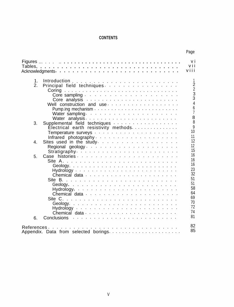
CONTENTS
Figures ... . . . .. . . . . . . . . . . . . . . . . . . . . . . . . . . . . . . . . . v iTables. . . . . . . . . . . . . . . . . . . . . . . . . . . . . . . . . . v i iAcknowledgments. . . . . . . . . . . . . . . . . . . . . . . . . . . . . v i i i
1.2.
3.
4.
5.
3
8
16233251
586469
727481
122
3467
89
10111212151616
51
70
6.
Introduction . . . . . . . . . . . . . . . . . . . . . . . . .Principal field techniques . . . . . . . . . . . . . . . .
Coring . . . . . . . . . . . . . . . . . . . . . . . . . . . . . . . .Core sampling . . . . . . . . . . . . . . . . . . .Core analysis . . . . . . . . . . . . . . . . . . . . . . . .
Well construction and use . . . . . . . . . . . . . . . . . .Pump.ing mechanism . . . . . . . . . . . . . . . . . . . . . . . . .Water sampling. . . . . . . . . . . . . . . . . . . .Water analysis . . . . . . . . . . . . . . . . . . . . . . . .
Supplemental field techniques . . . . . . . . . . . . . . . . .Electrical earth resistivity methods. . . . . . . . . . . . . . .Temperature surveys . . . . . . . . . . . . . . . . . . . .Infrared photography . . . . . . . . . . . . . . . . . . .
Sites used in the study. . . . . . . . . . . . . . . . .Regional geology . . . . . . . . . . . . . . . . . . . .Stratigraphy. . . . . . . . . . . . . . . . . . . . . . . .
Case histories . . . . . . . . . . . . . . . . . . . . . .Site A . . . . . . . . . . . . . . . . . . . . . . . . . . .
Geology. . . . . . . . . . . . . . . . . . . . . . . . . . .Hydrology . . . . . . . . . . . . . . . . . . . . . . . . .Chemical data . . . . . . . . . . . . . . . . . . . . . .
Site B. . . . . . . . . . . . . . . . . . . . . . . . . .Geology.. . . . . . . . . . . . . . . . . . . . . . . .Hydrology.. . . . . . . . . . . . . . . . . . . . . . . .Chemical data . . . . . . . . . . . . . . . . . . . . .
Site C. . . . . . . . . . . . . . . . . . . . . . . . . . .Geology. . . . . . . . . . . . . . . . . . . . . . . . .Hydrology . . . . . . . . . . . . . . . . . . . . . . .Chemical data . . . . . . . . . . . . . . . . . . . . . . .
Conclusions . . . . . . . . . . . . . . . . . . . . . . . . .
References . . . . . . . . . . . . . . . . . . . . . . . . . . . . . . . 82Appendix. Data from selected borings. . . . . . . . . . . . . . . . . . . . . . 85
Page
V
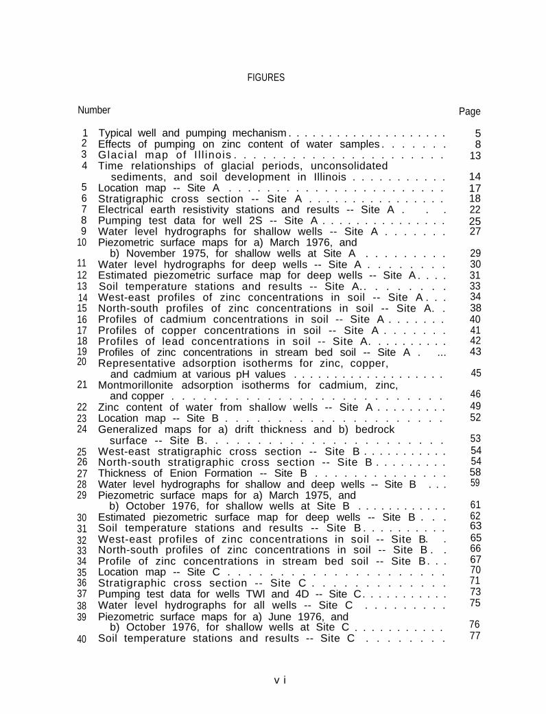
FIGURES
Number Page
1234
56789
10
11121314151617181920
21
222324
2526272829
30313233343536373839
40
58
13
141718222527
29
3130
33
3834
42
49
4041
43
52
45
46
5354
595854
61626365666770717375
7677
Typical well and pumping mechanism . . . . . . . . . . . . . . . . . . . .Effects of pumping on zinc content of water samples . . . . . . .Glacial map of I l l inois . . . . . . . . . . . . . . . . . . . . . .Time relationships of glacial periods, unconsolidated
sediments, and soil development in Illinois . . . . . . . . . . .Location map -- Site A . . . . . . . . . . . . . . . . . . . . . . .Stratigraphic cross section -- Site A . . . . . . . . . . . . . . . .Electrical earth resistivity stations and results -- Site A . . .Pumping test data for well 2S -- Site A . . . . . . . . . . . . . . .Water level hydrographs for shallow wells -- Site A . . . . . . .Piezometric surface maps for a) March 1976, and
b) November 1975, for shallow wells at Site A . . . . . . . . .Water level hydrographs for deep wells -- Site A . . . . . . . .Estimated piezometric surface map for deep wells -- Site A . . . .Soil temperature stations and results -- Site A.. . . . . . . .West-east profiles of zinc concentrations in soil -- Site A . . .North-south profiles of zinc concentrations in soil -- Site A. .Profiles of cadmium concentrations in soil -- Site A . . . . . . .Profiles of copper concentrations in soil -- Site A . . . . . . .Profiles of lead concentrations in soil -- Site A. . . . . . . . . .Profiles of zinc concentrations in stream bed soil -- Site A . ...Representative adsorption isotherms for zinc, copper,
and cadmium at various pH values . . . . . . . . . . . . . . . . . . .Montmorillonite adsorption isotherms for cadmium, zinc,
and copper . . . . . . . . . . . . . . . . . . . . . . . . . .Zinc content of water from shallow wells -- Site A . . . . . . . . .Location map -- Site B . . . . . . . . . . . . . . . . . . . . .Generalized maps for a) drift thickness and b) bedrock
surface -- Site B. . . . . . . . . . . . . . . . . . . . . . .West-east stratigraphic cross section -- Site B . . . . . . . . . . .North-south stratigraphic cross section -- Site B . . . . . . . . .Thickness of Enion Formation -- Site B . . . . . . . . . . . . . .Water level hydrographs for shallow and deep wells -- Site B . . .Piezometric surface maps for a) March 1975, and
b) October 1976, for shallow wells at Site B . . . . . . . . . . . .Estimated piezometric surface map for deep wells -- Site B . . .Soil temperature stations and results -- Site B . . . . . . . . . .West-east profiles of zinc concentrations in soil -- Site B. .North-south profiles of zinc concentrations in soil -- Site B . .Profile of zinc concentrations in stream bed soil -- Site B. . .Location map -- Site C . . . . . . . . . . . . . . . . . . . . .Stratigraphic cross section -- Site C . . . . . . . . . . . . .Pumping test data for wells TWl and 4D -- Site C. . . . . . . . . . .Water level hydrographs for all wells -- Site C . . . . . . . . .Piezometric surface maps for a) June 1976, and
b) October 1976, for shallow wells at Site C . . . . . . . . . . .Soil temperature stations and results -- Site C . . . . . . . .
v i
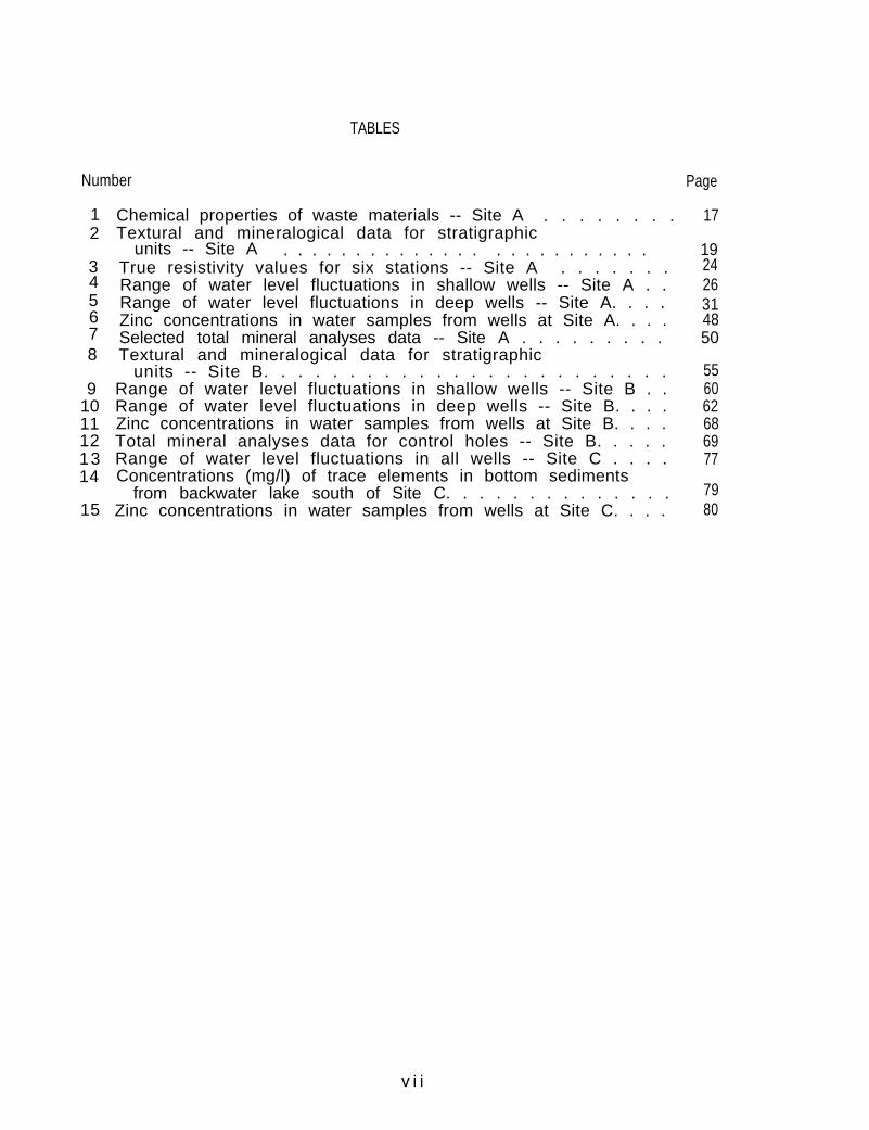
TABLES
Number Page
244
3148
55Range of water level fluctuations in shallow wells -- Site B . .
from backwater lake south of Site C. . . . . . . . . . . . . . 79Zinc concentrations in water samples from wells at Site C. . . . 80
units -- Site B. . . . . . . . . . . . . . . . . . . . . . . .60
Range of water level fluctuations in deep wells -- Site B. . . . 62Zinc concentrations in water samples from wells at Site B. . . . 68Total mineral analyses data for control holes -- Site B. . . . . 69Range of water level fluctuations in all wells -- Site C . . . . 77Concentrations (mg/l) of trace elements in bottom sediments
units -- Site A . . . . . . . . . . . . . . . . . . . . . . . . . True resistivity values for six stations -- Site A . . . . . . .Range of water level fluctuations in shallow wells -- Site A . . 26Range of water level fluctuations in deep wells -- Site A. . . .Zinc concentrations in water samples from wells at Site A. . . .Selected total mineral analyses data -- Site A . . . . . . . . . 50Textural and mineralogical data for stratigraphic
1 Chemical properties of waste materials -- Site A . . . . . . . . 172 Textural and mineralogical data for stratigraphic
193
56
87
91011121314
15
v i i
ACKNOWLEDGMENTS
The authors wish to express their gratitude to the three industriesthat permitted studies to be conducted on their property. In accordancewith the provisions set forth in this study, the names and locations ofthese industries are not specified. Coring and well installations at SitesA and B were done by Layne Western Co., Kirkwood, Missouri; special thanksgo to Marion Scouby, who furnished the drilling crew and technical advice.
Susan S. Wickham and Dave Lindorf of the Illinois State GeologicalSurvey provided geological support. Keith Stoffel and Donald McKaycollected samples during drilling. H. Edward Scoggin operated the drillingrig at Site C. Robert Gilkeson conducted the resistivity and temperaturesurveys and wrote those portions of the report. Dr. W. Arthur Whitesupervised textural analysis of samples, and Dr. Herbert D. Glass performedX-ray analyses of samples.
acquisition, preparation, and storage. Drs. Phillip Hopke and Mary Ulrich
Personnel of the Environmental Research Analytical Laboratory at theUniversity of Illinois conducted all metals analyses under the direction ofArnold Hartley. Paul Schroeter maintained the integrity of sample
conducted X-ray fluorescence analyses. John Healy, Paul Amberg, Brad Hess,Clifford Colgan, and Dr. Donald Bath performed the atomic absorptionmeasurements. Alan Matton, Mary Perez, Susan Gould, and Jean Mitchell didthe electrochemical measurements and the determinations of soil pH andcation exchange capacity.
The project was conducted under the general supervision of John B.Stall, former Head of the Hydrology Section, Illinois State Water Survey.Richard J. Schicht reviewed the manuscript and gave guidance throughout thelatter stages of the project. Steve Wirth and William Bogner tabulated thetables of data; John Brother, Jr., William Motherway, Jr., and June Gibbprepared the illustrations; T. A. Prickett conducted and analyzed thepumping test at Site C; Gail Taylor edited the final report; and PamelaLovett and Lynn Weiss typed the final manuscript.
Special thanks are given to William H. Walker, who conceived andinitiated the project. The patience and understanding of Mike Roulier, theproject officer of the USEPA, helped make possible the transition ofleadership and completion of the project.
v i i i
SECTION 1
INTRODUCTION
Existing air and surface water pollution regulations have forced largevolumes of chemical waste to the land for ultimate disposal. As a result,some aquifers may be in danger of serious water quality degradation ifthese disposal activities are not properly controlled and monitored.
As of 1981, 120 land disposal sites were under permit by the IllinoisEnvironmental Protection Agency to receive special wastes. In addition,more than 2000 active or abandoned landfill sites and private industrialdisposal sites have received large but unknown quantities of all types ofwastes, including some toxic chemicals. Some of these are adjacent to ordirectly underlain by shallow aquifer systems vulnerable to contaminationfrom surface sources.
The amount and area1 extent of hazardous material migration from thesedisposal sites is not known. Some are monitored for possible contaminationor pollution of contiguous aquifers, but only a few appear to be effective-ly instrumented. Traditionally, monitoring wells are installed and watersamples are collected and analyzed periodically. However, these wellsgenerally cannot monitor very large vertical segments of an aquifer, andthe water samples are not always analyzed for the many different organic orinorganic chemical compounds that may originate .from the disposal sites.In addition, little or no effort has been made to insure that the samplescollected are representative of water contained in the aquifer.
The primary purpose of this study was to study in the field theeffectiveness of glaciated region soils and associated shallow geologicdeposits in retaining specific toxic chemicals. The study also wasdesigned to investigate monitoring techniques for detecting and quantita-tively evaluating the extent of groundwater contamination from surfacewaste disposal activities. Three industrial complexes -- known as Sites A,B, and C -- were selected for study. The field work for the study wasaccomplished during the period July 1974 through April 1977.
Special emphasis was placed on defining: a) the vertical andhorizontal migration patterns of chemical contaminants through the soil andshallow aquifer system; and b) the residual chemical buildup in soils inthe vicinity of pollution sources. In accomplishing these goals, anunderstanding was developed of the practical aspects of core drilling, soilsampling, piezometer installation, and water sample collection.
1
SECTION 2
PRINCIPAL FIELD TECHNIQUES
The collection of continuous vertical core samples for geologic studyand chemical analyses, and the construction of piezometers or monitoringwells for water level measurements and water sampling were the principalfield techniques used in this study.
Coring
Continuous vertical core sampling was conducted with conventionalShelby tube and split spoon sampling methods through hollow stem augers.Dry drilling techniques were used to minimize the chemical alteration ofsamples from drilling fluids or external water sources.
Coring was done with a truck-mounted Central Mining Equipment (CME) 55rig and a CME 750 rig mounted on an all-terrain vehicle. The first coresample taken at any given location was obtained by pushing a 3-inch outsidediameter No. 6 gauge, Shelby tube to a depth of 2-1/2 feet. After thistube and sample were withdrawn, a 2-3/4-inch outside diameter tube with a1/8-inch thick wall was pushed inside the hole to obtain a sample from the2-1/2- to 5-foot depth. The 5-foot sampled segment of the hole was thencleaned out and enlarged with a 7-inch-diameter hollow-stem auger.
Repeated sequential sampling through the hollow-stem augers continuedin the same manner until dense materials made thin-wall-tube samplingimpossible. At two sites examined in this report (Sites A and B) thisusually occurred at a depth of about 15 feet. A thin section of sandymaterial generally was present just above this depth. Because water fromthis zone was suspected to be contaminated, a 7-inch-diameter casing wasdriven into the underlying dense till material to prevent downward migra-tion of water from this unit and possible chemical alteration of deepersoil samples.
Core sampling of the till materials below the 7-inch casing was donewith a 2-inch outside diameter split spoon sampler driven through a 6-inch-diameter hollow-stem auger. Where soft materials permitted, Shelby tubesampling was reemployed. The split spoon-drill rod assembly is drivenahead of the hollow-stem augers in P-foot increments with either a 140- or350-pound hammer depending on the hardness of the material being sampled.In some of the softer materials penetrated, it was possible to drive 2split spoons coupled together (total sample length 4 feet) before enlargingand deepening the hole with the augers and repeating the samplingprocedures.
In some of the first core holes completed, some difficulty was experi-enced in getting full recovery from each sample probe. Through experimen-tation, it was determined that full recovery was greatly dependent on usingclean Shelby tubes; reuse of tubes without thorough cleaning invariablyresulted in poor recovery and could result in sample contamination. Also,in some very soft sections, it was occasionally necessary to crimp the
2
cutting edges of the Shelby tubes to get full recovery. A straight andconstant vertical pull in withdrawing all samples from the hole wasessential; any jarring of the sampling device during extraction usuallyresulted in loss of the sample.
The thin-wall tubes (No. 6 gauge) used were easily damaged duringsampling, often by small pebbles. When this happened, the damaged end ofthe tube was removed with a pipe cutter, leaving a thicker wall for thecutting edge and allowing reuse of the tubes. Because of this problem,care must be exercised in selecting the sampling method in any futurestudies of this type.
Sites A and B were predominantly clay environments, and relativelylittle drilling and sampling difficulty was experienced. Site C was ariver bottom sandy environment, and some difficulties were experienced withsand heaving up in the augers. Special care in slowly withdrawing thecenter drill pin and sampling devices helped to minimize this problem butdid not stop it. In extreme cases, the split spoon was slowly washed downthrough the sand that had heaved up in the auger until the split spoon wasat the proper depth to begin sampling. During this process, clear, cleanwater was circulated down through the drilling rods and split spoon andallowed to flow up inside the augers. Circulation continued for a shorttime after the proper depth was reached to insure that no sand from insidethe augers was in the spoon. The rate of circulating water should be ade-quate to keep the split spoon clean of sand yet minimize the washing dis-turbance in front of the spoon. Most of the sand in the augers must alsobe washed out or the spoon can become locked in the augers after beingdriven.
If the sampling in a sandy environment is for geologic definitiononly, or if chemical analysis for the contaminants being investigated wouldnot be affected by bentonite, drilling with mud and sampling through a thinmud cake at the bottom of the bore hole should be considered.
Core Sampling
Shelby tube and split spoon samples were extruded in the field, cutinto 6-inch lengths, placed in properly labeled wide mouth glass jars, andsubsequently delivered to the Illinois State Geological Survey and Environ-mental Research Analytical Laboratory (ERAL) for processing and analysis.One 6-inch length of the core from each 5-foot segment or each change information was taken by the drilling contractor for moisture content deter-mination before being sent for geologic and chemical analysis.
Core Analysis
Core samples for heavy metals determinations were analyzed at ERALwith zinc as a target element. Previous experience in determining heavymetal contaminants in soil showed that digestion of a dried soil sample in3M HCl at slightly elevated temperatures effectively released the metalswithout destroying the silicate lattice of the soil. The metals weredetermined primarily by atomic absorption spectroscopy.
3
For a number of soil samples, the multi-element capability of opticalemission spectroscopy was used to determine cadmium, copper, lead, and zincconcentrations. For greater efficiency, instrumentation and methods alsowere developed for use of nondispersive X-ray emission spectroscopy to per-mit semi-automated multi-element analysis for a larger number of elements.
Tests using atomic absorption measurement of small spot samples indi-cated that the 6-inch-long samples were too heterogeneous to permit repro-ducible analysis of spot samples. Reproducible results for the 6-inch-longsample were attained by homogenizing the samples and subdividing them tosample weight levels of 1 gram for atomic absorption and 50 milligrams foroptical emission spectroscopy. Pelletized samples of approximately 2 gramswere prepared for X-ray emission spectroscopy.
Well Construction and Use
Analysis of water samples from observation wells has been the tradi-tional method for monitoring groundwater contamination. To evaluate theeffectiveness of this approach and the relative costs of using wells andusing coring, a number of small-diameter (2-inch) observation wells wereconstructed. Because metal contaminants were expected, plastic casing,screen, and pumping equipment were used.
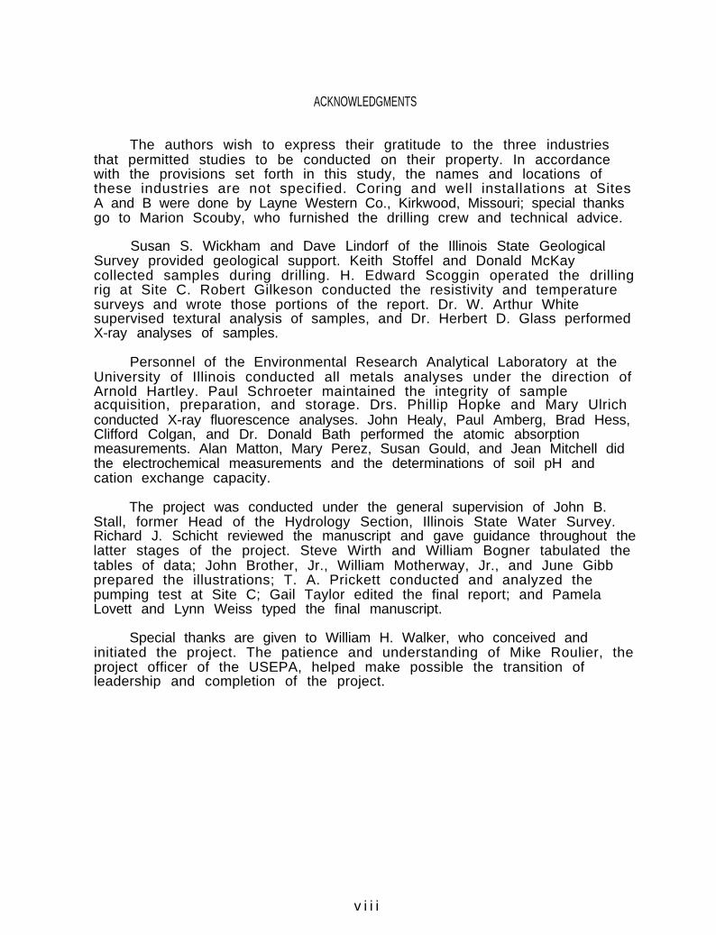
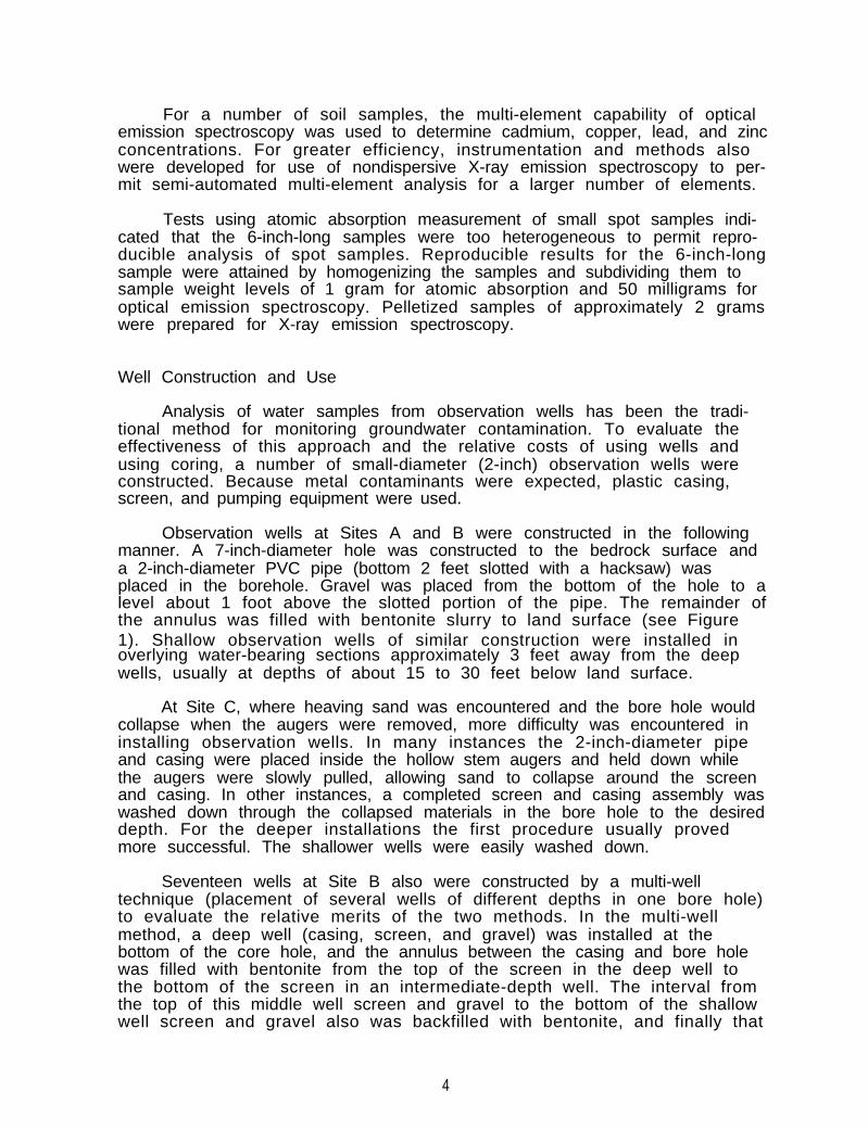
Observation wells at Sites A and B were constructed in the followingmanner. A 7-inch-diameter hole was constructed to the bedrock surface anda 2-inch-diameter PVC pipe (bottom 2 feet slotted with a hacksaw) wasplaced in the borehole. Gravel was placed from the bottom of the hole to alevel about 1 foot above the slotted portion of the pipe. The remainder ofthe annulus was filled with bentonite slurry to land surface (see Figure1). Shallow observation wells of similar construction were installed inoverlying water-bearing sections approximately 3 feet away from the deepwells, usually at depths of about 15 to 30 feet below land surface.
At Site C, where heaving sand was encountered and the bore hole wouldcollapse when the augers were removed, more difficulty was encountered ininstalling observation wells. In many instances the 2-inch-diameter pipeand casing were placed inside the hollow stem augers and held down whilethe augers were slowly pulled, allowing sand to collapse around the screenand casing. In other instances, a completed screen and casing assembly waswashed down through the collapsed materials in the bore hole to the desireddepth. For the deeper installations the first procedure usually provedmore successful. The shallower wells were easily washed down.
Seventeen wells at Site B also were constructed by a multi-welltechnique (placement of several wells of different depths in one bore hole)to evaluate the relative merits of the two methods. In the multi-wellmethod, a deep well (casing, screen, and gravel) was installed at thebottom of the core hole, and the annulus between the casing and bore holewas filled with bentonite from the top of the screen in the deep well tothe bottom of the screen in an intermediate-depth well. The interval fromthe top of this middle well screen and gravel to the bottom of the shallowwell screen and gravel also was backfilled with bentonite, and finally that
4
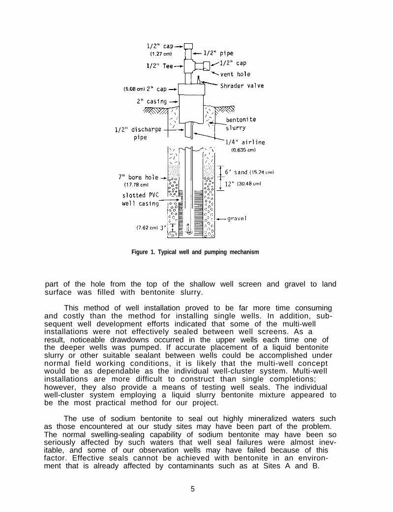
Figure 1. Typical well and pumping mechanism
part of the hole from the top of the shallow well screen and gravel to landsurface was filled with bentonite slurry.
This method of well installation proved to be far more time consumingand costly than the method for installing single wells. In addition, sub-sequent well development efforts indicated that some of the multi-wellinstallations were not effectively sealed between well screens. As aresult, noticeable drawdowns occurred in the upper wells each time one ofthe deeper wells was pumped. If accurate placement of a liquid bentoniteslurry or other suitable sealant between wells could be accomplished undernormal field working conditions, it is likely that the multi-well conceptwould be as dependable as the individual well-cluster system. Multi-wellinstallations are more difficult to construct than single completions;however, they also provide a means of testing well seals. The individualwell-cluster system employing a liquid slurry bentonite mixture appeared tobe the most practical method for our project.
The use of sodium bentonite to seal out highly mineralized waters suchas those encountered at our study sites may have been part of the problem.The normal swelling-sealing capability of sodium bentonite may have been soseriously affected by such waters that well seal failures were almost inev-itable, and some of our observation wells may have failed because of thisfactor. Effective seals cannot be achieved with bentonite in an environ-ment that is already affected by contaminants such as at Sites A and B.
5
To determine more accurately the effectiveness of bentonite as a wellsealant, an attempt was made to use strontium chloride as a tracer orindicator of well seal failure. Strontium chloride was added to the waterused to make the bentonite slurries that were placed around several wells.In theory, when the bentonite seal began to break down in a particularwell, strontium concentrations several orders of magnitude above naturallevels would be released and detected in the water samples from that well.However, this did not occur during the entire study. In fact, higherstrontium concentrations were often detected in water samples from wellswhere the bentonite seal had not been "spiked." It is possible that thesampling procedures used to collect water samples (discussed in the nextsection) flushed out any released strontium from the bentonite seal beforethe sample was taken. In any case, we were unable to determine by thistechnique if the bentonite seals had failed.
Pumping Mechanism
Observation wells were equipped with individual pumping devices tominimize possible contamination of samples from other wells. The pumpingdevices consisted of a 1/2-inch-diameter PVC discharge pipe that extendedfrom above the 2-inch well casing to the bottom of the well. A tee fittedwith short nipples and removable caps was placed at the top of this pipe(Figure 1). The cap on the vertical segment could be removed to allow forwater level measurements within the 1/2-inch pipe. The cap on the hori-zontal segment (water discharge outlet) was vented to permit stabilizationof the water level within this pipe.
A 1/4-inch plastic airline was also installed in each well. Theairline was attached to a Shrader valve at the top of the well casing andextended the entire depth of the well. The lower end of the airline wasbent up into the bottom of the 1/2-inch discharge pipe for a distance ofabout 3 inches.
Water was pumped from the wells by removing the cap from the horizon-tal portion of the 1/2-inch or 3/8-inch pipe and applying air to the systemthrough the Shrader valve. Pumping from depths as great as 70 feet waspossible with only a bicycle-type hand pump. A gasoline powered, 4-cylind-er air compressor capable of delivering about 5 cubic feet per minute atpressures up to 60 pounds per square inch (psi) also was used. An activa-ted charcoal filter was placed in the discharge airline from the compressorto insure that air from the compressor was not introducing airbornecontaminants.
Since most of the wells in this study generally had a column of waterless than 30 or 40 feet deep to be moved by the air lift mechanisms, it wasfound that operating the compressor at 20 to 25 pounds per square inch wasmost effective. Higher operating pressures caused the air bubbles to risethrough the water column instead of pushing slugs of water in front of themas desired. In the very shallow wells, less than 20 feet deep, thebicycle-type hand pump actually worked more effectively.
6
Water Sampling
Water level measurements were made and water samples were collectedfrom each well once a month. Water samples were collected in 6-ounce plas-tic containers and placed on ice until they were brought into the labora-tory, where they were refrigerated. Each well was pumped for a period oftime theoretically adequate to insure that all stored water in the wellcasing had been removed. The wells were allowed to recover, and a samplewas then collected from water that had just entered the well. This proce-dure was followed in hopes that the water sample would be representative ofthe water flowing through the aquifer at the time of collection.
Near the end of the project a brief experiment was conducted on fourwells at Site A to determine if the pumping scheme just described wasnecessary or adequate for collecting representative water samples. Wellswere selected on the basis of early results of chemical analyses of watersamples collected. Zinc concentrations in water from the four wells hadranged from 6.2 to 25.9 mg/l, 300 to 790 mg/l, 342 to 850 mg/l, and 12,700to 21,580 mg/l, respectively. These values represent fluctuations in zinccontent of 76, 62, 60, and 42 percent using the higher values as baseconcentrations.
To determine if these fluctuations were real or a function of thesampling procedure, the following experiment was conducted. Water levelmeasurements were taken in each well and the volumes of water stored in the2-inch-diameter casings and screens were calculated. Pumping was initiatedand samples were collected just after pumping began and at increments ofone-half the total stored water volume until a total of 5 volumes had beenpumped.
Figure 2 illustrates the results of these tests for the four wells.Percentage decreases in zinc concentrations from the first sample to thelast ranged from about 45 to 78 percent with the greatest decreasesoccurring in the wells with the lowest zinc concentrations. Reductions inzinc content at the 1 volume pumped stage (the procedure followed in oursampling program) ranged from about 18 to 46 percent. This suggests thatall of the zinc determinations of water samples collected could be as muchas 30 percent higher than the stabilized zinc content beyond the 5-volumepumped stage. If the sampling procedure employed varied by even as littleas 50 percent, pumping only one-half or one and one-half the stored volume,it could account for as much as 15 to 20 percent of the fluctuations in thesample results.
Additional experiments of this type should be undertaken to designsatisfactory sampling procedures for other chemicals. Further, theseexperiments should be done at the beginning of a project as opposed to nearthe end as in this case. The results of these brief tests were the impetusfor later work conducted by Gibb et al. (1981). Results of that workindicate that sampling for metals should not be attempted with the type ofair-lift mechanism employed in this project. The metals content of samplescollected with this mechanism is likely to be lower than that of water inthe formation being sampled.
7
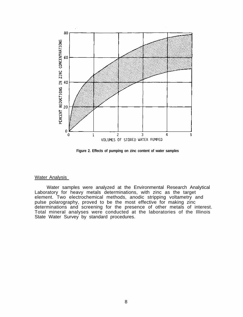
Figure 2. Effects of pumping on zinc content of water samples
Water Analysis
Water samples were analyzed at the Environmental Research AnalyticalLaboratory for heavy metals determinations, with zinc as the targetelement. Two electrochemical methods, anodic stripping voltametry andpulse polarography, proved to be the most effective for making zincdeterminations and screening for the presence of other metals of interest.Total mineral analyses were conducted at the laboratories of the IllinoisState Water Survey by standard procedures.
8
SECTION 3
SUPPLEMENTAL FIELD TECHNIQUES
Early in an investigation of groundwater contamination problems it isessential to have information on geologic conditions in the region. Defi-nition of the groundwater flow system also is important. Because largeareas and considerable depths may be involved, gathering this informationthrough a systematic drilling program may be economically unfeasible.
Geologists and engineers are making increased use of geophysicalmethods to rapidly determine shallow geologic conditions. Two of thesegeophysical methods, the measurement of electrical earth resistivity andthe measurement of soil temperature, are useful for economic, rapidinvestigation of geologic conditions related to groundwater contamination.These geophysical methods can provide information on the regional variationof the lithologic character of the shallow geologic materials. They alsocan provide information on the shallow groundwater flow system and possiblycan define zones of degraded water quality within the flow system.
Electrical Earth Resistivity Methods
A comprehensive review of the theory and interpretation of electricalearth resistivity is presented by Van Nostrand and Cook (1966). The use ofelectrical earth resistivity methods in groundwater contamination studiesis discussed in many papers. Cartwright and Sherman (1972) discuss resis-tivity methods as useful tools in locating suitable sanitary landfill sitesand in monitoring the effect of a refuse disposal site on a shallow ground-water systems. Berk and Yare (1977) describe a case in which groundwatercontamination problems were caused by disposal of industrial process waterinto an unlined lagoon in permeable sediments. They tell how electricalearth resistivity methods were used successfully to define zones ofdegraded water quality and to locate sites for monitoring wells.
A common approach for making electrical earth resistivity measurementsis to use the Wenner configuration, where four electrodes are spacedequally along a straight line. Through systematic enlargement of thedistance (a-spacing) between electrodes, the electrical field is expandedto include a greater volume'of earth materials. The value of the apparentresistivity obtained at each a-spacing approximates the average of the trueresistivity of all the materials within the impressed field. The apparentresistivity depth profile generated at a location by taking measurements atseveral a-spacings can be reduced analytically to determine the number oflayers of geologic material present and the thickness and true resistivityof each layer.
The fundamental factors that govern resistance to the flow of electri-cal current through earth materials are: a) water saturation, b) mineralcontent of the water, and c) geologic factors.
The presence of water is important to the conductance of an electriccurrent through earth materials. In general, saturated materials have a
9
higher conductivity (lower apparent resistivity) than similar unsaturatedmaterials.
The mineral content of the water present in earth materials is a majorcontrolling factor of the conductance of electrical current through thematerial. As the ionic content of the water increases, the apparentresistivity of the earth material decreases.
There are two geologic factors which affect apparent resistivityvalues. One of these, the "formation factor," relates to the porosity ofthe earth material as well as the shape of the pores and the manner inwhich they are interconnected. A second geologic factor which affectsapparent resistivity is the presence of conductive solids such as clayminerals. An increase in the amount of clay minerals present in an earthmaterial will lower the apparent resistivity of that material. Generally,fine-grained clayey sediments have lower apparent resistivities than clean,coarse sands and gravels.
An electrical earth resistivity survey was made at Site A to determinethe applicability of this technique. The results of that work aredescribed in the case history of Site A.
Temperature Surveys
The distribution of temperature within the lithosphere can be signifi-cantly affected by the movement of groundwater. Cartwright (1968) usedsoil temperatures to locate shallow aquifers and discussed (1974) the useof soil temperature to trace shallow groundwater flow systems. There islimited published information on the application of soil temperatures as atool for investigation of groundwater contamination problems. Cartwrightand McComas (1968) used soil temperature measurements in the vicinity oftwo sanitary landfills to map shallow groundwater flow systems anddischarges of leachate.
In field investigations, soil temperature measurements are commonlymade with a thermistor at the tip of an insulated probe. The probe can beinserted into the soil to any desired depth. Measurements are usually madeat depths greater than 19.7 inches to eliminate diurnal temperaturevariations. Temperatures are read after the probe comes into equilibriumwith the soil, roughly after about 5 minutes.
Factors which affect the temperature of the soils in the flow systeminclude the velocity of groundwater movement, the vertical or lateraldirection of groundwater movement, lithology of the geologic materialswhich affects their thermal properties, heating effects due to land cover,and geothermal heat added to the system.
Human activities can serve as sources of heat which affect local soiltemperatures. Cartwright and Reed (1972) measured anomalous high soiltemperatures in the vicinity of a village. Heat generated at industrialsites may have a significant effect on soil temperatures locally, with thedistribution of this heat related to the shallow groundwater flow system inthe vicinity of the site.
10
Soil temperature surveys were made at all sites to test the applica-bility of this method.
Infrared Photography
Infrared aerial photographs of Sites A and B were taken in the earlypart of October 1974 by the National Environmental Research Center - LasVegas, U.S. Environmental Protection Agency. Another round of flights wasmade in June 1975. Examination of these photos provided very little infor-mation concerning the groundwater conditions or effects of groundwaterpollution at these sites.
The photos were helpful however in detecting past effects of wind-blown pollutants and surface water movement of pollutants. Dr. William R.Edwards, Illinois State Natural History Survey, found the photos useful inconducting a preliminary study of the plant life at Site A. A brief des-cription of his results is included in the case history of Site A.
11
SECTION 4
SITES USED IN THE STUDY
Three industrial complexes (Sites A, B, and C) were selected for astudy of the effects of waste disposal on soils and shallow groundwatersystems.
Two sites (A and B) located in moraine and ridged drift areas ofsouth-central Illinois initially were selected for study on the basis ofgeology, the types and quantities of waste generated, and the manner ofdisposal. It was thought desirable to study areas where the unconsolidatedmaterials are relatively thin (less than 50 to 75 feet) and underlain byPennsylvanian age shales. Special emphasis was also given to sites whereglacial materials were predominantly low-permeability clays, silts, andtills. Such sites theoretically would be desirable for disposal activitieswith little resulting groundwater contamination.
To determine the general applicability of the coring technique as amonitoring tool, a third site (C) located in a sandy alluvium environmentin north-central Illinois (presumably undesirable for disposal activity)was chosen later. Sites A, B, and C are secondary zinc smelting plantsthat have generated large volumes of metals-rich waste material over manyyears of operations. Most of this waste has been in the form of cindersthat have been piled on or spread over the plant properties as fillmaterial.
The selection of sites to be studied ultimately is decided by indus-trial politics. Because of the necessity of releasing all data collectedduring a study, it is often difficult to convince the officers of an indus-try of the merits of a study. In most cases the company involved has verylittle to gain and the potential for great losses (bad publicity, regula-tory action by state and federal government, or the discovery of unknownproblems). In the planning of any proposed research, it is recommendedthat written permission be obtained from the appropriate industrial offi-cers to insure that the desired sites can in fact be studied.
Regional Geology
The areas of study in this project all are underlain by varying thick-nesses of unconsolidated materials of Pleistocene age over bedrock. Duringthe Pleistocene, four major periods of glacial advance (Nebraskan, Kansan,Illinoian, and Wisconsinan) occurred in Illinois. These periods were sepa-rated by interglacial episodes of soil formation (Aftonian, Yarmouthian,and Sangamonian Stages). Figure 3 illustrates the regional distribution ofinterglacial episodes in Il l inois. Figure 4 indicates the time relation-ships of the glacial periods, unconsolidated sediments (rock stratigraphy),and soil development in Illinois.
The Nebraskan glacial advance represented the first episode ofPleistocene glaciation in Illinois and covered a relatively small portionof western Illinois, resulting in a scarcity of Nebraskan-age glacial
12
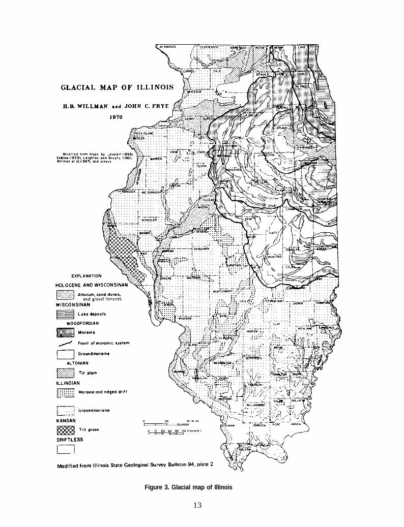
Figure 3. Glacial map of Illinois
13
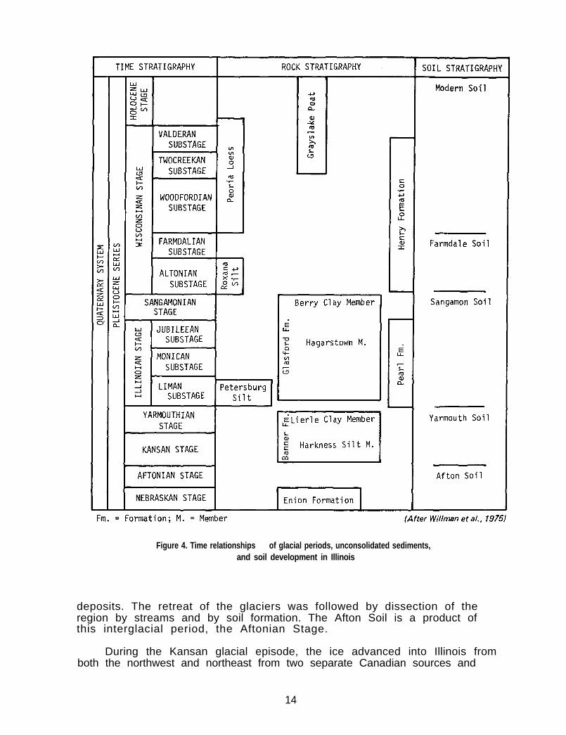
Figure 4. Time relationships of glacial periods, unconsolidated sediments,and soil development in Illinois
deposits. The retreat of the glaciers was followed by dissection of theregion by streams and by soil formation. The Afton Soil is a product ofthis interglacial period, the Aftonian Stage.
During the Kansan glacial episode, the ice advanced into Illinois fromboth the northwest and northeast from two separate Canadian sources and
14
covered about two-thirds of Illinois. The Yarmouth Soil profile whichdeveloped on the Kansan glacial deposits after the retreat of the ice isquite thick, suggesting a long period of soil formation.
The Illinoian Stage was marked by three major glacial advances intoIllinois from the northeast, which covered most of the state. The SangamonSoil developed on the Illinoian deposits following the retreat of the icesheets. Local accumulation of predominantly fine-grained sediments inpoorly drained areas also developed on the landscape.
There were two glacial advances into Illinois during the WisconsinanStage. Glacial deposits were limited to northern Illinois, with largequantities of wind-blown silt, called loess, deposited over much of therest of the state. The two advances were separated by an interval of soilformation which produced the Farmdale Soil. Radiocarbon dating indicatesthat the retreat of glaciers from Illinois was about 12,000 years ago. TheModern Soil has been developed on the surficial glacial deposits from thattime to the present.
Stratigraphy
Soil formation is characterized by a number of processes, which, overa period of time, tend to result in the development of three soil zones orhorizons. Organic material accumulates in the upper zone or A horizon andthe parent material is broken down by weathering, forming soluble mineralsand collodial suspensions which are leached from the A horizon and moved toor throuqh the underlyinq zone, the B horizon. Clay minerals and iron andmanganese commonly are transported downward and deposited in the B horizon.The B horizon also is characterized by increasing color segregation ormottling due to alternating wet and dry conditions. The organic A horizonoften is considered the zone of depletion while the B horizon is the zoneof accumulation.
Carbonates are leached from the A and B horizons and usually arecarried downward in the pore water into the groundwater system. In somecases, carbonate minerals accumulate in or precipitate from the pore waterat the top of the lowest horizon, the C horizon, which is commonly calledthe parent material.
The preglacial bedrock surface in Illinois varies in age fromPennsylvanian to Cambrian. All sites studied are underlain by Pennsyl-vanian age rocks consisting predominantly of shale interbedded with thinsandstone, limestone, and coal layers.
Sites A and B are located in south-central Illinois in relatively flatand featureless drift plains underlain by till sheets of Kansan andIllinoian age, Illinoian water-laid deposits, and Wisconsinan loess andsilts (see Figure 3). Site C is located in north-central Illinois on thefloodplain of the Illinois River and is underlain by recent alluvialmaterials over Wisconsinan glacial outwash (Figure 3). The stratigraphy ofall three sites is described in detail in the following case historysections.
15
SECTION 5
CASE HISTORIES
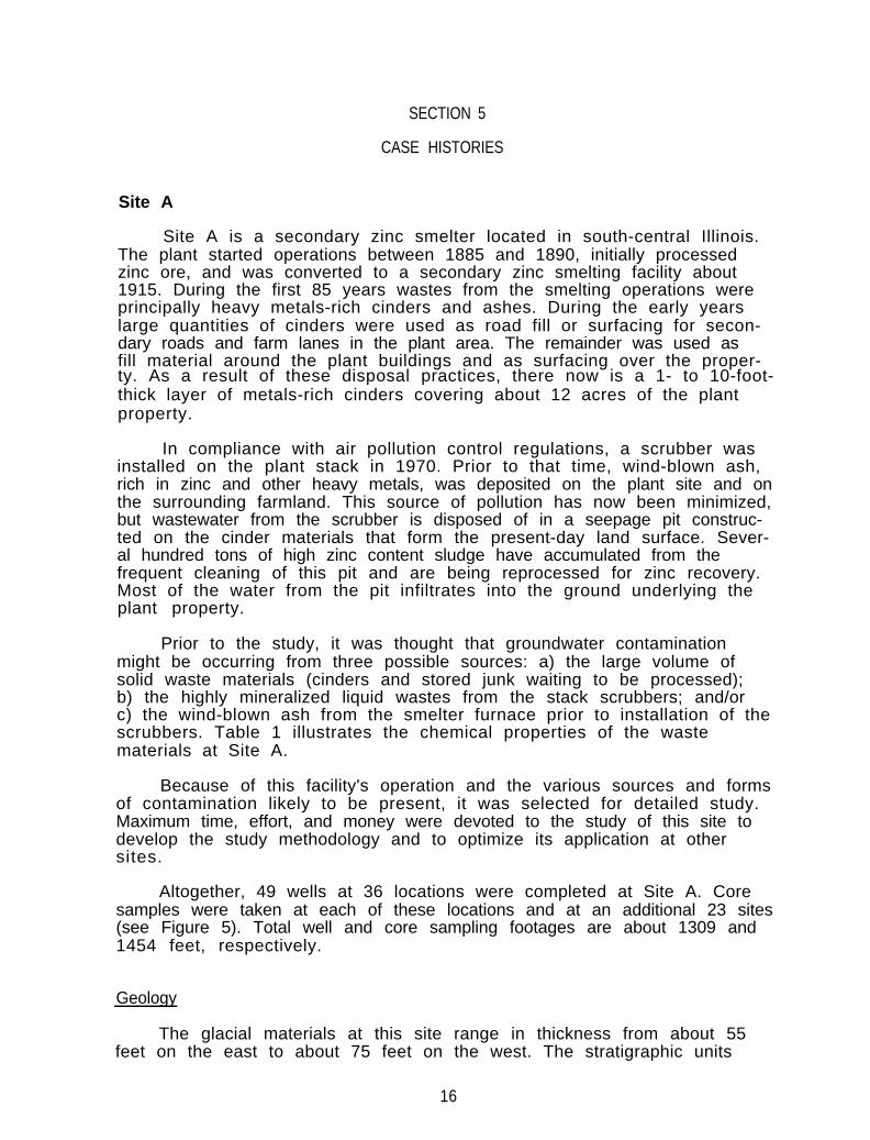
Site A
Site A is a secondary zinc smelter located in south-central Illinois.The plant started operations between 1885 and 1890, initially processedzinc ore, and was converted to a secondary zinc smelting facility about1915. During the first 85 years wastes from the smelting operations wereprincipally heavy metals-rich cinders and ashes. During the early yearslarge quantities of cinders were used as road fill or surfacing for secon-dary roads and farm lanes in the plant area. The remainder was used asfill material around the plant buildings and as surfacing over the proper-ty. As a result of these disposal practices, there now is a 1- to 10-foot-thick layer of metals-rich cinders covering about 12 acres of the plantproperty.
In compliance with air pollution control regulations, a scrubber wasinstalled on the plant stack in 1970. Prior to that time, wind-blown ash,rich in zinc and other heavy metals, was deposited on the plant site and onthe surrounding farmland. This source of pollution has now been minimized,but wastewater from the scrubber is disposed of in a seepage pit construc-ted on the cinder materials that form the present-day land surface. Sever-al hundred tons of high zinc content sludge have accumulated from thefrequent cleaning of this pit and are being reprocessed for zinc recovery.Most of the water from the pit infiltrates into the ground underlying theplant property.
Prior to the study, it was thought that groundwater contaminationmight be occurring from three possible sources: a) the large volume ofsolid waste materials (cinders and stored junk waiting to be processed);b) the highly mineralized liquid wastes from the stack scrubbers; and/orc) the wind-blown ash from the smelter furnace prior to installation of thescrubbers. Table 1 illustrates the chemical properties of the wastematerials at Site A.
Because of this facility's operation and the various sources and formsof contamination likely to be present, it was selected for detailed study.Maximum time, effort, and money were devoted to the study of this site todevelop the study methodology and to optimize its application at othersites.
Altogether, 49 wells at 36 locations were completed at Site A. Coresamples were taken at each of these locations and at an additional 23 sites(see Figure 5). Total well and core sampling footages are about 1309 and1454 feet, respectively.
Geology
The glacial materials at this site range in thickness from about 55feet on the east to about 75 feet on the west. The stratigraphic units
16
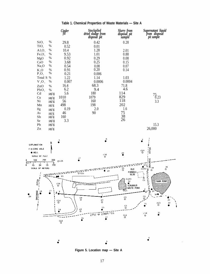
Table 1. Chemical Properties of Waste Materials — Site A
SiO2%
TiO2%
Al2O 3%
Fe2O 3%
MgO %CaO %Na2O %K 2O %P 2O 5
%Total S %V 2O 5 %ZnO %PbO 2 %Cd µg/gCu µg/gNi µg/gMn µg/gHg µg/gAs µg/gSb µg/gSe µg/gPb µg/gZn µg/g
Slurry fromdisposal pit
sample0.28
Supernatant liquidfrom disposal
pit sample
Cinderfill
Stockpileddried sludge from
disposal pit0.420.011.281.010.290.250.080.200.0061.140.0006
68.39.4
1801079
160198
2.090
29.80.52
10.49.530.923.680.540.910.211.220.007
16.46.25.6
101056
4980.19
46160
3.3
2.010.880.080.150.070.14
1.030.0004
71.84.6
114829118202
1.6753826
750.233.3
15.326,000
Figure 5. Location map — Site A
17
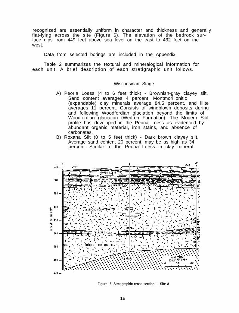
recognized are essentially uniform in character and thickness and generallyflat-lying across the site (Figure 6). The elevation of the bedrock sur-face dips from 449 feet above sea level on the east to 432 feet on thewest.
Data from selected borings are included in the Appendix.
Table 2 summarizes the textural and mineralogical information foreach unit. A brief description of each stratigraphic unit follows.
Wisconsinan Stage
A) Peoria Loess (4 to 6 feet thick) - Brownish-gray clayey silt.Sand content averages 4 percent. Montmorillonitic(expandable) clay minerals average 84.5 percent, and illiteaverages 11 percent. Consists of windblown deposits duringand following Woodfordian glaciation beyond the limits ofWoodfordian glaciation (Wedron Formation). The Modern Soilprofile has developed in the Peoria Loess as evidenced byabundant organic material, iron stains, and absence ofcarbonates.
B) Roxana Silt (0 to 5 feet thick) - Dark brown clayey silt.Average sand content 20 percent, may be as high as 34percent. Similar to the Peoria Loess in clay mineral
Figure 6. Stratigraphic cross section — Site A
18
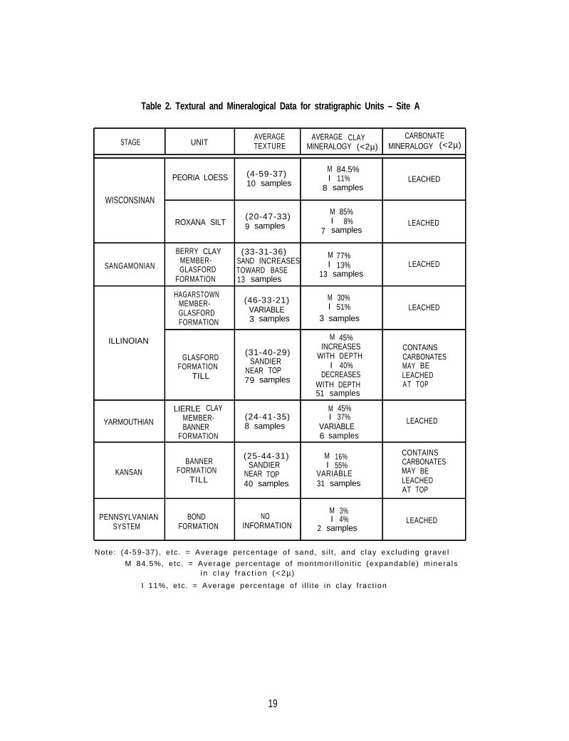
Table 2. Textural and Mineralogical Data for stratigraphic Units – Site A
CARBONATESTAGE
AVERAGEUNIT
AVERAGE CLAYTEXTURE MINERALOGY (<2µ) MINERALOGY (<2µ)
M 84.5%PEORIA LOESS (4-59-37)
10I 11% LEACHEDsamples
8 samples
WISCONSINAN
(20-47-33)M 85%
ROXANA SILT 9I 8%samples LEACHED
7 samples
BERRY CLAY (33-31-36) M 77%SANGAMONIAN
MEMBER- SAND INCREASES I 13% LEACHEDGLASFORD TOWARD BASE
FORMATION13
13samples
samples
HAGARSTOWN M 30%MEMBER- (46-33-21)
I 51% LEACHEDGLASFORD VARIABLE
FORMATION 3 samples 3 samples
ILLINOIAN M 45%
(31-40-29)INCREASES CONTAINS
GLASFORD WITH DEPTHSANDIER CARBONATES
FORMATION I 40%NEAR TOP MAY BE
TILL 79DECREASES LEACHEDsamples
WITH DEPTH A T TOP51 samples
LIERLE CLAY M 45%
YARMOUTHIAN MEMBER- (24-41-35) I 37%BANNER
LEACHED8 samples VARIABLE
FORMATION 6 samples
(25-44-31) M 16% CONTAINSBANNER SANDIER I 55% CARBONATES
KANSAN FORMATION NEAR TOP MAYVARIABLE BETILL 40 samples 31 LEACHEDsamples
AT TOP
M 3%PENNSYLVANIAN BOND NO I 4% LEACHED
SYSTEM FORMATION INFORMATION 2 samples
Note: (4-59-37), etc. = Average percentage of sand, s i l t , and c lay excluding gravel
M 84.5%, etc. = Average percentage of montmor i l loni t ic (expandable) mineralsi n c l a y f r a c t i o n ( < 2 µ )
I 11%, etc. = Average percentage of i l l i te in c lay f ract ion
19
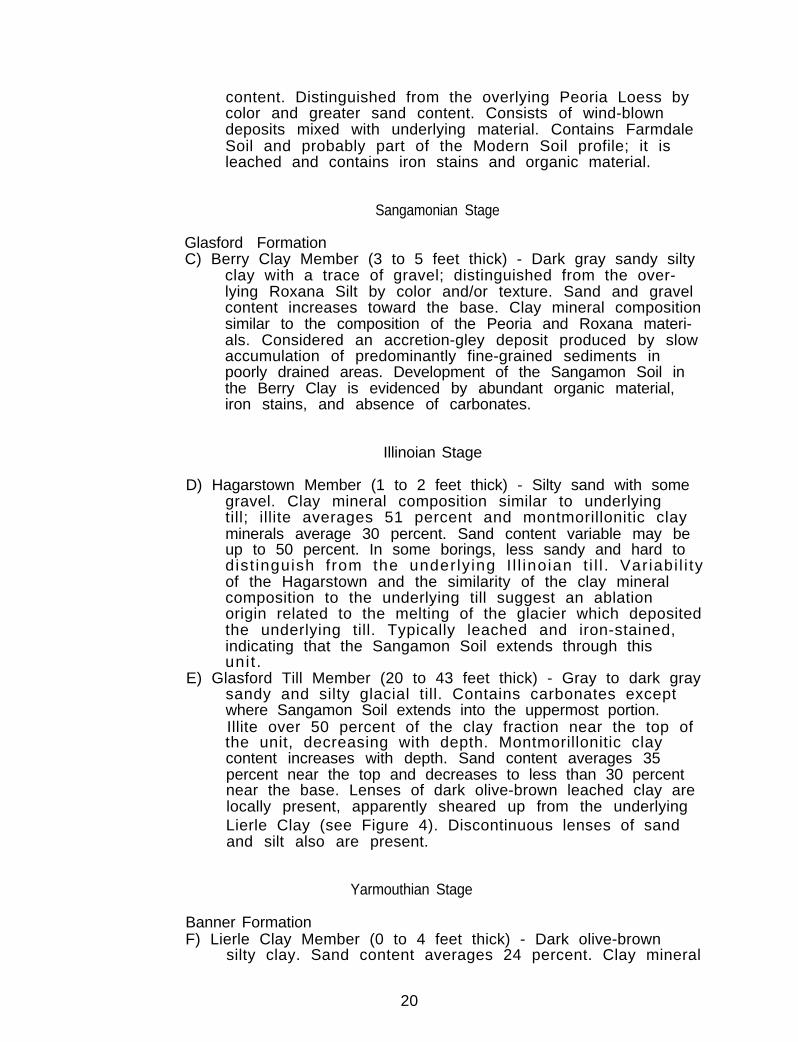
content. Distinguished from the overlying Peoria Loess bycolor and greater sand content. Consists of wind-blowndeposits mixed with underlying material. Contains FarmdaleSoil and probably part of the Modern Soil profile; it isleached and contains iron stains and organic material.
Sangamonian Stage
Glasford FormationC) Berry Clay Member (3 to 5 feet thick) - Dark gray sandy silty
clay with a trace of gravel; distinguished from the over-lying Roxana Silt by color and/or texture. Sand and gravelcontent increases toward the base. Clay mineral compositionsimilar to the composition of the Peoria and Roxana materi-als. Considered an accretion-gley deposit produced by slowaccumulation of predominantly fine-grained sediments inpoorly drained areas. Development of the Sangamon Soil inthe Berry Clay is evidenced by abundant organic material,iron stains, and absence of carbonates.
Illinoian Stage
D) Hagarstown Member (1 to 2 feet thick) - Silty sand with somegravel. Clay mineral composition similar to underlyingtill; illite averages 51 percent and montmorillonitic clayminerals average 30 percent. Sand content variable may beup to 50 percent. In some borings, less sandy and hard todist inguish from the underlying I l l inoian t i l l . Variabi l i tyof the Hagarstown and the similarity of the clay mineralcomposition to the underlying till suggest an ablationorigin related to the melting of the glacier which depositedthe underlying till. Typically leached and iron-stained,indicating that the Sangamon Soil extends through thisunit .
E) Glasford Till Member (20 to 43 feet thick) - Gray to dark graysandy and silty glacial till. Contains carbonates exceptwhere Sangamon Soil extends into the uppermost portion.Illite over 50 percent of the clay fraction near the top ofthe unit, decreasing with depth. Montmorillonitic claycontent increases with depth. Sand content averages 35percent near the top and decreases to less than 30 percentnear the base. Lenses of dark olive-brown leached clay arelocally present, apparently sheared up from the underlyingLierle Clay (see Figure 4). Discontinuous lenses of sandand silt also are present.
Yarmouthian Stage
Banner FormationF) Lierle Clay Member (0 to 4 feet thick) - Dark olive-brown
silty clay. Sand content averages 24 percent. Clay mineral
20
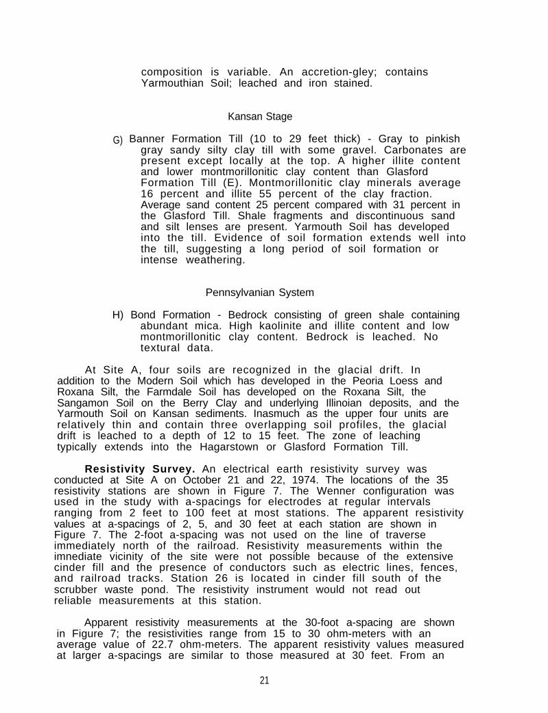
composition is variable. An accretion-gley; containsYarmouthian Soil; leached and iron stained.
G)
Kansan Stage
Banner Formation Till (10 to 29 feet thick) - Gray to pinkishgray sandy silty clay till with some gravel. Carbonates arepresent except locally at the top. A higher illite contentand lower montmorillonitic clay content than GlasfordFormation Till (E). Montmorillonitic clay minerals average16 percent and illite 55 percent of the clay fraction.Average sand content 25 percent compared with 31 percent inthe Glasford Till. Shale fragments and discontinuous sandand silt lenses are present. Yarmouth Soil has developedinto the till. Evidence of soil formation extends well intothe till, suggesting a long period of soil formation orintense weathering.
Pennsylvanian System
H) Bond Formation - Bedrock consisting of green shale containingabundant mica. High kaolinite and illite content and lowmontmorillonitic clay content. Bedrock is leached. Notextural data.
At Site A, four soils are recognized in the glacial drift. Inaddition to the Modern Soil which has developed in the Peoria Loess andRoxana Silt, the Farmdale Soil has developed on the Roxana Silt, theSangamon Soil on the Berry Clay and underlying Illinoian deposits, and theYarmouth Soil on Kansan sediments. Inasmuch as the upper four units arerelatively thin and contain three overlapping soil profiles, the glacialdrift is leached to a depth of 12 to 15 feet. The zone of leachingtypically extends into the Hagarstown or Glasford Formation Till.
Resistivity Survey. An electrical earth resistivity survey wasconducted at Site A on October 21 and 22, 1974. The locations of the 35resistivity stations are shown in Figure 7. The Wenner configuration wasused in the study with a-spacings for electrodes at regular intervalsranging from 2 feet to 100 feet at most stations. The apparent resistivityvalues at a-spacings of 2, 5, and 30 feet at each station are shown inFigure 7. The 2-foot a-spacing was not used on the line of traverseimmediately north of the railroad. Resistivity measurements within theimnediate vicinity of the site were not possible because of the extensivecinder fill and the presence of conductors such as electric lines, fences,and railroad tracks. Station 26 is located in cinder fill south of thescrubber waste pond. The resistivity instrument would not read outreliable measurements at this station.
Apparent resistivity measurements at the 30-foot a-spacing are shownin Figure 7; the resistivities range from 15 to 30 ohm-meters with anaverage value of 22.7 ohm-meters. The apparent resistivity values measuredat larger a-spacings are similar to those measured at 30 feet. From an
21
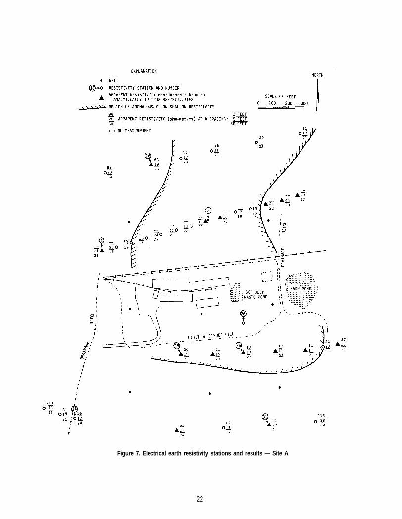
Figure 7. Electrical earth resistivity stations and results — Site A
22
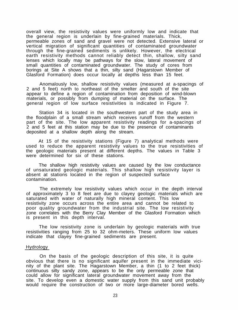
overall view, the resistivity values were uniformly low and indicate thatthe general region is underlain by fine-grained materials. Thick,permeable zones of sand and gravel were not detected. Extensive lateral orvertical migration of significant quantities of contaminated groundwaterthrough the fine-grained sediments is unlikely. However, the electricalearth resistivity methods cannot reliably detect thin, shallow, silty sandlenses which locally may be pathways for the slow, lateral movement ofsmall quantities of contaminated groundwater. The study of cores fromborings at Site A shows that a thin, silty sand (Hagarstown Member ofGlasford Formation) does occur locally at depths less than 15 feet.
Anomalously low, shallow resistivity values (measured at a-spacings of2 and 5 feet) north to northeast of the smelter and south of the siteappear to define a region of contamination from deposition of wind-blownmaterials, or possibly from dumping of material on the surface. Thegeneral region of low surface resistivities is indicated in Figure 7.
Station 34 is located in the southwestern part of the study area inthe floodplain of a small stream which receives runoff from the westernpart of the site. The low apparent resistivity readings for a-spacings of2 and 5 feet at this station may be due to the presence of contaminantsdeposited at a shallow depth along the stream.
At 15 of the resistivity stations (Figure 7) analytical methods wereused to reduce the apparent resistivity values to the true resistivities ofthe geologic materials present at different depths. The values in Table 3were determined for six of these stations.
The shallow high resistivity values are caused by the low conductanceof unsaturated geologic materials. This shallow high resistivity layer isabsent at stations located in the region of suspected surfacecontamination.
The extremely low resistivity values which occur in the depth intervalof approximately 3 to 8 feet are due to clayey geologic materials which aresaturated with water of naturally high mineral content. This lowresistivity zone occurs across the entire area and cannot be related topoor quality groundwater from the industrial site. The low resistivityzone correlates with the Berry Clay Member of the Glasford Formation whichis present in this depth interval.
The low resistivity zone is underlain by geologic materials with trueresistivities ranging from 25 to 32 ohm-meters. These uniform low valuesindicate that clayey fine-grained sediments are present.
Hydrology
On the basis of the geologic description of this site, it is quiteobvious that there is no significant aquifer present in the immediate vici-nity of the plant site. The Hagarstown Member, a thin (1 to 2 feet thick)continuous silty sandy zone, appears to be the only permeable zone thatcould allow for significant lateral groundwater movement away from thesite. To develop even a domestic water supply from this sand unit probablywould require the construction of two or more large-diameter bored wells.
23
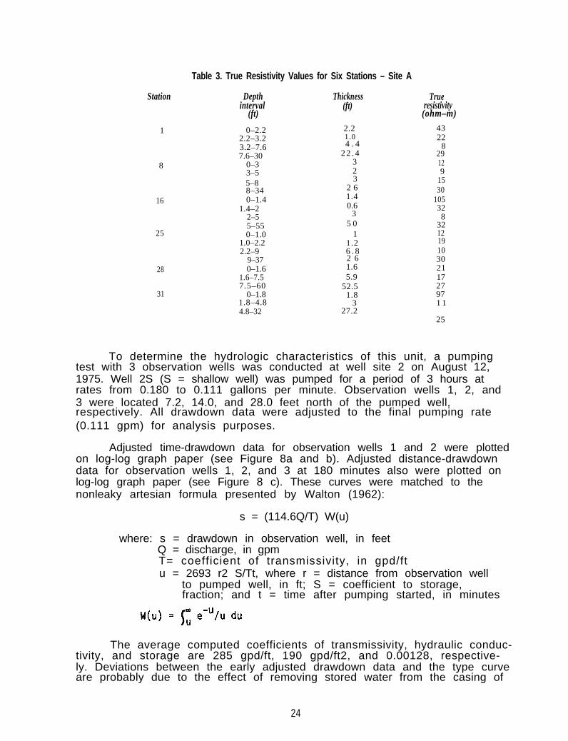
Table 3. True Resistivity Values for Six Stations – Site A
Station Depthinterval
(ft)
Thickness(ft)
2.21.04 . 4
Trueresistivity(ohm–m)
0–2.212.2–3.23.2–7.6
2 6
2 2 . 4
1.4
3–58
7.6–300–3
4322
829129
1530
10532
2–5 85–55 32
121910
9–37 30211727971 1
25
323
0.63
0–1.416
5–88–34
1.4–2
5 0125 0–1.0
1.0–2.2 1.26 . 82 6
7.5–60
1.6
0–1.8
28
2.2–9
1.8–4.831
0–1.61.6–7.5 5.9
4.8–32
52.51.8
327.2
To determine the hydrologic characteristics of this unit, a pumpingtest with 3 observation wells was conducted at well site 2 on August 12,1975. Well 2S (S = shallow well) was pumped for a period of 3 hours atrates from 0.180 to 0.111 gallons per minute. Observation wells 1, 2, and3 were located 7.2, 14.0, and 28.0 feet north of the pumped well,respectively. All drawdown data were adjusted to the final pumping rate(0.111 gpm) for analysis purposes.
Adjusted time-drawdown data for observation wells 1 and 2 were plottedon log-log graph paper (see Figure 8a and b). Adjusted distance-drawdowndata for observation wells 1, 2, and 3 at 180 minutes also were plotted onlog-log graph paper (see Figure 8 c). These curves were matched to thenonleaky artesian formula presented by Walton (1962):
s = (114.6Q/T) W(u)
where: s = drawdown in observation well, in feetQ = discharge, in gpmT= coefficient of transmissivity, in gpd/ftu = 2693 r2 S/Tt, where r = distance from observation well
to pumped well, in ft; S = coefficient to storage,fraction; and t = time after pumping started, in minutes
The average computed coefficients of transmissivity, hydraulic conduc-tivity, and storage are 285 gpd/ft, 190 gpd/ft2, and 0.00128, respective-ly. Deviations between the early adjusted drawdown data and the type curveare probably due to the effect of removing stored water from the casing of
24
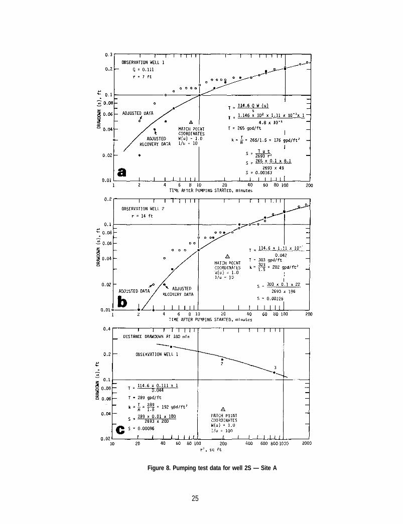
Figure 8. Pumping test data for well 2S — Site A
25
the pumped well. For this reason, heavy emphasis was placed on matchingrecovery data and late pumpage data to the type curve.
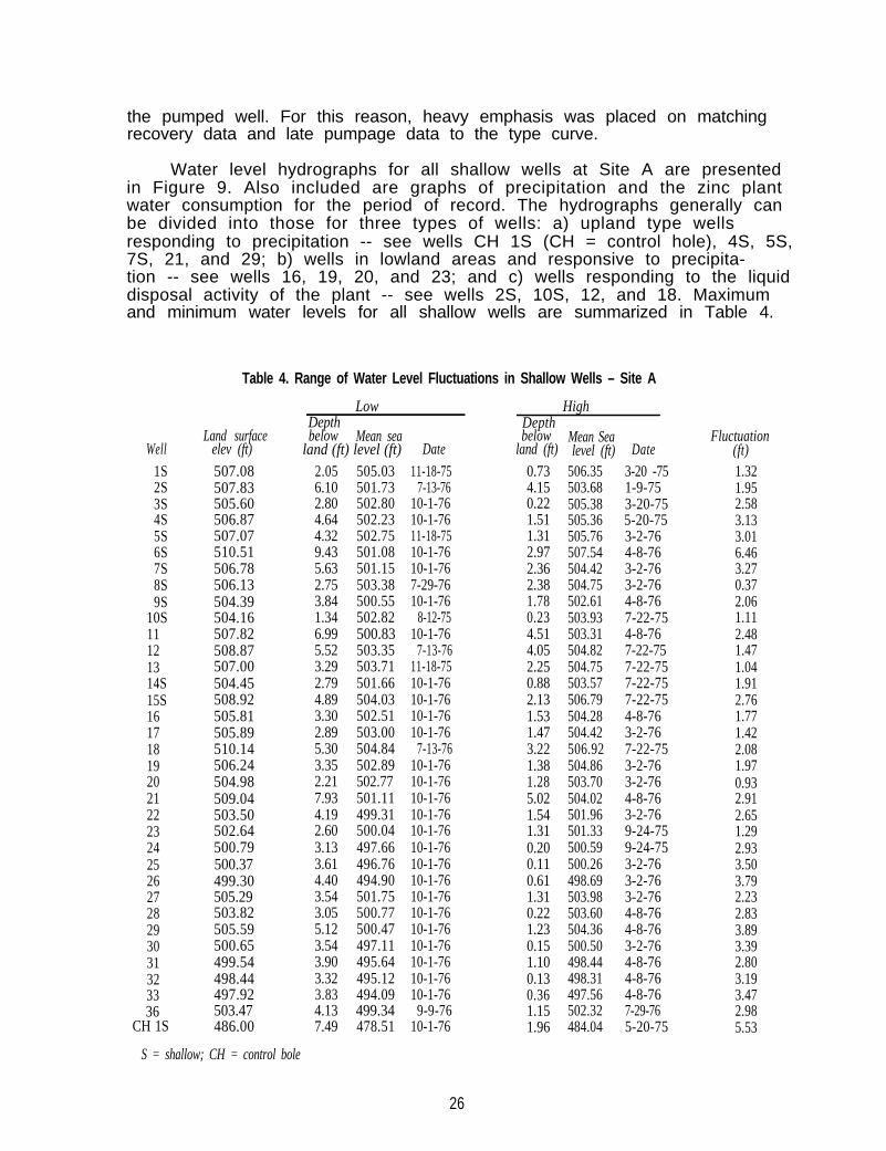
Water level hydrographs for all shallow wells at Site A are presentedin Figure 9. Also included are graphs of precipitation and the zinc plantwater consumption for the period of record. The hydrographs generally canbe divided into those for three types of wells: a) upland type wellsresponding to precipitation -- see wells CH 1S (CH = control hole), 4S, 5S,7S, 21, and 29; b) wells in lowland areas and responsive to precipita-tion -- see wells 16, 19, 20, and 23; and c) wells responding to the liquiddisposal activity of the plant -- see wells 2S, 10S, 12, and 18. Maximumand minimum water levels for all shallow wells are summarized in Table 4.
Table 4. Range of Water Level Fluctuations in Shallow Wells – Site A
Well
1S2S3S4S5S6S7S8S9S
10S11121314S15S16171819202122232425262728293031323336
CH 1S
Land surfaceelev (ft)
507.08507.83505.60506.87507.07510.51506.78506.13504.39504.16507.82508.87507.00504.45508.92505.81505.89510.14506.24504.98509.04503.50502.64500.79500.37499.30505.29503.82505.59500.65499.54498.44497.92503.47486.00
LowDepthbelow Mean sea
land (ft) level (ft) Date
2.05 505.03 11-18-756.10 501.73 7-13-762.80 502.80 10-1-764.64 502.23 10-1-764.32 502.75 11-18-759.43 501.08 10-1-765.63 501.15 10-1-762.75 503.38 7-29-763.84 500.55 10-1-761.34 502.82 8-12-756.99 500.83 10-1-765.52 503.35 7-13-763.29 503.71 11-18-752.79 501.66 10-1-764.89 504.03 10-1-763.30 502.51 10-1-762.89 503.00 10-1-765.30 504.84 7-13-763.35 502.89 10-1-762.21 502.77 10-1-767.93 501.11 10-1-764.19 499.31 10-1-762.60 500.04 10-1-763.13 497.66 10-1-763.61 496.76 10-1-764.40 494.90 10-1-763.54 501.75 10-1-763.05 500.77 10-1-765.12 500.47 10-1-763.54 497.11 10-1-763.90 495.64 10-1-763.32 495.12 10-1-763.83 494.09 10-1-764.13 499.34 9-9-767.49 478.51 10-1-76
Depthbelow
land (ft)
0.734.150.221.511.312.972.362.381.780.234.514.052.250.882.131.531.473.221.381.285.021.541.310.200.110.611.310.221.230.151.100.130.361.151.96
High
Mean Sea Fluctuationlevel (ft) Date (ft)
506.35 3-20 -75 1.32503.68 1-9-75 1.95505.38 3-20-75 2.58505.36 5-20-75 3.13505.76 3-2-76 3.01507.54 4-8-76 6.46504.42 3-2-76 3.27504.75 3-2-76 0.37502.61 4-8-76 2.06503.93 7-22-75 1.11503.31 4-8-76 2.48504.82 7-22-75 1.47504.75 7-22-75 1.04503.57 7-22-75 1.91506.79 7-22-75 2.76504.28 4-8-76 1.77504.42 3-2-76 1.42506.92 7-22-75 2.08504.86 3-2-76 1.97503.70 3-2-76 0.93504.02 4-8-76 2.91501.96 3-2-76 2.65501.33 9-24-75 1.29500.59 9-24-75 2.93500.26 3-2-76 3.50498.69 3-2-76 3.79503.98 3-2-76 2.23503.60 4-8-76 2.83504.36 4-8-76 3.89500.50 3-2-76 3.39498.44 4-8-76 2.80498.31 4-8-76 3.19497.56 4-8-76 3.47502.32 7-29-76 2.98484.04 5-20-75 5.53
S = shallow; CH = control bole
26
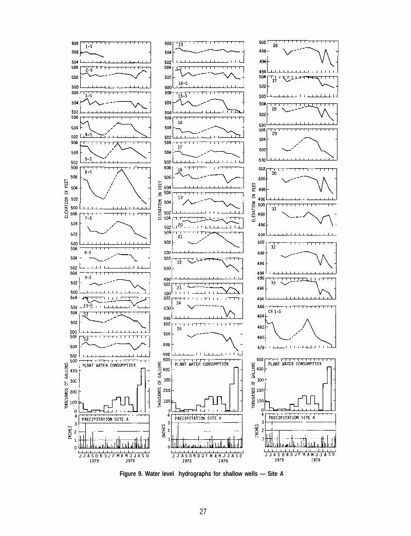
Figure 9. Water level hydrographs for shallow wells — Site A
27
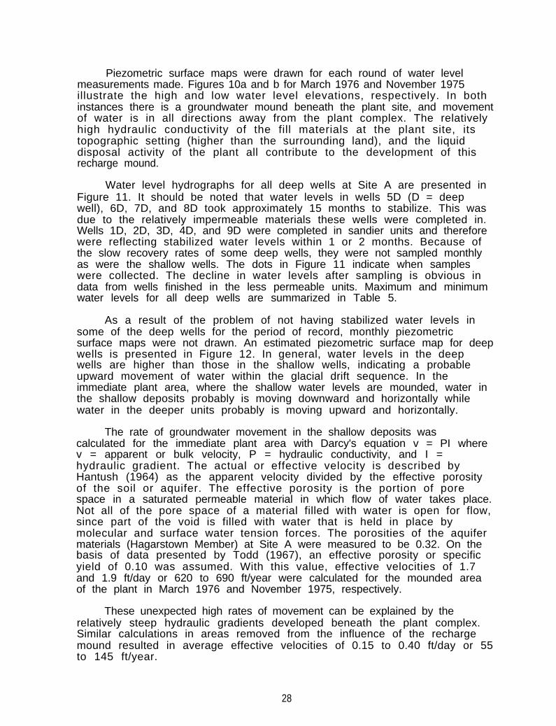
Piezometric surface maps were drawn for each round of water levelmeasurements made. Figures 10a and b for March 1976 and November 1975illustrate the high and low water level elevations, respectively. In bothinstances there is a groundwater mound beneath the plant site, and movementof water is in all directions away from the plant complex. The relativelyhigh hydraulic conductivity of the fill materials at the plant site, itstopographic setting (higher than the surrounding land), and the liquiddisposal activity of the plant all contribute to the development of thisrecharge mound.
Water level hydrographs for all deep wells at Site A are presented inFigure 11. It should be noted that water levels in wells 5D (D = deepwell), 6D, 7D, and 8D took approximately 15 months to stabilize. This wasdue to the relatively impermeable materials these wells were completed in.Wells 1D, 2D, 3D, 4D, and 9D were completed in sandier units and thereforewere reflecting stabilized water levels within 1 or 2 months. Because ofthe slow recovery rates of some deep wells, they were not sampled monthlyas were the shallow wells. The dots in Figure 11 indicate when sampleswere collected. The decline in water levels after sampling is obvious indata from wells finished in the less permeable units. Maximum and minimumwater levels for all deep wells are summarized in Table 5.
As a result of the problem of not having stabilized water levels insome of the deep wells for the period of record, monthly piezometricsurface maps were not drawn. An estimated piezometric surface map for deepwells is presented in Figure 12. In general, water levels in the deepwells are higher than those in the shallow wells, indicating a probableupward movement of water within the glacial drift sequence. In theimmediate plant area, where the shallow water levels are mounded, water inthe shallow deposits probably is moving downward and horizontally whilewater in the deeper units probably is moving upward and horizontally.
The rate of groundwater movement in the shallow deposits wascalculated for the immediate plant area with Darcy's equation v = PI wherev = apparent or bulk velocity, P = hydraulic conductivity, and I =hydraulic gradient. The actual or effective velocity is described byHantush (1964) as the apparent velocity divided by the effective porosityof the soil or aquifer. The effective porosity is the portion of porespace in a saturated permeable material in which flow of water takes place.Not all of the pore space of a material filled with water is open for flow,since part of the void is filled with water that is held in place bymolecular and surface water tension forces. The porosities of the aquifermaterials (Hagarstown Member) at Site A were measured to be 0.32. On thebasis of data presented by Todd (1967), an effective porosity or specificyield of 0.10 was assumed. With this value, effective velocities of 1.7and 1.9 ft/day or 620 to 690 ft/year were calculated for the mounded areaof the plant in March 1976 and November 1975, respectively.
These unexpected high rates of movement can be explained by therelatively steep hydraulic gradients developed beneath the plant complex.Similar calculations in areas removed from the influence of the rechargemound resulted in average effective velocities of 0.15 to 0.40 ft/day or 55to 145 ft/year.
28
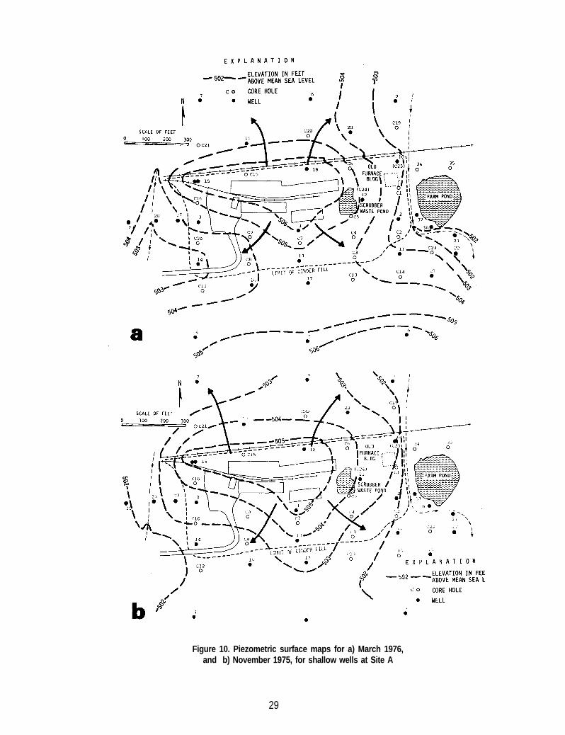
Figure 10. Piezometric surface maps for a) March 1976,and b) November 1975, for shallow wells at Site A
29
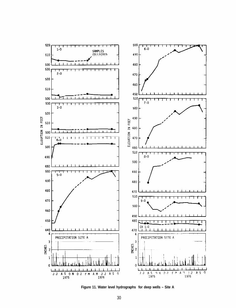
Figure 11. Water level hydrographs for deep wells – Site A
30
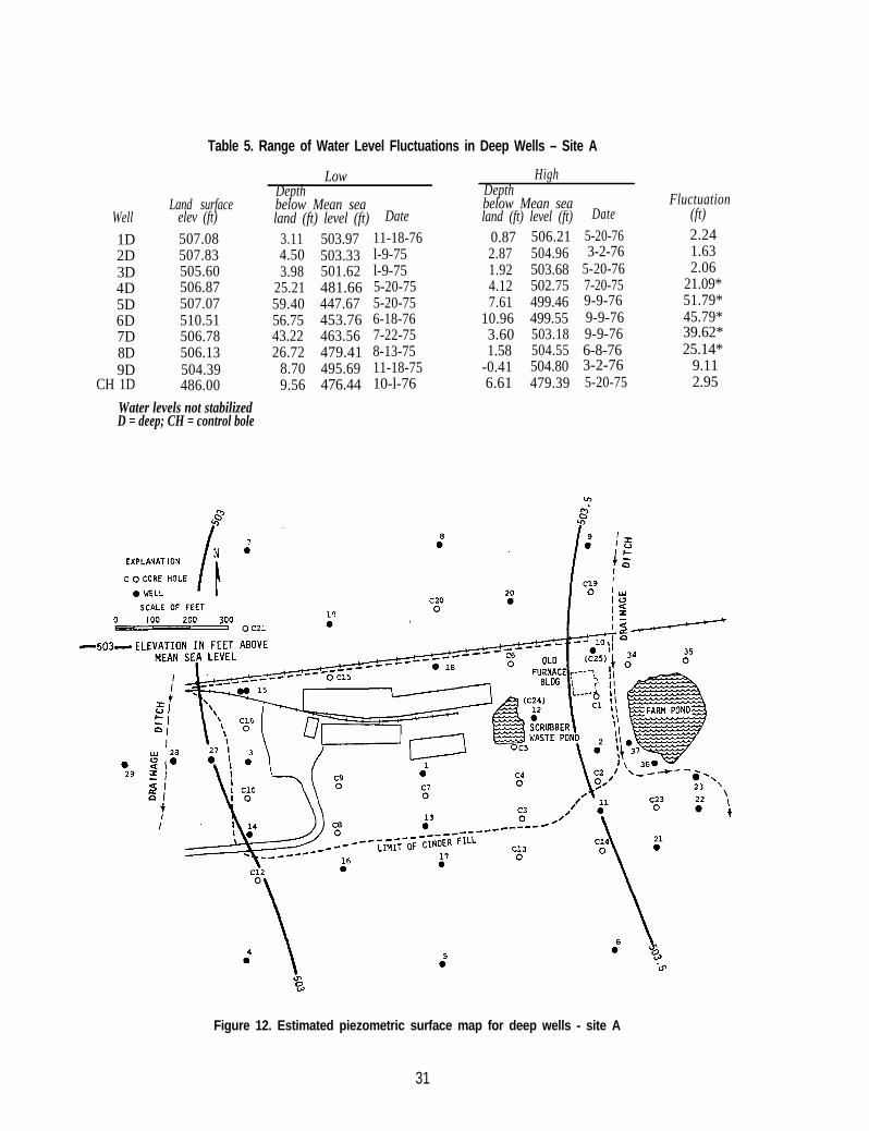
Table 5. Range of Water Level Fluctuations in Deep Wells – Site A
Well
1D2D3D4D5D6D7D8D9D
CH 1D
Land surfaceelev (ft)
507.08507.83505.60506.87507.07510.51506.78506.13504.39486.00
LowDepthbelow Mean sealand (ft) level (ft) Date
3.11 503.97 11-18-76 0.87 506.21 5-20-76 2.244.50 503.33 l-9-75 2.87 504.96 3-2-76 1.633.98 501.62 l-9-75 1.92 503.68 5-20-76 2.06
25.21 481.66 5-20-75 4.12 502.75 7-20-75 21.09*59.40 447.67 5-20-75 7.61 499.46 9-9-76 51.79*56.75 453.76 6-18-76 10.96 499.55 9-9-76 45.79*43.22 463.56 7-22-75 3.60 503.18 9-9-76 39.62*26.72 479.41 8-13-75 1.58 504.55 6-8-76 25.14*
8.70 495.69 11-18-75 -0.41 504.80 3-2-76 9.119.56 476.44 10-l-76 6.61 479.39 5-20-75 2.95
Water levels not stabilizedD = deep; CH = control bole
HighDepthbelow Mean sealand (ft) level (ft) Date
Fluctuation(ft)
Figure 12. Estimated piezometric surface map for deep wells - site A
31
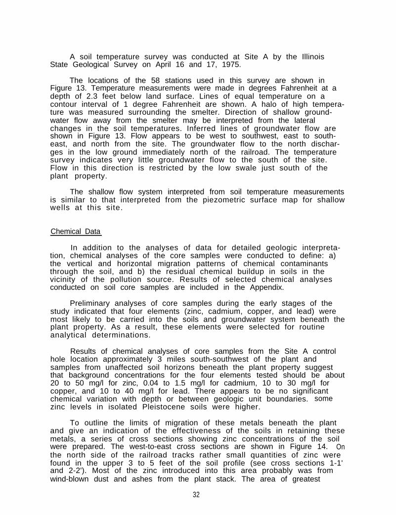
A soil temperature survey was conducted at Site A by the IllinoisState Geological Survey on April 16 and 17, 1975.
The locations of the 58 stations used in this survey are shown inFigure 13. Temperature measurements were made in degrees Fahrenheit at adepth of 2.3 feet below land surface. Lines of equal temperature on acontour interval of 1 degree Fahrenheit are shown. A halo of high tempera-ture was measured surrounding the smelter. Direction of shallow ground-water flow away from the smelter may be interpreted from the lateralchanges in the soil temperatures. Inferred lines of groundwater flow areshown in Figure 13. Flow appears to be west to southwest, east to south-east, and north from the site. The groundwater flow to the north dischar-ges in the low ground immediately north of the railroad. The temperaturesurvey indicates very little groundwater flow to the south of the site.Flow in this direction is restricted by the low swale just south of theplant property.
The shallow flow system interpreted from soil temperature measurementsis similar to that interpreted from the piezometric surface map for shallowwells at this site.
Chemical Data
In addition to the analyses of data for detailed geologic interpreta-tion, chemical analyses of the core samples were conducted to define: a)the vertical and horizontal migration patterns of chemical contaminantsthrough the soil, and b) the residual chemical buildup in soils in thevicinity of the pollution source. Results of selected chemical analysesconducted on soil core samples are included in the Appendix.
Preliminary analyses of core samples during the early stages of thestudy indicated that four elements (zinc, cadmium, copper, and lead) weremost likely to be carried into the soils and groundwater system beneath theplant property. As a result, these elements were selected for routineanalytical determinations.
Results of chemical analyses of core samples from the Site A controlhole location approximately 3 miles south-southwest of the plant andsamples from unaffected soil horizons beneath the plant property suggestthat background concentrations for the four elements tested should be about20 to 50 mg/l for zinc, 0.04 to 1.5 mg/l for cadmium, 10 to 30 mg/l forcopper, and 10 to 40 mg/l for lead. There appears to be no significantchemical variation with depth or between geologic unit boundaries. somezinc levels in isolated Pleistocene soils were higher.
To outline the limits of migration of these metals beneath the plantand give an indication of the effectiveness of the soils in retaining thesemetals, a series of cross sections showing zinc concentrations of the soilwere prepared. The west-to-east cross sections are shown in Figure 14. Onthe north side of the railroad tracks rather small quantities of zinc werefound in the upper 3 to 5 feet of the soil profile (see cross sections 1-1'and 2-2'). Most of the zinc introduced into this area probably was fromwind-blown dust and ashes from the plant stack. The area of greatest
32
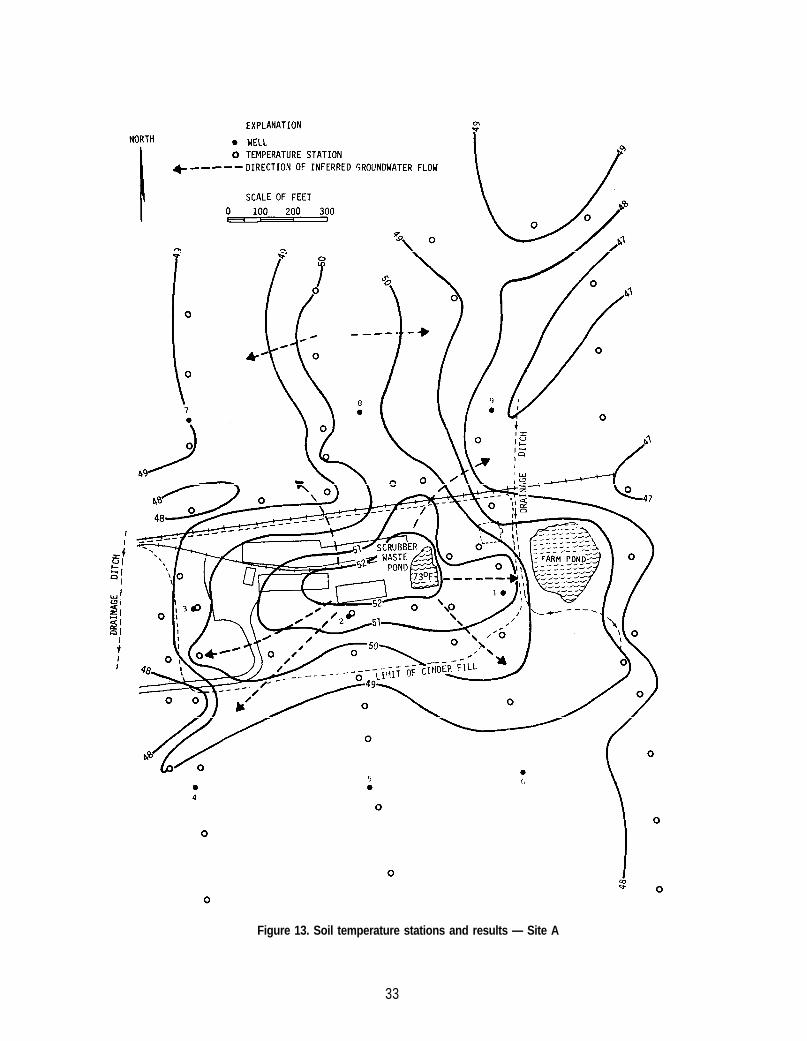
Figure 13. Soil temperature stations and results — Site A
33
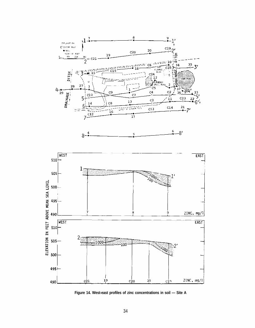
Figure 14. West-east profiles of zinc concentrations in soil — Site A
34
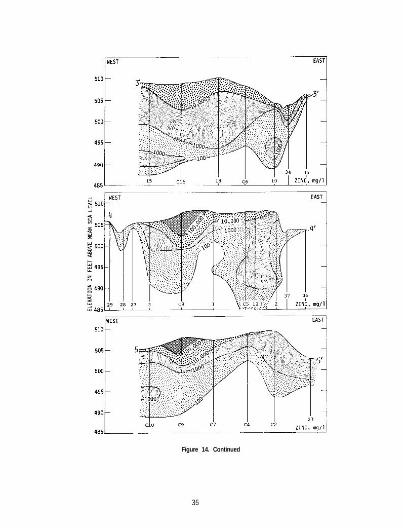
Figure 14. Continued
35
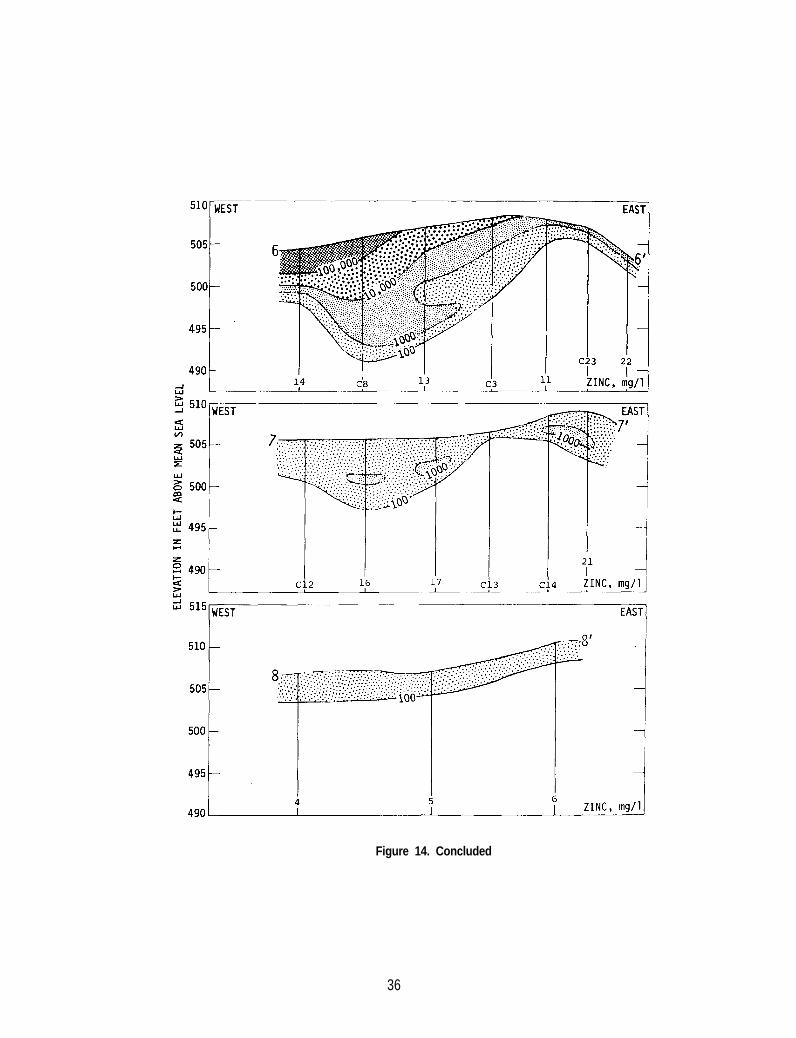
Figure 14. Concluded
36
accumulation and deepest penetration of zinc in the soil occurred immedi-ately beneath the plant property (see cross sections 3-3', 4-4', 5-5', and6-6'). Two principal sources of pollution, the cinders covering the plantproperty and the scrubber wastewater, have resulted in large quantities ofzinc moving into the soil profile. The effect of the scrubber wastewaterdischarge is obvious in cross section 4-4'. Beneath well 12 the depth ofpenetration (to the 100 mg/l boundary) is approximately 28 feet. However,it is interesting to note that lateral migration due to this activity hasstill been very limited. It also is worth noting that no significantlateral migration has taken place beyond the two drainage ditches boundingthe plant on the west and east. Farther south, beyond the limits of thecinder covered portion of the plant property, very limited zinc penetrationhas occurred (see cross sections 7-7' and 8-8').
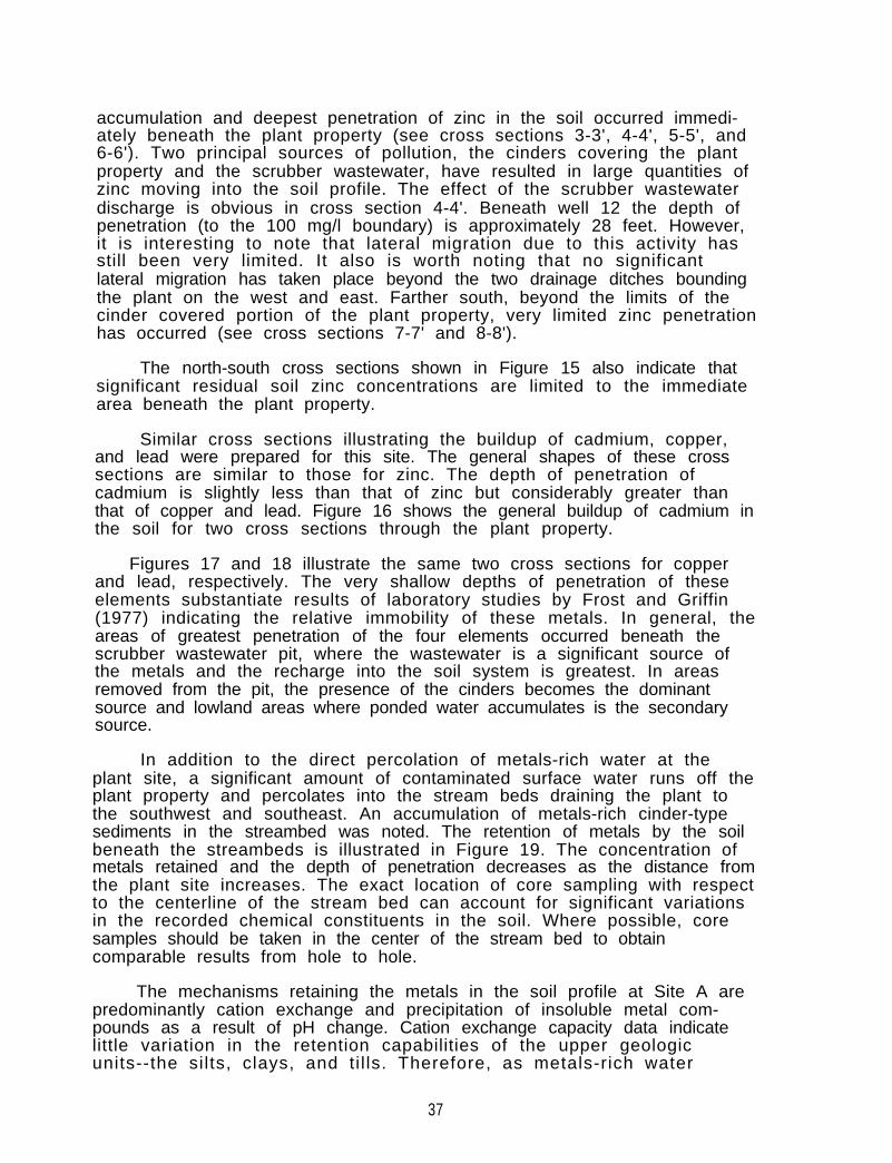
The north-south cross sections shown in Figure 15 also indicate thatsignificant residual soil zinc concentrations are limited to the immediatearea beneath the plant property.
Similar cross sections illustrating the buildup of cadmium, copper,and lead were prepared for this site. The general shapes of these crosssections are similar to those for zinc. The depth of penetration ofcadmium is slightly less than that of zinc but considerably greater thanthat of copper and lead. Figure 16 shows the general buildup of cadmium inthe soil for two cross sections through the plant property.
Figures 17 and 18 illustrate the same two cross sections for copperand lead, respectively. The very shallow depths of penetration of theseelements substantiate results of laboratory studies by Frost and Griffin(1977) indicating the relative immobility of these metals. In general, theareas of greatest penetration of the four elements occurred beneath thescrubber wastewater pit, where the wastewater is a significant source ofthe metals and the recharge into the soil system is greatest. In areasremoved from the pit, the presence of the cinders becomes the dominantsource and lowland areas where ponded water accumulates is the secondarysource.
In addition to the direct percolation of metals-rich water at theplant site, a significant amount of contaminated surface water runs off theplant property and percolates into the stream beds draining the plant tothe southwest and southeast. An accumulation of metals-rich cinder-typesediments in the streambed was noted. The retention of metals by the soilbeneath the streambeds is illustrated in Figure 19. The concentration ofmetals retained and the depth of penetration decreases as the distance fromthe plant site increases. The exact location of core sampling with respectto the centerline of the stream bed can account for significant variationsin the recorded chemical constituents in the soil. Where possible, coresamples should be taken in the center of the stream bed to obtaincomparable results from hole to hole.
The mechanisms retaining the metals in the soil profile at Site A arepredominantly cation exchange and precipitation of insoluble metal com-pounds as a result of pH change. Cation exchange capacity data indicatelittle variation in the retention capabilities of the upper geologicunits--the silts, clays, and ti l ls. Therefore, as metals-rich water
37
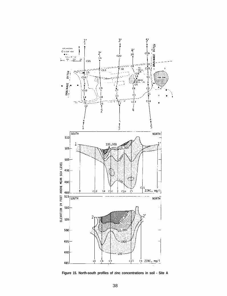
Figure 15. North-south profiles of zinc concentrations in soil - Site A
38
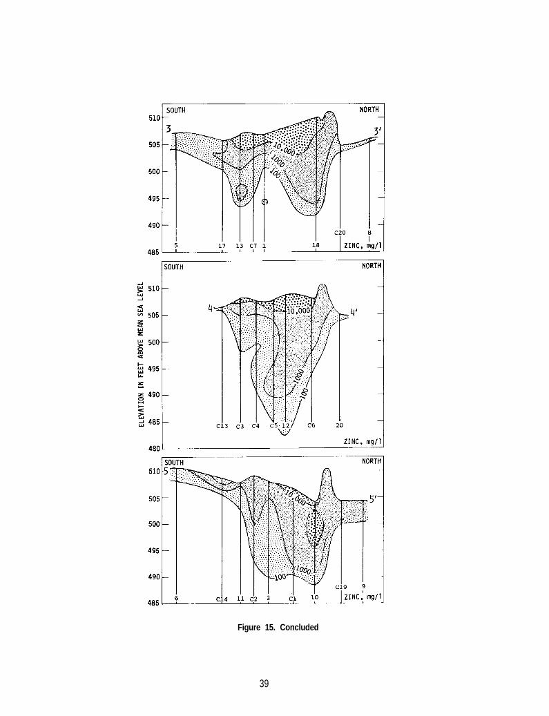
Figure 15. Concluded
39
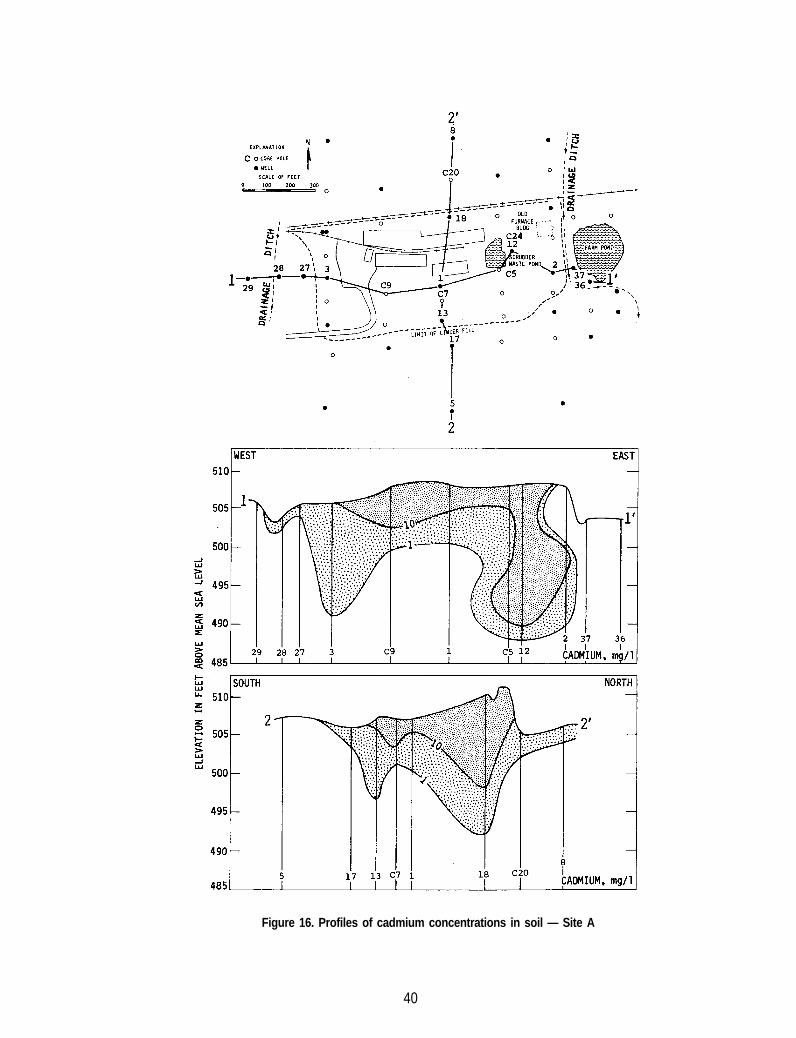
Figure 16. Profiles of cadmium concentrations in soil — Site A
40
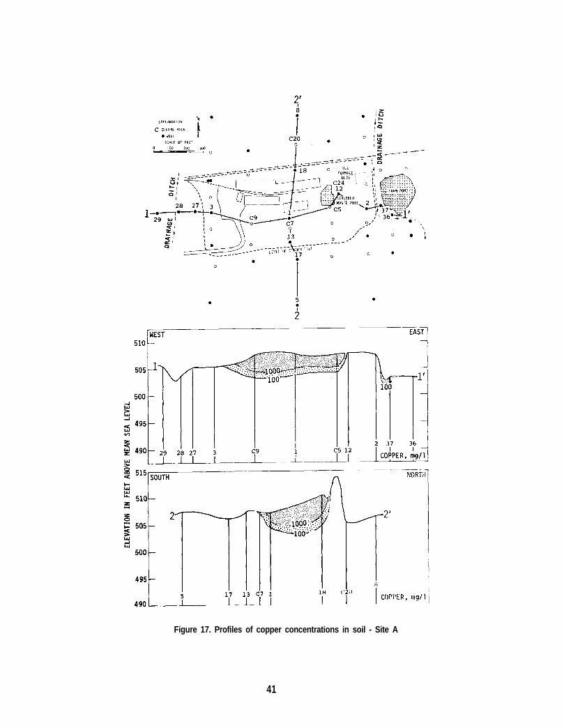
Figure 17. Profiles of copper concentrations in soil - Site A
41
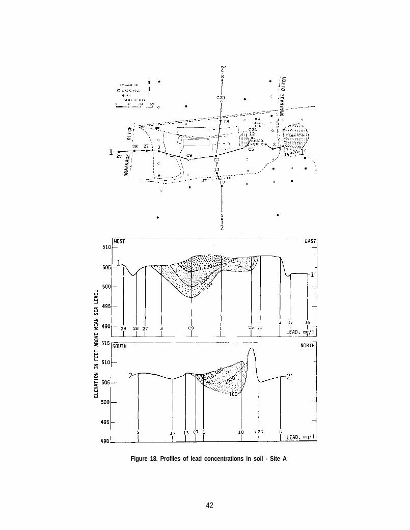
Figure 18. Profiles of lead concentrations in soil - Site A
42
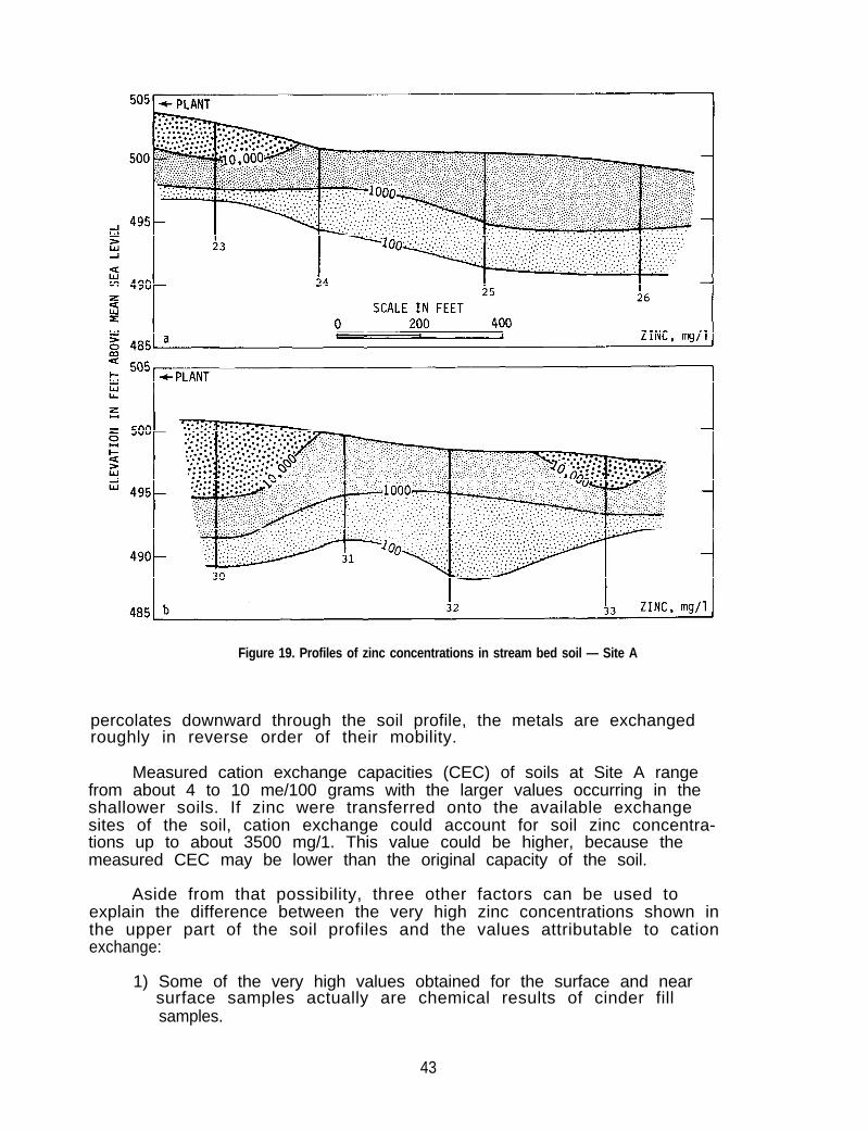
Figure 19. Profiles of zinc concentrations in stream bed soil — Site A
percolates downward through the soil profile, the metals are exchangedroughly in reverse order of their mobility.
Measured cation exchange capacities (CEC) of soils at Site A rangefrom about 4 to 10 me/100 grams with the larger values occurring in theshallower soils. If zinc were transferred onto the available exchangesites of the soil, cation exchange could account for soil zinc concentra-tions up to about 3500 mg/1. This value could be higher, because themeasured CEC may be lower than the original capacity of the soil.
Aside from that possibility, three other factors can be used toexplain the difference between the very high zinc concentrations shown inthe upper part of the soil profiles and the values attributable to cationexchange:
1) Some of the very high values obtained for the surface and nearsurface samples actually are chemical results of cinder fillsamples.
43
2) Immediately beneath the cinder fill, fine-grained sediments fromthe cinders have been illuviated into the underlying soil, alsoresulting in high zinc values of those samples.
3) Soluble and insoluble salts of zinc and other metals may betemporarily stored in the aerated zone during dry periods, waitingfor eventual migration downward with later recharge events.
As the cation exchange capacity of the soil is exhausted and suffi-cient depth is reached to eliminate the three factors just noted, themetals buildup in the soil slowly continues to advance deeper into the soilprofile. As this process occurs, calcium and magnesium are released intothe water from the soil, and the pH of the soil is lowered. When a depthis reached where the soil has not been leached, the pH increases, resultingin the formation of zinc precipitates and a sharp break or decrease in soilzinc content. At Site A, the alteration of soil pH in the upper geologicunits was enhanced by the character of the infiltrating fluid. Samples ofwater collected after percolating through the cinder fill materials formingthe sides of the disposal pit had measured pH values near 5. It can beassumed that the same pH was experienced by water filtering downwardthrough the cinder fill covering the plant surface. It is possible thatsulfur in the cinders was being oxidized and dissolved to form sulfuricacid, thus creating the low pH and increasing the mobility of the zinc.
The conclusions drawn from this field study with regard to the mecha-nism of zinc and other metals fixation are in agreement with the results oflaboratory studies by Frost and Griffin (1977). They conclude thatincreased removal of metals from solution occurs "with increasing pH valuesand with increasing concentrations of the heavy metal in solution."
Representative adsorption isotherms for zinc, copper, and cadmiumdeveloped by Frost and Griffin (1977) are shown in Figure 20. A markedincrease in adsorption occurred for all three ions as the pH increased.The curves for zinc adsorption show sharp increases in gradient at about250 and 100 mg/l at pH 6.75 and 7.0, respectively. The cadmium curves showsharp increases in gradient at about 40 and 5 mg/l at pH 6.5 and 7.0,respectively. A sharp change in the slope of an adsorption isotherm may beindicat ive of the ini t iat ion of precipi tat ion.
Adsorption isotherms obtained for pure montmorillonite clays at pH5.0, developed by Frost and Griffin (1977), are presented in Figure 21.Curve A illustrates the amount of Cd, Zn, or Cu adsorbed by montmorillonitefrom pure Cd(N03)2, Zn(N03)2, or Cu(NO3)2 solutions that wereadjusted to pH 5.0. Curve B illustrates the data obtained when usinglandfill leachate. Maximum adsorption occurred in the pure solutions,whereas adsorption in the leachate was much lower because of competition byorganics and other metals in solution, and organic complexing of themetals. The field situations discussed in this paper lie somewhere betweenthese extremes, and probably closer to the pure solution than the leachate.In studies by Griffin et al. (1976) montomorillonite adsorbed approximately5 times more metals than other clays under similar conditions. It hasalready been noted that the soils at Site A are montmorillonite-rich.
44
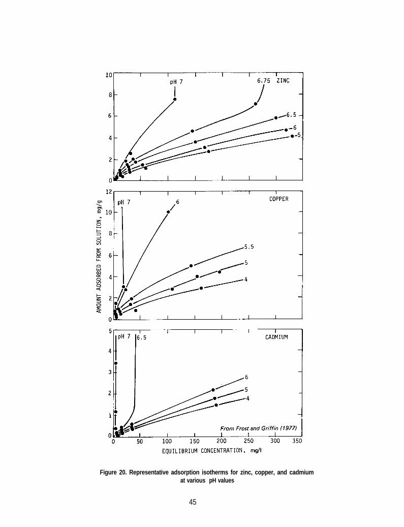
Figure 20. Representative adsorption isotherms for zinc, copper, and cadmiumat various pH values
45
Figure 21. Montmorillonite adsorption isothermsfor cadmium, zinc, and copper
46
The data at Site A indicate that the concentrations of zinc in thesoil are highest in soils with a pH less than 6.5. Soil pH values as lowas 3.4 were recorded and increased with depth to normal values around 7 to8. Therefore, at low pH values, adsorption or cation exchange is themechanism of heavy metal attenuation. The metals are adsorbed by the claysfrom solution as the liquid moves through the subsurface. As the pHincreases, heavy metals not adsorbed by cation exchange are precipitated,thereby reducing concentrations of heavy metals in solution. Thus, pHcontrols the maximum concentration possible in solutions.
Zinc concentrations in water samples collected from wells at Site Aare presented in Table 6. All wells finished at the bedrock surface (1Dthrough 9D) produced water containing less than 0.5 mg/l Zn. The fewisolated samples indicating higher zinc contents were determined not to berepresentat ive.
The zinc content of water collected from the shallow wells tapping theHagarstown sand unit is shown in Figure 22. Figure 22b, illustrating datafor samples collected August 13, 1975, represents the minimum extent ofshallow groundwater contamination, and Figure 22a, illustrating data forsamples collected September 9, 1976, represents the maximum extent ofcontamination. Because the sampling procedure was not satisfactory and theattempt to detect well seal failures was unsuccessful, further analysis ofthe water quality data generated probably is not worthwhile. The samplingprocedure used in this study would account for as much as 45 to 80 percentof the fluctuations noted between sampling periods.
To better define the quality of water in an affected and unaffectedarea, water samples were collected from wells 3S and 6S for total mineralanalysis. The results of these analyses and the analysis of a water samplefrom the shallow control hole well indicate general agreement for 6S (theunaffected area well) and Control Hole 1S. Increases in mineral constitu-ents in the affected area well (3S) are obvious (see Table 7).
Data from well 3S were as expected and substantiate the solubilityproduct calculations. The zinc concentration (750 mg/l) and pH (6.5) arein excellent agreement with the solubility of zinc hydroxide (800 gm/l at6.5 pH).
These conclusions are borne out by the data from the soil cores aswell as the water quality data. For example, the zinc concentration inpiezometer 535 is 750 mg/l, approximately the solubility of zinc hydroxidecalculated at pH 6.5.
Evidence of ion exchange also is shown by the high concentrations ofcalcium (2400 mg/l) and magnesium (893 mg/l) present in this sample (3S).The cation exchange positions in soils in this region of Illinois areprincipally filled with calcium and lesser amounts of magnesium. Grim(1953) indicates that zinc is higher in the montmorillonite exchange seriesthan calcium and magnesium, and thus will replace these ions on the claystructure. According to Griffin et al. (1976), this process releasescalcium and magnesium to the environment even when these are not part ofthe original waste stream.
47
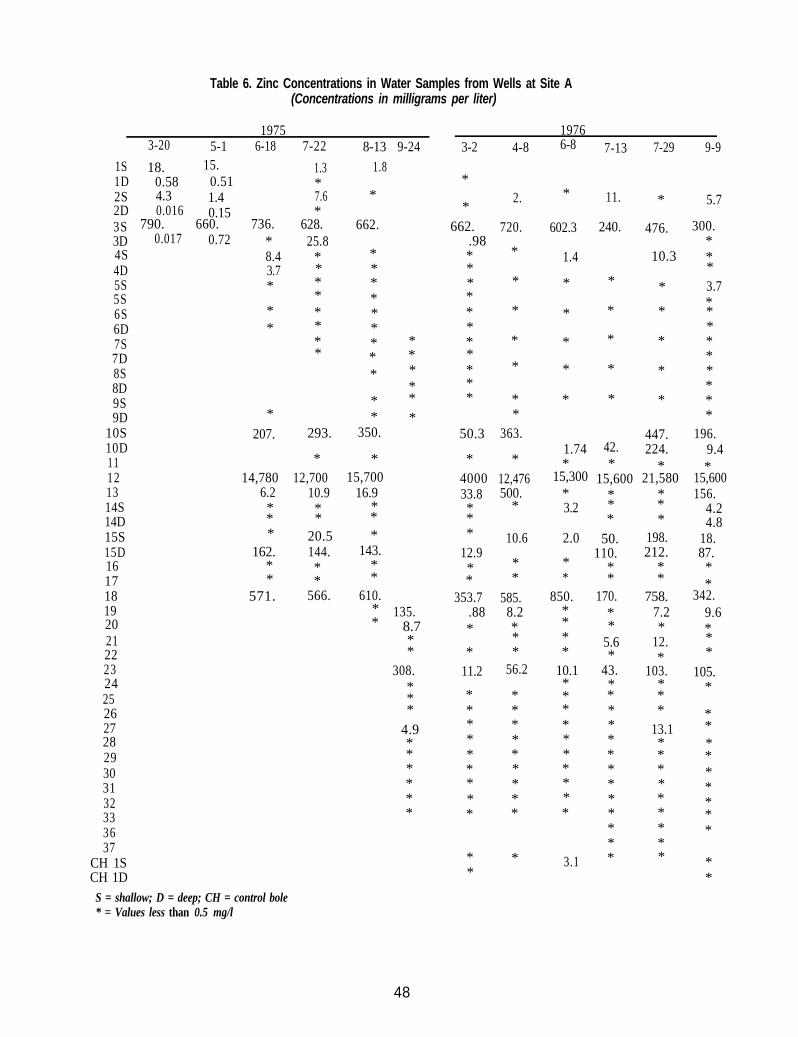
Table 6. Zinc Concentrations in Water Samples from Wells at Site A(Concentrations in milligrams per liter)
1975 19763-20 5-1 6-18 7-22 8-13 9-24 3-2 4-8 6-8 7-13 7-29 9-9
1S 18. 15. 1.3 1.81D 0.58 0.51 *2S 4.3 1.4 7.6 *2D 0.016 0.15 *3S 790. 660. 736. 628. 662.3D 0.017 0.72 * 25.84S 8.4 * *4D 3.7 * * *5S * * *5S * *6S * * *6D * * *7S * *7D * *8S *8D9S *9D * *
10S 207. 293. 350.10D11 * *12 14,780 12,700 15,700 21,58013 6.2 10.9 16.914S * * * * *14D * * *
15S * 20.5 *15D 162. 144. 143.16 * * *17 * * * * *18 571. 566. 610. 342.19 *20 * *21 *22 *23 103.24 *25 *26272829 *303132333637
CH 1SCH 1D
*
*662.
.98***********
50.3
*400033.8***
12.9**
353.7.88*
*11.2
*********
**
******
135.8.7**
308.***
4.9******
*
105.*
*********
**
S = shallow; D = deep; CH = control bole* = Values less than 0.5 mg/l
2.
*
*
*
*
*
**
363.
*12,476500.
*
10.6
**
585.8.2***
56.2
*********
*
720.
* 5.7
476. 300.*
10.3 *
* 3.7*
* **
* **
* **
* **
447. 196.224. 9.4
* *
*
*50.
110.*
170.**
5.6
43.*************
*
*198.212.
*
758.7.2*
12.*
*
*13.1*
*******
156.4.24.8
18.87.*
9.6*
*
48
* 11.
602.3 240.
1.4
* *
* *
* *
* *
* *
1.74 42.* *
15,300 15,600 15,600*3.2
2.0
**
850.*
**
10.1
*********
3.1
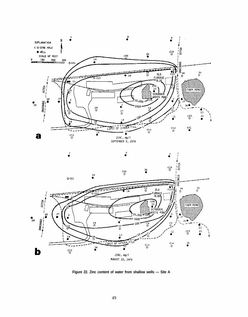
Figure 22. Zinc content of water from shallow wells — Site A
49
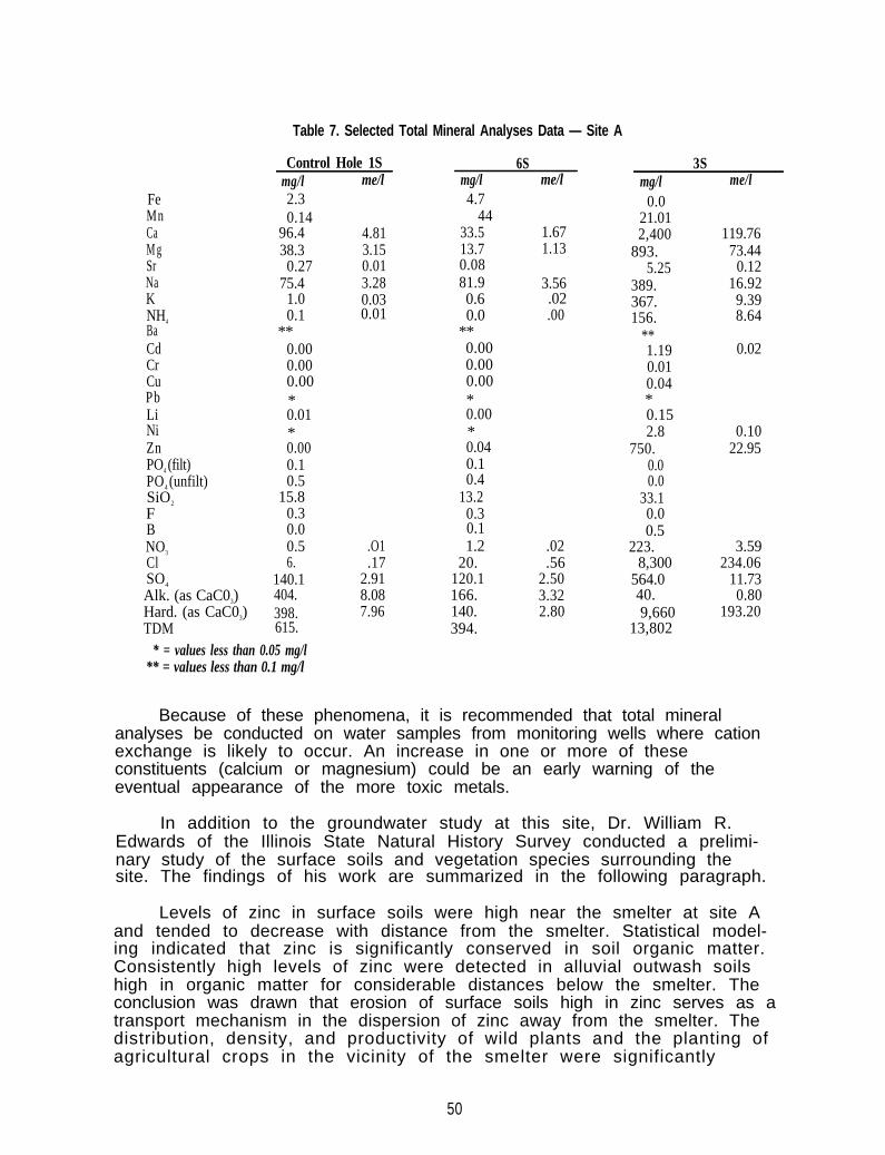
Table 7. Selected Total Mineral Analyses Data — Site A
Control Hole 1S 6S 3Smg/l
Fe 2.3Mn 0.14Ca 96.4M g 38.3Sr 0.27Na 75.4K 1.0NH4 0.1Ba **Cd 0.00Cr 0.00Cu 0.00Pb *Li 0.01Ni *Zn 0.00PO4 (filt) 0.1PO4 (unfilt) 0.5SiO2 15.8F 0.3B 0.0NO3 0.5Cl 6.SO4 140.1Alk. (as CaC03) 404.Hard. (as CaC03) 398.TDM 615.
* = values less than 0.05 mg/l** = values less than 0.1 mg/l
me/l
4.813.150.013.280.030.01
.O1
.172.918.087.96
mg/l4.7
4433.513.70.0881.90.60.0
**0.000.000.00*0.00*0.040.10.4
13.20.30.11.2
20.120.1166.140.394.
me/l
1.671.13
3.56.02.00
.02
.562.503.322.80
mg/l0.0
21.012,400
893.5.25
389.367.156.
**1.190.010.04*0.152.8
750.0.00.0
33.10.00.5
223.8,300
564.040.9,660
13,802
me/l
119.7673.44
0.1216.92
9.398.64
0.02
0.1022.95
3.59234.06
11.730.80
193.20
Because of these phenomena, it is recommended that total mineralanalyses be conducted on water samples from monitoring wells where cationexchange is likely to occur. An increase in one or more of theseconstituents (calcium or magnesium) could be an early warning of theeventual appearance of the more toxic metals.
In addition to the groundwater study at this site, Dr. William R.Edwards of the Illinois State Natural History Survey conducted a prelimi-nary study of the surface soils and vegetation species surrounding thesite. The findings of his work are summarized in the following paragraph.
Levels of zinc in surface soils were high near the smelter at site Aand tended to decrease with distance from the smelter. Statistical model-ing indicated that zinc is significantly conserved in soil organic matter.Consistently high levels of zinc were detected in alluvial outwash soilshigh in organic matter for considerable distances below the smelter. Theconclusion was drawn that erosion of surface soils high in zinc serves as atransport mechanism in the dispersion of zinc away from the smelter. Thedistribution, density, and productivity of wild plants and the planting ofagricultural crops in the vicinity of the smelter were significantly
50
related to the zinc content of surface soils. Chemical analyses of plantsindicated: a) that the zinc status of plants reflects, at least in part,the zinc status of their environments; b) that different plants, even thosegrowing in close association, evidence quite different levels of zinc; andc) that different parts of plants concentrate zinc at different rates.Although statistical analyses have not been completed, all observationsthat bear on findings of previously reported research on zinc plantrelationships are in general agreement with the earlier findings. Thehypothesis is advanced that amino acids may be involved in the transportand accumulation of zinc in plants, and are related to the concentration ofzinc in the soil solution and soil organic matter.
The soil coring and sampling of wells at Site A defined the migrationpatterns of toxic metals from this site into the ground and shallow ground-water system. Cation exchange and precipitation of metal compounds as aresult of the change in pH of the infiltrating fluid are the principalattenuating mechanisms influencing the metals movement. The geologicsetting has the ability to contain high concentrations of toxic metals overan extended length of time.
Site B
Site B also is a secondary zinc smelter located in south-centralIllinois. As at Site A, this was a primary smelting operation processingzinc ore from about 1904 until 1962. It was then converted to a secondarysmelting operation and currently is reprocessing selected scrap metals.Wastes from this smelter during the early years of operation were the sametype of metals-rich ashes and cinders as at Site A. An area of approxi-mately 38 acres at the plant site is covered with from 1 to 15 feet ofthese metals-rich cinders.
In compliance with air pollution regulations, this industry installedan electric precipitator on its stacks in 1968. The precipitated particlesare immediately recycled into the smelting process.
The suspected sources for groundwater contamination at this site wereessentially the cinder fill material and stored scrap or junk on the plantproperty. Since this site is so similar to Site A, a minimum amount oftime and effort were spent in studying it. A basic grid of 9 locations (22wells) was established to form a basis for study (Figure 23). An addi-tional six wells eventually were constructed to permit more detailed metalsmigration definition. Total well and coring footages are about 1010 and785 feet, respectively.
Geology
The glacial drift at this site ranges in thickness from 40 to 65 feet,becoming thicker where the drift fills a northwest-southeast trendingbedrock valley (Figure 24a and b). The elevation of the Pennsylvanianbedrock ranges from greater than 410 feet above sea level in the southwestand northeast portions of the site to less than 390 feet in the valley tothe northwest. The stratigraphic units are continuous across the site and
51
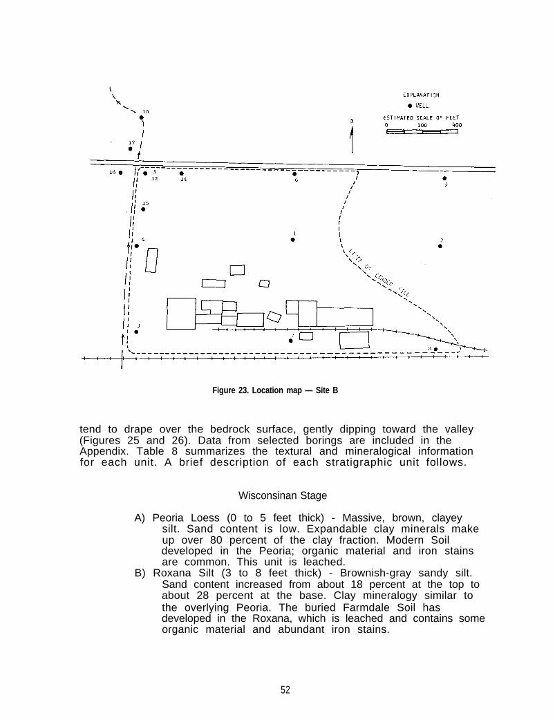
Figure 23. Location map — Site B
tend to drape over the bedrock surface, gently dipping toward the valley(Figures 25 and 26). Data from selected borings are included in theAppendix. Table 8 summarizes the textural and mineralogical informationfor each unit. A brief description of each stratigraphic unit follows.
Wisconsinan Stage
A) Peoria Loess (0 to 5 feet thick) - Massive, brown, clayeysilt. Sand content is low. Expandable clay minerals makeup over 80 percent of the clay fraction. Modern Soildeveloped in the Peoria; organic material and iron stainsare common. This unit is leached.
B) Roxana Silt (3 to 8 feet thick) - Brownish-gray sandy silt.Sand content increased from about 18 percent at the top toabout 28 percent at the base. Clay mineralogy similar tothe overlying Peoria. The buried Farmdale Soil hasdeveloped in the Roxana, which is leached and contains someorganic material and abundant iron stains.
52
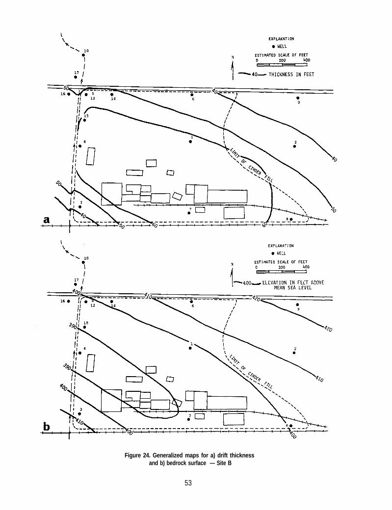
Figure 24. Generalized maps for a) drift thicknessand b) bedrock surface — Site B
53
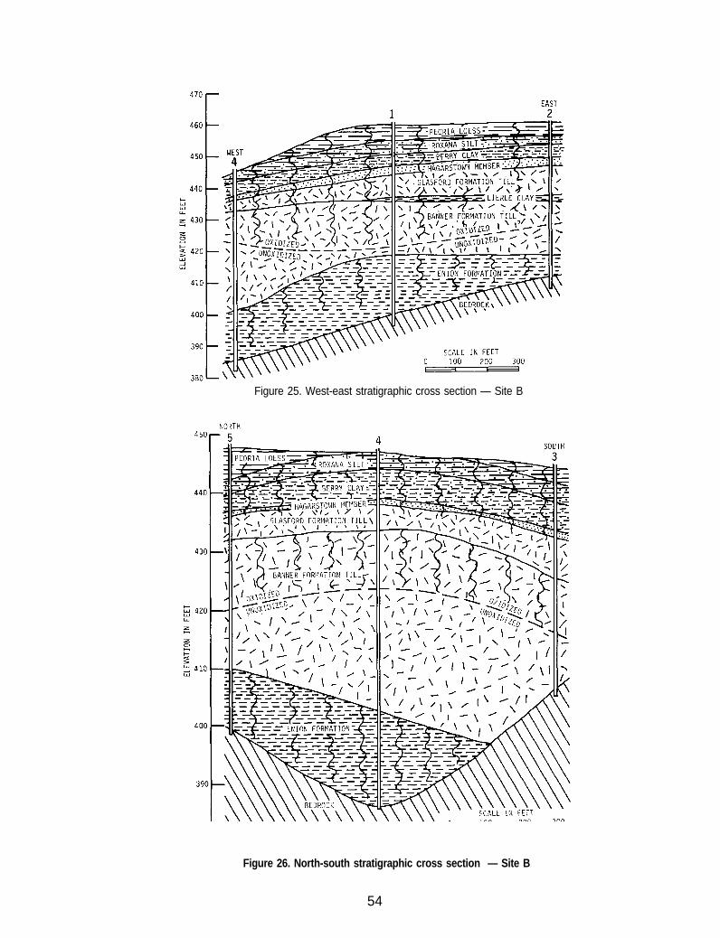
Figure 25. West-east stratigraphic cross section — Site B
Figure 26. North-south stratigraphic cross section — Site B
54
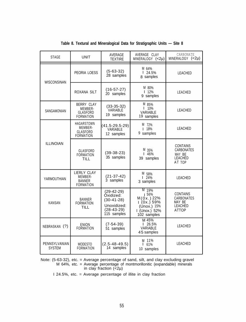
Table 8. Textural and Mineralogical Data for Stratigraphic Units — Site 8
CARBONATESTAGE
AVERAGE CLAYUNIT
AVERAGETEXTIRE MINERALOGY (<2µ) MINERALOGY (<2µ)
M 64%PEORIA LOESS (5-63-32) I
28 samples24.5% LEACHED
8 samplesWISCONSINAN
M 80%ROXANA SILT
(16-57-27)20 samples I 12% LEACHED
9 samples
BERRY CLAY M 85%MEMBER-
(33-35-32)VARIABLE I
SANGAMONIAN10% LEACHED
GLASFORD VARIABLEFORMATION 19 samples 19 samples
HAGARSTOWN M 72%MEMBER- (41.5-29.5-29)
VARIABLE I 18% LEACHEDGLASFORD
FORMATION 12 samples 9 samples
ILLINOIANCONTAINS
GLASFORD M 35% CARBONATESFORMATION (39-38-23) I 46% MAY BE
TILL 35 samples 39 samples LEACHEDAT TOP
LIERLY CLAY M 58%MEMBER- (21-37-42)
YARMOUTHIAN I 24% LEACHEDBANNER 3 samples 3 samples
FORMATION
(29-42-29) M 19%Oxidized: I 56% CONTAINS
BANNER (30-41-28) M (0x . ) 22% CARBONATESKANSAN FORMATION I (0x.) 59% MAY BE
Unoxidized:TILL (Unox.) 15% LEACHED(28-43-29) I (Unox.) 52%115 samples
ATTOP102 samples
M 45%ENIONNEBRASKAN (?) (7-54-39) I 26.5% LEACHED
FORMATION 51 samples VARIABLE45 samples
M 11%PENNSYLVANIAN MODESTO (2.5-48-49.5) I LEACHED61%
SYSTEM FORMATION 14 samples 10 samples
Note: (5-63-32), etc. = Average percentage of sand, silt, and clay excluding gravelM 64%, etc. = Average percentage of montmorillonitic (expandable) minerals
in clay fraction (<2µ)
I 24.5%, etc. = Average percentage of illite in clay fraction
55
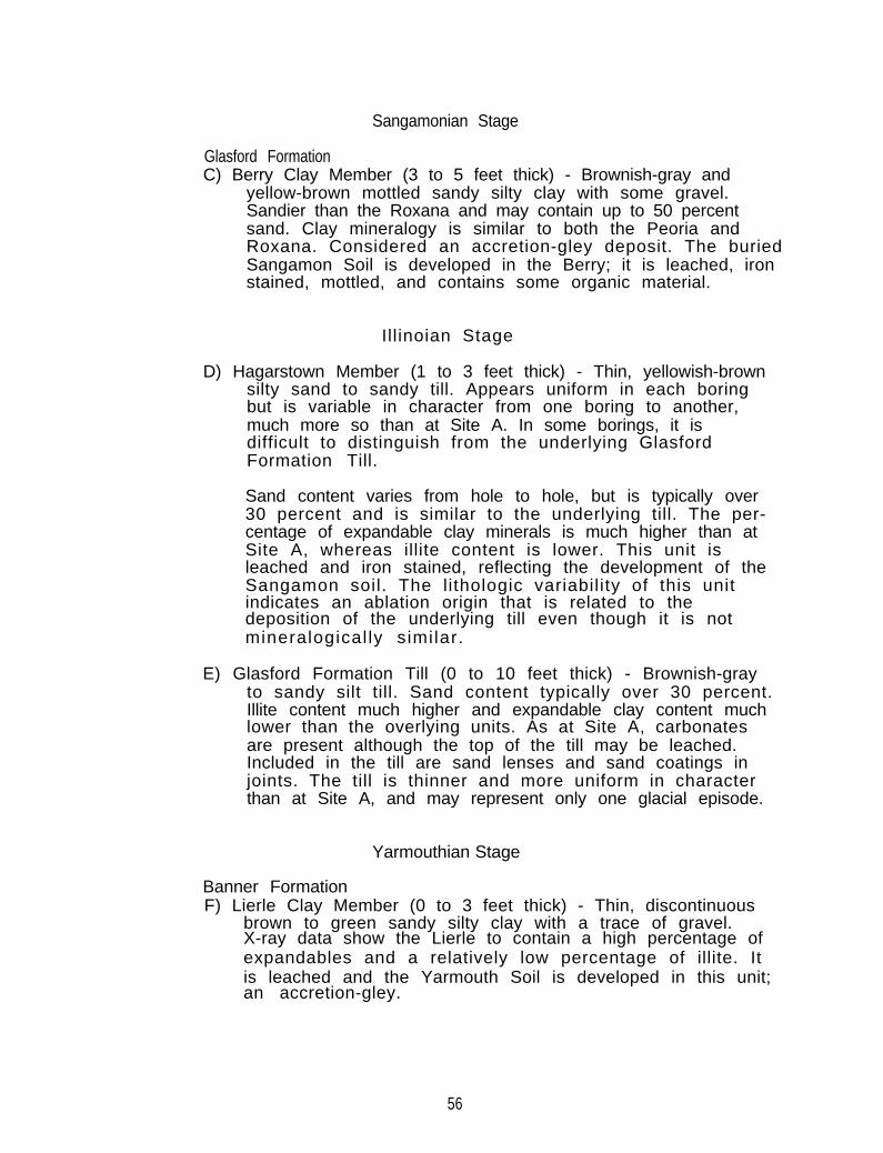
Sangamonian Stage
Glasford FormationC) Berry Clay Member (3 to 5 feet thick) - Brownish-gray and
yellow-brown mottled sandy silty clay with some gravel.Sandier than the Roxana and may contain up to 50 percentsand. Clay mineralogy is similar to both the Peoria andRoxana. Considered an accretion-gley deposit. The buriedSangamon Soil is developed in the Berry; it is leached, ironstained, mottled, and contains some organic material.
Ill inoian Stage
D) Hagarstown Member (1 to 3 feet thick) - Thin, yellowish-brownsilty sand to sandy till. Appears uniform in each boringbut is variable in character from one boring to another,much more so than at Site A. In some borings, it isdifficult to distinguish from the underlying GlasfordFormation Till.
Sand content varies from hole to hole, but is typically over30 percent and is similar to the underlying till. The per-centage of expandable clay minerals is much higher than atSite A, whereas illite content is lower. This unit isleached and iron stained, reflecting the development of theSangamon soil. The lithologic variability of this unitindicates an ablation origin that is related to the deposition of the underlying till even though it is notmineralogical ly similar.
E) Glasford Formation Till (0 to 10 feet thick) - Brownish-grayto sandy silt till. Sand content typically over 30 percent.Illite content much higher and expandable clay content muchlower than the overlying units. As at Site A, carbonatesare present although the top of the till may be leached.Included in the till are sand lenses and sand coatings injoints. The till is thinner and more uniform in characterthan at Site A, and may represent only one glacial episode.
Yarmouthian Stage
Banner FormationF) Lierle Clay Member (0 to 3 feet thick) - Thin, discontinuous
brown to green sandy silty clay with a trace of gravel.X-ray data show the Lierle to contain a high percentage ofexpandables and a relatively low percentage of illite. Itis leached and the Yarmouth Soil is developed in this unit;an accretion-gley.
56
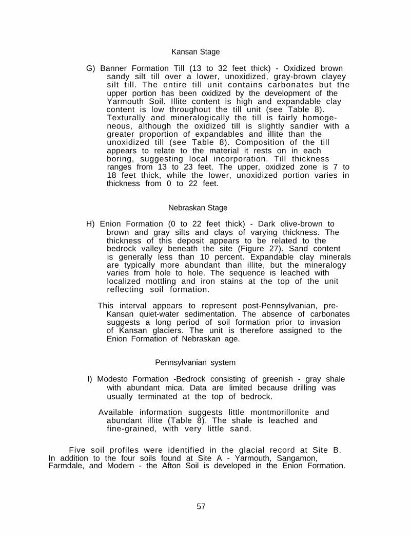
Kansan Stage
G) Banner Formation Till (13 to 32 feet thick) - Oxidized brownsandy silt till over a lower, unoxidized, gray-brown clayeysilt t i l l . The entire ti l l unit contains carbonates but theupper portion has been oxidized by the development of theYarmouth Soil. Illite content is high and expandable claycontent is low throughout the till unit (see Table 8).Texturally and mineralogically the till is fairly homoge-neous, although the oxidized till is slightly sandier with agreater proportion of expandables and illite than theunoxidized till (see Table 8). Composition of the tillappears to relate to the material it rests on in eachboring, suggesting local incorporation. Till thicknessranges from 13 to 23 feet. The upper, oxidized zone is 7 to18 feet thick, while the lower, unoxidized portion varies inthickness from 0 to 22 feet.
Nebraskan Stage
H) Enion Formation (0 to 22 feet thick) - Dark olive-brown tobrown and gray silts and clays of varying thickness. Thethickness of this deposit appears to be related to thebedrock valley beneath the site (Figure 27). Sand contentis generally less than 10 percent. Expandable clay mineralsare typically more abundant than illite, but the mineralogyvaries from hole to hole. The sequence is leached withlocalized mottling and iron stains at the top of the unitreflecting soil formation.
This interval appears to represent post-Pennsylvanian, pre-Kansan quiet-water sedimentation. The absence of carbonatessuggests a long period of soil formation prior to invasionof Kansan glaciers. The unit is therefore assigned to theEnion Formation of Nebraskan age.
Pennsylvanian system
I) Modesto Formation -Bedrock consisting of greenish - gray shale with abundant mica. Data are limited because drilling was usually terminated at the top of bedrock.
Available information suggests little montmorillonite andabundant illite (Table 8). The shale is leached andfine-grained, with very little sand.
Five soil profiles were identified in the glacial record at Site B.In addition to the four soils found at Site A - Yarmouth, Sangamon,Farmdale, and Modern - the Afton Soil is developed in the Enion Formation.
57
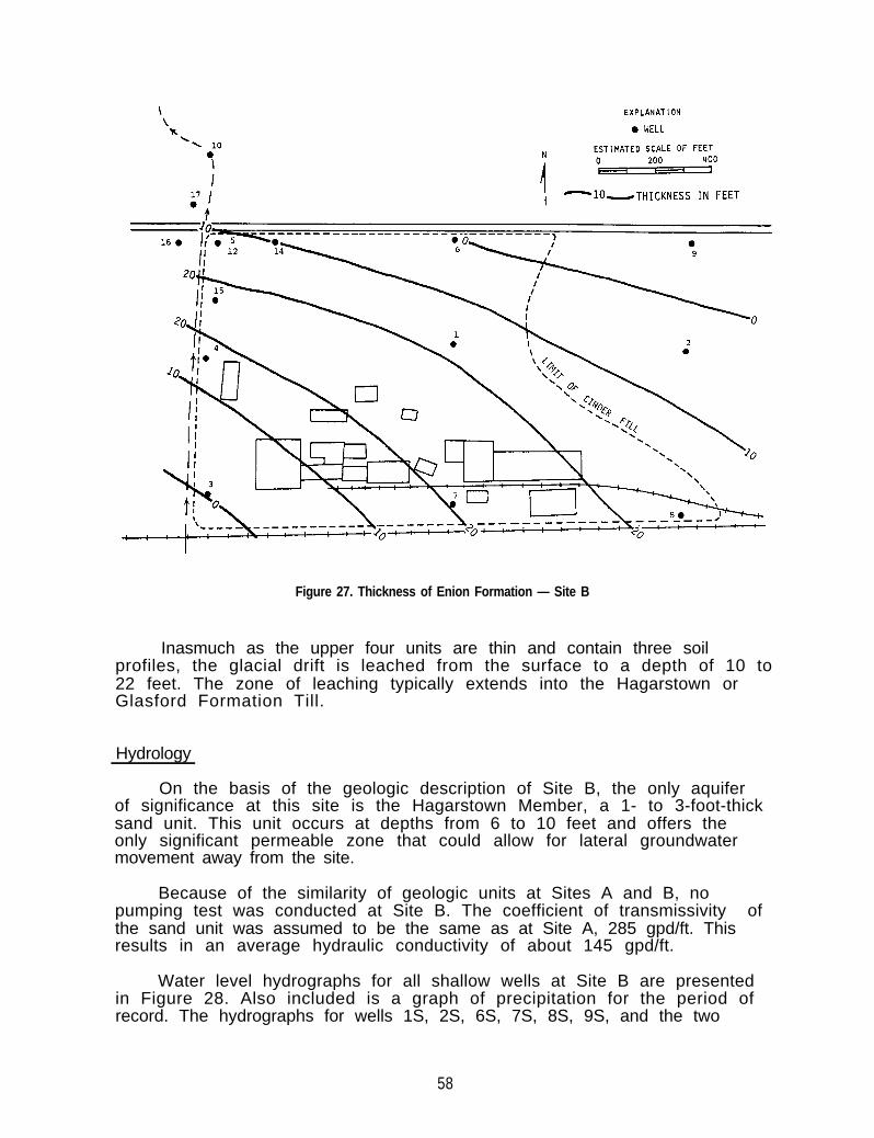
Figure 27. Thickness of Enion Formation — Site B
Inasmuch as the upper four units are thin and contain three soilprofiles, the glacial drift is leached from the surface to a depth of 10 to22 feet. The zone of leaching typically extends into the Hagarstown orGlasford Formation Till.
Hydrology
On the basis of the geologic description of Site B, the only aquiferof significance at this site is the Hagarstown Member, a 1- to 3-foot-thicksand unit. This unit occurs at depths from 6 to 10 feet and offers theonly significant permeable zone that could allow for lateral groundwatermovement away from the site.
Because of the similarity of geologic units at Sites A and B, nopumping test was conducted at Site B. The coefficient of transmissivity ofthe sand unit was assumed to be the same as at Site A, 285 gpd/ft. Thisresults in an average hydraulic conductivity of about 145 gpd/ft.
Water level hydrographs for all shallow wells at Site B are presentedin Figure 28. Also included is a graph of precipitation for the period ofrecord. The hydrographs for wells 1S, 2S, 6S, 7S, 8S, 9S, and the two
58
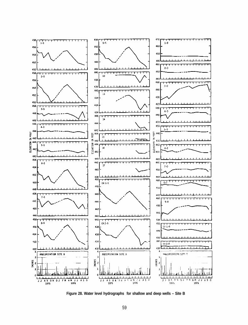
Figure 28. Water level hydrographs for shallow and deep wells – Site B
59
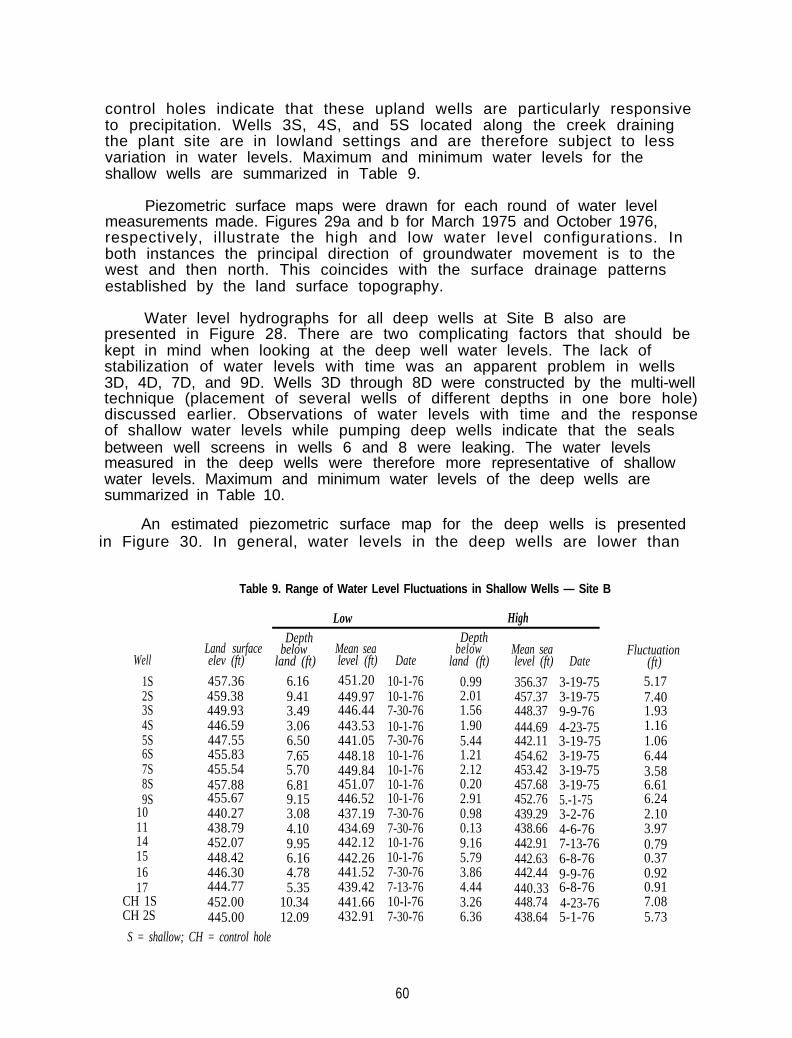
control holes indicate that these upland wells are particularly responsiveto precipitation. Wells 3S, 4S, and 5S located along the creek drainingthe plant site are in lowland settings and are therefore subject to lessvariation in water levels. Maximum and minimum water levels for theshallow wells are summarized in Table 9.
Piezometric surface maps were drawn for each round of water levelmeasurements made. Figures 29a and b for March 1975 and October 1976,respectively, illustrate the high and low water level configurations. Inboth instances the principal direction of groundwater movement is to thewest and then north. This coincides with the surface drainage patternsestablished by the land surface topography.
Water level hydrographs for all deep wells at Site B also arepresented in Figure 28. There are two complicating factors that should bekept in mind when looking at the deep well water levels. The lack ofstabilization of water levels with time was an apparent problem in wells3D, 4D, 7D, and 9D. Wells 3D through 8D were constructed by the multi-welltechnique (placement of several wells of different depths in one bore hole)discussed earlier. Observations of water levels with time and the responseof shallow water levels while pumping deep wells indicate that the sealsbetween well screens in wells 6 and 8 were leaking. The water levelsmeasured in the deep wells were therefore more representative of shallowwater levels. Maximum and minimum water levels of the deep wells aresummarized in Table 10.
An estimated piezometric surface map for the deep wells is presentedin Figure 30. In general, water levels in the deep wells are lower than
Table 9. Range of Water Level Fluctuations in Shallow Wells — Site B
Low HighDepth
Land surface belowWell elev (ft) land (ft)
1S 457.36 6.162S 459.38 9.413S 449.93 3.494S 446.59 3.065S 447.55 6.506S 455.83 7.657S 455.54 5.708S 457.88 6.819S 455.67 9.15
10 440.27 3.0811 438.79 4.1014 452.07 9.9515 448.42 6.1616 446.30 4.7817 444.77 5.35
CH 1S 452.00 10.34CH 2S 445.00 12.09S = shallow; CH = control hole
Mean sealevel (ft) Date
451.20 10-1-76449.97 10-1-76446.44 7-30-76443.53 10-1-76441.05 7-30-76448.18 10-1-76449.84 10-1-76451.07 10-1-76446.52 10-1-76437.19 7-30-76434.69 7-30-76442.12 10-1-76442.26 10-1-76441.52 7-30-76439.42 7-13-76441.66 10-l-76432.91 7-30-76
Depthbelow
land (ft)
0.992.011.561.905.441.212.120.202.910.980.139.165.793.864.443.266.36
Mean sea Fluctuationlevel (ft) Date (ft)
356.37 3-19-75 5.17457.37 3-19-75 7.40448.37 9-9-76 1.93444.69 4-23-75 1.16442.11 3-19-75 1.06454.62 3-19-75 6.44453.42 3-19-75 3.58457.68 3-19-75 6.61452.76 5.-1-75 6.24439.29 3-2-76 2.10438.66 4-6-76 3.97442.91 7-13-76 0.79442.63 6-8-76 0.37442.44 9-9-76 0.92440.33 6-8-76 0.91448.74 4-23-76 7.08438.64 5-1-76 5.73
60
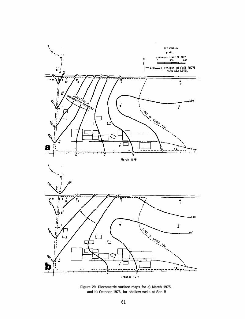
Figure 29. Piezometric surface maps for a) March 1975,and b) October 1976, for shallow wells at Site B
61
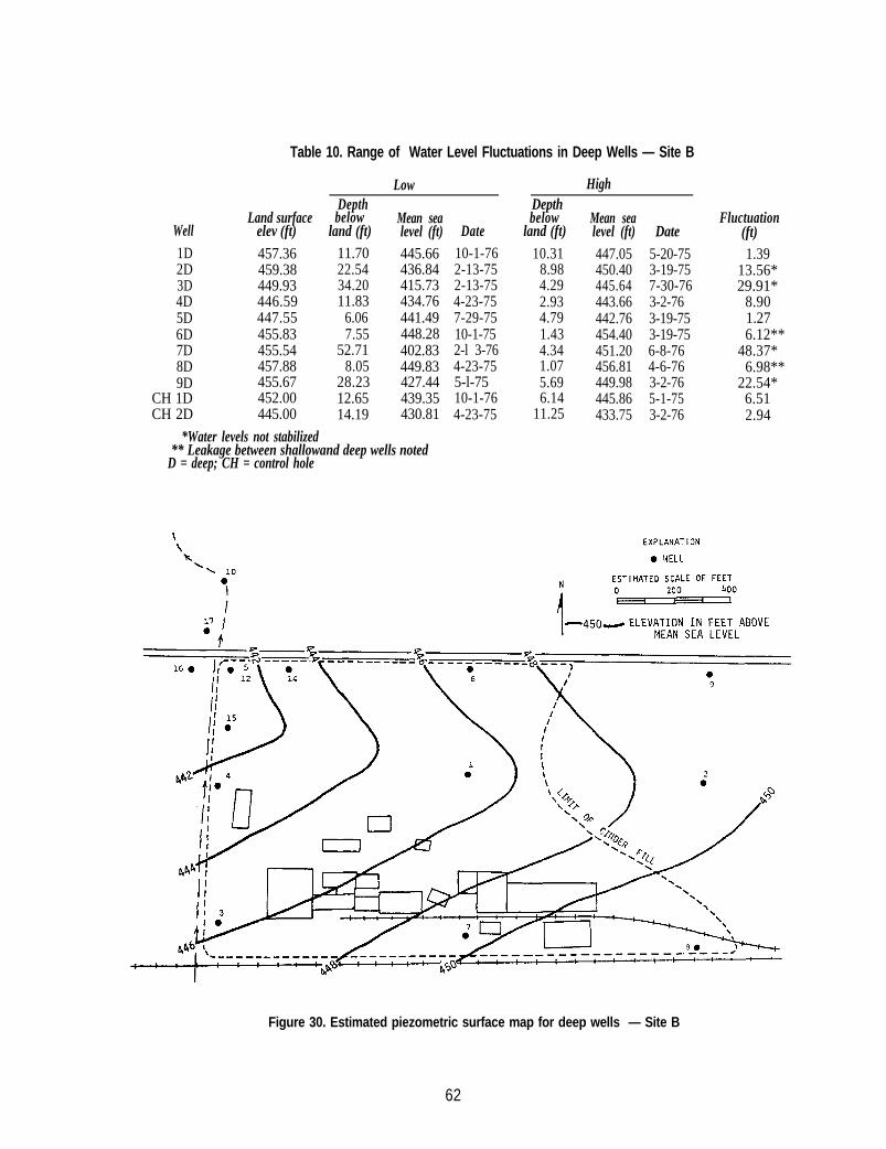
Table 10. Range of Water Level Fluctuations in Deep Wells — Site B
Low
Well
DepthLand surface below Mean sea
elev (ft) land (ft) level (ft) Date1D 457.362D 459.383D 449.934D 446.595D 447.556D 455.837D 455.548D 457.889D 455.67
CH 1D 452.00CH 2D 445.00
11.70 445.66 10-1-7622.54 436.84 2-13-7534.20 415.73 2-13-7511.83 434.76 4-23-75
6.06 441.49 7-29-757.55 448.28 10-1-75
52.71 402.83 2-l 3-768.05 449.83 4-23-75
28.23 427.44 5-l-7512.65 439.35 10-1-7614.19 430.81 4-23-75
Depthbelow
land (ft)
10.318.984.292.934.791.434.341.075.696.14
11.25
High
Mean sea Fluctuationlevel (ft) Date (ft)447.05 5-20-75 1.39450.40 3-19-75 13.56*445.64 7-30-76 29.91*443.66 3-2-76 8.90442.76 3-19-75 1.27454.40 3-19-75 6.12**451.20 6-8-76 48.37*456.81 4-6-76 6.98**449.98 3-2-76 22.54*445.86 5-1-75 6.51433.75 3-2-76 2.94
*Water levels not stabilized** Leakage between shallowand deep wells noted
D = deep; CH = control hole
Figure 30. Estimated piezometric surface map for deep wells — Site B
62
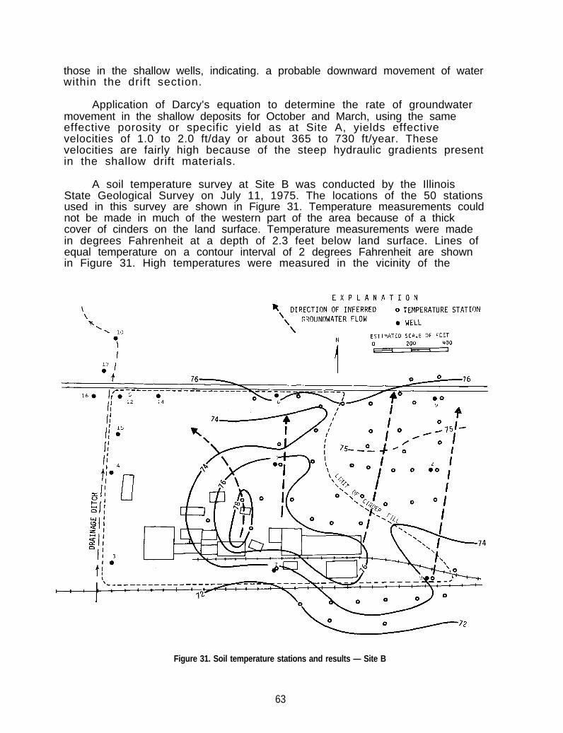
those in the shallow wells, indicating. a probable downward movement of waterwithin the drift section.
Application of Darcy's equation to determine the rate of groundwatermovement in the shallow deposits for October and March, using the sameeffective porosity or specific yield as at Site A, yields effectivevelocities of 1.0 to 2.0 ft/day or about 365 to 730 ft/year. Thesevelocities are fairly high because of the steep hydraulic gradients presentin the shallow drift materials.
A soil temperature survey at Site B was conducted by the IllinoisState Geological Survey on July 11, 1975. The locations of the 50 stationsused in this survey are shown in Figure 31. Temperature measurements couldnot be made in much of the western part of the area because of a thickcover of cinders on the land surface. Temperature measurements were madein degrees Fahrenheit at a depth of 2.3 feet below land surface. Lines ofequal temperature on a contour interval of 2 degrees Fahrenheit are shownin Figure 31. High temperatures were measured in the vicinity of the
Figure 31. Soil temperature stations and results — Site B
63
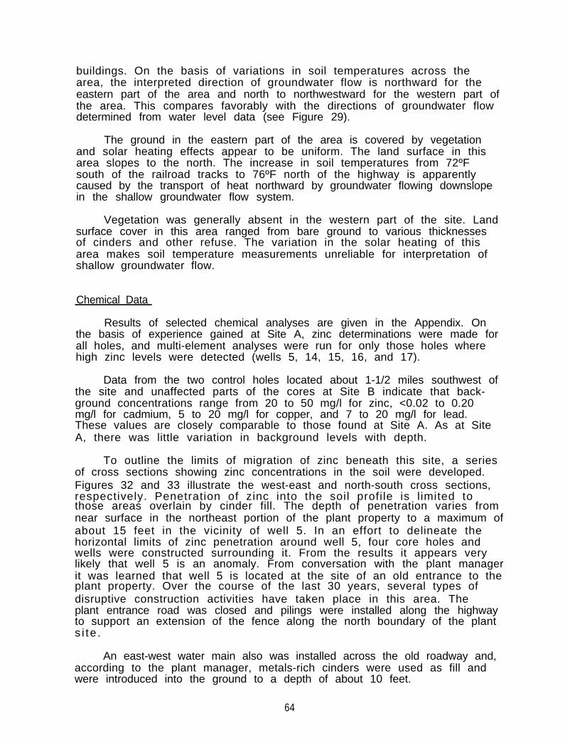
buildings. On the basis of variations in soil temperatures across thearea, the interpreted direction of groundwater flow is northward for theeastern part of the area and north to northwestward for the western part ofthe area. This compares favorably with the directions of groundwater flowdetermined from water level data (see Figure 29).
The ground in the eastern part of the area is covered by vegetationand solar heating effects appear to be uniform. The land surface in thisarea slopes to the north. The increase in soil temperatures from 72ºFsouth of the railroad tracks to 76ºF north of the highway is apparentlycaused by the transport of heat northward by groundwater flowing downslopein the shallow groundwater flow system.
Vegetation was generally absent in the western part of the site. Landsurface cover in this area ranged from bare ground to various thicknessesof cinders and other refuse. The variation in the solar heating of thisarea makes soil temperature measurements unreliable for interpretation ofshallow groundwater flow.
Chemical Data
Results of selected chemical analyses are given in the Appendix. Onthe basis of experience gained at Site A, zinc determinations were made forall holes, and multi-element analyses were run for only those holes wherehigh zinc levels were detected (wells 5, 14, 15, 16, and 17).
Data from the two control holes located about 1-1/2 miles southwest ofthe site and unaffected parts of the cores at Site B indicate that back-ground concentrations range from 20 to 50 mg/l for zinc, <0.02 to 0.20mg/l for cadmium, 5 to 20 mg/l for copper, and 7 to 20 mg/l for lead.These values are closely comparable to those found at Site A. As at SiteA, there was little variation in background levels with depth.
To outline the limits of migration of zinc beneath this site, a seriesof cross sections showing zinc concentrations in the soil were developed.Figures 32 and 33 illustrate the west-east and north-south cross sections,respectively. Penetration of zinc into the soil profile is l imited tothose areas overlain by cinder fill. The depth of penetration varies fromnear surface in the northeast portion of the plant property to a maximum ofabout 15 feet in the vicinity of well 5. In an effort to delineate thehorizontal limits of zinc penetration around well 5, four core holes andwells were constructed surrounding it. From the results it appears verylikely that well 5 is an anomaly. From conversation with the plant managerit was learned that well 5 is located at the site of an old entrance to theplant property. Over the course of the last 30 years, several types ofdisruptive construction activities have taken place in this area. Theplant entrance road was closed and pilings were installed along the highwayto support an extension of the fence along the north boundary of the plants i te .
An east-west water main also was installed across the old roadway and,according to the plant manager, metals-rich cinders were used as fill andwere introduced into the ground to a depth of about 10 feet.
64
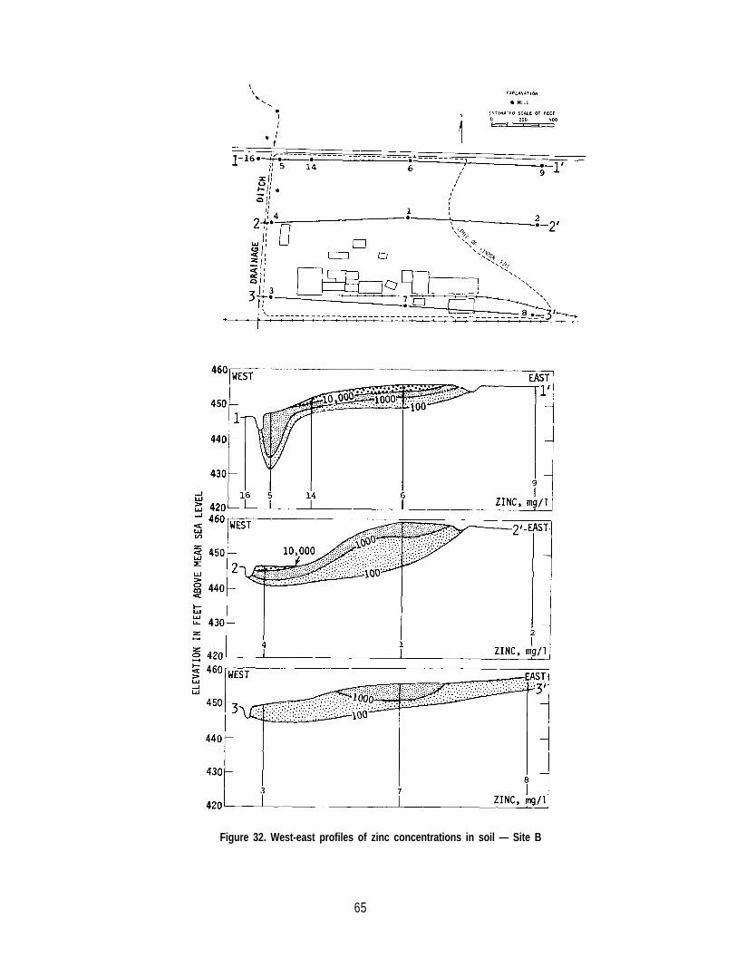
Figure 32. West-east profiles of zinc concentrations in soil — Site B
65
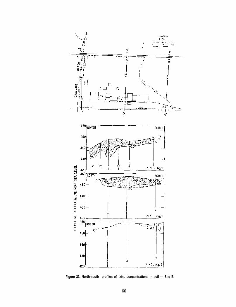
Figure 33. North-south profiles of zinc concentrations in soil — Site B
66
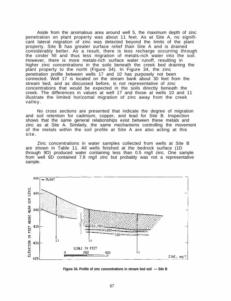
Aside from the anomalous area around well 5, the maximum depth of zincpenetration on plant property was about 11 feet. As at Site A, no signifi-cant lateral migration of zinc was detected beyond the limits of the plantproperty. Site B has greater surface relief than Site A and is drainedconsiderably better. As a result, there is less recharge occurring throughthe cinder fill and thus less migration of metals-rich water into the soil.However, there is more metals-rich surface water runoff, resulting inhigher zinc concentrations in the soils beneath the creek bed draining theplant property to the north (Figure 34). In Figure 34, the zincpenetration profile between wells 17 and 10 has purposely not beenconnected. Well 17 is located on the stream bank about 30 feet from thestream bed, and as discussed before, is not representative of zincconcentrations that would be expected in the soils directly beneath thecreek. The differences in values at well 17 and those at wells 10 and 11illustrate the limited horizontal migration of zinc away from the creekval ley.
No cross sections are presented that indicate the degree of migrationand soil retention for cadmium, copper, and lead for Site B. Inspectionshows that the same general relationships exist between these metals andzinc as at Site A. Similarly, the same mechanisms controlling the movementof the metals within the soil profile at Site A are also acting at thiss i te .
Zinc concentrations in water samples collected from wells at Site Bare shown in Table 11. All wells finished at the bedrock surface (1Dthrough 9D) produced water containing less than 0.5 mg/l zinc. One samplefrom well 6D contained 7.8 mg/l zinc but probably was not a representativesample.
Figure 34. Profile of zinc concentrations in stream bed soil — Site B
67
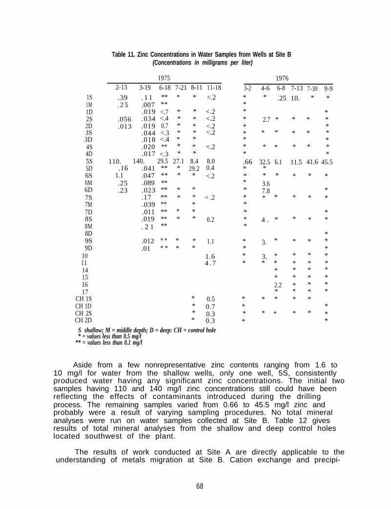
**
**
****
1S .39 . 1 1 ** * * <.21M . 2 5 .007 **1D .019 <.7 * * <.22S .056 .034 <.4 * * <.22D .013 .019 0.7 * * <.23S3D
.044 <.3 * * <.2
.018 <.4 * *4S .020 ** * * <.24D .017 <.3 * *5S 110. 140. 29.5 27.1 8.4 8.05D .16 .041 ** * 29.2 0.46S 1.1 .047 ** * * <.26M .25 .089 **6D .23 .023 ** * *7S .17 ** * * < .27M .039 ** *7D .011 ** * *8S .019 ** * * 0.28M . 2 1 **8D9S .012 * * * * 1.19D .01 * * * *
10 1.611 4 . 714151617
CH 1S * 0.5CH 1D * 0.7CH 2S * 0.3CH 2D * 0.3
S shallow; M = middle depth; D = deep: CH = control hole* = values less than 0.5 mg/l
** = values less than 0.1 mg/l
Table 11. Zinc Concentrations in Water Samples from Wells at Site B(Concentrations in milligrams per liter)
19752-13 3-19 6-18 7-21 8-11 11-18
1976
3-2*********.66*********
4-6 6-8 7-13 7-30 9-9* .25 10. * *
2.7 *
* *
* *
32.5 6.1** *3.67.8* *
4 . *
3. *
3. ** *
**2.2*
* *
* *
** * *
** * *
** * *
*11.5 41.6 45.5
*
*
*
*
*******
*
*
*
*
*
*******
*
*
**
**
*********
***
Aside from a few nonrepresentative zinc contents ranging from 1.6 to10 mg/l for water from the shallow wells, only one well, 5S, consistentlyproduced water having any significant zinc concentrations. The initial twosamples having 110 and 140 mg/l zinc concentrations still could have beenreflecting the effects of contaminants introduced during the drillingprocess. The remaining samples varied from 0.66 to 45.5 mg/l zinc andprobably were a result of varying sampling procedures. No total mineralanalyses were run on water samples collected at Site B. Table 12 givesresults of total mineral analyses from the shallow and deep control holeslocated southwest of the plant.
The results of work conducted at Site A are directly applicable to theunderstanding of metals migration at Site B. Cation exchange and precipi-
68
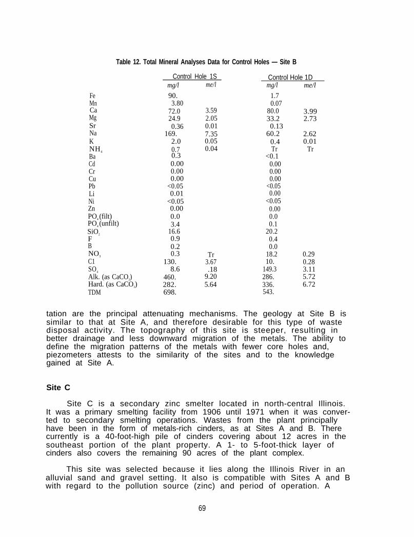
FeMnCaMgSrNaKNH4
BaCdCrCuPbLiNiZnPO4 (filt)PO4 (unfilt)SiO2
FBNO3
C1SO4
Alk. (as CaCO3)Hard. (as CaCO3)TDM
Control Hole 1Smg/l
90.3.80
72.024.90.36
169.2.00.70.30.000.000.00
<0.050.01
<0.050.00
me/l
3.592.050.017.350.050.04
Table 12. Total Mineral Analyses Data for Control Holes — Site B
Control Hole 1Dmg/l me/l
0.03.4
16.60.90.20.3
130.8.6
460.282.698.
Tr3.67.18
9.205.64
1.70.07
80.033.20.13
60.20.4Tr
<0.10.000.000.00
<0.050.00
<0.050.000.00.1
20.20.40.0
18.210.
149.3286.336.543.
3.992.73
2.620.01
Tr
0.290.283.115.726.72
tation are the principal attenuating mechanisms. The geology at Site B issimilar to that at Site A, and therefore desirable for this type of wastedisposal activity. The topography of this site is steeper, resulting inbetter drainage and less downward migration of the metals. The ability todefine the migration patterns of the metals with fewer core holes and,piezometers attests to the similarity of the sites and to the knowledgegained at Site A.
Site C
Site C is a secondary zinc smelter located in north-central Illinois.It was a primary smelting facility from 1906 until 1971 when it was conver-ted to secondary smelting operations. Wastes from the plant principallyhave been in the form of metals-rich cinders, as at Sites A and B. Therecurrently is a 40-foot-high pile of cinders covering about 12 acres in thesoutheast portion of the plant property. A 1- to 5-foot-thick layer ofcinders also covers the remaining 90 acres of the plant complex.
This site was selected because it lies along the Illinois River in analluvial sand and gravel setting. It also is compatible with Sites A and Bwith regard to the pollution source (zinc) and period of operation. A
69
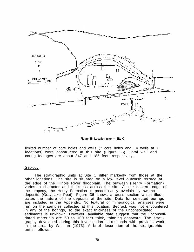
Figure 35. Location map — Site C
limited number of core holes and wells (7 core holes and 14 wells at 7locations) were constructed at this site (Figure 35). Total well andcoring footages are about 347 and 185 feet, respectively.
Geology
The stratigraphic units at Site C differ markedly from those at theother locations. The site is situated on a low level outwash terrace atthe edge of the Illinois River floodplain. The outwash (Henry Formation)varies in character and thickness across the site. At the eastern edge ofthe property, the Henry Formation is predominantly overlain by swampdeposits (Grayslake Peat). Figure 36 shows a cross section which illus-trates the nature of the deposits at the site. Data for selected boringsare included in the Appendix. No textural or mineralogical analyses wererun on the samples collected at this location. Bedrock was not encounteredin any of the borings, so the exact thickness of the unconsolidatedsediments is unknown. However, available data suggest that the unconsoli-dated materials are 50 to 100 feet thick, thinning eastward. The strati-graphy developed during this investigation corresponds with previous workin the area by Willman (1973). A brief description of the stratigraphicunits follows.
70
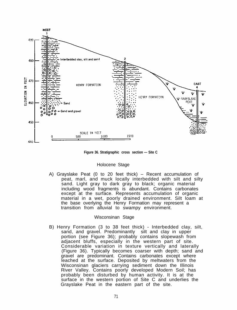
Figure 36. Stratigraphic cross section — Site C
Holocene Stage
A) Grayslake Peat (0 to 20 feet thick) – Recent accumulation ofpeat, marl, and muck locally interbedded with silt and siltysand. Light gray to dark gray to black; organic materialincluding wood fragments is abundant. Contains carbonatesexcept at the surface. Represents accumulation of organicmaterial in a wet, poorly drained environment. Silt loam atthe base overlying the Henry Formation may represent atransition from alluvial to swampy environment.
Wisconsinan Stage
B) Henry Formation (3 to 38 feet thick) - Interbedded clay, silt,sand, and gravel. Predominantly silt and clay in upperportion (see Figure 36); probably contains slopewash fromadjacent bluffs, especially in the western part of site.Considerable variation in texture vertically and laterally(Figure 36). Typically becomes coarser with depth; sand andgravel are predominant. Contains carbonates except whereleached at the surface. Deposited by meltwaters from theWisconsinan glaciers carrying sediment down the IllinoisRiver Valley. Contains poorly developed Modern Soil; hasprobably been disturbed by human activity. It is at thesurface in the western portion of Site C and underlies theGrayslake Peat in the eastern part of the site.
71
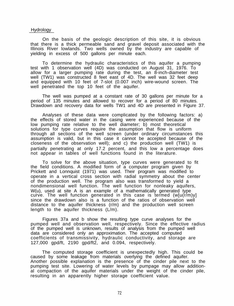
Hydrology
On the basis of the geologic description of this site, it is obviousthat there is a thick permeable sand and gravel deposit associated with theIllinois River lowlands. Two wells owned by the industry are capable ofyielding in excess of 500 gallons per minute each.
To determine the hydraulic characteristics of this aquifer a pumpingtest with 1 observation well (4D) was conducted on August 31, 1976. Toallow for a larger pumping rate during the test, an 8-inch-diameter testwell (TW1) was constructed 8 feet east of 4D. The well was 32 feet deepand equipped with 10 feet of 7-slot (0.007 inch) wire-wound screen. Thewell penetrated the top 10 feet of the aquifer.
The well was pumped at a constant rate of 30 gallons per minute for aperiod of 135 minutes and allowed to recover for a period of 80 minutes.Drawdown and recovery data for wells TW1 and 4D are presented in Figure 37.
Analyses of these data were complicated by the following factors: a)the effects of stored water in the casing were experienced because of thelow pumping rate relative to the well diameter; b) most theoreticalsolutions for type curves require the assumption that flow is uniformthrough all sections of the well screen (under ordinary circumstances thisassumption is valid, but in this case it cannot be accepted because of thecloseness of the observation well); and c) the production well (TW1) ispartially penetrating at only 17.2 percent, and this low a percentage doesnot appear in tables of well functions found in the literature.
To solve for the above situation, type curves were generated to fitthe field conditions. A modified form of a computer program given byPrickett and Lonnquist (1971) was used. Their program was modified tooperate in a vertical cross section with radial symmetry about the centerof the production well. The program also was transformed to yield anondimensional well function. The well function for nonleaky aquifers,W(u), used at site A is an example of a mathematically generated typecurve. The well function generated in this case is termed (w[u(r/m)y]since the drawdown also is a function of the ratios of observation welldistance to the aquifer thickness (r/m) and the production well screenlength to the aquifer thickness (L/m).
Figures 37a and b show the resulting type curve analyses for thepumped well and observation well, respectively. Since the effective radiusof the pumped well is unknown, results of analysis from the pumped welldata are considered only an approximation. The accepted computedcoefficients of transmissivity, hydraulic conductivity, and storage are127,000 gpd/ft, 2190 gpd/ft2, and 0.094, respectively.
The computed storage coefficient is unexpectedly high. This could becaused by some leakage from materials overlying the defined aquifer.Another possible explanation is the presence of the cinder pile next to thepumping test site. Lowering of water levels by pumpage may allow addition-al compaction of the aquifer materials under the weight of the cinder pile,resulting in an apparently higher storage coefficient value.
72
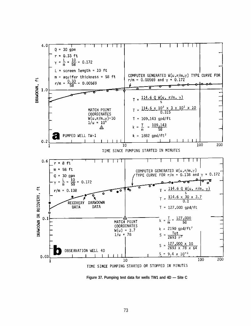
Figure 37. Pumping test data for wells TW1 and 4D — Site C
73
In an effort to detect any possible shallow groundwater contaminationat this site, a series of wells were constructed about 5 to 10 feet belowthe water table surface and another series of wells were installed about 10to 15 feet below that. Water level hydrographs for the shallow and deepwells are presented in Figure 38.
Piezometric surface maps were drawn for each round of water levelmeasurements made. Figures 39a and b illustrate the high and low waterlevel configurations for June 1976 and October 1976, respectively. Thegeneral direction of groundwater movement is to the south toward thebackwater lake and the Illinois River.
Water levels in the deeper wells varied in response to precipitationin a fashion similar to that of the shallow wells. At wells 1 and 2 thevertical movement of water in the drift materials is downward. At allother sites, those closer to the river, the direction of vertical movementis upward. Maximum and minimum water levels for all wells at Site C aresummarized in Table 13.
To determine the rate of groundwater movement Darcy's equation wasapplied as at Site A. On the basis of data presented by Todd (1967), aneffective porosity or specific yield of 0.20 was assumed for the aquifermaterials. The average rates of movement for June and October 1976 were 23and 18 ft/day, respectively. These relatively high rates of groundwatermovement were to be expected in a permeable sand and gravel aquifer of thistype
A soil temperature survey was made at Site C on April 14 and 21,1976. The locations of the 44 stations are shown in Figure 40. Alltemperature readings were normalized to the April 14 conditions. The soiltemperatures were measured at a depth of 2.3 feet and corrected for depthto the water table by methods given by Cartwright (1968). Lines of equaltemperature on a contour interval of two degrees Fahrenheit are shown inFigure 40. High soil temperatures were measured in the area surroundingthe complex of industrial buildings. High soil temperatures measured inlow ground south of the high mound of cinders are caused by groundwaterdischarge. At the season of the year when the soil temperaturemeasurements were made, a warm anomaly is expected in areas of groundwaterdischarge. Groundwater discharge in the vicinity of the cinder pile may bereceiving contributions from the regional flow system as well as fromlocally mounded groundwater in the cinder pile. Groundwater discharge fromthe cinder pile may be highly contaminated.
The inferred direction of groundwater flow for the study area, asinterpreted from the soil temperature, is southward toward the lake. Thiscompares favorably with the direction of groundwater movement determinedfrom water level data (see Figure 39).
Chemical Data
In addition to the analyses of data for geologic interpretation,chemical analyses of the core samples were conducted to define the migra-tion characteristics of the suspected contaminants through the sandy soil
74
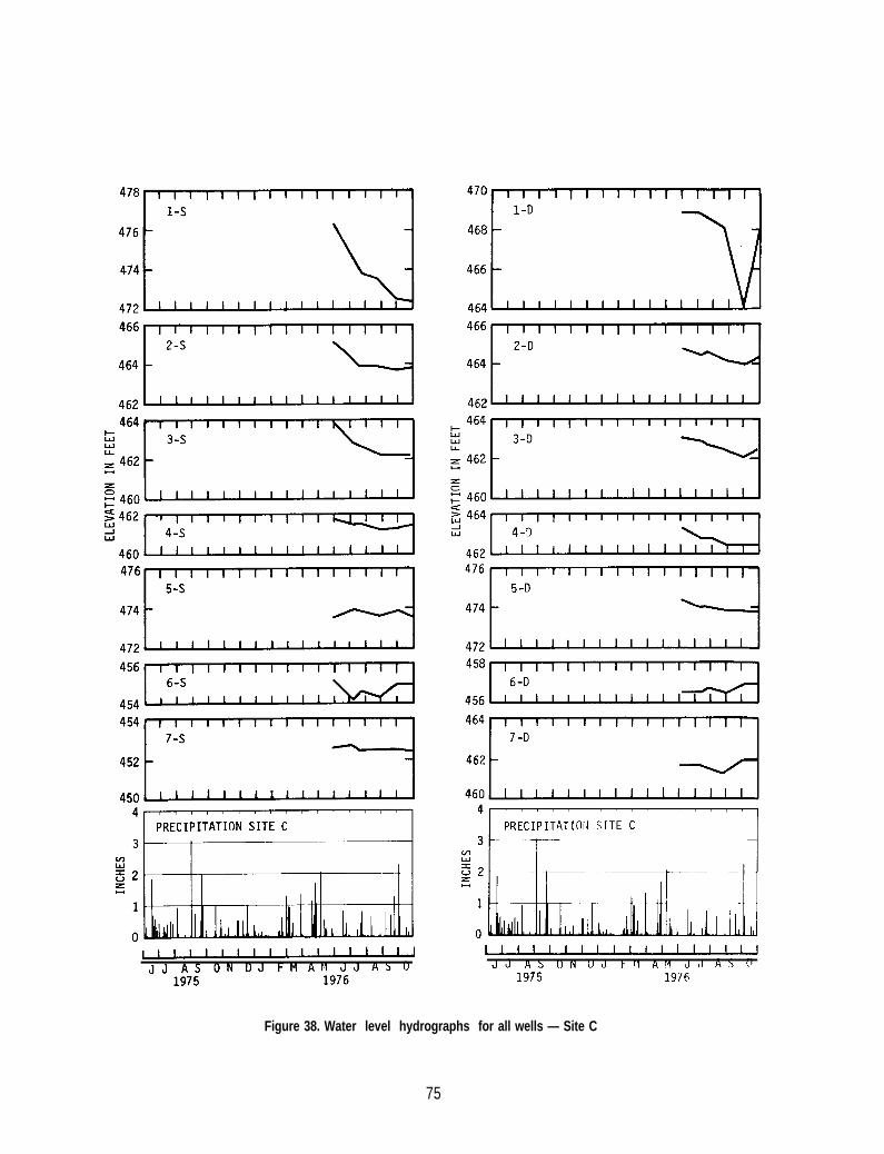
Figure 38. Water level hydrographs for all wells — Site C
75
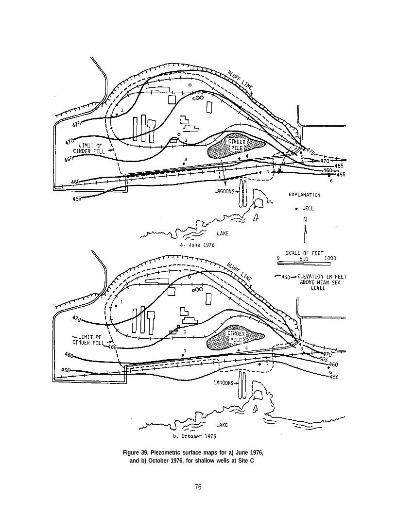
Figure 39. Piezometric surface maps for a) June 1976,and b) October 1976, for shallow wells at Site C
76
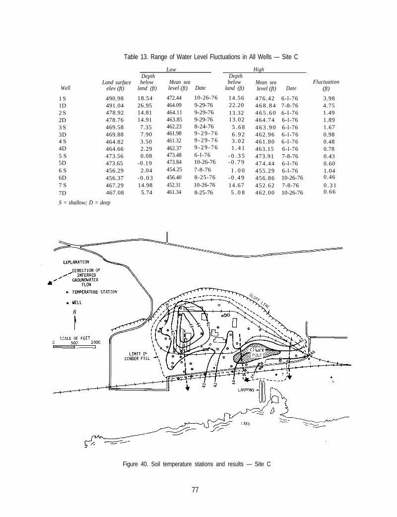
Table 13. Range of Water Level Fluctuations in All Wells — Site C
Low High
Land surfaceWell elev (ft)
1 S 490.981D 491.042 S 478.922D 478.763 S 469.583D 469.884 S 464.824D 464.665 S 473.565D 473.656 S 456.296D 456.377 S 467.297D 467.08
S = shallow; D = deep
Depthbelow
land (ft)
18.5426.9514.8114.917.357.903.502.290.08
-0.192.04
- 0 . 0 314.98
5.74
Mean sealevel (ft) Date
472.44 10-26-76464.09 9-29-76464.11 9-29-76463.85 9-29-76462.23 8-24-76461.98 9 - 2 9 - 7 6461.32 9 - 2 9 - 7 6462.37 9 - 2 9 - 7 6473.48 6-l-76473.84 10-26-76454.25 7-8-76456.40 8-25-76452.31 10-26-76461.34 8-25-76
Depthbelow
land (ft)
14.5622.2013.3213.02
5 . 6 86 . 9 23 . 0 21 . 4 1
- 0 . 3 5- 0 . 7 9
1 . 0 0- 0 . 4 914.675 . 0 8
Mean sea Fluctuationlevel (ft) Date (ft)
476.42 6-l-76 3.984 6 8 . 8 4 7-8-76 4.754 6 5 . 6 0 6-l-76 1.49464.74 6-l-76 1.894 6 3 . 9 0 6-l-76 1.67462.96 6-l-76 0.98461.80 6-l-76 0.48463.15 6-l-76 0.78473.91 7-8-76 0.43474.44 6-l-76 0.60455.29 6-l-76 1.04456.86 10-26-76 0.46
452.62 7-8-76 0 . 3 1462.00 10-26-76 0.66
Figure 40. Soil temperature stations and results — Site C
77
land the effectiveness of these soils in retaining the metal contaminants.Selected analyses are given in the Appendix. As at sites A and B, fourelements -- zinc, cadmium, copper, and lead -- were routinely determined.
No control hole was constructed at this site because of the limitedtime and money available. However, data from the lower segments of allholes at this site suggest that the background concentrations found in thecontrol holes at Sites A and B also are valid at this site. Zinc concen-trations in the lower portions of the seven core holes ranged from about 13to 75 mg/l, cadmium from less than 0.6 to 0.90 mg/l, copper from about 10to 25 mg/l, and lead from less than 4.0 to 90 mg/l.
The number and locations of core holes at this site were not adequateto define the limits of horizontal migration of the metals in the soil.However, the vertical migration patterns are very similar to those at SitesA and B.
Holes 1, 2, and 3 are located on relatively upland portions of theplant complex. Zinc concentrations in excess of 10,000 mg/l were presentin the cinder fill material at the surface. Below the fill, zinc concen-trations generally decrease downward through the soil profile in whichcarbonates have been leached. Cation exchange is the major mechanism ofattenuation in this interval.
Below the zone of leaching, carbonates are present, and the pH isassumed to be about 7 to 8. The increase in soil pH causes precipitationto be an important factor in attenuation and is reflected by an increase inzinc concentrations. Examination of the core samples indicates accumula-tions of zinc carbonate in samples with extremely high zinc levels.
The clays present in the fine-grained surficial geologic material areresponsible for a rapid decrease in zinc concentrations just below thecinder fill material, just as at Sites A and B. However, the Henry Forma-tion becomes coarse grained with depth, and appears to be less effective inattenuating zinc movement by cation exchange. The zinc concentrations dropoff quickly to background levels below a depth of 16 to 17 feet as a resultof the combined action of cation exchange and precipitation.
Holes 4, 5, and 7 also are similar to each other. At each of theselocations the fill materials are underlain by the Grayslake Peat, andmigration into these highly organic materials is minimal. Information forhole 4 indicates that in addition to cation exchange, soil pH also is amajor factor contributing to attenuation. Hole 6 is lowland swampy areawith the grayslake peat at the surface and extending to a depth of about 19feet. The repeated inundation of this location with high metal contentsurface water has resulted in zinc migration to a depth of about 6 feetinto the peat. Analyses of the lake bottom sediments south of the plantindicate that large quantities of heavy metals have left the plant site bysurface water mechanisms (Table 14). The metal contents of the lake bottomsediments can be compared with those of the stream bottom sediments atSites A and B.
78
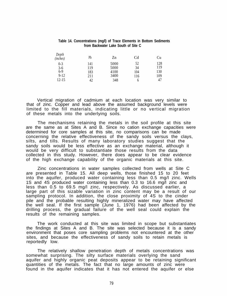
Table 14. Concentrations (mg/l) of Trace Elements in Bottom Sedimentsfrom Backwater Lake South of Site C
Depth(inches) Pb Zn Cd Cu
0-3 141 5000 52 1283-6 119 5000 34 1196-9 183 4100 104 1309-12 211 3400 116 109
12-15 42 348 6 47
Vertical migration of cadmium at each location was very similar tothat of zinc. Copper and lead above the assumed background levels werelimited to the fil l materials, indicating little or no vertical migrationof these metals into the underlying soils.
The mechanisms retaining the metals in the soil profile at this siteare the same as at Sites A and B. Since no cation exchange capacities weredetermined for core samples at this site, no comparisons can be madeconcerning the relative effectiveness of the sandy soils versus the clays,silts, and tills. Results of many laboratory studies suggest that thesandy soils would be less effective as an exchange material, although itwould be very difficult to substantiate those results from the datacollected in this study. However, there does appear to be clear evidenceof the high exchange capability of the organic materials at this site.
Zinc concentrations in water samples collected from wells at Site Care presented in Table 15. All deep wells, those finished 15 to 20 feetinto the aquifer, produced water containing less than 0.5 mg/l zinc. Wells1S and 4S produced water containing less than 0.3 to 16.6 mg/l zinc andless than 0.5 to 69.5 mg/l zinc, respectively. As discussed earlier, alarge part of this sizable variation in zinc content may be a result of oursampling protocol. In addition, the close proximity of 4S to the cinderpile and the probable resulting highly mineralized water may have affectedthe well seal. If the first sample (June 1, 1976) had been affected by thedrilling process, the gradual failure of the well seal could explain theresults of the remaining samples.
The work conducted at this site was limited in scope but substantiatesthe findings at Sites A and B. The site was selected because it is a sandyenvironment that poses core sampling problems not encountered at the othersites, and because the effectiveness of sandy soils to retain metals isreportedly low.
The relatively shallow penetration depth of metals concentrations wassomewhat surprising. The silty surface materials overlying the sandaquifer and highly organic peat deposits appear to be retaining significantquantities of the metals. The fact that no large amounts of zinc werefound in the aquifer indicates that it has not entered the aquifer or else
79
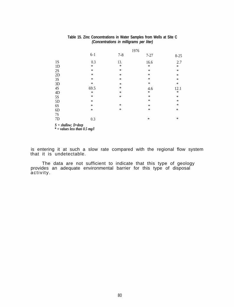
1S1D2S2D3S3D4S4D5S5D6S6D7S7D
Table 15. Zinc Concentrations in Water Samples from Wells at Site C(Concentrations in milligrams per liter)
6-1
0.3*****
69.5***** *
*
*
13.*******
0.3
19767-8 7-27 8-25
16.6 2.7* ** ** ** ** *4.6 12.1* ** ** ** ** *
* *
S = shallow; D=deep* = values less than 0.5 mg/l
is entering it at such a slow rate compared with the regional flow systemthat it is undetectable.
The data are not sufficient to indicate that this type of geologyprovides an adequate environmental barrier for this type of disposalac t iv i ty .
80
SECTION 6
CONCLUSIONS
1. The vertical and horizontal migration patterns of zinc, cadmium,copper, and lead were defined throughout the soil and shallow aquifersystems at Sites A and B. Vertical migration patterns of the same elementswere successfully defined at Site C. In all three cases zinc proved to bethe most mobile, followed by cadmium, copper, and lead, in that order.
2. The contamination which occurred at the three zinc smelters hasbeen contained in the general plant areas by attenuation processes in thesoil, despite the long period of time and the heavy surface loading of thesystems with zinc and other heavy metals. Sites A and B are located inregions generally considered geologically acceptable for such wastedisposal. Site C is in what generally is regarded as a sensitive environ-ment for waste disposal, and may not attenuate constituents that are moremobile than those studied here.
3. Two principal mechanisms control the distribution of zinc andother metals at Sites A, B, and C. These are, in order of dominance,cation exchange and precipitation of insoluble metal compounds as a resultof pH changes in the infiltrating solutions.
4. Soil coring has been demonstrated to be an effective investigativeor research tool in this project. However, proper geologic interpretationand a thorough understanding of soil chemistry is essential to effectiveuse of the technique. Cost analyses and experience gained during thisproject suggest that coring has limited application to routine groundwatermonitoring cases.
5. The use of piezometers or wells for routine monitoring probably ismost cost effective and most easily managed. A limited amount of coresampling would provide data for better vertical and horizontal placement ofalmost all monitoring wells.
6. Proper sampling techniques for collecting representative watersamples from monitoring wells have not been determined. Results of a briefexperiment in this study suggest that variations as great as 45 to 80percent in the chemical constituents of water samples could result fromimproper sampling techniques. Difficulty also was experienced with leakageof surface water through ineffective well seals.
7. Field investigations with geophysical methods show that electricalearth resistivity and soil temperature measurements can be used to gatherinformation rapidly and economically on the lithology of the geologicmaterials, to define the shallow groundwater flow system and to identifypossible zones of contaminated groundwater within the flow system.
8. Geologic environments consisting predominantly of clay, silt, andclay-rich tills have been demonstrated to be effective in retaining themovement of the metals zinc, cadmium, copper, and lead from veryconcentrated inorganic sources.
81
REFERENCES
Berk, W. J., and B. S. Yare. 1977. An Integrated Approach to DelineatingContaminated Ground Water. Ground Water, 15(2): 138-145.
Cartwright, Keros. 1968. Temperature Prospecting for Shallow Glacial andAlluvial Aquifers in Il l inois. Il l inois State Geological SurveyCircular 433.
Cartwright, Keros. 1974. Tracing Shallow Ground-Water Systems by SoilTemperature. Water Resources Research, 10(4): 847-855.
Cartwright, Keros, and M. R. McComas. 1968. Geophysical Surveys in theVicinity of Sanitary Landfills in Northeastern Illinois. GroundWater, 6(5): 23-30.
Cartwright, Keros, and P. C. Reed. 1972. Effect of Deep Glacial-DriftAquifers on Soil Temperatures. Reprint of paper presented at FallMeeting of the Society of Mining Engineers of AIME, Birmingham,Alabama, Preprint No. 72-I-346, 14 p.
Cartwright, Keros, and F. B. Sherman. 1972. Electrical Earth ResistivitySurveying in Landfill Investigations. Proceedings of the 10th AnnualEngineering and Soils Engineering Symposium, Moscow, Idaho,pp. 77-92.
Frost, R. R., and R. A. Griffin. 1977. Effect of pH on Adsorption ofCopper, Zinc, and Cadmium from Landfill Leachate by Clay Minerals.Journal of Environmental Science and Health, Part A, v. 12.
Gibb, J. P., et al. 1981. Procedures for the Selection of RepresentativeWater Quality Data from Monitoring Wells. Illinois State WaterSurvey and State Geological Survey Cooperative Groundwater Report 7,61 p.
Griffin, R. A., et al. 1976. Attenuation of Pollutants in MunicipalLandfill Leachate by Clay Minerals, Part 1 - Column Leaching andField Verification. Environmental Geology Note 78, Illinois StateGeological Survey, 34 p.
Grim, Ralph. 1953. Clay Mineralogy. McGraw Hill Book Company, Inc.,384 p.
Hantush, Mahdi S. 1964. Hydraulics of Wells. In Advances inHydroscience, Vol. 1, edited by Ven Te Chow. Academic Press, NewYork, pp. 284-286.
Prickett, T. A., and C. G. Lonnquist. 1971. Selected Digital ComputerTechniques for Groundwater Resource Evaluation. Illinois State WaterSurvey Bulletin 55, 62 p.
82
Todd, David K. 1967. Ground Water Hydrology. John Wiley and Sons, Inc.,New York, pp. 23-26.
Van Nostrand, R. G., and K. I. Cook. 1966. Interpretation of ResistivityData. Paper 499, U.S. Geological Survey.
Walton, William C. 1962. Selected Analytical Methods for Well and AquiferEvaluation. Illinois State Water Survey Bulletin 49, p. 6.
Willman, H. B. 1973. Geology along the Illinois Waterway - A Basis forEnvironmental Planning. Illinois State Geological SurveyCircular 478.
Willman, H. B., et al. 1975. Handbook of Illinois Stratigraphy. IllinoisState Geological Survey Bulletin 95.
willman, H. B., and J. C. Frye. 1970. Pleistocene Stratigraphy ofIl l inois. Il l inois State Geological Survey Bulletin 94.
83

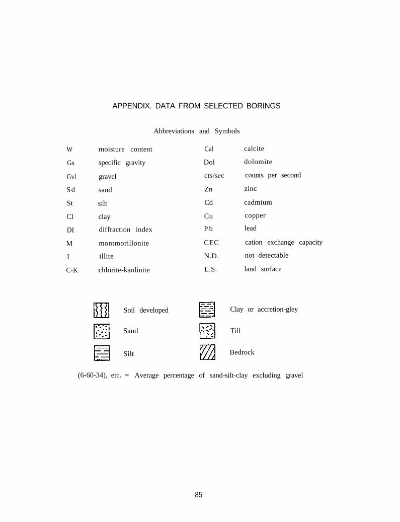
W
Gs
Gvl
Sd
St
Cl
DI
M
I
C-K
APPENDIX. DATA FROM SELECTED BORINGS
Abbreviations and Symbols
moisture content Cal calcite
specific gravity Dol dolomite
gravel cts/sec counts per second
sand
silt
clay
diffraction index
montmorillonite
illite
chlorite-kaolinite
Soil developed
Sand
Silt
Zn
Cd
Cu
P b
CEC
N.D.
L.S.
zinc
cadmium
copper
lead
cation exchange capacity
not detectable
land surface
Clay or accretion-gley
Till
Bedrock
(6-60-34), etc. = Average percentage of sand-silt-clay excluding gravel
85
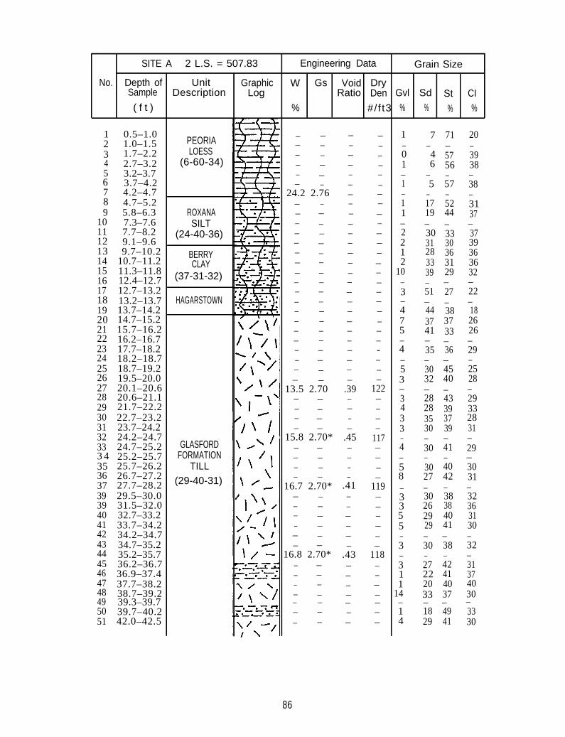
SITE A 2 L.S. = 507.83 Engineering Data Grain Size
No. Depth of Unit Graphic W Gs Void DrySample Description Log Ratio Den Gvl Sd St CI
( f t ) % #/f t3 % % % %
0.5–1.01.0–1.51.7–2.22.7–3.23.2–3.73.7–4.24.2–4.74.7–5.25.8–6.37.3–7.67.7–8.29.1–9.69.7–10.2
10.7–11.211.3–11.812.4–12.712.7–13.213.2–13.713.7–14.214.7–15.215.7–16.216.2–16.717.7–18.218.2–18.718.7–19.219.5–20.020.1–20.620.6–21.121.7–22.222.7–23.223.7–24.224.2–24.724.7–25.225.2–25.725.7–26.226.7–27.227.7–28.229.5–30.031.5–32.032.7–33.233.7–34.234.2–34.734.7–35.235.2–35.736.2–36.736.9–37.437.7–38.238.7–39.239.3–39.739.7–40.242.0–42.5
123456789
1011121314151617181920212223242526272829303132333 43536373939404142434445464748495051
PEORIALOESS
(6-60-34)
ROXANASILT
(24-40-36)
BERRYCLAY
(37-31-32)
HAGARSTOWN
GLASFORDFORMATION
TILL
(29-40-31)
– – – –– – – –– – – –– – – –– – – –– – – –
24.2 2.76 – –– – – –– – – –– – – –– – – –– – – –– – – –– – – –– – – –– – – –– – – –– – – –– – – –– – – –– – – –– – – –– – – -– – – –– – – –– – – –
13.5 2.70 .39 122– – – –– – – –– – – –– – – –
15.8 2.70* .45 117– – – –– – – –– – – –– – – –
16.7 2.70* .41 119– – – –– – – –– – – –– – – –– – – –– – – –
16.8 2.70* .43 118– – – –– – – –– – – –– – – –– – – –– – – –– – – –
1 7 71 20– – – –0 4 57 391 6 56 38– – – –1 5 57 38– – – –1 17 52 311 19 44 37– – – –2 30 33 372 31 30 391 28 36 362 33 31 36
10 39 29 32– – – –3 51 27 22– – – –4 44 38 187 37 37 265 41 33 26– – – –4 35 36 29– – – –5 30 45 253 32 40 28– – – –3 28 43 294 28 39 333 35 37 283 30 39 31– – – –4 30 41 29– – – –5 30 40 308 27 42 31– – – –3 30 38 323 26 38 365 29 40 315 29 41 30– – – –3 30 38 32– – – –3 27 42 311 22 41 371 20 40 40
14 33 37 30– – – –1 18 49 334 29 41 30
86
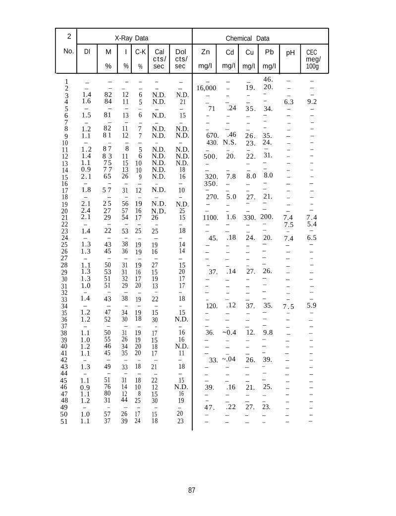
2
No.
123456789
101112131415161718192021222324252627282930313233343536373839404142434445464748495051
Chemical Data
DI
––
1.41.6–
1.5–
1.21.1–
1 .21.41.10.92 .1–
1.8–
2.12.42.1–
1.4–
1.31.3
–1.11.31.31.0–
1.4–
1.21.2–
1.11.01.21.1
–1.3
–1.10.91.11.2–
1.01.1
M
%
––
8284
–81
–828 1
–8 78 3757 765
–5 7
–2 52729
–22
–4345
–50535151
–43–
4752–
50554645–
49–
51768031
–5737
X-Ray Data
I
%
––1211–
13–
1112
–8
11151326–
31–
565754
–53
–3836–
31313229–
38–
3430–
31263435–
33–
31141244–
2639
C-K
%
––65–6–77–56
1010
9–
12–
191617–
25–
1919
–19161720–
19–
1918–
19192020
–18–
1810
825–
1724
Calcts/sec
––
N.D.N.D.–
N.D.–
N.D.N.D.
–N.D.N.D.N.D.N.D.N.D.
–N.D.–
N.D.N.D.26
–25–
1916–
27151913
–22–
1530
–17151817–
21–
22121530–
1518
Dolcts/sec
––
N.D.21–15–
N.D.N.D.
–N.D.N.D.N.D.
1816–10–
N.D.2515–18–1414–15201717–18–15
N.D.–1616
N.D.11–18–15
N.D.1619–2023
Zn
mg/I
–16,000
––71
–––670.430.–
500.––320.350.–270.––
1100.––45.
––––37.
––––120.–––36.–––
33.–––39.––47.––
Cd
mg/I
––––.24–––.46
N.S.–20.
–7.8––5.0––1.6––.18––––.14––––.12–––
~0.4–––
~.04–––.16––.22––
Cu
mg/I
–19.––35.–––26.23.–22.––8.0––27.––
330.––24.––––27.––––37.–––12.–––26.–––21.––27.––
Pb
mg/I
46.20.––34.–––35.24.–31.––8.0––21.––
200.––20.––––26.––––35.–––9.8–––39.–––25.––23.––
pH
–––
6.3––––––––––––––––
7.47.5–
7.4–––––––––
7 . 5–––––––––––––––––
CECmeg/100g
–––
9.2––––––––––––––––
7 .45.4–
6.5–––––––––
5.9–––––––––––––––––
87
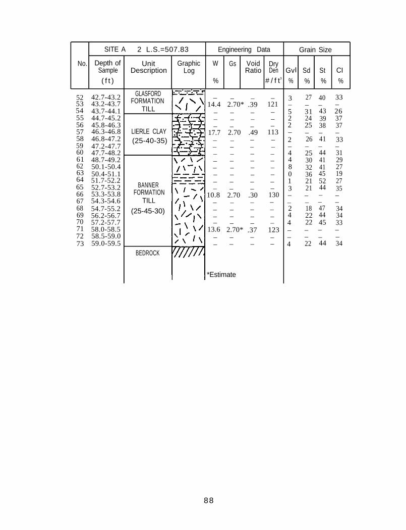
SITE A 2 L.S.=507.83 Engineering Data Grain Size
No. Depth of Unit Graphic W Gs Void DrySample Description Log Ratio Den GvI Sd St CI
( f t ) % # / f t3 % % % %
2.70*–
45.8-46.346.3-46.8
58 – –
47.7-48.2
51.7-52.2
FORMATION
22
58.5-59.0
52 42.7-43.253 43.2-43.754 43.7-44.155 44.7-45.25657
46.8-47.259 47.2-47.76061 48.7-49.262 50.1-50.463 50.4-51.16465 52.7-53.266 53.3-53.867 54.3-54.668 54.7-55.269 56.2-56.770 57.2-57.771 58.0-58.57273 59.0-59.5
GLASFORDFORMATION
TILL
LIERLE CLAY(25-40-35)
BANNER
TILL
(25-45-30)
BEDROCK
– – – –14.4 .39 121
– – –– – – –– – – –
17.7 2.70 .49 113– –– – – –– – – –– – – –– – – –– – – –– – – –– – – –
10.8 2.70 .30 130– – – –– – – –– – – –– – – –
13.6 2.70* .37 123– – – –– – – –
*Estimate
3 27 40 33– – – –5 31 43 262 24 39 372 25 38 37– – – –2 26 41 33– – – –4 25 44 314 30 41 298 32 41 270 36 45 191 21 52 273 21 44 35– – – –– – – –2 18 47 344 44 344 22 45 33– – – –– – – –4 22 44 34
88
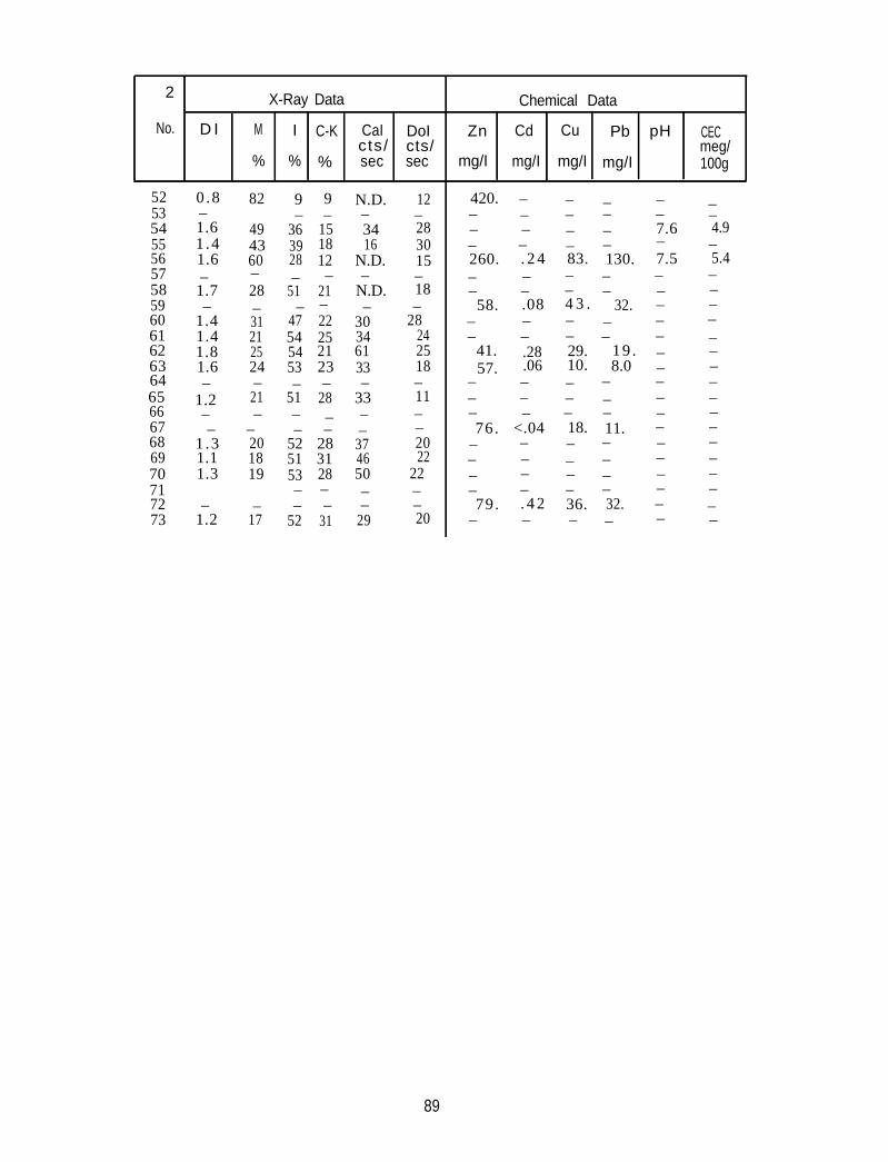
2 X-Ray Data Chemical Data
No. D I M I C-K CaI DoI Zn Cd Cu Pb pH CECcts/ cts/ meg/
% % % sec sec mg/I mg/I mg/I mg/I 100g
52535455565758596061626364656667686970717273
0 .8–1.61 .41.6–1.7–
1.41.41.81.6–
1.2––
1 .31.11.3
–1.2
82
494360–28–31212524–
21–
–201819
–17
9–
363928–
51–
47545453–
51––
525153––
52
9–
151812–
21–22252123–
28––
283128––
31
N.D.–3416
N.D.–
N.D.–
30346133–
33––
374650––
29
12–283015–18–
28242518–11––2022
22––20
420. – – – – –– – – – – –– – – – 7.6 4.9– – – – – –260. . 2 4 83. 130. 7.5 5.4– – – – – –– – – – – –
58. .08 4 3 . 32. – –– – – – – –– – – – – –
41. .28 29. 19 . – –57. .06 10. 8.0 – –
– – – – – –– – – – – –– – – – – –76. <.04 18. 11. – –
– – – – – –– – – – – –– – – – – –– – – – – –79. . 4 2 36. 32. – –
– – – – – –
89
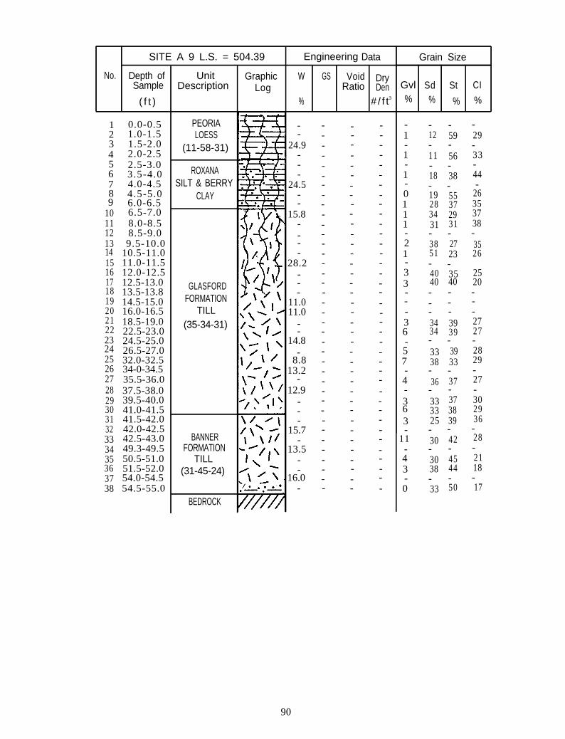
No.
SITE A 9 L.S. = 504.39 Engineering Data Grain Size
Gvl Sd St CI% % % %
0.0-0.51.0-1.51.5-2.02.0-2.52.5-3.03.5-4.04.0-4.54.5-5.0
6.5-7.08.0-8.58.5-9.09.5-10.0
123456789 6.0-6.5
1011121314 10.5-11.015 11.0-11.516 12.0-12.517 12.5-13.018 13.5-13.819 14.5-15.020 16.0-16.521 18.5-19.022 22.5-23.023 24.5-25.024 26.5-27.025 32.0-32.526 34-0-34.527 35.5-36.028 37.5-38.029 39.5-40.030 41.0-41.531 41.5-42.032 42.0-42.533 42.5-43.034 49.3-49.535 50.5-51.036 51.5-52.037 54.0-54.538 54.5-55.0
Depth ofSample
( f t )
Unit GraphicDescription Log
PEORIALOESS
(11-58-31)
--
24.9---
24.5--
15.8----
28.2---
11.011.0
--
14.8-
8.813.2
-12.9
---
15.7-
13.5--
16.0-
ROXANASILT & BERRY
CLAY
-29-33-44-
26353738-3526
2520---2727-2829-27-302936-28-
17
2118-
GLASFORDFORMATION
TILL
(35-34-31)
--------------------------------------
--------------------------------------
--
------------------------------------
-1-1-1-0111-21-33---36-57-4-363-
11-43-0
BANNERFORMATION
TILL(31-45-24)
BEDROCK
W GS Void DryRatio Den
% # / f t3
- -12 59- -11 56- -18 38- -19 5528 3734 2931 31- -38 2751 23- -40 3540 40- -- -- -34 3934 39- -33 3938 33- -36 37- -33 3733 3825 39- -30 42- -30 4538 44- -33 50
90
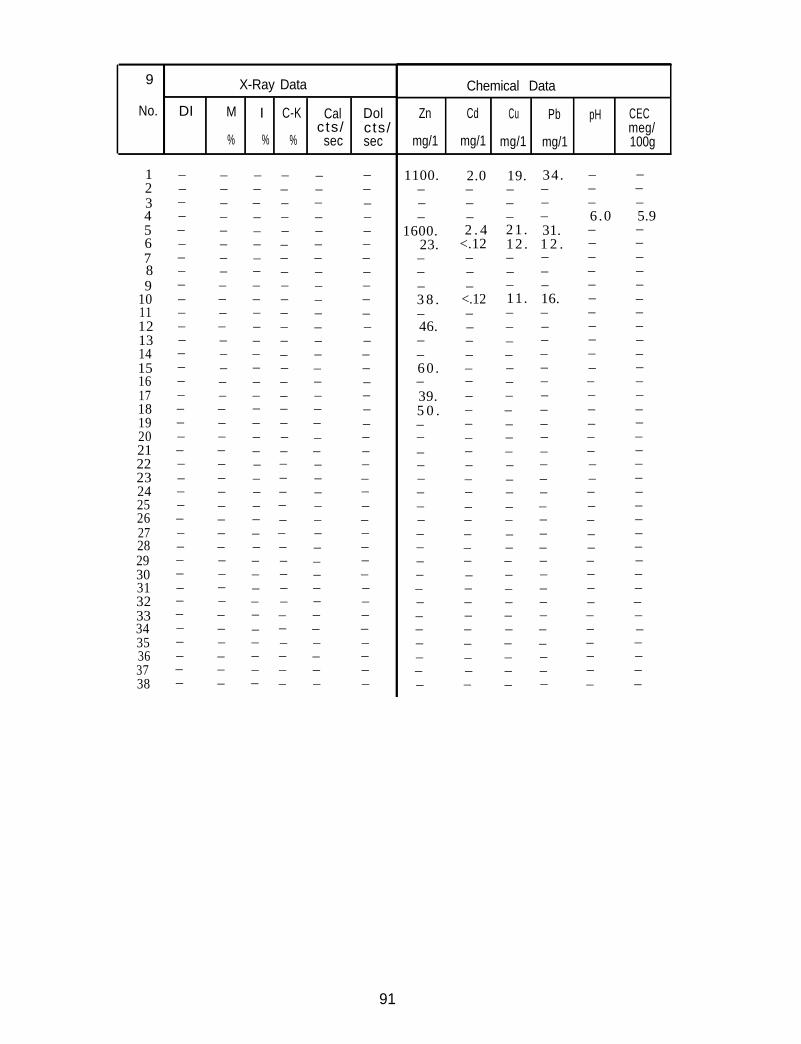
1 – – – – – –2 – – – – – –3 – – – – – –4 – – – – – –5 – – – – – –6 – – – – – –7 – – – – – –8 – – – – – –9 – – – – – –
10 – – – – – –11 – – – – – –12 – – – – – –13 – – – – – –14 – – – – – –15 – – – – – –16 – – – – – –17 – – – – – –18 – – – – – –19 – – – – – –20 – – – – – –21 – – – – – –22 – – – – – –23 – – – – – –24 – – – – – –25 – – – – – –26 – – – – – –27 – – – – – –28 – – – – – –29 – – – – – –30 – – – – – –31 – – – – – –32 – – – – – –33 – – – – – –34 – – – – – –35 – – – – – –36 – – – – – –37 – – – – – –38 – – – – – –
M I C-K Cal Dolcts/ cts/
% % % sec sec
9 X-Ray Data
No. DI
1100. 2.0 19. 34. – –– – – – – –– – – – – –– – – – 6 .0 5.9
1600. 2 . 4 21 . 31. – –23. <.12 12 . 1 2 . – –– – – – – –– – – – – –– – – – – –3 8 . <.12 11. 16. – –– – – – – –46. – – – – –– – – – – –– – – – – –60 . – – – – –– – – – – –39. – – – – –5 0 . – – – – –– – – – – –– – – – – –– – – – – –– – – – – –– – – – – –– – – – – –– – – – – –– – – – – –– – – – – –– – – – – –– – – – – –– – – – – –– – – – – –– – – – – –– – – – – –– – – – – –– – – – – –– – – – – –– – – – – –– – – – – –
Chemical Data
Zn Cd Cu Pb pH
mg/1meg/
mg/1 mg/1 mg/1 100g
CEC
91
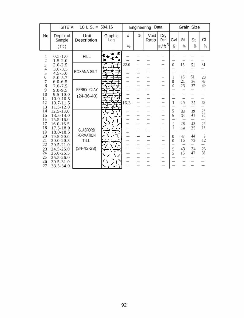
SITE A 10 L.S. = 504.16 Engineering Data Grain Size
No. Depth of Unit Graphic W Gs Void DrySample Description Log Ratio Den Gvl Sd St Cl
( f t ) % # / ft 3 % % % %
1 0.5-1.0 FILL2 1.5-2.03 2.0-2.54 3.0-3.55 4.5-5.0 ROXANA SILT6 5.0-5.77 6.0-6.58 7.0-7.59 9.0-9.5 BERRY CLAY
10 9.5-10.011 10.0-10.5
(24-36-40)
12 10.7-11.513 11.5-12.014 12.5-13.015 13.5-14.016 15.5-16.017 16.0-16.518 17.5-18.019 18.0-18.5 GLASFORD
20 19.5-20.0 FORMATION21 20.0-20.522
TILL20.5-21.0
23 24.5-25.0 (34-43-23)24 25.0-25.525 25.5-26.026 30.5-31.027 33.5-34.0
— — — — — — — —— — — — — — — —
22.0 — — — 0 15 51 34— — — — — — — —— — — — — — — —— — — — 1 16 61 23— — — — 0 21 36 43— — — — 0 23 37 40— — — — — — — —— — — — — — — —— — — — — — — —
16.3 — — — 1 29 35 36— — — — — — — —— — — — 5 33 39 28— — — — 6 33 41 26— — — — — — — —— — — — 3 28 43 29— — — — 1 59 25 16— — — — — — — —— — — — 0 47 44 9— — — — 0 16 72 12— — — — — — — —— — — — 5 43 34 23— — — — 3 15 47 38— — — — — — — —— — — — — — — —— — — — — — — —
92
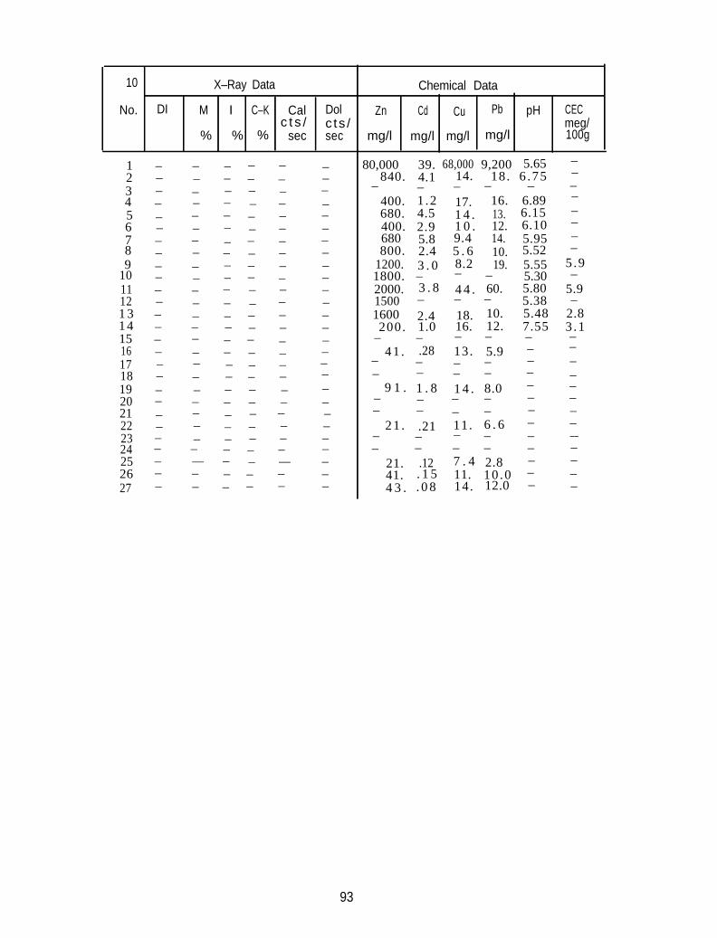
10 X–Ray Data Chemical Data
No. DI M I C–K Cal Dol Zn Cd Cu Pb pH CECc t s / c ts / meg/
% % % sec sec mg/l mg/l mg/l mg/l 100g
840.1 – – – – – –2 – – – – – –3 – – – – – –4 – – – – – –5 – – – – – –6 – – – – – –7 – – – – – –8 – – – – – –9 – – – – – –
10 – – – – – –11 – – – – – –12 – – – – – –1 3 – – – – – –14 – – – – – –15 – – – – – –16 – – – – – –17 – – – – – –18 – – – – – –19 – – – – – –20 – – – – – –21 – – – – – –22 – – – – – –23 – – – – – –24 – – – – – –25 – — – – — –26 – – – – – –27 – – – – – –
80,000 39. 68,000 9,200 5.65 –4.1 14. 18. 6 .75 –
– – – – – –400. 1 .2 17. 16. 6.89 –680. 4.5 1 4 . 13. 6.15 –400. 2.9 1 0 . 12. 6.10 –680 5.8 9.4 14. 5.95 –800. 2.4 5 . 6 10. 5.52 –
1200. 3 . 0 8.2 19. 5.55 5 .91800. – – – 5.30 –2000. 3 . 8 4 4 . 60. 5.80 5.91500 – – – 5.38 –1600 2.4 18. 10. 5.48 2.8200. 1.0 16. 12. 7.55 3 .1
– – – – – –41 . – –
–.28 13. 5.9– – – – –
– – – – – –9 1 . 1 . 8 1 4 . 8.0 – –
– – – – – –– – – – – –
21 . 11. 6 . 6 – ––
.21– – – – ––
– – – – – –21. .12 7 . 4 2.8 – –41. . 1 5 11. 10 .0 – –4 3 . . 0 8 14. 12.0 – –
93
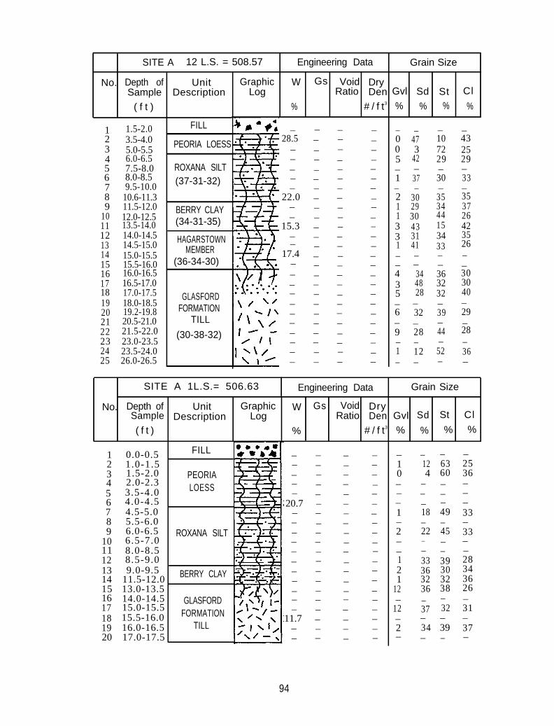
SITE A 12 L.S. = 508.57 Engineering Data Grain Size
No. Depth ofSample
( f t )
Graphic W Gs Void DryLog Ratio Den Gvl Sd St Cl
% # / f t3 % % % %
12
1.5-2.03.5-4.0
3 5.0-5.54 6.0-6.55 7.5-8.06 8.0-8.57 9.5-10.08 10.6-11.39 11.5-12.0
10 12.0-12.511 13.5-14.012 14.0-14.513 14.5-15.014 15.0-15.515 15.5-16.016 16.0-16.517 16.5-17.018 17.0-17.519 18.0-18.520 19.2-19.821 20.5-21.022 21.5-22.023 23.0-23.524 23.5-24.025 26.0-26.5
UnitDescription
FILL
PEORIA LOESS
ROXANA SILT(37-31-32)
BERRY CLAY(34-31-35)
HAGARSTOWNMEMBER
(36-34-30)
– – – –28.5 – – –
– – – –– – – –– – – –– – – –– – – –
22.0 – – –– – – –– – – –
15.3 – – –– – – –
– – ––17.4 – – –
– – – –– – – –
– – ––– – – –– – – –– – – –– – – –– – – –– – – –– – – –– – – –
GLASFORDFORMATION
TILL
(30-38-32)
SITE A 1L.S.= 506.63 Engineering Data Grain Size
No. Depth ofSample
( f t )
Gvl Sd St Cl
% % % %
2 1.0-1.53 1.5-2.0
3.5-4.06 4.0-4.5
4.5-5.05.5-6.06.0-6.56.5-7.0
12 8.5-9.013 9.0-9.514 11.5-12.015 13.0-13.516 14.0-14.517 15.0-15.518 15.5-16.01920 17.0-17.5
1 0.0-0.5
4 2.0-2.35
789
1011 8.0-8.5
16.0-16.5
– –0 470 35 42– –1 37– –2 301 291 303 433 311 41– –– –4 343 485 28– –6 32– –9 28– –1 12– –
– –10 4372 2529 29– –30 33– –35 3534 3744 2615 4234 3533 26– –– –36 3032 30
4032– –39 29– –44 28– –
52 36– –
Unit Graphic W Gs Void DryDescription Log Ratio Den
% # / f t3
FILL – – – –– – – –
PEORIA – – – –– – –LOESS –– – – –
20.7 – – –– – – –– – – –
ROXANA SILT – – – –– – – –– – – –– – – –
BERRY CLAY – – – –– – – –– – – –
GLASFORD – – – ––FORMATION – – –
11.7 – – –TILL – – – –
– – – –
–10–––1–2––121
12–
12–2–
– –12 634 60
– –– –– –18 49– –22 45– –– –33 3936 3032 3236 38– –37 32– –34 39– –
–2536–––33–33––28343626–31–37–
94
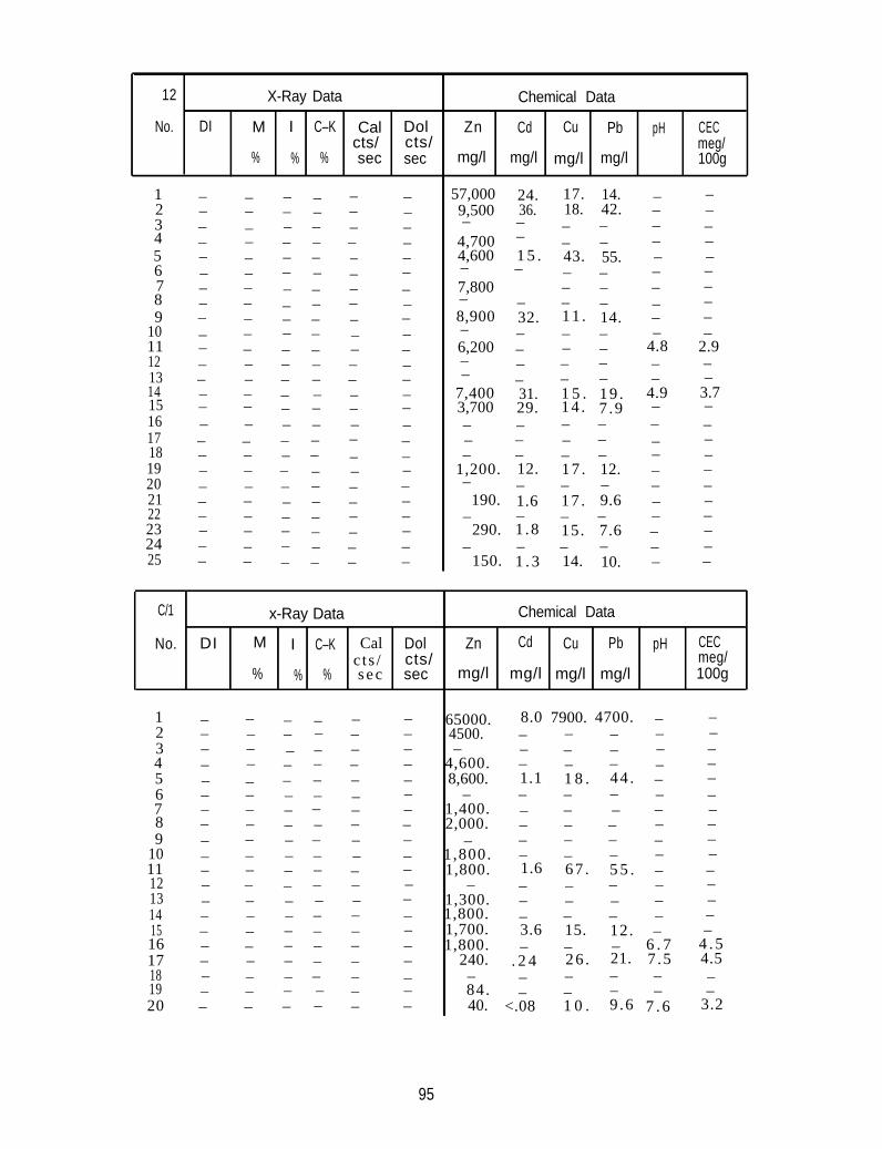
Zn Cd Cu Pb pH CECmeg/100gmg/l mg/l mg/l mg/l
Chemical Data
seccts/Cal
seccts/Dol
X-Ray Data
DI M
%
I
%
C–K
%
12
No.
1 – – – – – –2 – – – – – –3 – – – – – –4 – – – – – –5 – – – – – –6 – – – – – –7 – – – – – –8 – – – – – –9 – – – – – –
10 – – – – – –11 – – – – – –12 – – – – – –13 – – – – – –14 – – – – – –15 – – – – – –16 – – – – – –17 – – – – – –18 – – – – – –19 – – – – – –20 – – – – – –21 – – – – – –22 – – – – – –23 – – – – – –24 – – – – – –25 – – – – – –
57,000 24. 17. 14. – –9,500 36. 18. 42. – –– – – – – –
4,700 – – – – –4,600 1 5 . 43. 55. – –– – – –7,800
– –– – – –
– – – – – –8,900 32. 11 . 14. – –– – – – – –6,200 – – – 4.8 2.9– – – – – –– – – – – –
7,400 31. 1 5 . 19 . 4.9 3.73,700 29. 14 . 7 .9 – –– – – – – –– – – – – –– – – – – –
1,200. 12. 17 . 12. – –– – – – – –
190. 9.6 – ––
1.6 17 .– – – – –
290. 1 .8 15. 7.6 – –– – – – – –
150. 1 . 3 14. 10. – –
Chemical Data
Zn Cd Cu Pb pH CECmeg/
mg/l mg/l mg/l mg/l 100g
65000. 8.0 7900. 4700. – –4500. – – – – –– – – –
4,600.– –– – – – –
8,600. 1.1 1 8 . 44 . – –– – – – – –
1,400. – – – – –2,000. – – – – –
– – – – – –1,800. – – – – –1,800. 1.6 67 . 5 5 . – –
– – – – – –1,300. – – – – –1,800. – – – – –1,700. 3.6 15. 12. – –1,800. – – – 6 . 7 4 . 5
240. . 2 4 26 . 21. 7 .5 4.5– – – – – –84. – – – – –40. <.08 1 0 . 9 .6 7 . 6 3.2
s e c
Calc t s /
M I C–K
C/1
Dolcts/sec% %%
No. DI
x-Ray Data
123456789
1011121314151617181920
– – – – ––
–– – – –
––
– – – – –– – – – – –– – – – – –– – – – – –– – – – – –– – – – – –– – – – – –– – – – – –– – – – – –– – – – – –– – – – – –– – – – – –– – – – – –– – – – – –– – – – ––
–– – – –
––– – – – –
– – – – – –
95
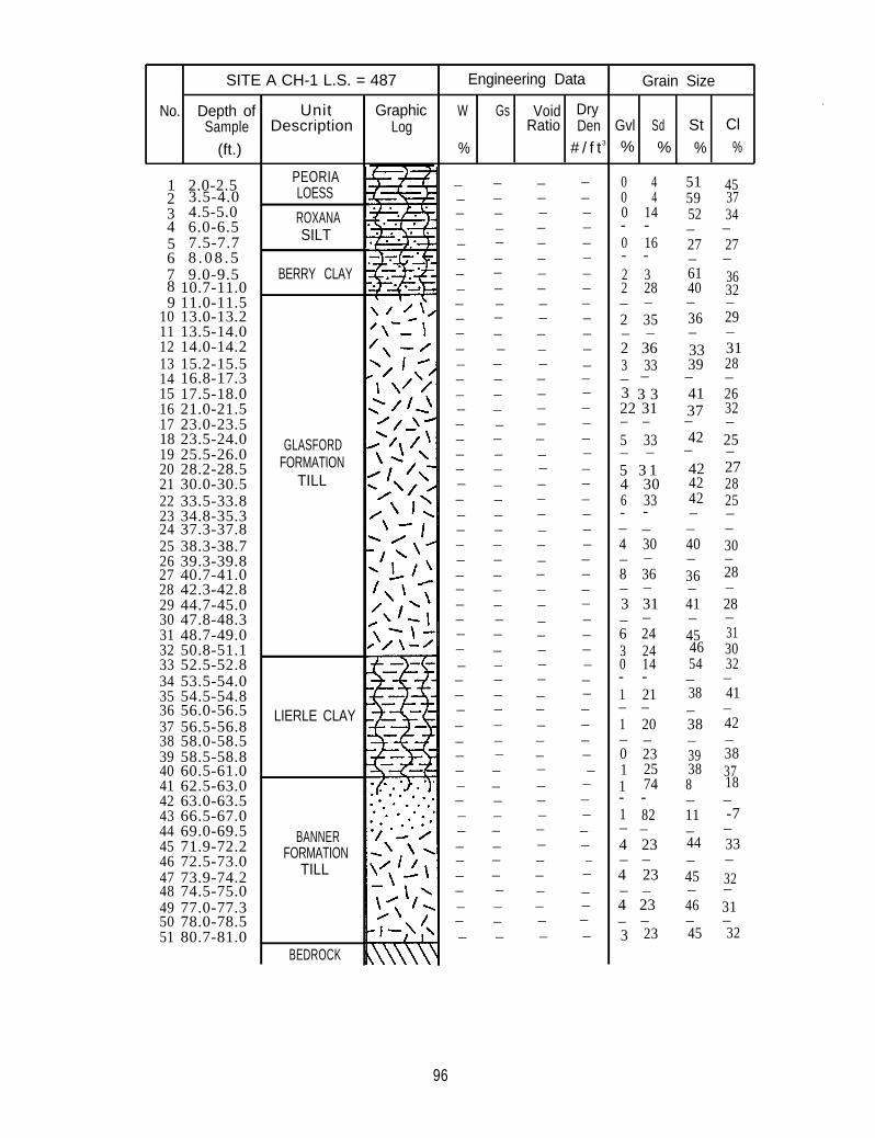
SITE A CH-1 L.S. = 487
No. Depth ofSample
(ft.)
Gvl Sd St Cl
% % % %
1 2.0-2.52 3.5-4.03 4.5-5.04 6.0-6.55 7.5-7.76 8 . 0 8 . 5
8 10.7-11.09 11.0-11.5
10 13.0-13.211 13.5-14.012 14.0-14.2
5159
–
– –7 9.0-9.5
– – –
– – –3339–4137–42–424242
3113 15.2-15.514 16.8-17.315 17.5-18.0
–
16 21.0-21.517 23.0-23.518 23.5-24.019 25.5-26.020 28.2-28.521 30.0-30.522 33.5-33.823 34.8-35.324 37.3-37.825 38.3-38.726 39.3-39.827 40.7-41.028 42.3-42.829 44.7-45.030 47.8-48.331 48.7-49.032 50.8-51.133 52.5-52.834 53.5-54.035 54.5-54.836 56.0-56.537 56.5-56.838 58.0-58.539 58.5-58.840 60.5-61.041 62.5-63.042 63.0-63.543 66.5-67.044 69.0-69.545 71.9-72.246 72.5-73.047 73.9-74.248 74.5-75.049 77.0-77.350 78.0-78.551 80.7-81.0
Unit GraphicDescription Log
PEORIALOESS
ROXANASILT
BERRY CLAY
–
GLASFORDFORMATION
TILL
– – – –– – – –– – – –– – – –– – – –– – – –– – – –– – – –– – – –– – – –– – – –– – – –– – – –– – – –– – – –– – – –– – – –– – – –– – – –– – – –– – – –– – – –– – – –– – – –– – – –– – – –– – – –– – – –– – – –– – – –– – – –– – – –– – – –– – – –– – – –– – – –– – – –– – – –– – – –– – – –– – – –– – – –– – – –– – – –– – – –– – – –– – – – –– – – –– – – –– – – –– – – –
– –27
4 30
– –– – – –
– – –
– – –
–
46
– –
LIERLE CLAY – –
– – –3938
– –
–BANNER
FORMATIONTILL
–
– – –
– – – –
– – – –
BEDROCK
Engineering Data
W Gs Void DryRatio Den
% # / f t3
Grain Size
0 40 40 14- -0 16- -2 32 28
–2 35
–2 363 33– –3 3 322 31– –5 33
–5 3 1
6 33- -
4 30–
8 36–
3 31–
6 243 240 14- -1 21– –1 20
–0 231 251 74- -1 82
–4 23
–4 23
4 23
3 23
52–27
6140
36
40
36
41–45
54
38
38
8
11–44
45
46
45
453734
27
3632
29
28
2632
25
2825
30
28
28–313032
41
42
383718
-7
33
32
31
32
96
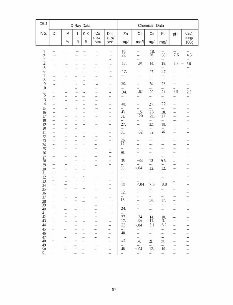
X-Ray Data
Zn
–
Cd Cu Pb pH
mg/l mg/l mg/l mg/l 100gmeg/CEC
Chemical DataCH–1
DI M I C–KNo.
% % % seccts/
Cal
seccts/Dol
– – – – – 18. – 18. – – –– – – – – – 25. – 26. 38. 7.6 4.5– – – – – – – – – – – –– – – – – – 17. .04 14. 18. 7.5 – 5.6– – – – – – – – – – –– – – – – – 17. – 27. 27. – –
–
– – – – – – – – – – – –– – – – – – – – – – – –– – – – – – 20. – 24. 22. – –– – – – – – – – – – – –– – – – – – 34. .62 20. 21. 6.9 2.5– – – – – – – – – – – –– – – – – – – – – – – –– – – – – – 40. – 27. 22. – –– – – – – – – – – – – –– – – – – – 43. 1.5 23. 18. – –– – – – – – 32. .20 21. 17. – –– – – – – – – – – – – –– – – – – – 27. – 22. 18. – –– – – – – – – – – – – –
46.– – – – – – 35. .32 32. – –– – – – – – – – – – – –– – – – – – 26. – – – – –– – – – – – 17. – – – – –– – – – – – – – – – – –– – – – – –
123456789
101112131415161718192021222324252627282930313233343536373839404142434445464748495051
30. – – – – –– – – – – – – – – – – –– – – – – – 35. ~.04 12 9.8 – –– – – – – – – – – – – –– – – – – – 36 <.04 12. 12. – –– – – – – – – – – – – –– – – – – – – – – – – –– – – – – – – – – – – –– – – – – – 13. <.04 7.6 8.8 – –– – – – – – – – – – – –– – – – – – 12. – – – –
––
– – – – – – – – – –18.
–– – – – – – – 14. 17. – –– – – – – – – – – – – –– – – – – – 24. – – – – –– – – – – – – – – – – –– – – – – – 37. .24 14. 10. – –– – – – – – 17. .06 11. 3. – –– – – – – – 23. ~.04 5.1 3.2 – –– – – – – – – – – – – –– – – – – – 48. – – – – –– – – – – – – – – – – –– – – – – –– – – – – – – – – – – –– – – – – – 48. <.04 12. 10. – –– – – – – – – – – – – –
47. .40 21. 22. – –
97
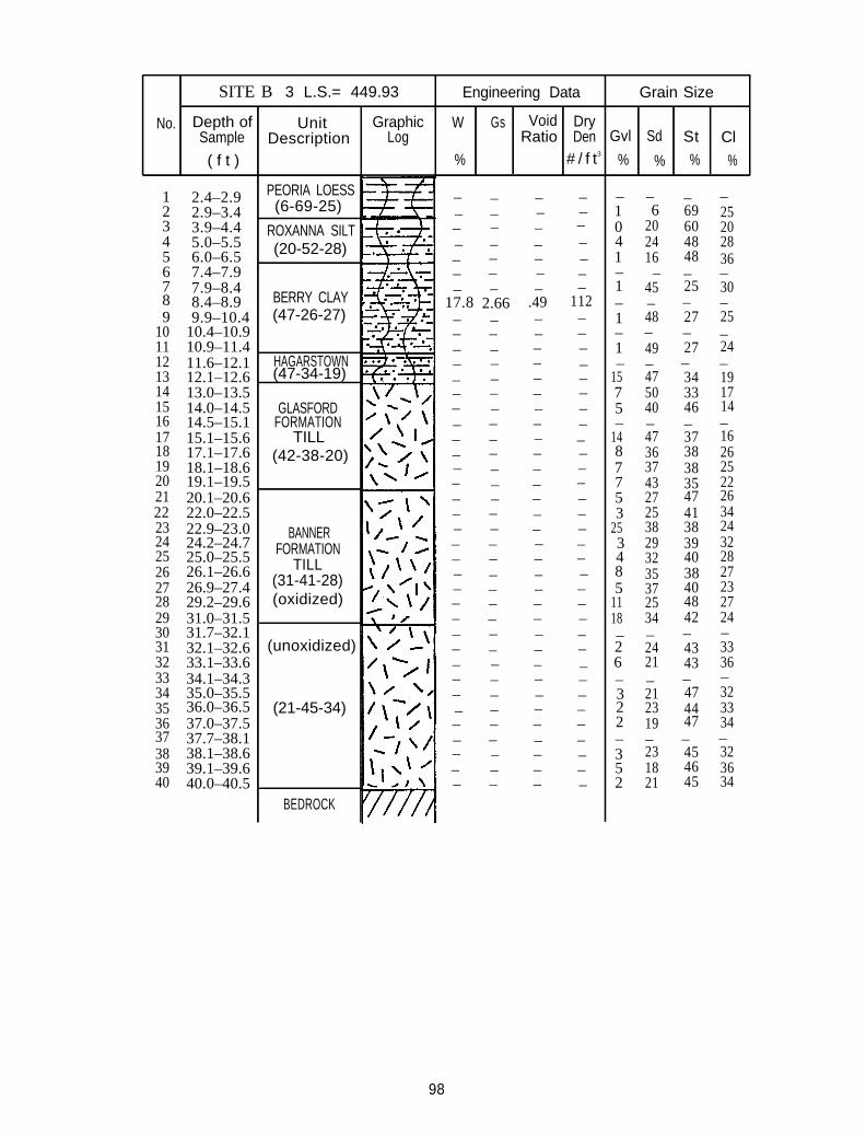
SITE B 3 L.S.= 449.93 Engineering Data Grain Size
No. Depth of Unit Graphic W Gs Void DrySample Description Log Ratio Den Gvl Sd St Cl
( f t ) % # / f t3% % % %
1 2.4–2.92 2.9–3.43 3.9–4.44 5.0–5.55 6.0–6.56 7.4–7.97 7.9–8.48 8.4–8.99 9.9–10.4
10 10.4–10.911 10.9–11.412 11.6–12.113 12.1–12.614 13.0–13.515 14.0–14.516 14.5–15.117 15.1–15.618 17.1–17.619 18.1–18.620 19.1–19.521 20.1–20.622 22.0–22.523 22.9–23.024 24.2–24.725 25.0–25.526 26.1–26.627 26.9–27.428 29.2–29.629 31.0–31.530 31.7–32.131 32.1–32.632 33.1–33.633 34.1–34.334 35.0–35.535 36.0–36.536 37.0–37.537 37.7–38.138 38.1–38.639 39.1–39.640 40.0–40.5
PEORIA LOESS(6-69-25)
ROXANNA SILT(20-52-28)
BERRY CLAY(47-26-27)
HAGARSTOWN(47-34-19)
GLASFORDFORMATION
TILL(42-38-20)
BANNERFORMATION
TILL(31-41-28)(oxidized)
– – – – – – – –– – – – 1 6 69 25– – – – 0 20 60 20– – – – 4 24 48 28– – – – 1 16 48 36– – – – – – – –– – – – 1 45 25 30
17.8 2.66 .49 112 – – – –– – – – 1 48 27 25– – – – – – – –– – – – 1 49 27 24– – – – – – – –– – – – 15 47 34 19– – – – 7 50 33 17– – – – 5 40 46 14– – – – – – – –– – – – 14 47 37 16– – – – 8 36 38 26– – – – 7 37 38 25– – – – 7 43 35 22– – – – 5 27 47 26– – – – 3 25 41 34– – – – 25 38 38 24– – – – 3 29 39 32– – – 4– 32 40 28– – – 8– 35 38 27– – – – 5 37 40 23– – – – 11 25 48 27– – – – 18 34 42 24– – – – – – – –– – 2– – 24 43 33– – – – 6 21 43 36– – – – – – – –– – – – 3 21 47 32– – – – 2 23 44 33
– – 2 19 47 34– –– – – – – – – –– – – – 3 23 45 32– – – – 5 18 46 36– – – 2 45 34– 21
(unoxidized)
(21-45-34)
BEDROCK
98
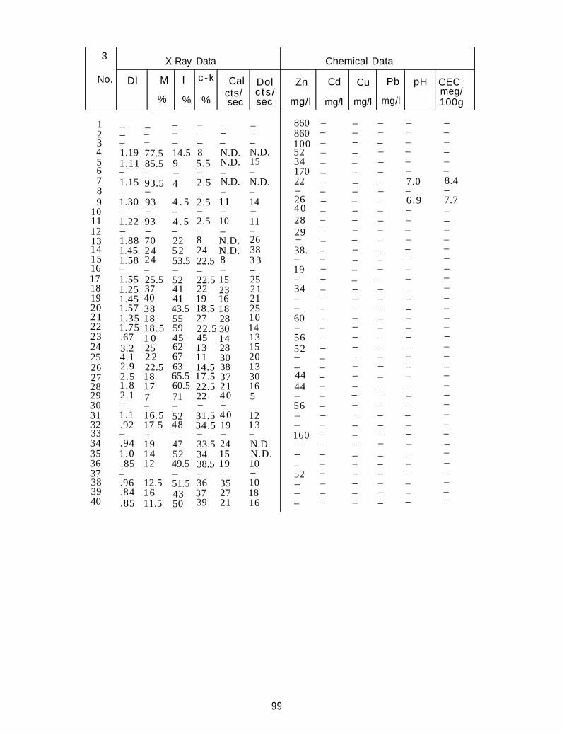
3 X-Ray Data
No. DI M I c-k Cal Dol
%cts /
%cts/
% sec
Chemical Data
Zn Cd Cu Pb pH CECmeg/
sec mg/l mg/l mg/l mg/l 100g
1 – – – – – –2 – – – – – –3 – – – – – –4 1.19 77.5 14.5 8 N.D. N.D. 525 1.11 85.5 9 5.5 N.D. 15 346 – – – – – –7 1.15 93.5 4 2.5 N.D. N.D. 228 – – – – –9
–1.30
–93 4 . 5 2.5 11 14 26
10 – – – – – –11 1.22 93 4 . 5 2.5 10 1112 – – – – – –13 1.88 70 22 8 N.D. 2614 1.45 24 52 24 N.D. 38 38.15 1.58 24 53.5 22.5 8 3 316 – – –17
– – –1.55 25.5 52 22.5 15 25
18 1.25 37 41 22 23 2119 1.45 40 41 19 16 2120 1.57 38 43.5 18.5 18 2521 1.35 18 55 27 28 1022 1.75 18.5 59 22.5 30 1423 .67 1 0 45 45 14 1324 3.2 25 62 13 28 1525 4.1 2 2 67 11 30 2026 2.9 22.5 63 14.5 38 1327 2.5 18 65.5 17.5 37 3028 1.8 17 60.5 22.5 21 1629 2.1 7 71 22 40 5 –30 – – – – –31 1.1 16.5 52 31.5 4 0 1232 .92 17.5 48 34.5 19 1333 – – – – – –34 .94 19 47 33.5 24 N.D.35 1.0 14 52 34 15 N.D.36 .85 12 49.5 38.5 19 1037 – – – – – –38 .96 12.5 51.5 36 35 1039 .84 16 43 37 27 1840 .85 11.5 50 39 21 16
860860100
170
402829–
–19–34––60–5652––4444
56––160–––52–––
– – – – –– – – – –– – – – –– – – – –– – – – –– – – – –– – – 7.0 8.4– – – – –– – – 6.9 7.7– – – – –– – – – –– – – – –– – – – –– – – – –– – – – –– – – – –– – – – –– – – – –– – – – –– – – – –– – – – –– – – – –– – – – –– – – – –– – – – –– – – – –– – – – –– – – – –– – – – –– – – – –– – – – –– – – – –– – – – –– – – – –– – – – –– – – – –– – – – –– – – – –– – – – –– – – – –
99
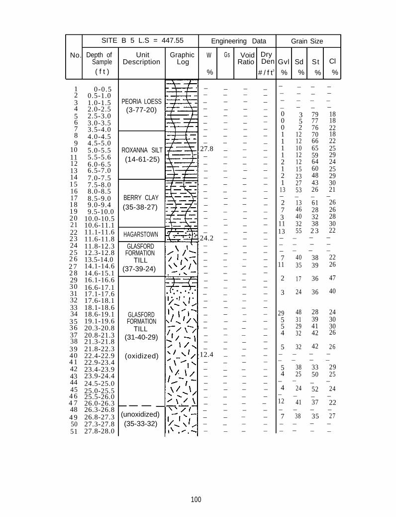
SITE B 5 L.S = 447.55 Engineering Data Grain Size
No. Depth of Unit Graphic W Gs Void DrySample Description Log Ratio Den Gvl Sd St Cl
( f t ) % # / f t3 % % % %
1 0-0.52 0.5-1.03 1.0-1.5 PEORIA LOESS4 2.0-2.55 2.5-3.0
(3-77-20)
6 3.0-3.57 3.5-4.08 4.0-4.59 4.5-5.0
10 5.0-5.5 ROXANNA SILT11 5.5-5.612 6.0-6.5
(14-61-25)
13 6.5-7.014 7.0-7.515 7.5-8.016 8.0-8.517 8.5-9.0 BERRY CLAY18 9.0-9.419 9.5-10.0
(35-38-27)
20 10.0-10.521 10.6-11.122 11.1-11.623 11.6-11.8
HAGARSTOWN
24 11.8-12.3 GLASFORD25 12.3-12.8 FORMATION2 6 13.5-14.0 TILL2 7 14.1-14.62 8 14.6-15.1
(37-39-24)
29 16.1-16.630 16.6-17.131 17.1-17.632 17.6-18.133 18.1-18.634 18.6-19.1 GLASFORD35 19.1-19.6 FORMATION36 20.3-20.8 TILL37 20.8-21.338 21.3-21.8
(31-40-29)
39 21.8-22.340 22.4-22.9 (oxidized)4 1 22.9-23.442 23.4-23.943 23.9-24.444 24.5-25.045 25.0-25.54 6 25.5-26.04 748
26.0-26.326.3-26.8
4 9 26.8-27.3 (unoxidized)50 27.3-27.8 (35-33-32)51 27.8-28.0
– – – – – – – –– – – – – – – –– – – – – – – –– – – – – – – –– – – – 0 3 79 18– – – – 0 5 77 18– – – – 0 2 76 22– – – – 1 12 70 18– – – – 1 12 66 22
27.8 – – – 1 10 65 25– – – – 1 12 59 29– – – – 2 12 64 24– – – – 1 15 60 25– – – – 2 23 48 29– – – – 1 27 43 30– – – – 13 53 26 21– – – – – – – –– – – – 2 13 61 26– – – – 7 46 28 26– – – – 3 40 32 28– – – – 11 32 38 30– – – – 13 55 2 3 22
24.2 – – – – – – –– – – – – – – –– – – – – – – –– – – – 7 40 38 22– – – – 11 35 39 26– – – –– – – – 2 17 36 47– – – –– – – – 3 24 36 40– – – –– – – –– – – – 29 48 28 24– – – – 5 31 39 30– – – – 5 29 41 30– – – – 4 32 42 26– – – –– – – – 5 32 42 26
12.4 – – – – – – –– – – – – – – –– – – – 5 38 33 29– – – – 4 25 50 25– – – – – – – –– – – – 4 24 52 24– – – – – – – –– – – – 12 41 37 22– – – – – – – –– – – – 7 38 35 27– – – – – – – –– – – – – – – –
100
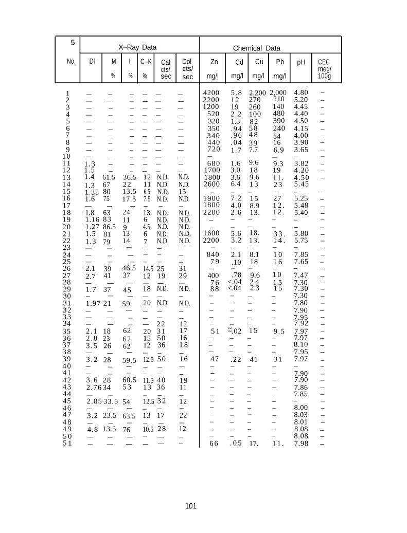
Chemical Data5
No.
X–Ray Data
DI M I C–K
% % %
Cal Dolcts/ cts/sec sec
Zn Cd Cu Pb pH
mg/l mg/l mg/l mg/l 100gmeg/CEC
12 —3 1404 4805 — 3206 5 87 340 4 8 848 — 440 169
10 — —1112 1.5 1913 1.4 N.D. N.D.14 2600 6.4 1 3 2 315 1.35 80 13.516 17.517 — — 1800 8.918 24 13. 1 2 .19 N.D. –20 86.5 9 N.D. N.D.2122 1 4 .23 — — –24 —25 — — 18 1 626 31 – –2728 — — 7 6 2 429 1.7 N.D. 8 8 2 3 1 5 7.3030 — —313233 — — —34 — — 12 –35 ~~36 23 5037 62 1238 — —39 1640 – –41 —42 28 60.5 –434445 12 –46 –4 74 84 9 125 0 –5 1
4200 5.8 2,200 2,000 4.80 –— — — — — —— — — — — 2200 12 270 210 5.20 –— — — — — — 1200 19 260 4.45 –— — — — — — 520 2.2 100 4.40 –— — — — — 1.3 82 390 4.50 –— — — — — — 350 .94 240 4.15 –— — — — — — .96 4.00 –
.04 39 3.90 –— — — — —— — — — — — 720 1.7 7.7 6.9 3.65 –— — — — — — — — — –
— — — — —1.3 680 1.6 9.6 9.3 3.82 –— — — — — 1700 3.0 18 4.20 –
61.5 36.5 12 1800 3.6 9.6 11. 4.50 –1.3 67 22 11 N.D. N.D. 5.45
6.5 N.D. 15 – – – – – –1.6 75 7.5 N.D. N.D. 1900 7.2 15 27 5.25 –— — — — 4.0 1 2 . 5.48 –1.8 63 13 N.D. N.D. 2200 2.6 5.40 –1.16 83 11 6 N.D. – – – – –1.27 4.5 – – – – – –
1600 5.6 18. 3 3 . 5.80 –1.5 81 13 6 N.D. N.D.1.3 79 14 7 N.D. N.D. 2200 3.2 13. 5.75 –— — — — – – – – –— — — — — 840 2.1 8.1 1 0 7.85 –— — — — 7 9 .10 7.65 –2.1 39 46.5 14.5 25 – – – –2.7 41 37 12 19 29 400 .78 9.6 1 0 7.47 –— — — — <.04 1 5 7.30 –
37 45 18 N.D. <.04 –– — — — – – – – 7.30 –
–1.97 21 59 20 N.D. N.D. – – – 7.80 –— — — — — — – – – – 7.90 –
— — — – – – – 7.95 –— — 22 – – – 7.92 –2 . 1 18 62 20 3 1 17 5 1 .02 1 5 9.5 7.97 –2 . 8 62 15 16 – – – – 7.97 –
8.103 . 5 26 36 1 8 – – – – –— — — — – – – – 7.95 –
3 . 2 28 59.5 12.5 50 47 .22 41 3 1 7.97 –— — — — — — – – – –— — — — — – – – – 7.90 –3 . 6 11.5 40 19 – – – 7.90 –2.76 34 5 3 13 36 11 – – – – 7.86 –— — — — — — – – – – 7.85 –2.85 33.5 54 12.5 3 2 – – – – –— — — — — — – – – 8.00 –3.2 23.5 63.5 13 17 22 – – – – 8.03 –— — — — — — – – – – 8.01 –4.8 13.5 76 10.5 28 – – – – 8.08 –— — — — — — – – – 8.08 –— — — — — — 6 6 . 0 5 17. 1 1 . 7.98 –
101
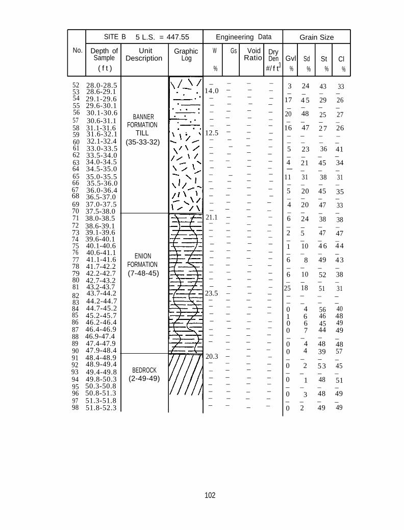
SITE B 5 L.S. = 447.55 Engineering Data Grain Size
No. Depth of Unit Graphic W Gs Void DrySample Description Log Ratio Den Gvl Sd St Cl
( f t ) % #/ f t3 % % % %
52 28.0-28.553 28.6-29.1 14.054 29.1-29.6
– – – 3 24 43 33
1755 29.6-30.1
––
– – – –– –
56 30.1-30.6
– – – – 4 5 29 26
57 30.6-31.1
– ––
– – – – –
58 31.1-31.6
20– – – – 48 25 27
59 31.6-32.1 12.5
–– –
–– ––
60 32.1-32.4
16 47–
– – – 27 26
61 33.0-33.5
–– – – – – – –
62 33.5-34.0
–– – –– – ––
63 34.0-34.5
– – – – 5 23 36 41
64 34.5-35.0
– – – –– – – –
65 35.0-35.5
– – – – 4 21 45 34
3166 35.5-36.0
– — –– – – – –
67 36.0-36.4
– – – – 11 31 38
68 36.5-37.0
– – – – –– – –
–69 37.0-37.5
– 5 20 45– – – 35
70 37.5-38.0
– – –– – – –
71 38.0-38.5 21.1
4 20 47 33– – –
72 38.6-39.1
– – ––
– – ––
73 39.1-39.6
–6– – – 24 38 38
74 39.6-40.1
– – – –– – ––
75 40.1-40.6
– – – – 2 5 47 47
1 4 6 4476
1040.6-41.1
––
– – – – – –
77 41.1-41.6
– – – –
78
– – – – – –– –
41.7-42.279 42.2-42.7
– 6– – 8 49– 43
80 42.7-43.2
– – – – – – – –
–81 43.2-43.7
– – – 6 10 52 38–
25 18 51 3182 43.7-44.2 23.5
–– – – – –
83 44.2-44.7
–– – –
84 44.7-45.2
–– – – – –– –
85 45.2-45.7
– – – – – – – –
86 46.2-46.4
– – – – 0 4 56 40
87 46.4-46.9
– – – –1 6 46 48
088 46.9-47.4
– – – – 0 6 45 49
89 47.4-47.9
– – – – 7 44 49
90 47.9-48.4
– – – – – – – –
91 48.4-48.9
–
20.3
– – – 0 4 48 48
92 48.9-49.4
– – – 0 4 39 57
93 49.4-49.8
– – – – – – –
94 49.8-50.3
– – – – 0 2 53 45
95 50.3-50.8
– – – – – – – –
96 50.8-51.3
– – – – 0 1 48 51
97 51.3-51.8
– – – – – – – –
98 51.8-52.3
BANNERFORMATION
TILL(35-33-32)
ENIONFORMATION(7-48-45)
BEDROCK(2-49-49)
– – – – 0 3 48 49– – – – – – – –– – – – 0 2 49 49
102
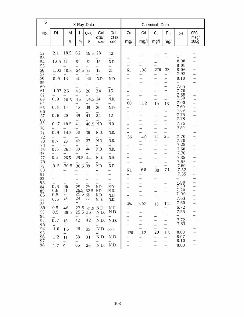
Chemical Data
– – – – – –– – – – – –– – – – 8.08 –– – – – 8.08 –61 .08 270 33 8.06 –– – – – 7.92 –– – – – 8.10 –– – – – – –– – – – 7.65 –– – – – 7.70 –– – – – 7.65 –– – – – 7.50 –60 . 1 2 15 13 7.00 –– – – – 7.60 –– – – – 7.69 –– – – – 7.75 –– – – – 7.78 –– – – – 7.75 –– – – – 7.80 –– – – – – –86 . 4 0 24 21 7.70 –– – – – 7.70 –– – – – 7.25 –– – – – 7.60 –– – – – 7.70 –– – – – 7.35 –– – – – 7.55 –– – – – 7.60 –6 1 . 6 8 38 7 1 7.52 –– – – – 7.55 –– – – – – –– – – – 7.80 –– – – – 7.20 –– – – – 7.70 –– – – – 7 .90 –– – – – 7.63 –36. <.02 15 1 4 7.60 –– – – – 6.72 –– – – – 7.56 –– – – – – –– – – – 7.72 –– – – – 7.83 –– – – – – –120. . 1 2
–20 1 3 8.00 –
– – – 8.07 –– – – – 8.10 –– – – – 8.00 –
–
2.1 18.5 6 2 19.5 28 12– – – – – –1.05 17 51 32 15 N.D.– – – – – –1.03 10.5 54.5 35 15 21– – – – – –0 . 9 13 51 36 N.D. N.D.– – – – – –– – – – – –1.07 2 6 4 5 28 34 15
– –0 . 9 20.5 4 5 34.5 24 N.D.– – – – – –0 . 8 15 46 39 20 N.D.– – – – – –0 . 6 20 39 41 24 12– – – – – –0 . 7 18.5 41 40.5 N.D. N.D.– – – – – –0 . 9 14.5 50 36 N.D. N.D.– – – – – –0 .7 23 40 37 N.D. N.D.– – – – – –0 . 5 26.5 30 44 N.D. N.D.– – – – – –0.5 26.5 29.5 44 N.D. N.D.– – – – – –0 . 5 30.5 30.5 39 N.D. N.D.
– – – – –– – – – – –– – – – – –– – – – – –
0.5 36 25.5 38 N.D. N.D.0 .5 46 24 30 N.D. N.D.– – – – – –0.5 4 6 23.5 31.5 N.D. N.D.0.5 38.5 25.5 36 N.D. N.D.– – – – – –0 . 7 16 42 4 2 N.D. N.D.– – – – – –1.0 1 6 49 35 N.D. 3 0– – – – – –1.2 11 58 31
– –N.D. N.D.
– – – –1.7 9 65 26 N.D. N.D.
0 . 6 46 25 29 N.D. N.D.
– – – –
0.6 41 26.5 32.5 N.D. N.D.
5X-Ray Data
M I C–KNo. DI
% % % seccts/Cal
seccts/Dol Zn Cd Cu Pb pH
mg/l mg/l mg/l mg/l 100gmeg/CEC
5253545556575859606162636465666768697071727374757677787980818283848586878889909192939495969798
103
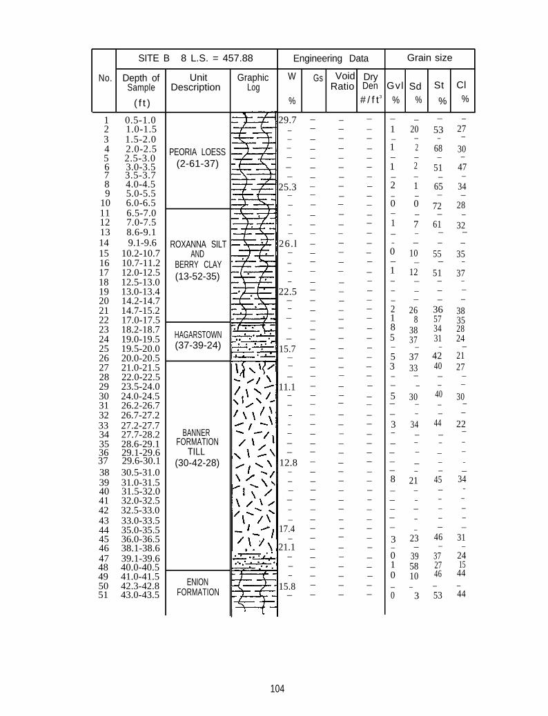
Grain size
No. Depth of W Gs Void DrySample Ratio Den Gvl Sd St Cl
( f t )
SITE B 8 L.S. = 457.88 Engineering Data
UnitDescription
GraphicLog
% # / f t3 % % % %
1 0.5-1.02 1.0-1.53 1.5-2.04 2.0-2.55 2.5-3.06 3.0-3.57 3.5-3.78 4.0-4.59 5.0-5.5
10 6.0-6.511 6.5-7.012 7.0-7.513 8.6-9.114 9.1-9.6
38 30.5-31.039 31.0-31.540 31.5-32.041 32.0-32.542 32.5-33.043 33.0-33.544 35.0-35.545 36.0-36.546 38.1-38.647 39.1-39.648 40.0-40.549 41.0-41.550 42.3-42.851 43.0-43.5
33 27.2-27.734 27.7-28.235 28.6-29.1
15 10.2-10.716 10.7-11.217 12.0-12.518 12.5-13.019 13.0-13.420 14.2-14.721 14.7-15.222 17.0-17.523 18.2-18.724 19.0-19.525 19.5-20.026 20.0-20.527 21.0-21.528 22.0-22.529 23.5-24.030 24.0-24.531 26.2-26.732 26.7-27.2
36 29.1-29.637 29.6-30.1
PEORIA LOESS(2-61-37)
ROXANNA SILTAND
BERRY CLAY(13-52-35)
HAGARSTOWN(37-39-24)
BANNERFORMATION
TILL(30-42-28)
ENIONFORMATION
29.7 – – – – – – –– – – – 1 20 53 27– – – – – – – –– – – – 1 2 68 30– – – – – – – –– – – – 1 2 51 47– – – – – – – –
– – – 2 1 65 34– – – – – – – –– – – – 0 0 72 28– – – – – – – –– – – 1 7 61– 32– – – – – – – –
– – – – – – –– – – – 0 55 35– – – – – – – –– – – – 1 51 37
10
12
25.3
26.l
– – – – – – – –22.5 – – – – – – –
– – – – – – – –– – – – 2 26 36– – – 1– 8 57
– – 8– – 38 34– – – 5– 37 31
– – – – – – –– – – – 5 37 42 21– – – 3– 33 40– – – – – – – –
– – – – – – –– – – 5– 30 40
– – – – – – – –– – – – – – – –– – – – 3 34
38352824
27
30
15.7
11.1
44 22– – – – – – – –– – – – – – – –– – – – – – – –
12.8 – – – – – – –– – – – – – – –
8– – – – 21 45 34– – – – – – – –– – – – – – – –– – – – – – – –
– – – –17.4 – – – –
––
––
– ––
– – – 3 46 31– 2321.1 – – – – – – –
– – – 0– 39 37 24– – 1– – 58 27 15– – – – 0 10 46 44
15.8 – – – – – – –– – – 0 3 53 44–
104
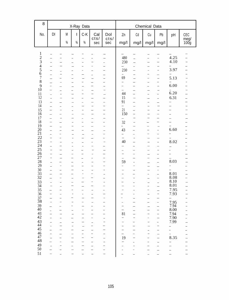
8X-Ray Data Chemical Data
No. DI M I C-K Cal Dol Zn Cd Cu Pb pH CECc ts / c ts / meg/
% % % sec sec mg/l mg/l mg/l mg/l 100g
1 – – – – – –2 – – – – – –3 – – – – – –4 – – – – – –5 – – – – – –6 – – – – – –7 – – – – – –8 – – – – – –9 – – – – – –
10 – – – – – –11 – – – – – –12 – – – – – –13 – – – – – –14 – – – – – –15 – – – – – –16 – – – – – –17 – – – – – –18 – – – – – –19 – – – – – –20 – – – – – –21 – – – – – –22 – – – – – –23 – – – – – –24 – – – – – –25 – – – – – –26 – – – – – –27 – – – – – –28 – – – – – –29 – – – – – –30 – – – – – –31 – – – – – –32 – – – – – –33 – – – – – –34 – – – – – –35 – – – – – –36 – – – – – –37 – – – – – –38 – – – – – –39 – – – – – –40 – – – – – –41 – – – – – –42 – – – – – –43 – – – – – –44 – – – – – –45 – – – – – –46 – – – – – –47 – – – – – –48 – – – – – –49 – – – – – –50 – – – – – –51 – – – – – –
– – – – – –480 – – – 4.25 –230 – – – 4.10 –– – – – – –230 – – – 3.97 –– – – – – –69 – – – 5.13 –– – – – – –– – – – 6.00 –– – – – – –44 – – – 6.20 –15 – – – 6.31 –91 – – – – –– – – – – –21 – – – – –150 – – – – –– – – – – –32 – – – – –– – – – – –43 – – – 6.60 –– – – – – –– – – – – –40 – – – 8.02 –– – – – – –– – – – – –– – – – – –– – – – – –59 – – – 8.03 –– – – – – –– – – – – –– – – – 8.01 –– – – – 8.08 –– – – – 8.10 –– – – – 8.01 –– – – – 7.95 –– – – – 7.93 –– – – – – –– – – – 7.95 –– – – – 7.94 –– – – – 8.00 –81 – – – 7.94 –– – – – 7.90 –– – – – 7.99 –– – – – – –– – – – – –– – – – – –19 – – – 8.35 –– – – – – –– – – – – –– – – – – –– – – – – –
105
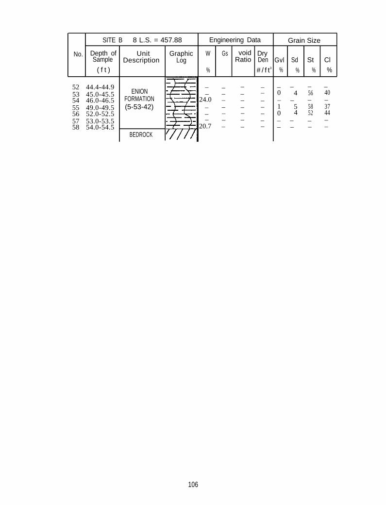
GraphicLog
W Gs void DryRatio Den Gvl Sd St Cl
% # / f t3 % % % %( f t )
SampleDepth of
SITE B 8 L.S. = 457.88 Engineering Data
No.Description
Unit
52 44.4-44.953 45.0-45.554 46.0-46.555 49.0-49.556 52.0-52.557 53.0-53.558 54.0-54.5
ENIONFORMATION(5-53-42)
– – – –– – – –
24.0 – – –– – – –– – – –– – – –
20.7 – – –
Grain Size
– – – –0 4 56 40– – – –1 5 58 370 4 52 44– – – –– – – –
BEDROCK
106
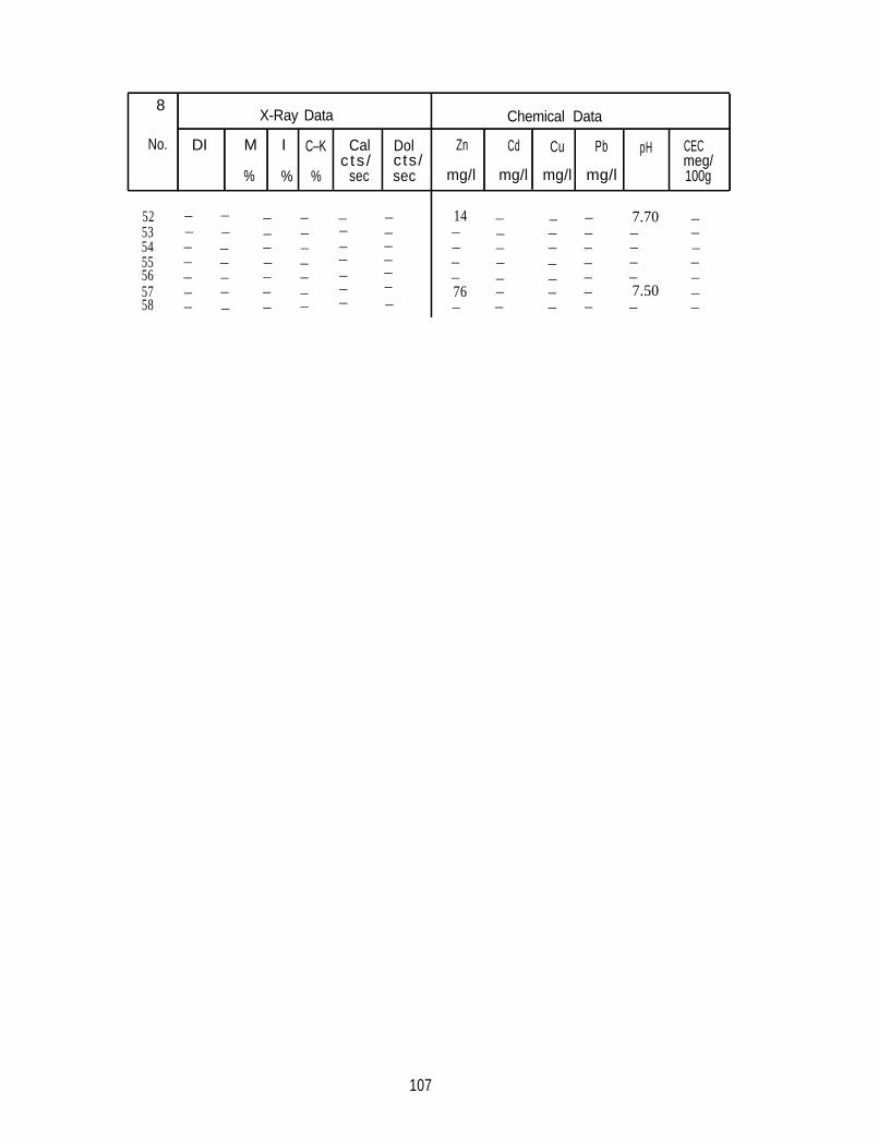
8
No.
X-Ray Data
DI M I C–K
% % %
Cal Dolc ts / cts/
sec sec
Chemical Data
Zn Cd Cu Pb pH
mg/l mg/l mg/l mg/l
CECmeg/100g
– –52 – –53 – – – – – –54 – – – –
– –
– –55 – – – – – –56 – – – – – –57 – – – – – –58 – – – – – –
14 – – – 7.70 –– – – – – –– – – – – –– – – – – –– – – – – –76 – – – 7.50 –– – – – – –
107
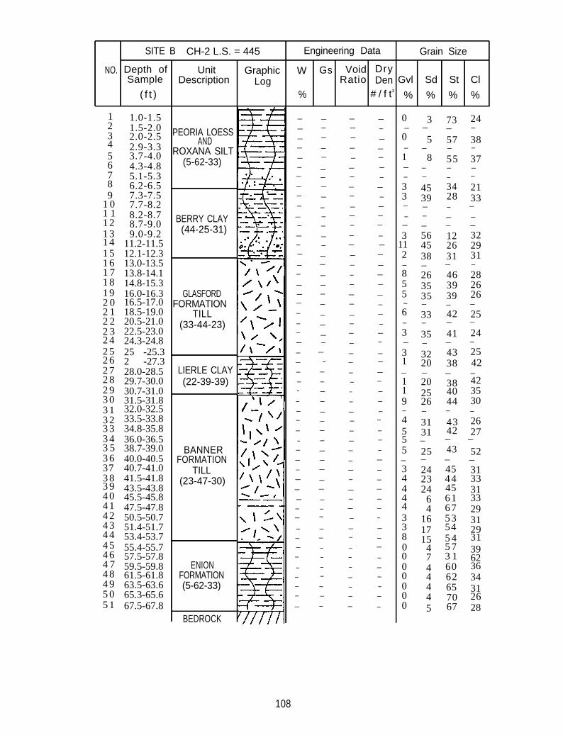
NO. Depth of W Gs Void DrySample Ratio Den
( f t )
SITE B CH-2 L.S. = 445 Engineering Data
Unit GraphicDescription Log
Grain Size
Gvl Sd St Cl
% # / f t3% % % %
1 1.0-1.52 1.5-2.03 2.0-2.54 2.9-3.35 3.7-4.06 4.3-4.87 5.1-5.38 6.2-6.59 7.3-7.5
1 0 7.7-8.21 1 8.2-8.71 2 8.7-9.01 3 9.0-9.21 4 11.2-11.51 5 12.1-12.31 6 13.0-13.51 7 13.8-14.11 8 14.8-15.31 9 16.0-16.32 0 16.5-17.02 1 18.5-19.02 2 20.5-21.02 3 22.5-23.02 4 24.3-24.82 5 25 -25.32 6 2 -27.32 7 28.0-28.52 8 29.7-30.02 9 30.7-31.03 0 31.5-31.83 1 32.0-32.53 2 33.5-33.83 3 34.8-35.83 4 36.0-36.53 5 38.7-39.03 6 40.0-40.537 40.7-41.03 8 41.5-41.83 9 43.5-43.84 0 45.5-45.84 1 47.5-47.84 2 50.5-50.74 3 51.4-51.74 4 53.4-53.74 54 6
55.4-55.757.5-57.8
4 74 8
59.5-59.861.5-61.8
4 9 63.5-63.65 0 65.3-65.65 1 67.5-67.8
BEDROCK
ENIONFORMATION(5-62-33)
BANNER
TILL(23-47-30)
LIERLE CLAY(22-39-39)
GLASFORDFORMATION
TILL(33-44-23)
BERRY CLAY(44-25-31)
PEORIA LOESSAND
ROXANA SILT(5-62-33)
FORMATION
– – – –– – – –– – – –– – – –– – – –– – – –– – – –– – – –– – – –– – – –– – – –– – – –– – – –– – – –– – – –– – – –– – – –– – – –– – – –– – – –– – – –– – – –– – – –– – – –– – – –– – – –– – – –– – ––– – – –– – – –– – – –– – – –– – – –– – – –– – – –– – – –– – – –– – – –– – – –– – – –– – – –– – – –– – – –– – – –– – – –– – – –– – – –– – – –– – – –– – – –– – – –
0 3 73 24– – – –
0 5 57 38– – – –1 8 55 37– – – –– – – –3 45 343 39
2128 33
– – – –– – – –– – – –3 56
11 45 292 38– – – –8 265 355 35– – – –6 33
122631
463939
42– – – –3 41– – – –3 43 251 38 42– – – –1 38 421 40 359 44
32
31
282626
35
3220
25
24
202526 30
– – – –4 315 31
4342
2627
5 – – –5 43 52– – – –3 45 314 23 44 334 45 314 61 334 67 293 53 313 54 298 5 4 310 5 7 390 7 3 1 620 60 360 62 340 4 65 310 70 260 28
25
24
2464
161715
4
44
45 67
108
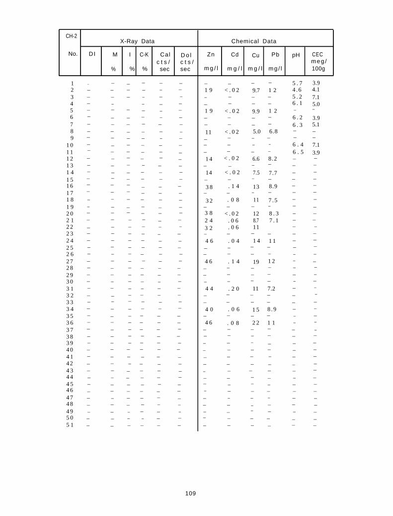
No. I C-K Cal D o l Zn Cd Cu Pb pH CECc t s / c t s / m e g /
% % sec sec
X-Ray DataCH-2
Chemical Data
DI M
% m g / l m g / l m g / l mg / l 100g
1 – – – – – –2 – – – – – –3 – – – – – –4 – – – – –5 – – – – – –6 – – – – – –7 – – – – – –8 – – – – – –9 – – – – – –
1 0 – – – – – –1 1 – – – – – –1 2 – – – – – –1 3 – – – – – –1 4 – – – – – –1 5 – – – – – –1 6 – – – – – –1 7 – – – – – –1 8 – – – – – –1 9 – – – – – –2 0 – – – – – –2 1 – – – – – –2 2 – – – – – –2 3 – – – – – –2 4 – – – – – –2 5 – – – – – –2 6 – – – – – –2 7 – – – – – –2 8 – – – – – –2 9 – – – – – –3 0 – – – – – –3 1 – – – – – –3 2 – – – – – –3 3 – – – – – –3 4 – – – – – –
3 5 – – – – – –3 6 – – – – – –3 7 – – – – – –3 8 – – – – – –3 9 – – – – – –4 0 – – – – – –4 1 – – – – – –42 – – – – – –4 3 – – – – – –4 4 – – – – – –4 5 – – – – – –4 6 – – – – – –4 7 – – – – – –4 8 – – – – – –4 9 – – – – – –5 0 – – – – – –5 1 – – – – – –
– – – – 5 . 7 3.94 . 6 4.1
– – – – 5 . 2– – – – 6 . 1
– –
– – – –– – – –
– –– – – – – –– – – –– – – –
– –– – – – – –
– –– – – – – –
– –– – – – – –
– –– – – – – –3 8 12 – –
– –– –
– – – – – –– –
– – – – – –– – – – – –4 6 . 1 4
1 9 < . 0 2 9.7
9.9
5.0< . 0 2
< . 0 21 9
11
1 2
6.8
1 2
6 . 46 . 5
6 . 26 . 3
7.15.0
3.95.1
7.13.9
1 4
14
3 8
3 2
2 43 2
4 6
< . 0 2
< . 0 2
. 1 4
. 0 8
< . 0 2. 0 6. 0 6
. 0 4
6.6
7.5
13
11
8.711
1 4
8.2
7.7
8.9
7 . 5
8 . 37 . 1
1 1
1 2 – –– – – – – –– – – – – –– – – – – –
7.2 –– – – – –– – – – –
8 . 9 –– – – – –
1 1
4 4
4 0
4 6 . 0 8
. 0 6
19
11
1 5
2 2
. 2 0 ––––
–– –
– – – – – –– – – – – –– – – – – –– – – – – –– – – – – –– – – – – –– – – – – –– – – – – –– – – – – –– – – – – –– – – – – –– – – – – –– – – – – –– – – – – –– – – – – –
109
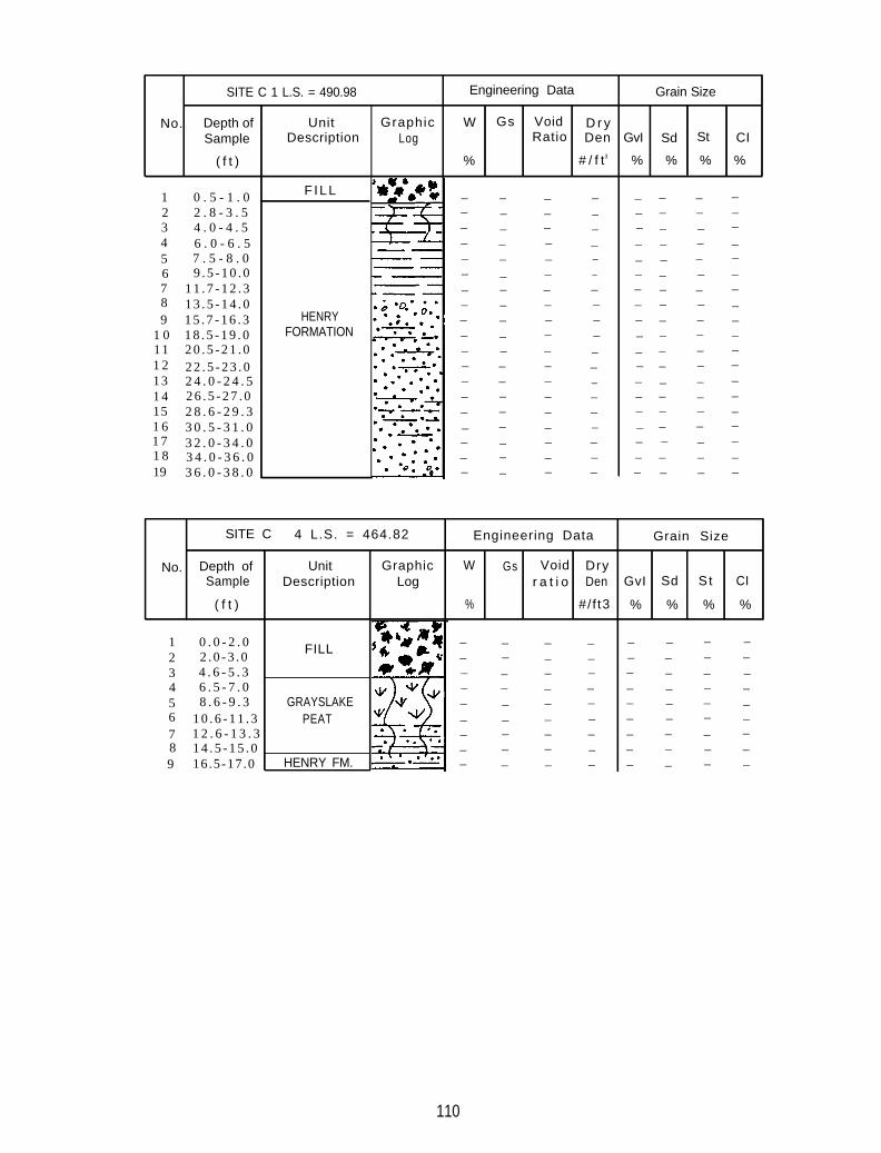
No. Depth of W Sample Description Ratio
( f t )
SITE C 1 L.S. = 490.98 Engineering Data Grain Size
Unit Graphic Gs Void D r yLog Den
% # / f t3
F ILL
GvI Sd St CI
% % % %
1 0 . 5 - 1 . 0 – – – – – – – –2 2 . 8 - 3 . 5 – – – – – – – –3 – – – – – – – –4 . 0 - 4 . 54 6 . 0 - 6 . 5 – – – – – – – –5 7 . 5 - 8 . 0 – – – – – – – –6 9 . 5 - 1 0 . 0 – – – – – – – –7 1 1 . 7 - 1 2 . 3 – – – – – – – –8 – – – – – – – –1 3 . 5 - 1 4 . 09 1 5 . 7 - 1 6 . 3 – – – – – – – –
1 0 – – – – – – –1 8 . 5 - 1 9 . 011 2 0 . 5 - 2 1 . 0 – – – – – – –1 2 2 2 . 5 - 2 3 . 0 – – – – – – –13 2 4 . 0 - 2 4 . 5 – – – – – –1 4 2 6 . 5 - 2 7 . 0 – – – – – – –15 2 8 . 6 - 2 9 . 3 – – – – – – –1 6 3 0 . 5 - 3 1 . 0 – – – – – – – –1 7 3 2 . 0 - 3 4 . 0 – – – – – – –1 8 3 4 . 0 - 3 6 . 0 – – – – – – –19 3 6 . 0 - 3 8 . 0
HENRYFORMATION –
––
– –––
––
– – – – – – – –
SITE C 4 L.S. = 464.82 Engineering Data
No. Depth of Unit Graphic W Gs Void DrySample Description Log r a t i o Den GvI Sd St CI
( f t )
Grain Size
% #/f t3 % % % %
1 0 . 0 - 2 . 0 – – – – – – – –2 2 . 0 - 3 . 0
FILL– – – – – – – –
3 4 . 6 - 5 . 3 – – – – – – – –4 6 . 5 - 7 . 0 – – – – – – – –5 8 . 6 - 9 . 3 GRAYSLAKE – – – – – – – –6 1 0 . 6 - 1 1 . 3 PEAT – – – – – – – –7 1 2 . 6 - 1 3 . 3 – – – – – – – –8 1 4 . 5 - 1 5 . 0 – – – – – – – –9 16.5-17 .0 HENRY FM. – – – – – – – –
110
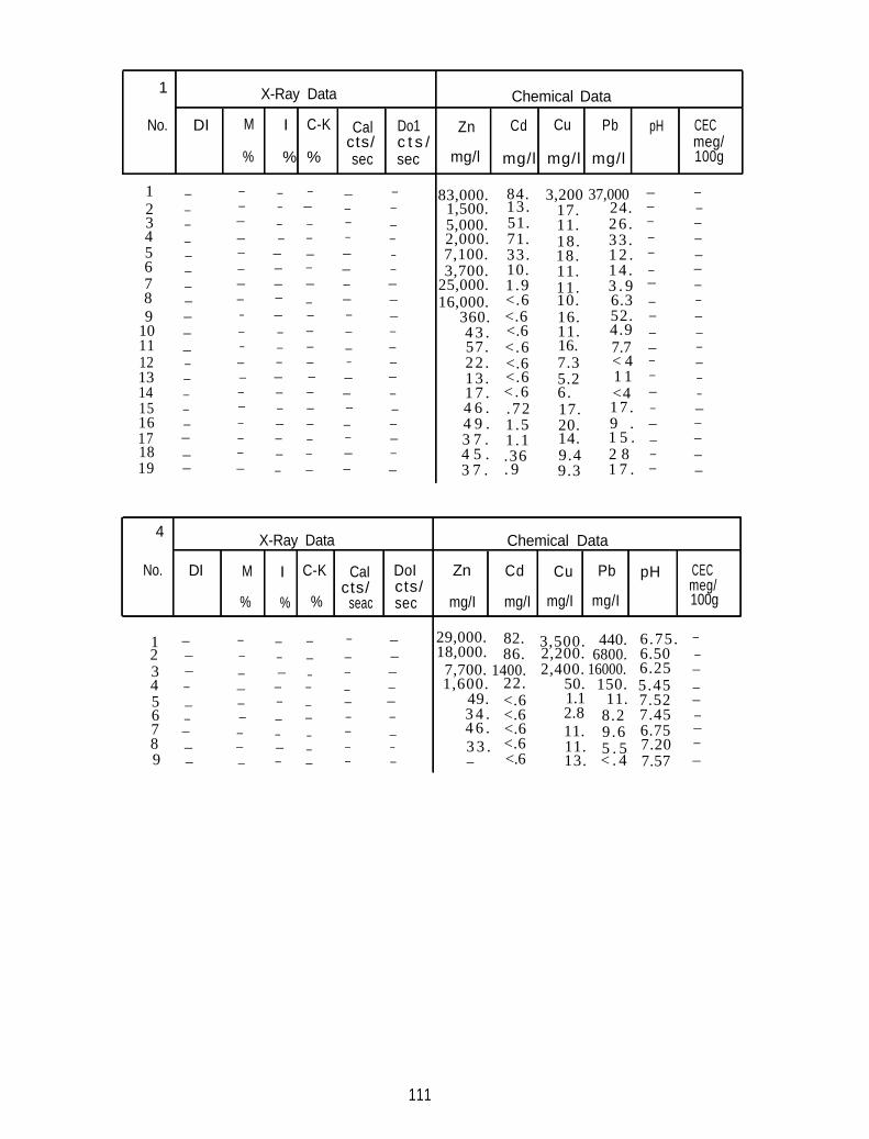
1 X-Ray Data Chemical Data
No. DI M I C-K Cal Do1 Zn Cd Cu Pb pH CECcts/ c t s / meg/
% % % sec sec mg/l mg/l mg/l mg/l 100g
1 – – – – – – 83,000.2 – – – – – – 1,500. 13. 24. –3 – – – – – – 5,000. 11. 26 . –4 – – – – – – 2,000. –5 – – – – – – 7,100. 18. 1 2 . –6 – – – – – – 3,700. 10. 11. –7 – – – – – – 25,000. –8 – – – – – – 16,000. 10. 6.3 – –9 – – – – – – 360. – –
10 – – – – – – 4 3 . <.6 11. 4.9 –11
–– – – – – – 57. <.6 16. 7.7 – –
12 – – – – – – 22 . 7.3 < 4 – –13
<.6– – – – – – 13 . <.6 1 1 –
145.2 –
– – – – – 1 7 . < .6 6. <4 – ––15 – – – – – – 4 6 . 17. 17 . –16 – – – – – –
–4 9 . 9 . – –
17 – – – – – 3 7 . 14. 1 5 . –18
–– – – – – – 4 5 . 2 8 –
19–
– – – – – 3 7 .
84. 3,200 37,000 – –
51.17.
–71. 18. 33 .
–
–33.
14 . –1 .9 11. 3 . 9
–
–<.6<.6 16. 52.
.721 .5 20.
–
1 .1.36 9.4
1 7 . –. 9 9.3– –
4X-Ray Data Chemical Data
No. DI M I C-K CaI DoI Zn Cd Cu Pb pH CECcts/ cts/ meg/
% % % seac sec mg/I mg/I mg/I mg/I 100g
1 – – – – – – 29,000. 82. 3,500. 440. 6.75. –2 – – – – – – 18,000. 86. 2,200. 6800. 6.50 –3 – – – – – – 7,700. 1400. 2,400. 16000. 6.25 –4 – – – – – – 1,600. 22. 50. 150. 5.45 –5 – – – – – – 49. <.6 1.1 11. 7.52 –6 – – – – – – 3 4 . <.6 2.8 8.2 7.45 –7 – – – – – – 4 6 . <.6 11. 9 .6 6.75 –8 – – – – – – 3 3 . <.6 11. 5 . 5 7.20 –9 – – – – – – 13. < . 4 –– <.6 7.57
111
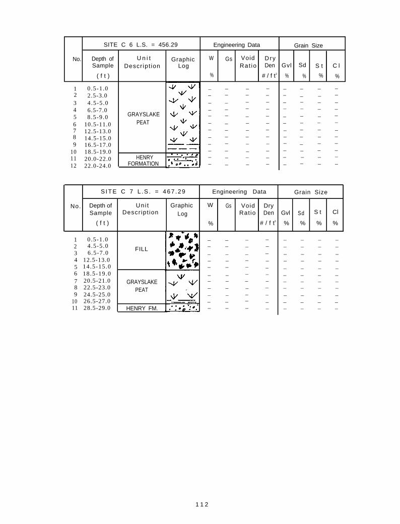
SITE C 6 L.S. = 456.29 Engineering Data Grain Size
No. Depth of U n i t Graphic W Gs Void DrySample Descr ipt ion Log Rat io Den Gvl Sd S t C l
( f t ) % # / f t3 % % % %
1 0.5-1 .0 – – – – – – – –2 2.5-3.0 – – – – – – – –3 4.5-5 .0 – – – – – – – –4 6.5-7.0 – – – – – – – –
8.5-9 .0 GRAYSLAKE5 – – – – – – – –
6 10.5-11.0 PEAT – – – – – – – –
7 12.5-13.0 – – – – – – – –8 14.5-15.0 – – – – – – – –9 16.5-17.0 – – – – – – – –
10 18.5-19.0 – – – – – – – –
11 20.0-22.0 HENRY – – – – – – – –
12 22.0-24.0 FORMATION – – – – – – – –
Grain Size
No. Depth of WSample Gvl Sd S t Cl
( f t )
– –– –
S I T E C 7 L . S . = 4 6 7 . 2 9 Engineering Data
1 0.5-1 .02 4.5-5 .0 – –3 6.5-7 .0
Uni tDescr ipt ion
Graphic
LogGs
%
Void DryRat io Den
# / f t3 % % % %
– – – –– – – –
– – – – – –4 12.5-13.0 – – – – – –5 14.5-15 .0 – – – – – –6 18.5-19 .0 – – – – – –7 20.5-21.0 – – – – – –
22.5-23.0 – – – – – –24.5-25.0 – – – – – –
10 26.5-27.0 – – – – – –– – – – –
– –– –
– –– –– –
– –– –
– –– –
– –
FILL
GRAYSLAKEPEAT
HENRY FM.
89
11 28.5-29.0 –
1 1 2
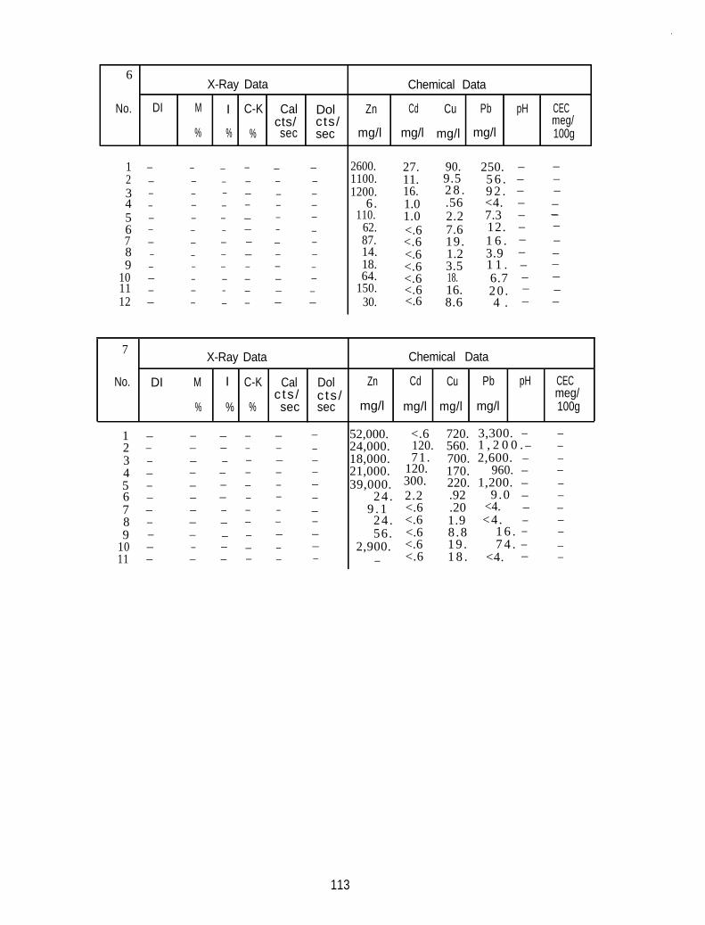
6
No.
X-Ray Data
DI M I C-K Cal Dolcts/ cts/
% % % sec sec
Chemical Data
Zn Cd Cu Pb pH CECmeg/
mg/l mg/l mg/l mg/l 100g
1 – – – – – –2 – – – – – –3 – – – – – –4 – – – – – –5 – – – – – –6 – – – – – –7 – – – – – –8 – – – – ––9 – – – – – –
10 – – – – – –11 – – – – – –12 – – – – – –
7X-Ray Data Chemical Data
No. DI M I C-K Cal Dol Zn Cd Cu Pb pH CECc ts / c ts / meg/
% % % sec sec mg/l mg/l mg/l mg/l 100g
2600. 27. 90. 250. – –1100. 11. 5 6 . – –1200. 16.
9.52 8 . 9 2 . – –
6. 1.0 .56 <4. – –110. 1.0 7.3 – ––
62. <.6 7.6 12. – –87. <.6
2.2
19. – –14. <.6
1 6 .1.2 3.9 – –
18. <.6 1 1 . – –64.
3.5<.6 – —
150.18. 6.7
<.6 16. 20 . – –30. <.6 8.6 4 . – –
1 – – – – – –2 – – – – – –3 – – – – – –4 – – – – – –5 – – – – – –6 – – – – – –7 – – – – – –8 – – – – – –9 – – – – – –
10 – – – – – –11 – – – – – –
52,000. 3,300. –24,000. 560. 1 , 2 0 0 . –18,000.21,000. 960.39,000. 300.
9 . 1
56. 1 6 . –2,900.
71.– –120. 170.
2,600. –
–220. 1,200. ––2.2 .92 9 .0 ––<.6 .20 <4. ––<.6 1.9 <4 . ––
<.68 .8<.619 . 7 4 . – –
<.6 1 8 . –
<.6 720. –120.
700. –
–
24 .
24 .
– <4. –
113


