
Rome, 13-16/11/2018
Remote Sensing of Soil Moisture
Sebastian Hahn, Mariette Vreugdenhil, Bernhard Bauer-Marschallinger, Wolfgang Wagner
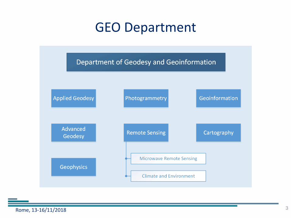
Department of Geodesy and Geoinformation (GEO), TU Wien http://www.geo.tuwien.ac.at/
Rome, 13-16/11/2018
Topics
• Introduction
• Microwave Remote Sensing
• Spaceborne Microwave Instruments
• Sampling Requirements
• Retrieval Approaches
• Summary
2
Rome, 13-16/11/2018
GEO Department
3
Rome, 13-16/11/2018
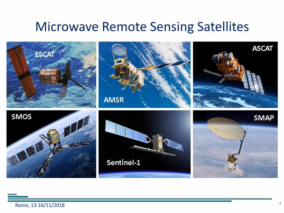
Microwave Remote Sensing Satellites
4
Rome, 13-16/11/2018
Microwave Remote Sensing
5
Rome, 13-16/11/2018
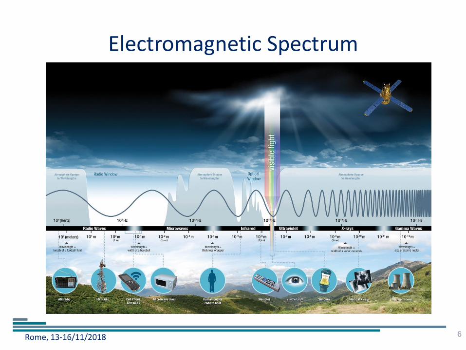
Electromagnetic Spectrum
6
Image credit: NASA
Rome, 13-16/11/2018
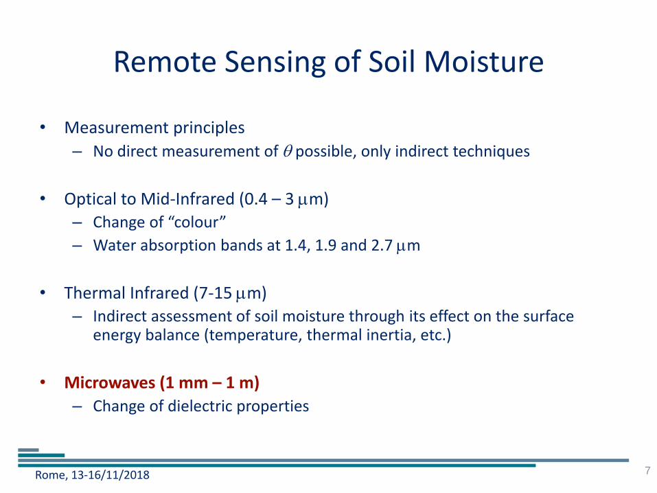
Remote Sensing of Soil Moisture
• Measurement principles
– No direct measurement of possible, only indirect techniques
• Optical to Mid-Infrared (0.4 – 3 m)
– Change of “colour”
– Water absorption bands at 1.4, 1.9 and 2.7 m
• Thermal Infrared (7-15 m)
– Indirect assessment of soil moisture through its effect on the surface energy balance (temperature, thermal inertia, etc.)
• Microwaves (1 mm – 1 m)
– Change of dielectric properties
7
Rome, 13-16/11/2018
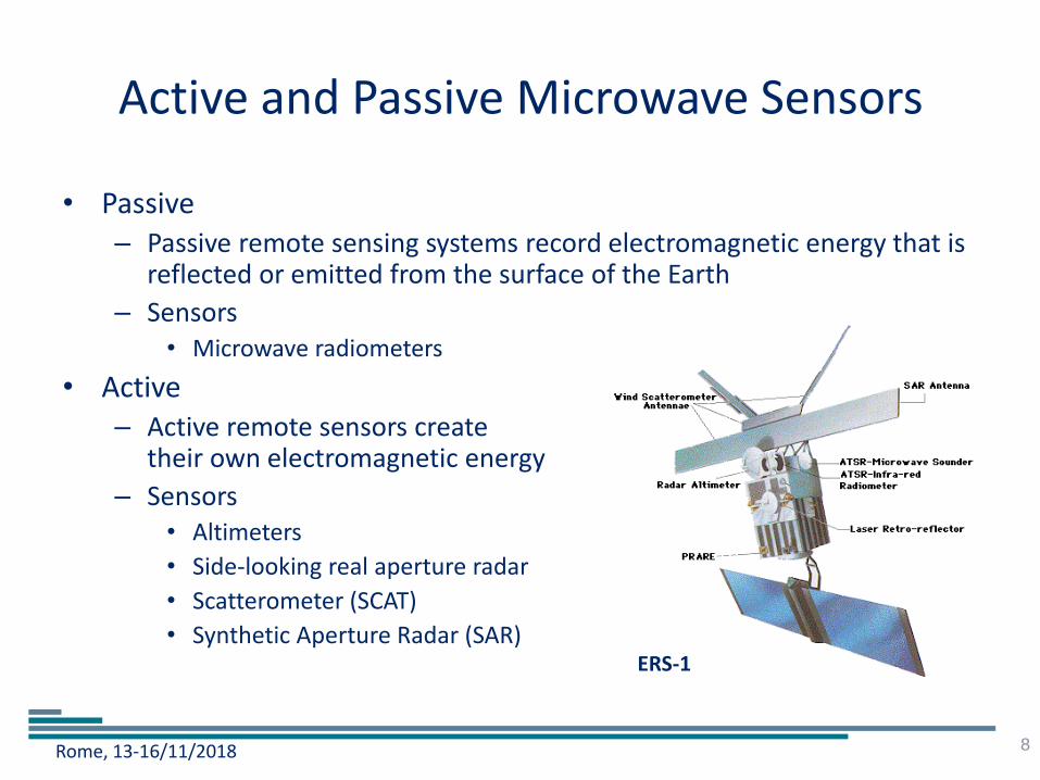
Active and Passive Microwave Sensors
• Passive – Passive remote sensing systems record electromagnetic energy that is
reflected or emitted from the surface of the Earth
– Sensors • Microwave radiometers
• Active – Active remote sensors create
their own electromagnetic energy
– Sensors • Altimeters
• Side-looking real aperture radar
• Scatterometer (SCAT)
• Synthetic Aperture Radar (SAR)
8
ERS-1
Rome, 13-16/11/2018
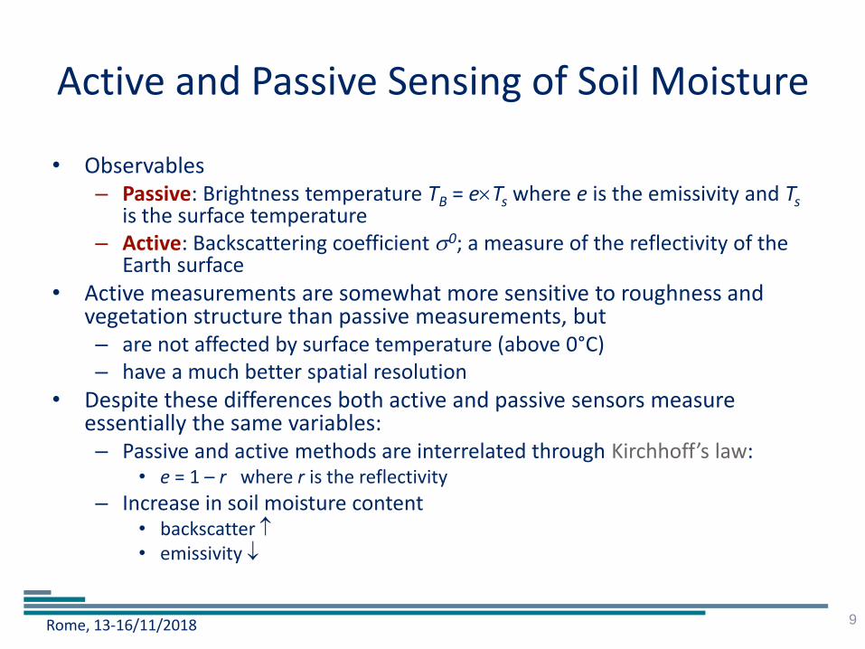
Active and Passive Sensing of Soil Moisture
• Observables – Passive: Brightness temperature TB = eTs where e is the emissivity and Ts
is the surface temperature – Active: Backscattering coefficient 0; a measure of the reflectivity of the
Earth surface
• Active measurements are somewhat more sensitive to roughness and vegetation structure than passive measurements, but – are not affected by surface temperature (above 0°C) – have a much better spatial resolution
• Despite these differences both active and passive sensors measure essentially the same variables: – Passive and active methods are interrelated through Kirchhoff’s law:
• e = 1 – r where r is the reflectivity
– Increase in soil moisture content • backscatter • emissivity
9
Rome, 13-16/11/2018
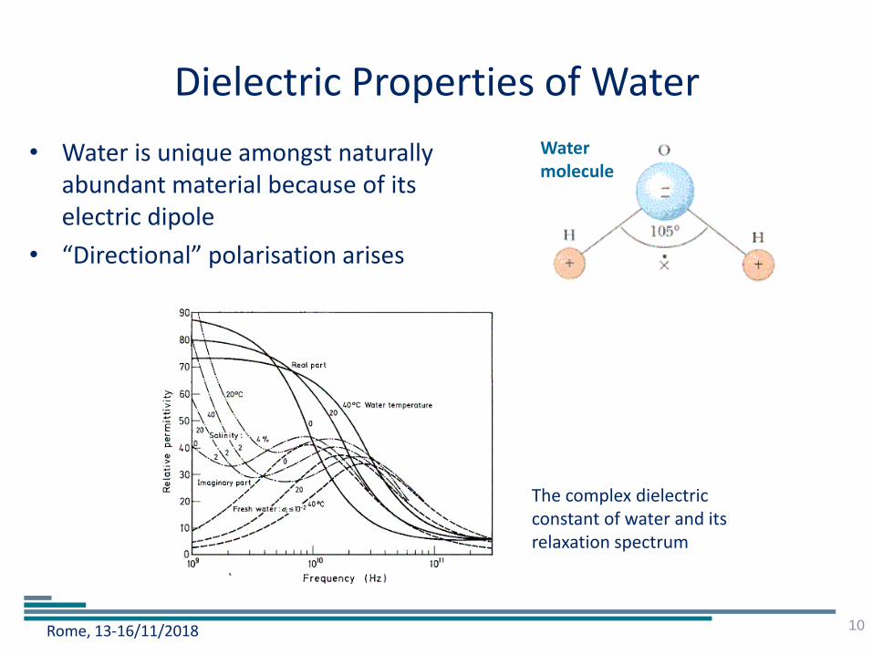
Dielectric Properties of Water
• Water is unique amongst naturally abundant material because of its electric dipole
• “Directional” polarisation arises
10
Water molecule
The complex dielectric constant of water and its relaxation spectrum
Rome, 13-16/11/2018
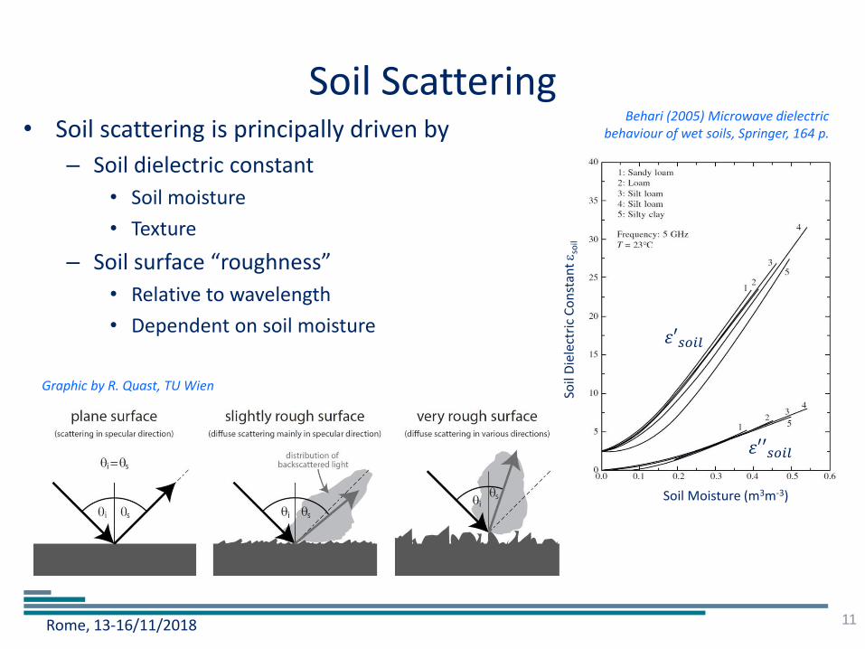
Soil Scattering • Soil scattering is principally driven by
– Soil dielectric constant
• Soil moisture
• Texture
– Soil surface “roughness”
• Relative to wavelength
• Dependent on soil moisture
11
Graphic by R. Quast, TU Wien
Soil Moisture (m3m-3)
Soil
Die
lect
ric
Co
nst
ant s
oil
Behari (2005) Microwave dielectric behaviour of wet soils, Springer, 164 p.
휀′𝑠𝑜𝑖𝑙
휀′′𝑠𝑜𝑖𝑙
Rome, 13-16/11/2018
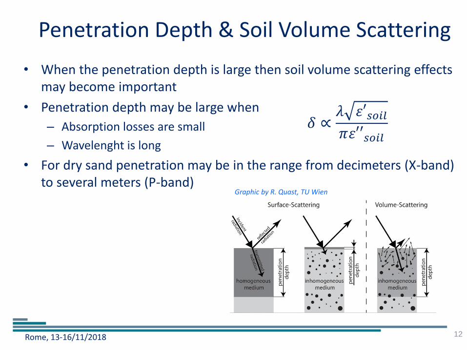
Penetration Depth & Soil Volume Scattering
• When the penetration depth is large then soil volume scattering effects may become important
• Penetration depth may be large when
– Absorption losses are small
– Wavelenght is long
• For dry sand penetration may be in the range from decimeters (X-band) to several meters (P-band)
12
Graphic by R. Quast, TU Wien
𝛿 ∝𝜆 휀′𝑠𝑜𝑖𝑙𝜋휀′′𝑠𝑜𝑖𝑙
Rome, 13-16/11/2018
Spaceborne Microwave Instruments
13
Rome, 13-16/11/2018
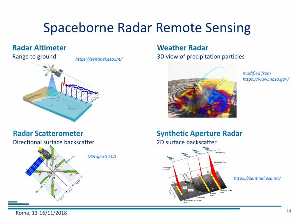
Spaceborne Radar Remote Sensing
14
Radar Altimeter Range to ground https://sentinel.esa.int/
Weather Radar 3D view of precipitation particles
Radar Scatterometer Directional surface backscatter
Synthetic Aperture Radar 2D surface backscatter
https://sentinel.esa.int/
modified from https://www.nasa.gov/
Metop-SG SCA
Rome, 13-16/11/2018
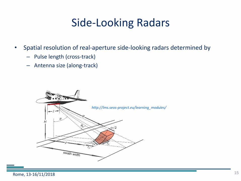
Side-Looking Radars
• Spatial resolution of real-aperture side-looking radars determined by
– Pulse length (cross-track)
– Antenna size (along-track)
15
http://lms.seos-project.eu/learning_modules/
Rome, 13-16/11/2018
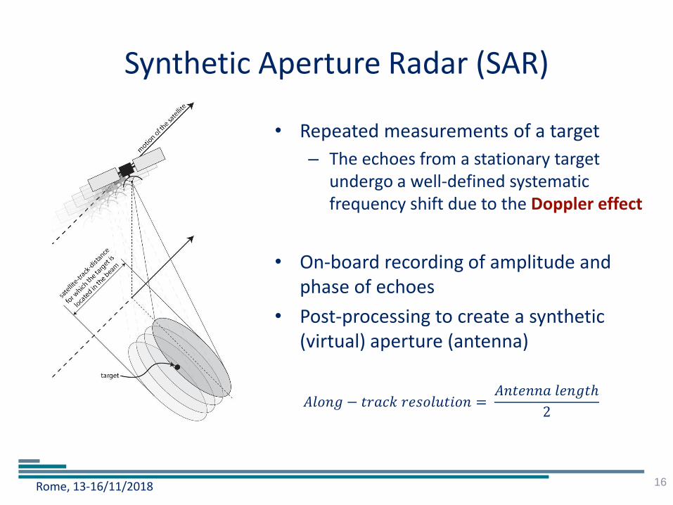
Synthetic Aperture Radar (SAR)
• Repeated measurements of a target
– The echoes from a stationary target undergo a well-defined systematic frequency shift due to the Doppler effect
• On-board recording of amplitude and phase of echoes
• Post-processing to create a synthetic (virtual) aperture (antenna)
16
𝐴𝑙𝑜𝑛𝑔 − 𝑡𝑟𝑎𝑐𝑘 𝑟𝑒𝑠𝑜𝑙𝑢𝑡𝑖𝑜𝑛 = 𝐴𝑛𝑡𝑒𝑛𝑛𝑎 𝑙𝑒𝑛𝑔𝑡ℎ
2
Rome, 13-16/11/2018
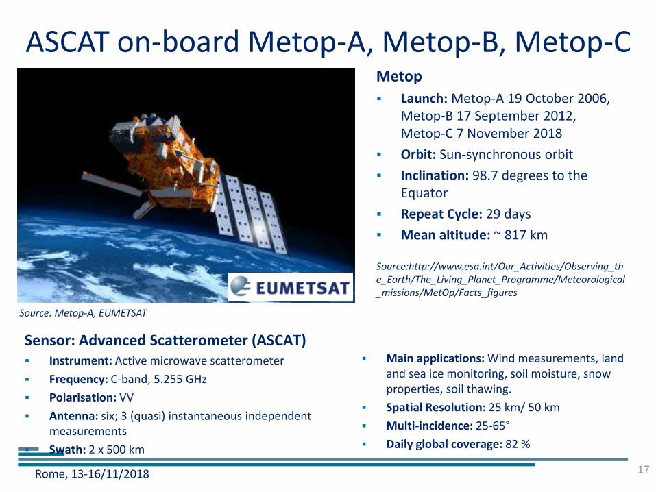
ASCAT on-board Metop-A, Metop-B, Metop-C
17
Metop
Launch: Metop-A 19 October 2006, Metop-B 17 September 2012, Metop-C 7 November 2018
Orbit: Sun-synchronous orbit
Inclination: 98.7 degrees to the Equator
Repeat Cycle: 29 days
Mean altitude: ~ 817 km
Source: Metop-A, EUMETSAT
Source:http://www.esa.int/Our_Activities/Observing_the_Earth/The_Living_Planet_Programme/Meteorological_missions/MetOp/Facts_figures
Sensor: Advanced Scatterometer (ASCAT) Instrument: Active microwave scatterometer
Frequency: C-band, 5.255 GHz
Polarisation: VV
Antenna: six; 3 (quasi) instantaneous independent measurements
Swath: 2 x 500 km
Main applications: Wind measurements, land and sea ice monitoring, soil moisture, snow properties, soil thawing.
Spatial Resolution: 25 km/ 50 km
Multi-incidence: 25-65°
Daily global coverage: 82 %
Rome, 13-16/11/2018
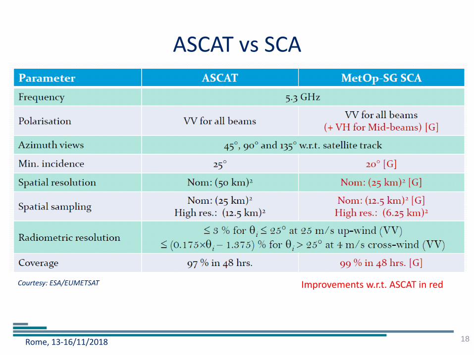
ASCAT vs SCA
18
Improvements w.r.t. ASCAT in red Courtesy: ESA/EUMETSAT
Rome, 13-16/11/2018
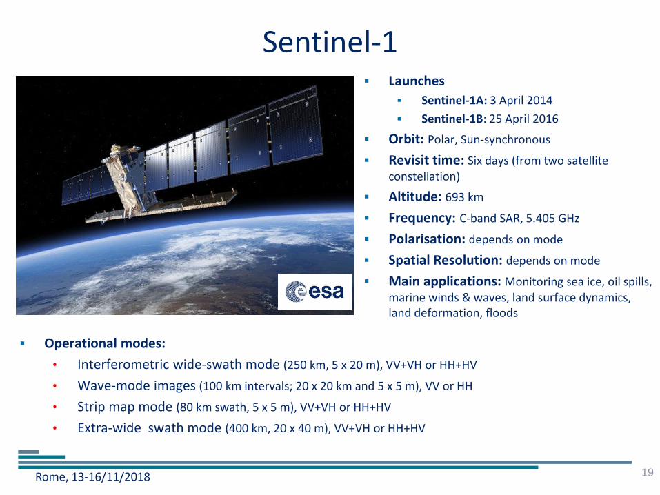
Sentinel-1
19
Launches
Sentinel-1A: 3 April 2014
Sentinel-1B: 25 April 2016
Orbit: Polar, Sun-synchronous
Revisit time: Six days (from two satellite constellation)
Altitude: 693 km
Frequency: C-band SAR, 5.405 GHz
Polarisation: depends on mode
Spatial Resolution: depends on mode
Main applications: Monitoring sea ice, oil spills, marine winds & waves, land surface dynamics, land deformation, floods
Operational modes:
• Interferometric wide-swath mode (250 km, 5 x 20 m), VV+VH or HH+HV
• Wave-mode images (100 km intervals; 20 x 20 km and 5 x 5 m), VV or HH
• Strip map mode (80 km swath, 5 x 5 m), VV+VH or HH+HV
• Extra-wide swath mode (400 km, 20 x 40 m), VV+VH or HH+HV
Rome, 13-16/11/2018
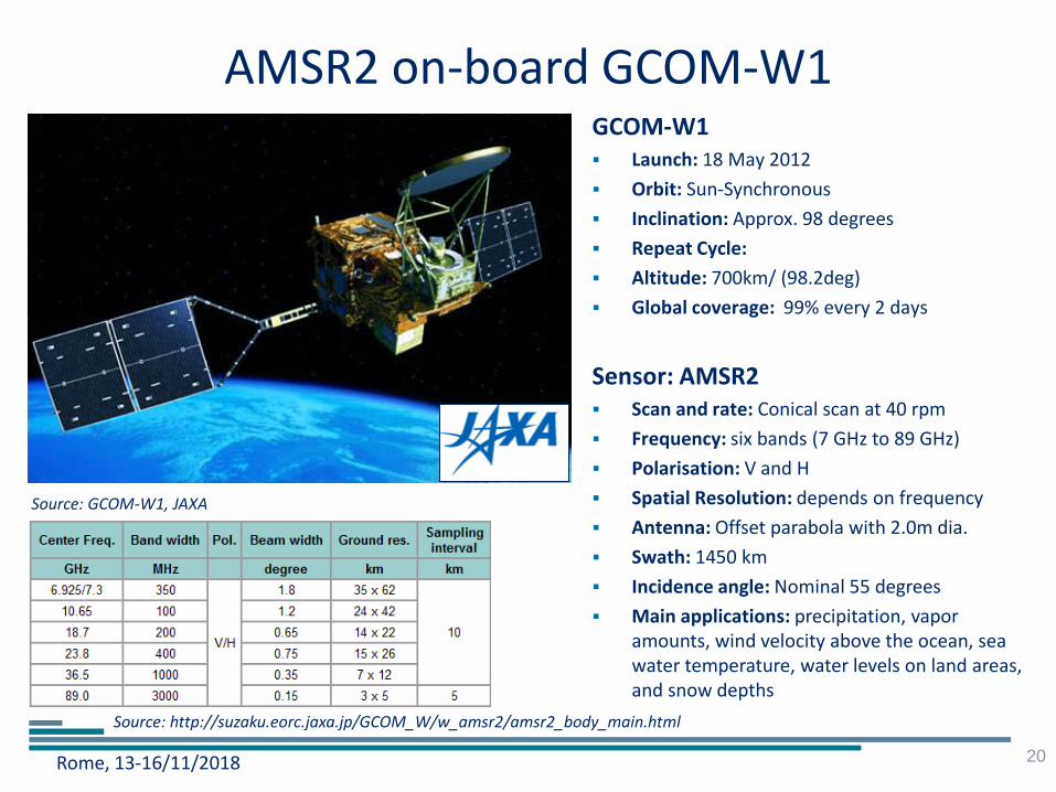
AMSR2 on-board GCOM-W1
20
GCOM-W1 Launch: 18 May 2012
Orbit: Sun-Synchronous
Inclination: Approx. 98 degrees
Repeat Cycle:
Altitude: 700km/ (98.2deg)
Global coverage: 99% every 2 days
Source: GCOM-W1, JAXA
Source: http://suzaku.eorc.jaxa.jp/GCOM_W/w_amsr2/amsr2_body_main.html
Sensor: AMSR2 Scan and rate: Conical scan at 40 rpm
Frequency: six bands (7 GHz to 89 GHz)
Polarisation: V and H
Spatial Resolution: depends on frequency
Antenna: Offset parabola with 2.0m dia.
Swath: 1450 km
Incidence angle: Nominal 55 degrees
Main applications: precipitation, vapor amounts, wind velocity above the ocean, sea water temperature, water levels on land areas, and snow depths
Rome, 13-16/11/2018
The Expectation
21
“…, L-band [soil moisture] retrievals can be performed
and meet the science requirements. In contrast, C- and
X-band measurements are representative of the top 1 cm or
less of soil. Moderate vegetation (greater than ~3 kg m-2)
attenuates the signal sufficiently at these frequencies to make
the measurements relatively insensitive to soil moisture.”
Entekhabi, D., Njoku, E.G., O'Neill, P.E., Kellog, K.H., Crow, W.T., Edelstein, W.N., Entin, J.K., Goodman, S.D., Jackson, T.J., Johnson, J., Kimball, J., Piepmeier, J.R., Koster, R., Martin, N., McDonald, K.C., Moghaddam, M., Moran, S., Reichle, R., Shi, J.C., Spencer, M.W., Thurman, S.W., Tsang, L., & Van Zyl, J. (2010). The Soil Moisture Active Passive (SMAP) mission. Proceedings of the IEEE, 98, 704-716
Rome, 13-16/11/2018
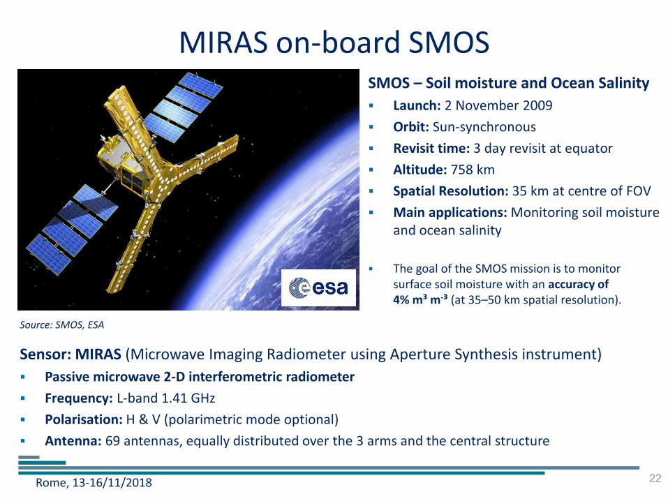
MIRAS on-board SMOS
22
SMOS – Soil moisture and Ocean Salinity
Launch: 2 November 2009
Orbit: Sun-synchronous
Revisit time: 3 day revisit at equator
Altitude: 758 km
Spatial Resolution: 35 km at centre of FOV
Main applications: Monitoring soil moisture and ocean salinity
The goal of the SMOS mission is to monitor surface soil moisture with an accuracy of 4% m³ m-³ (at 35–50 km spatial resolution).
Source: SMOS, ESA
Sensor: MIRAS (Microwave Imaging Radiometer using Aperture Synthesis instrument)
Passive microwave 2-D interferometric radiometer
Frequency: L-band 1.41 GHz
Polarisation: H & V (polarimetric mode optional)
Antenna: 69 antennas, equally distributed over the 3 arms and the central structure

Rome, 13-16/11/2018
SMAP – Soil Moisture Active Passive • Launch: 31 January 2015
• Orbit: near-polar, sun-synchronous orbit
• Revisit time: global coverage within 3 days at the equator and 2 days at boreal latitudes (> 45 degrees N)
• Altitude: 680 km
• Polarisation: depends on instrument
• Spatial Resolution:
– Radiometer: (IFOV): 39 km x 47 km
– Radar: 1-3 km (over outer 70% of swath)
• Rotation rate: 14.6 RPM
• Main applications: weather & climate forecasting, drought, floods & landslides
23
Source: SMAP, NASA, https://smap.jpl.nasa.gov/instrument/ Radiometer
• Frequency: 1.41 GHz
• Polarizations: H, V, 3rd & 4th Stokes
• Relative accuracy (30 km grid): 1.3 K
• Data collection:
– High-rate (sub-band) data acquired over land
– Low-rate data acquired globally
Radar (failure in July 2015)
• Frequency: 1.26 GHz
• Polarizations: VV, HH, HV (not fully polarimetric)
• Relative accuracy (3 km grid): 1 dB (HH and VV), 1.5 dB (HV)
• Data collection:
– High-resolution (SAR) data acquired over land
– Low-resolution data acquired globally
Rome, 13-16/11/2018
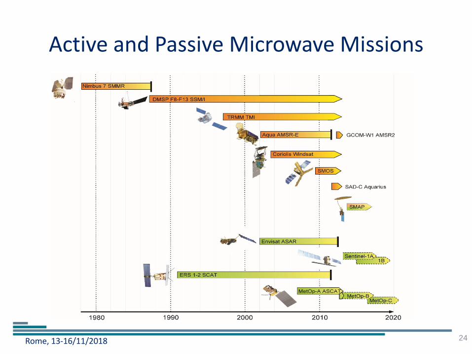
Active and Passive Microwave Missions
24

Rome, 13-16/11/2018
Sampling Requirements
25
Rome, 13-16/11/2018
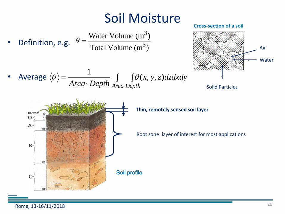
Soil Moisture
• Definition, e.g.
• Average
Area Depth
dzdxdyzyxDepthArea
),,(1
26
Thin, remotely sensed soil layer
Root zone: layer of interest for most applications
Soil profile
)(m Volume Total
)(m VolumeWater 3
3
Air
Water
Solid Particles
Cross-section of a soil
Rome, 13-16/11/2018
Scaling Issues
27
• The term “scale” refers to a – characteristic length – characteristic time
• The concept of scale can be applied to – Process scale = typical time and length scales at which a process takes
place – Measurement scale = spatial and temporal sampling characteristics of the
sensor system – Model scale = Mathematical/physical description of a process
Ideally: Process = Measurement = Model scale
• Microwave remote sensing offers a large suit of sensors
– Scaling issues must be understood in order to select the most suitable sensors for the application
Rome, 13-16/11/2018
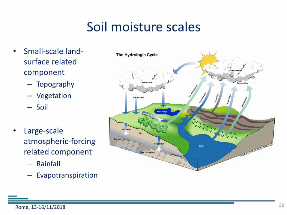
Soil moisture scales
• Small-scale land-surface related component
– Topography
– Vegetation
– Soil
• Large-scale atmospheric-forcing related component
– Rainfall
– Evapotranspiration
28
Rome, 13-16/11/2018
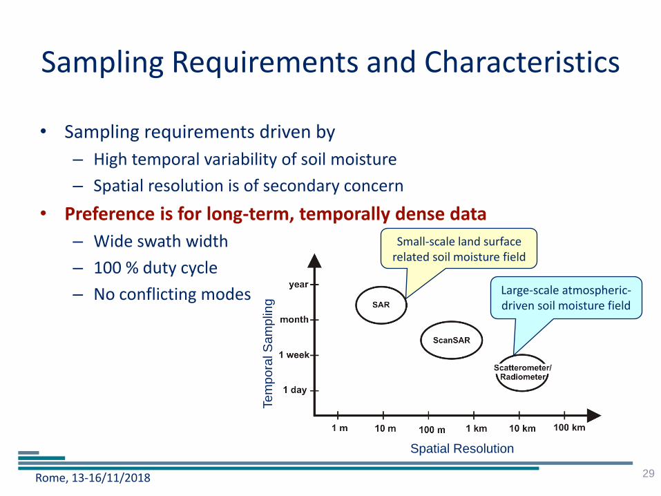
Sampling Requirements and Characteristics
• Sampling requirements driven by
– High temporal variability of soil moisture
– Spatial resolution is of secondary concern
• Preference is for long-term, temporally dense data
– Wide swath width
– 100 % duty cycle
– No conflicting modes
29
Small-scale land surface related soil moisture field
Large-scale atmospheric-driven soil moisture field
Te
mp
ora
l S
am
plin
g
Spatial Resolution
Rome, 13-16/11/2018
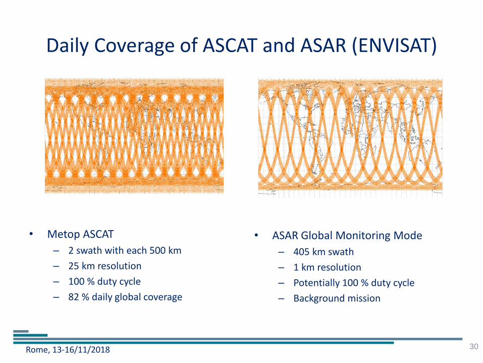
Daily Coverage of ASCAT and ASAR (ENVISAT)
• Metop ASCAT
– 2 swath with each 500 km
– 25 km resolution
– 100 % duty cycle
– 82 % daily global coverage
30
• ASAR Global Monitoring Mode
– 405 km swath
– 1 km resolution
– Potentially 100 % duty cycle
– Background mission
Rome, 13-16/11/2018
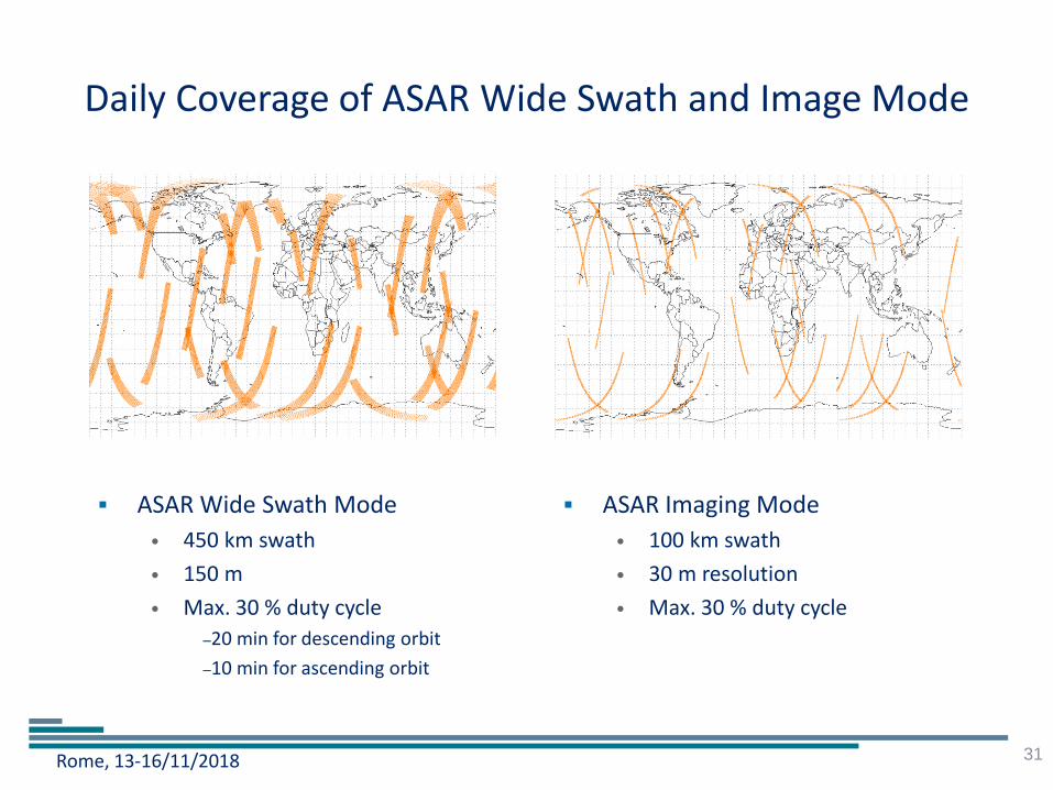
Daily Coverage of ASAR Wide Swath and Image Mode
31
ASAR Wide Swath Mode
• 450 km swath
• 150 m
• Max. 30 % duty cycle
–20 min for descending orbit
–10 min for ascending orbit
ASAR Imaging Mode
• 100 km swath
• 30 m resolution
• Max. 30 % duty cycle

Rome, 13-16/11/2018
Spatio-Temporal Sampling of ASCAT Daily global ASCAT coverage achieved by METOP-A and METOP-B constellation
Wagner et al. (2013) The ASCAT soil moisture product: A review of its specifications,
validation results, and emerging applications, Meteorologische Zeitschrift, 22(1), 5-33.
Rome, 13-16/11/2018
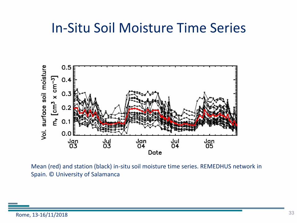
In-Situ Soil Moisture Time Series
33
Mean (red) and station (black) in-situ soil moisture time series. REMEDHUS network in Spain. © University of Salamanca
Rome, 13-16/11/2018
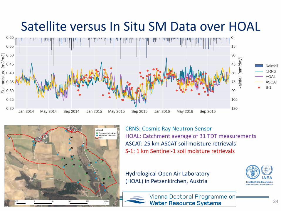
Satellite versus In Situ SM Data over HOAL
34
CRNS: Cosmic Ray Neutron Sensor HOAL: Catchment average of 31 TDT measurements ASCAT: 25 km ASCAT soil moisture retrievals S-1: 1 km Sentinel-1 soil moisture retrievals Hydrological Open Air Laboratory (HOAL) in Petzenkirchen, Austria
Rome, 13-16/11/2018
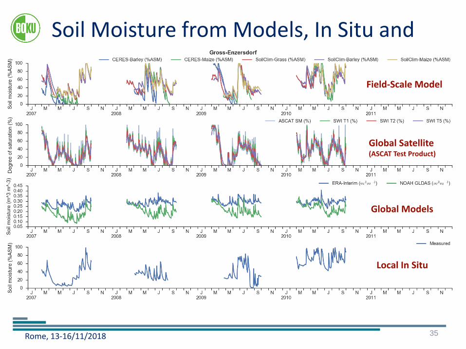
Soil Moisture from Models, In Situ and Satellites
35
Field-Scale Model
Global Satellite (ASCAT Test Product)
Global Models
Local In Situ
Rome, 13-16/11/2018
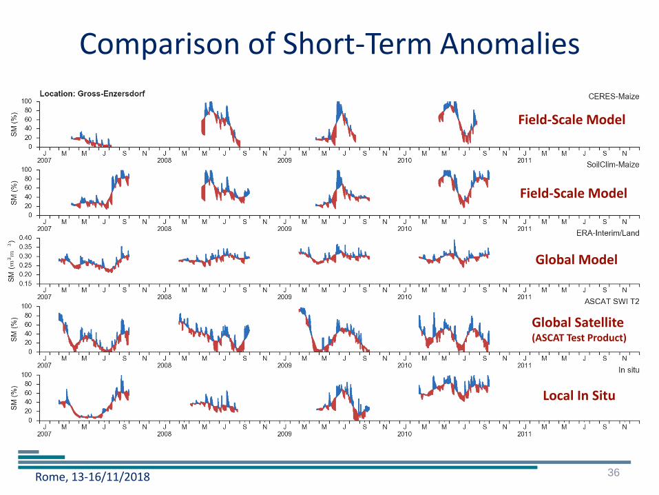
Comparison of Short-Term Anomalies
36
Field-Scale Model
Global Satellite (ASCAT Test Product)
Field-Scale Model
Global Model
Local In Situ
Rome, 13-16/11/2018
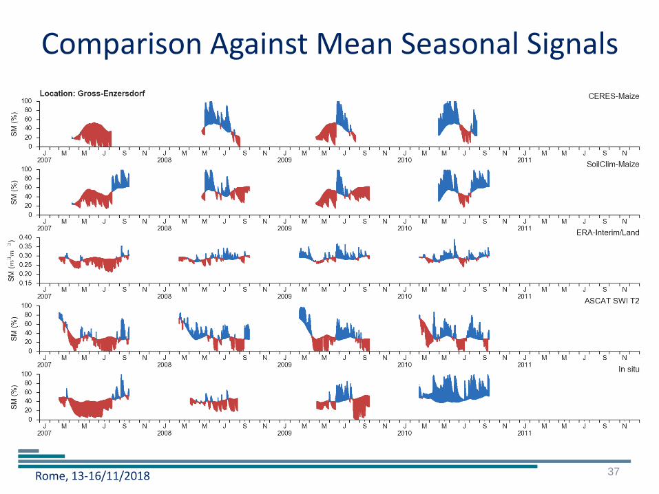
Comparison Against Mean Seasonal Signals
37
Rome, 13-16/11/2018
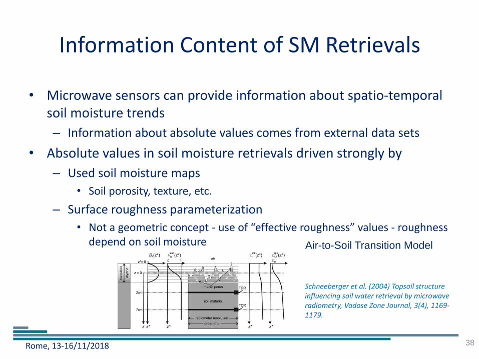
Information Content of SM Retrievals
• Microwave sensors can provide information about spatio-temporal soil moisture trends
– Information about absolute values comes from external data sets
• Absolute values in soil moisture retrievals driven strongly by
– Used soil moisture maps
• Soil porosity, texture, etc.
– Surface roughness parameterization
• Not a geometric concept - use of “effective roughness” values - roughness depend on soil moisture
38
Schneeberger et al. (2004) Topsoil structure influencing soil water retrieval by microwave radiometry, Vadose Zone Journal, 3(4), 1169-1179.
Air-to-Soil Transition Model

Rome, 13-16/11/2018
Retrieval Approaches
39
Rome, 13-16/11/2018
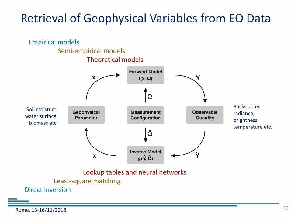
Retrieval of Geophysical Variables from EO Data
40
Empirical models Semi-empirical models Theoretical models
Lookup tables and neural networks Least-square matching Direct inversion
Soil moisture, water surface,
biomass etc.
Backscatter, radiance, brightness temperature etc.
Rome, 13-16/11/2018
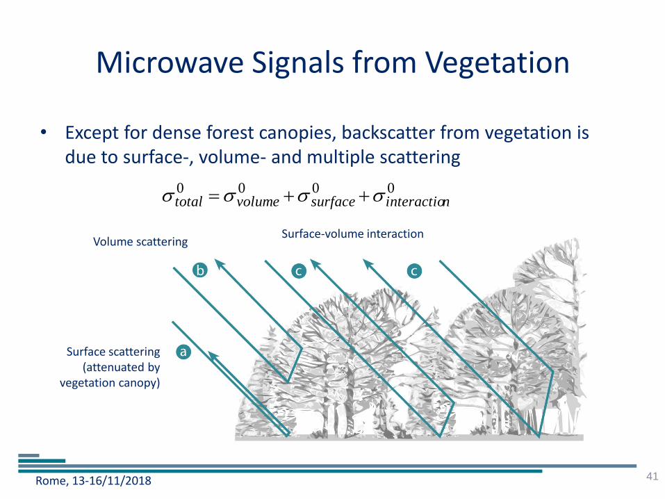
Microwave Signals from Vegetation
• Except for dense forest canopies, backscatter from vegetation is due to surface-, volume- and multiple scattering
41
Surface scattering (attenuated by
vegetation canopy)
Volume scattering Surface-volume interaction
0000ninteractiosurfacevolumetotal
Rome, 13-16/11/2018
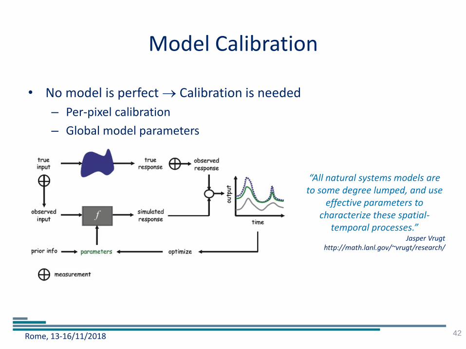
Model Calibration
• No model is perfect Calibration is needed
– Per-pixel calibration
– Global model parameters
42
“All natural systems models are to some degree lumped, and use
effective parameters to characterize these spatial-
temporal processes.” Jasper Vrugt
http://math.lanl.gov/~vrugt/research/
Rome, 13-16/11/2018
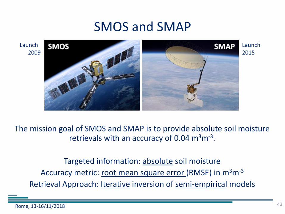
SMOS and SMAP
The mission goal of SMOS and SMAP is to provide absolute soil moisture retrievals with an accuracy of 0.04 m3m-3.
Targeted information: absolute soil moisture
Accuracy metric: root mean square error (RMSE) in m3m-3
Retrieval Approach: Iterative inversion of semi-empirical models
43
Launch 2009
Launch 2015
Rome, 13-16/11/2018
Working Hypothesis for ASCAT Soil Moisture Retrieval
• Information about absolute soil moisture content comes from soil maps, not the satellite
• ASCAT data are not fundamentally different to SMOS or SMAP. Nonetheless, for ASCAT we have always stressed that the information content lies in the relative variation of the observations
– This has resulted in a disparate treatment of ASCAT and SMOS data in the literature
• ASCAT data have often been referred to as soil moisture index
• ASCAT users approached the problem with less expectations
• ASCAT soil moisture data are represented in degree of saturation
– Unit 0-1 or 0-100 %
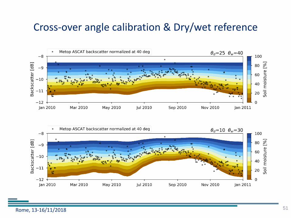
– Dry and wet reference values are extracted from multi-year time series
– Conversion to absolute values possible if soil porosity and soil moisture residual content are known
44

Rome, 13-16/11/2018
TU Wien Backscatter Model
• Motivated by physical models and empirical evidence
– Formulated in decibels (dB) domain
– Linear relationship between backscatter (in dB) and soil moisture
– Empirical description of incidence angle behaviour
– Seasonal vegetation effects cancel each other out at the "cross-over angles"
• dependent on soil moisture
45
ERS Scatterometer measurements
Incidence angle behaviour is determined by vegetation and roughness roughness
Changes due to soil moisture variations
Rome, 13-16/11/2018
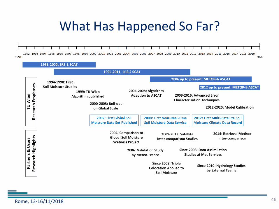
What Has Happened So Far?
46
Rome, 13-16/11/2018
TU Wien Model: Remarkably Stable Since 1998
• In its core algorithms, the TU Wien model is still the same as in 1998 • Algorithmic improvements have dealt with
– Calibration/model parameter estimation – Azimuthal effects – Temporal behaviour of 𝜎0 𝜃 – Error propagation
• Algorithmic progress has been slower than wished-for due to – Rapidly growing user community
• Already thousands of direct and indirect users
– Constraints imposed by operational nature of data service – Need to improve software (IDL Python)
• Performance, tractability, quality control, modularisation, versioning, …
– Lack of high-quality reference data – Lack of in-biased validation techniques – Major shortcomings of available theoretical models
47
Rome, 13-16/11/2018
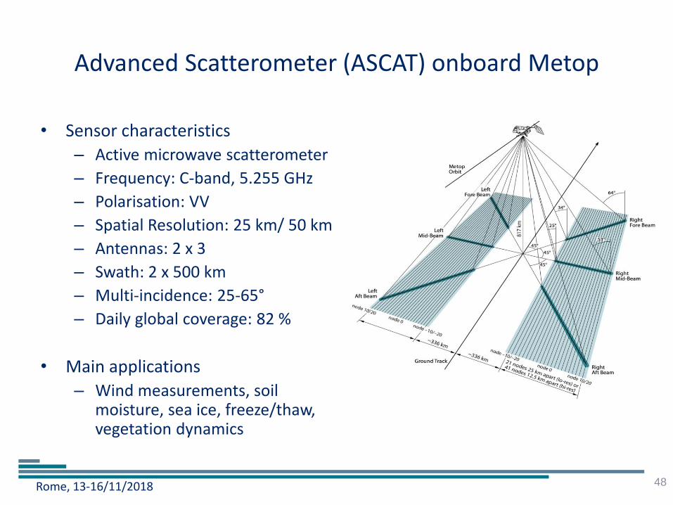
Advanced Scatterometer (ASCAT) onboard Metop
• Sensor characteristics
– Active microwave scatterometer
– Frequency: C-band, 5.255 GHz
– Polarisation: VV
– Spatial Resolution: 25 km/ 50 km
– Antennas: 2 x 3
– Swath: 2 x 500 km
– Multi-incidence: 25-65°
– Daily global coverage: 82 %
• Main applications
– Wind measurements, soil moisture, sea ice, freeze/thaw, vegetation dynamics
48
Rome, 13-16/11/2018
TU Wien Change Detection Approach
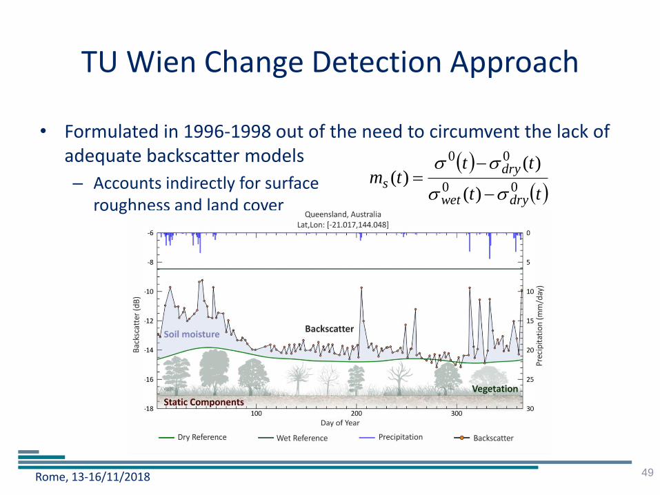
• Formulated in 1996-1998 out of the need to circumvent the lack of adequate backscatter models
– Accounts indirectly for surface roughness and land cover
49
tt
tttm
drywet
drys 00
00
)(
)()(
Rome, 13-16/11/2018
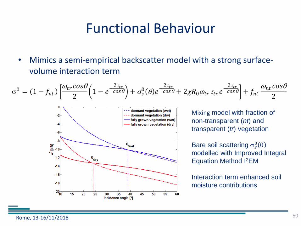
Functional Behaviour
• Mimics a semi-empirical backscatter model with a strong surface-volume interaction term
50
Mixing model with fraction of
non-transparent (nt) and
transparent (tr) vegetation
Bare soil scattering 𝑠0
modelled with Improved Integral
Equation Method I2EM
Interaction term enhanced soil
moisture contributions
0 = 1 − 𝑓𝑛𝑡 𝑡𝑟𝑐𝑜𝑠
2 1 − 𝑒
−2𝑡𝑟𝑐𝑜𝑠 + 𝑠
0 𝑒−
2𝑡𝑟𝑐𝑜𝑠 + 2𝑅0𝑡𝑟 𝑡𝑟𝑒
−2𝑡𝑟𝑐𝑜𝑠 + 𝑓𝑛𝑡
𝑛𝑡 𝑐𝑜𝑠
2
Rome, 13-16/11/2018
Cross-over angle calibration & Dry/wet reference
51
Rome, 13-16/11/2018
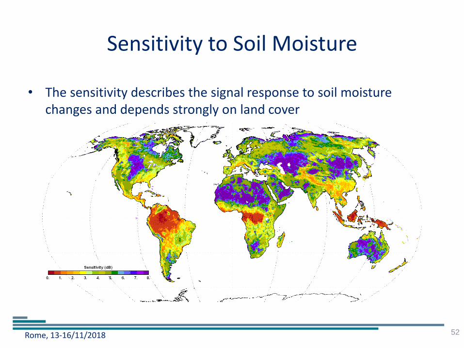
Sensitivity to Soil Moisture
• The sensitivity describes the signal response to soil moisture changes and depends strongly on land cover
52

Rome, 13-16/11/2018
Metop ASCAT Surface Soil Moisture Climatology
53
Rome, 13-16/11/2018
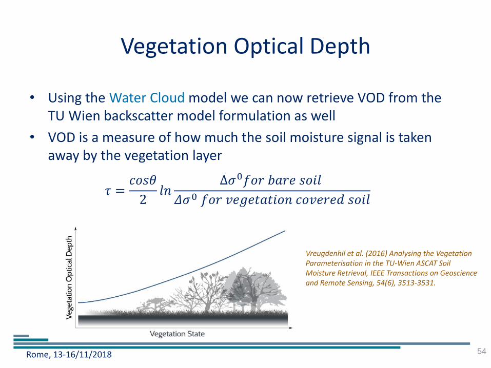
Vegetation Optical Depth
• Using the Water Cloud model we can now retrieve VOD from the TU Wien backscatter model formulation as well
• VOD is a measure of how much the soil moisture signal is taken away by the vegetation layer
54
𝜏 =𝑐𝑜𝑠𝜃
2𝑙𝑛
Δ𝜎0𝑓𝑜𝑟 𝑏𝑎𝑟𝑒 𝑠𝑜𝑖𝑙
𝛥𝜎0 𝑓𝑜𝑟 𝑣𝑒𝑔𝑒𝑡𝑎𝑡𝑖𝑜𝑛 𝑐𝑜𝑣𝑒𝑟𝑒𝑑 𝑠𝑜𝑖𝑙
Vreugdenhil et al. (2016) Analysing the Vegetation Parameterisation in the TU-Wien ASCAT Soil Moisture Retrieval, IEEE Transactions on Geoscience and Remote Sensing, 54(6), 3513-3531.
Rome, 13-16/11/2018
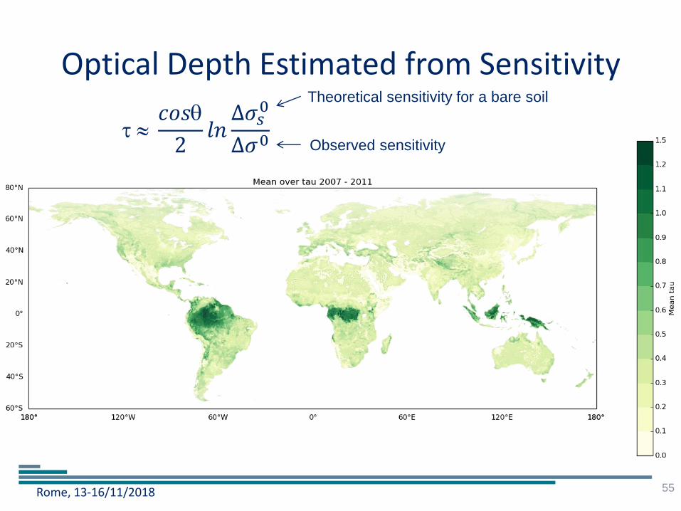
Optical Depth Estimated from Sensitivity
55
𝑐𝑜𝑠
2𝑙𝑛
∆𝜎𝑠0
Δ𝜎0
Theoretical sensitivity for a bare soil
Observed sensitivity
Rome, 13-16/11/2018
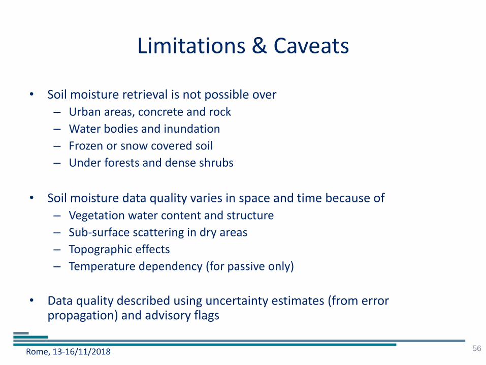
Limitations & Caveats
• Soil moisture retrieval is not possible over
– Urban areas, concrete and rock
– Water bodies and inundation
– Frozen or snow covered soil
– Under forests and dense shrubs
• Soil moisture data quality varies in space and time because of
– Vegetation water content and structure
– Sub-surface scattering in dry areas
– Topographic effects
– Temperature dependency (for passive only)
• Data quality described using uncertainty estimates (from error propagation) and advisory flags
56

Rome, 13-16/11/2018
Sentinel-1 – A Game Changer • C-band SAR satellite in
continuation of ERS-1/2 and ENVISAT
• High spatio-temporal coverage
– Spatial resolution 20-80 m
– Temporal resolution < 3 days over Europe and Canada
• with 2 satellites
• Excellent data quality
• Highly dynamic land surface processes can be captured
– Impact on water management, health and other applications could be high if the challenges in the ground segment can be overcome
Solar panel and SAR antenna of Sentinel-1
launched 3 April 2014. Image was acquired by
the satellite's onboard camera. © ESA
Rome, 13-16/11/2018
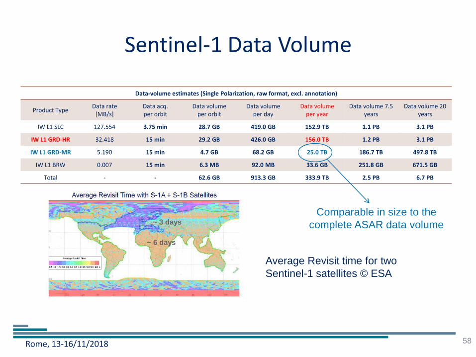
Sentinel-1 Data Volume
58
Data-volume estimates (Single Polarization, raw format, excl. annotation)
Product Type Data rate
[MB/s] Data acq. per orbit
Data volume per orbit
Data volume per day
Data volume per year
Data volume 7.5 years
Data volume 20 years
IW L1 SLC 127.554 3.75 min 28.7 GB 419.0 GB 152.9 TB 1.1 PB 3.1 PB
IW L1 GRD-HR 32.418 15 min 29.2 GB 426.0 GB 156.0 TB 1.2 PB 3.1 PB
IW L1 GRD-MR 5.190 15 min 4.7 GB 68.2 GB 25.0 TB 186.7 TB 497.8 TB
IW L1 BRW 0.007 15 min 6.3 MB 92.0 MB 33.6 GB 251.8 GB 671.5 GB
Total - - 62.6 GB 913.3 GB 333.9 TB 2.5 PB 6.7 PB
Average Revisit time for two
Sentinel-1 satellites © ESA
~ 6 days
~ 3 days
Comparable in size to the
complete ASAR data volume
Rome, 13-16/11/2018
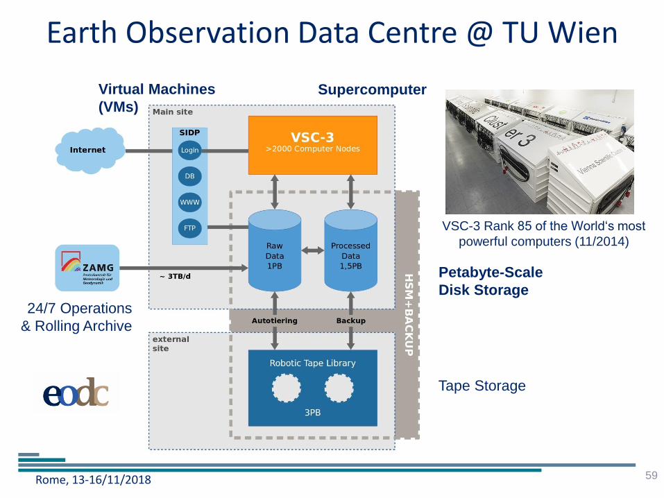
Earth Observation Data Centre @ TU Wien
59
24/7 Operations
& Rolling Archive
Petabyte-Scale
Disk Storage
Supercomputer
Tape Storage
Virtual Machines
(VMs)
VSC-3 Rank 85 of the World‘s most
powerful computers (11/2014)
Rome, 13-16/11/2018
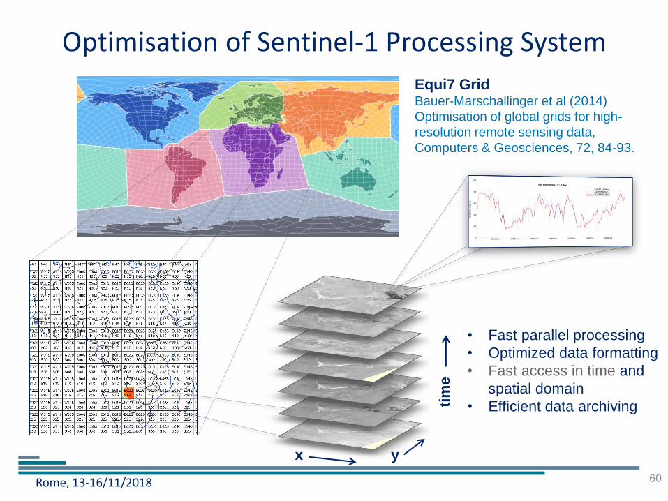
x y ti
me
Optimisation of Sentinel-1 Processing System
60
• Fast parallel processing
• Optimized data formatting
• Fast access in time and
spatial domain
• Efficient data archiving
Equi7 Grid Bauer-Marschallinger et al (2014)
Optimisation of global grids for high-
resolution remote sensing data,
Computers & Geosciences, 72, 84-93.

Rome, 13-16/11/2018
Summary
61
Rome, 13-16/11/2018
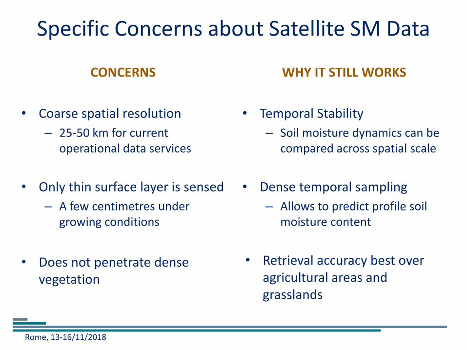
CONCERNS
• Coarse spatial resolution
– 25-50 km for current operational data services
• Only thin surface layer is sensed
– A few centimetres under growing conditions
• Does not penetrate dense vegetation
WHY IT STILL WORKS
• Temporal Stability
– Soil moisture dynamics can be compared across spatial scale
• Dense temporal sampling
– Allows to predict profile soil moisture content
• Retrieval accuracy best over agricultural areas and grasslands
Specific Concerns about Satellite SM Data
Rome, 13-16/11/2018
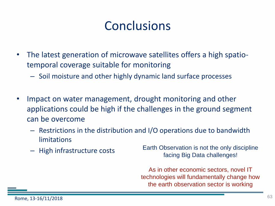
Conclusions
• The latest generation of microwave satellites offers a high spatio-temporal coverage suitable for monitoring
– Soil moisture and other highly dynamic land surface processes
• Impact on water management, drought monitoring and other applications could be high if the challenges in the ground segment can be overcome
– Restrictions in the distribution and I/O operations due to bandwidth limitations
– High infrastructure costs
63
Earth Observation is not the only discipline
facing Big Data challenges!
As in other economic sectors, novel IT
technologies will fundamentally change how
the earth observation sector is working
Rome, 13-16/11/2018
References - Books
• Jensen, J.R. (2006): Remote Sensing of the Environment: An Earth Resource Perspective (2nd Edition). Pearson, ISBN:978-0131889508
• Tipler, P.A. (2000): Physik. Spektrum Akademischer Verlag, ISBN: 978-3860251225
• F. T. Ulaby, R. K. Moore, and A. K. Fung, Microwave Remote Sensing: Active and Passive. Vol. III - Volume Scattering and Emission Theory, Advanced Systems and Applications. Artech House, Inc.
64

Rome, 13-16/11/2018
References - Technical Report
• ASCAT Product Guide, Tech. Rep. Doc. No: EUM/OPS-EPS/MAN/04/0028, v5, 2015.
• Algorithm Theoretical Baseline Document (ATBD) Soil Moisture Data Records, Metop ASCAT Soil Moisture Time Series, Tech. Rep. Doc. No: SAF/HSAF/CDOP3/ATBD, v0.7, 2018.
• Algorithm Theoretical Baseline Document (ATBD) Soil Moisture NRT, Metop ASCAT Soil Moisture Orbit, Tech. Rep. Doc. No: SAF/HSAF/CDOP2/ATBD, v0.4, 2016.
65
Rome, 13-16/11/2018
References - Articles
• Z. Bartalis, K. Scipal, and W. Wagner, Azimuthal anisotropy of scatterometer measurements over land, vol. 44, no. 8, pp. 2083–2092.
• Z. Bartalis, W. Wagner, V. Naeimi, S. Hasenauer, K. Scipal, H. Bonekamp, J. Figa, and C. Anderson, Initial soil moisture retrievals from the METOP-a advanced scatterometer (ASCAT), vol. 34.
• J. Figa-Saldana, J. J. W. Wilson, E. Attema, R. Gelsthorpe, M. R. Drinkwater, and A. Stoffelen, The Advanced Scatterometer (ASCAT) on the Meteorological Operational (MetOp) Platform: A follow on for European Wind Scatterometers, Canadian Journal of Remote Sensing, vol. 28, no. 3, pp. 404–412, 2002.
• R. V. Gelsthorpe, E. Schied, and J. J. W. Wilson, ASCAT - MetOp’s Advanced Scatterometer, ESA Bull. ISSN 0376-4265, vol. 102, pp. 19–27, 2000.
• V. Naeimi, K. Scipal, Z. Bartalis, S. Hasenauer, and W. Wagner, An improved soil moisture retrieval algorithm for ERS and METOP scatterometer observations, vol. 47, no. 7, pp. 1999–2013.
• W. Wagner, G. Lemoine, and H. Rott, A method for estimating soil moisture from ERS scatterometer and soil data, vol. 70, no. 2, pp. 191–207.
• W. Wagner, J. Noll, M. Borgeaud, and H. Rott, Monitoring soil moisture over the Canadian prairies with the ERS scatterometer, vol. 37, pp. 206–216.
• W. Wagner, G. Lemoine, M. Borgeaud, and H. Rott, A study of vegetation cover effects on ERS scatterometer data, vol. 37, no. 2II, pp. 938–948.
66


