
Air Force Institute of TechnologyAFIT Scholar
Theses and Dissertations Student Graduate Works
3-23-2017
Refugees in Urban Environments: Social,Economic, and Infrastructure ImpactsGarrett L. Jameson
Follow this and additional works at: https://scholar.afit.edu/etd
Part of the Operations Research, Systems Engineering and Industrial Engineering Commons,and the Public Affairs, Public Policy and Public Administration Commons
This Thesis is brought to you for free and open access by the Student Graduate Works at AFIT Scholar. It has been accepted for inclusion in Theses andDissertations by an authorized administrator of AFIT Scholar. For more information, please contact [email protected].
Recommended CitationJameson, Garrett L., "Refugees in Urban Environments: Social, Economic, and Infrastructure Impacts" (2017). Theses andDissertations. 1643.https://scholar.afit.edu/etd/1643

REFUGEES IN URBAN ENVIRONMENTS: SOCIAL, ECONOMIC, AND INFRASTRUCTURE IMPACTS
THESIS
Garrett L. Jameson, Second Lieutenant, USAF
AFIT-ENS-MS-17-M-136
DEPARTMENT OF THE AIR FORCE AIR UNIVERSITY
AIR FORCE INSTITUTE OF TECHNOLOGY
Wright-Patterson Air Force Base, Ohio
DISTRIBUTION STATEMENT A. APPROVED FOR PUBLIC RELEASE; DISTRIBUTION UNLIMITED.

The views expressed in this thesis are those of the author and do not reflect the official policy or position of the United States Air Force, the Department of Defense, or the United States Government. This material is declared a work of the U.S. Government and is not subject to copyright protection in the United States.

AFIT-ENS-MS-17-M-136
REFUGEES IN URBAN ENVIRONMENTS: SOCIAL, ECONOMIC, AND INFRASTRUCTURE IMPACTS
THESIS
Presented to the Faculty
Department of Operational Sciences
Graduate School of Engineering and Management
Air Force Institute of Technology
Air University
Air Education and Training Command
In Partial Fulfillment of the Requirements for the
Degree of Master of Science in Operations Research
Garrett L. Jameson, BS
Second Lieutenant, USAF
March 2017
DISTRIBUTION STATEMENT A. APPROVED FOR PUBLIC RELEASE; DISTRIBUTION UNLIMITED.

AFIT-ENS-MS-17-M-136
REFUGEES IN URBAN ENVIRONMENTS: SOCIAL, ECONOMIC, AND INFRASTRUCTURE IMPACTS
Garrett L. Jameson, BS
Second Lieutenant, USAF
Committee Membership:
Dr. Richard F. Deckro Chair
Lt Col Matthew J. Robbins, Ph.D. Member
iv
AFIT-ENS-MS-17-M-136
Abstract
The United Nations High Commissioner for Refugees has estimated that in 2015 there
were 21.3 million refugees worldwide; it is estimated that 1.8 million of these persons
were newly displaced during 2015. As refugees leave their country to seek the protection
of another nation’s government, they generally flow into urban areas. The impact of this
flow on cities and on the refugees, themselves, is not fully understood. This study is
focused on the impact of government policy decisions on the social, legal, and economic
integration of refugees within an urban environment. Investigation into this topic resulted
in the development of a system dynamics model representing the city of Rotterdam, the
Netherlands. The results of a designed experiment on the model indicate that economic
policy directed towards refugees or specific ethnic groups results in positive trends of
integration within a city system. This pilot study provides insight into the impacts of
refugee flow and policy decisions within the applied context of an urban model.

v
Acknowledgments
I would like to thank my faculty advisor, Dr. Richard Deckro, for his guidance and
support throughout the course of this thesis effort. Your assistance in the exploration of
this topic is much appreciated. Our discussions over the past year have been enlightening
and enjoyable. I would like to thank my reader, Lt Col Matthew Robinson, for his inputs
as an editor of this thesis document. His suggestions have significantly improved the
quality of this thesis, as well as my skill as a writer. Both of these individuals have made
substantial, positive contributions to my learning experience. Thank you.
Garrett Jameson

vi
Table of Contents
Page
Abstract .............................................................................................................................. iv
Table of Contents ............................................................................................................... vi
List of Figures .................................................................................................................. viii
I. Introduction .....................................................................................................................1
II. Literature Review ............................................................................................................8
Overview ......................................................................................................................8
Refugee Definition .......................................................................................................8
Refugee Situation .........................................................................................................9
Refugee Studies ..........................................................................................................11
Refugee Integration ....................................................................................................15
Ethnic Enclaves ..........................................................................................................18
City Definition ............................................................................................................20
Urbanization ...............................................................................................................21
City Models ................................................................................................................24
Summary.....................................................................................................................36
III. The Netherlands ...........................................................................................................37
Overview ....................................................................................................................37
Selection of the Netherlands for Model......................................................................37
Brief History of Dutch Integration Policy ..................................................................38
Current Integration Program .......................................................................................41
Refugee Studies, Netherlands .....................................................................................44
Summary.....................................................................................................................47

vii
IV. Model Development ....................................................................................................48
Overview ....................................................................................................................48
Model Purpose ............................................................................................................48
Model Subsystems ......................................................................................................50
Model Validation ........................................................................................................89
Summary...................................................................................................................105
V. Analysis and Results ...................................................................................................107
Overview ..................................................................................................................107
Results and Discussion .............................................................................................107
Summary...................................................................................................................115
VI. Conclusions and Recommendations ..........................................................................116
Overview ..................................................................................................................116
Conclusions of Research ..........................................................................................116
Limitations of Results...............................................................................................117
Recommendations for Future Research....................................................................118
Significance of Research ..........................................................................................120
Summary...................................................................................................................121
Appendix A: Supplemental Tables ..................................................................................122
Appendix B: Vensim Model Code ...................................................................................125
Appendix C: Storyboard ..................................................................................................172
Bibliography ....................................................................................................................173

viii
List of Figures
Page
Figure 1: Cellular automata rule set .................................................................................. 25
Figure 2: Cellular automata model at time steps 0, 1, and 5 ............................................. 25
Figure 3: Simple feedback loop. Adapted from Forrester [45]. ........................................ 30
Figure 4: Land Use Subsystem ......................................................................................... 53
Figure 5: MHLM MI housing land multiplier i[i] lookup curve ...................................... 54
Figure 6: Job Market Subsystem....................................................................................... 62
Figure 7: Population Total '07-'14 .................................................................................... 70
Figure 8: People Subsystem .............................................................................................. 73
Figure 9: Legal Subsystem................................................................................................ 76
Figure 10: Primary education and transitional secondary education ................................ 79
Figure 11: Secondary education ........................................................................................ 80
Figure 12: Education subsystem ....................................................................................... 82
Figure 13: Cognitive dissonance lookup curve ................................................................. 88
Figure 14: Language multiplier s-curve ............................................................................ 89
Figure 15: UDRI model system’s mapping ...................................................................... 90
Figure 16: Sectors of income; autochtonen vs. non-refugee, non-western allochtonen ... 93
Figure 17: Sectors of income; autochtonen vs. non-refugee western allochtonen ........... 94
Figure 18: Sectors of income; autochtonen vs. non-western allochtonen refugee ........... 95
Figure 19: Sectors of income; autochtonen vs. western allochtonen refugee ................... 95
Figure 20: Ratio of group by district, Centrum................................................................. 96

ix
Figure 21: Sensitivity of ratio LI of group working population: autochtonen, non-western
allochtonen, western allochtonen ............................................................................. 102
Figure 22: Sensitivity ratio group by district, Centrum: autochtonen, non-western
allochtonen, western allochtonen ............................................................................. 103
Figure 23: Experiment 1 social integration sensitivity graph, non-western allochtonen
refugees .................................................................................................................... 108
Figure 24: Experiment 1 legal integration sensitivity graph, non-western allochtonen
refugees .................................................................................................................... 110
Figure 25: Experiment 1 low income economic integration sensitivity graph, non-western
allochtonen refugees ................................................................................................. 111
Figure 26: Experiment 1 middle income economic integration sensitivity graph, non-
western allochtonen refugees ................................................................................... 111
Figure 27: Experiment 2 social integration sensitivity graph, non-western allochtonen
refugees .................................................................................................................... 112
Figure 28: Experiment 2 legal integration sensitivity graph, non-western allochtonen
refugees .................................................................................................................... 113
Figure 29: Experiment 2 low income economic integration sensitivity graph, non-western
allochtonen refugees ................................................................................................. 114
Figure 30: Experiment 2 middle income economic integration sensitivity graph, non-
western allochtonen refugees ................................................................................... 115

x
List of Tables
Page
Table 1: District to Index Mapping ................................................................................... 52
Table 2: SBI 2008 Classifications by Activities ............................................................... 61
Table 3: Initial proportion of sectors of income by group ................................................ 67
Table 4: Jobs per class by sector of income ...................................................................... 68
Table 5: Population and birth ratio by ethnic group ......................................................... 74
Table 6: Integration measures ........................................................................................... 85
Table 7: Social subsystem variable uses and justification ................................................ 87
Table 8: District geographic coordinates ........................................................................ 122
Table 9: Sensitivity analysis constants and values ......................................................... 122
Table 10: Experiment factors .......................................................................................... 123
Table 11: Experiment responses ..................................................................................... 124

1
I. Introduction
The United Nations High Commissioner for Refugees (UNHCR) [1] has
estimated the number of refugees worldwide in 2015 to be 21.3 million people. It is
estimated that 1.8 million of these persons were newly displaced in 2015 [1]. Refugees,
under the mandate of UNHCR, are those who migrate to other nations to seek protection
against persecution [2]. These persons are not the same as internally displaced persons
(estimated 40.8 million globally) or rural-urban migrants, who do not leave their country
yet travel to a different locale [1]. Rural-urban migrants are not tracked by UNHCR
because they are not considered to have been forcibly displaced. Generally, refugees are
uprooted from their home country due to violent conflict such as war.
It is estimated that 60% of refugees worldwide live in an urban environment; the
majority of these urban dwellers are living in private residences or refugee collective
centers [1]. The large number of urban refugees has led policy makers to question the
impact that refugees have on the city in which they reside. Is the job market resilient to a
flood of refugees? A source of new labor increases competition for jobs within the
employment system, potentially depressing wages. These new laborers can also fill
shortages in certain industries. Refugees who do not speak the language of the host
country will likely not be able to fully utilize their education and job-skills, leading to
underemployment and unemployment. The impact of refugee flow on economics is
related to the housing market within a city.
Is the housing market able to absorb the increase in population from refugees?
The trend of populations moving into urban areas is known as “urbanization.”
Urbanization has increased to the point where in 2007, for the first time in history, the
REFUGEES IN URBAN ENVIRONMENTS: SOCIAL, ECONOMIC,AND INFRASTRUCTURE IMPACTS

2
global urban population outnumbered the global rural population [3]. As urbanization
increases to an estimated 66% by 2050, the populations of cities are predicted to swell
[3]. The literature that addresses urbanization and migration are generally concerned with
internal, rural-urban migration processes and the economic impact of the migration [4]–
[6]. The research presented in this thesis attempts to bring more understanding to the
impact of refugee flow on city infrastructure.
Consequences of refugee migration should also be viewed from the perspective of
the refugees themselves. Refugees migrate to another nation under stressful
circumstances, with no job, an insecure living situation, and potentially no legal status.
They often face discrimination from some members of the host population [7]. There is a
large social toll that is taken on the refugees while living in the asylum of a host. Their
movement is often restricted and their rights limited while the host nation works to
integrate them [8]. Refugees are concerned about the same issues that city planners and
politicians are: jobs and housing [9]. How are refugees going to be able to provide for
and house their families? If the job market and housing markets are not able to absorb the
influx of refugees, then many will be left homeless and jobless. Refugees who do not
speak the language of their host nation and cannot find a secure living space or a job are
vulnerable. This vulnerability is worsened by discrimination from the host population;
refugees who do not feel integrated into their communities may feel victimized [10].
Even in an amiable community, refugees and other migrants may not desire to coalesce
into their new communities. The concepts of integration and economic and social
outcomes are explored further in the literature review chapter.

3
Much of the literature concerning refugees and migrant populations is found in
the fields of sociology and economics. An article by Phillimore and Goodson [11] aptly
describes the dual nature of refugee impact on the host nation and the refugees
themselves. Phillimore and Goodson [11] along with other authors [12]–[14] recommend
refugee policies and explore the impact of displacement on refugees. These studies are
well-founded in the literature but, at no fault of the authors, are qualitative in nature and
lack analytical rigor. Data availability is a significant problem in the attempt to analyze
refugees; many persons are not tracked accurately and certain concepts, such as
integration, are difficult to quantify. The economic studies concerning migrant
populations are largely focused on immigrant characteristics and their impact on
economic outcomes of the migrants themselves [15], [16]. These studies help to inform
the research presented in this thesis about the quantitative relationship between migrants
and economic outcomes; however, these and other studies are only a part of the
information needed to describe refugee integration and impact on cities.
The study of ethnic enclaves is a promising vein of research in quantifying
integration of migrants. Various studies that identify the causes of ethnic enclave
formation address the choices of the ethnic minority [17], [18]. Sociological and
economic research explains the impacts of living within an ethnic enclave on economic
and social integration [19], [20]. These and other studies help to inform the research
presented in this thesis about the interactions between refugee populations and the cities
into which they migrate.
The Department of Defense is especially concerned with the future of large cities.
Urban environments can be breeding grounds for terrorists, especially in areas where the

4
populace is, or perceives itself as, marginalized. Ethnic enclaves can socially and
economically isolate persons from the community at large, leading to a potential for
refugee victimhood (real or perceived) and facilitate recruitment by radicals [21]. Cities
by themselves affect global security; senior Department of Defense leaders identify cities
as economic and social centers (e.g., New York, Tokyo, and Lagos) that makes them
critical to both present and future global security [22]. Unemployment, competition for
resources, and feelings of victimization are drivers of instability within a city [23]. All are
likely outcomes of refugee flow into large cities with poor or insufficient infrastructure
and planning to deal with an increase in population. Sudden pressure can destabilize a
nation or a region. Various publications discuss cities as being centers for future conflict
[24], [25]. If cities are to be understood, then the impact of refugee flow into them must
be understood.
The Department of Defense has a vested interest in the impact of refugee flow
because of the potential impact on global security and the effects of Overseas
Contingency Operations and other foreign conflicts. Of the 21.3 million estimated
refugees worldwide (there are likely more because of pending applications for asylum
and the difficulty of tracking refugees), 16.1 million are protected under the UNHCR
mandate; the remaining 5.2 million are Palestinian refugees who are protected by a
separate United Nations commission [1]. The following three countries of origin
comprise 53% of the refugees currently under UNHCR mandate: Syria (4.9 million),
Afghanistan (2.7 million), and Somalia (1.1 million) [1]. Afghanistan and Iraq have been
in the top twenty countries of origin for refugees for the past 36 years; Afghanistan has
been the world leader for 33 out 36 years [1]. Recently, because of the destabilizing

5
effects of a civil war and armed conflict on multiple fronts, Syria ranks first in refugee
country of origin. These countries comprise a region in which many of the past decade’s
Department of Defense operations have been conducted. The United States and the
Department of Defense are also interested in migration from these war-torn areas into
Europe, North America, and other areas around the world. Understanding the impact of
refugee flow on host nations is imperative to understanding more about the impact and
direction of U.S. military and foreign policy.
The field of operations research offers methods for analyzing the phenomena
associated with refugee flow, ethnic enclaves, and city infrastructure. The research
presented within this thesis is an attempt to add breadth and value to the field of refugee
studies through the use of modeling and simulation. To demonstrate these concepts, a
model resembling the city of Rotterdam has been developed to investigate the impact of
policy efforts. The Netherlands was chosen as the setting for this thesis’ model for
several reasons: structured city systems, administratively defined city areas, data
availability, and the literature review revealed a model from which this thesis builds
upon.
The following chapters in this thesis include: the relevant research from refugee
studies, sociology, economics, and system dynamics; information specific to the
Netherlands and its systems that are included in the model; the methodology used to
model and validate the system; analysis of the results of the system dynamics model; and
conclusions about the nature of the city system. Each chapter’s contents are described in
the remaining paragraphs.

6
The literature review chapter is organized into sections that build upon each other.
Issues concerning refugees and studies about refugee migration and outcomes are
reviewed first. Integration and ethnic enclaves are discussed next. The last sections
describe cities, urbanization, and city modeling.
Following the literature review chapter is a chapter on immigration and refugee
issues as they apply to the Netherlands. Regional differences for outcomes of refugees
necessitate a clear understanding of the immigration history of the Netherlands and its
current immigration policies.
A detailed description of the system model is located in the model development
chapter. The pertinent subsystems selected for the model were Land Use, Job Market,
Government, People, Education, Legal, and Social. The model in this thesis is an
extension of the spatial urban dynamics model by Sanders and Sanders [26]; this study’s
model is named the Urban Dynamics Refugee Integration (UDRI) model. The UDRI
model was verified and validated using recommendations from system dynamics
literature and empirical data from Dutch national sources. The Dutch Central Bureau of
Statistics (CBS) maintains public databases with information about cities in the
Netherlands at the neighborhood level. This study has utilized the relevant, available data
about different districts within the city of Rotterdam. Where there is no data available at
the city or neighborhood level, national level statistics have been used. The use and
treatment of data is discussed in the model development chapter.
Two designed experiments were used to evaluate the effect of actionable inputs
on the integration of refugees and ethnic groups within the city system. The policy

7
experiments are only a small sample of the possible uses of the UDRI model for
exploration and analysis.
The analysis chapter contains results of the designed experiments and discussion
of the effect of policies on the measures of integration. The results of the experiments are
the foundation from which the conclusions and recommendations chapter is built.
Conclusions, limitations, recommendations for future research, and significance of this
study are all discussed in the conclusions and recommendations chapter.
This thesis is a preliminary study of the quantitative interrelationships between
refugees and native populations in an urban system. Although the model has been built to
resemble the city of Rotterdam, the Netherlands the quantitative results of this thesis are
not intended to be prescriptive or predictive in nature. This thesis proposes to examine
and investigate changes to a city system with the introduction of new inhabitants,
specifically refugees. The intent of this research is to provide insights into the
interconnected systems of a city and trends of integration measures associated with
varying policy inputs to the system.
Questions addressed in this research are:
1. Which factors are the drivers of integration in a city system?
2. What are the effects of changing assumptions on city system behavior?
3. Which government policies are best suited to address problems with integration?

8
II. Literature Review
Overview
This chapter presents a review of literature that frames the problem and outlines
methods used previously to solve similar problems. Definitions of terms are established
throughout this chapter to aid in clarity. First, refugees are discussed. Following is a
description of cities and urbanization; the motivations for building city models and
techniques used to do so are reviewed. Lastly, the processes for validation of systems
dynamics model are explained. The topics of research in this thesis are highly
interrelated; however, care was taken to segregate the sections into distinct parts. Each
section of this chapter builds upon the sections before them to frame the full extent of the
problem.
Refugee Definition
The generally accepted legal definition of refugee is based upon the United
Nations 1951 Convention Relating to the Status of Refugees, with additional clarification
from the 1967 Protocol Relating to the Status of Refugees Resolution, and ratification
from Resolution 2198 (XXI) adopted by the United Nations General Assembly.
The 1951 Convention Relating to the Status of Refugees was convened in
response to the increase of displaced persons as a result of World War II and the lack of a
consistent international protocol. According to the 1951 Convention a refugee is:
someone who is unable or unwilling to return to their country of origin owing to a well-founded fear of being persecuted for reasons of race, religion, nationality, membership of a particular social group, or political opinion [2, p. 3].

9
In the text of the Convention [2] the definition of refugee only applied to those who had a
well-founded fear of persecution as a result of events occurring prior to 1 January 1951.
This convention was in place until the UNHCR and their international partners
recognized that a permanent definition of refugee was necessary to ensure the protection
of displaced persons irrespective of the time cutoff of 1 January 1951. The ever-changing
global landscape required an abiding definition of refugee that would not need to be
regularly updated. The 1967 Protocol and Resolution 2198 (XXI) [2] updated the
previously quoted UNHCR definition of refugee to remove the time demarcation as a
distinguishing factor; this thesis uses the term refugee to indicate those who are defined
according to the 1967 Protocol.
Refugee Situation
Understanding the issues surrounding refugees requires knowledge of the sheer
size of the situation. UNHCR estimates that at the end of 2015 there were 65.3 million
displaced persons worldwide [1]. The number of refugees, as defined by the UNHCR and
this thesis, was estimated to be 21.3 million persons worldwide; the actual number is
likely higher because there were 3.2 million requests for asylum that had not been
adjudicated by the end of the reporting period [1]. The UNHCR report entitled “Global
Trends, Forced Displacement in 2015” is a description of the current global state of
displaced persons. Within the UNHCR report [1], data is presented about the “population
of concern.” According to the UNHCR, the population of concern is comprised of
refugees, asylum seekers, internally displaced persons, returnees and stateless persons.
Asylum seekers are those who have applied for protection in a country different from

10
their one of origin and have not received determination on their refugee status prior to the
end of the reporting period set by the UNHCR. Internally displaced persons are similar to
refugees, except they have not crossed international borders. Returnees are those who
were previously refugees or internally displaced persons but have since returned back to
the place from which they were displaced. Stateless persons are not considered to be
citizens of any nation under the operation of the nation’s law. The UNHCR 2015 estimate
of forcibly displaced persons also includes those who are in refugee-like situations,
internally displaced person-like situations, and others who do not fall into any category of
the population of concern but are extended protection and assistance services by the
UNHCR [1]. Although the plight of all persons who comprise the population of concern
is serious, refugees are often in more peril than those in the other categories. This is due
to their reliance on a foreign government’s protection.
Most countries have a well-defined process by which refugees apply for asylum
when they arrive. The particulars may differ, but the general steps for asylum application
include: arrival at border or port, submission to border authority, request for asylum, and
evaluation of asylum status [27]. During this entire process, refugees are entirely
dependent on the protection of a government of which they are not a citizen; this makes
them especially vulnerable. Their reliance on foreign government assistance also makes
refugees a special concern to politicians. These characteristics are some of the
motivations for studying refugees.

11
Refugee Studies
Previous research on refugees largely focuses on migration over international
borders or economic and social outcomes of refugees. Researchers use global economic
and sociological theories to posit the causes and impacts of refugee movement. Some of
the studies conducted are solely descriptive in nature; there is value and insight gained
from simply reporting the numbers of refugees in particular regions and their origins. The
UNHCR report “Global Trends, Forced Displacement in 2015” is the best example of a
descriptive study that collects data from numerous sources all over the world to provide
situational awareness of refugee movement. A study from the World Bank [28] about the
state of forced displacement in Europe and Central Asia shows a more narrow focus with
information specific to development challenges associated with refugees in the region.
Both the UNHCR [1] and World Bank [28] reports make recommendations on how best
to ease the tensions that arise from refugee movement: social, economic, and otherwise.
These recommendations depend on whether or not a nation abides by a particular
international law or agreement as well as the current political situation within each
country.
Beyond descriptive research, there are studies that attempt to predict refugee
migration. Long term migration flows for each member country of the European Union
are forecasted by Bijak, Kupiszewski, and Kicinger [29]. Although the study is not
exclusively focused on refugees, the influx of refugees into Europe is a major
consideration for the authors’ predictions. The authors report a range of probable
migration rates into each of the European Union member countries. A range estimate is
more useful than a point estimate because of the uncertain circumstances that cause
12
certain forms of migration. Refugee migration is especially subject to uncertainty because
the conditions that spur the flight of displaced persons can form within days; a war or
armed conflict could breakout and instantaneously create a new wave of refugees.
Migration, let alone refugee migration, is difficult to predict and therefore difficult to
prepare for.
Another study on migration in Europe by van der Gaag et al [30], conducted on
behalf of Eurostat, utilized national and European Union datasets to develop internal
migration (within each country) models to inform population projections. Two models
were constructed: one model for predicting the rate of out migration of each region, and
another for predicting the destination of migrants. The authors suggest that the important
factors for predicting the internal migration rate for a particular region are age, sex, GDP
per capita, unemployment rate, and population density [30]. The purpose of the research
in this study was to provide a generalized method for predicting internal migration rates
for European countries. When the study was conducted, many of the countries in the
European Union did not have the recommended time-series, demographic, and/or origin-
destination data collected (either by Eurostat or their own national statistical office).
Therefore, only four countries (the Netherlands, Spain, Sweden, and the United
Kingdom) had sufficient data to specify a model [30]. Each of these countries had a
different specification of the migration model to account for cultural differences.
Nonetheless, the generalized approach for building an internal migration model, and
identifying the characteristics that drive it, was shown to be sound through validation
with empirical data. The demographic and socio-economic factors used in van der Gaag
et al [30] are represented in the model proposed in this thesis.
13
Other studies on refugees include research in a region or locale that focus on
social and economic outcomes of a specific group of refugees. A common technique of
studies that focus on social outcomes of refugees is to use surveys or interviews. In a
report published by the Scottish Refugee Council in 2013, some refugees reported
feelings of discrimination and not being welcome in Scotland [31]. The persons who are
not ethnically similar to Scottish persons experienced discrimination more often than
others who are ethnically closer to the Scots [31]. Not all of the comments made were
negative (respondents were prompted with questions about the best and worst thing about
living in Scotland). Nonetheless, the reports of discrimination and uneasy feelings
indicate that refugees face difficulty with social adaptation into their host nation’s
society.
A comprehensive study of discrimination and social adaptation of refugee youths
conducted in Denmark concluded that age, ethnicity, and sex were factors in predicting
the amount of discrimination faced [10]. The authors used a structural equation model
(SEM) to specify the relationships between observed and latent variables; the parameters
of the SEM, demographic factors, discrimination and social adaptation, were shown to be
statistically significant. Discrimination was associated with social adaptation and its
measures (internalizing behaviors and externalizing behaviors) [10]. The conclusions of
the research in the Danish study [10] indicate that for Middle-Eastern youths in exile in
high-income countries, there are problems with social adaptation into the host nation
society.
Economic outcomes of refugees are easier to measure than social outcomes of
refugees because of the numerical data associated with economic outcomes (e.g.,

14
earnings and employment). The economic outcomes reported by Mulvey [31] are largely
descriptive in nature. The report suggests that the majority of refugees are
underemployed. The types of work that refugees had done in their home country were
more diverse than the mostly menial employment they had in Scotland [31]. The barriers
for employment were lack of recognition of refugee skills by Scottish employers and
poor English language skills of refugees [31]. Data collected on the earnings of the
refugees showed that refugees were suffering from financial hardship because of low
wages and job insecurity [31].
A cross-cultural study on economic outcomes of refugees in Canada and Sweden
by Bevelander and Pendakur [16] concluded that important factors in explaining
employment and earnings of refugees were sex, immigrant class, country of origin, and
host nation. Immigrant class is a designation of whether the refugee has arrived for
family reunion purposes (i.e., a relative already lives in host nation), the refugee has
arrived by government assistance, or if the refugee has arrived for asylum purposes.
Bevelander and Pendakur [16] used weighted regression analysis to compare the earnings
and employment outcomes across the two countries and the immigrant class. The
regression models specified demonstrated that refugees from the former Yugoslavia had
better earnings and employment outcomes than those from Iran, Iraq, and Afghanistan
[16]. The authors posit that the reason for better outcomes for Yugoslavian refugees was
the relatively larger co-ethnic population in Canada and Sweden [16]. If there is a large
group of established persons in a host nation with the same ethnicity as arriving refugees,
the expected economic outcomes for those refugees is higher. The presence of a large co-
ethnic population provides immigrants with access to ethnic networks. The concept of

15
ethnic networks is discussed further in the section on ethnic enclaves. Refugees in this
study also tended to have better labor market performance than family reunion migrants
because refugees received government assistance (i.e., language programs and other
services) [16].
Although outcomes for refugees depend on regional differences, several common
themes exist among the studies and serve to inform the research presented in this thesis.
Specific studies on outcomes of refugees in the Netherlands are addressed in the
following chapter. The research on outcomes of refugees is similar in nature to studying
integration of refugees. Outcomes research typically does not have a standard against
which to compare refugees. Integration research is generally more focused on whether or
not refugees have met certain economic and social benchmarks.
Refugee Integration
Once refugees arrive to a new locale, how they integrate into their community
becomes an issue of greatest concern. Host nations have varied policies for dealing with
refugees. Italy is an example of a country that does not have a comprehensive national-
level strategy for refugee integration [32]. The lack of policy has led to self-organizing
systems of integration within the Italian society. Integration is not administered by the
government. The organic encounters between refugees and the native population which
determines what integration looks like in these nations [32]. There are countries, such as
the Netherlands, with structured processes and detailed programs for refugee integration
[33], [34]. Dutch national-level policies are executed at the provincial and municipal
levels. Specifics of the Netherlands integration process are discussed in the next chapter.

16
Regardless of the policy, integration is a common topic in the study of refugees and
migration.
Integration is a complex concept that has varying definitions depending on the
context in which it is used. This thesis applies the UNHCR definition of local integration
when employing the term integration. Local integration is one of the durable solutions as
defined by the UNHCR. A durable solution is one seen as beneficial to the refugees, host
nations, and potentially to the origin nations if repatriation is the solution.
Local integration is a three-faceted process, combining legal, economic, and
social aspects [8]. Legal integration is the process by which refugees gain rights akin to
those of the citizens of the host country. Not all legal rights are guaranteed to refugees;
refugees may not be able to vote in elections without first becoming a citizen of the host
country. Other legal rights, such as freedom of movement and the ability to participate in
the labor market, which are important to establishing near parity in the legal status of
refugees to the host nation, may be restricted. Inclusion of migrant youth in the education
system is another important step in legal integration.
Economic integration is the process by which refugees come to the same standard
of living and have the same economic opportunities as citizens of the host nation. A
refugee would be said to be economically integrated if they find gainful employment and
a residence. Refugees are fully economically integrated if they are able to achieve the
same level of employment as a native citizen if they have the equivalent level of training
(e.g., a refugee who was a doctor in their country of origin should be able to achieve
certification and have access to requisite employment in their host country).

17
Social integration is a two-fold process by which the host nation population
accepts the refugees and the refugees adopt the culture of the host nation. Beyond official
policy or programs, there are varying public sentiments regarding refugees. Some
countries are liberal in their acceptance of immigrating persons regardless of origin or
legal status. Other countries are much more resistant to outsiders migrating to their
country. Regardless of the opinion of the host nation native population, refugees
themselves have proclivities for integration [11]. There are groups of persons who desire
to adopt the culture of their new home (i.e., assimilation). There are other persons who
wish to retain their culture or do not wish to embrace the prevailing culture (i.e.,
separation). There are many aspects of culture that affect the social integration and
changing culture of refugees. Social integration is a two-way process that is different
from assimilation.
Assimilation is a process whereby newcomers in a society change to match the
prevailing cultural norms of society. Of course, there is some level of assimilation in the
process of integration (e.g., language). Nonetheless, individuals are not required to lose
their cultural heritage to be integrated. Society is comprised of many individuals. Culture
is made from the prevailing characteristics of the society at large. Therefore, it is
expected that there will be individuals with varying degrees of likeness to the cultural
norms. The culture of a society can change with the addition of newcomers who are
significantly different from the current culture. Social integration is a mixture of
individuals with differences. Assimilation is a transformation of newcomers to become
like the locals.

18
Another aspect of refugee integration is the distribution of where people live and
work. This is closely related to economic and social integration. Even if refugees attain
employment and are welcomed into the host nation’s culture, they may not necessarily be
living in the same area within the city. This facet of integration warrants its own
discussion in the following section because of its relation to cities and urban studies.
Ethnic Enclaves
An ethnic enclave is a residential or commercial area with a high concentration of
residences or businesses that are occupied by persons of an ethnicity different than the
majority population [17]. The causes of enclave formation vary according to countries
and regions. Ethnic enclaves within cities in the United States that have a legacy of racial
segregation do not have the same causes of formation as multi-cultural enclaves within
Europe [35]. Nevertheless, a primary reason for enclave persistence is cultural in nature;
arriving individuals, especially ethnic minorities, tend to make residential choices based
on the cultural composition of neighborhoods within the city [15], [17]. The choice of
location can significantly affect the social and economic outcomes of immigrants, both
negatively and positively.
Persons of ethnic minority who live within an ethnic enclave tend to be
economically disadvantaged [15]. This disadvantage is complex in nature. Economic
disadvantage can be a result of poor skills in the native language of the host nation [36].
Research has found that living within an ethnic enclave is detrimental to improving
native language skills of immigrants [19], [20]. Furthermore, it has been shown that
immigrant residential choices are partly based on language skill; immigrants with low

19
proficiency in the native language tend to live within co-ethnic neighborhoods [18]. This
means that immigrants with poor language skills are likely to choose to live in an ethnic
enclave where their language proficiency is often negatively affected. This choice is even
made with the knowledge of a high unemployment within ethnic enclaves. Immigrants
without the ability to speak the host nation language almost have no choice other than to
move into an ethnic enclave in order to fit in and function [18].
Another cause of economic disadvantage is that areas of high ethnic concentration
tend to be areas with low income and economic development [37]. Arriving immigrants
tend to choose places to live with those of similar ethnicity and economic status; low-
income, co-ethnic persons coalesce and create (or perpetuate the existence of)
disadvantaged neighborhoods [37]. A lack of language or job skills can lead to isolation
and an inability to move outside of the community, continuing the cycle of disadvantage
for ethnic minorities. The isolation of immigrants within an ethnic enclave leads to
differing social outcomes.
The high co-ethnic concentration of residential areas can have a positive social
impact on immigrants. Access to a network of individuals who have been established in
the country who speak the same language as the immigrants is helpful for finding
employment [20]; but this benefit generally extends only to jobs within the enclave or
ethnic network [15]. Relying solely on the social network of an ethnic enclave to find
employment can increase competition for those few jobs and lead to higher than average
unemployment [18].
The positive initial impacts on the social integration of immigrants are small in
comparison to the persistent isolation effects of living within an ethnic enclave. For

20
immigrants living and working with persons who do not speak the native language of a
host nation, there is less incentive to learn the native language and, perhaps, customs
[20]. The reliance on the immigrant’s own language leads to a slower learning process of
the native language. As the immigrant’s language skills increase, they tend to move
residences to areas of lower ethnic concentration. An increase in native language skills
increases the employment opportunities for immigrants and increases their social
integration [18]. Ability to speak in the host nation language and communicate with the
native population has been identified as a critical factor for social integration [10], [37],
[38].
The specific impact of ethnic enclaves depends on the culture of the host nation as
well as integration and asylum policies. Literature specific to ethnic enclaves, integration
and, government policy in the Netherlands is discussed in the next chapter.
The realities of how a majority of refugees migrate into and live in cities dictate
that the impact the refugees have on host nations should be investigated at the city level.
Global trends of urbanization and DoD interest in cities both support the case for a city as
the appropriate system for analysis in this thesis.
City Definition
It is important for the sake of clarity to define the term city as used in this
research. The United Nations Department of Economic and Social Affairs (UNDESA),
Population Division, has identified four types of criteria used to define urban areas with
11 different combinations of criteria used in 233 countries: administrative, economic,
population size and density, and urban characteristics [3]. The different definitions of a

21
city range from a single criterion to combinations of all four criteria. The definition of a
city used in this thesis is the administrative definition of an incorporated metropolitan
area. The research questions at the end of the previous chapter require a strict
demarcation of those living within the city and those living elsewhere. A city that is
defined administratively contains all of the subsystems of interest (e.g., jobs, housing,
and education). Other city definitions are not necessarily sufficient. A city that is defined
by urban characteristics might not contain an education system. Cities defined by
population size or density might not have a regulated asylum process. Economically
defined cities might not have consistent housing or land use. The most frequent definition
of a city (used by 27.9% of countries) is administrative determination as the sole criterion
[3]. Although population is used in conjunction with other criteria more frequently than
administrative (37.3% compared to 25.8%), the threshold for population varies among
countries [3]. Deciding how many people must live in a place to be considered a city is
subjective in nature. However, a city with an administrative governance is not subjective;
there are regulations and laws in place that determine what areas are included in the city
and what areas are not. There are likely demarcations of certain regions or neighborhoods
within an administratively defined city, which is an important characteristic for the
analysis in this thesis.
Urbanization
Cities around the world are in size and number. As of 2007, it is estimated that
globally, for the first time, more people live in urban areas than in rural areas [3]. More
than half of urban dwellers live in settlements with less than 500,000 inhabitants; the

22
number of these relatively small settlements is increasing on a yearly basis [3]. Not only
are cities growing in number, but the size of the largest cities is increasing. One in eight
urban dwellers live in a megacity (i.e., an urban agglomeration with a population of more
than 10 million people) [3]. The number of megacities has increased from 10 in 1990 to
28 in 2015 [3]. Although the rates of urbanization differ by region and even within
countries, the global level of urbanization is expected to continue increasing.
Urbanization is the process by which persons move into urban areas or the process
by which land areas become classified as urban. According to Buhaug and Urdal [23], the
three phenomena that cause urbanization are natural growth, rural–urban migration, and
reclassification of areas from rural to urban. Natural growth occurs when the population
of a city increases through natural, reproductive means -- the growth comes internally.
Reclassification is the process of a governmental authority classifying areas as urban that
were not previously so designated. The designation of areas being rural or urban can
change and vary depending on which definition the government chooses and can change
over time [3]. The migration of persons from rural to urban areas is one that is of major
concern to government organizations and the Department of Defense. Reclassification is
under the direct control of the ruling government. Rural-urban migration is a more
complex issue. The reasons for this type of migration and the implications of it are often
not straightforward.
Literature considering rural to urban migration is largely from the perspective of
agricultural labor sectors. There are various “push” and “pull” factors that affect the rate
of rural-urban migration [6]. Push factors are circumstances exogenous to the city that
cause people to move from their homes to the city. Examples of push factors include

23
drought in rural areas, lack of rural jobs, and so forth. Pull factors are endogenous
characteristics of a city that make a city more desirable to live in. The estimation of
potential earnings differential between rural and urban areas and the probability of
gaining employment are important pull factors for rural-urban migration [4], [6]. Even
when faced with rising urban unemployment, people continue to migrate into cities at
unprecedented rates [3], [6]. This movement indicates the pull of the city may be stronger
than the push from rural areas. The perceived attractiveness of urban employment
opportunities overwhelms its actual employment prospects.
Refugee migration and rural-urban migration are similar; although, the effect of
refugee migration is smaller in magnitude, so it is not a driver of urbanization. Outsiders
who move from the countryside to metropolitan areas are not necessarily the same as
those who have been living inside the city for generations. This outsider mentality is
important for considering how refugees act within a city. Nonetheless, the prevailing
reasons that spur refugee migration are different from rural-urban migration. Although
the traditional push and pull factors are present to facilitate refugee migration, the
attractiveness of cities is not the impetus that spurs refugee flight. The dominant push
factors of acute problems such as war predominate other reasons to leave for refugees
[39]. The pull factors that draw refugees to a specific locale include leniency for asylum
seekers, large groups of like persons, and perceived potential for sustainable livelihood
[39]. Refugees may travel to a neighboring country for immediate safety, or they may
travel great distances to reunite with family or to obtain expected better outcomes in a
different country.

24
Refugees may not have a choice of where they live within a country. This could be
a result of government policy or just a consequence of where and when they arrive.
Refugees who apply for asylum may have their movement restricted to a camp or specific
municipality [12]. These factors change how refugees flow across and within countries.
To further understand how refugees interact with the markets of the cities where they
live, various city models and the motivations for making them are explored.
City Models
City models are created for a number of reasons. Policy makers may be looking
for information on the effect of urban planning decisions. Social scientists are interested
in the interactions between denizens of a city. The characteristic of interest is a driving
factor in the modeling choice. Three general focus areas for city modeling are the persons
within a city, the land use of the city, and the systems that interact in the city. Each of
these areas have been researched previously and modeled with an array of techniques.
The following sections review research on modeling cities, organized by focus area.
Population and Social Dynamics.
Cities have structure and form; however, one of the least structured components
of a city are the persons who live within it. For as many individuals as exist in a place,
there may be just as many differing social groups. If the aim of a research endeavor is to
explain social dynamics of a city, an appropriate modeling choice would be to use
techniques that allow for the fluid formation and change of groups according to
characteristics of individuals.

25
Cellular automata and agent-based modeling are two related techniques that are
useful for analyzing population growth and social dynamics. Cellular automata models
represent a grid of cells that have a state and characteristics. The model is initiated with
each cell being in a particular state. Small models are generally described by binary
states. Each cell has a set of rules for whether or not it will transition to a different state in
the next time step. The rules for transitioning are based upon the state of the cell and its
neighboring states. Simple rules can lead to complex system behaviors over time. Figure
1 shows the rules for a two-dimensional cellular automata model; the state change rule is
determined by the state of a cell and its neighbor to the left and right. At each time step
the cell directly beneath a cell changes states (or remains in the same state) according to
the rules in Figure 1.
Figure 1: Cellular automata rule set
Figure 2 shows the state of the model at time steps 0, 1, and 5. Time step 0
represents the model at initialization with one black cell. The end result is a complex
structure of cell states that evolved from simple rules.
Figure 2: Cellular automata model at time steps 0, 1, and 5

26
Agent-based models are similar to cellular automata models in that entities (i.e.,
agents) in a system will “act” according to rules for interaction with other agents. The
agents are described by properties. Each agent interacts with other agents according to its
own properties, the properties of the other agents, and the system at large. The rules for
these interactions are generally simple. This technique is commonly used in conjunction
with discrete event simulation wherein the state of the system changes according to the
interactions between agents at time steps.
Benenson [40] describes a methodology for modeling population dynamics in a
city. The multiple agent approach, as defined by the author, is a combination of cellular
automata and agent based modeling. The two layers of Benenson’s model were housing
infrastructure and free agent. In the housing layer, the cells were classified as either
occupied or not occupied. The housing cell characteristics are affected by the economic
status of the cell’s resident and the economic status of the neighboring cells. The free
agent layer, or people layer, is characterized by individuals with economic and cultural
characteristics. The agents can decide whether to move to an available housing cell, stay
in the same housing cell, or leave the system at each time step. Benenson classifies an
agent’s cultural characteristics using a binary vector. A culture vector of length k could
result in as many as 2k different cultural identities. The agents choose to move based on
the value and availability of housing cells as well as the similarity between themselves
and their neighbors economic and cultural characteristics (i.e., economic tension and
cognitive dissonance, respectively) [40]. The characteristics of agents in this model can
change depending on the characteristics of neighboring agents and the agents’ movement
choices. Agents can leave the system, and new agents can move into the city depending
27
on housing availability. While the model in this thesis uses a different technique than the
model used by Benenson [40], the concepts of what motivates individuals to move within
a city informed development of the model in this thesis. Persons in a city choose to live in
certain locations based upon availability and their own economic status in addition to the
cultural identity and economic status of their neighbors.
A strength of population and social dynamic models is that they are fluid. Such
models allow for the evolution of a complex system. Complexity is a characteristic of
human systems and natural systems. These models can represent social interaction and
population dynamics within a city but cannot describe how the city is structured or its
layout unless physical, geographic factors are considered.
Land Use.
Some of the most popular techniques for modeling and predicting land use require
the use of satellite or aerial imagery (both visible and non-visible spectrum). A
Geographic Information System (GIS) is the interface through which the imagery and
other data is input, stored, and manipulated, and reports are generated [41]. Land use
research using GIS is an amalgamation of numerous fields of study including geography,
remote sensing, statistics, and operations research [41]. GIS allows for implementation of
mathematical models that relate variables in the dataset to predict land use change and
model the evolution of urban sprawl.
Spectrum imagery focused research has been established as an accurate way to
model city growth and classification of urban areas. Urban classification models of 27
megacities were built and verified by Esch, Taubenbock, Felbier, Heldens, Wiesner, and
Dech [42] to demonstrate the effectiveness of Earth observation satellite imagery to

28
detect sprawl and urban growth. The methodology used in this study consisted only of
spectrum analysis of imagery pixels and remote sensing classification techniques to
achieve an overall classification accuracy of 90.5%. Other models for land use utilize
GIS and incorporate economic or other city features to predict land use change and urban
growth.
Most of the cities that are being studied for urban growth are those in Africa and
Asia because these regions have the fastest rates of urbanization [3]. Nong and Du [43]
constructed a model of Jiayu county of Hubei province, China with data from GIS,
demographic, and economic sources. The county was discretized into 100 meter square
cells, each classified by land use as urban or non-urban. Using logistic regression models
the researchers produced a land use change probability map that shows the probability
that a cell was going to change from non-urban to urban land. The model’s classification
accuracy, as compared to actual land use change, resulted in an area under the receiver
operating characteristic (ROC) curve of 0.891 [43]. This result indicates that economic
and demographic sources are sufficient for predicting land use changes. Nong and Du’s
model [43] uses characteristics of each cell to determine whether or not it is likely to
transition from non-urban to urban. These cells are treated as independent units; this
assumption ignores the interaction between characteristics of neighboring areas.
Barredo and Demicheli [44] from the European Commission Monitoring Land
Cover/Use Dynamics (MOLAND) Project, used cellular automata to model the city of
Lagos, Nigeria and predicted future land use. The model of Lagos included several
classifications of land use and various stochastic processes to accurately model the
complexity and uncertainty of the social and economic process of city growth. Certain

29
cells in the city were in unchangeable states but included in the model because they
contribute to the dynamics of other cells in the area. Barredo and Demicheli [44] predict
that by 2020, Lagos will grow to cover an area more than three times greater than the area
of Paris. The specific results of the simulation are not the most concerning; rather, it is
the prediction that the city will grow so rapidly that urban planning must become a top
issue for the Nigerian government.
Research focused on land use change is primarily concerned with the way that
cities grow and their physical layout. These models sometimes involve social and
economic factors as a part of their specification. Land use models can indicate whether or
not a piece of land is being used for industry, but they do not model how the industry
functions within the city.
Infrastructure.
Understanding the infrastructure of a city requires an understanding of how a city
functions with respect to its parts. Forrester [45], in his text Urban Dynamics, described a
city as a system with interacting subsystems. Any particular subsystem is connected to
other subsystems through the interaction of system components. A practical example is
the interaction between the jobs and people in a city. Job availability attracts persons to
move to a certain area of the city. Persons moving to other areas of the city can create job
availability. This simple interaction does not capture the full extent of the
interrelationships between jobs and people within a city; nevertheless, it does illustrate
dependency as a result of interconnected subsystems. A technique commonly used to
explain the behavior of systems is system dynamics.

30
The generalized form of a system dynamics model is a closed-boundary system
comprised of feedback loops [45]. The closed-boundary aspect is not unique to system
dynamics models; a closed boundary allows for the inclusion of subsystems of interest
and the exclusion of less important aspects of a system. A feedback loop is made from
level (state) variable(s) and rate(s) (flows) [45]. The level and rate inform each other,
resulting in the loop form. Figure 3 shows the simplest possible feedback loop in a
system dynamics model.
Figure 3: Simple feedback loop. Adapted from Forrester [45].
The application of system dynamics to cities was first shown by Forrester in his
1976 book Urban Dynamics. Forrester’s model of a city was built to analyze the way that
people, jobs, and housing within a city interacted and to recommend solutions to city
planners for the complex problems facing aging and growing cities. The model in Urban
Dynamics [45] (hereafter referred to as the Forrester urban model) is a generic city with
three main subsystems: housing, employment, population. The population is partitioned
into three different sectors that describe people’s roles in the labor market:

31
Underemployed represent low-skill workers, Labor represents high-skill workers, and
Managerial-Professional represents the administrative workers in society. People can
move between sectors so these are not fixed populations [45]. These designations are
made by Forrester to represent a generalization of the city’s labor market. Forrester
argues that modeling the specifics of any one industry causes the model to not represent
the general employment trends that are of interest. The Forrester urban model captures
the movement of persons into and out of the city based upon the relative attractiveness of
the city to the exogenous population. This attractiveness is based upon job and housing
availability, labor mobility between sectors, and other characteristics of the city [45].
Forrester’s urban model does not divide the city into neighborhoods, so it does not
capture the population dynamics within the city itself.
Sanders and Sanders’[26] model (referred to as the Sanders model) is an evolution
of the original Forester model. This model builds upon other researchers who have
improved upon the Forrester urban model. The Sanders model divides the city from
Forrester’s urban model into 16 different zones; each zone within the city represents a
neighborhood. This change allows for the analysis of residential and employment
dynamics within the city. Traditional spatial dynamics models allow for the migration of
persons from one region to a neighboring region. Sanders and Sanders [26] have created
a model that accounts for the movement of individuals from any zone in the city to any
other zone. This spatial urban dynamics model is a more accurate representation of how
people change residences in a city. The Sanders model uses the same attractiveness
measure as Forrester to affect the rate of migration between zones. In addition to the
attractiveness of zones, the Sanders model uses a distance metric to make zones further

32
away seem less attractive than closer zones [26]. The addition of a distance variable is
important to improve the accuracy of the spatial urban dynamics model. This thesis uses
the Sanders model as a starting framework for modeling the city of Rotterdam. The
specific formulation of the Sanders model is discussed further in the model development
chapter of this thesis.
System dynamics is an appropriate technique for modeling the impact of refugees
on a city. The interrelated topics of refugee studies, sociology, economics, and urban
systems can be captured within the context of a system dynamics model. This technique
also allows for intuitive modeling of the influence of qualitative factors on quantitative
measures. System dynamics is excellent for modeling interactions between various
systems and the complex behaviors that result from feedback loops. However, there are
difficulties with verification and validation of system dynamics models, which do not
apply to other simulation or mathematical models. Following is a section that discusses
the unique challenges for verification and validation of system dynamics models.
Verification and Validation of System Dynamics Models.
Literature on verification and validation in the field of system dynamics generally
uses the term confidence when discussing the vetting of a particular model [46], [47].
Forrester and Senge [46] and, more recently, Sterman [48] in his 2000 book, Business
Dynamics: Systems Thinking and Modeling for a Complex World, have provided many
examples of the types of tests that can and should be used to build confidence in the
accuracy and usefulness of system dynamics models. A paper written by Zagonel and
Corbet [47] summarizes the recommended tests from [46] and [48] and other sources of
system dynamics literature into a framework of five components: system’s mapping,

33
quantitative modeling, hypothesis testing, uncertainty analysis, and forecasting &
optimization. Each of these components is derived from a phase of model building and
testing. Although these categories are not necessarily mutually exclusive, Zagonel and
Corbet [47] organized 24 different tests into the five different components. They also
used expert judgement to determine the level of rigor involved for each test: basic,
intermediate, advanced.
System’s mapping is the component of system dynamics modeling that is
concerned with the layout of information in a graphic manner. This includes the building
of the system model with its levels, rates, and feedback loops. System’s mapping
validation asks questions such as: is the model built from the correct pieces? Are the
pieces connected to other pieces in the correct manner?
Face validation is a test used to build confidence in the system’s mapping [47].
Face validation is the process by which model components are confirmed to be consistent
with descriptive knowledge of the real-world system [48]. Forrester and Senge [46] note
that verifying that the model structure is present in the real-world system is different from
(and easier than) establishing that the most relevant structure for the model’s purpose has
been selected from the real world. That is, if a model’s structure is represented in the
structure of the real-world system, then the model has face validity. It is a different
argument to say that a modeler has not selected the most appropriate structure from the
real-world system in question. After establishing that the structure of the system
dynamics model is correct, validation of the quantitative nature of the model can be
conducted.

34
Quantitative modeling is the component of validation that examines the way in
which the model’s parts interact mathematically. During this stage of validation,
questions asked by modelers include: does the model conform to real-world behaviors,
such as conservation laws [47]? Does the model reproduce real-world behavior without
exogenous inputs providing predetermined responses [47]?
Basic quantitative modeling validation tests include integration error and
dimensional consistency [47]. Integration error checks whether or not the model is
sensitive to the time-step or numerical integration method [47]. If a change in the time-
step produces different model behavior, then the model is subject to integration error.
Dimensional consistency is analysis of the model equations. If all of the model equations
have consistent dimensions without parameters that have no real-world meaning, then the
model has dimensional consistency.
More rigorous methods are required to complete validation of the quantitative
modeling component. Extreme conditions tests examine how the model equations react to
inputs that are on the extreme ends of possible input [47]. Extreme inputs to a city system
could be no people living in a particular neighborhood or ten times the city population
moving into one neighborhood. The focus for extreme conditions testing here is on the
equations and how they behave when stressed. Extreme conditions are used in other
components of model validation. A modeler must assess whether or not the system can
reproduce real-world system behavior. Behavior reproduction is a test of the models
output compared to real-world data [48].
Hypothesis testing includes methods that check the model for the components
necessary for analyzing the problem of interest. Questions that modelers ask when

35
conducting the hypothesis testing component of validation include: are the important
pieces of the system present important to addressing the problem in the model [47]? Do
the rules of interaction capture actor decisions in the system [47]? The hypothesis testing
component is dissimilar to the previous two components of validation in that a failure of
the test does not invalidate the model; rather, it validates the model. For example, in
behavior anomaly tests, model assumptions are changed or removed. If the changed
model produces wildly different behavior as compared to the original model, then it can
be concluded that the assumption that was modified is important to the model and the
attendant explanation of system behavior [47]. Naturally, this conclusion is made for a
model that has been validated by other tests (i.e., reproduces behavior, face validity, and
so forth).
Uncertainty analysis is the component of validation testing that aims to determine
the effects of uncertainty, or randomness, on the model behavior [47]. Almost all real-
world systems have some stochastic elements or influence. Very few processes or
systems are strictly deterministic. To account for random behavior, many modelers will
incorporate probability distributions into their model equations and parameters.
Uncertainty analysis tests have similar foci to quantitative tests on numerical parameters
and qualitative tests on modes of behavior. However, the objective is to determine how
uncertainty about assumptions or model boundaries influence the behavior of the model.
These tests refine the equations and parameters because of the introduction of
uncertainty.
The final component of validation testing is forecasting and optimization. These
tests focus on predicting future system behaviors and phasing of behaviors. This is only

36
possible to do so reliably after the model has been validated and shown to be sound in the
previously discussed ways. Changed-behavior tests involve implementing policy changes
in the model and examining the outcome [48]. There are two general approaches to
changed-behavior tests. The first approach is implementing a policy change and
determining if the model behavior has changed in plausible ways [46]. The second
approach implements real-world policy changes that have been made previously and
comparing the resulting model behavior to the actual results of the real world system
[46].
Zagonel and Corbet [47] note that determining which validation tests are
appropriate (and necessary) for system dynamics models depend on the model’s purpose
and particular application. This thesis does not use all of the validation tests from
Forrester and Senge [46] or Sterman [48] but does rely heavily on this literature and the
recommended framework from Zagonel and Corbet [47]. The specific steps taken to
verify and validate the model in this thesis are discussed in the model development
chapter.
Summary
It is apparent that there is interest in the impact on and from refugees within cities.
The causes and effects of refugee integration depend on regional differences. A case
study is necessary to satisfy the requirement of regional specification. The following
chapter is a description of the Netherlands in the context of refugees, labor, housing,
education, and social factors.
37
III. The Netherlands
Overview
This chapter presents an overview of Dutch immigration policy and refugee
studies. The first section explains the rationale for choosing the Netherlands as the
setting for the city model. Following that is a brief history of Netherlands immigration
policies. The next section is a description of the current Dutch immigration program.
Subsequently, some studies that focus on the specific outcomes of refugees within the
Netherlands are reviewed. Throughout this chapter and the remainder of this thesis,
English long-form names of various Dutch bureaus and ministries are used; acronyms
and initialisms for these organizations are in the Dutch form (e.g., Executive Agency for
Education has the acronym DUO).
Selection of the Netherlands for Model
According to Sanders and Sanders [26], one of the shortcomings of their model
was the lack of empirical data. They remark that the model is useful for the analysis of
city systems in general; however, the model does not accurately represent any city
specifically because of the use of nominal data. Sanders and Sanders [26] recommend the
application of their model to a real-world city to address the criticism of their non-
specific model. Throughout their text the authors refer to the city of Rotterdam,
Netherlands as an example of a few of the urban dynamics phenomena; they explicitly
state that no conclusions should be made about the similarity of population growth
patterns between Rotterdam and their model [26]. The references to Rotterdam and the
authors’ connections to the Netherlands (student and faculty at Delft University of
38
Technology) led to an interest in the Netherlands as a location for the city in this thesis.
The historic, and even more recent, political discourse about refugees and immigrants
within the Netherlands indicated that an investigation into refugees within Dutch cities
would surely prove to be interesting and worthwhile. Further research revealed that the
administrative structure of Dutch cities and their education system were excellent fits for
the use of system dynamics, thus solidifying it as the chosen location for this thesis.
The choice of a specific nation for the application of the model in this thesis also
fulfills the need for region specific differences in refugee studies and outcomes. The
requirements (i.e., outcomes) of the Netherlands’ current integration program are
explicitly clear for immigrants. The specifics of the current Dutch integration program
are discussed in a later section of this chapter. The accuracy of model specification
requires a knowledge about the systems being represented. The remaining sections of this
chapter contain qualitative information about the Netherlands that contribute to the
understanding of a Dutch city system.
Brief History of Dutch Integration Policy
Every year since 1961 (except for 1967) the Netherlands has been a net
immigration country (more people immigrate in than emigrate out) [49]. The fact that
persons were migrating to the Netherlands and not leaving was not rectified with national
Dutch immigration policy for many years. During the 1960’s and 1970’s the Netherlands
recruited guest workers from Southern Europe, Turkey, and Morocco to bolster their
labor market [50]. These guest workers were seen as temporary additions to the
Netherlands; a few guest worker policies were established to deal with accommodation

39
and services to return immigrants to their country of origin [50]. Persons were identified
by groups: either by nationality (e.g., Surinamese) or by purpose of immigration (i.e.,
guest worker) [51]. This language established what Scholten [51] describes as
“differentialism.” The legacy of such distinctions is evident in the current method used by
the Dutch government to differentiate between persons based upon ethnic origins. Under
differentialist views immigrants were viewed as “others,” not as citizens, and therefore
were not afforded many of the same legal rights as Dutch citizens and lacked the avenues
to obtain such rights.
It was not until 1978 that the Netherlands ratified its first national policy for
immigrants [51]. In 1983 the first immigrant integration policy was established [51]. The
policies formulated and enacted from 1978 until 1994 that framed immigrants as ethnic
or cultural minorities are collectively described as the Minorities Policy. Scholten [51]
mentions that each group was encouraged to maintain their cultural identity because the
socio-cultural emancipation of immigrants was believed to increase socio-economic
participation. The immigrants identified as protected under the Minorities Policy included
the major groups that had made up the migrant population until that point in Dutch
history (Moluccans, Surinamese, and so forth) [51]. These groups were seen as
permanent residents of the Netherlands; however, the national government did not change
its view on the constancy of immigration. The presence of a minority population was
seen as an abiding phenomenon -- immigration was not [51]. For this reason, the
protections of the original Minorities Policy did not extend to groups such as Chinese and
Pakistani, who were considered to be transient groups of people [51]. During the

40
Minorities Policy era, the Dutch government made concerted efforts to ensure the socio-
cultural parity between ethnic groups.
Spurred by the poor economic outcomes of minority groups in the late 1980’s,
Scholten [51] mentions that the priorities of the Minorities Policy shifted to focus more
heavily on socio-economic participation. The discourse of Dutch politics made another
shift with the formal recognition of immigration as a constant process. Dutch lawmakers
recognized that the Minorities Policy laws were not adequate to deal with a constant
influx of immigrants, especially those not specified under the current laws [51]. In 1994
the Dutch government shifted from Minorities Policy to Integration Policy. Government
policy was focused on individuals integrating into Dutch society instead of a policy
focused on groups of people [51]. The language of Integration Policy still differentiated
between groups of persons based upon ethnicity and origin [51]. The implementation of
Integration Policy in the 1990’s marked a shift from group focus to area focus. Policies
were aimed at addressing the complex spatial, economic, and social problems of the four
largest cities in the Netherlands (i.e., Amsterdam, Rotterdam, The Hague, Utrecht) [50].
Dutch language classes were introduced to increase the performance and participation of
immigrants within the labor market. The Integration Policy era also saw the creation of
city planning policies to address the same issues. Cities in the Netherlands contained
neighborhoods with poor housing, unemployment, and socio-economic rifts between
people. The areas of cities affected the most by these plights were also the areas with
high concentrations of ethnic minorities [50]. These city planning policies can be
considered an extension of Integration Policy because they addressed the same issues and

41
the same people due to the interconnected nature of immigration and low socio-economic
status.
In the early 2000’s the Dutch government shifted from the integrationist approach
to one that is more in line with assimilation. The shift came about from a combination of
culturally significant events (including populist movements within the Netherlands and
the 9/11 terrorist attacks) that highlighted a perceived (and potentially real) socio-cultural
distance between immigrants and Dutch society [51]. The new language of the Dutch
integration policy was largely focused on bridging the differences between individuals.
Instead of speaking about the cultivation of one’s individual culture, the laws focused on
building a common identity with shared values and norms -- namely, Dutch values and
norms [51]. The effects of this era are seen in the application of the current Dutch
integration program.
Current Integration Program
Current Dutch integration policy appears to be a combination of socio-cultural
assimilation and socio-economic integration. Beginning with the implementation of the
Civic Integration Act of 2007, immigrants are required (with few exceptions) to pass an
integration exam [33]. The Civic Integration Exam has changed since its inception; the
current form (as of 1 Jan 2015) consists of six parts to assess the immigrant’s knowledge
of the Dutch language and culture: reading, listening, writing, speaking, knowledge of
Dutch society, and orientation of the Dutch labor market [33]. The orientation of the
Dutch labor market is the most recent addition to the exam; this portion is an assessment
of how prepared the immigrant is to enter and be successful within the Dutch labor

42
market. If potential migrants, with the exception of asylum seekers, are moving to the
Netherlands to reunite with family members, they must take the Civic Integration Exam
before traveling to the Netherlands [33].
There is another test that immigrants can take, the Dutch as a Second Language
State Exam, referred to as NT2, which covers most of the requirements of the Civic
Integration Exam; as of 1 Jan 2015 the NT2 must be supplemented with the knowledge of
Dutch society and orientation of the Dutch labor market sections of the Civic Integration
Exam [33], [34]. The NT2 is a more difficult test and is administered to provide
immigrants with the opportunity to enter higher education (university equivalent) or a
high-level vocational program [34]. Either one of these tests must be completed and
passed within the 3-year “integration period” that starts once immigrants receive their
residency permit or turn 18 [34]. A few reasons can exempt individuals from having to
take either exam. These reasons include being under the age of 18, having lived in the
Netherlands for eight years during the compulsory education age, or having graduated
from a secondary education institution or higher institution that was taught in Dutch [33].
Other exemption criteria include nationality and evidence of previous integration
certificates [33].
Persons who do not pass the Civic Integration Exam or NT2 within three years
must either: request an extension of two years if there is evidence they have tried
sufficiently hard or if they faced extraordinary circumstances (illiteracy, illness, and so
forth); or must pay a fine and then have an additional two years to complete the
requirement [34]. Immigrants who do not complete the integration requirement within the

43
integration period (including an extension) are subject to loss of their residence permit
The only group with protected residency status are asylum migrants (refugees) [34].
The current integration program of the Netherlands focuses on economic and
social outcomes. Passing one of the tests indicates preparedness for the Dutch labor
market and command of the Dutch language. Immigrants who learn the Dutch language
are able to improve their economic and social outcomes. The definition of integration
used in this thesis focuses on the three components of local integration from the UNHCR
[8]: legal, economic, and social. This is for two reasons. First, the components can be
measured, whether directly or by proxy, and they are largely objective. The second
reason is more important to the specific application of refugees integrating in the
Netherlands and is discussed in the following paragraph.
After refugees arrive and are granted asylum, they are first required to register
with a municipality [52]. Refugees who complete the integration requirements are
afforded rights of residents and a path to citizenship if they wish to pursue citizenship.
Registering and fulfilling the integration requirement fulfills the legal aspect of
integration. The number of refugees who become permanent residents or citizens can be a
measure of the legal integration. The economic part of integration can be measured by the
performance of refugees within the labor market. This includes the proportion of refugees
in each sector of the labor market as well as the housing status of refugees. Refugees in
the Netherlands have the right to a house in a municipality [53]; asylum seekers do not
necessarily have the right to choose exactly where they live within a municipality.
Municipalities such as Rotterdam have implemented dispersal policies in the past to
evenly distribute asylum seekers to ease housing pressure [54]. Social integration can be

44
measured by the housing dynamics and the comparison of refugees to other groups of
people. Language ability is another important aspect of social integration; using the
proportion of refugees and their children who are in Dutch education or who have passed
an integration exam could be a measure of social integration. A looser definition of social
integration might include the ability to communicate with members of the host nation,
regardless of the language used. This could be the case in the Netherlands where 90% of
respondents to a European Commission survey said they were able to speak English well
enough to hold a conversation [55]. Even if immigrants are able to communicate with
others in society, it is required they learn Dutch to be allowed residency.
The Dutch integration system can be seen through the lens of system dynamics.
Incorporating it into an urban dynamics model will provide insight into the interactions of
immigrants within a Dutch city system.
Refugee Studies, Netherlands
Refugee studies in the Netherlands are closely tied with the study of immigrant
groups. During the transition from the Minorities Policy era to the Integration Policy era,
the Dutch government restructured how information was collected on immigrant groups.
It no longer focused on specific ethnic groups; but rather, it collected information on
immigrants as a whole. The Netherlands’ national statistics office, Central Bureau for
Statistics (CBS), created a new definition of ethnic minorities; the new definition
delineated between “autochtoon” (native, singular), and “allochtoon” (immigrant,
singular) [56]. Allochtonen (plural form) indicated individuals who had at least one
parent who was not born in the Netherlands. Persons whose parents were both born in the

45
Netherlands were classified as autochtonen (plural form). CBS also created a sub-division
within the allochtoon category, between western allochtoon and non-western allochtoon.
Western allochtonen are persons who were considered to be socio-economically and/or
culturally close to the Dutch [56]. The distinction between western and non-western is
not necessarily a geographic indication. Under the CBS definition western countries are
defined as: all countries in Europe, (excluding the Netherlands and Turkey), North
America, Indonesia, Japan, and Oceania (e.g., Australia and New Zealand) [49]. Non-
western countries are defined as: all countries in Africa, Asia (except Japan and
Indonesia), Latin America, and Turkey [49]. These terms have developed a negative
connotation over the years since their first use by the Dutch government. Nonetheless,
this thesis uses the terms autochtonen and allochtonen to refer to these groups of people
because statistics have been collected according to these group definitions and refugee
outcomes in the literature are differentiated by (or can be organized into) these groups. It
should be noted that the distinction allochtoon does not have any implications for
citizenship. First generation allochtonen are migrants to the Netherlands; second
generation allochtonen are born in the Netherlands with one or more parents not being of
Dutch origin. Individuals who were born in the Netherlands with at least one Dutch
parent are citizens. Therefore, the number of allochtonen in any statistics database
includes Dutch citizens and residents alike.
In studies of integration within the Netherlands, refugees are often grouped
together with immigrants according to the groups established by CBS or by country of
origin. For this reason, Dutch immigrant studies are used to inform the research in this
thesis; distinctions specific to refugees are noted where applicable. The outcomes of

46
different groups of immigrants in the Netherlands follow the same trend as immigrant
outcomes in general. Immigrants of all groups, as compared to autochtonen, have higher
rates of unemployment and are more likely to have lower education levels [56].
Allochtonen had also been more severely impacted (e.g., experienced higher increases in
unemployment) in times of economic downturn. A Minorities Policy era investigation in
1988 identified that the majority of allochtonen live within the four largest cities within
the Netherlands [56]. The high presence of allochtonen in urban environments and their
low economic status focused the discussion about immigrant integration in the
Netherlands to the city level. Programs at city levels were implemented throughout the
1990’s to address socio-economic problems (with varying levels of success). These
programs were not specifically directed towards immigrants but impacted them in
practice because immigrants within Dutch cities were generally of lower socio-economic
status [56]. These differences between autochtonen and allochtonen were the focus of
many politicians.
Several Dutch politicians during the early 2000’s assimilationist era believed that
a society in which there were very little differences in the socio-economic outcomes
between autochtonen and allochtonen was an integrated society [51], [56]. From 2002
onwards the Dutch government commissioned a biennial report on the status of
immigrants within Dutch society. These reports had information on education and
unemployment that Dutch politicians intended to use to remove immigrants from the
disadvantageous position they held [56]. Since its inception the report has been produced
by different Dutch agencies, and statistical categories have been added. In its current
form, the report includes sections on population, refugees, education, labor, benefits,

47
income, crime, health, and social and civic participation [57]. Researchers note that
similarity between groups does not necessarily indicate the level of integration of
individuals within Dutch society [51], [56]. However, comparing the status of groups is a
method to examine whether or not disadvantages are present within the systems that
constitute Dutch society. This thesis uses a method of comparative analysis between
different ethnic groups to inform various model parameters. Differences between
outcomes across groups and areas within a city are used to measure integration. The
specification of the model is discussed in detail in the next chapter.
Summary
A combination of sociological research, urban modeling, and empirical data
serves to significantly improve the understanding of the city as a system and the impact
of refugees on the system, especially in the context of a specific city and region. The
information herein and data from the CBS, and other sources, was used to specify, as
accurately as possible, the city of Rotterdam, Netherlands in an urban dynamics model.

48
IV. Model Development
Overview
This chapter describes the Urban Dynamics Refugee Integration (UDRI) model
developed in this thesis. First the model subsystems are described. The subsystems from
the Sanders model [26] have been reorganized into three general subsystems: Land Use,
Job Market, and Government. The subsequent sections detail the subsystems that have
been added according the literature review: People, Legal, Education, and Social.
Throughout each subsystem’s description, system’s mapping and quantitative modeling
validation are shown. Following the Model Subsystems section are descriptions of
validation of the entire UDRI model according to the framework established by Zagonel
and Corbet [47]. In the final validation section two designed experiments are setup to test
policy effects on integration measures.
Model Purpose
The purpose of a system dynamics model is three-fold. First, system dynamics
models provide insight into the system being studied and the processes within them [48].
Second, system dynamics models replicate problematic behaviors of interest in the
system [48]. Third, system dynamics models recommend solutions to the problematic
behaviors using elements endogenous to the system [48]. A purpose of the Forrester
urban model [45] was to replicate a city’s growth, decline, and stagnation over many
years. The initialized city area was small compared to its full land area (only 3000 acres
occupied out of 100,000 total acres in the city area). Sanders and Sanders [26] explored
the addition of internal movement to the same base city that Forrester used. This city was

49
concentrated into two of sixteen zones. Both the Forrester and Sanders models
demonstrate a city growing from infancy into full maturity; therefore, the time horizon in
the Forrester urban model of 250 years is appropriate for their studies. The time horizon
and model structure are set in a way to best investigate the issues with city growth and
stagnation. The purpose of the UDRI model is different than the Sanders model and
therefore requires some differences in specification.
This thesis proposes to examine and investigate changes to a city system with the
introduction of new inhabitants, specifically refugees. The system behaviors of interest
are a widening economic gap between ethnic groups and the redistribution of ethnic
groups throughout the districts of the city. The problems that refugees face are
immediate; they need to find employment and a place to live while completing their
integration requirement. The impact of a quick shock to a labor market that is expanding
(as in the Sanders model) is less than the impact of the same shock to a relatively stable
labor market. The time horizon for a model that focuses on the effects that happen on
people during an integration period and settling into a city is on the order of decades.
This study elects to use a time horizon of 30 years to examine the impact of
refugee flow on a city. 30 years is enough time for individuals who arrive in the city to
move through the integration system as well as other systems. Three decades is also
enough time for a policy to be implemented to change economic outcomes for groups of
people and for their children to be impacted by these policies in the education and job
market systems. This time period is also short enough that it is relevant to policy makers.
The political environment around the globe concerning refugees is currently very tense;
politicians and city planners are seeking solutions that create a material positive impact in

50
the integration and outcomes of refugees in a short amount of time. The current Dutch
Integration System was implemented in 2007. Data used to conduct quantitative
modeling validation was available through 2014. The UDRI model uses data during this
time period to initialize the model in 2007 and then project into the future to the year
2044.
The shortened time horizon (relative to Sanders) and narrowed model focus has
necessitated changes in the decision rules and model structure in various ways. The
differences from the Sanders model and additions unique to the UDRI model are
described in detail in the following Model Subsystems sections.
Model Subsystems
The following subsections are detailed explanations of each of the UDRI model’s
subsystems. Visualization of the UDRI model is used to help explain the flow and
feedback loops throughout the model; however, some of the subsystems have upwards of
150 variables. For this reason, showing a visualization with every variable included is
prohibitive. Additionally, including every variable of each subsystem is not necessary to
understand the structure and flow of each subsystem. In the visualizations, variables from
the Sanders model are in Times New Roman font, and information arrows are solid;
variables that are unique to the UDRI model are bold, underlined and in Arial font, and
information arrows added have dotted lines. The differentiation between components
from the Sanders model and unique contributions in this study is important for the sake of
clarity and defensibility of the UDRI model.

51
In this chapter when variables are mentioned by name (either full or partial) they
are in written in italics. Some of the variables are descriptive in their naming, but many
have initialisms for easy recognition (e.g. BIDF Business industry density factor is one
complete variable name). This study uses Vensim PRO to model the city system,
visualize the structure, and conduct experiments; Vensim code of the model is located in
Appendix B.
Land Use.
The Land Use subsystem is a grouping of all of the variables that describes the
physical layout of the city and the buildings that occupy the space. The city is a fixed area
divided into the 14 districts (wijk) that comprise Rotterdam; the Sanders model had 16
zones of equal size arranged in a square. These districts were submunicipalities
(deelgemeente), with their own councils that enacted municipal policy, until 2014 when
the Rotterdam municipal government divested these submunicipalities of powers; the 14
districts in the city of Rotterdam maintained their boundaries, the title is the only
difference. Each district is represented by an index i (called a subscript in Vensim and
hereafter); Table 1 shows the mapping of district to subscript i. To describe distances
between districts, a second subscript, k, is in the UDRI model as a destination subscript.
Distances are defined as D distance i k [i, k] in a 14 x 14 array. Table 1 shows that the
subscripts i and k are the same for each district.
The structures that occupy space within the UDRI model are Business
Establishments and Housing. Each building structure is distinguished by the subscript i as
well as a subscript that denotes a subcategory of building structure. Business
Establishments are differentiated by the class of business: the activity that the business is

52
grouped by according to the Dutch Standard Industrial Classification (SBI). The class
subscript is described in detail in the Job Market section.
Table 1: District to Index Mapping
District Subscript i (k)
Centrum D1 Delfshaven D2 Overschie D3 Noord D4 Hillegersberg-Schiebroek D5 Kranlingen-Crooswijk D6 Feijenoord D7 Ijsselmonde D8 Pernis D9 Prins Alexander D10 Charlois D11 Hoogvliet D12 Hoek van Holland D13 Rozenburg1 D14
Housing is divided into three levels according to the three sectors of the Job
Market: High Income (HI), Middle Income (MI), and Low Income (LI). Housing for each
sector of the Job market changes based upon the construction of dwelling units and
destruction or obsolescence (decline of housing into a lower income sector). High Income
Housing ages and obsolesces over time and becomes Middle Income Housing which
declines into Low Income Housing which is demolished at a fixed rate each year. Figure 4
is a visualization of this flow.
1 Rozenburg was formerly a municipality, but decided to disband in 2008 to join Rotterdam [49]. It became a submunicipality of Rotterdam in 2010, so it has been included as a district in this analysis [49].

53
The subcategory of Housing is the type subscript (single, multi). Single family
houses (eengezinswoningen) are denoted as those in which the housing unit is a
standalone building. Multi-family houses (meergezinswoningen) are those in which
housing units are combined in a building (e.g. flats, lower and upper dwellings, and so
forth). The housing within the city of Rotterdam is fairly heterogeneous between districts.
To capture these differences in housing distribution, the subscript type is used.
Figure 4: Land Use Subsystem

54
Construction of new buildings is determined by empirical constants that set the
normal construction rate and multipliers that modulate the rate. An example of a
multiplier is the housing land multiplier (e.g. MHLM MI housing land multiplier i [i],
shown in Figure 4) that uses the LFO Land fraction occupied area i [i], in a lookup
function. The LFO Land fraction occupied area i [i] is the ratio of land that is occupied
by buildings (both housing and business establishments) over the land area in each
district. A lookup function uses a variable as an input and returns a value according to a
curve. Figure 5 shows the curve used for the MHLM MI housing land multiplier i [i]
lookup function. This curve indicates that as the Land fraction occupied area i [i]
increases, the MHLM MI housing land multiplier i [i] decreases; when Land fraction
occupied area i [i] is 1, the housing multiplier is 0 and therefore no construction of MH
MI housing i[i] occurs. The returned value is either the corresponding y-value (if it has
been set) or the linear interpolation between the nearest neighboring points on the curve.
Figure 5: MHLM MI housing land multiplier i[i] lookup curve
55
Other multipliers that affect the rate of construction of housing include: housing
adequacy, which compares the amount of people in each sector of income to the amount
of housing units available in that district; housing location attractiveness, which increases
according to the amount of jobs in the district; housing growth, which increase as the
growth of that sectors housing increases. Construction of each sector of housing changes
according to these multipliers.
The construction of business establishments is determined using similar types of
multipliers that are used in housing. As the Land fraction occupied area i [i] increases
the ELM Enterprise land multiplier[i] decreases, which decreases the EM Enterprise
multiplier[i], which decreases NBCD New Business construction desired i[i]. The
variable NBC New Business construction i[i] is calculated using the number of Business
Establishments in each class in the district, the EM Enterprise multiplier[i], and
Businesses Opening Normal[class] (net growth rate constant).
System’s Mapping.
A large amount of system’s mapping validation of Land Use has already been
conducted by Sanders and Sanders [26], and before that, Forrester [45]. However, this
study has changed some of the structure of this subsystem from the Sanders model.
In the Sanders model, New Enterprise units are built, and over time, transition
into Mature Business units and then decay into Declining Industry units. Sanders
maintained the assumption from Forrester’s urban model that New Enterprise employs
more persons in all income sectors than Mature Business, which employs more persons in
all income sectors than Declining Industry. The differences in employment and flows
between these industries is a major driver of city population growth. However, in the case

56
of the UDRI model, the specific industries are represented. They have different net
growth rates (businesses opening less businesses closing relative to industry size), and
employ different amounts of people in each sector of the Job Market. This represents the
same influence that the flow from New Enterprise to Declining Industry represents in the
Sanders model; certain (generic) industries become more prominent while others become
less relevant.
The face validity of the Land Use subsystem in the UDRI model was determined
from an examination of the Dutch labor sector and Dutch housing market. There are
different classes of business activities and different types of houses that exist in the
Netherlands. Adding these subscripts does not violate the face validity of this subsystem,
but it does call into question the level of aggregation. The level of aggregation is the
granularity of the division of variables.
To determine whether or not the level of aggregation is appropriate for the
structure of the model, there should be distinct differences between the divisions of the
variable in terms of the impact of policy change. Changing the level of aggregation to
include different types of housing is important for the sake of maintaining the
approximate population density of heterogeneous districts. The different classes of the
Job Market have different representations across the sectors of income as well as
different ethnic groups. The differences in these variables indicate that using class and
type are appropriate for the level of aggregation.
The decision rules within the Land Use system are very much the same as the
Sanders model. The changes that were made were due to the decrease in time horizon. In
the Forrester urban model (and in the Sanders model) an assumption is made that the city

57
or regional attractiveness is not dependent on the amount of housing that is available.
This is because over the long run, people will tend to move to a city because of job
prospects and not consider the housing available; jobs are attractive and housing can
always be built. In the UDRI model, people consider the attractiveness of a zone
according to the amount of jobs in their sector available, the amount of housing available
in their sector, as well as the economic and ethnic makeup of the city.
Quantitative Modeling.
The districts in the UDRI model are organized according to a rough mapping of
Rotterdam. The distances between districts were determined using a combination of GIS
and the approach that the Sanders model used. In Sanders model, the distance between
districts was the straight-line distance from the center of an area to the center of another
area. Each square in Sanders model was uniform, measuring 6250 acres, 3.125 miles by
3.125 miles [26]. The distance of each district to itself was half the side length. The
distance to any other square was calculated using the Pythagorean equation.
To emulate the distance calculation used by Sanders, the UDRI model uses fixed
geographical points as the center of each district. The fixed points were set using the
geographic coordinates of each district in Google Maps. These coordinates represent the
approximate geographic center of each district. The distance calculator tool native to
Google Maps was used to find the pair-wise distance in kilometers between all districts.
The coordinates used to identify each of the districts is in Appendix A. Calculations
involving distance require a non-zero value for the distance from each zone to itself
because distance is used as a denominator. In a similar approach to the Sanders model
this thesis used half the length of the district square area. Equations (1)-(3) shows this

58
calculation with the district D1 (Centrum). Each calculated distance of a district to itself
was the smallest distance for each i and k.
𝐴𝐴𝐴𝐴𝐴𝐴𝐴𝐴 𝑙𝑙𝑙𝑙𝑙𝑙𝑙𝑙 [𝐷𝐷1] = 438 ℎ𝑙𝑙 = 4.38 𝑘𝑘𝑘𝑘2 (1)
�𝐴𝐴𝐴𝐴𝐴𝐴𝐴𝐴 𝑙𝑙𝑙𝑙𝑙𝑙𝑙𝑙 [𝐷𝐷1] ~ 2.093 𝑘𝑘𝑘𝑘 (2)
𝐷𝐷 𝑙𝑙𝑑𝑑𝑑𝑑𝑑𝑑𝑙𝑙𝑙𝑙𝑑𝑑𝑑𝑑 𝑑𝑑 𝑘𝑘 [𝐷𝐷1,𝐷𝐷1] =2.093
2= 1.05 𝑘𝑘𝑘𝑘
(3)
The LPP Land per production unit (area of land for one business establishment)
was determined by dividing the number of business establishments over the business and
retail land area for each district and taking the average across all districts. A common
value for all classes of business is not ideal because some classes of industry occupy
more land area than others (e.g. agriculture vs. financial services).There was no more
available information on land use for businesses that could be used to differentiate
between classes of business so a common value had to be assumed. Of course, if more
accurate data were available, this variable could be updated to re
To address disparities in the type of housing across districts, LPH Land per
house[type] was calculated using the size of houses in the city of Rotterdam at large.
Information was available at the district level about the number of housing units of each
type [49]. The data indicated that each district had varying amounts of each type of
housing. The district Centrum is comprised of 99% of multi-family housing units; 86% of
Pernis housing units are single-family housing units. A housing unit is defined as the
property in which a household (family unit or single individual) is living. This could be a
standalone single building as one unit, or one multifamily unit out of many in an
apartment building.

59
It was hypothesized that on average the size of single family housing units would
be larger than multifamily housing units. Data of the amount of housing units in different
bins of living space (measured in square meters) was available by type of house. Living
space is defined by CBS as the amount of area in a housing unit that is suitable for living
(i.e. floor space). The bins of living space ranged from the lowest bin of 2 – 15 square
meters to the highest bin of 500 – 10,000 square meters. The LPH Land per house[type]
was calculated with the sum product of the living area and the percent of houses that were
in each bin out of the total amount of houses. To capture the difference between floor
space and the actual land area foot print of a housing unit (i.e. a single family house may
have 50 square meters of living space, but the building itself occupies more space) the
high side of each bin was used in the sum product calculation. The estimated LPH Land
per house[single] was 0.01 ha and the estimated LPH Land per house[multi] was 0.017
ha. The differences in land area may seem small between each type of housing, however,
with thousands of housing units in each district, a common value would have created
problems within the small, high density districts.
The initial values for Business Establishments and Housing were determined by a
combination of data on the ratio of business classes and housing type and initial
population calculations (shown in the Job Market subsystem section). This is important
because the number of business units and housing units initial do not represent the actual
amounts in Rotterdam. The population dynamic is the important aspect of the UDRI
model’s focus, therefore having the correct ratios of business classes and housing types is
sufficient to capture the effect of these levels of aggregation. The calculation for initial
Business Establishments and Housing is described in the Job Market.

60
Job Market.
The Job Market subsystem is a collection of variables that describe the
employment in different sectors of the Job Market and movement of individuals
throughout the city. There are three sectors in the Job Market: Low Income, Middle
Income, and High Income. These three sectors are levels that have subscripts according to
district (i, k), the ethnic group they belong to, and the class of activity they work in.
Ethnic group is included in the UDRI model as the subscript group (autochtonen, western
allochtonen, nonwestern allochtonen). Persons can move from Low Income to Middle
Income (and vice versa), and from Middle Income to High Income (and vice versa). The
class is based upon the Dutch Standard Industrial Classification (SBI), specifically SBI
2008 [49]. The class subscript has seven elements (A, B-F, G+I, H+J, K-L, M-N, R-U).
Table 2 shows each subscript and the economic activities associated with it. This list is
not all-inclusive of job types, these classes do not include government and other public
service. These classes were chosen because there was data available on the number of
firms of these types at the district level.
The amount of Jobs in each district change according to the amount of Industry
and that is present. Industry Jobs are divided into HI, MI, and LI with different amounts
of personnel required for New Enterprise, Mature Business, and Declining Industry.
The rates at which people move between sectors of the Job Market are affected by
conditions of the Job Market in each district and in the city at large. People move
between districts, arrive to the city, and leave the city at standard rates. Figure 6 shows
this flow.

61
Table 2: SBI 2008 Classifications by Activities
SBI 2008 (class) Activities
A agriculture, forestry and fishing
B-F industry, energy, and construction
G+I trade, hotels, and restaurants
H+J transportation, information, and communication
K-L financial services, real estate
M-N business services
R-U culture, recreation, and other services
The flow rates are modulated by the attractiveness of each zone as compared to
the city average attractiveness. Attractiveness of each zone is calculated separately for
each sector of the Job Market. For example, Attractiveness to Middle Income people for
each district is calculated by the amount of MI jobs available, the amount of MI housing,
and the ratio of MI people in each area.
The rate at which people arrive into the city system is a combination of normal
inter-municipal movement rates (multiplied by job availability multipliers), the refugee
arrival rate and immigrant arrival rates. The values for these rates are in the People
subsystem.

62
Figure 6: Job Market Subsystem

63
System’s Mapping.
This Job Market subsystem makes two assumptions that limit the validity of this
subsystem’s mapping. The first assumption is that persons live in the same district in
which they work. This assumption is a holdover from the Sanders model in which
persons would move to growing parts of the city as industry and housing was built. In a
modern city, especially a relatively small one such as Rotterdam, people may live in one
area and commute to another for work. This is especially true of persons of lower
economic status who might work in a certain area but cannot afford to live in the area.
This study holds to the same no-commuting assumption used by Sanders. The reason for
maintaining that assumption is that the decision rules and structure for the Sanders model
have been validated previously. This study has used Sanders as a framework to specify a
city and added the subsystems and influences relevant to refugee integration. Changing
the decision rules to include commuting would render much of the rest of the model
invalid because all of the pieces operate under the no-commuting decision making
scheme. If the proper information were available, however, this assumption could be
relaxed and the changes incorporated in an updated version of the model.
The second assumption is that persons do not transfer across classes of the Job
Market during the duration of the time interval modeled. According to the decision rules
in the UDRI model, the population of persons who are in a particular class cannot transfer
to another class of the Job Market, even if it is more attractive than their current class.
The impact of a labor shock causes changes within each class in varying ways. When a
labor shock hits a market, the short-term reaction may include persons who obtain
training and begin working in a different class of business. The number of persons who

64
are able to change job class to adjust to labor shocks is assumed in the in this initial
model to be insignificant compared to the dynamics between districts, sectors of income,
and ethnic groups studied within the UDRI model. Although this movement does occur in
reality, it is postulated that it does not add significant value to the insights for the study of
refugee integration and is therefore not included.
This study has changed the names of the Job Market sectors from
Underemployed, Labor, Managerial-Professional to Low Income, Middle Income, High
Income, respectively. This change reflects the updated language that is used to refer to
these groups. For example, low income is a better description of the sector of the Job
Market with low paying jobs and low skill. The denotation of Underemployed implies
that individuals in that sector have higher skill levels than those that are required for the
job in that they are working. Although this may be true for some individuals, the
Underemployed sector in the Sanders model functioned in the same way that the low-
income sector functions in modern society; therefore, the naming changes were made to
better describe the sectors in the Job Market.
The Accessibility Attractiveness of zones was preciously calculated without
consideration for the amount of jobs that were available to members of different sectors.
That is, in the Sanders model a zone that has more MI jobs is more attractive than one
that has fewer, irrespective of the amount of MI persons who are already in that zone.
Accessibility Attractiveness is a driving factor for movement of persons in between
districts. If a zone has more jobs than the one the person is currently living in (relative to
the distance between zones) then the rate of movement increases to the zone with more

65
jobs. The UDRI model divides the number of jobs in each class by the amount of people
in that sector of income to calculate Accessibility Attractiveness.
Including class as a factor for the decision rule of movement within a city is
appropriate level of aggregation. This is because there may be many available jobs in a
district for a certain class but not another; therefore, that zone should look attractive to all
persons in the appropriate sector of income and class and not to those of a different class.
The class aggregation is also valid in the context of education and the types of careers
that person enter once they finish school. The impact of the class dynamic is discussed
further in the Education subsystem section.
Quantitative Modeling.
The initial values for HI High Income, MI Middle Income, and LI Low Income
(discretized by i, group, and class) are from a combination of various CBS data sources.
CBS open data at the district level was collected on the number of persons in each sector
of the Job Market, the population of each district, the ethnicity ratios, as well as the
number of businesses in each class. The data about these different distinctions between
persons was not in a combined format. For example, there is data available on the
percentage of high income persons in a district and the percentage of allochtonen within a
district; however, there is no data available on the percentage of high income persons
who are also allochtonen in each district. For this reason, the initial values of HI High
Income and other sectors of the Job Market were assumed to have equal representation
according to the ethnic groups and class.
For example, in Hoogvliet the population in 2007 (excluding those 15 and under,
and adults in education) was approximately 27,893 persons. In that district, 13% of the

66
population were in the high income category (CBS definition is persons with the top 20%
of disposable income, greater than 41,500 euros annually), and 23% of the population
was non-western allochtonen. The initial HI High Income, non-western allochtonen
persons was set at 834 persons. This is the district population multiplied by the
percentage of high income persons and multiplied by the percentage of non-western
allochtonen.
Although the calculation of initial population in each sector of income assumed
equal representation, there were still disparities in the overall distribution of ethnic
groups. Table 3 shows the proportion of population for each sector of income by group.
The first column of ratios shows the actual 2007 proportions in the city of Rotterdam.
The group columns show the initial proportions that were calculated. The difference
between groups indicates that there is a higher proportion of persons with low income in
neighborhoods with higher proportion of allochtonen. This is a result that has been
indicated by numerous studies on economic outcomes of immigrants in the Netherlands
and elsewhere [51], [58]. The difference between groups across the sectors of income
may very well be greater, but there was not enough data available for this research to
support a different method of initialization. The initial populations in each in sector of
income by group may not perfectly match the actual 2007 Rotterdam values, but the
disparity is sufficient to initialize the model.
The assumption of equal representation in groups is held except for the refugees,
who were assumed to initially have no HI High Income persons. The proposed initial
refugee HI High Income population (according the proportions shown in Table 3) was
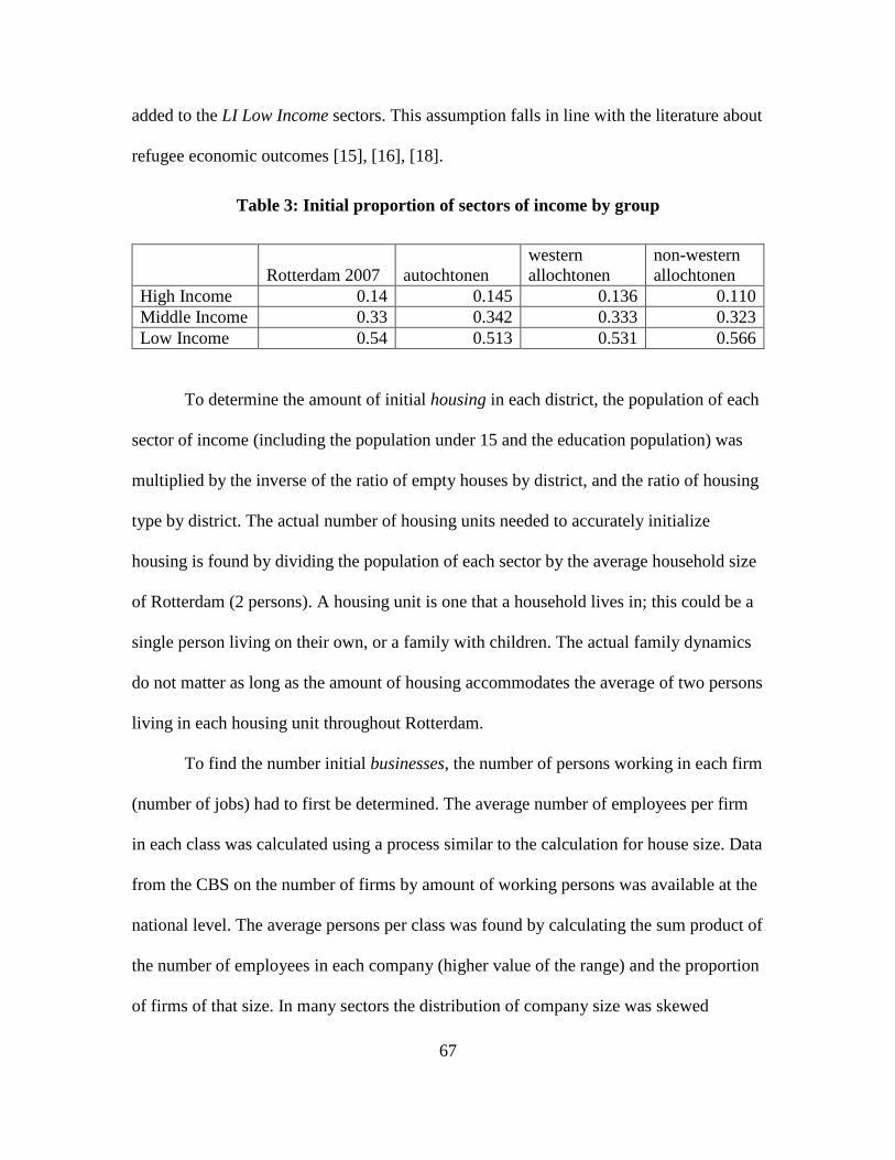
67
added to the LI Low Income sectors. This assumption falls in line with the literature about
refugee economic outcomes [15], [16], [18].
Table 3: Initial proportion of sectors of income by group
Rotterdam 2007 autochtonen western allochtonen
non-western allochtonen
High Income 0.14 0.145 0.136 0.110 Middle Income 0.33 0.342 0.333 0.323 Low Income 0.54 0.513 0.531 0.566
To determine the amount of initial housing in each district, the population of each
sector of income (including the population under 15 and the education population) was
multiplied by the inverse of the ratio of empty houses by district, and the ratio of housing
type by district. The actual number of housing units needed to accurately initialize
housing is found by dividing the population of each sector by the average household size
of Rotterdam (2 persons). A housing unit is one that a household lives in; this could be a
single person living on their own, or a family with children. The actual family dynamics
do not matter as long as the amount of housing accommodates the average of two persons
living in each housing unit throughout Rotterdam.
To find the number initial businesses, the number of persons working in each firm
(number of jobs) had to first be determined. The average number of employees per firm
in each class was calculated using a process similar to the calculation for house size. Data
from the CBS on the number of firms by amount of working persons was available at the
national level. The average persons per class was found by calculating the sum product of
the number of employees in each company (higher value of the range) and the proportion
of firms of that size. In many sectors the distribution of company size was skewed

68
towards the low end with the majority of companies in a class being single person
companies (i.e. entrepreneurs, self-employed persons). The number of initial businesses
was modeled as dependent on the average number of persons working in each sector
because the population of each district had been established and data of the ratio of
business by class was available at the district level. A low estimate of employees per
company would give an amount of businesses that would not fit in the land area per
district. This study elected to exclude single persons from the calculation of average
persons in each business to maintain laws of conservation in the model. Table 4 shows
the calculated number of jobs per class of business as well as the number of jobs per class
of business by sector of income. The average city wide distribution of sectors of income
was used to divide the jobs accordingly and maintain a common number of jobs per firm
across all districts.
Table 4: Jobs per class by sector of income
Class Total jobs High Income Jobs Middle Income Jobs Low Income Jobs A 5.3 0.7 1.9 2.7 B-F 21.9 3.2 7.8 10.0 G+I 11.9 1.7 4.2 5.9 H+J 18.4 2.7 6.5 9.2 K-L 10.3 1.5 3.6 5.1 M-N 15.9 2.3 5.6 8.0 R-U 10.8 1.6 3.8 5.4
The initial number of business establishments was set by multiplying 2007 values
of businesses in each district by a scaling factor (while maintaining the ratio of business
classes in each district) until the total district working population had employment of
95% to match the 2007 national unemployment rate of 5% [49]. Using the 2007 ratio of

69
business classes maintained the distributions of economic activities throughout the city of
Rotterdam, while the scaling factor adjusted the number of business establishments to
accommodate the number of people in each district. The non-commuting assumption
means that persons were initially overrepresented or underrepresented in some districts in
classes of businesses. For example, in the district of Hillegersberg-Schiebroek the
proportion of high income persons is 0.28, the highest of any district in Rotterdam. The
number of jobs per class is calculated using the city-wide average ratios firms per sector.
The agriculture industry ratio of 0.056 puts 11 persons of the high income sector into that
class while the ratio of agriculture, forestry, and fishing firms in Hillegersberg-
Schiebroek of 0.00357 supplies 6.4 high income jobs. This sets the initial high income to
job ratio in Hillegersberg-Schiebroek for agriculture, forestry, and fishing at 1.7. There
are other instances where the job ratio is as low as 0.5. This is the result of the non-
commuting assumption and the assumption that persons are equally represented in each
industry according to jobs per class.
The impact of this initialization is an initial drop in the UDRI model working
population of the city as some persons leave undesirable areas and move to more
desirable areas. After a short break-in period, the model city population begins to grow at
a rate similar to one that is seen in Rotterdam [49]. Figure 7 shows the population of the
city over the first seven years of the simulation.
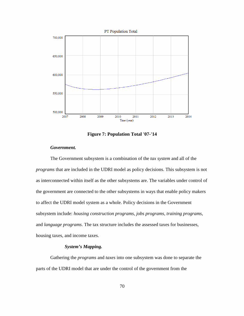
70
Figure 7: Population Total '07-'14
Government.
The Government subsystem is a combination of the tax system and all of the
programs that are included in the UDRI model as policy decisions. This subsystem is not
as interconnected within itself as the other subsystems are. The variables under control of
the government are connected to the other subsystems in ways that enable policy makers
to affect the UDRI model system as a whole. Policy decisions in the Government
subsystem include: housing construction programs, jobs programs, training programs,
and language programs. The tax structure includes the assessed taxes for businesses,
housing taxes, and income taxes.
System’s Mapping.
Gathering the programs and taxes into one subsystem was done to separate the
parts of the UDRI model that are under the control of the government from the

71
autonomous variables that interact according to the specified decision rules. Each
program uses the subscript i; some of the programs add the subscript group for policy
that can vary across ethnic groups. This system has face validity because the programs
that are included are those that are potentially controllable factors.
The UDRI model does not represent the mechanisms by which the government
would approach the implementation of each program. The program rates are results (e.g.
jobs, houses) that are added to the appropriate level variables in addition to the normal
amounts that change according to the autonomous processes in each subsystem.
Quantitative Modeling.
The three-tiered Job Market fits well with the progressive tax system in the
Netherlands. Taxes are assessed at a higher rate for those in higher income groups. The
taxes assessed for a person in each sector of the economy was found by using the CBS
defined cutoffs for earnings in each of the sectors and Organization for Economic Co-
operation and Development (OECD) tax rates for the Netherlands [59]. The tax revenue
per person averaged over seven years (2007 to 2014) is used in the UDRI model to
provide the taxes assessed for persons from each sector of the Job Market. The OECD
also provided the tax per capita at the Dutch national level [59].
There was no publicly available data on the business taxes assessed per firm in
each class of activity. For this reason the tax revenue from each business firm was set at
the same value of 300 thousand euros per firm. This value is the same that is used by
Sanders for New Enterprise (in Sanders it was 300 thousand dollars). If more information
were available about the business taxes assessed per firm, this variable could be updated.

72
CBS data was available for the average house value for the city of Rotterdam. The
values were not available by housing type or by sector of income. The ratios of housing
assessed values for each sector were maintained according to the Sanders model and were
multiplied by 5% of average house value of Rotterdam.
These numerical values themselves do not necessarily represent the actual taxes in
the city of Rotterdam. The tax multipliers that are used in this study are influenced by the
ratio persons in sectors of income. For the purposes of the UDRI model, the relative tax
amounts between sectors is the most important aspect.
People.
The People subsystem is a collection of all of the variables that pertain to people
within the system. The variables in the People subsystem include working population,
education population and births. These variables are those that regulate the natural
population growth of the city. As the population increases the births increases, people
flow into the birthed children variable, which in turn flow into the education system.
Other variables in the People subsystem include family size, birth rate, youth
arrival rate, as well as immigrant arrival rates and job sector ratios. Youth arrival rate is
a variable that is used to separate the persons who are under the age of 18 (thus under
compulsory education laws) into the Education subsystem. Figure 8 shows the
organization of some of the variables in the People subsystem.

73
Figure 8: People Subsystem
System’s Mapping.
The People subsystem has face validity because it is a simple flow of the
populations of persons. This subsystem is similar to other population models in the way
that the increase in population positively affects the birth rate. The UDRI model separates
people into a working and education population because it is assumed that persons who
are in the education system do not make decisions about where they will move. This is
because the majority of persons who are in the education system are under the age of 18
and would be assumed to be living with parents or guardians. Persons over the age of 18
in the education system are not necessarily influenced by the Job Market in their district.
Quantitative Modeling.
The birth rate was determined using the Rotterdam net birth ratio (births per 1000
people less deaths per 1000 people). It was hypothesized that the birth rates were not the
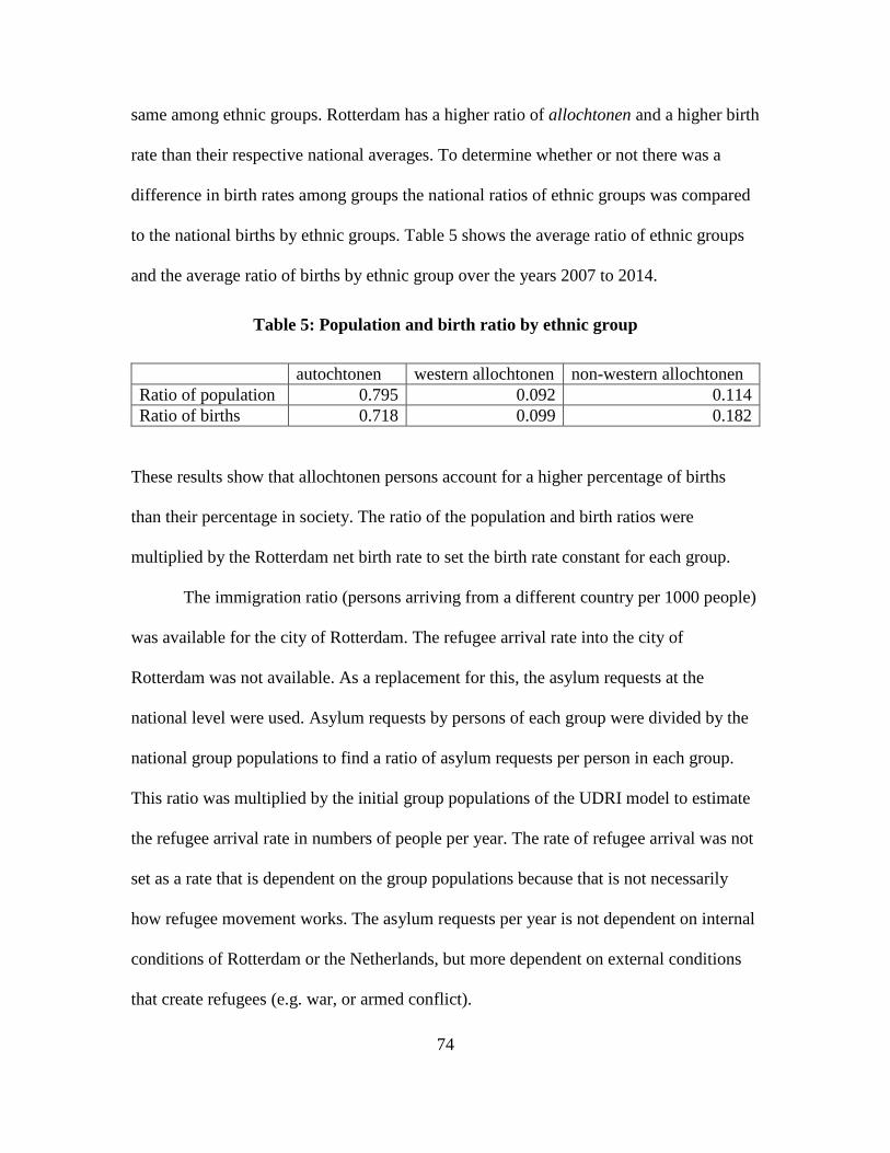
74
same among ethnic groups. Rotterdam has a higher ratio of allochtonen and a higher birth
rate than their respective national averages. To determine whether or not there was a
difference in birth rates among groups the national ratios of ethnic groups was compared
to the national births by ethnic groups. Table 5 shows the average ratio of ethnic groups
and the average ratio of births by ethnic group over the years 2007 to 2014.
Table 5: Population and birth ratio by ethnic group
autochtonen western allochtonen non-western allochtonen Ratio of population 0.795 0.092 0.114 Ratio of births 0.718 0.099 0.182
These results show that allochtonen persons account for a higher percentage of births
than their percentage in society. The ratio of the population and birth ratios were
multiplied by the Rotterdam net birth rate to set the birth rate constant for each group.
The immigration ratio (persons arriving from a different country per 1000 people)
was available for the city of Rotterdam. The refugee arrival rate into the city of
Rotterdam was not available. As a replacement for this, the asylum requests at the
national level were used. Asylum requests by persons of each group were divided by the
national group populations to find a ratio of asylum requests per person in each group.
This ratio was multiplied by the initial group populations of the UDRI model to estimate
the refugee arrival rate in numbers of people per year. The rate of refugee arrival was not
set as a rate that is dependent on the group populations because that is not necessarily
how refugee movement works. The asylum requests per year is not dependent on internal
conditions of Rotterdam or the Netherlands, but more dependent on external conditions
that create refugees (e.g. war, or armed conflict).

75
Legal.
The Legal subsystem is a representation of the Dutch integration program. The
subsystem includes variables for new migrants (both refugees and immigrants) arriving to
the city, as well as the levels for people who are in the integration period and in various
stages of the integration system. People enter and transition to one of three places:
integration exam, NT2, or exempt. From there, persons proceed into the naturalization
process or permanent residency. People who do not pass the exam retake the test and a
small proportion exit the city system. Figure 9 shows the structure of the Legal
subsystem.
Refugees are the amount of people who have entered the city after being granted
asylum from the government of the Netherlands and their children. Immigrants are those
who migrate from other countries into the Netherlands and then subsequently enter the
city. These are different from persons who are of the same ethnic group but are already
Dutch citizens. This is an important distinction because the persons of each group who
migrate in and out of the city freely according to housing and economic indicators are
Dutch citizens. The immigrants from each group may exit the city through the Legal
subsystem; these arrivals and exits (by i and group) are still tracked within the People
subsystem.
This subsystem is a parallel structure to the People, Job Market, and Land Use.
This is because the levels of the amount of people arriving into the Legal system
(according to subscripts i and group) is equivalent to the amount of immigrants and
refugees entering the city (also according to subscripts i and group). The only exception
to this is the autochtonen group; persons whose parents are both of Dutch origin are not
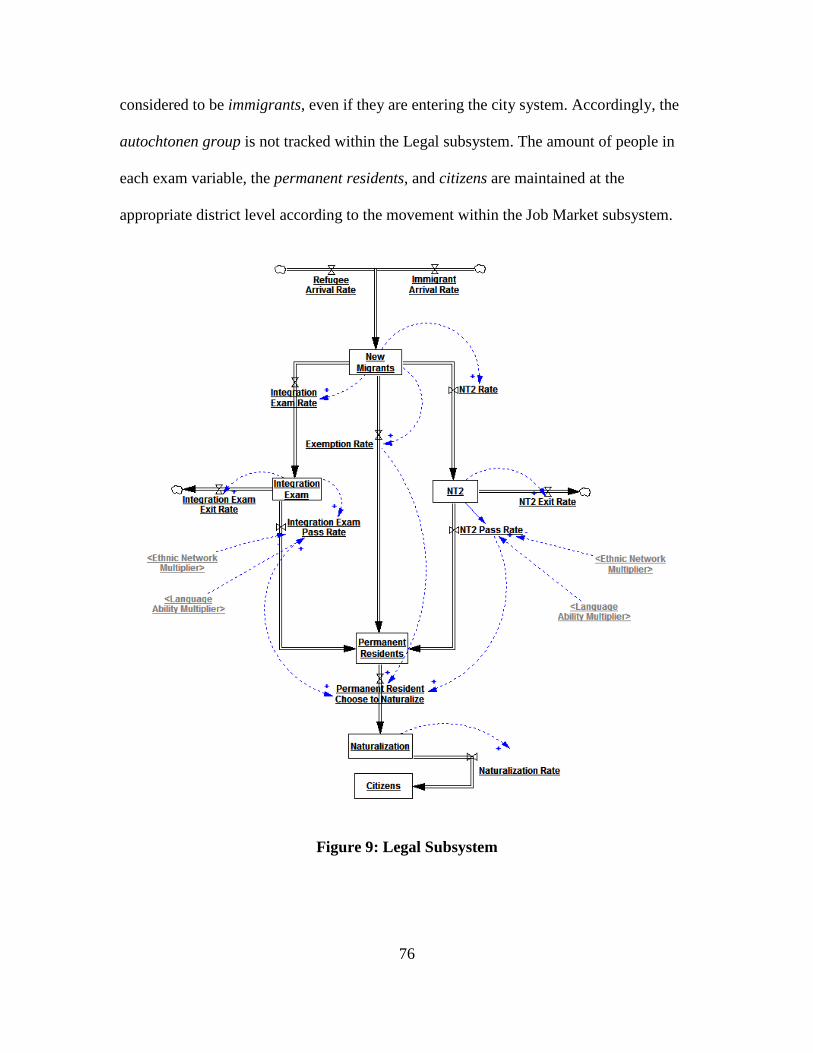
76
considered to be immigrants, even if they are entering the city system. Accordingly, the
autochtonen group is not tracked within the Legal subsystem. The amount of people in
each exam variable, the permanent residents, and citizens are maintained at the
appropriate district level according to the movement within the Job Market subsystem.
Figure 9: Legal Subsystem
77
System’s Mapping.
This system structure was developed using information from the Dutch
Immigration and Naturalization Service (IND) websites [33], [34]. According to Dutch
integration policy in effect at this time, all newly-arrived immigrants are subject to the
completion of either the Civic Integration Exam or the NT2, or they must be exempt from
taking it according to specific criteria. Exemption criteria includes those who have a
degree from a school that was taught in Dutch language and illiterate persons. Once
persons become permanent residents they have the option to choose to naturalize and
become a citizen.
Quantitative Modeling.
The NT2 is an exam that is taken by individuals who seek to pursue higher
education or obtain employment certifications in a higher-skill career field. The rate that
people elect to take the NT2 is set as the group rate constant for individuals entering
higher education; the two rates are the same because the type of people who take the NT2
and enter higher education have the same intentions so the higher education rate was used
to set the NT2 rate. Information of the success rate for individuals taking the exam was
found in reports on the NT2 exam from the Dutch Ministry of Education, Culture, and
Science (OCW) [60], [61]. The reported 2007 overall passing rate of 61.5% was used as
the NT2 Pass Rate constant.
There was no public information available about the rate that people elect to take
the Civic Integration Exam or the rate that people who take the exam pass it. The NT2
requires a more advanced mastery of the Dutch language than the Civic Integration exam.
This might mean that the passing rate for the Civic Integration Exam would be higher

78
than that of the NT2. However, persons who are taking the NT2 are likely more skilled in
the Dutch language than those who elect to take the Civic Integration Exam. It is for this
reason that the Civic Integration Exam passing rate constant was set as the same value as
the NT2 passing rate constant. The rate that people take the Civic Integration Exam is
equivalent to the rate that persons choose to attend vocational schools; the NT2 rate and
Civic Integration Exam rate comprise almost all of the proportion of people entering the
Legal subsystem. The remaining people (approximately 1%) is the rate that people are
exempt from taking either exam.
The rate that persons choose to naturalize was determined from CBS national
level data on the number of naturalizations per immigrant. The rate is assumed to be a
constant 2.9% of persons who pass each exam (or are exempt). The rate that persons are
denied a residency permit after failing to complete the integration requirements is not
publically available. This rate was assumed to be minimal so each test was assigned an
exit rate of 0.5% of persons leaving per time period.
Education.
The Education subsystem is a representation of the school system in the
Netherlands. The Netherlands education system is administered by the Dutch Ministry of
Education, Culture, and Science (OCW). Youth in the Netherlands generally enter
education at the age of 4 [62]. Then, the majority of student progress through mainstream
primary education (BAO) which lasts 8 years; a small proportion of students attend
special education (SO) or special primary education (SBAO) during this time period [62].
Students who attended special education (SO) or special primary education (SBAO)

79
proceed to elementary vocational training (PRO) or secondary special education (VSO)
[62]. Figure 10 illustrates this flow as it exists in the UDRI model.
Figure 10: Primary education and transitional secondary education
At the end of primary education (BAO) students take a test (known as Citotest or
Cito-toets) that recommends the route they should take in secondary education (VO) [62].
Secondary education (VO) lasts two years and helps student transition into their particular
focus-area; students can either select to focus on academic or vocational education.
Students entering pre-vocational secondary education (VMBO) are those who prefer (or
were recommended) to learn skills and knowledge as they apply to a particular vocation
[62]; pre-vocational secondary education lasts for two years. Academic secondary
education is divided into two tracks: pre-university education (VWO) and general
secondary education (HAVO) [62]. These tracks are tailored towards the two different
types of tertiary education. Pre-university education (VWO) lasts four years and is

80
intended to prepare students for academic higher education (WO); academic higher
education (WO) institutions are universities that focus on research and theoretical
application of knowledge [62]. General secondary education (HAVO) lasts for three years
and is expected to prepare students for professional higher education (HBO): education
that is more focused on practical applications of knowledge in a particular field [62].
Students can transfer between different programs during their secondary education
depending on qualification and availability [62]. Figure 11 shows the levels of secondary
education as they are represented in the UDRI model.
Beyond pre-vocational secondary education (VMBO) there are four levels of
vocational education (MBO) [62]. The four levels of vocational education (MBO) are
denoted by numbers (e.g. MBO 2). Each level lasts a different length and teaches
different types of vocational skills. MBO 1 is focused on simple executive tasks; MBO 4
teach middle-management skills and graduates have the ability to enter professional
higher education (HBO) should they choose to.
Figure 11: Secondary education

81
System’s Mapping.
The Education subsystem structure is developed directly from OCW [62]–[64]
and OECD [65] reports. These reports describe the flow of students between levels of the
education system as well as average dropout and graduation rates. The representation of
Dutch education in the UDRI model is accurate for the time horizon of this study; all of
the OCW reports [62]–[64] show the same school structure and there have been no
changes made to the system structure since the publication of the most recent (2013)
report found. Each level of education includes the subscripts i and group. The structure of
the Education subsystem is intuitively linked to the Job Market; for example, individuals
who dropout of education before they have basic qualifications (according to OCW) will
enter the Low Income sector. Figure 12 shows the full Education subsystem to provide
perspective on the flow between the previously shown Education figures.
As persons move throughout the city, a proportional amount of persons in the
same ethnic group move with them. The persons in the education system that move are
those who are under the age of 18. This education system assumes that persons in
secondary education or lower are those who live with parents or guardians and therefore
move in proportion to movements in the Job Market.
This education system assumes that students flow through each level with
dropouts occurring in the last year of each level (before students move on to the next
level). This is because there was data available on dropout rates from each level of
education, but not on the year that people drop out. The UDRI model makes the
optimistic assumption that each student is given the best opportunity to succeed at each
level before they dropout.
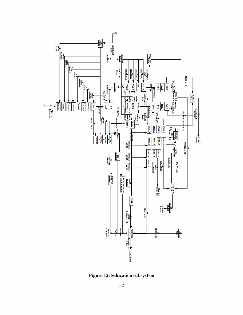
82
Figure 12: Education subsystem

83
Quantitative Modeling.
This subsystem was quantitatively validated in isolation prior to connecting it to
the other subsystems in the UDRI model. This quantitative validation was done by using
a constant population of 100 students entering the system. A constant inflow of students
allowed for direct comparison to outflow; determining the percentage (number of persons
per 100) of qualified and unqualified students exiting the system from each year group
that entered would not be possible with an increasing population. Rate constants for
transition between education levels were set according to the OCW report [62, Fig. 2.1].
These numbers are averages across the Netherlands education system. Identical outflows
of percentage of students from each of the levels of education confirmed that the
education system was quantitatively valid.
The rates for dropouts, choices of education track (between academic and
vocational), and the subjects of study were different among ethnic groups. Non-western
allochtonen had actual dropout rates two times greater than their autochtonen classmates.
Non-western allochtonen were much less likely to enter academic secondary education
(HAVO/VWO) and chose to enter vocational secondary education (VMBO). To model
this, the rates between levels of education and dropout rates were set at the average value
for autochtonen students. The rate for selection of either academic or vocational
education were multiplied by economic integration of low income persons for each group
of allochtonen. The economic integration is a variable that is explained in the Social
subsystem section.
84
Social.
The variables in the Social subsystem are created from literature that describes
social phenomena An example is Benenson’s [40] economic tension, which influences
people’s residential decisions through comparison of a person’s economic status to that of
their neighbors. Other variables in the Social subsystem that have been adapted from
literature include cognitive dissonance [40] and ethnic network multiplier [15], [20].
Another major function of the Social subsystem is to provide measures of
integration for refugees and immigrants. Integration is measured by three variables:
economic integration, legal integration, and social integration. Each of those integration
variables is comprised of variables that address different components of each aspect of
integration. The variables compare the economic, legal, and social status of each
allochtonen group to the autochtonen group. The aim of the current Dutch integration
system is to minimize the differences between immigrants and the native Dutch
population. For this reason, the integration measures in the UDRI model are ratios of
variables for each group over the same variables for autochtonen. An example of this is
the Economic integration of low income persons. The fraction of low income persons in
each group population is divided by the fraction of low income persons in the
autochtonen group population. A value greater than one indicates that, relative to their
group populations, a group has more persons of low income status; it follows that an
integration variable value less than one indicates that a group population has relatively
fewer persons of that designation. Table 6 shows the integration measures used in the
UDRI model. It should be noted that the value of each of these measures is one for the
autochtonen group because they are they baseline to which other groups are compared to.

85
These measures are used as response variables in the policy experiments conducted in the
forecasting/optimization validation section.
Table 6: Integration measures
Variable Name Formula
Social Integration Total
𝐷𝐷𝐷𝐷𝑑𝑑𝑑𝑑ℎ 𝑆𝑆𝑆𝑆𝑑𝑑𝑙𝑙𝑘𝑘𝑑𝑑𝑆𝑆𝑑𝑑𝑃𝑃𝑃𝑃𝑃𝑃 𝑃𝑃𝑃𝑃𝑆𝑆𝐷𝐷𝑙𝑙𝑙𝑙𝑑𝑑𝑑𝑑𝑃𝑃𝑙𝑙 𝑃𝑃𝑆𝑆𝑃𝑃𝐷𝐷𝑆𝑆 𝑃𝑃𝑃𝑃𝑑𝑑𝑙𝑙𝑙𝑙
Legal Integration Total
𝑃𝑃𝑑𝑑𝑆𝑆𝑘𝑘𝑙𝑙𝑙𝑙𝑑𝑑𝑙𝑙𝑑𝑑 𝐴𝐴𝑑𝑑𝑑𝑑𝑑𝑑𝑙𝑙𝑑𝑑𝑙𝑙𝑑𝑑𝑑𝑑 + 𝑁𝑁𝑙𝑙𝑑𝑑𝐷𝐷𝑆𝑆𝑙𝑙𝑙𝑙𝑑𝑑𝑁𝑁𝑙𝑙𝑑𝑑𝑑𝑑𝑃𝑃𝑙𝑙 + 𝐶𝐶𝑑𝑑𝑑𝑑𝑑𝑑𝑁𝑁𝑑𝑑𝑙𝑙𝑑𝑑𝑃𝑃𝑃𝑃𝑃𝑃 𝑃𝑃𝑃𝑃𝑆𝑆𝐷𝐷𝑙𝑙𝑙𝑙𝑑𝑑𝑑𝑑𝑃𝑃𝑙𝑙 𝑃𝑃𝑆𝑆𝑃𝑃𝐷𝐷𝑆𝑆 𝑃𝑃𝑃𝑃𝑑𝑑𝑙𝑙𝑙𝑙
Economic Integration Low Income
𝐹𝐹𝑆𝑆𝑙𝑙𝑑𝑑𝑑𝑑𝑑𝑑𝑃𝑃𝑙𝑙 𝐿𝐿𝐿𝐿 𝑃𝑃𝑜𝑜 𝑃𝑃𝑆𝑆𝑃𝑃𝐷𝐷𝑆𝑆 𝑊𝑊𝑃𝑃𝑆𝑆𝑘𝑘𝑑𝑑𝑙𝑙𝑊𝑊 𝑃𝑃𝑃𝑃𝑆𝑆𝐷𝐷𝑙𝑙𝑙𝑙𝑑𝑑𝑑𝑑𝑃𝑃𝑙𝑙 [𝑊𝑊𝑆𝑆𝑃𝑃𝐷𝐷𝑆𝑆]𝐹𝐹𝑆𝑆𝑙𝑙𝑑𝑑𝑑𝑑𝑑𝑑𝑃𝑃𝑙𝑙 𝐿𝐿𝐿𝐿 𝑃𝑃𝑜𝑜 𝑃𝑃𝑆𝑆𝑃𝑃𝐷𝐷𝑆𝑆 𝑊𝑊𝑃𝑃𝑆𝑆𝑘𝑘𝑑𝑑𝑙𝑙𝑊𝑊 𝑃𝑃𝑃𝑃𝑆𝑆𝐷𝐷𝑙𝑙𝑙𝑙𝑑𝑑𝑑𝑑𝑃𝑃𝑙𝑙 [𝑙𝑙𝐷𝐷𝑑𝑑𝑃𝑃𝑑𝑑ℎ𝑑𝑑𝑃𝑃𝑙𝑙𝑑𝑑𝑙𝑙]
Economic Integration Middle Income
𝐹𝐹𝑆𝑆𝑙𝑙𝑑𝑑𝑑𝑑𝑑𝑑𝑃𝑃𝑙𝑙 𝑀𝑀𝐿𝐿 𝑃𝑃𝑜𝑜 𝑃𝑃𝑆𝑆𝑃𝑃𝐷𝐷𝑆𝑆 𝑊𝑊𝑃𝑃𝑆𝑆𝑘𝑘𝑑𝑑𝑙𝑙𝑊𝑊 𝑃𝑃𝑃𝑃𝑆𝑆𝐷𝐷𝑙𝑙𝑙𝑙𝑑𝑑𝑑𝑑𝑃𝑃𝑙𝑙 [𝑊𝑊𝑆𝑆𝑃𝑃𝐷𝐷𝑆𝑆]𝐹𝐹𝑆𝑆𝑙𝑙𝑑𝑑𝑑𝑑𝑑𝑑𝑃𝑃𝑙𝑙 𝑀𝑀𝐿𝐿 𝑃𝑃𝑜𝑜 𝑃𝑃𝑆𝑆𝑃𝑃𝐷𝐷𝑆𝑆 𝑊𝑊𝑃𝑃𝑆𝑆𝑘𝑘𝑑𝑑𝑙𝑙𝑊𝑊 𝑃𝑃𝑃𝑃𝑆𝑆𝐷𝐷𝑙𝑙𝑙𝑙𝑑𝑑𝑑𝑑𝑃𝑃𝑙𝑙 [𝑙𝑙𝐷𝐷𝑑𝑑𝑃𝑃𝑑𝑑ℎ𝑑𝑑𝑃𝑃𝑙𝑙𝑑𝑑𝑙𝑙]
Economic Integration High Income
𝐹𝐹𝑆𝑆𝑙𝑙𝑑𝑑𝑑𝑑𝑑𝑑𝑃𝑃𝑙𝑙 𝐻𝐻𝐿𝐿 𝑃𝑃𝑜𝑜 𝑃𝑃𝑆𝑆𝑃𝑃𝐷𝐷𝑆𝑆 𝑊𝑊𝑃𝑃𝑆𝑆𝑘𝑘𝑑𝑑𝑙𝑙𝑊𝑊 𝑃𝑃𝑃𝑃𝑆𝑆𝐷𝐷𝑙𝑙𝑙𝑙𝑑𝑑𝑑𝑑𝑃𝑃𝑙𝑙 [𝑊𝑊𝑆𝑆𝑃𝑃𝐷𝐷𝑆𝑆]𝐹𝐹𝑆𝑆𝑙𝑙𝑑𝑑𝑑𝑑𝑑𝑑𝑃𝑃𝑙𝑙 𝐻𝐻𝐿𝐿 𝑃𝑃𝑜𝑜 𝑃𝑃𝑆𝑆𝑃𝑃𝐷𝐷𝑆𝑆 𝑊𝑊𝑃𝑃𝑆𝑆𝑘𝑘𝑑𝑑𝑙𝑙𝑊𝑊 𝑃𝑃𝑃𝑃𝑆𝑆𝐷𝐷𝑙𝑙𝑙𝑙𝑑𝑑𝑑𝑑𝑃𝑃𝑙𝑙 [𝑙𝑙𝐷𝐷𝑑𝑑𝑃𝑃𝑑𝑑ℎ𝑑𝑑𝑃𝑃𝑙𝑙𝑑𝑑𝑙𝑙]
Similarity is used to measure integration because of the Dutch integration policy
focus, but also because of the social impacts of differences between populations.
Refugees who are markedly different from the majority in terms of culture, ethnicity, and
lower economic status are more ‘visible’ to native persons in their host nation [11], [35].
High visibility (i.e. visibly different) refugees are likely to reinforce public perception of
asylum seekers being a burden on society: whether or not this is the actual truth [11].
Refugees who are not able to achieve equitable outcomes (high unemployment and low
economic status relative to host population) are likely to become frustrated and develop
negative feelings towards the host nation population [11]. The UDRI model does not
include a measure for the sentiment of refugees; however, the trend in the integration
variables provide insight into the experiences of different groups within the model.

86
System’s Mapping.
The Social subsystem of the UDRI model is not truly a structured subsystem, but
a collection of variable functions that inform other parts of the model; in this way, it is
similar to the Government and People subsystems. The existence of social variables that
influence other parts of the UDRI model is supported by literature. The social variables
that are used to influence other parts of the UDRI model and have not been previously
been discussed are: Language Labor Multiplier, Language Ability Multiplier, and Ethnic
Network Multiplier. The Language Labor Multiplier and Language Ability Multiplier are
described in detail in the following quantitative modeling section of this subsystem. The
Ethnic Network Multiplier is a variable that incorporates ethnic concentration to change
the integration exams passing rates as well as the rate for persons moving from the low
income sector to the middle income sector. This multiplier decreases all of these rates as
the group population ratio in each district increases. Numerous studies (discussed in the
literature review chapter) identify high ethnic concentration as factor that influences
integration outcomes. As the Ethnic Network Multiplier increases, the passing rate for
integration exams decreases. This is because high ethnic concentration is detrimental to
the language ability of ethnic groups [18]. The Ethnic Network Multiplier decreases the
rate that persons move from low income to middle income within a district. This is
because a high concentration of co-ethnic individuals within a district has a positive
impact on employment, but only within the district [15], [20]; therefore there is an
increase in the unemployment of persons of minority ethnic groups because of increases
competition for the available jobs within the ethnic network. Table 7 shows the uses of
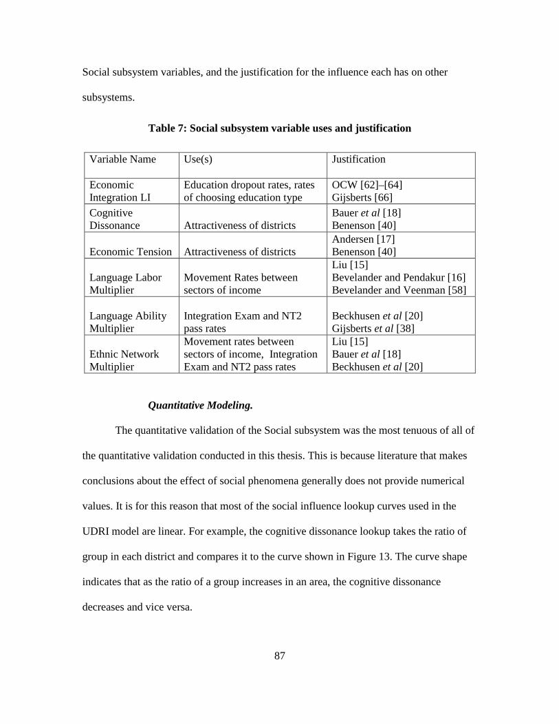
87
Social subsystem variables, and the justification for the influence each has on other
subsystems.
Table 7: Social subsystem variable uses and justification
Variable Name Use(s) Justification
Economic Integration LI
Education dropout rates, rates of choosing education type
OCW [62]–[64] Gijsberts [66]
Cognitive Dissonance Attractiveness of districts
Bauer et al [18] Benenson [40]
Economic Tension Attractiveness of districts Andersen [17] Benenson [40]
Language Labor Multiplier
Movement Rates between sectors of income
Liu [15] Bevelander and Pendakur [16] Bevelander and Veenman [58]
Language Ability Multiplier
Integration Exam and NT2 pass rates
Beckhusen et al [20] Gijsberts et al [38]
Ethnic Network Multiplier
Movement rates between sectors of income, Integration Exam and NT2 pass rates
Liu [15] Bauer et al [18] Beckhusen et al [20]
Quantitative Modeling.
The quantitative validation of the Social subsystem was the most tenuous of all of
the quantitative validation conducted in this thesis. This is because literature that makes
conclusions about the effect of social phenomena generally does not provide numerical
values. It is for this reason that most of the social influence lookup curves used in the
UDRI model are linear. For example, the cognitive dissonance lookup takes the ratio of
group in each district and compares it to the curve shown in Figure 13. The curve shape
indicates that as the ratio of a group increases in an area, the cognitive dissonance
decreases and vice versa.

88
Figure 13: Cognitive dissonance lookup curve
The only non-linear curve unique to this thesis is the lookup curve that is used to
determine the language labor multiplier and the language ability multiplier. This curve
inputs the ratio of Dutch speakers and outputs a multiplier. As the ratio of Dutch speakers
in each district by group increases the language labor multiplier increases; the language
labor multiplier impacts the flow of groups from low income to middle income and from
middle income to high income. The s-curve (shown in Figure 14) indicates that as the
ratio of Dutch speakers increases, the rate that persons are able to move upwards through
the sectors of income increases. There is a decreasing marginal effect of additional Dutch
speakers as the ratio approaches one.
The language labor multiplier is based upon economic outcomes literature that
notes the importance of language ability for individuals to gain employment and
economic advancement.

89
Figure 14: Language multiplier s-curve
The language ability multiplier uses the ratio of Dutch speakers in the entire
district to influence the rate that persons pass the Civic Integration Exam and NT2. This
multiplier uses the Dutch speakers of all groups in the district because as the amount of
persons who speak Dutch increases, the more that people who live in the district are
exposed to the Dutch language. This increased exposure is assumed to have a positive
effect on the language skills of immigrants and refugees in the integration system.
Model Validation
System’s Mapping.
When conducting system’s mapping validation of the UDRI model, as a whole,
the focus is on the way the subsystems are interconnected. The decision rules must be
examined to determine if the system as a whole is valid. The overall flow of information
and persons in the model is shown in Figure 15.
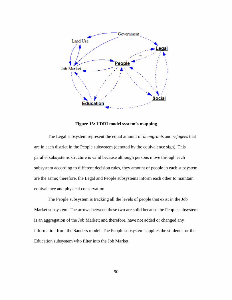
90
Figure 15: UDRI model system’s mapping
The Legal subsystem represent the equal amount of immigrants and refugees that
are in each district in the People subsystem (denoted by the equivalence sign). This
parallel subsystems structure is valid because although persons move through each
subsystem according to different decision rules, they amount of people in each subsystem
are the same; therefore, the Legal and People subsystems inform each other to maintain
equivalence and physical conservation.
The People subsystem is tracking all the levels of people that exist in the Job
Market subsystem. The arrows between these two are solid because the People subsystem
is an aggregation of the Job Market; and therefore, have not added or changed any
information from the Sanders model. The People subsystem supplies the students for the
Education subsystem who filter into the Job Market.

91
The Social subsystem contains integration measures that are informed by the
People and Legal subsystems. Social subsystem variables inform the People, Legal, and
Education subsystems. These connections are supported by literature (shown in Table 7).
Quantitative Modeling.
Part of the quantitative modeling validation has been conducted at the subsystem
level. The constants of arrival rates, and construction rates were set according to available
empirical data. Lookup curves for multipliers that were in the Sander’s model were not
modified because these describe the relative interactions between the different sectors of
the Job Market. The constants have been tailored to a particular city, so the curves will
still explain the interactions within the city that have been validated by both Forrester and
Sanders. Quantitative validation of the UDRI model as a whole included examination of
physical conservation, integration method, extreme conditions, and endogenous behavior
reproduction testing.
Simulations of early versions of the UDRI model revealed that there were
problems with maintaining physical conservation within the Education subsystem. In
some districts there were very few students in particular education levels (e.g. PRO/VSO,
especially western-allochtonen refugee students). Persons were leaving the city at such a
high rate that there were occurrences where rounding errors resulted in negative persons
being in a level. This of course is not possible. To fix the issue of conservation, checks
were added into the balance equation of each education level to ensure that the net
movement of individuals in the Job Market would only reduce the level to a minimum of
zero. It should be noted that the population of groups in the working population of each
district is greater than the group education population. Therefore, according to the UDRI

92
model assumptions, it is possible for there to be persons of an ethnic group in a district
but zero persons in levels of the education system.
The integration method was checked to ensure that using a different method
would not create errors in the model or different results. The default integration method
within Vensim uses the Euler method. The other integration option within Vensim uses a
difference method. These two methods were compared using a capability within Vensim
to compare the results of runs. Both methods produced identical results with runs that
operated under the same assumptions. This study uses the Euler method for the
experiments with the UDRI model.
Under extreme condition testing some of the variables from the Sanders’s model
initially produced errors when runs were completed using assumptions of the UDRI
model in this thesis. Variables such as MHOM MI housing obsolescence multiplier i are
calculated using the natural log of an input variable. The input variable for MHOM MI
housing obsolescence multiplier i is MHM MI housing multiplier i. As the land of a city
is used up, the housing multipliers go to zero. The natural log of zero is undefined, so a
check was established for these natural log equations that uses the maximum of the input
variable or a constant; the constant for each equation is the input that produces the lower
boundary output variable of the lookup function. This check does not affect the results of
the model runs because inputs outside the defined range of lookup curves are set at either
the highest or lowest defined input (depending on whether the input variable is above or
below the bounds, respectively).
The behavior modes that are important in this study are an increase in the
economic divide between the different ethnic groups. Figure 16 shows the comparison of
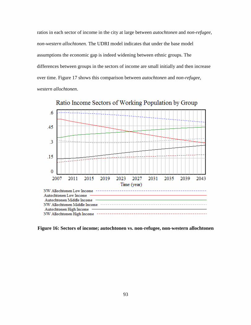
93
ratios in each sector of income in the city at large between autochtonen and non-refugee,
non-western allochtonen. The UDRI model indicates that under the base model
assumptions the economic gap is indeed widening between ethnic groups. The
differences between groups in the sectors of income are small initially and then increase
over time. Figure 17 shows this comparison between autochtonen and non-refugee,
western allochtonen.
Figure 16: Sectors of income; autochtonen vs. non-refugee, non-western allochtonen

94
Figure 17: Sectors of income; autochtonen vs. non-refugee western allochtonen
The difference in economic outcomes between refugees and autochtonen are more
extreme than those for their non-refugee counterparts. Figure 18 shows the comparison of
ratios in each sector of income in the city at large between autochtonen and non-western
allochtonen refugees; Figure 19 shows this same comparison for western allochtonen
refugees. The graphs show the same patterns that exist for non-refugee allochtonen. The
differences in economic outcomes of for refugees compared to non-refugees of the same
group can be explained by three main factors: initialization, language ability, and refugee
arrival assumptions. Each refugee group begins with no one in the high income sector
and no Dutch speakers. Language ability is important for mobility between sectors. It is
assumed that refugees arrive to the city and enter either the low income or middle income

95
sector. The non-refugee immigrants arrive in proportion to the amount of persons who are
in each sector. There is no flow from outside the system into the high income for
refugees, so all high income refugees must come from within the system through the Job
Market.
Figure 18: Sectors of income; autochtonen vs. non-western allochtonen refugee
Figure 19: Sectors of income; autochtonen vs. western allochtonen refugee

96
The results of these economic outcome graphs should be analyzed based upon the
trends they show and not for the values; in a real city the ratio of low income persons
would likely not become less than the ratio of high income persons. The trends show that
the UDRI model produces the system behavior of widening economic disparity described
in refugee studies and presented in reports from Dutch national sources.
Another mode of behavior that is of interest is the changing distribution of ethnic
groups throughout the city. Figure 20 shows the ratio of ethnic group by district for
Centrum. The ratio of non-western allochtonen persons increases over time as the ratio of
autochtonen persons decreases. The ratio of western allochtonen persons increases at a
slower rate than non-western allochtonen persons. All of the districts display a similar
trend. The ratio of group by district for each allochtonen group includes refugees. These
trends of changing ethnic group distribution are evident in the CBS data. The economic
and ethnic group modes of behavior occur at the same time so the phase of behaviors in
the UDRI model is valid according to the endogenous behaviors of interest test.
Figure 20: Ratio of group by district, Centrum
97
Hypothesis Testing.
Hypothesis testing validation for the UDRI model was comprised of policy
decision rules, and behavior sensitivity analysis. The policy decision rules in the UDRI
model capture the actions of the governmental authority. The municipal government of
Rotterdam has the authority to effect economic policy such as job creation and job
training. The municipal authorities can also regulate the classes of business activities by
allowing certain industries to expand in open areas of the city. Other programs that fall
under municipal authority include housing construction programs and language training
programs.
A policy that was not used in the UDRI model was a policy that limited the
amount of refugees or immigrants entering the city system. This study assumes that
Rotterdam does not have the ability to refuse asylum seekers if the Dutch government has
accepted their asylum application. This assumption is made because of the national
government has authority over the municipal government within the Netherlands. This
assumption would also make the analysis of the city system a trivial matter. Examining
the integration of refugees when there are no new refugees in the system is a fruitless
endeavor. This study recognizes the reality that refugee flow into cities exists and will
continue into the future. Policy analysis should be done with this reality intact to
understand the best ways to address the problem behavior modes; stopping refugees from
entering the city ignores the issues surrounding integration instead of addressing them.
Behavior sensitivity testing is focused on analyzing the system behaviors when
the assumptions about parameters in the model are changed. The focus for this testing is
the general trends in the variables over time. If varying the value of a parameter over the

98
range of reasonable values results in the disappearance of previously displayed model
behaviors (or appearance of new ones), then the model is sensitive to that parameter
value. This does not necessarily invalidate the parameter assumption. Finding sensitive
parameters provides insight into the system being studied. Policy makers should
understand that assumptions about sensitive parameters (as they exist in the real world)
should be revisited to check the confidence in these values. The behavior sensitivity
testing and uncertainty analysis was conducted using the built-in Vensim sensitivity
analysis toolset. This process is explained in the following section uncertainty analysis
section.
Uncertainty Analysis.
In a real-world system there is a degree of uncertainty that influences how
processes function. Quantitative sensitivity testing focuses on the change in numerical
results of a model when parameters are varied over the range of reasonable values. The
range of reasonable values used can be determined using data analysis or expert opinion.
For the purpose of the sensitivity testing in the UDRI model, the range of change in
constants was from 75% to 125% of the value that is used in the baseline model. The
constants used for sensitivity testing were the ones that are unique to the UDRI model,
were calculated using empirical data, and affect the rate of processes. The list of
constants used and their low, base, and high values are shown in Appendix A.
The sensitivity simulation tool within Vensim allows users to specify constants
according to different probability distributions, select the method by which to change the
constants, and choose which variables to save as output for each run of the simulation.
Probability distributions available include, uniform, normal, and triangular probability

99
distributions. The uniform distribution was used because this distribution only requires
two parameters: a minimum value and a maximum value. There wasn’t information
available on the distribution of the constants that were calculated using CBS data. For
this reason the simplest probability distribution was chosen to use for the sensitivity
simulation. If more information were available, the UDRI model could be updated to use
the appropriate probability distribution.
The options for changing the constants are the method that govern the sampling of
the probability distributions. There are four options for sampling method: univariate,
multivariate, Latin grid, and Latin hypercube. Latin grid and Latin hypercube sampling
are discussed in the following forecasting/optimization section. The univariate method
changes one constant at a time each run of the simulation while the others are held to
their value in the baseline model. The multivariate method changes all factors
simultaneously during each run of the simulation. For the purposes of the sensitivity
validation of the UDRI model, multivariate was selected as the best option; multivariate
sampling produces sensitivity results that display a wide range of possible variable results
under uncertainty.
Behavior sensitivity validation only requires the inspection of general trends of
the system. A multivariate sampling method can indicate the range of behaviors
according to the uncertainty of all of the constants used. It is not necessary to understand
which constant causes the most uncertainty at this point; the effect of specific input
variables on output variables is investigated in the experiments described in the
forecasting/optimization section. The multivariate method is appropriate for the
quantitative sensitivity of the UDRI model as well. As previously mentioned, the

100
particular values of variables in the UDRI model are not the focus, rather it is the relation
of these values to each other that is important.
The final sensitivity simulation settings are the number of simulations and the
seed number. 500 simulations was deemed sufficient to produce sensitivity results with
large variation. The number of simulations was set at this number because the effect of
individual factors was not a concern for sensitivity analysis testing; therefore, a large
number of runs was needed, but not a number of runs that was determined through
analytical means. The seed number is a value that initializes the random number stream
used to sample constants during simulations; the seed used for the sensitivity simulation
was 2007.
The graphical results of the sensitivity simulation indicate that the behavior is
relatively insensitive to uncertainty in the constants tested. Figure 21 shows the
sensitivity graphs for low income as a ratio of the each group population. There is a color
scale to indicate the confidence bounds on the values; 50% indicates that half of the
simulation runs lie within that region. The entire shaded region represents 100% of all
simulation runs. The graphs in order of top to bottom represent: autochtonen, non-
western allochtonen, and western allochtonen. Note that the autochtonen group does not
have the same vertical scale as the other two graphs.
These graphs show that the mode of behavior of a widening gap between groups
still exists, but uncertainty in the constants creates variation in the numerical results. The
ratio of low income persons under uncertainty varies by as much as 10% for each ethnic
group. However, neither allochtonen group range overlaps with the range of values for
the autochtonen group. This indicates that the numerical results for economic outcomes

101
are sensitive to uncertainty but do not change the relative values. The other sectors of
income in all groups (including refugees) display the same trends that were seen in the
baseline model and shown in Figure 16 and Figure 17.
The ethnic group distribution within districts was more sensitive to the
uncertainty of constants. Figure 22 shows the sensitivity graphs for ratio of group by
district for Centrum. The graphs from top to bottom show the groups are autochtonen,
non-western allochtonen, and western allochtonen. Again, note that these graphs do not
have the same vertical scale. The 50% interval exhibited the same trends as shown in
Figure 20; however, some of the extreme observations indicate that the ratios by group
exhibit the opposite behavior. This is most likely due to the changing birth rates and
arrival rates for immigrants and refugees.
The sensitivity of the UDRI model demonstrates that under uncertainty the modes
of behavior of a widening economic gap between ethnic groups and a redistribution of
ethnic groups throughout the city are still present; the quantitative sensitivity increases as
time passes. This makes sense, because the after the break-in period (redistribution
according to pressures present at initialization) uncertainty in the constants results in
simulation runs in which the rates carry on trends in diverging directions.

102
Figure 21: Sensitivity of ratio LI of group working population: autochtonen, non-western allochtonen, western allochtonen

103
Figure 22: Sensitivity ratio group by district, Centrum: autochtonen, non-western allochtonen, western allochtonen
104
Forecasting/Optimization
The method used to conduct forecasting and optimization validation of the UDRI
model was to use the government program rates endogenous to the model as input
variables and then analyze the impact of these policies on the measures of integration. To
narrow the focus of the experiments, two scenarios were considered: policy impact on
policy impact on refugee integration (both non-western and western allochtonen), and
non-western allochtonen integration (non-refugee and refugee combined). Each policy in
the UDRI experiments is implemented beginning in the simulation year 2015.
The impact of policy on refugees is investigated because this group is the most
socio-economic disadvantaged group and the flow of refugees is not necessarily regular;
policy recommendations for improving outcomes and integration results for these
individuals is a main focus of this study. The non-western allochtonen group is
considered because this group had the greatest difference in economic sectors at
initialization of the model; the outcomes of non-refugees and refugees from an ethnic
group are connected because there are processes within the UDRI model that are
informed by the state of the group as a whole. The experiments hypothesize that there
may be differences in the policy recommendations when different combinations of
groups are considered
A designed experiment was created to explore the two scenarios using a Latin
Hypercube, space-filling design. This design was chosen because of the large number of
policies considered. A Latin square design produces an experiment where every
combination of factor levels is tested once; an experiment with two factors (A and B) that
each have a different number of levels (A, 4 levels; B, 3 levels) would produce a design
105
with 12 runs. An experiment with more factors or more levels would result in a larger
design. With the UDRI model there are 7 programs that can each be changed by district
or group. These program rates are continuous variables; therefore, covering the design
space adequately would require at least three levels per factor (i.e. low, center, and high
points). A design testing every combination of levels for every factor with each subscript
would not be an effective approach in this preliminary study.
In a Latin hypercube design each factor has as many levels as there are runs. The
levels are spaced evenly between the lower and upper bound of each factor. This design
is able to adequately cover the design space by spreading out all factors across their
ranges. This design is still able to detect main effects and low order interactions between
factors with much fewer runs than a Latin square design. The design matrix for the Latin
hypercube experimental design was generated using the JMP space filling design tool.
For each experiment the designed experiment used a Latin hypercube design with 480
runs. The factors and responses for each experiment is shown in Appendix A.
Summary
Model validation is a significant part of the process of system dynamics
modeling. Assumptions made in the modeling process are an abstraction of the real
system; however, no model of a real-world system is perfect. It should be noted,
however, that if more accurate data is available or became available, the relationships
could be updated. The UDRI model is valid for the purpose of exploring the behavior of
city system with refugee flow and the impact of policy on integration. The city of
Rotterdam has been used as a framework for the UDRI model; it should be reiterated that

106
this city model is not a predictive model of future behavior. The important conclusions
from the experimental results should be the direction of trends and sign of coefficients of
influential variables. The experimental results are discussed in the following analysis and
results chapter.

107
V. Analysis and Results
Overview
This chapter contains the results from the two policy analysis experiments
described at the end of the model development chapter. The significant programs for
explaining variation in the integration response were found using regression of all main
effects. Results of analysis of variance (ANOVA) models for each measure of integration
are discussed in conjunction with sensitivity graphs. The sensitivity graphs (generated in
Vensim) are shown for non-western allochtonen refugees to illustrate the range of values
for each measure of integration. The y-axis of each graph shows the level of integration; a
value of one represents full integration. Values less than one indicate that there is
underrepresentation of individuals from the ethnic group in a particular measure; a value
greater than one indicates overrepresentation. The sensitivity graphs show the pre-policy
trajectory of the integration measure, indicated by a black line. Starting in the simulation
year 2015 government programs are initiated. The variability in the integration measures
over time is indicated by the shaded bands. The integration of non-western allochtonen
refugees is shown throughout this chapter to maintain consistency and allow for the
comparison of results between experiments.
Results and Discussion
Experiment 1: Refugee Focus.
The first experiment used policy only directed towards the two refugee groups.
The impacts of government programs differ between the measures of integration. Social
integration is most affected by the learning rate of language programs. ANOVA with

108
language program rate [nw-allochtonen refugee] as the only variable results in a
significant model (i.e., F-Ratio = 22621.07, p-value <0.0001) with an R-square value of
0.979. These results are intuitive. The social integration measure is equivalent to the city-
wide language ability of each group; therefore, an increase in the language training
program causes an increase in Dutch speakers and social integration. Figure 23 shows the
first experiment sensitivity graph of social integration for non-western refugees. The
range of values for social integration of each group are higher than the base model (that
had no programs implemented).
Figure 23: Experiment 1 social integration sensitivity graph, non-western allochtonen refugees
The effect of government programs on the legal integration of refugees is more
complicated. ANOVA with legal integration indicates that a model with language
program rate [nw-allochtonen refugee], low income housing construction rate [i] (D5,
D6, D8, D10, D11), and middle income housing construction rate [i] (D5, D6, D10, D11)
results in a significant model (i.e., F-Ratio = 479.53, p-value < 0.0001) with and R-
square of 0.911. Low income housing construction in districts such as Hillegersberg-

109
Schiebroek and Kranlingen-Crooswijk creates opportunities for low income individuals
to move there. Refugees who move outside of districts with a high concentration of co-
ethnic persons are able to escape the isolating effects of the ethnic network multiplier.
Language programs coupled with the diminished ethnic network effect results in an
increased language ability and therefore an increased rate of refugees who are able to
complete their integration requirements and legally integrate. There effects of middle
income housing construction on legal integration are negative. As land is being occupied
by middle income housing, there is less area in these districts for low income individuals.
The low income individuals do not have as much opportunity to leave their district and
cannot gain from the benefit of leaving the ethnic network. Figure 24 shows the first
experiment legal integration of non-western allochtonen refugees. Note that information
about the legal status of individuals according to ethnic group was not publically
available. The legal integration measure shows a decreasing trend at the beginning of the
model simulation. This is due to a model burn-in period; therefore, the reversal of this
trend is not directly due to policy implementation in the model.
The economic integration of refugees was the most quantitatively sensitive to
policy program rates. Significant factors for explaining variation in economic integration
were the labor training programs. ANOVA with economic integration of middle income
persons indicates that a model with low income training rate [nw-allochtonen refugee],
middle income training rate [nw-allochtonen refugee], low income training rate [nw-
allochtonen refugee] squared, and the product of low income training rate [nw-
allochtonen refugee] and middle income training rate [nw-allochtonen refugee] results in

110
a significant model (i.e., F-Ratio = 16809.75, p-value < 0.0001) with an R-square of
0.993.
Figure 24: Experiment 1 legal integration sensitivity graph, non-western allochtonen refugees
The labor training programs directly increases the amount of people who move up
in socio-economic status; therefore, the effect of low income training rate [nw-
allochtonen refugee] is intuitively positive. The effect of middle income training rate
[nw-allochtonen refugee] is negative because as people leave the middle income sector
and go to the high income sector, the ratio of middle income relative to the group
population decreases. The estimated effect of Low income training rate [nw-allochtonen
refugee] squared is negative because as people leave the low income sector, there are
fewer people in the low income sector to move into the middle income sector. The
interaction effect between programs indicates that as the rate of low income persons
entering the middle income sector increases, there population of middle income persons
increases; the larger population of middle income individuals results in an increase in the
amount of people who will leave middle income. The effects of policy on economic
integration for low income and middle income non-western allochtonen refugees are
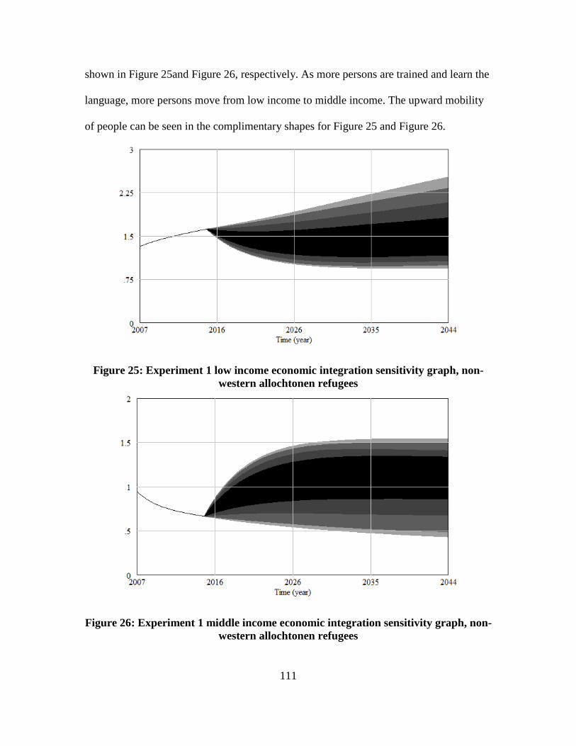
111
shown in Figure 25and Figure 26, respectively. As more persons are trained and learn the
language, more persons move from low income to middle income. The upward mobility
of people can be seen in the complimentary shapes for Figure 25 and Figure 26.
Figure 25: Experiment 1 low income economic integration sensitivity graph, non-western allochtonen refugees
Figure 26: Experiment 1 middle income economic integration sensitivity graph, non-western allochtonen refugees

112
Experiment 2: Non-western Allochtonen Focus.
The second experiment used policy that was directed towards both refugee and
non-refugee non-western allochtonen. To compare the results from experiment 1, the
same measures of integration for non-western allochtonen refugees are shown in figures
throughout this section.
The social integration of non-western allochtonen refugees in experiment 2
approximately follows the same trajectory as the social integration in experiment 1.
ANOVA with language program rate [nw-allochtonen refugee], language program rate
[nw-allochtonen], low income training rate [nw-allochtonen refugee], and low income
training rate [nw-allochtonen] results in a significant model (i.e., F-Ratio = 199.32, p-
value < 0.001) with an R-square of 0.455. Figure 27 shows the second experiment social
integration sensitivity graph for non-western allochtonen refugees. Note that Figure 23
and Figure 27 have different scales on the y-axis.
Figure 27: Experiment 2 social integration sensitivity graph, non-western allochtonen refugees

113
The effect of government policy on the legal integration of refugees in experiment
1 was minimal. Figure 24 indicates that there is not much variation in legal integration of
non-western allochtonen refugees with the implementation of policy directed towards
refugees. In the second experiment, the legal integration of the non-western allochtonen
refugees is more responsive to government programs. Figure 28 shows the variation in
legal integration. ANOVA with low income training rate [nw-allochtonen refugee], low
income training rate [nw-allochtonen], middle income training rate [nw-allochtonen
refugee], and middle income training rate [nw-allochtonen] results in a significant model
(i.e. F-Ratio = 189.39, p-value < 0.0001) with an R-square of 0.442. The difference in
the effects between experiments can be explained by the influence of the non-refugee,
non-western allochtonen population. The population of non-refugee, non-western
allochtonen is much large in magnitude than the refugee population for the same ethnic
group. For this reason, implementing programs for non-refugee individuals creates other
behaviors in the model that are not explained by the ANOVA model.
Figure 28: Experiment 2 legal integration sensitivity graph, non-western allochtonen refugees
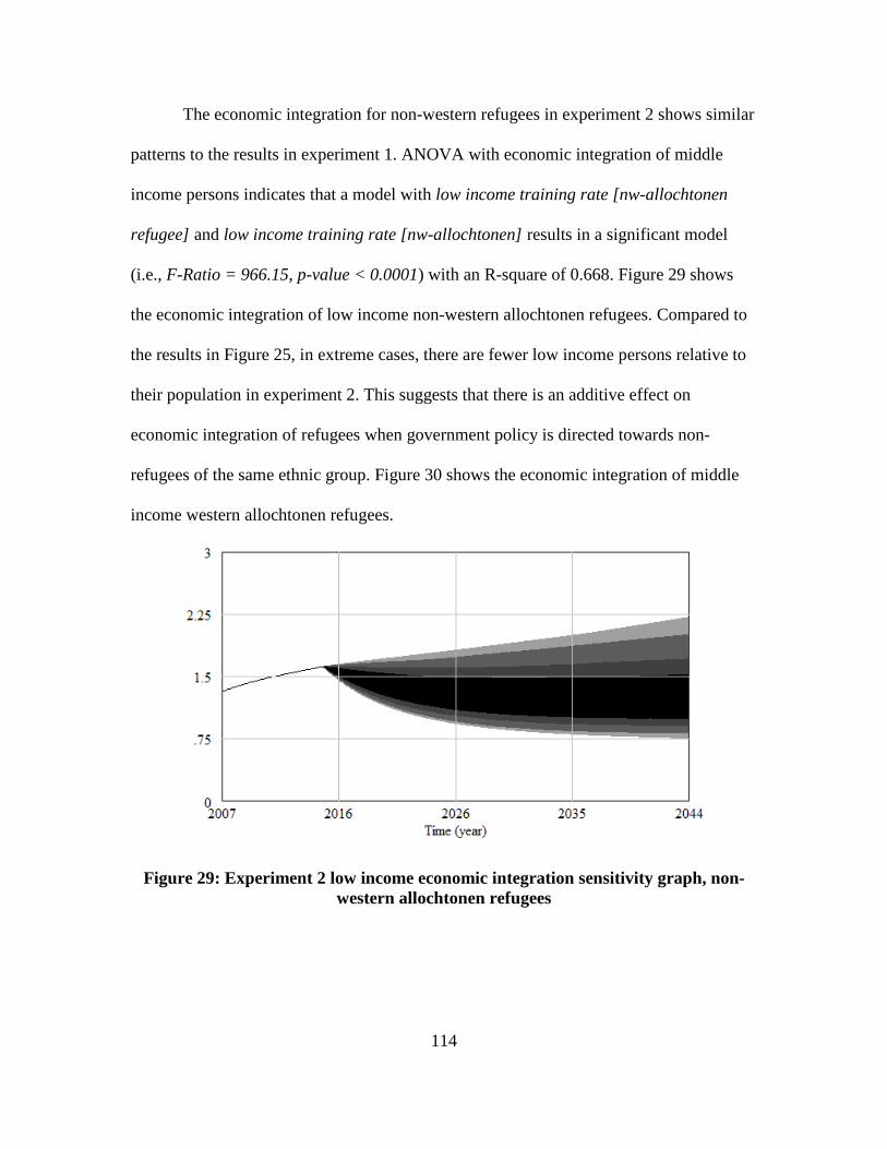
114
The economic integration for non-western refugees in experiment 2 shows similar
patterns to the results in experiment 1. ANOVA with economic integration of middle
income persons indicates that a model with low income training rate [nw-allochtonen
refugee] and low income training rate [nw-allochtonen] results in a significant model
(i.e., F-Ratio = 966.15, p-value < 0.0001) with an R-square of 0.668. Figure 29 shows
the economic integration of low income non-western allochtonen refugees. Compared to
the results in Figure 25, in extreme cases, there are fewer low income persons relative to
their population in experiment 2. This suggests that there is an additive effect on
economic integration of refugees when government policy is directed towards non-
refugees of the same ethnic group. Figure 30 shows the economic integration of middle
income western allochtonen refugees.
Figure 29: Experiment 2 low income economic integration sensitivity graph, non-western allochtonen refugees

115
Figure 30: Experiment 2 middle income economic integration sensitivity graph, non-western allochtonen refugees
Summary
Through experimentation it has been shown that the model indicates that
government programs directed towards refugees can have a positive effect on the
measures of integration for these groups. The results of the experiment also indicate that
there is an additional positive affect on the integration of refugees if policy is
implemented on non-refugee individuals of the same ethnic group. The analytical results
in this analysis and results chapter inform the policy recommendations made in the
following conclusions and recommendations chapter.

116
VI. Conclusions and Recommendations
Overview
The conclusions of this study are framed as answers to the research questions that
were asked at the end of the introduction chapter. The research questions are repeated and
addressed in the following subsection. The responses are a combination of information
from the literature review, model development, and analysis and results chapters.
Conclusions of Research
1. Which factors are the drivers of integration in a city system?
The literature review indicates that economic intervention is an appropriate method to
increase integration of individuals within a city system. This was shown to be the
case within the UDRI model. In addition to economic intervention, language training
seems to have quite a large effect on integration of all types. The impact of language
ability on job market outcomes (as shown in literature) explains this effect.
Additionally, efforts to redistribute persons of lower income (of all ethnic groups)
relieves the pressures of competition for low income jobs within crowded districts
and increases economic outcomes for these individuals.
2. What are the effects of changing assumptions on city system behavior?
The UDRI model is fairly quantitatively sensitive to changes of the assumed
parameters and rates. However, it is not very behaviorally sensitive. This indicates
that the parameters used for this model should be reviewed to assure confidence in the
values. Another method of dealing with uncertainty of parameters is to embrace it by

117
modeling the parameters as probability distributions. Additional available data (at the
appropriate fidelity) should be used to update the parameters within the UDRI model.
3. Which government policies are best suited to address problems with integration?
The model indicates that the government policies that address social, legal and
economic integration are language programs, labor training programs, and low cost
housing construction programs. The UDRI model indicates that these programs in
combination can increase the integration of individuals within a city system. The
policies should focus on both refugee and non-refugee populations of disadvantaged
persons to take advantage of the additive effects of improving outcomes for an entire
ethnic group.
Limitations of Results
The applicability of the results of the UDRI model are limited by the modeling
method, data availability, and the modeling assumptions. The system dynamics model in
this study represents the decisions and movements of individuals throughout the city
system; yet, these are the decisions and movements of the average person. The
parameters calculated from empirical data are representations of the average value for
people within the city. Even if there is data available to determine parameters for groups,
the parameters represent the average person within that group. It should not be forgotten
that in a population of people, there are some who would act similar to the average
person while others would not. System dynamics is not as well-suited for modeling
individual decision making processes as some other methods are (e.g. agent-based
simulation). The UDRI model is a valid representation of a city; nonetheless, the

118
limitations of system dynamics must be understood to appropriately interpret the results
of this study.
It has been mentioned previously throughout this study that if there were more
data available or data available with higher granularity, then the model could be updated
to reflect this information. Not all of the data used within the model development is
representative of the district level in the city of Rotterdam. In each case, the next best,
available replacement has been used to populate the model. This study is conducted with
the understanding that more accurate data would result in a more accurate model;
accordingly, the parameters that were determined using data other than Rotterdam,
district-level, sources were clearly denoted.
Data availability is one of the causal factors of the modeling assumptions made
during model development and validation. In the absence of an appropriate, available
replacement for parameters or structures, the assumption was made that the value or form
remained unchanged from the Sanders model. Changes to decision rules were made
because there was information to support that there existed a difference in the Rotterdam
city system and that it was appropriate and necessary for the purpose of this study to
model that difference. The conclusions made in this study should be viewed through the
lens of the limitations described within this section.
Recommendations for Future Research
Recommendations for future research follow two main paths. The first vein of
future research involves refining the UDRI model. There are plenty of opportunities to
add to this initial formulation of the model. Topics for consideration should include
119
gender-related differences in socio-economic outcomes of refugees, variables that
describe sentiments between groups of people, and the implementation of a transportation
system. The current UDRI formulation does not take into account marital status or sex of
individuals. Research within the field of refugee studies indicates that there are
differences in the social and economic outcomes between male and female asylum
seekers [10], [16], [30]. It would be a worthwhile excursion to add gender dynamics to
the UDRI model.
There are opportunities within the UDRI model to create and implement implied
attitude variables using the information that is already in the system. These variables
could use the differences (or trends in differences) in economic outcomes between groups
of people to quantify feelings. Increased economic disparity between groups would likely
created increased frustration for disadvantaged groups [11]. An increasingly frustrated
person would potentially act according to different decision rules than a person who is
satisfied with their personal circumstances. Adding attitude variables to the UDRI model
would augment the existing social integration measure and add a realistic and relevant
component to refugee integration.
The implementation of a transportation system within the city would allow for the
relaxation of the non-commuting assumption. In this way, the model would be able to
represent the choices people make about whether or not they would like to commute to
their place of employment. This added transportation system should include public
transportation options. Many persons of lower socio-economic status rely on public
transportation systems to commute to and from work. Decisions about transportation

120
options are interrelated with the infrastructure impacts within the city. Adding a
transportation system would capture this dynamic.
The second path of recommended future research is in the field of refugee studies.
This study is focused on refugees, there are other millions of other displaced persons who
are not addressed in the UDRI model. All types of displaced persons are vulnerable; these
people deserve value-added research to help understand their plight and recommend
solutions to the complex issues surrounding displacement. There are other types of
displaced persons who are likely to become more prominent in the future; environmental
refugees are a group of persons that will in all likelihood increase in size as pressures
from drought, rising water levels, and other climate shifts threaten established
communities of people. Researchers from all fields of study can and should contribute to
understanding issues surrounding displaced persons and strive to improve the conditions
for vulnerable people.
Significance of Research
This research offers insights into the dynamics within a city that is affected by
refugee flow. The literature review and modeling in this study further the understanding
of the ways that refugees are affected as they move into cities. Although the UDRI model
has limitations that diminish its realism in some ways, there is still value added for
thinking models that bring understanding to complex social issues. Davis and O’Mahony
of RAND Corporation [67] among others have identified multiple values and benefits
gained from the process of developing data-driven, semi-quantitative models. Models that
describe complex processes are valuable in themselves as thinking models; these models

121
help individuals understand the interactions between components of a system without the
need for a high level of expertise in technical fields (e.g.. mathematics, computer science,
and so forth) [67]. Models such as the UDRI are useful because of the feasibility of
describing and handling social and human components. The UDRI model has plenty of
room for improvements; nonetheless, in its current form, there is value added in the
contribution to understanding of the problems surrounding refugees. The model provides
a foundation for capturing social science insights that can be a guide to data needs for
quantification. The act of modeling provides value in and of itself.
Summary
The UDRI model is a preliminary attempt to bring value and insight to the field of
refugee studies through the use of operations research techniques. This thesis is an early
step in building the body of knowledge in the fields of operations research and refugee
studies. Further research is certainly recommended to expand upon the framework of this
pilot study. Hopefully, this study has increased the awareness of challenges faced by
displaced persons and has inspired a desire for those reading to use their talents and
abilities for the benefit of others.

122
Appendix A: Supplemental Tables
Table 8: District geographic coordinates
District Coordinates
Centrum 51.918159, 4.473938 Delfshaven 51.907092, 4.451218 Overschie 51.938306, 4.431423 Noord 51.931931, 4.459926 Hillegersberg-Schiebroek 51.952033, 4.489160 Kranlingen-Crooswijk 51.918943, 4.522730 Feijenoord 51.895858, 4.502800 Ijsselmonde 51.886354, 4.543441 Pernis 51.888720, 4.389092 Prins Alexander 51.960537, 4.542634 Charlois 51.889008, 4.466833 Hoogvliet 51.861595, 4.358007 Hoek van Holland 51.980651, 4.134087 Rozenburg 51.904419, 4.247127
Table 9: Sensitivity analysis constants and values
Constant Name Low Value Base Value High Value Birth Rate [autochtonen] 0.00218 0.00291 0.00364 Birth Rate [nw-allochtonen] 0.00384 0.00513 0.00641 Birth Rate [w-allochtonen] 0.00308 0.00411 0.00514 Business Opening Normal [A] 0.0035 0.0046 0.0058 Business Opening Normal [B-F] 0.0290 0.0386 0.0483 Business Opening Normal [G+I] 0.0152 0.0202 0.0253 Business Opening Normal [H+J] 0.0404 0.0539 0.0674 Business Opening Normal [K-L] 0.0173 0.0231 0.0289 Business Opening Normal [M-N] 0.0497 0.0662 0.0828 Business Opening Normal [R-U] 0.0443 0.0591 0.0739 Housing Construction Normal [single] 0.002 0.003 0.004 Housing Construction Normal [multi] 0.004 0.006 0.008 Housing Obsolescence Normal 0.0002 0.0003 0.0004 Immigrant Arrival Rate constant[nw-allochtonen] 0.0098 0.013 0.016 Immigrant Arrival Rate constant[w-allochtonen] 0.0029 0.0039 0.0049 Integration Exam Pass Rate constant 0.461 0.615 0.769 NT2 Pass Rate constant 0.461 0.615 0.769

123
Table 10: Experiment factors
Experiment 1 Experiment 2 Range HHCR HI housing construction rate[D1] HHCR HI housing construction rate[D1] [0, 0.01] HHCR HI housing construction rate[D2] HHCR HI housing construction rate[D2] [0, 0.01] HHCR HI housing construction rate[D3] HHCR HI housing construction rate[D3] [0, 0.01] HHCR HI housing construction rate[D4] HHCR HI housing construction rate[D4] [0, 0.01] HHCR HI housing construction rate[D5] HHCR HI housing construction rate[D5] [0, 0.01] HHCR HI housing construction rate[D6] HHCR HI housing construction rate[D6] [0, 0.01] HHCR HI housing construction rate[D7] HHCR HI housing construction rate[D7] [0, 0.01] HHCR HI housing construction rate[D8] HHCR HI housing construction rate[D8] [0, 0.01] HHCR HI housing construction rate[D9] HHCR HI housing construction rate[D9] [0, 0.01] HHCR HI housing construction rate[D10] HHCR HI housing construction rate[D10] [0, 0.01] HHCR HI housing construction rate[D11] HHCR HI housing construction rate[D11] [0, 0.01] HHCR HI housing construction rate[D12] HHCR HI housing construction rate[D12] [0, 0.01] HHCR HI housing construction rate[D13] HHCR HI housing construction rate[D13] [0, 0.01] HHCR HI housing construction rate[D14] HHCR HI housing construction rate[D14] [0, 0.01] Language Program Rate["w-allochtonen refugee"]
Language Program Rate["nw-allochtonen refugee"]
[0, 1.6]
Language Program Rate["nw-allochtonen refugee"]
Language Program Rate["nw-allochtonen "] [0, 1.6]
LHCR LI housing construction rate[D1] LHCR LI housing construction rate[D1] [0, 0.01] LHCR LI housing construction rate[D2] LHCR LI housing construction rate[D2] [0, 0.01] LHCR LI housing construction rate[D3] LHCR LI housing construction rate[D3] [0, 0.01] LHCR LI housing construction rate[D4] LHCR LI housing construction rate[D4] [0, 0.01] LHCR LI housing construction rate[D5] LHCR LI housing construction rate[D5] [0, 0.01] LHCR LI housing construction rate[D6] LHCR LI housing construction rate[D6] [0, 0.01] LHCR LI housing construction rate[D7] LHCR LI housing construction rate[D7] [0, 0.01] LHCR LI housing construction rate[D8] LHCR LI housing construction rate[D8] [0, 0.01] LHCR LI housing construction rate[D9] LHCR LI housing construction rate[D9] [0, 0.01] LHCR LI housing construction rate[D10] LHCR LI housing construction rate[D10] [0, 0.01] LHCR LI housing construction rate[D11] LHCR LI housing construction rate[D11] [0, 0.01]
Refugee Arrival Normal[i, nw-allochtonen refugee] 6.26 8.35 10.44 Refugee Arrival Normal[i, w-allochtonen refugee] 0.3 0.4 0.5 Working Population Arrival Normal [non refugee] 0.028 0.037 0.046 Working Population Departures Normal[non refugee] 0.035 0.047 0.059 Working Population internal out-of-zone movement normal 0.021 0.028 0.035

124
LHCR LI housing construction rate[D12] LHCR LI housing construction rate[D12] [0, 0.01] LHCR LI housing construction rate[D13] LHCR LI housing construction rate[D13] [0, 0.01] LHCR LI housing construction rate[D14] LHCR LI housing construction rate[D14] [0, 0.01] LTR LI training rate["w-allochtonen refugee"]
LTR LI training rate["nw-allochtonen refugee"]
[0, 0.1]
LTR LI training rate["nw-allochtonen refugee"]
LTR LI training rate["nw-allochtonen"] [0, 0.1]
MHCR MI housing construction rate[D1] MHCR MI housing construction rate[D1] [0, 0.01] MHCR MI housing construction rate[D2] MHCR MI housing construction rate[D2] [0, 0.01] MHCR MI housing construction rate[D3] MHCR MI housing construction rate[D3] [0, 0.01] MHCR MI housing construction rate[D4] MHCR MI housing construction rate[D4] [0, 0.01] MHCR MI housing construction rate[D5] MHCR MI housing construction rate[D5] [0, 0.01] MHCR MI housing construction rate[D6] MHCR MI housing construction rate[D6] [0, 0.01] MHCR MI housing construction rate[D7] MHCR MI housing construction rate[D7] [0, 0.01] MHCR MI housing construction rate[D8] MHCR MI housing construction rate[D8] [0, 0.01] MHCR MI housing construction rate[D9] MHCR MI housing construction rate[D9] [0, 0.01] MHCR MI housing construction rate[D10] MHCR MI housing construction rate[D10] [0, 0.01] MHCR MI housing construction rate[D11] MHCR MI housing construction rate[D11] [0, 0.01] MHCR MI housing construction rate[D12] MHCR MI housing construction rate[D12] [0, 0.01] MHCR MI housing construction rate[D13] MHCR MI housing construction rate[D13] [0, 0.01] MHCR MI housing construction rate[D14] MHCR MI housing construction rate[D14] [0, 0.01] MTR MI training rate["w-allochtonen refugee"]
MTR MI training rate["nw-allochtonen refugee"]
[0, 0.1]
MTR MI training rate["nw-allochtonen refugee"]
MTR MI training rate["nw-allochtonen"] [0, 0.1]
Table 11: Experiment responses
Experiment 1 Experiment 2
Social Integration [w allochtonen refugee] Social Integration [nw allochtonen] Social Integration [nw allochtonen refugee] Social Integration [nw allochtonen refugee] Economic Integration LI [w allochtonen refugee] Economic Integration LI [nw allochtonen] Economic Integration LI [nw allochtonen refugee] Economic Integration LI [nw allochtonen refugee] Economic Integration MI [w allochtonen refugee] Economic Integration MI [nw allochtonen] Economic Integration MI [nw allochtonen refugee] Economic Integration MI [nw allochtonen refugee] Economic Integration HI [w allochtonen refugee] Economic Integration HI [nw allochtonen] Economic Integration HI [nw allochtonen refugee] Economic Integration HI [nw allochtonen refugee] Legal Integration Total [w allochtonen refugee] Legal Integration Total [nw allochtonen] Legal Integration Total [nw allochtonen refugee] Legal Integration Total [nw allochtonen refugee]

125
Appendix B: Vensim Model Code
******************************************************** .Control ********************************************************~ Simulation Control Parameters | class : A,"B-F","G+I","H+J","K-L","M-N","R-U" ~ ~ | FINAL TIME = 2044 ~ year ~ The final time for the simulation. | group : non refugee,refugee ~ ~ | i : D1,D2,D3,D4,D5,D6,D7,D8,D9,D10,D11,D12,D13,D14 ~ ~ | INITIAL TIME = 2007 ~ year ~ The initial time for the simulation. | k : D1,D2,D3,D4,D5,D6,D7,D8,D9,D10,D11,D12,D13,D14 ~ ~ | non refugee : autochtonen,"w-allochtonen","nw-allochtonen" ~ ~ | "nw-allochtonen total" : "nw-allochtonen","nw-allochtonen refugee" ~ ~ | refugee : "w-allochtonen refugee","nw-allochtonen refugee" ~ ~ | SAVEPER = 1 / 12 ~ year [0,?] ~ The frequency with which output is stored. | TIME STEP = 1 / 12 ~ year [0,?] ~ The time step for the simulation. | type : single,multi ~ ~ | "w-allochtonen total" : "w-allochtonen","w-allochtonen refugee" ~ ~ | ******************************************************** .Education ********************************************************~ | Adult Education Initial[i] = 0.12, 0.08, 0.03, 0.08, 0.04, 0.12, 0.04, 0.03, 0.02, 0.04\ , 0.04, 0.02, 0.03, 0.02 ~ ~ | "Arrive 14+"[i,group] = Youth Arrivals[i,group] * ( 4 / 14) ~ ~ | Arrive HAVO 1[i,group] = "Youth 14+ Arrivals"[i,group] * ( "VO2-HAVO1 Rate constant"[\ i,group] / "P8-VO1 rate constant"[group] ) * ( 1 / 4) ~~ 28.5/94 for HAVO ratio. 1/3 to divide by 4 years | Arrive HAVO 2[i,group] = "Youth 14+ Arrivals"[i,group] * ( "VO2-HAVO1 Rate constant"[\

126
i,group] / "P8-VO1 rate constant"[group] ) * ( 1 / 4) ~ ~ | Arrive HAVO 3[i,group] = "Youth 14+ Arrivals"[i,group] * ( "VO2-HAVO1 Rate constant"[\ i,group] / "P8-VO1 rate constant"[group] ) * ( 1 / 4) ~ ~ | Arrive Primary 1[i,group] = Youth Arrivals[i,group] * ( 1 / 14) ~~ 1/14 to equally divide into all 14 years of mandatory education | Arrive Primary 2[i,group] = Youth Arrivals[i,group] * ( 1 / 14) ~~ 1/14 to equally divide into all 14 years of mandatory education | Arrive Primary 3[i,group] = Youth Arrivals[i,group] * ( 1 / 14) ~~ 1/14 to equally divide into all 14 years of mandatory education | Arrive Primary 4[i,group] = Youth Arrivals[i,group] * ( 1 / 14) ~~ 1/14 to equally divide into all 14 years of mandatory education | Arrive Primary 5[i,group] = Youth Arrivals[i,group] * ( 1 / 14) ~~ 1/14 to equally divide into all 14 years of mandatory education | Arrive Primary 6[i,group] = Youth Arrivals[i,group] * ( 1 / 14) ~~ 1/14 to equally divide into all 14 years of mandatory education | Arrive Primary 7[i,group] = Youth Arrivals[i,group] * ( 1 / 14) ~~ 1/14 to equally divide into all 14 years of mandatory education | Arrive Primary 8[i,group] = Youth Arrivals[i,group] * ( 1 / 14) ~~ 1/14 to equally divide into all 14 years of mandatory education | "Arrive PRO/VSO"[i,group] = Youth Arrivals[i,group] * ( 2 / 14) * "P8-PRO/VSO1 Rate constant"\ [group] ~ ~ | Arrive VMBO 1[i,group] = "Youth 14+ Arrivals"[i,group] * ( "VO2-VMBO1 Rate constant"[\ i,group] / "P8-VO1 rate constant"[group] ) * ( 1 / 4) ~~ 49/94 for VMBO ratio. 1/4 to divide by years | Arrive VMBO 2[i,group] = "Youth 14+ Arrivals"[i,group] * ( "VO2-VMBO1 Rate constant"[\ i,group] / "P8-VO1 rate constant"[group] ) * ( 1 / 4) ~ ~ | Arrive VO 1[i,group] = Youth Arrivals[i,group] * ( 1 / 14) * "P8-VO1 rate constant"[group\ ] ~ Person/year ~ | Arrive VO 2[i,group] = Youth Arrivals[i,group] * ( 1 / 14) * "P8-VO1 rate constant"[group\ ] ~ Person/year ~ | Arrive VWO 1[i,group] = "Youth 14+ Arrivals"[i,group] * ( "VO2-VWO1 Rate constant"[i,\ group] / "P8-VO1 rate constant"[group] ) * ( 1 / 4) ~~ 15.5/94 is the VWO ratio. 1/4 divides it by 4 years | Arrive VWO 2[i,group] = "Youth 14+ Arrivals"[i,group] * ( "VO2-VWO1 Rate constant"[i,\ group] / "P8-VO1 rate constant"[group] ) * ( 1 / 4) ~

127
~ | Arrive VWO 3[i,group] = "Youth 14+ Arrivals"[i,group] * ( "VO2-VWO1 Rate constant"[i,\ group] / "P8-VO1 rate constant"[group] ) * ( 1 / 4) ~ ~ | Arrive VWO 4[i,group] = "Youth 14+ Arrivals"[i,group] * ( "VO2-VWO1 Rate constant"[i,\ group] / "P8-VO1 rate constant"[group] ) * ( 1 / 4) ~ ~ | Births to Education[i,group] = Birthed Children[i,group] / 4 * PULSE TRAIN ( 0, 1 / 12\ , 1, FINAL TIME ) ~ Person/year ~ /4 for four years until school begins | Education HI Class Ratio[class] = 0.00562, 0.21744, 0.23993, 0.13381, 0.07138, 0.24113\ , 0.09069 ~ ~ | Education LI Class Ratio[autochtonen,class] = 0.00562, 0.21744, 0.23993, 0.13381, 0.07138\ , 0.24113, 0.09069 ~~| Education LI Class Ratio["nw-allochtonen",class] = 0.001873, 0.1461, 0.240855, 0.13473\ , 0.14276, 0.24205, 0.09161 ~~| Education LI Class Ratio["w-allochtonen",class] = 0.00562, 0.21744, 0.23993, 0.13381,\ 0.07138, 0.24113, 0.09069 ~~| Education LI Class Ratio["nw-allochtonen refugee",class] = 0.001873, 0.1461, 0.240855\ , 0.13473, 0.14276, 0.24205, 0.09161 ~~| Education LI Class Ratio["w-allochtonen refugee",class] = 0.00562, 0.21744, 0.23993, \ 0.13381, 0.07138, 0.24113, 0.09069 ~ ~ | Education MI Class Ratio[class] = 0.00562, 0.21744, 0.23993, 0.13381, 0.07138, 0.24113\ , 0.09069 ~ ~ | Education Population[i,group] = Primary Education[i,group] + VO[i,group] + "PRO/VSO"[\ i,group] + VMBO[i,group] + VWO[i,group] + HAVO[i,group] + "MBO-1"[i,group] + "MBO-2"\ [i,group] + "MBO-3"[i,group] + "MBO-4"[i,group] + HBO[i,group] + WO[i,group] + "PRO/VSO Graduates"\ [i,group] + VO Dropouts[i,group] + VMBO Graduates[i,group] + "VWO/HAVO Dropouts"[i,\ group] + "MBO-2 Dropouts"[i,group] + "MBO-3/4 Dropouts"[i,group] + "WO/HBO Dropouts"\ [i,group] ~ ~ | Education to HI[i,group] = INTEG( HBO to HI[i,group] + "MBO-4 to HI"[i,group] + WO to HI\ [i,group] - SUM ( Education to HI Rate[i,group,class!] ) , WO to HI[i,group] + HBO to HI\ [i,group] + "MBO-4 to HI"[i,group] ) ~ ~ | Education to HI Rate[i,group,class] = Education to HI[i,group] * Education HI Class Ratio\ [class] * PULSE TRAIN ( 0, 1 / 12, 1, FINAL TIME ) ~ Person/year ~ | Education to LI[i,group] = INTEG( "MBO-1 to LI"[i,group] + "MBO-2 to LI"[i,group] + "PRO/VSO Graduate to LI"\ [i,group] + VMBO Graduate to LI[i,group] + VO to LI[i,group] + "VWO/HAVO to LI"[i,group\ ] + "Youth 14+ to LI"[i,group] - SUM ( Education to LI Rate[i,group,class!] ) , 0) ~ Person ~ | Education to LI Rate[i,group,class] = Education to LI[i,group] * Education LI Class Ratio\ [group,class] * PULSE TRAIN ( 0, 1 / 12, 1, FINAL TIME ) ~ Person/year ~ | Education to MI[i,group] = INTEG( "MBO-2 to MI"[i,group] + "MBO-3 to MI"[i,group] + "MBO-3/4 to MI"\ [i,group] + "WO/HBO to MI"[i,group] - SUM ( Education to MI Rate[i,group,class!] ) \ , "MBO-2 to MI"[i,group] + "MBO-3 to MI"[i,group] + "MBO-3/4 to MI"[i,group] + "WO/HBO to MI"\ [i,group] ) ~ Person ~ | Education to MI Rate[i,group,class] = Education to MI[i,group] * Education MI Class Ratio\ [class] * PULSE TRAIN ( 0, 1 / 12, 1, FINAL TIME )

128
~ Person/year ~ | HAVO[i,group] = HAVO 1[i,group] + HAVO 2[i,group] + HAVO 3[i,group] ~ ~ | HAVO 1[i,group] = INTEG( Arrive HAVO 1[i,group] + "VO2-HAVO1"[i,group] - "HAVO1-HAVO2"\ [i,group] + IF THEN ELSE ( HAVO 1[i,group] + ( HAVO 1[i,group] * Working Population Net Zone Movement\ [i,group] * Youth Arrival Rate constant[group] / Mandatory Education Population[i,group\ ] ) <= 0, 0, ( HAVO 1[i,group] * Working Population Net Zone Movement[i,group] * Youth Arrival Rate constant\ [group] / Mandatory Education Population[i,group] ) ) , VO 2[i,group] * "VO2-HAVO1 Rate constant"\ [i,group] ) ~ Person ~ | HAVO 2[i,group] = INTEG( Arrive HAVO 2[i,group] + "HAVO1-HAVO2"[i,group] - "HAVO2-HAVO3"\ [i,group] + IF THEN ELSE ( HAVO 2[i,group] + ( Working Population Net Zone Movement\ [i,group] * Youth Arrival Rate constant[group] * HAVO 2[i,group] / Mandatory Education Population\ [i,group] ) <= 0, 0, ( Working Population Net Zone Movement[i,group] * Youth Arrival Rate constant\ [group] * HAVO 2[i,group] / Mandatory Education Population[i,group] ) ) , HAVO 1[i,\ group] ) ~ Person ~ | HAVO 3[i,group] = INTEG( Arrive HAVO 3[i,group] + "HAVO2-HAVO3"[i,group] + "VMBO2-HAVO3"\ [i,group] - HAVO Dropout Rate[i,group] - "HAVO3-HBO1"[i,group] - "HAVO3-MBO-41"[i,group\ ] + IF THEN ELSE ( HAVO 3[i,group] + ( Working Population Net Zone Movement[i,group\ ] * Youth Arrival Rate constant[group] * HAVO 3[i,group] / Mandatory Education Population\ [i,group] ) <= 0, 0, ( Working Population Net Zone Movement[i,group] * Youth Arrival Rate constant\ [group] * HAVO 3[i,group] / Mandatory Education Population[i,group] ) ) , HAVO 2[i,\ group] + VMBO 2[i,group] * "VMBO2-HAVO3 Rate constant"[i,group] ) ~ Person ~ | HAVO Dropout Rate[i,group] = HAVO 3[i,group] * ( HAVO Dropout Rate constant[i,group] \ / HAVO3 Exit Rate constant[i,group] ) * PULSE TRAIN ( 0, 1 / 12, 1, FINAL TIME ) ~ Person/year ~ | HAVO Dropout Rate constant[i,group] = 0.005 * Economic Integration HI district[i,group\ ] ~ ~ | "HAVO1-HAVO2"[i,group] = HAVO 1[i,group] * PULSE TRAIN ( 0, 1 / 12, 1, FINAL TIME ) ~ Person/year ~ | "HAVO2-HAVO3"[i,group] = HAVO 2[i,group] * PULSE TRAIN ( 0, 1 / 12, 1, FINAL TIME ) ~ Person/year ~ | HAVO3 Exit Rate constant[i,group] = "VO2-HAVO1 Rate constant"[i,group] + "VMBO2-HAVO3 Rate constant"\ [i,group] ~ ~ | "HAVO3-HBO1 Rate constant"[i,group] = 0.27 ~ ~ | "HAVO3-HBO1"[i,group] = HAVO 3[i,group] * ( "HAVO3-HBO1 Rate constant"[i,group] / HAVO3 Exit Rate constant\ [i,group] ) * PULSE TRAIN ( 0, 1 / 12, 1, FINAL TIME ) ~ Person/year ~ | "HAVO3-MBO-41 Rate constant"[group] = 0.04 ~ ~ | "HAVO3-MBO-41"[i,group] = HAVO 3[i,group] * ( "HAVO3-MBO-41 Rate constant"[group] / HAVO3 Exit Rate constant\ [i,group] ) * PULSE TRAIN ( 0, 1 / 12, 1, FINAL TIME ) ~ Person/year ~ | HBO[i,group] = HBO 1[i,group] + HBO 2[i,group] + HBO 3[i,group] + HBO 4[i,group] ~ ~ | HBO 1[i,group] = INTEG( "HAVO3-HBO1"[i,group] + "MBO-44-HBO1"[i,group] - "HBO1-HBO2"[\ i,group] - "HBO1-WO1"[i,group] , HAVO 3[i,group] * "HAVO3-HBO1 Rate constant"[i,group\ ] + "MBO-4 4"[i,group] * "MBO-44-HBO1 Rate constant"[i,group] + Higher Education Population Initial\

129
[i,group] * ( "HAVO3-HBO1 Rate constant"[i,group] / ( 90 * 4) ) ) ~ Person ~ | HBO 1 Exit Rate constant[i,group] = "HAVO3-HBO1 Rate constant"[i,group] + "MBO-44-HBO1 Rate constant"\ [i,group] ~ ~ | HBO 2[i,group] = INTEG( "HBO1-HBO2"[i,group] - "HBO2-HBO3"[i,group] , HBO 1[i,group] \ ) ~ Person ~ | HBO 3[i,group] = INTEG( "HBO2-HBO3"[i,group] - "HBO3-HBO4"[i,group] , HBO 2[i,group] \ ) ~ Person ~ | HBO 4[i,group] = INTEG( "HBO3-HBO4"[i,group] - HBO Dropout Rate[i,group] - HBO to HI[\ i,group] , HBO 3[i,group] ) ~ Person ~ | HBO Dropout Rate[i,group] = HBO 4[i,group] * ( HBO Dropout Rate constant[group] / "HBO1-HBO2 Rate constant"\ [i,group] ) * PULSE TRAIN ( 0, 1 / 12, 1, FINAL TIME ) ~ Person/year ~ | HBO Dropout Rate constant[group] = 0.16 ~ ~ | HBO to HI[i,group] = HBO 4[i,group] * ( HBO to HI Rate constant[group] / "HBO1-HBO2 Rate constant"\ [i,group] ) * PULSE TRAIN ( 0, 1 / 12, 1, FINAL TIME ) ~ Person/year ~ | HBO to HI Rate constant[group] = 0.25 ~ ~ | "HBO1-HBO2 Rate constant"[i,group] = HBO 1 Exit Rate constant[i,group] - "HBO1-WO1 Rate constant"\ [i,group] ~ ~ | "HBO1-HBO2"[i,group] = HBO 1[i,group] * ( "HBO1-HBO2 Rate constant"[i,group] / HBO 1 Exit Rate constant\ [i,group] ) * PULSE TRAIN ( 0, 1 / 12, 1, FINAL TIME ) ~ ~ | "HBO1-WO1 Rate constant"[i,group] = 0.01 ~ ~ | "HBO1-WO1"[i,group] = HBO 1[i,group] * ( "HBO1-WO1 Rate constant"[i,group] / HBO 1 Exit Rate constant\ [i,group] ) * PULSE TRAIN ( 0, 1 / 12, 1, FINAL TIME ) ~ Person/year ~ | "HBO2-HBO3"[i,group] = HBO 2[i,group] * PULSE TRAIN ( 0, 1 / 12, 1, FINAL TIME ) ~ ~ | "HBO3-HBO4"[i,group] = HBO 3[i,group] * PULSE TRAIN ( 0, 1 / 12, 1, FINAL TIME ) ~ ~ | Higher Education Population Initial[i,group] = SUM ( Working Population[i,group,class\ !] ) * Adult Education Initial[i] ~ ~ | Mandatory Education Population[i,group] = Primary Education[i,group] + "PRO/VSO"[i,group\ ] + VO[i,group] + VWO[i,group] + HAVO[i,group] + VMBO[i,group] + VO Dropouts[i,group\ ] + "PRO/VSO Graduates"[i,group] + "Youth 14+ Arrivals Not in Education"[i,group] +\ VMBO Graduates[i,group] ~ ~ | "MBO-1 1"[i,group] = INTEG( "VMBO2-MBO-11"[i,group] - "MBO-1 to LI"[i,group] , VMBO 2\ [i,group] * "VMBO2-MBO-11 Rate constant"[group] + Higher Education Population Initial\ [i,group] * ( "VMBO2-MBO-11 Rate constant"[group] / ( 90) ) ) ~ Person

130
~ | "MBO-1 to LI"[i,group] = "MBO-1 1"[i,group] * PULSE TRAIN ( 0, 1 / 12, 1, FINAL TIME \ ) ~ Person/year ~ | "MBO-1"[i,group] = "MBO-1 1"[i,group] ~ ~ | "MBO-2 1"[i,group] = INTEG( "VMBO2-MBO-21"[i,group] - "MBO-21-MBO-22"[i,group] , VMBO 2\ [i,group] * "VMBO2-MBO-21 Rate constant"[group] + Higher Education Population Initial\ [i,group] * ( "VMBO2-MBO-21 Rate constant"[group] / ( 90 * 3) ) ) ~ Person ~ | "MBO-2 2"[i,group] = INTEG( "MBO-21-MBO-22"[i,group] - "MBO-22-MBO-23"[i,group] , "MBO-2 1"\ [i,group] ) ~ Person ~ | "MBO-2 3"[i,group] = INTEG( "MBO-22-MBO-23"[i,group] - "MBO-2 Dropout Rate"[i,group] \ - "MBO-2 to MI"[i,group] , "MBO-2 2"[i,group] ) ~ Person ~ | "MBO-2 Dropout Rate constant"[group] = 0.03 ~ ~ | "MBO-2 Dropout Rate"[i,group] = "MBO-2 3"[i,group] * ( "MBO-2 Dropout Rate constant"[\ group] / "VMBO2-MBO-21 Rate constant"[group] ) * PULSE TRAIN ( 0, 1 / 12, 1, FINAL TIME\ ) ~ Person/year ~ | "MBO-2 Dropouts"[i,group] = INTEG( "MBO-2 Dropout Rate"[i,group] - "MBO-2 to LI"[i,group\ ] , "MBO-2 Dropout Rate"[i,group] ) ~ ~ | "MBO-2 to LI"[i,group] = "MBO-2 Dropouts"[i,group] * PULSE TRAIN ( 0, 1 / 12, 1, FINAL TIME\ ) ~ Person/year ~ | "MBO-2 to MI Rate constant"[group] = 0.06 ~ ~ | "MBO-2 to MI"[i,group] = "MBO-2 3"[i,group] * ( "MBO-2 to MI Rate constant"[group] / \ "VMBO2-MBO-21 Rate constant"[group] ) * PULSE TRAIN ( 0, 1 / 12, 1, FINAL TIME ) ~ Person/year ~ | "MBO-2"[i,group] = "MBO-2 1"[i,group] + "MBO-2 2"[i,group] + "MBO-2 3"[i,group] ~ ~ | "MBO-21-MBO-22"[i,group] = "MBO-2 1"[i,group] * PULSE TRAIN ( 0, 1 / 12, 1, FINAL TIME\ ) ~ Person/year ~ | "MBO-22-MBO-23"[i,group] = "MBO-2 2"[i,group] * PULSE TRAIN ( 0, 1 / 12, 1, FINAL TIME\ ) ~ Person/year ~ | "MBO-3 1"[i,group] = INTEG( "VMBO2-MBO-31"[i,group] - "MBO-31-MBO-32"[i,group] , VMBO 2\ [i,group] * "VMBO2-MBO-31 Rate constant"[group] + Higher Education Population Initial\ [i,group] * ( "VMBO2-MBO-31 Rate constant"[group] / ( 90 * 4) ) ) ~ Person ~ | "MBO-3 2"[i,group] = INTEG( "MBO-31-MBO-32"[i,group] - "MBO-32-MBO-33"[i,group] , "MBO-3 1"\ [i,group] ) ~ Person ~ | "MBO-3 3"[i,group] = INTEG( "MBO-32-MBO-33"[i,group] - "MBO-33-MBO-34"[i,group] , "MBO-3 2"\ [i,group] ) ~ Person ~ |

131
"MBO-3 4"[i,group] = INTEG( "MBO-33-MBO-34"[i,group] - "MBO-3 Dropout Rate"[i,group] \ - "MBO-3 to MI"[i,group] , "MBO-3 3"[i,group] ) ~ Person ~ | "MBO-3 Dropout Rate constant"[group] = 0.02 ~ ~ | "MBO-3 Dropout Rate"[i,group] = "MBO-3 4"[i,group] * ( "MBO-3 Dropout Rate constant"[\ group] / "VMBO2-MBO-31 Rate constant"[group] ) * PULSE TRAIN ( 0, 1 / 12, 1, FINAL TIME\ ) ~ Person/year ~ | "MBO-3 to MI Rate constant"[group] = 0.04 ~ ~ | "MBO-3 to MI"[i,group] = "MBO-3 4"[i,group] * ( "MBO-3 to MI Rate constant"[group] / \ "VMBO2-MBO-31 Rate constant"[group] ) * PULSE TRAIN ( 0, 1 / 12, 1, FINAL TIME ) ~ Person/year ~ | "MBO-3"[i,group] = "MBO-3 1"[i,group] + "MBO-3 2"[i,group] + "MBO-3 3"[i,group] + "MBO-3 4"\ [i,group] ~ ~ | "MBO-3/4 Dropouts"[i,group] = INTEG( "MBO-3 Dropout Rate"[i,group] + "MBO-4 Dropout Rate"\ [i,group] - "MBO-3/4 to MI"[i,group] , "MBO-4 Dropout Rate"[i,group] + "MBO-3 Dropout Rate"\ [i,group] ) ~ ~ | "MBO-3/4 to MI"[i,group] = "MBO-3/4 Dropouts"[i,group] * PULSE TRAIN ( 0, 1 / 12, 1, \ FINAL TIME ) ~ Person/year ~ | "MBO-31-MBO-32"[i,group] = "MBO-3 1"[i,group] * PULSE TRAIN ( 0, 1 / 12, 1, FINAL TIME\ ) ~ Person/year ~ | "MBO-32-MBO-33"[i,group] = "MBO-3 2"[i,group] * PULSE TRAIN ( 0, 1 / 12, 1, FINAL TIME\ ) ~ Person/year ~ | "MBO-33-MBO-34"[i,group] = "MBO-3 3"[i,group] * PULSE TRAIN ( 0, 1 / 12, 1, FINAL TIME\ ) ~ Person/year ~ | "MBO-4 1"[i,group] = INTEG( "HAVO3-MBO-41"[i,group] + "VMBO2-MBO-41"[i,group] - "MBO-41-MBO-42"\ [i,group] , VMBO 2[i,group] * "VMBO2-MBO-41 Rate constant"[group] + HAVO 3[i,group]\ * "HAVO3-MBO-41 Rate constant"[group] + Higher Education Population Initial[i,group\ ] * ( ( "VMBO2-MBO-41 Rate constant"[group] + "HAVO3-MBO-41 Rate constant"[group] )\ / ( 90 * 4) ) ) ~ Person ~ | "MBO-4 2"[i,group] = INTEG( "MBO-41-MBO-42"[i,group] - "MBO-42-MBO-43"[i,group] , "MBO-4 1"\ [i,group] ) ~ Person ~ | "MBO-4 3"[i,group] = INTEG( "MBO-42-MBO-43"[i,group] - "MBO-43-MBO-44"[i,group] , "MBO-4 2"\ [i,group] ) ~ Person ~ | "MBO-4 4 Exit Rate constant"[group] = "HAVO3-MBO-41 Rate constant"[group] + "VMBO2-MBO-41 Rate constant"\ [group] ~ ~ | "MBO-4 4"[i,group] = INTEG( "MBO-43-MBO-44"[i,group] - "MBO-4 Dropout Rate"[i,group] \ - "MBO-4 to HI"[i,group] - "MBO-44-HBO1"[i,group] , "MBO-4 3"[i,group] ) ~ Person ~ | "MBO-4 Dropout Rate constant"[group] = 0.05
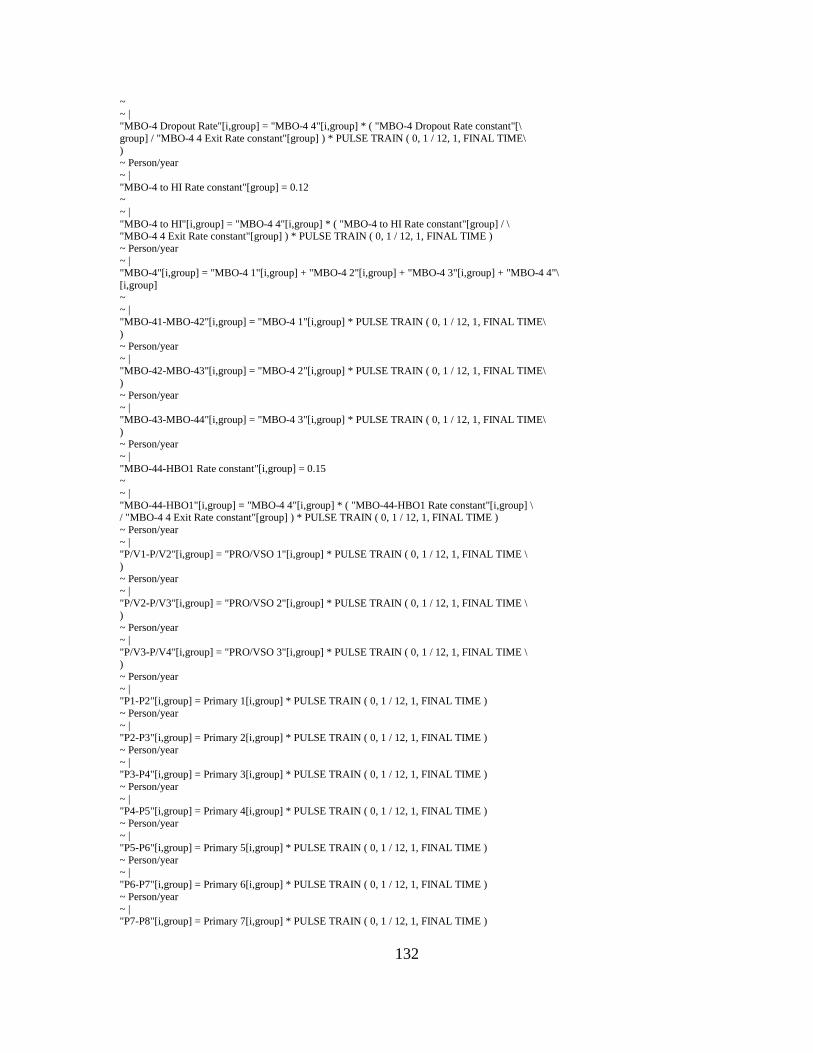
132
~ ~ | "MBO-4 Dropout Rate"[i,group] = "MBO-4 4"[i,group] * ( "MBO-4 Dropout Rate constant"[\ group] / "MBO-4 4 Exit Rate constant"[group] ) * PULSE TRAIN ( 0, 1 / 12, 1, FINAL TIME\ ) ~ Person/year ~ | "MBO-4 to HI Rate constant"[group] = 0.12 ~ ~ | "MBO-4 to HI"[i,group] = "MBO-4 4"[i,group] * ( "MBO-4 to HI Rate constant"[group] / \ "MBO-4 4 Exit Rate constant"[group] ) * PULSE TRAIN ( 0, 1 / 12, 1, FINAL TIME ) ~ Person/year ~ | "MBO-4"[i,group] = "MBO-4 1"[i,group] + "MBO-4 2"[i,group] + "MBO-4 3"[i,group] + "MBO-4 4"\ [i,group] ~ ~ | "MBO-41-MBO-42"[i,group] = "MBO-4 1"[i,group] * PULSE TRAIN ( 0, 1 / 12, 1, FINAL TIME\ ) ~ Person/year ~ | "MBO-42-MBO-43"[i,group] = "MBO-4 2"[i,group] * PULSE TRAIN ( 0, 1 / 12, 1, FINAL TIME\ ) ~ Person/year ~ | "MBO-43-MBO-44"[i,group] = "MBO-4 3"[i,group] * PULSE TRAIN ( 0, 1 / 12, 1, FINAL TIME\ ) ~ Person/year ~ | "MBO-44-HBO1 Rate constant"[i,group] = 0.15 ~ ~ | "MBO-44-HBO1"[i,group] = "MBO-4 4"[i,group] * ( "MBO-44-HBO1 Rate constant"[i,group] \ / "MBO-4 4 Exit Rate constant"[group] ) * PULSE TRAIN ( 0, 1 / 12, 1, FINAL TIME ) ~ Person/year ~ | "P/V1-P/V2"[i,group] = "PRO/VSO 1"[i,group] * PULSE TRAIN ( 0, 1 / 12, 1, FINAL TIME \ ) ~ Person/year ~ | "P/V2-P/V3"[i,group] = "PRO/VSO 2"[i,group] * PULSE TRAIN ( 0, 1 / 12, 1, FINAL TIME \ ) ~ Person/year ~ | "P/V3-P/V4"[i,group] = "PRO/VSO 3"[i,group] * PULSE TRAIN ( 0, 1 / 12, 1, FINAL TIME \ ) ~ Person/year ~ | "P1-P2"[i,group] = Primary 1[i,group] * PULSE TRAIN ( 0, 1 / 12, 1, FINAL TIME ) ~ Person/year ~ | "P2-P3"[i,group] = Primary 2[i,group] * PULSE TRAIN ( 0, 1 / 12, 1, FINAL TIME ) ~ Person/year ~ | "P3-P4"[i,group] = Primary 3[i,group] * PULSE TRAIN ( 0, 1 / 12, 1, FINAL TIME ) ~ Person/year ~ | "P4-P5"[i,group] = Primary 4[i,group] * PULSE TRAIN ( 0, 1 / 12, 1, FINAL TIME ) ~ Person/year ~ | "P5-P6"[i,group] = Primary 5[i,group] * PULSE TRAIN ( 0, 1 / 12, 1, FINAL TIME ) ~ Person/year ~ | "P6-P7"[i,group] = Primary 6[i,group] * PULSE TRAIN ( 0, 1 / 12, 1, FINAL TIME ) ~ Person/year ~ | "P7-P8"[i,group] = Primary 7[i,group] * PULSE TRAIN ( 0, 1 / 12, 1, FINAL TIME )

133
~ Person/year ~ | "P8-PRO/VSO1 Rate constant"[group] = 0.06 ~ Fraction/year ~ | "P8-PRO/VSO1"[i,group] = Primary 8[i,group] * "P8-PRO/VSO1 Rate constant"[group] * PULSE TRAIN\ ( 0, 1 / 12, 1, FINAL TIME ) ~ Person/year ~ | "P8-VO1 rate constant"[group] = 0.94 ~ ~ | "P8-VO1"[i,group] = Primary 8[i,group] * "P8-VO1 rate constant"[group] * PULSE TRAIN \ ( 0, 1 / 12, 1, FINAL TIME ) ~ Person/year ~ | Primary 1[i,group] = INTEG( Arrive Primary 1[i,group] + Births to Education[i,group] \ - "P1-P2"[i,group] + IF THEN ELSE ( Primary 1[i,group] + ( Working Population Net Zone Movement\ [i,group] * Youth Arrival Rate constant[group] * Primary 1[i,group] / Mandatory Education Population\ [i,group] ) <= 0, 0, ( Working Population Net Zone Movement[i,group] * Youth Arrival Rate constant\ [group] * Primary 1[i,group] / Mandatory Education Population[i,group] ) ) , Youth Education Initial\ [i,group] ) ~ Person ~ | Primary 2[i,group] = INTEG( Arrive Primary 2[i,group] + "P1-P2"[i,group] - "P2-P3"[i,\ group] + IF THEN ELSE ( Primary 2[i,group] + ( Working Population Net Zone Movement\ [i,group] * Youth Arrival Rate constant[group] * Primary 2[i,group] / Mandatory Education Population\ [i,group] ) <= 0, 0, ( Working Population Net Zone Movement[i,group] * Youth Arrival Rate constant\ [group] * Primary 2[i,group] / Mandatory Education Population[i,group] ) ) , Youth Education Initial\ [i,group] ) ~ Person ~ | Primary 3[i,group] = INTEG( Arrive Primary 3[i,group] + "P2-P3"[i,group] - "P3-P4"[i,\ group] + IF THEN ELSE ( Primary 3[i,group] + ( Working Population Net Zone Movement\ [i,group] * Youth Arrival Rate constant[group] * Primary 3[i,group] / Mandatory Education Population\ [i,group] ) <= 0, 0, ( Working Population Net Zone Movement[i,group] * Youth Arrival Rate constant\ [group] * Primary 3[i,group] / Mandatory Education Population[i,group] ) ) , Youth Education Initial\ [i,group] ) ~ Person ~ | Primary 4[i,group] = INTEG( Arrive Primary 4[i,group] + "P3-P4"[i,group] - "P4-P5"[i,\ group] + IF THEN ELSE ( Primary 4[i,group] + ( Working Population Net Zone Movement\ [i,group] * Youth Arrival Rate constant[group] * Primary 4[i,group] / Mandatory Education Population\ [i,group] ) <= 0, 0, ( Working Population Net Zone Movement[i,group] * Youth Arrival Rate constant\ [group] * Primary 4[i,group] / Mandatory Education Population[i,group] ) ) , Youth Education Initial\ [i,group] ) ~ Person ~ | Primary 5[i,group] = INTEG( Arrive Primary 5[i,group] + "P4-P5"[i,group] - "P5-P6"[i,\ group] + IF THEN ELSE ( Primary 5[i,group] + ( Working Population Net Zone Movement\ [i,group] * Youth Arrival Rate constant[group] * Primary 5[i,group] / Mandatory Education Population\ [i,group] ) <= 0, 0, ( Working Population Net Zone Movement[i,group] * Youth Arrival Rate constant\ [group] * Primary 5[i,group] / Mandatory Education Population[i,group] ) ) , Youth Education Initial\ [i,group] ) ~ Person ~ | Primary 6[i,group] = INTEG( Arrive Primary 6[i,group] + "P5-P6"[i,group] - "P6-P7"[i,\ group] + IF THEN ELSE ( Primary 6[i,group] + ( Working Population Net Zone Movement\ [i,group] * Youth Arrival Rate constant[group] * Primary 6[i,group] / Mandatory Education Population\ [i,group] ) <= 0, 0, ( Working Population Net Zone Movement[i,group] * Youth Arrival Rate constant\ [group] * Primary 6[i,group] / Mandatory Education Population[i,group] ) ) , Youth Education Initial\ [i,group] ) ~ Person ~ | Primary 7[i,group] = INTEG( Arrive Primary 7[i,group] + "P6-P7"[i,group] - "P7-P8"[i,\ group] + IF THEN ELSE ( Primary 7[i,group] + ( Working Population Net Zone Movement\ [i,group] * Youth Arrival Rate constant[group] * Primary 7[i,group] / Mandatory Education Population\ [i,group] ) <= 0, 0, ( Working Population Net Zone Movement[i,group] * Youth Arrival Rate constant\

134
[group] * Primary 7[i,group] / Mandatory Education Population[i,group] ) ) , Youth Education Initial\ [i,group] ) ~ Person ~ | Primary 8[i,group] = INTEG( Arrive Primary 8[i,group] + "P7-P8"[i,group] - "P8-PRO/VSO1"\ [i,group] - "P8-VO1"[i,group] + IF THEN ELSE ( Primary 8[i,group] + ( Working Population Net Zone Movement\ [i,group] * Youth Arrival Rate constant[group] * Primary 8[i,group] / Mandatory Education Population\ [i,group] ) <= 0, 0, ( Working Population Net Zone Movement[i,group] * Youth Arrival Rate constant\ [group] * Primary 8[i,group] / Mandatory Education Population[i,group] ) ) , Youth Education Initial\ [i,group] ) ~ Person ~ | Primary Education[i,group] = Primary 1[i,group] + Primary 2[i,group] + Primary 3[i,group\ ] + Primary 4[i,group] + Primary 5[i,group] + Primary 6[i,group] + Primary 7[i,group\ ] + Primary 8[i,group] ~ ~ | "PRO/VSO 1"[i,group] = INTEG( "Arrive PRO/VSO"[i,group] + "P8-PRO/VSO1"[i,group] - "P/V1-P/V2"\ [i,group] + IF THEN ELSE ( "PRO/VSO 1"[i,group] + ( Working Population Net Zone Movement\ [i,group] * Youth Arrival Rate constant[group] * "PRO/VSO 1"[i,group] / Mandatory Education Population\ [i,group] ) <= 0, 0, ( Working Population Net Zone Movement[i,group] * Youth Arrival Rate constant\ [group] * "PRO/VSO 1"[i,group] / Mandatory Education Population[i,group] ) ) , Youth Education Initial\ [i,group] * "P8-PRO/VSO1 Rate constant"[group] ) ~ Person ~ | "PRO/VSO 2"[i,group] = INTEG( "Arrive PRO/VSO"[i,group] + "P/V1-P/V2"[i,group] - "P/V2-P/V3"\ [i,group] + IF THEN ELSE ( "PRO/VSO 2"[i,group] + ( Working Population Net Zone Movement\ [i,group] * Youth Arrival Rate constant[group] * "PRO/VSO 2"[i,group] / Mandatory Education Population\ [i,group] ) <= 0, 0, ( Working Population Net Zone Movement[i,group] * Youth Arrival Rate constant\ [group] * "PRO/VSO 2"[i,group] / Mandatory Education Population[i,group] ) ) , "PRO/VSO 1"\ [i,group] ) ~ Person ~ | "PRO/VSO 3"[i,group] = INTEG( "Arrive PRO/VSO"[i,group] + "P/V2-P/V3"[i,group] - "P/V3-P/V4"\ [i,group] + IF THEN ELSE ( "PRO/VSO 3"[i,group] + ( Working Population Net Zone Movement\ [i,group] * Youth Arrival Rate constant[group] * "PRO/VSO 3"[i,group] / Mandatory Education Population\ [i,group] ) <= 0, 0, ( Working Population Net Zone Movement[i,group] * Youth Arrival Rate constant\ [group] * "PRO/VSO 3"[i,group] / Mandatory Education Population[i,group] ) ) , "PRO/VSO 2"\ [i,group] ) ~ Person ~ | "PRO/VSO 4"[i,group] = INTEG( "Arrive PRO/VSO"[i,group] + "P/V3-P/V4"[i,group] - "PRO/VSO to Graduate"\ [i,group] + IF THEN ELSE ( "PRO/VSO 4"[i,group] + ( Working Population Net Zone Movement\ [i,group] * Youth Arrival Rate constant[group] * "PRO/VSO 4"[i,group] / Mandatory Education Population\ [i,group] ) <= 0, 0, ( Working Population Net Zone Movement[i,group] * Youth Arrival Rate constant\ [group] * "PRO/VSO 4"[i,group] / Mandatory Education Population[i,group] ) ) , "PRO/VSO 3"\ [i,group] ) ~ Person ~ | "PRO/VSO Graduate to LI"[i,group] = "PRO/VSO Graduates"[i,group] / 2 * PULSE TRAIN ( \ 0, 1 / 12, 1, FINAL TIME ) ~ Person/year ~ Divided by 2 to account for two years to get to 18 | "PRO/VSO Graduates"[i,group] = INTEG( "PRO/VSO to Graduate"[i,group] - "PRO/VSO Graduate to LI"\ [i,group] + IF THEN ELSE ( "PRO/VSO Graduates"[i,group] + ( Working Population Net Zone Movement\ [i,group] * Youth Arrival Rate constant[group] * "PRO/VSO Graduates"[i,group] / Mandatory Education Population\ [i,group] ) <= 0, 0, ( Working Population Net Zone Movement[i,group] * Youth Arrival Rate constant\ [group] * "PRO/VSO Graduates"[i,group] / Mandatory Education Population[i,group] ) \ ) , "PRO/VSO 4"[i,group] * 2) ~ ~ | "PRO/VSO to Graduate"[i,group] = "PRO/VSO 4"[i,group] * PULSE TRAIN ( 0, 1 / 12, 1, FINAL TIME\ ) ~ Person/year ~ | "PRO/VSO"[i,group] = "PRO/VSO 1"[i,group] + "PRO/VSO 2"[i,group] + "PRO/VSO 3"[i,group\ ] + "PRO/VSO 4"[i,group]
135
~ ~ | "VBMO1-VMBO2"[i,group] = VMBO 1[i,group] ~ ~ | VMBO[i,group] = VMBO 1[i,group] + VMBO 2[i,group] ~ ~ | VMBO 1[i,group] = INTEG( Arrive VMBO 1[i,group] + "VO2-VMBO1"[i,group] - "VBMO1-VMBO2"\ [i,group] + IF THEN ELSE ( VMBO 1[i,group] + ( Working Population Net Zone Movement\ [i,group] * Youth Arrival Rate constant[group] * VMBO 1[i,group] / Mandatory Education Population\ [i,group] ) <= 0, 0, ( Working Population Net Zone Movement[i,group] * Youth Arrival Rate constant\ [group] * VMBO 1[i,group] / Mandatory Education Population[i,group] ) ) , VO 2[i,group\ ] * "VO2-VMBO1 Rate constant"[i,group] ) ~ Person ~ | VMBO 2[i,group] = INTEG( Arrive VMBO 2[i,group] + "VBMO1-VMBO2"[i,group] - VMBO 2 to Graduate\ [i,group] - "VMBO2-HAVO3"[i,group] - "VMBO2-MBO-11"[i,group] - "VMBO2-MBO-21"[i,group\ ] - "VMBO2-MBO-31"[i,group] - "VMBO2-MBO-41"[i,group] + IF THEN ELSE ( VMBO 2[i,group\ ] + ( Working Population Net Zone Movement[i,group] * Youth Arrival Rate constant[group\ ] * VMBO 2[i,group] / Mandatory Education Population[i,group] ) <= 0, 0, ( Working Population Net Zone Movement\ [i,group] * Youth Arrival Rate constant[group] * VMBO 2[i,group] / Mandatory Education Population\ [i,group] ) ) , VMBO 1[i,group] ) ~ Person ~ | VMBO 2 to Graduate[i,group] = VMBO 2[i,group] * ( VMBO 2 to Graduate Rate constant[i,\ group] / "VO2-VMBO1 Rate constant"[i,group] ) * PULSE TRAIN ( 0, 1 / 12, 1, FINAL TIME\ ) ~ Person/year ~ | VMBO 2 to Graduate Rate constant[i,group] = 0.02 * Economic Integration LI district[i\ ,group] ~~ Contains both qualified (0.01) and unqualified (0.01) leavers of education \ system | VMBO Graduate to LI[i,group] = VMBO Graduates[i,group] / 2 * PULSE TRAIN ( 0, 1 / 12,\ 1, FINAL TIME ) ~ Person/year ~ Divided by 2 to account for 2 years to get to 18 | VMBO Graduates[i,group] = INTEG( VMBO 2 to Graduate[i,group] - VMBO Graduate to LI[i,\ group] + IF THEN ELSE ( VMBO Graduates[i,group] + ( Working Population Net Zone Movement\ [i,group] * Youth Arrival Rate constant[group] * VMBO Graduates[i,group] / Mandatory Education Population\ [i,group] ) <= 0, 0, ( Working Population Net Zone Movement[i,group] * Youth Arrival Rate constant\ [group] * VMBO Graduates[i,group] / Mandatory Education Population[i,group] ) ) , VMBO 2 to Graduate Rate constant\ [i,group] * 2) ~ ~ | "VMBO2-HAVO3 Rate constant"[i,group] = 0.03 ~ ~ | "VMBO2-HAVO3"[i,group] = VMBO 2[i,group] * ( "VMBO2-HAVO3 Rate constant"[i,group] / "VO2-VMBO1 Rate constant"\ [i,group] ) * PULSE TRAIN ( 0, 1 / 12, 1, FINAL TIME ) ~ ~ | "VMBO2-MBO-11 Rate constant"[group] = 0.01 ~ ~ | "VMBO2-MBO-11"[i,group] = VMBO 2[i,group] * ( "VMBO2-MBO-11 Rate constant"[group] / "VO2-VMBO1 Rate constant"\ [i,group] ) * PULSE TRAIN ( 0, 1 / 12, 1, FINAL TIME ) ~ Person/year ~ | "VMBO2-MBO-21 Rate constant"[group] = 0.09 ~ ~ | "VMBO2-MBO-21"[i,group] = VMBO 2[i,group] * ( "VMBO2-MBO-21 Rate constant"[group] / "VO2-VMBO1 Rate constant"\ [i,group] ) * PULSE TRAIN ( 0, 1 / 12, 1, FINAL TIME )

136
~ Person/year ~ | "VMBO2-MBO-31 Rate constant"[group] = 0.06 ~ ~ | "VMBO2-MBO-31"[i,group] = VMBO 2[i,group] * ( "VMBO2-MBO-31 Rate constant"[group] / "VO2-VMBO1 Rate constant"\ [i,group] ) * PULSE TRAIN ( 0, 1 / 12, 1, FINAL TIME ) ~ Person/year ~ | "VMBO2-MBO-41 Rate constant"[group] = 0.28 ~ ~ | "VMBO2-MBO-41"[i,group] = VMBO 2[i,group] * ( "VMBO2-MBO-41 Rate constant"[group] / "VO2-VMBO1 Rate constant"\ [i,group] ) * PULSE TRAIN ( 0, 1 / 12, 1, FINAL TIME ) ~ Person/year ~ | VO[i,group] = VO 1[i,group] + VO 2[i,group] ~ ~ | VO 1[i,group] = INTEG( Arrive VO 1[i,group] + "P8-VO1"[i,group] - "VO1-VO2"[i,group] \ + IF THEN ELSE ( VO 1[i,group] + ( Working Population Net Zone Movement[i,group] * \ Youth Arrival Rate constant[group] * VO 1[i,group] / Mandatory Education Population\ [i,group] ) <= 0, 0, ( Working Population Net Zone Movement[i,group] * Youth Arrival Rate constant\ [group] * VO 1[i,group] / Mandatory Education Population[i,group] ) ) , Youth Education Initial\ [i,group] * "P8-VO1 rate constant"[group] ) ~ Person ~ | VO 2[i,group] = INTEG( Arrive VO 2[i,group] + "VO1-VO2"[i,group] - VO Dropout Rate[i,\ group] - "VO2-HAVO1"[i,group] - "VO2-VMBO1"[i,group] - "VO2-VWO1"[i,group] + IF THEN ELSE\ ( VO 2[i,group] + ( Working Population Net Zone Movement[i,group] * Youth Arrival Rate constant\ [group] * VO 2[i,group] / Mandatory Education Population[i,group] ) <= 0, 0, ( Working Population Net Zone Movement\ [i,group] * Youth Arrival Rate constant[group] * VO 2[i,group] / Mandatory Education Population\ [i,group] ) ) , VO 1[i,group] ) ~ Person ~ | VO Dropout Rate[i,group] = VO 2[i,group] * ( VO Dropout Rate constant[i,group] / VO Exit Rate Constant\ [i,group] ) * PULSE TRAIN ( 0, 1 / 12, 1, FINAL TIME ) ~ Person/year ~ | VO Dropout Rate constant[i,group] = 0.01 * Economic Integration LI district[i,group] ~ ~ | VO Dropouts[i,group] = INTEG( VO Dropout Rate[i,group] - VO to LI[i,group] + IF THEN ELSE\ ( VO Dropouts[i,group] + ( Working Population Net Zone Movement[i,group] * Youth Arrival Rate constant\ [group] * VO Dropouts[i,group] / Mandatory Education Population[i,group] ) <= 0, 0,\ ( Working Population Net Zone Movement[i,group] * Youth Arrival Rate constant[group\ ] * VO Dropouts[i,group] / Mandatory Education Population[i,group] ) ) , VO Dropout Rate\ [i,group] * 4) ~ ~ | VO Exit Rate Constant[i,group] = "VO2-HAVO1 Rate constant"[i,group] + "VO2-VMBO1 Rate constant"\ [i,group] + "VO2-VWO1 Rate constant"[i,group] + VO Dropout Rate constant[i,group] ~ ~ | VO to LI[i,group] = VO Dropouts[i,group] / 4 * PULSE TRAIN ( 0, 1 / 12, 1, FINAL TIME\ ) ~ Person/year ~ Divided by 4 to account for 4 years to get to 18 | "VO1-VO2"[i,group] = VO 1[i,group] * PULSE TRAIN ( 0, 1 / 12, 1, FINAL TIME ) ~ Person/year ~ | "VO2-HAVO1 Rate constant"[i,group] = 0.285 * Economic Integration HI district[i,group\ ] ~ ~ | "VO2-HAVO1"[i,group] = VO 2[i,group] * ( "VO2-HAVO1 Rate constant"[i,group] / VO Exit Rate Constant\ [i,group] ) * PULSE TRAIN ( 0, 1 / 12, 1, FINAL TIME )

137
~ Person/year ~ | "VO2-VMBO1 Rate constant"[i,group] = 0.49 * Economic Integration LI district[i,group] ~ ~ | "VO2-VMBO1"[i,group] = VO 2[i,group] * ( "VO2-VMBO1 Rate constant"[i,group] / VO Exit Rate Constant\ [i,group] ) * PULSE TRAIN ( 0, 1 / 12, 1, FINAL TIME ) ~ Person/year ~ | "VO2-VWO1 Rate constant"[i,group] = 0.155 * Economic Integration HI district[i,group] ~ ~ | "VO2-VWO1"[i,group] = VO 2[i,group] * ( "VO2-VWO1 Rate constant"[i,group] / VO Exit Rate Constant\ [i,group] ) * PULSE TRAIN ( 0, 1 / 12, 1, FINAL TIME ) ~ Person/year ~ | VWO[i,group] = VWO 1[i,group] + VWO 2[i,group] + VWO 3[i,group] + VWO 4[i,group] ~ ~ | VWO 1[i,group] = INTEG( Arrive VWO 1[i,group] + "VO2-VWO1"[i,group] - "VWO1-VWO2"[i,group\ ] + IF THEN ELSE ( VWO 1[i,group] + ( Working Population Net Zone Movement[i,group]\ * Youth Arrival Rate constant[group] * VWO 1[i,group] / Mandatory Education Population\ [i,group] ) <= 0, 0, ( Working Population Net Zone Movement[i,group] * Youth Arrival Rate constant\ [group] * VWO 1[i,group] / Mandatory Education Population[i,group] ) ) , VO 2[i,group\ ] * "VO2-VWO1 Rate constant"[i,group] ) ~ Person ~ | VWO 2[i,group] = INTEG( Arrive VWO 2[i,group] + "VWO1-VWO2"[i,group] - "VWO2-VWO3"[i,\ group] + IF THEN ELSE ( VWO 2[i,group] + ( Working Population Net Zone Movement[i,group\ ] * Youth Arrival Rate constant[group] * VWO 2[i,group] / Mandatory Education Population\ [i,group] ) <= 0, 0, ( Working Population Net Zone Movement[i,group] * Youth Arrival Rate constant\ [group] * VWO 2[i,group] / Mandatory Education Population[i,group] ) ) , VWO 1[i,group\ ] ) ~ Person ~ | VWO 3[i,group] = INTEG( Arrive VWO 3[i,group] + "VWO2-VWO3"[i,group] - "VWO3-VWO4"[i,\ group] + IF THEN ELSE ( VWO 3[i,group] + ( Working Population Net Zone Movement[i,group\ ] * Youth Arrival Rate constant[group] * VWO 3[i,group] / Mandatory Education Population\ [i,group] ) <= 0, 0, ( Working Population Net Zone Movement[i,group] * Youth Arrival Rate constant\ [group] * VWO 3[i,group] / Mandatory Education Population[i,group] ) ) , VWO 2[i,group\ ] ) ~ Person ~ | VWO 4[i,group] = INTEG( Arrive VWO 4[i,group] + "VWO3-VWO4"[i,group] - VWO Dropout Rate\ [i,group] - "VWO4-WO1"[i,group] + IF THEN ELSE ( VWO 4[i,group] + ( Working Population Net Zone Movement\ [i,group] * Youth Arrival Rate constant[group] * VWO 4[i,group] / Mandatory Education Population\ [i,group] ) <= 0, 0, ( Working Population Net Zone Movement[i,group] * Youth Arrival Rate constant\ [group] * VWO 4[i,group] / Mandatory Education Population[i,group] ) ) , VWO 3[i,group\ ] ) ~ Person ~ | VWO Dropout Rate[i,group] = VWO 4[i,group] * ( VWO Dropout Rate Constant[i,group] / "VO2-VWO1 Rate constant"\ [i,group] ) * PULSE TRAIN ( 0, 1 / 12, 1, FINAL TIME ) ~ Person/year ~ | VWO Dropout Rate Constant[i,group] = 0.005 * Economic Integration HI district[i,group\ ] ~ ~ | "VWO/HAVO Dropouts"[i,group] = INTEG( HAVO Dropout Rate[i,group] + VWO Dropout Rate[i\ ,group] - "VWO/HAVO to LI"[i,group] , VWO Dropout Rate[i,group] + HAVO Dropout Rate\ [i,group] ) ~ ~ | "VWO/HAVO to LI"[i,group] = "VWO/HAVO Dropouts"[i,group] * PULSE TRAIN ( 0, 1 / 12, 1\ , FINAL TIME ) ~ Person/year ~ |
138
"VWO1-VWO2"[i,group] = VWO 1[i,group] * PULSE TRAIN ( 0, 1 / 12, 1, FINAL TIME ) ~ Person/year ~ | "VWO2-VWO3"[i,group] = VWO 2[i,group] * PULSE TRAIN ( 0, 1 / 12, 1, FINAL TIME ) ~ Person/year ~ | "VWO3-VWO4"[i,group] = VWO 3[i,group] * PULSE TRAIN ( 0, 1 / 12, 1, FINAL TIME ) ~ Person/year ~ | "VWO4-WO1 Rate constant"[i,group] = 0.15 * Economic Integration HI district[i,group] ~ ~ | "VWO4-WO1"[i,group] = VWO 4[i,group] * ( "VWO4-WO1 Rate constant"[i,group] / "VO2-VWO1 Rate constant"\ [i,group] ) * PULSE TRAIN ( 0, 1 / 12, 1, FINAL TIME ) ~ Person/year ~ | WO[i,group] = WO 1[i,group] + WO 2[i,group] + WO 3[i,group] ~ ~ | WO 1[i,group] = INTEG( "HBO1-WO1"[i,group] + "VWO4-WO1"[i,group] - "WO1-WO2"[i,group]\ , VWO 4[i,group] * "VWO4-WO1 Rate constant"[i,group] + HBO 1[i,group] * "HBO1-WO1 Rate constant"\ [i,group] + Higher Education Population Initial[i,group] * ( ( "VWO4-WO1 Rate constant"\ [i,group] + "HBO1-WO1 Rate constant"[i,group] ) / ( 90 * 3) ) ) ~ Person ~ 90 is the sum of all rates into Higher Education (HO) | WO 2[i,group] = INTEG( "WO1-WO2"[i,group] - "WO2-WO3"[i,group] , WO 1[i,group] ) ~ Person ~ | WO 3[i,group] = INTEG( "WO2-WO3"[i,group] - WO Dropout Rate[i,group] - WO to HI[i,group\ ] , WO 2[i,group] ) ~ Person ~ | WO Dropout Rate[i,group] = WO 3[i,group] * ( WO Dropout Rate constant[group] / WO3 Exit Rate constant\ [i,group] ) * PULSE TRAIN ( 0, 1 / 12, 1, FINAL TIME ) ~ Person/year ~ | WO Dropout Rate constant[group] = 0.04 ~ ~ | WO to HI[i,group] = WO 3[i,group] * ( WO to HI Rate constant[group] / WO3 Exit Rate constant\ [i,group] ) * PULSE TRAIN ( 0, 1 / 12, 1, FINAL TIME ) ~ Person/year ~ | WO to HI Rate constant[group] = 0.12 ~ ~ | "WO/HBO Dropouts"[i,group] = INTEG( HBO Dropout Rate[i,group] + WO Dropout Rate[i,group\ ] - "WO/HBO to MI"[i,group] , WO Dropout Rate[i,group] + HBO Dropout Rate[i,group] \ ) ~ ~ | "WO/HBO to MI"[i,group] = "WO/HBO Dropouts"[i,group] * PULSE TRAIN ( 0, 1 / 12, 1, FINAL TIME\ ) ~ Person/year ~ | "WO1-WO2"[i,group] = WO 1[i,group] * PULSE TRAIN ( 0, 1 / 12, 1, FINAL TIME ) ~ Person/year ~ | "WO2-WO3"[i,group] = WO 2[i,group] * PULSE TRAIN ( 0, 1 / 12, 1, FINAL TIME ) ~ Person/year ~ | WO3 Exit Rate constant[i,group] = "HBO1-WO1 Rate constant"[i,group] + "VWO4-WO1 Rate constant"\ [i,group] ~ ~ | Working Population Net Zone Movement[i,group] = ( SUM ( LNZM LI net zone movement[i,group\ ,class!] + MNZM MI net zone movement[i,group,class!] + HNZM HI net zone movement[i,\

139
group,class!] ) - ( Exam Failure Exit Rate[i,group] + SUM ( LD LI departures[i,group\ ,class!] + MD MI departures[i,group,class!] + HD HI departures[i,group,class!] ) ) \ ) ~ ~ | "Youth 14+ Arrivals Not in Education"[i,group] = INTEG( "Youth 14+ to Work"[i,group] \ - "Youth 14+ to LI"[i,group] + IF THEN ELSE ( "Youth 14+ Arrivals Not in Education"\ [i,group] + ( Working Population Net Zone Movement[i,group] * Youth Arrival Rate constant\ [group] * "Youth 14+ Arrivals Not in Education"[i,group] / Mandatory Education Population\ [i,group] ) <= 0, 0, ( Working Population Net Zone Movement[i,group] * Youth Arrival Rate constant\ [group] * "Youth 14+ Arrivals Not in Education"[i,group] / Mandatory Education Population\ [i,group] ) ) , "Youth 14+ to Work"[i,group] * 2) ~ ~ | "Youth 14+ Arrivals"[i,group] = INTEG( "Arrive 14+"[i,group] - Arrive HAVO 1[i,group]\ - Arrive HAVO 2[i,group] - Arrive HAVO 3[i,group] - Arrive VMBO 1[i,group] - Arrive VMBO 2\ [i,group] - Arrive VWO 1[i,group] - Arrive VWO 2[i,group] - Arrive VWO 3[i,group] -\ Arrive VWO 4[i,group] - "Youth 14+ to Work"[i,group] , "Arrive 14+"[i,group] ) ~ Person ~ | "Youth 14+ to LI Rate constant"[i,group] = VO Dropout Rate constant[i,group] + "VO2-HAVO1 Rate constant"\ [i,group] + "VO2-VMBO1 Rate constant"[i,group] ~ ~ | "Youth 14+ to LI"[i,group] = "Youth 14+ Arrivals Not in Education"[i,group] / 4 * PULSE TRAIN\ ( 0, 1 / 12, 1, FINAL TIME ) ~ Person/year ~ Denominator is a weighted average of the proportion of those who would go \ to HAVO so have to wait one year. And then those who would go to VMBO but \ have to wait either one or two years to enter the workforce. Or dropouts \ who have to wait 1, 2 , 3 or 4 years. | "Youth 14+ to Work"[i,group] = "Youth 14+ Arrivals"[i,group] * ( ( "VO2-HAVO1 Rate constant"\ [i,group] / "P8-VO1 rate constant"[group] ) * ( 1 / 4) + ( "VO2-VMBO1 Rate constant"\ [i,group] / "P8-VO1 rate constant"[group] ) * ( 2 / 4) + ( VO Dropout Rate constant\ [i,group] / "P8-VO1 rate constant"[group] ) ) ~~ These are those who are too old to go (or cannot get) into HAVO or VMBO \ but cannot get into VWO. So they go to U | Youth Arrivals[i,group] = INTEG( Youth Arrival Rate[i,group] - "Arrive 14+"[i,group] \ - Arrive Primary 1[i,group] - Arrive Primary 2[i,group] - Arrive Primary 3[i,group]\ - Arrive Primary 4[i,group] - Arrive Primary 5[i,group] - Arrive Primary 6[i,group\ ] - Arrive Primary 7[i,group] - Arrive Primary 8[i,group] - "Arrive PRO/VSO"[i,group\ ] - Arrive VO 1[i,group] - Arrive VO 2[i,group] , Youth Arrival Rate[i,group] ) ~ ~ | Youth Education Initial[i,autochtonen] = 104.16, 270.86, 122.32, 267.7, 391.6, 266.27\ , 338.68, 417.39, 51.58, 722.8, 359.21, 307.93, 89, 127.77 ~~| Youth Education Initial[i,"w-allochtonen"] = 31.87, 93.37, 16.18, 57.72, 57.41, 60.27\ , 75.24, 62.59, 4.25, 100.35, 68.76, 35.69, 6.92, 15.39 ~~| Youth Education Initial[i,"nw-allochtonen"] = 76.18, 567.15, 41.19, 198.55, 72.77, 175.04\ , 524.44, 214.68, 4.83, 179.88, 334.75, 102.18, 2.95, 10.73 ~~| Youth Education Initial[i,"w-allochtonen refugee"] = 0.01, 0.03, 0.01, 0.02, 0.02, 0.02\ , 0.03, 0.02, 0.01, 0.03, 0.02, 0.01, 0.01, 0.01 ~~| Youth Education Initial[i,"nw-allochtonen refugee"] = 0.35, 2.58, 0.19, 0.9, 0.33, 0.8\ , 2.39, 0.98, 0.02, 0.82, 1.53, 0.47, 0.01, 0.05 ~ ~ | ******************************************************** .Government ********************************************************~ | AV Assessed value = HAVT Housing assessed value total + BAVAT Business assessed value area total\ + IAVT Income Assessed Value Total ~ thousand euros ~ | BAV Business assessed value[i] = SUM ( Business Establishments i[i,class!] ) * Business Assessed Value

140
~ thousand euros ~ | BAVAT Business assessed value area total = SUM ( BAV Business assessed value[i!] ) ~ thousand euros ~ | Business Assessed Value = 300 ~ thousand euros/productive unit ~ | CTRNP Change in TRNP = ( TRN Tax ratio needed - TRNP Tax ratio needed perceived ) / TRNPT Tax ratio needed perception time ~ Dmnl/year ~ | ELC Enterprise location decision i[i,A] = 1 ~~| ELC Enterprise location decision i[i,"B-F"] = 1 ~~| ELC Enterprise location decision i[i,"G+I"] = 1 ~~| ELC Enterprise location decision i[i,"H+J"] = 1 ~~| ELC Enterprise location decision i[i,"K-L"] = 1 ~~| ELC Enterprise location decision i[i,"M-N"] = 1 ~~| ELC Enterprise location decision i[i,"R-U"] = 1 ~ ~ | ETM Enterprise tax multiplier = WITH LOOKUP( ( 1.44 * LN ( TR Tax ratio ) ) , ([(-2,0\ )-(4,2)],(-2,1.3),(-1,1.2),(0,1),(1,0.8),(2,0.5),(3,0.25),(4,0.1) ) ) ~ ~ | HATM HI arrival tax multiplier = WITH LOOKUP( ( 1.44 * LN ( TR Tax ratio ) ) , ([(-2,\ 0)-(4,2)],(-2,1.4),(0,1),(2,0.7),(4,0.3) ) ) ~ ~ | HAV Housing assessed value[i] = SUM ( HH HI housing i[i,type!] ) * HHAV HI housing assessed value\ + SUM ( LH LI housing i[i,type!] ) * LHAV LI housing assessed value + SUM ( MH MI housing i\ [i,type!] ) * MHAV MI housing assessed value ~ thousand euros ~ | HAVT Housing assessed value total = SUM ( HAV Housing assessed value[i!] ) ~ thousand euros ~ | HHAV HI housing assessed value = 1.5 ~ thousand euros/housing unit ~ | HHCP HI housing construction program i[i,type] = HH HI housing i[i,type] * HHCR HI housing construction rate\ [i] * HHLM HI housing land multiplier i[i] * IF THEN ELSE ( Time > SWT1 Switch time\ , 1, 0) ~ ~ | HHCR HI housing construction rate[i] = 0 ~ Fraction/year ~ | HHTM HI housing tax multiplier = WITH LOOKUP( ( 1.44 * LN ( TR Tax ratio ) ) , ([(-2,\ 0)-(4,1.5)],(-2,1.2),(0,1),(2,0.7),(4,0.3) ) ) ~ ~ | IAVT Income Assessed Value Total = Taxes Received HI + Taxes Recieved MI + Taxes Recieved LI ~ thousand euros ~ | Language Program Rate[group] = 0 ~ ~ | LEM LI educational multiplier = WITH LOOKUP( TPCR Tax per capita ratio , ([(0,0)-(3,2\ )],(0,0.2),(0.5,0.7),(1,1),(1.5,1.3),(2,1.5),(2.5,1.6),(3,1.7) ) ) ~ ~ | LHCR LI housing construction rate[i] = 0 ~ housing units/man/year ~ | LHDP LI housing demolition program i[i,type] = LH LI housing i[i,type] * LHDR LI housing demolition rate ~ housing units/year ~ | LHDR LI housing demolition rate = 0

141
~ Fraction/year ~ | LHP LI housing program[i,type] = HUT Housing units total i[i,type] * LHCR LI housing construction rate\ [i] * MHLM MI housing land multiplier i[i] * IF THEN ELSE ( Time > SWT1 Switch time\ , 1, 0) ~ housing units/year ~ | LHPM LI housing program multiplier = WITH LOOKUP( LHPR LI housing program rate , ([(0\ ,0)-(0.05,3)],(0,1),(0.01,1.2),(0.02,1.5),(0.03,1.9),(0.04,2.4),(0.05,3) ) ) ~ ~ | LHPR LI housing program rate = SUM ( LHP LI housing program[i!,type!] ) / SUM ( LC LI class\ [class!] ) ~ housing units/(year*man) ~ | LJP LI job program i[i,class] = LJPR LI Job Program Rate ~ ~ | LJPR LI Job Program Rate = 0 ~ ~ | LTP LI training program[i,group,class] = LI Low Income[i,group,class] * LTR LI training rate\ [group] * IF THEN ELSE ( Time > SWT1 Switch time , 1, 0) ~ Person/year ~ | LTR LI training rate[group] = 0 ~ Fraction/year ~ | MATM MI arrival tax multiplier = WITH LOOKUP( ( 1.44 * LN ( TR Tax ratio ) ) , ([(-2,\ 0)-(4,2)],(-2,1.2),(0,1),(2,0.7),(4,0.3) ) ) ~ ~ | MEM MI educational multiplier = WITH LOOKUP( TPCR Tax per capita ratio , ([(0,0)-(3,2\ )],(0,0.2),(0.5,0.7),(1,1),(1.5,1.3),(2,1.5),(2.5,1.6),(3,1.7) ) ) ~ Dmnl ~ | MHAV MI housing assessed value = 1 ~ thousand euros/housing unit ~ | MHCP MI housing construction program i[i,type] = HUT Housing units total i[i,type] * \ MHCR MI housing construction rate[i] * MHLM MI housing land multiplier i[i] * IF THEN ELSE\ ( Time > SWT1 Switch time , 1, 0) ~ ~ | MHCR MI housing construction rate[i] = 0 ~ Fraction/year ~ | MHTM MI housing tax multiplier = WITH LOOKUP( ( 1.44 * LN ( TR Tax ratio ) ) , ([(-2,\ 0)-(4,2)],(-2,1.2),(0,1),(2,0.7),(4,0.3) ) ) ~ ~ | MTP MI training program[i,group,class] = MI Middle Income[i,group,class] * MTR MI training rate\ [group] * IF THEN ELSE ( Time > SWT1 Switch time , 1, 0) ~ ~ | MTR MI training rate[group] = 0 ~ Fraction/year ~ | PEM Public expenditure multiplier = WITH LOOKUP( TPCR Tax per capita ratio , ([(0,0)-\ (3,4)],(0,0.2),(0.5,0.6),(1,1),(1.5,1.6),(2,2.4),(2.5,3.2),(3,4) ) ) ~ ~ | Policy 1 applied to zone i[i] = 0 ~ ~ | SWT1 Switch time = 2015 ~ year ~ |

142
TAI Tax assessment indicated = TNT Tax needed total / AV Assessed value ~ Fraction/year ~ | TAN Tax assessment normal = 100 ~ Fraction/year ~ | Tax Amount HI = 19.53 ~ thousand euros/Person ~ | Tax Amount LI = 0.571 ~ thousand euros/Person ~ | Tax Amount MI = 2.71 ~ thousand euros/Person ~ | Tax Per Capita = 14 ~ thousand euros/(Person*year) ~ | Taxes Received HI = SUM ( HI High Income[i!,group!,class!] ) * Tax Amount HI ~ thousand euros ~ | Taxes Recieved LI = SUM ( LI Low Income[i!,group!,class!] ) * Tax Amount LI ~ thousand euros ~ | Taxes Recieved MI = SUM ( MI Middle Income[i!,group!,class!] ) * Tax Amount MI ~ thousand euros ~ | TC Tax collections = AV Assessed value * TR Tax ratio ~ thousand euros/year ~ | TCM Tax collection multiplier = WITH LOOKUP( "MLRT MI/LI ratio total" , ([(0,0)-(3,2)\ ],(0,2),(0.5,1.6),(1,1.3),(1.5,1.1),(2,1),(2.5,0.9),(3,0.8) ) ) ~ ~ | TN Tax needed i[i] = PT Population Total * Tax Per Capita * TCM Tax collection multiplier ~ thousand euros/year ~ | TNT Tax needed total = SUM ( TN Tax needed i[i!] ) ~ thousand euros/year ~ | TPCN Tax per capita normal = 14 ~ thousand euros/year ~ | TPCR Tax per capita ratio = ( ( TC Tax collections / PT Population Total ) + TPCSP Tax per capita subsidy program\ ) / TPCN Tax per capita normal ~ ~ | TPCS Tax per capita subsidy = 0 ~ ~ | TPCSP Tax per capita subsidy program = TPCS Tax per capita subsidy ~ dollars/(year*Person) ~ | TR Tax ratio = WITH LOOKUP( ( 1.44 * LN ( TRNP Tax ratio needed perceived ) ) , ([(-2\ ,0)-(4,4)],(-2,0.3),(-1,0.5),(0,1),(1,1.8),(2,2.8),(3,3.6),(4,4) ) ) ~ d ~ | TRN Tax ratio needed = TAI Tax assessment indicated / TAN Tax assessment normal ~ Dmnl ~ | TRNP Tax ratio needed perceived = INTEG( CTRNP Change in TRNP , TRN Tax ratio needed \ ) ~ ~ | TRNPT Tax ratio needed perception time = 30 ~ ~ | ********************************************************

143
.Job Market ********************************************************~ | AAAHJAZ Average accessibility attractiveness to HI jobs all zones[class] = SUM ( ( HJ HI jobs k\ [k!,class] / HCD HI Class District[i!,class] ) / TDF Trip distribution function i[i\ !,k!] ) / 14 ~ ~ | AAALJAZ Average accessibility attractiveness to LI jobs all zones[class] = SUM ( ( LJ LI jobs k\ [k!,class] / LCD LI Class District[i!,class] ) / TDF Trip distribution function i[i\ !,k!] ) / 14 ~ ~ | AAAMJAZ Average accessibility attractiveness to MI jobs all zones[class] = SUM ( ( MJ MI jobs k\ [k!,class] / MCD MI Class District[i!,class] ) / TDF Trip distribution function i[i\ !,k!] ) / 14 ~ ~ | AAHJZ Accessibility attractiveness to HI jobs zone i[i,class] = SUM ( ( HJ HI jobs k[\ k!,class] / HCD HI Class District[i!,class] ) / TDF Trip distribution function i[i,\ k!] ) ~ ~ | AALJZ Accessibility attractiveness to LI jobs zone i[i,class] = SUM ( ( LJ LI jobs k[\ k!,class] / LCD LI Class District[i!,class] ) / TDF Trip distribution function i[i,\ k!] ) ~ ~ | AAMJZ Accessibility attractiveness to MI jobs zone i[i,class] = SUM ( ( MJ MI jobs k[\ k!,class] / MCD MI Class District[i!,class] ) / TDF Trip distribution function i[i,\ k!] ) ~ ~ | AIMHM Attractiveness for internal migration HI multiplier i[i,class] = ( 1 / Economic Tension HI i compared to average\ [i] ) * HLAM HI locational attractiveness multiplier i[i,class] * HAPM HI arrival population multiplier i\ [i] * HAHM HI arrival housing multiplier i[i] ~ ~ | AIMHM Attractiveness for internal migration HI multiplier k[D1,class] = AIMHM Attractiveness for internal migration HI multiplier i\ [D1,class] ~~| AIMHM Attractiveness for internal migration HI multiplier k[D2,class] = AIMHM Attractiveness for internal migration HI multiplier i\ [D2,class] ~~| AIMHM Attractiveness for internal migration HI multiplier k[D3,class] = AIMHM Attractiveness for internal migration HI multiplier i\ [D3,class] ~~| AIMHM Attractiveness for internal migration HI multiplier k[D4,class] = AIMHM Attractiveness for internal migration HI multiplier i\ [D4,class] ~~| AIMHM Attractiveness for internal migration HI multiplier k[D5,class] = AIMHM Attractiveness for internal migration HI multiplier i\ [D5,class] ~~| AIMHM Attractiveness for internal migration HI multiplier k[D6,class] = AIMHM Attractiveness for internal migration HI multiplier i\ [D6,class] ~~| AIMHM Attractiveness for internal migration HI multiplier k[D7,class] = AIMHM Attractiveness for internal migration HI multiplier i\ [D7,class] ~~| AIMHM Attractiveness for internal migration HI multiplier k[D8,class] = AIMHM Attractiveness for internal migration HI multiplier i\ [D8,class] ~~| AIMHM Attractiveness for internal migration HI multiplier k[D9,class] = AIMHM Attractiveness for internal migration HI multiplier i\ [D9,class] ~~| AIMHM Attractiveness for internal migration HI multiplier k[D10,class] = AIMHM Attractiveness for internal migration HI multiplier i\ [D10,class] ~~|

144
AIMHM Attractiveness for internal migration HI multiplier k[D11,class] = AIMHM Attractiveness for internal migration HI multiplier i\ [D11,class] ~~| AIMHM Attractiveness for internal migration HI multiplier k[D12,class] = AIMHM Attractiveness for internal migration HI multiplier i\ [D12,class] ~~| AIMHM Attractiveness for internal migration HI multiplier k[D13,class] = AIMHM Attractiveness for internal migration HI multiplier i\ [D13,class] ~~| AIMHM Attractiveness for internal migration HI multiplier k[D14,class] = AIMHM Attractiveness for internal migration HI multiplier i\ [D14,class] ~ ~ | AIMHMP Attractiveness for internal migration HI multiplier perceived k[k,class] = INTEG\ ( CAIMHMP Change in AIMHMP[k,class] , AIMHM Attractiveness for internal migration HI multiplier k\ [k,class] ) ~ ~ | AIMHMPT Attractiveness for internal migration HI multiplier perception time k = 5 ~ ~ | AIMLM Attractiveness for internal migration LI multiplier i[i,class] = "LHM LI/housing multiplier i"\ [i] * LLAM LI locational attractiveness multiplier i[i,class] * ( 1 / Economic Tension LI i compared to average\ [i] ) ~ ~ | AIMLM Attractiveness for internal migration LI multiplier k[D1,class] = AIMLM Attractiveness for internal migration LI multiplier i\ [D1,class] ~~| AIMLM Attractiveness for internal migration LI multiplier k[D2,class] = AIMLM Attractiveness for internal migration LI multiplier i\ [D2,class] ~~| AIMLM Attractiveness for internal migration LI multiplier k[D3,class] = AIMLM Attractiveness for internal migration LI multiplier i\ [D3,class] ~~| AIMLM Attractiveness for internal migration LI multiplier k[D4,class] = AIMLM Attractiveness for internal migration LI multiplier i\ [D4,class] ~~| AIMLM Attractiveness for internal migration LI multiplier k[D5,class] = AIMLM Attractiveness for internal migration LI multiplier i\ [D5,class] ~~| AIMLM Attractiveness for internal migration LI multiplier k[D6,class] = AIMLM Attractiveness for internal migration LI multiplier i\ [D6,class] ~~| AIMLM Attractiveness for internal migration LI multiplier k[D7,class] = AIMLM Attractiveness for internal migration LI multiplier i\ [D7,class] ~~| AIMLM Attractiveness for internal migration LI multiplier k[D8,class] = AIMLM Attractiveness for internal migration LI multiplier i\ [D8,class] ~~| AIMLM Attractiveness for internal migration LI multiplier k[D9,class] = AIMLM Attractiveness for internal migration LI multiplier i\ [D9,class] ~~| AIMLM Attractiveness for internal migration LI multiplier k[D10,class] = AIMLM Attractiveness for internal migration LI multiplier i\ [D10,class] ~~| AIMLM Attractiveness for internal migration LI multiplier k[D11,class] = AIMLM Attractiveness for internal migration LI multiplier i\ [D11,class] ~~| AIMLM Attractiveness for internal migration LI multiplier k[D12,class] = AIMLM Attractiveness for internal migration LI multiplier i\ [D12,class] ~~| AIMLM Attractiveness for internal migration LI multiplier k[D13,class] = AIMLM Attractiveness for internal migration LI multiplier i\ [D13,class] ~~| AIMLM Attractiveness for internal migration LI multiplier k[D14,class] = AIMLM Attractiveness for internal migration LI multiplier i\

145
[D14,class] ~ ~ | AIMLMP Attractiveness for internal migration LI multiplier perceived k[k,class] = INTEG\ ( CAIMLMP Change in AIMLMP[k,class] , AIMLM Attractiveness for internal migration LI multiplier k\ [k,class] ) ~ ~ | AIMLMPT Attractiveness for internal migration LI multiplier perception time k = 5 ~ ~ | AIMMM Attractiveness for internal migration MI multiplier i[i,class] = MLAM MI locational attractiveness multiplier i\ [i,class] * MALM MI arrival LI multiplier i[i] * MAHM MI arrival housing multiplier i\ [i] * ( 1 / Economic Tension MI i compared to average[i] ) ~ ~ | AIMMM Attractiveness for internal migration MI multiplier k[D1,class] = AIMMM Attractiveness for internal migration MI multiplier i\ [D1,class] ~~| AIMMM Attractiveness for internal migration MI multiplier k[D2,class] = AIMMM Attractiveness for internal migration MI multiplier i\ [D2,class] ~~| AIMMM Attractiveness for internal migration MI multiplier k[D3,class] = AIMMM Attractiveness for internal migration MI multiplier i\ [D3,class] ~~| AIMMM Attractiveness for internal migration MI multiplier k[D4,class] = AIMMM Attractiveness for internal migration MI multiplier i\ [D4,class] ~~| AIMMM Attractiveness for internal migration MI multiplier k[D5,class] = AIMMM Attractiveness for internal migration MI multiplier i\ [D5,class] ~~| AIMMM Attractiveness for internal migration MI multiplier k[D6,class] = AIMMM Attractiveness for internal migration MI multiplier i\ [D6,class] ~~| AIMMM Attractiveness for internal migration MI multiplier k[D7,class] = AIMMM Attractiveness for internal migration MI multiplier i\ [D7,class] ~~| AIMMM Attractiveness for internal migration MI multiplier k[D8,class] = AIMMM Attractiveness for internal migration MI multiplier i\ [D8,class] ~~| AIMMM Attractiveness for internal migration MI multiplier k[D9,class] = AIMMM Attractiveness for internal migration MI multiplier i\ [D9,class] ~~| AIMMM Attractiveness for internal migration MI multiplier k[D10,class] = AIMMM Attractiveness for internal migration MI multiplier i\ [D10,class] ~~| AIMMM Attractiveness for internal migration MI multiplier k[D11,class] = AIMMM Attractiveness for internal migration MI multiplier i\ [D11,class] ~~| AIMMM Attractiveness for internal migration MI multiplier k[D12,class] = AIMMM Attractiveness for internal migration MI multiplier i\ [D12,class] ~~| AIMMM Attractiveness for internal migration MI multiplier k[D13,class] = AIMMM Attractiveness for internal migration MI multiplier i\ [D13,class] ~~| AIMMM Attractiveness for internal migration MI multiplier k[D14,class] = AIMMM Attractiveness for internal migration MI multiplier i\ [D14,class] ~ ~ | AIMMMP Attractiveness for internal migration MI multiplier perceived k[i,class] = INTEG\ ( CAIMMMP Change in AIMMMP[i,class] , AIMMM Attractiveness for internal migration MI multiplier k\ [i,class] ) ~ ~ | AIMMMPT Attractiveness for internal migration MI multiplier perception time k = 5 ~ ~ |

146
AMM Attractiveness for migration multiplier[i,class] = LAMM LI arrivals mobility multiplier\ * "LHM LI/housing multiplier" * PEM Public expenditure multiplier * "LJM LI/job multiplier"\ [i,class] * LHPM LI housing program multiplier ~ Dmnl ~ | AMMP Attractiveness for migration multiplier perceived[i,class] = INTEG( CAMMP Change in AMMP\ [i,class] , 1) ~ Dmnl ~ | AMMPT Attractiveness for migration multiplier perception time = 20 ~ year ~ | BHC Business HI class[class] = 0.8, 3.2, 1.7, 2.7, 1.5, 3.3, 1.6 ~ persons/productive unit ~ | BLC Business LI class[class] = 2.7, 11, 5.9, 9.2, 5.1, 8, 5.4 ~ ~ | BMC Business MI class[class] = 1.9, 7.8, 4.2, 6.5, 3.6, 5.6, 3.8 ~ persons/productive unit ~ double the calculated values (LI, MI, HI) | CAIMHMP Change in AIMHMP[k,class] = ( AIMHM Attractiveness for internal migration HI multiplier k\ [k,class] - AIMHMP Attractiveness for internal migration HI multiplier perceived k[\ k,class] ) / AIMHMPT Attractiveness for internal migration HI multiplier perception time k ~ ~ | CAIMLMP Change in AIMLMP[k,class] = ( AIMLM Attractiveness for internal migration LI multiplier k\ [k,class] - AIMLMP Attractiveness for internal migration LI multiplier perceived k[\ k,class] ) / AIMLMPT Attractiveness for internal migration LI multiplier perception time k ~ ~ | CAIMMMP Change in AIMMMP[k,class] = ( AIMMM Attractiveness for internal migration MI multiplier k\ [k,class] - AIMMMP Attractiveness for internal migration MI multiplier perceived k[\ k,class] ) / AIMMMPT Attractiveness for internal migration MI multiplier perception time k ~ ~ | CAMMP Change in AMMP[i,class] = ( AMM Attractiveness for migration multiplier[i,class\ ] - AMMP Attractiveness for migration multiplier perceived[i,class] ) / AMMPT Attractiveness for migration multiplier perception time ~ Dmnl/year ~ | CHAMP Change in HAMP[i,class] = ( HAM HI arrival multiplier[i,class] - HAMP HI arrival multiplier perceived\ [i,class] ) / HAMPT HI arrival multiplier perception time ~ Dmnl/year ~ | Class Initial[i,A] = 0.00063, 0.0037, 0.00627, 0.00175, 0.00134, 0.00062, 0.00391, 0.00181\ , 1e-005, 0.00087, 0.00645, 0.00144, 0.0457, 0.00415 ~~| Class Initial[i,"B-F"] = 0.07938, 0.16111, 0.25689, 0.14161, 0.14638, 0.12748, 0.2137\ , 0.2988, 0.35507, 0.19554, 0.27864, 0.2808, 0.23992, 0.26882 ~~| Class Initial[i,"G+I"] = 0.262, 0.20605, 0.22777, 0.22836, 0.2079, 0.20492, 0.27958, \ 0.24367, 0.20158, 0.221, 0.25949, 0.27005, 0.29134, 0.25526 ~~| Class Initial[i,"H+J"] = 0.12893, 0.15281, 0.14644, 0.13449, 0.11175, 0.12873, 0.13052\ , 0.16255, 0.12618, 0.14476, 0.15047, 0.14923, 0.08206, 0.12444 ~~| Class Initial[i,"K-L"] = 0.09249, 0.04085, 0.08324, 0.04754, 0.12528, 0.0959, 0.04177\ , 0.05156, 0.06548, 0.0879, 0.03719, 0.04997, 0.1156, 0.06458 ~~| Class Initial[i,"M-N"] = 0.35953, 0.30128, 0.20904, 0.303, 0.32253, 0.32566, 0.2396, \ 0.16788, 0.17592, 0.27551, 0.17483, 0.17451, 0.16344, 0.18313 ~~| Class Initial[i,"R-U"] = 0.07704, 0.1342, 0.07034, 0.14325, 0.08482, 0.11669, 0.09091\ , 0.07374, 0.07576, 0.07441, 0.09293, 0.074, 0.06194, 0.09962 ~ ~ | CLMMP Change in LMMP[i,class] = ( LMM LI mobility multiplier[i,class] - LMMP LI mobility multiplier perceived\ [i,class] ) / LMMPT LI mobility multiplier perception time ~ Dmnl/year ~ | CLTMP Change in LTMP[i,group,class] = ( LTM LI to MI[i,group,class] - LTMP LI to MI perceived\ [i,group,class] ) / LTMPT LI to MI perception time

147
~ Dmnl/year ~ | CMAMP Change in MAMP[i,class] = ( MAM MI arrival multiplier[i,class] - MAMP MI arrival multiplier perceived\ [i,class] ) / MAMPT MI arrival multiplier perception time ~ Dmnl ~ | CMMMP Change in MMMP i[i,class] = ( MMM MI mobility multiplier i[i,class] - MMMP MI mobility multiplier perceived i\ [i,class] ) / MMMPT MI mobility multiplier perception time ~ Dmnl/year ~ | CMRTP Change in MRTP = ( SUM ( MI Middle Income[i!,group!,class!] ) / SUM ( MJ MI jobs i\ [i!,class!] ) - "MRTP MI/job ratio total perceived" ) / "MRPT MI/job ratio perception time" ~ Dmnl ~ | Construction ratio total = WITH LOOKUP( "Worker/Job ratio class"["B-F"] , ([(0,0)-(2.5\ ,2)],(0,0.001),(0.5,0.5),(1,0.9),(1.5,1.1),(2,1.15),(2.5,1.2) ) ) ~ ~ | HA HI arrivals[i,group,class] = HI High Income[i,group,class] * WPAN Working Population Arrivals normal\ [group] * HAMP HI arrival multiplier perceived[i,class] ~ Person/year ~ | HAF HI arrival factor = 1 ~ Dmnl ~ | HAJM HI arrival job multiplier[i,class] = WITH LOOKUP( "HJR HI/job ratio"[i,class] , \ ([(0,0)-(2,3)],(0,2.7),(0.25,2.6),(0.5,2.4),(0.75,2),(1.05,1),(1.25,0.5),(1.5,0.2),\ (1.75,0.1),(2,0.05) ) ) ~ Dmnl ~ | HAM HI arrival multiplier[i,class] = HAJM HI arrival job multiplier[i,class] * HAPM HI arrival population multiplier\ [i] * HATM HI arrival tax multiplier * HAHM HI arrival housing multiplier[i] * HAF HI arrival factor ~ Dmnl ~ | HAMP HI arrival multiplier perceived[i,class] = INTEG( CHAMP Change in HAMP[i,class] \ , 1) ~ Dmnl ~ | HAMPT HI arrival multiplier perception time = 10 ~ year ~ | HAPM HI arrival population multiplier[i] = WITH LOOKUP( "HPR HI/population ratio i"[i\ ] , ([(0,0)-(0.1,2)],(0,0.3),(0.02,0.7),(0.04,1),(0.06,1.2),(0.08,1.3),(0.1,1.3) ) \ ) ~ ~ | HAPM HI arrival population multiplier i[i] = WITH LOOKUP( "HPR HI/population ratio i"\ [i] , ([(0,0)-(0.5,2)],(0,0.3),(0.1,0.7),(0.2,1),(0.3,1.2),(0.4,1.3),(0.5,1.3) ) ) ~ Dmnl ~ | HC HI class[class] = SUM ( HCD HI Class District[i!,class] ) ~ ~ | HCD HI Class District[i,class] = SUM ( HI High Income[i,group!,class] ) ~ ~ | HCZA HI comparison zone i to average[i,class] = AAHJZ Accessibility attractiveness to HI jobs zone i\ [i,class] / AAAHJAZ Average accessibility attractiveness to HI jobs all zones[class\ ] ~ ~ | HD HI departures[i,group,class] = HI High Income[i,group,class] * WPDN Working Population departures normal\ [group] * HDM HI departure multiplier[i,class] ~ Person/year ~ | HDM HI departure multiplier[i,class] = WITH LOOKUP( ( 1.44 * LN ( HAM HI arrival multiplier\ [i,class] ) ) , ([(-3,0)-(4,8)],(-3,8),(-2,4),(-1,2),(0,1),(1,0.5),(2,0.25),(3,0.125\ ),(4,0.1) ) )
148
~ ~ | HI HI initial[i,autochtonen] = 2231.1, 1293.3, 1168.8, 2336.1, 6993, 3434.9, 1617.1, \ 3067.8, 526.4, 10093.9, 1473.2, 2553.5, 1412.2, 1659.7 ~~| HI HI initial[i,"w-allochtonen"] = 682.8, 445.8, 154.6, 503.7, 1025.3, 777.5, 359.2, \ 460, 43.3, 1401.5, 282, 295.9, 109.8, 199.9 ~~| HI HI initial[i,"nw-allochtonen"] = 1631.8, 2708, 393.5, 1732.7, 1299.5, 2258.1, 2504.1\ , 1577.9, 49.3, 2512, 1372.9, 847.2, 46.9, 139.3 ~~| HI HI initial[i,"w-allochtonen refugee"] = 1e-005 ~~| HI HI initial[i,"nw-allochtonen refugee"] = 1e-005 ~ ~ | HI High Income[i,group,class] = INTEG( HA HI arrivals[i,group,class] + MTH MI to HI[i\ ,group,class] - HD HI departures[i,group,class] + HNZM HI net zone movement[i,group\ ,class] + Education to HI Rate[i,group,class] - HTM HI to MI[i,group,class] - ( HI High Income\ [i,group,class] * Exam Failure Exit Rate[i,group] / SUM ( Working Population[i,group\ ,class!] ) ) + ( Immigrant Arrival Rate[i,group] * Immigrant HI Constant[group] * Education HI Class Ratio\ [class] ) + ( Refugee Arrival Rate[i,group] * Refugee HI Constant[group] * Education HI Class Ratio\ [class] ) , HI HI initial[i,group] * ( 1 - Adult Education Initial[i] ) * ( HJ HI jobs i\ [i,class] / SUM ( HJ HI jobs i[i,class!] ) ) ) ~ ~ | HI High Income k[D1,group,class] = HI High Income[D1,group,class] ~~| HI High Income k[D2,group,class] = HI High Income[D2,group,class] ~~| HI High Income k[D3,group,class] = HI High Income[D3,group,class] ~~| HI High Income k[D4,group,class] = HI High Income[D4,group,class] ~~| HI High Income k[D5,group,class] = HI High Income[D5,group,class] ~~| HI High Income k[D6,group,class] = HI High Income[D6,group,class] ~~| HI High Income k[D7,group,class] = HI High Income[D7,group,class] ~~| HI High Income k[D8,group,class] = HI High Income[D8,group,class] ~~| HI High Income k[D9,group,class] = HI High Income[D9,group,class] ~~| HI High Income k[D10,group,class] = HI High Income[D10,group,class] ~~| HI High Income k[D11,group,class] = HI High Income[D11,group,class] ~~| HI High Income k[D12,group,class] = HI High Income[D12,group,class] ~~| HI High Income k[D13,group,class] = HI High Income[D13,group,class] ~~| HI High Income k[D14,group,class] = HI High Income[D14,group,class] ~ ~ | HIBZM HI internal between zones movement i k[i,k,group,class] = "WPIOMN Working Population internal out-of-zone movement normal"\ * ( ( ( HI High Income[i,group,class] / ( AIMHM Attractiveness for internal migration HI multiplier i\ [i,class] * Cognitive Dissonance Multiplier[i,group] ) ) * ( HI High Income k[k,group\ ,class] * AIMHMP Attractiveness for internal migration HI multiplier perceived k[k,\ class] ) ) / HC HI class[class] ) ~ ~ | "HIIM HI internal into-zone movement"[D1,group,class] = SUM ( HIBZM HI internal between zones movement i k\ [i!,D1,group,class] ) ~~| "HIIM HI internal into-zone movement"[D2,group,class] = SUM ( HIBZM HI internal between zones movement i k\ [i!,D2,group,class] ) ~~| "HIIM HI internal into-zone movement"[D3,group,class] = SUM ( HIBZM HI internal between zones movement i k\ [i!,D3,group,class] ) ~~| "HIIM HI internal into-zone movement"[D4,group,class] = SUM ( HIBZM HI internal between zones movement i k\ [i!,D4,group,class] ) ~~| "HIIM HI internal into-zone movement"[D5,group,class] = SUM ( HIBZM HI internal between zones movement i k\ [i!,D5,group,class] ) ~~| "HIIM HI internal into-zone movement"[D6,group,class] = SUM ( HIBZM HI internal between zones movement i k\ [i!,D6,group,class] ) ~~| "HIIM HI internal into-zone movement"[D7,group,class] = SUM ( HIBZM HI internal between zones movement i k\ [i!,D7,group,class] ) ~~| "HIIM HI internal into-zone movement"[D8,group,class] = SUM ( HIBZM HI internal between zones movement i k\ [i!,D8,group,class] ) ~~| "HIIM HI internal into-zone movement"[D9,group,class] = SUM ( HIBZM HI internal between zones movement i k\ [i!,D9,group,class] ) ~~| "HIIM HI internal into-zone movement"[D10,group,class] = SUM ( HIBZM HI internal between zones movement i k\ [i!,D10,group,class] ) ~~| "HIIM HI internal into-zone movement"[D11,group,class] = SUM ( HIBZM HI internal between zones movement i k\ [i!,D11,group,class] ) ~~|

149
"HIIM HI internal into-zone movement"[D12,group,class] = SUM ( HIBZM HI internal between zones movement i k\ [i!,D12,group,class] ) ~~| "HIIM HI internal into-zone movement"[D13,group,class] = SUM ( HIBZM HI internal between zones movement i k\ [i!,D13,group,class] ) ~~| "HIIM HI internal into-zone movement"[D14,group,class] = SUM ( HIBZM HI internal between zones movement i k\ [i!,D14,group,class] ) ~ ~ | "HIOM HI internal out-of-zone movement"[D1,group,class] = SUM ( HIBZM HI internal between zones movement i k\ [D1,k!,group,class] ) ~~| "HIOM HI internal out-of-zone movement"[D2,group,class] = SUM ( HIBZM HI internal between zones movement i k\ [D2,k!,group,class] ) ~~| "HIOM HI internal out-of-zone movement"[D3,group,class] = SUM ( HIBZM HI internal between zones movement i k\ [D3,k!,group,class] ) ~~| "HIOM HI internal out-of-zone movement"[D4,group,class] = SUM ( HIBZM HI internal between zones movement i k\ [D4,k!,group,class] ) ~~| "HIOM HI internal out-of-zone movement"[D5,group,class] = SUM ( HIBZM HI internal between zones movement i k\ [D5,k!,group,class] ) ~~| "HIOM HI internal out-of-zone movement"[D6,group,class] = SUM ( HIBZM HI internal between zones movement i k\ [D6,k!,group,class] ) ~~| "HIOM HI internal out-of-zone movement"[D7,group,class] = SUM ( HIBZM HI internal between zones movement i k\ [D7,k!,group,class] ) ~~| "HIOM HI internal out-of-zone movement"[D8,group,class] = SUM ( HIBZM HI internal between zones movement i k\ [D8,k!,group,class] ) ~~| "HIOM HI internal out-of-zone movement"[D9,group,class] = SUM ( HIBZM HI internal between zones movement i k\ [D9,k!,group,class] ) ~~| "HIOM HI internal out-of-zone movement"[D10,group,class] = SUM ( HIBZM HI internal between zones movement i k\ [D10,k!,group,class] ) ~~| "HIOM HI internal out-of-zone movement"[D11,group,class] = SUM ( HIBZM HI internal between zones movement i k\ [D11,k!,group,class] ) ~~| "HIOM HI internal out-of-zone movement"[D12,group,class] = SUM ( HIBZM HI internal between zones movement i k\ [D12,k!,group,class] ) ~~| "HIOM HI internal out-of-zone movement"[D13,group,class] = SUM ( HIBZM HI internal between zones movement i k\ [D13,k!,group,class] ) ~~| "HIOM HI internal out-of-zone movement"[D14,group,class] = SUM ( HIBZM HI internal between zones movement i k\ [D14,k!,group,class] ) ~ ~ | HJ HI jobs i[i,class] = Business Establishments i[i,class] * BHC Business HI class[class\ ] ~ ~ | HJ HI jobs k[D1,class] = HJ HI jobs i[D1,class] ~~| HJ HI jobs k[D2,class] = HJ HI jobs i[D2,class] ~~| HJ HI jobs k[D3,class] = HJ HI jobs i[D3,class] ~~| HJ HI jobs k[D4,class] = HJ HI jobs i[D4,class] ~~| HJ HI jobs k[D5,class] = HJ HI jobs i[D5,class] ~~| HJ HI jobs k[D6,class] = HJ HI jobs i[D6,class] ~~| HJ HI jobs k[D7,class] = HJ HI jobs i[D7,class] ~~| HJ HI jobs k[D8,class] = HJ HI jobs i[D8,class] ~~| HJ HI jobs k[D9,class] = HJ HI jobs i[D9,class] ~~| HJ HI jobs k[D10,class] = HJ HI jobs i[D10,class] ~~| HJ HI jobs k[D11,class] = HJ HI jobs i[D11,class] ~~| HJ HI jobs k[D12,class] = HJ HI jobs i[D12,class] ~~| HJ HI jobs k[D13,class] = HJ HI jobs i[D13,class] ~~| HJ HI jobs k[D14,class] = HJ HI jobs i[D14,class] ~ ~ | HJC HI jobs class[class] = SUM ( HJ HI jobs i[i!,class] ) ~ ~ | "HJR HI/job ratio"[i,class] = SUM ( HI High Income[i,group!,class] ) / HJ HI jobs i[i\ ,class] ~ ~ | "HJRC HI/job ratio class"[class] = HC HI class[class] / HJC HI jobs class[class] ~ Dmnl ~ |

150
HLAM HI locational attractiveness multiplier i[i,class] = WITH LOOKUP( HCZA HI comparison zone i to average\ [i,class] , ([(0,0)-(2.25,2)],(0,0.7),(0.25,0.7),(0.5,0.8),(0.75,0.9),(1,1),(1.25,1.1\ ),(1.5,1.2),(1.75,1.3),(2,1.4),(2.25,1.4) ) ) ~ ~ | HLF HI layoff fraction[class] = WITH LOOKUP( "HJRC HI/job ratio class"[class] , ([(0,\ 0)-(2,0.7)],(0,0),(0.5,0.01),(1,0.05),(1.5,0.3),(2,0.6) ) ) ~ ~ | "HMM HI/MI multiplier i"[i] = WITH LOOKUP( "HMR HI/MI ratio"[i] , ([(0,0)-(0.2,2)],(0\ ,0.2),(0.05,0.7),(0.1,1),(0.15,1.2),(0.2,1.3) ) ) ~ ~ | "HMR HI/MI ratio"[i] = SUM ( HI High Income[i,group!,class!] ) / SUM ( MI Middle Income\ [i,group!,class!] ) ~ Dmnl ~ | HNZM HI net zone movement[i,group,class] = "HIIM HI internal into-zone movement"[i,group\ ,class] - "HIOM HI internal out-of-zone movement"[i,group,class] ~ ~ | "HPR HI/population ratio i"[i] = SUM ( HI High Income[i,group!,class!] ) / SUM ( MI Middle Income\ [i,group!,class!] + LI Low Income[i,group!,class!] ) ~ Dmnl ~ | "HPR HI/population ratio" = SUM ( HC HI class[class!] ) / SUM ( MC MI class[class!] +\ LC LI class[class!] ) ~ ~ | HSM HI supply multiplier[class] = WITH LOOKUP( "HJRC HI/job ratio class"[class] , ([(\ 0,0)-(2,3)],(0,2.3),(0.25,2.2),(0.5,2),(0.75,1.6),(1,1),(1.25,0.5),(1.5,0.2),(1.75,\ 0.1),(2,0.05) ) ) ~ ~ | HTM HI to MI[i,group,class] = HI High Income[i,group,class] * HLF HI layoff fraction[\ class] ~ ~ | JT Jobs total[class] = LJC LI jobs class[class] + MJC MI jobs class[class] + HJC HI jobs class\ [class] ~ ~ | LA LI arrivals[i,group,class] = LI Low Income[i,group,class] * WPAN Working Population Arrivals normal\ [group] * AMMP Attractiveness for migration multiplier perceived[i,class] ~ Person/year ~ | LAMM LI arrivals mobility multiplier = WITH LOOKUP( LMA LI mobility average , ([(0,0)\ -(0.15,3)],(0,0.3),(0.025,0.7),(0.05,1),(0.075,1.2),(0.1,1.3),(0.125,1.4),(0.15,1.5\ ) ) ) ~ Dmnl ~ | LC LI class[class] = SUM ( LCD LI Class District[i!,class] ) ~ ~ | LCD LI Class District[i,class] = SUM ( LI Low Income[i,group!,class] ) ~ ~ | LCZA LI comparison zone i to average[i,class] = AALJZ Accessibility attractiveness to LI jobs zone i\ [i,class] / AAALJAZ Average accessibility attractiveness to LI jobs all zones[class\ ] ~ ~ | LD LI departures[i,group,class] = LI Low Income[i,group,class] * WPDN Working Population departures normal\ [group] * LDM LI departure multiplier[i,class] ~ Person/year ~ | LDM LI departure multiplier[i,class] = WITH LOOKUP( ( 1.44 * LN ( AMM Attractiveness for migration multiplier\ [i,class] ) ) , ([(-3,0)-(4,8)],(-3,8),(-2,4),(-1,2),(0,1),(1,0.25),(2,0.125),(3,0.1\

151
),(4,0.1) ) ) ~ ~ | LI LI initial[i,autochtonen] = 6562.1, 9861, 4675.2, 12105.2, 10489.6, 12594.7, 12330.4\ , 16873.2, 1283, 23375.3, 15713.9, 9033.9, 2753.8, 3144.7 ~~| LI LI initial[i,"w-allochtonen"] = 2008.1, 3399.2, 618.6, 2610, 1537.9, 2850.6, 2739.2\ , 2530.1, 105.6, 3245.5, 3008, 1047.1, 214.1, 378.8 ~~| LI LI initial[i,"nw-allochtonen"] = 4799.3, 20648.3, 1574.1, 8978.6, 1949.2, 8279.5, \ 19093.6, 8678.3, 120.2, 5817.3, 14644.1, 2997.6, 91.4, 264 ~~| LI LI initial[i,"nw-allochtonen refugee"] = 29.3, 106.4, 9, 48.8, 14.8, 48, 98.4, 46.7\ , 0.7, 37.9, 73, 17.6, 0.8, 1.8 ~~| LI LI initial[i,"w-allochtonen refugee"] = 0.9, 1.4, 0.7, 1.1, 0.8, 1.3, 1, 1.1, 0.05\ , 1.6, 1.1, 0.5, 0.14, 0.17 ~ ~ | LI Low Income[i,group,class] = INTEG( LA LI arrivals[i,group,class] + MTL MI to LI[i,\ group,class] - LD LI departures[i,group,class] - LTM LI to MI[i,group,class] + LNZM LI net zone movement\ [i,group,class] + Education to LI Rate[i,group,class] - ( LI Low Income[i,group,class\ ] * Exam Failure Exit Rate[i,group] / SUM ( Working Population[i,group,class!] ) ) \ + ( Immigrant Arrival Rate[i,group] * Immigrant LI Constant[group] * Education LI Class Ratio\ [autochtonen,class] ) + ( Refugee Arrival Rate[i,group] * Refugee LI Constant[group\ ] * Education LI Class Ratio[group,class] ) , LI LI initial[i,group] * ( 1 - Adult Education Initial\ [i] ) * ( LJ LI jobs i[i,class] / SUM ( LJ LI jobs i[i,class!] ) ) ) ~ ~ | LI Low Income k[D1,group,class] = LI Low Income[D1,group,class] ~~| LI Low Income k[D2,group,class] = LI Low Income[D2,group,class] ~~| LI Low Income k[D3,group,class] = LI Low Income[D3,group,class] ~~| LI Low Income k[D4,group,class] = LI Low Income[D4,group,class] ~~| LI Low Income k[D5,group,class] = LI Low Income[D5,group,class] ~~| LI Low Income k[D6,group,class] = LI Low Income[D6,group,class] ~~| LI Low Income k[D7,group,class] = LI Low Income[D7,group,class] ~~| LI Low Income k[D8,group,class] = LI Low Income[D8,group,class] ~~| LI Low Income k[D9,group,class] = LI Low Income[D9,group,class] ~~| LI Low Income k[D10,group,class] = LI Low Income[D10,group,class] ~~| LI Low Income k[D11,group,class] = LI Low Income[D11,group,class] ~~| LI Low Income k[D12,group,class] = LI Low Income[D12,group,class] ~~| LI Low Income k[D13,group,class] = LI Low Income[D13,group,class] ~~| LI Low Income k[D14,group,class] = LI Low Income[D14,group,class] ~ ~ | LIBZM LI internal between zones movement i k[i,k,group,class] = "WPIOMN Working Population internal out-of-zone movement normal"\ * ( ( ( LI Low Income[i,group,class] / ( AIMLM Attractiveness for internal migration LI multiplier i\ [i,class] * Cognitive Dissonance Multiplier[i,group] ) ) * ( LI Low Income k[k,group\ ,class] * AIMLMP Attractiveness for internal migration LI multiplier perceived k[k,\ class] ) ) / LC LI class[class] ) ~ ~ | "LIIM LI internal into-zone movement"[D1,group,class] = SUM ( LIBZM LI internal between zones movement i k\ [i!,D1,group,class] ) ~~| "LIIM LI internal into-zone movement"[D2,group,class] = SUM ( LIBZM LI internal between zones movement i k\ [i!,D2,group,class] ) ~~| "LIIM LI internal into-zone movement"[D3,group,class] = SUM ( LIBZM LI internal between zones movement i k\ [i!,D3,group,class] ) ~~| "LIIM LI internal into-zone movement"[D4,group,class] = SUM ( LIBZM LI internal between zones movement i k\ [i!,D4,group,class] ) ~~| "LIIM LI internal into-zone movement"[D5,group,class] = SUM ( LIBZM LI internal between zones movement i k\ [i!,D5,group,class] ) ~~| "LIIM LI internal into-zone movement"[D6,group,class] = SUM ( LIBZM LI internal between zones movement i k\ [i!,D6,group,class] ) ~~| "LIIM LI internal into-zone movement"[D7,group,class] = SUM ( LIBZM LI internal between zones movement i k\ [i!,D7,group,class] ) ~~| "LIIM LI internal into-zone movement"[D8,group,class] = SUM ( LIBZM LI internal between zones movement i k\ [i!,D8,group,class] ) ~~| "LIIM LI internal into-zone movement"[D9,group,class] = SUM ( LIBZM LI internal between zones movement i k\ [i!,D9,group,class] ) ~~| "LIIM LI internal into-zone movement"[D10,group,class] = SUM ( LIBZM LI internal between zones movement i k\

152
[i!,D10,group,class] ) ~~| "LIIM LI internal into-zone movement"[D11,group,class] = SUM ( LIBZM LI internal between zones movement i k\ [i!,D11,group,class] ) ~~| "LIIM LI internal into-zone movement"[D12,group,class] = SUM ( LIBZM LI internal between zones movement i k\ [i!,D12,group,class] ) ~~| "LIIM LI internal into-zone movement"[D13,group,class] = SUM ( LIBZM LI internal between zones movement i k\ [i!,D13,group,class] ) ~~| "LIIM LI internal into-zone movement"[D14,group,class] = SUM ( LIBZM LI internal between zones movement i k\ [i!,D14,group,class] ) ~ ~ | "LIOM LI internal out-of-zone movement"[D1,group,class] = SUM ( LIBZM LI internal between zones movement i k\ [D1,k!,group,class] ) ~~| "LIOM LI internal out-of-zone movement"[D2,group,class] = SUM ( LIBZM LI internal between zones movement i k\ [D2,k!,group,class] ) ~~| "LIOM LI internal out-of-zone movement"[D3,group,class] = SUM ( LIBZM LI internal between zones movement i k\ [D3,k!,group,class] ) ~~| "LIOM LI internal out-of-zone movement"[D4,group,class] = SUM ( LIBZM LI internal between zones movement i k\ [D4,k!,group,class] ) ~~| "LIOM LI internal out-of-zone movement"[D5,group,class] = SUM ( LIBZM LI internal between zones movement i k\ [D5,k!,group,class] ) ~~| "LIOM LI internal out-of-zone movement"[D6,group,class] = SUM ( LIBZM LI internal between zones movement i k\ [D6,k!,group,class] ) ~~| "LIOM LI internal out-of-zone movement"[D7,group,class] = SUM ( LIBZM LI internal between zones movement i k\ [D7,k!,group,class] ) ~~| "LIOM LI internal out-of-zone movement"[D8,group,class] = SUM ( LIBZM LI internal between zones movement i k\ [D8,k!,group,class] ) ~~| "LIOM LI internal out-of-zone movement"[D9,group,class] = SUM ( LIBZM LI internal between zones movement i k\ [D9,k!,group,class] ) ~~| "LIOM LI internal out-of-zone movement"[D10,group,class] = SUM ( LIBZM LI internal between zones movement i k\ [D10,k!,group,class] ) ~~| "LIOM LI internal out-of-zone movement"[D11,group,class] = SUM ( LIBZM LI internal between zones movement i k\ [D11,k!,group,class] ) ~~| "LIOM LI internal out-of-zone movement"[D12,group,class] = SUM ( LIBZM LI internal between zones movement i k\ [D12,k!,group,class] ) ~~| "LIOM LI internal out-of-zone movement"[D13,group,class] = SUM ( LIBZM LI internal between zones movement i k\ [D13,k!,group,class] ) ~~| "LIOM LI internal out-of-zone movement"[D14,group,class] = SUM ( LIBZM LI internal between zones movement i k\ [D14,k!,group,class] ) ~ ~ | LJ LI jobs i[i,class] = Business Establishments i[i,class] * BLC Business LI class[class\ ] + LJP LI job program i[i,class] ~ ~ | LJ LI jobs k[D1,class] = LJ LI jobs i[D1,class] ~~| LJ LI jobs k[D2,class] = LJ LI jobs i[D2,class] ~~| LJ LI jobs k[D3,class] = LJ LI jobs i[D3,class] ~~| LJ LI jobs k[D4,class] = LJ LI jobs i[D4,class] ~~| LJ LI jobs k[D5,class] = LJ LI jobs i[D5,class] ~~| LJ LI jobs k[D6,class] = LJ LI jobs i[D6,class] ~~| LJ LI jobs k[D7,class] = LJ LI jobs i[D7,class] ~~| LJ LI jobs k[D8,class] = LJ LI jobs i[D8,class] ~~| LJ LI jobs k[D9,class] = LJ LI jobs i[D9,class] ~~| LJ LI jobs k[D10,class] = LJ LI jobs i[D10,class] ~~| LJ LI jobs k[D11,class] = LJ LI jobs i[D11,class] ~~| LJ LI jobs k[D12,class] = LJ LI jobs i[D12,class] ~~| LJ LI jobs k[D13,class] = LJ LI jobs i[D13,class] ~~| LJ LI jobs k[D14,class] = LJ LI jobs i[D14,class] ~ ~ | LJC LI jobs class[class] = SUM ( LJ LI jobs i[i!,class] ) ~ ~ | "LJM LI/job multiplier"[i,class] = WITH LOOKUP( "LJR LI/jobs ratio"[i,class] , ([(0,0\ )-(3,2.75)],(0,2),(0.25,2),(0.5,1.9),(0.75,1.6),(1,1),(1.25,0.6),(1.5,0.4),(1.75,0.3\ ),(2,0.2),(2.25,0.15),(2.5,0.1),(2.75,0.05),(3,0.02) ) ) ~

153
~ | "LJR LI/jobs ratio"[i,class] = SUM ( LI Low Income[i,group!,class] ) / LJ LI jobs i[i\ ,class] ~ ~ | LLAM LI locational attractiveness multiplier i[i,class] = WITH LOOKUP( LCZA LI comparison zone i to average\ [i,class] , ([(0,0)-(2,2)],(0,0.4),(0.25,0.4),(0.5,0.5),(0.75,0.65),(1,1),(1.25,1.3\ ),(1.5,1.5),(1.75,1.6),(2,1.7) ) ) ~ ~ | LM LI mobility[i,class] = SUM ( LTMP LI to MI perceived[i,group!,class] ) / SUM ( LI Low Income\ [i,group!,class] ) ~ Fraction/year ~ | LMA LI mobility average = SUM ( LM LI mobility[i!,class!] ) / 14 ~ ~ | LMM LI mobility multiplier[i,class] = MSM MI supply multiplier[i,class] * "MLM MI/LI multiplier i"\ [i] * LEM LI educational multiplier ~ Dmnl ~ | LMMP LI mobility multiplier perceived[i,class] = INTEG( CLMMP Change in LMMP[i,class]\ , 1) ~ Dmnl ~ | LMMPT LI mobility multiplier perception time = 10 ~ year ~ | LMN LI mobility normal = 0.05 ~ Fraction/year ~ | LNZM LI net zone movement[i,group,class] = "LIIM LI internal into-zone movement"[i,group\ ,class] - "LIOM LI internal out-of-zone movement"[i,group,class] ~ ~ | LTM LI to MI[i,group,class] = LMN LI mobility normal * LI Low Income[i,group,class] *\ LMMP LI mobility multiplier perceived[i,class] * Language Labor Multiplier[i,group\ ] * Ethnic Network Multiplier[i,group] + LTP LI training program[i,group,class] ~ Person/year ~ | LTMN LI to MI net = SUM ( LTM LI to MI[i!,group!,class!] ) - SUM ( MTL MI to LI[i!,group\ !,class!] ) ~~ ~ :SUPPLEMENTARY | LTMP LI to MI perceived[i,group,class] = INTEG( CLTMP Change in LTMP[i,group,class] ,\ LI Low Income[i,group,class] ) ~ Dmnl ~ | LTMPT LI to MI perception time = 10 ~ year ~ | MA MI arrivals[i,group,class] = MI Middle Income[i,group,class] * WPAN Working Population Arrivals normal\ [group] * MAMP MI arrival multiplier perceived[i,class] ~ Person/year ~ | MAHM MI arrival housing multiplier[i] = WITH LOOKUP( "MHR MI/housing ratio"[i] , ([(0\ ,0)-(3,2)],(0,1.3),(0.5,1.2),(1,1),(1.5,0.5),(2,0.2),(2.5,0.1),(3,0.05) ) ) ~ ~ | MAHM MI arrival housing multiplier i[i] = WITH LOOKUP( "HMR Housing/MI ratio i"[i] , \ ([(0,0)-(3,4)],(0,0.05),(0.5,0.3),(1,1),(1.5,1.25),(2,1.5),(2.5,1.8),(3,2) ) ) ~ ~ | MAJM MI arrival job multiplier[i,class] = WITH LOOKUP( "MJR MI/job ratio"[i,class] , \ ([(0,0)-(2,3)],(0,2.6),(0.25,2.6),(0.5,2.4),(0.75,1.8),(1,1),(1.25,0.4),(1.5,0.2),(\ 1.75,0.1),(2,0.05) ) ) ~ Dmnl

154
~ | MALM MI arrival LI multiplier = WITH LOOKUP( "MLRT MI/LI ratio total" , ([(0,0)-(5,2)\ ],(0,0.4),(1,0.8),(2,1),(3,1.2),(4,1.3),(5,1.3) ) ) ~ Dmnl ~ | MALM MI arrival LI multiplier i[i] = WITH LOOKUP( "MLR MI/LI ratio"[i] , ([(0,0)-(5,2\ )],(0,0.4),(1,0.8),(2,1),(3,1.2),(4,1.3),(5,1.3) ) ) ~ Dmnl ~ | MAM MI arrival multiplier[i,class] = MAJM MI arrival job multiplier[i,class] * MALM MI arrival LI multiplier\ * MATM MI arrival tax multiplier * MAHM MI arrival housing multiplier[i] ~ ~ | MAMP MI arrival multiplier perceived[i,class] = INTEG( CMAMP Change in MAMP[i,class] \ , 1) ~ ~ | MAMPT MI arrival multiplier perception time = 15 ~ year ~ | MC MI class[class] = SUM ( MCD MI Class District[i!,class] ) ~ ~ | MCD MI Class District[i,class] = SUM ( MI Middle Income[i,group!,class] ) ~ ~ | MCZA MI comparison zone i to average[i,class] = AAMJZ Accessibility attractiveness to MI jobs zone i\ [i,class] / AAAMJAZ Average accessibility attractiveness to MI jobs all zones[class\ ] ~ ~ | MD MI departures[i,group,class] = MI Middle Income[i,group,class] * WPDN Working Population departures normal\ [group] * MDM MI departure multiplier[i,class] ~ Person/year ~ | MDM MI departure multiplier[i,class] = WITH LOOKUP( ( 1.44 * LN ( MAM MI arrival multiplier\ [i,class] ) ) , ([(-3,0)-(4,8)],(-3,8),(-2,4),(-1,2),(0,1),(1,0.5),(2,0.25),(3,0.125\ ),(4,0.1) ) ) ~ Dmnl ~ | MI MI initial[i,autochtonen] = 4331, 5011.4, 3146.7, 6795.9, 7492.5, 6869.8, 6266.3, \ 10737.5, 1480.4, 19656.5, 7365.9, 8052, 2893, 3930.9 ~~| MI MI initial[i,"w-allochtonen"] = 1325.4, 1727.5, 416.3, 1465.3, 1098.5, 1554.9, 1392\ , 1610.1, 121.9, 2729.1, 1410, 933.2, 225.1, 473.4 ~~| MI MI initial[i,"nw-allochtonen"] = 3167.5, 10493.4, 1059.5, 5040.6, 1392.3, 4516.1, \ 9703.3, 5522.5, 138.7, 4891.8, 6864.4, 2671.8, 96.1, 330 ~~| MI MI initial[i,"nw-allochtonen refugee"] = 14.4, 47.8, 4.8, 23, 6.3, 20.6, 44.2, 25.2\ , 0.6, 22.3, 31.3, 12.2, 0.4, 1.5 ~~| MI MI initial[i,"w-allochtonen refugee"] = 0.4, 0.6, 0.1, 0.5, 0.4, 0.5, 0.5, 0.5, 0.04\ , 0.9, 0.5, 0.3, 0.08, 0.2 ~ ~ | MI Middle Income[i,group,class] = INTEG( LTM LI to MI[i,group,class] + MA MI arrivals\ [i,group,class] - MD MI departures[i,group,class] - MTH MI to HI[i,group,class] - MTL MI to LI\ [i,group,class] + MNZM MI net zone movement[i,group,class] + Education to MI Rate[i\ ,group,class] + HTM HI to MI[i,group,class] - ( MI Middle Income[i,group,class] * Exam Failure Exit Rate\ [i,group] / SUM ( Working Population[i,group,class!] ) ) + ( Immigrant Arrival Rate\ [i,group] * Immigrant MI Constant[group] * Education MI Class Ratio[class] ) + ( Refugee Arrival Rate\ [i,group] * Refugee MI Constant[group] * Education MI Class Ratio[class] ) , MI MI initial\ [i,group] * ( 1 - Adult Education Initial[i] ) * ( MJ MI jobs i[i,class] / SUM ( MJ MI jobs i\ [i,class!] ) ) ) ~ ~ | MI Middle Income k[D1,group,class] = MI Middle Income[D1,group,class] ~~| MI Middle Income k[D2,group,class] = MI Middle Income[D2,group,class] ~~| MI Middle Income k[D3,group,class] = MI Middle Income[D3,group,class] ~~| MI Middle Income k[D4,group,class] = MI Middle Income[D4,group,class] ~~| MI Middle Income k[D5,group,class] = MI Middle Income[D5,group,class] ~~|

155
MI Middle Income k[D6,group,class] = MI Middle Income[D6,group,class] ~~| MI Middle Income k[D7,group,class] = MI Middle Income[D7,group,class] ~~| MI Middle Income k[D8,group,class] = MI Middle Income[D8,group,class] ~~| MI Middle Income k[D9,group,class] = MI Middle Income[D9,group,class] ~~| MI Middle Income k[D10,group,class] = MI Middle Income[D10,group,class] ~~| MI Middle Income k[D11,group,class] = MI Middle Income[D11,group,class] ~~| MI Middle Income k[D12,group,class] = MI Middle Income[D12,group,class] ~~| MI Middle Income k[D13,group,class] = MI Middle Income[D13,group,class] ~~| MI Middle Income k[D14,group,class] = MI Middle Income[D14,group,class] ~ ~ | MIBZM MI internal between zones movement i k[i,k,group,class] = "WPIOMN Working Population internal out-of-zone movement normal"\ * ( ( ( MI Middle Income[i,group,class] / ( AIMMM Attractiveness for internal migration MI multiplier i\ [i,class] * Cognitive Dissonance Multiplier[i,group] ) ) * ( MI Middle Income k[k,group\ ,class] * AIMMMP Attractiveness for internal migration MI multiplier perceived k[k,\ class] ) ) / MC MI class[class] ) ~ ~ | "MIIM MI internal into-zone movement"[D1,group,class] = SUM ( MIBZM MI internal between zones movement i k\ [i!,D1,group,class] ) ~~| "MIIM MI internal into-zone movement"[D2,group,class] = SUM ( MIBZM MI internal between zones movement i k\ [i!,D2,group,class] ) ~~| "MIIM MI internal into-zone movement"[D3,group,class] = SUM ( MIBZM MI internal between zones movement i k\ [i!,D3,group,class] ) ~~| "MIIM MI internal into-zone movement"[D4,group,class] = SUM ( MIBZM MI internal between zones movement i k\ [i!,D4,group,class] ) ~~| "MIIM MI internal into-zone movement"[D5,group,class] = SUM ( MIBZM MI internal between zones movement i k\ [i!,D5,group,class] ) ~~| "MIIM MI internal into-zone movement"[D6,group,class] = SUM ( MIBZM MI internal between zones movement i k\ [i!,D6,group,class] ) ~~| "MIIM MI internal into-zone movement"[D7,group,class] = SUM ( MIBZM MI internal between zones movement i k\ [i!,D7,group,class] ) ~~| "MIIM MI internal into-zone movement"[D8,group,class] = SUM ( MIBZM MI internal between zones movement i k\ [i!,D8,group,class] ) ~~| "MIIM MI internal into-zone movement"[D9,group,class] = SUM ( MIBZM MI internal between zones movement i k\ [i!,D9,group,class] ) ~~| "MIIM MI internal into-zone movement"[D10,group,class] = SUM ( MIBZM MI internal between zones movement i k\ [i!,D10,group,class] ) ~~| "MIIM MI internal into-zone movement"[D11,group,class] = SUM ( MIBZM MI internal between zones movement i k\ [i!,D11,group,class] ) ~~| "MIIM MI internal into-zone movement"[D12,group,class] = SUM ( MIBZM MI internal between zones movement i k\ [i!,D12,group,class] ) ~~| "MIIM MI internal into-zone movement"[D13,group,class] = SUM ( MIBZM MI internal between zones movement i k\ [i!,D13,group,class] ) ~~| "MIIM MI internal into-zone movement"[D14,group,class] = SUM ( MIBZM MI internal between zones movement i k\ [i!,D14,group,class] ) ~ ~ | "MIOM MI internal out-of-zone movement"[D1,group,class] = SUM ( MIBZM MI internal between zones movement i k\ [D1,k!,group,class] ) ~~| "MIOM MI internal out-of-zone movement"[D2,group,class] = SUM ( MIBZM MI internal between zones movement i k\ [D2,k!,group,class] ) ~~| "MIOM MI internal out-of-zone movement"[D3,group,class] = SUM ( MIBZM MI internal between zones movement i k\ [D3,k!,group,class] ) ~~| "MIOM MI internal out-of-zone movement"[D4,group,class] = SUM ( MIBZM MI internal between zones movement i k\ [D4,k!,group,class] ) ~~| "MIOM MI internal out-of-zone movement"[D5,group,class] = SUM ( MIBZM MI internal between zones movement i k\ [D5,k!,group,class] ) ~~| "MIOM MI internal out-of-zone movement"[D6,group,class] = SUM ( MIBZM MI internal between zones movement i k\ [D6,k!,group,class] ) ~~| "MIOM MI internal out-of-zone movement"[D7,group,class] = SUM ( MIBZM MI internal between zones movement i k\ [D7,k!,group,class] ) ~~| "MIOM MI internal out-of-zone movement"[D8,group,class] = SUM ( MIBZM MI internal between zones movement i k\ [D8,k!,group,class] ) ~~| "MIOM MI internal out-of-zone movement"[D9,group,class] = SUM ( MIBZM MI internal between zones movement i k\ [D9,k!,group,class] ) ~~| "MIOM MI internal out-of-zone movement"[D10,group,class] = SUM ( MIBZM MI internal between zones movement i k\

156
[D10,k!,group,class] ) ~~| "MIOM MI internal out-of-zone movement"[D11,group,class] = SUM ( MIBZM MI internal between zones movement i k\ [D11,k!,group,class] ) ~~| "MIOM MI internal out-of-zone movement"[D12,group,class] = SUM ( MIBZM MI internal between zones movement i k\ [D12,k!,group,class] ) ~~| "MIOM MI internal out-of-zone movement"[D13,group,class] = SUM ( MIBZM MI internal between zones movement i k\ [D13,k!,group,class] ) ~~| "MIOM MI internal out-of-zone movement"[D14,group,class] = SUM ( MIBZM MI internal between zones movement i k\ [D14,k!,group,class] ) ~ ~ | MJ MI jobs i[i,class] = Business Establishments i[i,class] * BMC Business MI class[class\ ] ~ ~ | MJ MI jobs k[D1,class] = MJ MI jobs i[D1,class] ~~| MJ MI jobs k[D2,class] = MJ MI jobs i[D2,class] ~~| MJ MI jobs k[D3,class] = MJ MI jobs i[D3,class] ~~| MJ MI jobs k[D4,class] = MJ MI jobs i[D4,class] ~~| MJ MI jobs k[D5,class] = MJ MI jobs i[D5,class] ~~| MJ MI jobs k[D6,class] = MJ MI jobs i[D6,class] ~~| MJ MI jobs k[D7,class] = MJ MI jobs i[D7,class] ~~| MJ MI jobs k[D8,class] = MJ MI jobs i[D8,class] ~~| MJ MI jobs k[D9,class] = MJ MI jobs i[D9,class] ~~| MJ MI jobs k[D10,class] = MJ MI jobs i[D10,class] ~~| MJ MI jobs k[D11,class] = MJ MI jobs i[D11,class] ~~| MJ MI jobs k[D12,class] = MJ MI jobs i[D12,class] ~~| MJ MI jobs k[D13,class] = MJ MI jobs i[D13,class] ~~| MJ MI jobs k[D14,class] = MJ MI jobs i[D14,class] ~ ~ | MJC MI jobs class[class] = SUM ( MJ MI jobs i[i!,class] ) ~ ~ | "MJR MI/job ratio"[i,class] = SUM ( MI Middle Income[i,group!,class] ) / MJ MI jobs i\ [i,class] ~ ~ | MLAM MI locational attractiveness multiplier i[i,class] = WITH LOOKUP( MCZA MI comparison zone i to average\ [i,class] , ([(0,0)-(2,2)],(0,0.5),(0.25,0.5),(0.5,0.6),(0.75,0.75),(1,1),(1.25,1.25\ ),(1.5,1.4),(1.75,1.5),(2,1.6) ) ) ~ ~ | MLF MI layoff fraction[i,class] = WITH LOOKUP( "MJR MI/job ratio"[i,class] , ([(0,0)-\ (2,0.7)],(0,0),(0.5,0.01),(1,0.05),(1.5,0.3),(2,0.6) ) ) ~ ~ | "MLM MI/LI multiplier i"[i] = WITH LOOKUP( "MLR MI/LI ratio"[i] , ([(0,0)-(5,2)],(0,0.2\ ),(1,0.7),(2,1),(3,1.2),(4,1.3),(5,1.4) ) ) ~ Dmnl ~ | "MLR MI/LI ratio"[i] = SUM ( MI Middle Income[i,group!,class!] ) / SUM ( LI Low Income\ [i,group!,class!] ) ~ ~ | "MLRT MI/LI ratio total" = SUM ( MC MI class[class!] ) / SUM ( LC LI class[class!] ) ~ ~ | MM MI mobility i[i] = SUM ( MTH MI to HI[i,group!,class!] ) / SUM ( MI Middle Income[\ i,group!,class!] ) ~~ ~ :SUPPLEMENTARY | MMM MI mobility multiplier i[i,class] = HSM HI supply multiplier[class] * "HMM HI/MI multiplier i"\ [i] * MEM MI educational multiplier ~ Dmnl ~ | MMMP MI mobility multiplier perceived i[i,class] = INTEG( CMMMP Change in MMMP i[i,class\

157
] , 1) ~ ~ | MMMPT MI mobility multiplier perception time = 15 ~ year ~ | MMN MI mobility normal = 0.005 ~ Fraction/year ~ | MNZM MI net zone movement[i,group,class] = "MIIM MI internal into-zone movement"[i,group\ ,class] - "MIOM MI internal out-of-zone movement"[i,group,class] ~ ~ | "MRPT MI/job ratio perception time" = 5 ~ year ~ | "MRTP MI/job ratio total perceived" = INTEG( CMRTP Change in MRTP , 1) ~ ~ | MSM MI supply multiplier[i,class] = WITH LOOKUP( "MJR MI/job ratio"[i,class] , ([(0,0\ )-(2,3)],(0,2.4),(0.5,2),(1,1),(1.5,0.4),(2,0.2) ) ) ~ Dmnl ~ | MTH MI to HI[i,group,class] = MI Middle Income[i,group,class] * MMN MI mobility normal\ * MMMP MI mobility multiplier perceived i[i,class] * Language Labor Multiplier[i,group\ ] + MTP MI training program[i,group,class] ~ Person/year ~ | MTL MI to LI[i,group,class] = MI Middle Income[i,group,class] * MLF MI layoff fraction\ [i,class] ~ Person/year ~ | Total Arrivals[i,group] = SUM ( HA HI arrivals[i,group,class!] + MA MI arrivals[i,group\ ,class!] + LA LI arrivals[i,group,class!] ) ~ ~ | "Worker/Job ratio class"[class] = SUM ( Working Population[i!,group!,class] ) / JT Jobs total\ [class] ~ ~ | WPAN Working Population Arrivals normal[autochtonen] = 0.037 ~~| WPAN Working Population Arrivals normal["nw-allochtonen"] = 0.037 ~~| WPAN Working Population Arrivals normal["w-allochtonen"] = 0.037 ~~| WPAN Working Population Arrivals normal[refugee] = 0 ~ Fraction/year ~ | WPDN Working Population departures normal[non refugee] = 0.047 ~~| WPDN Working Population departures normal[refugee] = 0 ~ Fraction/year ~ | "WPIOMN Working Population internal out-of-zone movement normal" = 0.028 ~ ~ | ******************************************************** .Land Use ********************************************************~ | AAHJAZ Average accessibility to HI jobs all zones = SUM ( ( HJ HI jobs k[k!,class!] )\ / TDFC Trip distribution function construction i[i!,k!] ) / 14 ~ ~ | AAMJAZ Average accessibility to MI jobs all zones = SUM ( ( MJ MI jobs k[k!,class!] )\ / TDFC Trip distribution function construction i[i!,k!] ) / 14 ~ ~ | AHJZ Accessibility to HI jobs zone i[i] = SUM ( HJ HI jobs k[k!,class!] / TDFC Trip distribution function construction i\ [i,k!] ) ~
158
~ | AMJZ Accessibility to MI jobs zone i[i] = SUM ( MJ MI jobs k[k!,class!] / TDFC Trip distribution function construction i\ [i,k!] ) ~ ~ | AREA Land i[i] = 438, 503, 1514, 515, 1171, 1046, 635, 1182, 156, 1798, 1139, 981, 1399\ , 452 ~ ~ | AREA Land total = SUM ( AREA Land i[i!] ) ~ ~ | Business Establishments i[i,class] = INTEG( NBC New Business construction i[i,class] \ , Business Establishments initial[i,class] ) ~ productive unit ~ | Business Establishments initial[i,A] = 2.7, 27, 14, 10.9, 8, 4.2, 30.1, 14.3, 0.5, 11.6\ , 39.6, 7.1, 65.1, 7.8 ~~| Business Establishments initial[i,"B-F"] = 83.2, 284.1, 138.5, 213.5, 210.7, 206.2, 396.4\ , 570.9, 58.8, 630.3, 413.9, 331.9, 82.52, 122.6 ~~| Business Establishments initial[i,"G+I"] = 507.1, 671.1, 226.8, 635.7, 552.7, 612.1, \ 957.7, 859.7, 61.6, 1315.5, 711.9, 589.4, 185, 214.9 ~~| Business Establishments initial[i,"H+J"] = 160.8, 320.7, 94, 241.3, 191.5, 247.8, 288.1\ , 369.6, 24.9, 555.4, 266.1, 209.9, 33.6, 67.5 ~~| Business Establishments initial[i,"K-L"] = 206.9, 153.8, 95.8, 153, 385, 331.2, 165.4\ , 210.3, 23.1, 604.9, 117.9, 126.1, 84.9, 62.9 ~~| Business Establishments initial[i,"M-N"] = 520.1, 733.4, 155.6, 630.4, 640.8, 727, 613.4\ , 442.7, 40.2, 1225.7, 358.5, 284.7, 77.6, 115.2 ~~| Business Establishments initial[i,"R-U"] = 163.9, 480.5, 77, 438.4, 247.9, 383.2, 342.4\ , 286.1, 25.5, 486.9, 280.3, 177.6, 43.3, 92.2 ~ ~ | Business Opening Normal[A] = 0.0046 ~~| Business Opening Normal["B-F"] = 0.0386 ~~| Business Opening Normal["G+I"] = 0.0202 ~~| Business Opening Normal["H+J"] = 0.0539 ~~| Business Opening Normal["K-L"] = 0.0231 ~~| Business Opening Normal["M-N"] = 0.0662 ~~| Business Opening Normal["R-U"] = 0.0591 ~ productive unit/year ~ | CHHA Change in HHA[i] = ( SUM ( HH HI housing i[i,type!] ) - HHA HI housing average i\ [i] ) / HHAT HI housing averaging time ~ Dmnl/year ~ | CMHA Change in MHA[i] = ( SUM ( MH MI housing i[i,type!] ) - MHA MI housing average i\ [i] ) / MHAT MI housing averaging time ~ ~ | CNEA Change in NEA = ( SUM ( NBC New Business construction i[i!,class!] ) - NEA New enterprise average\ ) / NEAT New enterprise averaging time ~ productive unit/year ~ | D Distance i k[i,k] = 1.05, 2, 3.68, 1.81, 3.9, 3.35, 3.18, 5.93, 6.68, 6.66, 3.28, 10.15\ , 24.31, 15.64; 2, 1.12, 3.73, 2.83, 5.64, 5.08, 3.76, 6.75, 4.72, 8.65, 2.28, 8.15\ , 23.21, 14; 3.68, 3.73, 1.95, 2.08, 4.24, 6.63, 6.8, 9.61, 6.23, 8.01, 5.99, 9.9, \ 20.9, 13.19; 1.81, 2.83, 2.08, 1.13, 3, 4.54, 4.97, 7.65, 6.83, 6.5, 4.8, 10.49, 22.98\ , 14.91; 3.9, 5.64, 4.24, 3, 1.71, 4.34, 6.32, 8.2, 9.83, 3.78, 7.17, 13.49, 24.53,\ 17.42; 3.35, 5.08, 6.63, 4.54, 4.34, 1.62, 2.91, 3.89, 9.76, 4.82, 5.08, 12.98, 27.5\ , 18.97; 3.18, 3.76, 6.8, 4.97, 6.32, 2.91, 1.26, 2.98, 7.84, 7.69, 2.58, 10.65, 26.98\ , 17.57; 5.93, 6.75, 9.61, 7.65, 8.2, 3.89, 2.98, 1.72, 10.6, 8.25, 5.27, 13.02, 29.96\ , 20.43; 6.68, 4.72, 6.23, 6.83, 9.83, 9.76, 7.84, 10.6, 0.62, 13.19, 5.31, 3.71, 20.72\ , 9.92; 6.66, 8.65, 8.01, 6.5, 3.78, 4.82, 7.69, 8.25, 13.19, 2.12, 9.5, 16.77, 28.08\ , 21.2; 3.28, 2.28, 5.99, 4.8, 7.17, 5.08, 2.58, 5.27, 5.31, 9.5, 1.69, 8.07, 24.98\ , 15.17; 10.15, 8.15, 9.9, 10.49, 13.49, 12.98, 10.65, 13.02, 3.71, 16.77, 8.07, 1.57\ , 20.28, 8.98; 24.31, 23.21, 20.9, 22.98, 24.53, 27.5, 26.98, 29.96, 20.72, 28.08, \ 24.98, 20.28, 1.87, 11.49; 15.64, 14, 13.19, 14.91, 17.42, 18.97, 17.57, 20.43, 9.92\ , 21.2, 15.17, 8.98, 11.49, 1.06;
159
~ ~ | "EHJM Enterprise HI/job multiplier" = WITH LOOKUP( SUM ( "HJRC HI/job ratio class"[class\ !] ) / 7, ([(0,0)-(2,2)],(0,0.1),(0.25,0.15),(0.5,0.3),(0.75,0.5),(1,1),(1.25,1.4),\ (1.5,1.7),(1.75,1.9),(2,2) ) ) ~ ~ | ELM Enterprise land multiplier[i] = WITH LOOKUP( LFO Land fraction occupied area i[i]\ , ([(0,0)-(1,2)],(0,1),(0.1,1.15),(0.2,1.3),(0.3,1.4),(0.4,1.45),(0.5,1.4),(0.6,1.3\ ),(0.7,1),(0.8,0.7),(0.9,0.4),(1,0) ) ) ~ ~ | EM Enterprise multiplier[i] = "EHJM Enterprise HI/job multiplier" * "EMJM Enterprise MI/job multiplier"\ * ELM Enterprise land multiplier[i] * ETM Enterprise tax multiplier ~ ~ | "EMJM Enterprise MI/job multiplier" = WITH LOOKUP( "MRTP MI/job ratio total perceived"\ , ([(0,0)-(2,2)],(0,0),(0.25,0.05),(0.5,0.15),(0.75,0.4),(1,1),(1.25,1.5),(1.5,1.7\ ),(1.75,1.8),(2,1.8) ) ) ~ ~ | HAHM HI arrival housing multiplier[i] = WITH LOOKUP( "HHR HI/housing ratio"[i] , ([(0\ ,0)-(3,1.5)],(0,1.3),(0.5,1.2),(1,1),(1.5,0.5),(2,0.2),(2.5,0.1),(3,0.05) ) ) ~ Dmnl ~ | HAHM HI arrival housing multiplier i[i] = WITH LOOKUP( "HHR Housing/HI ratio i"[i] , \ ([(0,0)-(3,4)],(0,0.05),(0.5,0.4),(1,1),(1.5,1.5),(2,2),(2.5,2.2),(3,2.5) ) ) ~ ~ | HBSR Housing units to business structures ratio = SUM ( HUT Housing units total urban area\ [type!] ) / PUT Productive units total urban area ~~ ~ :SUPPLEMENTARY | HH HI housing i[i,type] = INTEG( HHC HI housing construction i[i,type] - HHO HI housing obsolescence i\ [i,type] , HHI HI housing initial i[i,type] ) ~ ~ | HHA HI housing average i[i] = INTEG( CHHA Change in HHA[i] , SUM ( HH HI housing i[i,\ type!] ) * ( 1 - HHGRI HI housing growth rate initial * HHAT HI housing averaging time\ ) ) ~ ~ | HHAM HI housing adequacy multiplier[i] = WITH LOOKUP( "HHR HI/housing ratio"[i] , ([(\ 0,0)-(2,6)],(0,0),(0.25,0.001),(0.5,0.01),(0.75,0.2),(1,1),(1.25,3),(1.5,4.6),(1.75\ ,5.6),(2,6) ) ) ~ Dmnl ~ | HHAT HI housing averaging time = 10 ~ year ~ | HHC HI housing construction i[i,type] = HHCD HI housing construction desired i[i,type\ ] * Construction ratio total ~ housing units/year ~ | HHCD HI housing construction desired i[i,type] = HH HI housing i[i,type] * Housing Construction Normal\ [type] * HHM HI housing multiplier i[i] + HHCP HI housing construction program i[i,\ type] ~ ~ | HHGM HI housing growth factor i[i] = WITH LOOKUP( HHGR HI housing growth rate[i] , ([\ (-0.1,0)-(0.2,3)],(-0.1,0.8),(-0.05,0.9),(0,1),(0.05,1.1),(0.1,1.2),(0.15,1.3),(0.2\ ,1.4) ) ) ~ ~ | HHGR HI housing growth rate[i] = ( SUM ( HH HI housing i[i,type!] ) - HHA HI housing average i\ [i] ) / ( SUM ( HH HI housing i[i,type!] ) * HHAT HI housing averaging time ) ~

160
~ | HHGRI HI housing growth rate initial = 0.0045 ~ ~ | HHI HI housing initial i[i,single] = 28.1, 119.7, 370.1, 86.9, 2506.5, 283.6, 693.2, \ 1153.3, 337.9, 3650.9, 356.7, 1407.1, 842.2, 840.7 ~~| HHI HI housing initial i[i,multi] = 2782.6, 2872.5, 718.3, 2810.3, 3606.9, 3768, 2320.7\ , 2050.4, 59.6, 5041.7, 1741.3, 1018.9, 311.5, 414.1 ~ ~ | HHLA HI housing location attractiveness i[i] = WITH LOOKUP( AHJZ Accessibility to HI jobs zone i\ [i] / AAHJAZ Average accessibility to HI jobs all zones , ([(0,0)-(2.25,6)],(0,0.6)\ ,(0.25,0.6),(0.5,0.7),(0.75,0.85),(1,1),(1.25,1.15),(1.5,1.3),(1.75,1.4),(2,1.5),(2.25\ ,1.6) ) ) ~ ~ | HHLM HI housing land multiplier i[i] = WITH LOOKUP( LFO Land fraction occupied area i\ [i] , ([(0,0)-(1,4)],(0,2.5),(0.1,2.4),(0.2,2.3),(0.3,2.15),(0.4,2),(0.5,1.8),(0.6,\ 1.5),(0.7,1.1),(0.8,0.6),(0.9,0.1),(1,0) ) ) ~ Dmnl ~ | HHM HI housing multiplier i[i] = HHAM HI housing adequacy multiplier[i] * HHLM HI housing land multiplier i\ [i] * HHPM HI housing population multiplier i[i] * HHTM HI housing tax multiplier *\ HHGM HI housing growth factor i[i] * HHLA HI housing location attractiveness i[i] \ * HHSM HI housing social multiplier i[i] ~ Dmnl ~ | HHO HI housing obsolescence i[i,type] = HH HI housing i[i,type] * Housing Obsolescence Normal\ * HHOM HI housing obsolescence multiplier i[i] ~ ~ | HHOM HI housing obsolescence multiplier i[i] = WITH LOOKUP( ( 1.44 * LN ( MAX ( HHM HI housing multiplier i\ [i] , 0.1245) ) ) , ([(-3,0)-(3,3)],(-3,2.8),(-2,2.6),(-1,2),(0,1),(1,0.5),(2,0.3),\ (3,0.2) ) ) ~ ~ | HHPM HI housing population multiplier i[i] = WITH LOOKUP( HRH HI ratio housing i[i] ,\ ([(0,0)-(0.1,2)],(0,0.5),(0.02,0.8),(0.04,1),(0.06,1.1),(0.08,1.2),(0.1,1.3) ) ) ~ ~ | "HHR HI/housing ratio"[i] = ( SUM ( HI High Income[i,group!,class!] ) + Fraction HI of working population district\ [i] * SUM ( Education Population[i,group!] ) ) / ( SUM ( HH HI housing i[i,type!] )\ * Housing Population Density ) ~ Dmnl ~ | "HHR Housing/HI ratio i"[i] = SUM ( HH HI housing i[i,type!] * Housing Population Density\ ) / ( SUM ( HI High Income[i,group!,class!] ) + Fraction HI of working population district\ [i] * SUM ( Education Population[i,group!] ) ) ~ ~ | HHSM HI housing social multiplier i[i] = WITH LOOKUP( "HPR HI/population ratio i"[i] \ , ([(0,0)-(0.1,2)],(0,0.3),(0.02,0.7),(0.04,1),(0.06,1.2),(0.08,1.3),(0.1,1.3) ) ) ~ ~ | HHT HI housing total = SUM ( HH HI housing i[i!,type!] ) ~ ~ | "HMR Housing/MI ratio i"[i] = ( SUM ( MH MI housing i[i,type!] ) * Housing Population Density\ ) / ( SUM ( MI Middle Income[i,group!,class!] ) + Fraction MI of working population district\ [i] * SUM ( Education Population[i,group!] ) ) ~ ~ | Housing Construction Normal[single] = 0.003 ~~| Housing Construction Normal[multi] = 0.006 ~ Fraction/year ~ | Housing Obsolescence Normal = 0.0003 ~ Fraction/year

161
~ | Housing Population Density = 2 ~ people/housing unit ~ | HRH HI ratio housing i[i] = 0.2 * SUM ( HH HI housing i[i,type!] ) / SUM ( LH LI housing i\ [i,type!] + MH MI housing i[i,type!] ) ~~ 0.2 is a scaling parameter so that the lookup function operates correctly | HUT Housing units total i[i,type] = HH HI housing i[i,type] + MH MI housing i[i,type]\ + LH LI housing i[i,type] ~ housing units ~ | HUT Housing units total urban area[type] = SUM ( HUT Housing units total i[i!,type] ) ~ ~ | LFO Land fraction occupied area i[i] = ( SUM ( HUT Housing units total i[i,type!] * LPH Land per house\ [type!] ) + PUT Productive units total i[i] * LPP Land per production unit ) / AREA Land i\ [i] ~ ~ | LFO Land fraction occupied urban area = ( SUM ( HUT Housing units total urban area[type\ !] * LPH Land per house[type!] ) + ( PUT Productive units total urban area * LPP Land per production unit\ ) ) / AREA Land total ~ ~ | LFOH Land fraction occupied by housing i[i] = SUM ( HUT Housing units total i[i,type!\ ] * LPH Land per house[type!] ) / AREA Land i[i] ~~ ~ :SUPPLEMENTARY | LFOHT Land fraction occupied by housing total = SUM ( HUT Housing units total urban area\ [type!] * LPH Land per house[type!] ) / AREA Land total ~~ ~ :SUPPLEMENTARY | LFOI Land fraction occupied by industry i[i] = ( PUT Productive units total i[i] * LPP Land per production unit\ ) / AREA Land i[i] ~~ ~ :SUPPLEMENTARY | LFOIT Land fraction occupied by industry total = ( PUT Productive units total urban area\ * LPP Land per production unit ) / AREA Land total ~~ ~ :SUPPLEMENTARY | LH LI housing i[i,type] = INTEG( MHO MI housing obsolescence i[i,type] - LHD LI housing demolition i\ [i,type] + LHC LI housing construction i[i,type] , LHI LI housing initial i[i,type]\ ) ~ ~ | LHAM LI housing abandoned multiplier = WITH LOOKUP( "LHR LI/housing ratio" , ([(0,0)-\ (2,4)],(0,3.6),(0.5,2),(1,1),(1.5,0.6),(2,0.4) ) ) ~ ~ | LHAV LI housing assessed value = 0.5 ~ thousand euros/housing unit ~ | LHC LI housing construction i[i,type] = Construction ratio total * LHCD LI housing construction desired i\ [i,type] + LHP LI housing program[i,type] ~ ~ | LHCD LI housing construction desired i[i,type] = LH LI housing i[i,type] * Housing Construction Normal\ [type] * MHM MI housing multiplier i[i] ~ ~ | LHD LI housing demolition i[i,type] = LH LI housing i[i,type] * LHDN LI housing demolition normal\ * LHDM LI housing demolition multiplier i[i] + LHDP LI housing demolition program i\

162
[i,type] ~ housing units/year ~ | LHDC LI housing decrease based on favouribility[i] = WITH LOOKUP( AMJZ Accessibility to MI jobs zone i\ [i] / AAMJAZ Average accessibility to MI jobs all zones , ([(0,0)-(2.25,2)],(0,1.3)\ ,(0.25,1.3),(0.5,1.2),(0.75,1.1),(1,1),(1.25,0.9),(1.5,0.8),(1.75,0.7),(2,0.6),(2.25\ ,0.5) ) ) ~ ~ | LHDM LI housing demolition multiplier i[i] = LHAM LI housing abandoned multiplier * LHLM LI housing land multiplier i\ [i] * LHDC LI housing decrease based on favouribility[i] ~ Dmnl ~ | LHDN LI housing demolition normal = 0.005 ~ Fraction/year ~ | LHI LI housing initial i[i,single] = 82.7, 912.6, 1480.2, 450.4, 3759.7, 1039.9, 5285.7\ , 6343.3, 823.5, 8454.6, 3804.4, 4978.8, 1642.4, 1592.9 ~~| LHI LI housing initial i[i,multi] = 8184, 21902.7, 2873.4, 14562.7, 5410.3, 13816, 17695.4\ , 11277, 145.3, 11675.4, 18574.3, 3605.4, 607.4, 784.6 ~ ~ | LHLM LI housing land multiplier i[i] = WITH LOOKUP( LFO Land fraction occupied area i\ [i] , ([(0.8,0)-(1,8)],(0.8,1),(0.85,1.2),(0.9,1.6),(0.95,2.2),(1,2.4) ) ) ~ Dmnl ~ | "LHM LI/housing multiplier i"[i] = WITH LOOKUP( "LHR LI/housing ratio i"[i] , ([(0,0)\ -(2,3)],(0,2.5),(0.25,2.4),(0.5,2.2),(0.75,1.7),(1,1),(1.25,0.4),(1.5,0.2),(1.75,0.1\ ),(2,0.05) ) ) ~ ~ | "LHM LI/housing multiplier" = WITH LOOKUP( "LHR LI/housing ratio" , ([(0,0)-(2,3)],(0\ ,2.5),(0.25,2.4),(0.5,2.2),(0.75,1.7),(1,1),(1.25,0.4),(1.5,0.2),(1.75,0.1),(2,0.05\ ) ) ) ~ ~ | "LHR LI/housing ratio i"[i] = ( SUM ( LI Low Income[i,group!,class!] ) + Fraction LI of working population district\ [i] * SUM ( Education Population[i,group!] ) ) / ( SUM ( LH LI housing i[i,type!] )\ * Housing Population Density ) ~ ~ | "LHR LI/housing ratio" = ( SUM ( LI Low Income[i!,group!,class!] ) + Fraction LI of Working Population Total\ * Education Population Total ) / ( LHT LI housing total * Housing Population Density\ ) ~ Dmnl ~ | LHT LI housing total = SUM ( LH LI housing i[i!,type!] ) ~ ~ | LPH Land per house[single] = 0.017 ~~| LPH Land per house[multi] = 0.01 ~ ha/housing unit ~ | LPP Land per production unit = 0.05 ~ ha/production unit ~ | MH MI housing i[i,type] = INTEG( HHO HI housing obsolescence i[i,type] + MHC MI housing construction i\ [i,type] - MHO MI housing obsolescence i[i,type] , MHI MI housing initial i[i,type]\ ) ~ housing unit ~ | MHA MI housing average i[i] = INTEG( CMHA Change in MHA[i] , SUM ( MH MI housing i[i,\ type!] ) * ( 1 - MHGRI MI housing growth rate initial * MHAT MI housing averaging time\ ) ) ~ ~ | MHAM MI housing adequacy multiplier[i] = WITH LOOKUP( "MHR MI/housing ratio"[i] , ([(\ 0,0)-(2,3)],(0,0),(0.25,0.05),(0.5,0.1),(0.75,0.3),(1,1),(1.25,1.8),(1.5,2.4),(1.75\
163
,2.8),(2,3) ) ) ~ ~ | MHAT MI housing averaging time = 10 ~ year ~ | MHC MI housing construction i[i,type] = Construction ratio total * MHCD MI housing construction desired i\ [i,type] ~ housing units/year ~ | MHCD MI housing construction desired i[i,type] = MH MI housing i[i,type] * Housing Construction Normal\ [type] * MHM MI housing multiplier i[i] + MHCP MI housing construction program i[i,\ type] ~ housing units/year ~ | MHGM MI housing growth multiplier i[i] = WITH LOOKUP( MHGR MI Housing growth rate[i] \ , ([(-0.1,0)-(0.15,4)],(-0.1,0.8),(-0.05,0.9),(0,1),(0.05,1.1),(0.1,1.2),(0.15,1.3)\ ) ) ~ ~ | MHGR MI Housing growth rate[i] = ( SUM ( MH MI housing i[i,type!] ) - MHA MI housing average i\ [i] ) / ( SUM ( MH MI housing i[i,type!] ) * MHAT MI housing averaging time ) ~ Fraction/year ~ | MHGRI MI housing growth rate initial = 0.0045 ~ ~ | MHI MI housing initial i[i,single] = 54.6, 463.8, 996.3, 252.9, 2685.5, 567.2, 2686.2\ , 4036.6, 950.2, 7109.6, 1783.3, 4437.7, 1726.6, 1991.2 ~~| MHI MI housing initial i[i,multi] = 5401.4, 11130.9, 1934, 8175.5, 3864.5, 7536, 8992.8\ , 7176.3, 167.7, 9818, 8706.7, 3213.5, 638.6, 980.719 ~ ~ | MHLA MI housing location attractiveness i[i] = WITH LOOKUP( AMJZ Accessibility to MI jobs zone i\ [i] / AAMJAZ Average accessibility to MI jobs all zones , ([(0,0)-(2,2)],(0,0.5),(0.25\ ,0.5),(0.5,0.6),(0.75,0.75),(1,1),(1.25,1.25),(1.5,1.4),(1.75,1.5),(2,1.6) ) ) ~ ~ | MHLM MI housing land multiplier i[i] = WITH LOOKUP( LFO Land fraction occupied area i\ [i] , ([(0,0)-(1,4)],(0,2.5),(0.1,2.4),(0.2,2.3),(0.3,2.15),(0.4,2),(0.5,1.8),(0.6,\ 1.5),(0.7,1.1),(0.8,0.6),(0.9,0.1),(1,0) ) ) ~ ~ | MHLM MI housing LI multiplier i[i] = WITH LOOKUP( "MLR MI/LI ratio housing i"[i] , ([\ (0,0)-(5,2)],(0,0.8),(1,0.9),(2,1),(3,1.1),(4,1.2),(5,1.2) ) ) ~ ~ | MHM MI housing multiplier i[i] = MHAM MI housing adequacy multiplier[i] * MHLM MI housing land multiplier i\ [i] * MHLM MI housing LI multiplier i[i] * MHTM MI housing tax multiplier * MHGM MI housing growth multiplier i\ [i] * MHLA MI housing location attractiveness i[i] * MHSM MI housing social multiplier i\ [i] ~ ~ | MHO MI housing obsolescence i[i,type] = MH MI housing i[i,type] * Housing Obsolescence Normal\ * MHOM MI housing obsolence multiplier i[i] ~ ~ | MHOM MI housing obsolence multiplier i[i] = WITH LOOKUP( ( 1.44 * LN ( MAX ( MHM MI housing multiplier i\ [i] , 0.1245) ) ) , ([(-3,0)-(3,4)],(-3,2.2),(-2,2),(-1,1.6),(0,1),(1,0.7),(2,0.5),\ (3,0.4) ) ) ~ ~ | "MHR MI/housing ratio"[i] = ( SUM ( MI Middle Income[i,group!,class!] ) + Fraction MI of working population district\ [i] * SUM ( Education Population[i,group!] ) ) / ( SUM ( MH MI housing i[i,type!] )\ * Housing Population Density ) ~ ~ | MHSM MI housing social multiplier i[i] = WITH LOOKUP( "MLR MI/LI ratio"[i] , ([(0,0)-\
164
(5,2)],(0,0.8),(1,0.9),(2,1),(3,1.1),(4,1.2),(5,1.2) ) ) ~ ~ | MHT MI housing total = SUM ( MH MI housing i[i!,type!] ) ~ ~ | "MLR MI/LI ratio housing i"[i] = ( SUM ( MH MI housing i[i,type!] ) / SUM ( LH LI housing i\ [i,type!] ) ) * ( 2 / 3) ~ ~ | NBC New Business construction i[i,class] = Construction ratio total * NBCD New Business construction desired i\ [i,class] ~ ~ | NBCD New Business construction desired i[i,class] = Business Establishments i[i,class\ ] * Business Opening Normal[class] * EM Enterprise multiplier[i] * ELC Enterprise location decision i\ [i,class] ~ ~ | NEA New enterprise average = INTEG( CNEA Change in NEA , SUM ( NBC New Business construction i\ [i!,class!] ) * ( 1 - NEGRI New enterprise growth rate initial * NEAT New enterprise averaging time\ ) ) ~ productive unit ~ | NEAT New enterprise averaging time = 10 ~ year ~ | NEGRI New enterprise growth rate initial = 0.038 ~ ~ | PUT Productive units total i[i] = SUM ( Business Establishments i[i,class!] ) ~ productive unit ~ | PUT Productive units total urban area = SUM ( PUT Productive units total i[i!] ) ~ ~ | TDF Trip distribution function i[i,k] = D Distance i k[i,k] ^ 2 ~ ~ | TDFC Trip distribution function construction i[i,k] = D Distance i k[i,k] ^ 3 ~ ~ | ******************************************************** .Legal ********************************************************~ | Citizens[i,group] = INTEG( Naturalization Rate[i,group] + Births[i,group] + Citizens[\ i,group] * Working Population Net Zone Movement[i,group] / SUM ( Working Population\ [i,group,class!] ) + Total Arrivals[i,group] , Citizens Initial[i,group] ) ~ ~ | Citizenship Years = 6 ~ year ~ = 1 for process and 5 for naturalization period | Economic Integration district[i,group] = ( Economic Integration HI district[i,group] \ + Economic Integration MI district[i,group] + Economic Integration LI district[i,group\ ] ) / 3 ~ ~ | Exam Failure Exit Rate[i,group] = ( Integration Exam Exit Rate[i,group] + NT2 Exit Rate\ [i,group] ) ~ Person ~ | Exemption Rate[i,group] :EXCEPT: [i,refugee] = Exemption Rate constant[i,group] * New Migrants\ [i,group] ~~| Exemption Rate[i,refugee] = 0 ~

165
~ | Exemption Rate constant[i,group] = MAX ( 1 - Integration Exam Rate constant[i,group] \ - NT2 Rate constant[i,group] , 0) ~ ~ | Immigrant Arrival Rate[i,group] = Immigrant Arrival Rate constant[i,group] * PAT Population Area Total\ [i] ~ ~ | Integration Exam[i,group] :EXCEPT: [i,autochtonen] = INTEG( Integration Exam Rate[i,group\ ] - Integration Exam Exit Rate[i,group] - Integration Exam Pass Rate[i,group] + Integration Exam\ [i,group] * Working Population Net Zone Movement[i,group] / SUM ( Working Population\ [i,group,class!] ) , New Migrants[i,group] * Integration Exam Rate constant[i,group\ ] ) ~~| Integration Exam[i,autochtonen] = INTEG( 0, 0) ~ ~ | Integration Exam Exit Rate[i,group] = Integration Exam Exit Rate constant[group] * Integration Exam\ [i,group] ~ ~ | Integration Exam Exit Rate constant[group] = 0.005 / 12 ~ ~ | Integration Exam Pass Rate[i,group] = Integration Exam Pass Rate constant[group] * Integration Exam\ [i,group] * Language Ability Multiplier[i] * Ethnic Network Multiplier[i,group] + Language Program Rate\ [group] * Integration Exam Pass Rate constant[group] * IF THEN ELSE ( Time > SWT1 Switch time\ , 1, 0) ~ ~ | Integration Exam Pass Rate constant[group] = 0.615 ~ ~ | Integration Exam Rate[i,group] = Integration Exam Rate constant[i,group] * New Migrants\ [i,group] ~ ~ | Integration Exam Rate constant[i,group] = "VO2-VMBO1 Rate constant"[i,group] ~ ~ | Legal Integration district[i,group] :EXCEPT: [i,autochtonen] = ( Permanent Residents[\ i,group] + Naturalization[i,group] + Citizens[i,group] ) / P Population[i,group] ~ ~ | Naturalization[i,group] = INTEG( Permanent Resident Choose to Naturalize[i,group] - Naturalization Rate\ [i,group] + Naturalization[i,group] * Working Population Net Zone Movement[i,group]\ / SUM ( Working Population[i,group,class!] ) , Permanent Residents[i,group] * Permanent Resident Choose to Naturalize Rate constant\ [group] ) ~ ~ | Naturalization Rate[i,group] = Naturalization[i,group] / Citizenship Years ~ ~ | New Migrants[i,group] = INTEG( Immigrant Arrival Rate[i,group] + Refugee Arrival Rate\ [i,group] - Exemption Rate[i,group] - Integration Exam Rate[i,group] - NT2 Rate[i,group\ ] + ( New Migrants[i,group] * Working Population Net Zone Movement[i,group] / SUM (\ Working Population[i,group,class!] ) ) , 0) ~ ~ | NT2[i,group] :EXCEPT: [i,autochtonen] = INTEG( NT2 Rate[i,group] - NT2 Exit Rate[i,group\ ] - NT2 Pass Rate[i,group] + NT2[i,group] * Working Population Net Zone Movement[i,\ group] / SUM ( Working Population[i,group,class!] ) , New Migrants[i,group] * NT2 Rate constant\ [i,group] ) ~~| NT2[i,autochtonen] = INTEG( 0, 0) ~ ~ | NT2 Exit Rate[i,group] = NT2 Exit Rate constant[group] * NT2[i,group]
166
~ ~ | NT2 Exit Rate constant[group] = 0.001 / 12 ~ ~ | NT2 Pass Rate[i,group] = NT2 Pass Rate constant[group] * NT2[i,group] * Language Ability Multiplier\ [i] * Ethnic Network Multiplier[i,group] + Language Program Rate[group] * NT2 Pass Rate constant\ [group] * IF THEN ELSE ( Time > SWT1 Switch time , 1, 0) ~ ~ | NT2 Pass Rate constant[group] = 0.615 ~ ~ | NT2 Rate[i,group] = NT2 Rate constant[i,group] * New Migrants[i,group] ~ ~ | NT2 Rate constant[i,group] = "VO2-HAVO1 Rate constant"[i,group] + "VO2-VWO1 Rate constant"\ [i,group] ~ ~ | Permanent Resident Choose to Naturalize[i,group] = ( Exemption Rate[i,group] + Integration Exam Pass Rate\ [i,group] + NT2 Pass Rate[i,group] ) * Permanent Resident Choose to Naturalize Rate constant\ [group] ~ ~ | Permanent Resident Choose to Naturalize Rate constant[group] = 0.029 ~ ~ | Permanent Residents[i,group] :EXCEPT: [i,autochtonen] = INTEG( Exemption Rate[i,group\ ] + Integration Exam Pass Rate[i,group] + NT2 Pass Rate[i,group] - Permanent Resident Choose to Naturalize\ [i,group] + Permanent Residents[i,group] * Working Population Net Zone Movement[i,group\ ] / SUM ( Working Population[i,group,class!] ) , Permanent Residents Initial[i,group\ ] ) ~~| Permanent Residents[i,autochtonen] = INTEG( 0, 0) ~ ~ | Social Integration district[i,group] = Ratio Dutch Speakers[i,group] ~ ~ | Social Integration Total[group] :EXCEPT: [autochtonen] = SUM ( Ratio Dutch Speakers[i\ !,group] ) / 14 ~~| Social Integration Total[autochtonen] = 1 ~ ~ | ******************************************************** .People ********************************************************~ | Birth Rate[autochtonen] = 0.00291 ~~| Birth Rate["nw-allochtonen total"] = 0.00513 ~~| Birth Rate["w-allochtonen total"] = 0.00411 ~ Fraction/year ~ | Birthed Children[i,group] = INTEG( Births[i,group] - Births to Education[i,group] + Birthed Children\ [i,group] * Working Population Net Zone Movement[i,group] / SUM ( Working Population\ [i,group,class!] ) , SUM ( Working Population[i,group,class!] ) * Birth Rate[group]\ * 4) ~ ~ | Births[i,group] = P Population[i,group] * Birth Rate[group] ~ Person/year ~ | Citizens Initial[i,"nw-allochtonen"] = P Population[i,"nw-allochtonen"] * Second Generation initial\ [i,"nw-allochtonen"] + Permanent Resident Choose to Naturalize Rate constant["nw-allochtonen"\ ] * P Population[i,"nw-allochtonen"] ~~| Citizens Initial[i,"w-allochtonen"] = P Population[i,"w-allochtonen"] * Second Generation initial\ [i,"w-allochtonen"] + Permanent Resident Choose to Naturalize Rate constant["w-allochtonen"\ ] * P Population[i,"w-allochtonen"] ~~|

167
Citizens Initial[i,refugee] = 0 ~~| Citizens Initial[i,autochtonen] = P Population[i,autochtonen] ~ ~ | Education Population Total = SUM ( Education Population[i!,group!] + "Youth 14+ Arrivals Not in Education"\ [i!,group!] ) + SUM ( Birthed Children[i!,group!] ) ~ ~ | Family Size = 2 ~ Person ~ | Immigrant Arrival Rate constant[i,"nw-allochtonen"] = 0.013 ~~| Immigrant Arrival Rate constant[i,"w-allochtonen"] = 0.0039 ~~| Immigrant Arrival Rate constant[i,autochtonen] = 0 ~~| Immigrant Arrival Rate constant[i,refugee] = 0 ~ ~ | Immigrant HI Constant["nw-allochtonen"] = 0.112 ~~| Immigrant HI Constant["w-allochtonen"] = 0.139 ~~| Immigrant HI Constant[refugee] = 0 ~~| Immigrant HI Constant[autochtonen] = 0 ~ ~ | Immigrant LI Constant["nw-allochtonen"] = 0.563 ~~| Immigrant LI Constant["w-allochtonen"] = 0.526 ~~| Immigrant LI Constant[refugee] = 0 ~~| Immigrant LI Constant[autochtonen] = 0 ~ ~ | Immigrant MI Constant["nw-allochtonen"] = 0.325 ~~| Immigrant MI Constant["w-allochtonen"] = 0.335 ~~| Immigrant MI Constant[refugee] = 0 ~~| Immigrant MI Constant[autochtonen] = 0 ~ ~ | P Population[i,group] = SUM ( Working Population[i,group,class!] ) + Education Population\ [i,group] + Birthed Children[i,group] ~ ~ | PAT Population Area Total[i] = SUM ( Working Population[i,group!,class!] ) + SUM ( Education Population\ [i,group!] ) + SUM ( Birthed Children[i,group!] ) ~ ~ | PGT Population Group Total[group] = SUM ( Working Population[i!,group,class!] ) + SUM\ ( Education Population[i!,group] ) + SUM ( Birthed Children[i!,group] ) ~ ~ | PT Population Total = Working Population Total + Education Population Total ~ ~ | RAN Refugee Arrival Normal[i,"nw-allochtonen refugee"] = 8.35 ~~| RAN Refugee Arrival Normal[i,"w-allochtonen refugee"] = 0.4 ~~| RAN Refugee Arrival Normal[i,non refugee] = 0 ~ ~ | Refugee Arrival Influx[i,group] :EXCEPT: [i,non refugee] = 0 * IF THEN ELSE ( Time > \ SWT1 Switch time , 1, 0) ~~| Refugee Arrival Influx[i,non refugee] = 0 ~ ~ | Refugee Arrival Rate[i,"nw-allochtonen refugee"] = RAN Refugee Arrival Normal[i,"nw-allochtonen refugee"\ ] + Refugee Arrival Influx[i,"nw-allochtonen refugee"] ~~| Refugee Arrival Rate[i,"w-allochtonen refugee"] = RAN Refugee Arrival Normal[i,"w-allochtonen refugee"\ ] + Refugee Arrival Influx[i,"w-allochtonen refugee"] ~~| Refugee Arrival Rate[i,non refugee] = 0 ~ ~ | Refugee HI Constant[group] = 0

168
~ ~ | Refugee LI Constant["nw-allochtonen refugee"] = 0.675 ~~| Refugee LI Constant["w-allochtonen refugee"] = 0.665 ~~| Refugee LI Constant[non refugee] = 0 ~ ~ | Refugee MI Constant["nw-allochtonen refugee"] = 0.325 ~~| Refugee MI Constant["w-allochtonen refugee"] = 0.335 ~~| Refugee MI Constant[non refugee] = 0 ~ ~ | Second Generation[i,group] = INTEG( Births[i,group] + Second Generation[i,group] * ( \ SUM ( MNZM MI net zone movement[i,group,class!] + HNZM HI net zone movement[i,group\ ,class!] + LNZM LI net zone movement[i,group,class!] ) - SUM ( HD HI departures[i,group\ ,class!] + MD MI departures[i,group,class!] + LD LI departures[i,group,class!] ) ) \ / SUM ( Working Population[i,group,class!] ) , Second Generation initial[i,group] \ * P Population[i,group] ) ~ ~ | Second Generation initial[i,"nw-allochtonen"] = 0.416 ~~| Second Generation initial[i,"w-allochtonen"] = 0.59 ~~| Second Generation initial[i,autochtonen] = 0 ~~| Second Generation initial[i,"w-allochtonen refugee"] = 0 ~~| Second Generation initial[i,"nw-allochtonen refugee"] = 0 ~ ~ | Working Population[i,group,class] = HI High Income[i,group,class] + MI Middle Income[\ i,group,class] + LI Low Income[i,group,class] ~ Person ~ | Working Population Total = SUM ( Working Population[i!,group!,class!] ) ~ ~ | Youth Arrival Rate[i,group] = SUM ( LA LI arrivals[i,group,class!] + MA MI arrivals[i\ ,group,class!] + HA HI arrivals[i,group,class!] ) * Youth Arrival Rate constant[group\ ] ~ ~ | Youth Arrival Rate constant[non refugee] = 0.2 ~~| Youth Arrival Rate constant[refugee] = 0.25 ~ ~ | ******************************************************** .Social ********************************************************~ | Cognitive Dissonance[i,group] = WITH LOOKUP( Ratio Group by Area[i,group] , ([(0,0)-(\ 1,1)],(0,1),(1,0) ) ) ~ ~ | Cognitive Dissonance Average[group] = SUM ( Cognitive Dissonance[i!,group] ) / 14 ~ ~ | Cognitive Dissonance compared to average[i,group] = ( Cognitive Dissonance[i,group] /\ Cognitive Dissonance Average[group] ) ~ ~ | Cognitive Dissonance Multiplier[i,group] = WITH LOOKUP( Cognitive Dissonance compared to average\ [i,group] , ([(0,0)-(1,2)],(0,0.5),(1,1.5) ) ) ~ ~ | Dutch Speakers[i,group] :EXCEPT: [i,autochtonen], [i,refugee] = INTEG( "P8-PRO/VSO1"[\ i,group] + "P8-VO1"[i,group] + Integration Exam Pass Rate[i,group] + NT2 Pass Rate[\ i,group] + Exemption Rate[i,group] + Dutch Speakers[i,group] * ( Working Population Net Zone Movement\ [i,group] / SUM ( Working Population[i,group,class!] ) ) + Total Arrivals[i,group] \ , P Population[i,group] - Immigrant Arrival Rate[i,group] ) ~~| Dutch Speakers[i,autochtonen] = 1 ~~|

169
Dutch Speakers[i,refugee] = INTEG( "P8-PRO/VSO1"[i,refugee] + "P8-VO1"[i,refugee] + Integration Exam Pass Rate\ [i,refugee] + NT2 Pass Rate[i,refugee] + Exemption Rate[i,refugee] + Dutch Speakers\ [i,refugee] * ( Working Population Net Zone Movement[i,refugee] / SUM ( Working Population\ [i,refugee,class!] ) ) + Total Arrivals[i,refugee] , 0) ~ ~ | Economic Integration HI[group] = ( Fraction Group HI of Group Working Population[group\ ] / Fraction Group HI of Group Working Population[autochtonen] ) ~ ~ | Economic Integration HI district[i,group] = Fraction Group HI in district of Group Total\ [i,group] / Fraction Group HI in district of Group Total[i,autochtonen] ~ ~ | Economic Integration LI[group] = ( Fraction Group LI of Group Working Population[group\ ] / Fraction Group LI of Group Working Population[autochtonen] ) ~ ~ | Economic Integration LI district[i,group] = Fraction Group LI in district of Group Total\ [i,group] / Fraction Group LI in district of Group Total[i,autochtonen] ~ ~ | Economic Integration MI[group] = ( Fraction Group MI of Group Working Population[group\ ] / Fraction Group MI of Group Working Population[autochtonen] ) ~ ~ | Economic Integration MI district[i,group] = Fraction Group MI in district of Group Total\ [i,group] / Fraction Group MI in district of Group Total[i,autochtonen] ~ ~ | Economic Tension HI Average = SUM ( Economic Tension HI zone i[i!] ) / 14 ~ ~ | Economic Tension HI i compared to average[i] = ( Economic Tension HI zone i[i] / Economic Tension HI Average\ ) ~ ~ | Economic Tension HI zone i[i] = WITH LOOKUP( Fraction HI of working population district\ [i] , ([(0,0)-(1,1)],(0,1),(1,0) ) ) ~~ Average of two measures | Economic Tension LI Average = SUM ( Economic Tension LI zone i[i!] ) / 14 ~ ~ | Economic Tension LI i compared to average[i] = ( Economic Tension LI zone i[i] / Economic Tension LI Average\ ) ~ ~ | Economic Tension LI zone i[i] = WITH LOOKUP( Fraction LI of working population district\ [i] , ([(0,0)-(1,1)],(0,1),(1,0) ) ) ~~ Average of two measures | Economic Tension MI Average = SUM ( Economic Tension MI zone i[i!] ) / 14 ~ ~ | Economic Tension MI i compared to average[i] = ( Economic Tension MI zone i[i] / Economic Tension MI Average\ ) ~ ~ | Economic Tension MI zone i[i] = WITH LOOKUP( Fraction MI of working population district\ [i] , ([(0,0)-(1,1)],(0,1),(1,0) ) ) ~~ Average of the two measures | Ethnic Network Multiplier[i,group] :EXCEPT: [i,autochtonen] = WITH LOOKUP( Ratio Group by Area\ [i,group] , ([(0,0)-(1,2)],(0,1),(1,0.6666) ) ) ~~|

170
Ethnic Network Multiplier[i,autochtonen] = 1 ~ ~ | Fraction Group HI in district of Group Total[i,group] = SUM ( HI High Income[i,group,\ class!] ) / SUM ( Working Population[i,group,class!] ) ~ ~ | Fraction Group HI of Group Working Population[group] = SUM ( HI High Income[i!,group,\ class!] ) / SUM ( Working Population[i!,group,class!] ) ~ ~ | Fraction Group LI in district of Group Total[i,group] = SUM ( LI Low Income[i,group,class\ !] ) / SUM ( Working Population[i,group,class!] ) ~ ~ | Fraction Group LI of Group Working Population[group] = SUM ( LI Low Income[i!,group,class\ !] ) / SUM ( Working Population[i!,group,class!] ) ~ ~ | Fraction Group MI in district of Group Total[i,group] = SUM ( MI Middle Income[i,group\ ,class!] ) / SUM ( Working Population[i,group,class!] ) ~ ~ | Fraction Group MI of Group Working Population[group] = SUM ( MI Middle Income[i!,group\ ,class!] ) / SUM ( Working Population[i!,group,class!] ) ~ ~ | Fraction HI of working population district[i] = SUM ( HI High Income[i,group!,class!]\ ) / SUM ( Working Population[i,group!,class!] ) ~ ~ | Fraction HI of Working Population Total = SUM ( HC HI class[class!] ) / Working Population Total ~ ~ | Fraction LI of working population district[i] = SUM ( LI Low Income[i,group!,class!] \ ) / SUM ( Working Population[i,group!,class!] ) ~ ~ | Fraction LI of Working Population Total = SUM ( LC LI class[class!] ) / Working Population Total ~ ~ | Fraction MI of working population district[i] = SUM ( MI Middle Income[i,group!,class\ !] ) / SUM ( Working Population[i,group!,class!] ) ~ ~ | Fraction MI of Working Population Total = SUM ( MC MI class[class!] ) / Working Population Total ~ ~ | Language Ability Multiplier[i] = WITH LOOKUP( Ratio Dutch Speakers District[i] , ([(0\ ,0)-(1,2)],(0,0),(0.250765,0.0570175),(0.46789,0.179825),(0.611621,0.399123),(0.669725\ ,0.587719),(0.733945,0.95),(0.785933,1.07),(0.877676,1.153),(1,1.2) ) ) ~ ~ | Language Labor Multiplier[i,group] :EXCEPT: [i,autochtonen] = WITH LOOKUP( Ratio Dutch Speakers\ [i,group] , ([(0,0)-(1,2)],(0,0),(0.250765,0.0570175),(0.46789,0.179825),(0.611621,\ 0.399123),(0.669725,0.587719),(0.733945,0.95),(0.785933,1.07),(0.877676,1.153),(1,1.2\ ) ) ) ~~| Language Labor Multiplier[i,autochtonen] = 1 ~ ~ | Legal Integration Total["nw-allochtonen total"] = SUM ( Permanent Residents[i!,"nw-allochtonen total"\ !] + Naturalization[i!,"nw-allochtonen total"!] + Citizens[i!,"nw-allochtonen total"\ !] ) / SUM ( PGT Population Group Total["nw-allochtonen total"!] ) ~~| Legal Integration Total["w-allochtonen total"] = SUM ( Permanent Residents[i!,"w-allochtonen total"\ !] + Naturalization[i!,"w-allochtonen total"!] + Citizens[i!,"w-allochtonen total"!\ ] ) / SUM ( PGT Population Group Total["w-allochtonen total"!] ) ~~| Legal Integration Total[autochtonen] = 1 ~

171
~ | Permanent Residents Initial[i,group] :EXCEPT: [i,autochtonen], [i,refugee] = P Population\ [i,group] * 0.25 ~~| Permanent Residents Initial[i,refugee] = 0 ~~| Permanent Residents Initial[i,autochtonen] = 0 ~ ~ | Ratio Citizens[i,group] :EXCEPT: [i,autochtonen] = Citizens[i,group] / P Population[i\ ,group] ~~| Ratio Citizens[i,autochtonen] = 1 ~ ~ | Ratio Dutch Speakers[i,"nw-allochtonen total"] = Dutch Speakers[i,"nw-allochtonen total"\ ] / P Population[i,"nw-allochtonen total"] ~~| Ratio Dutch Speakers[i,"w-allochtonen total"] = Dutch Speakers[i,"w-allochtonen total"\ ] / P Population[i,"w-allochtonen total"] ~~| Ratio Dutch Speakers[i,autochtonen] = 1 ~ ~ | Ratio Dutch Speakers District[i] = SUM ( Dutch Speakers[i,group!] ) / PAT Population Area Total\ [i] ~ ~ | Ratio Group by Area[i,autochtonen] = ( P Population[i,autochtonen] ) / PAT Population Area Total\ [i] ~~| Ratio Group by Area[i,"nw-allochtonen total"] = ( P Population[i,"nw-allochtonen"] + \ P Population[i,"nw-allochtonen refugee"] ) / PAT Population Area Total[i] ~~| Ratio Group by Area[i,"w-allochtonen total"] = ( P Population[i,"w-allochtonen"] + P Population\ [i,"w-allochtonen refugee"] ) / PAT Population Area Total[i] ~ ~ | Ratio Permanent Residents[i,group] :EXCEPT: [i,autochtonen] = ( Permanent Residents[i\ ,group] ) / P Population[i,group] ~~| Ratio Permanent Residents[i,autochtonen] = 0 ~ ~ | Ratio Refugees[i,"nw-allochtonen total"] = P Population[i,"nw-allochtonen refugee"] /\ P Population[i,"nw-allochtonen"] ~~| Ratio Refugees[i,"w-allochtonen total"] = P Population[i,"w-allochtonen refugee"] / P Population\ [i,"w-allochtonen"] ~ ~ |

172
Appendix C: Storyboard

173
Bibliography
[1] UNHCR, “Global Trends, Forced Displacement in 2015,” 2016.
[2] UNHCR, “Convention and Protocol Relating to the Status of Refugees.” pp. 1–52, 2010.
[3] UNDESA, “World Urbanization Prospects 2014 Revision.” United Nations, Department of Economic and Social Affairs, Population Division, 2015.
[4] M. P. Todaro, “A Model of Labor Migration and Urban Unemplyment in Less Developed Countries,” The American Economic Review, vol. 59, no. 1. pp. 138–148, 1969.
[5] G. S. Fields, “Rural-urban migration, urban unemployment and underemployment, and job-search activity in LDCs,” J. Dev. Econ., vol. 2, no. 2, pp. 165–187, 1975.
[6] J. E. Taylor and P. L. Martin, “Human Capital: Migration and Rural Population Change,” Handb. Agric. Econ., vol. 1, pp. 457–511, 2001.
[7] A. Fabos and G. Kibreab, “Urban Refugees: Introduction,” Refug. Canada’s Period. Refug., vol. 24, no. 1, pp. 1–19, 2007.
[8] A. Fielden, “Local integration: an under-reported solution to protracted refugee situations,” New Issues Refug. Res., no. 158, pp. 1–21, 2008.
[9] M. K. Doraï, “Palestinian refugee camps in Lebanon. Migration, mobility and the urbanization process,” Palest. Refug. Identity, Sp. Place Levant, pp. 67–80, 2010.
[10] E. Montgomery and A. Foldspang, “Discrimination, mental problems and social adaptation in young refugees,” Eur. J. Public Health, vol. 18, no. 2, pp. 156–161, 2008.
[11] J. Phillimore and L. Goodson, “Problem or opportunity? Asylum seekers, refugees, employment and social exclusion in deprived urban areas,” Urban Stud., vol. 43, no. 10, pp. 1715–1736, 2006.
[12] K. Jacobsen, “Livelihoods in Conflict: The Pursuit of Livelihoods by Refugees and the Impact on the Human Security of Host Communities,” Int. Migr., vol. 40, no. 5, pp. 95–123, 2002.
[13] P. Marfleet, “‘Forgotten,’ ‘Hidden’Predicaments of the Urban Refugee,” Refug. Canada’s J. Refug., vol. 24, no. 1, pp. 36–45, 2007.
[14] A. Guterres, “Protection Challenges for Persons of Concern in Urban Settings,” Adapt. to Urban Displac., pp. 8–10, 2010.

174
[15] C. Y. Liu, “Ethnic enclave residence, employment, and commuting of Latino workers,” J. Policy Anal. Manag., vol. 28, no. 4, pp. 600–625, Jun. 2009.
[16] P. Bevelander and R. Pendakur, “The labour market integration of refugee and family reunion immigrants: a comparison of outcomes in Canada and Sweden,” J. Ethn. Migr. Stud., vol. 40, no. 5, pp. 689–709, May 2014.
[17] H. S. Andersen, “Explanations for Special Neighbourhood Preferences among Ethnic Minorities,” Housing, Theory Soc., vol. 32, no. 2, pp. 196–217, 2015.
[18] T. Bauer, G. S. Epstein, and I. N. Gang, “Enclaves, language, and the location choice of migrants,” J. Popul. Econ., vol. 18, no. 4, pp. 649–662, 2005.
[19] A. M. Danzer and F. Yaman, “Do ethnic enclaves impede immigrants’ integration? Evidence from a quasi-experimental social-interaction approach,” Rev. Int. Econ., vol. 21, no. 2, pp. 311–325, 2013.
[20] J. Beckhusen, R. J. G. M. Florax, T. De Graaff, J. Poot, and B. Waldorf, “Living and working in ethnic enclaves: English Language proficiency of immigrants in US metropolitan areas,” Pap. Reg. Sci., vol. 92, no. 2, pp. 305–328, 2013.
[21] T. Precht, “Home grown terrorism and Islamist radicalisation in Europe: from conversion to terrorism.” Danish Ministry of Justice, 2007.
[22] W. G. Adamson, “Megacities and the US Army,” Parameters, vol. 45, no. 1, 2015.
[23] H. Buhaug and H. Urdal, “An urbanization bomb? Population growth and social disorder in cities,” Glob. Environ. Chang., vol. 23, no. 1, pp. 1–10, 2013.
[24] D. Shunk, “Mega Cities , Ungoverned Areas , and the Challenge of Army Urban Combat Operations in 2030-2040,” Small Wars J., 2014.
[25] M. Harris, R. Dixon, N. Melin, D. Hendrex, R. Russo, and M. Bailey, “Megacities and The United States Army: Preparing for a Complex and Uncertain Future.” Chief of Staff of the Army, Strategic Studies Group, 2014.
[26] P. Sanders and F. Sanders, “Spatial urban dynamics A vision on the future of urban dynamics: Forrester revisited,” in Proceedings of the 2004 International System Dynamics Conference, 2004, pp. 1–32.
[27] “Asylum Process (Fair and Efficient Asylum Procedures),” Global Consultations on International Protection/2nd Meeting. United Nations High Commissioner for Refugees, 2001.
[28] J. P. De Berry and B. Petrini, “Forced Displacement in Europe and Central Asia.” The World Bank, Washington DC, pp. 1–43, 2011.

175
[29] J. Bijak, M. Kupiszewski, and A. Kicinger, “International Migration Scenarios for 27 European Countries, 2002–2052.” Central European Forum for Migration Research, Warsaw, Poland, p. 68, 2004.
[30] N. van der Gaag, L. van Wissen, P. Rees, J. Stillwell, and M. Kupiszewski, “Study of Past and Future Interregional Migration Trends and Patterns Within European Union Countries: In Search of a Generally Applicable Explanatory Model.” Eurostat, The Hague, Netherlands, pp. 1–141, 2003.
[31] G. Mulvey, “In Search of Normality: Refugee Integration in Scotland. Final Report,” Scottish Refug. Counc., 2013.
[32] M. Korac, “The Lack of Integration Policy and Experiences of Settlement: A Case Study of Refugees in Rome,” J. Refug. Stud., vol. 16, no. 4, pp. 398–421, 2003.
[33] “Integration in the Netherlands,” Immigration and Naturalisation Service, Ministry of Security and Justice, 2016. [Online]. Available: https://ind.nl/EN/pages/integration-in-the-netherlands.aspx? [Accessed: 30-Nov-2016].
[34] “Integration in the Netherlands,” Ministry of Education, Culture and Science, 2016. [Online]. Available: https://www.inburgeren.nl/en/. [Accessed: 30-Nov-2016].
[35] R. Murdie and S. Ghosh, “Does Spatial Concentration Always Mean a Lack of Integration? Exploring Ethnic Concentration and Integration in Toronto,” J. Ethn. Migr. Stud., vol. 36, no. 2, pp. 293–311, 2010.
[36] M. J. Pfeffer and P. A. Parra, “Strong ties, weak ties, and human capital: Latino immigrant employment outside the enclave,” Rural Sociol., vol. 74, no. 2, pp. 241–269, 2009.
[37] V. Tselios, I. Noback, J. van Dijk, and P. Mccann, “Integration of immigrants, bridging social capital, ethnicity, and locality,” J. Reg. Sci., vol. 55, no. 3, pp. 416–441, 2015.
[38] M. Gijsberts, T. Van Der Meer, and J. Dagevos, “‘Hunkering down’ in multi-ethnic neighbourhoods? the effects of ethnic diversity on dimensions of social cohesion,” Eur. Sociol. Rev., vol. 28, no. 4, pp. 527–537, 2012.
[39] S. Öberg, “Spatial and Economic Factors in Future South-North Migration,” in The Future Population of the World. What Can We Assume Today?, Revised., W. Lutz, Ed. Laxenburg, Austria: Earthscan Publications Ltd, 1996, pp. 336–357.
[40] I. Benenson, “Multi-agent simulations of residential dynamics in the city,” Comput. Environ. Urban Syst., vol. 22, no. 1, pp. 25–42, 1998.

176
[41] K. E. Foote and M. Lynch, “Geographic Information Systems as an Integrating Technology: Context, Concepts, and Definitions,” The Geographer’s Craft Project, Department of Geography, The University of Colorado at Boulder, 2015. [Online]. Available: http://www.colorado.edu/geography/gcraft/notes/intro/intro_f.html. [Accessed: 03-Jan-2017].
[42] T. Esch, H. Taubenbock, A. Felbier, W. Heldens, M. Wiesner, and S. Dech, “Monitoring of global urbanization-time series analyses for mega cities based on optical and SAR data,” in Proceedings of the 2nd International Workshop on Earth Observation and Remote Sensing Applications, EORSA 2012, 2012, pp. 21–25.
[43] Y. Nong and Q. Du, “Urban growth pattern modeling using logistic regression,” Geo-Spatial Inf. Sci., vol. 14, no. 1, pp. 62–67, 2011.
[44] J. I. Barredo and L. Demicheli, “Urban sustainability in developing countries’ megacities: Modelling and predicting future urban growth in Lagos,” Cities, vol. 20, no. 5, pp. 297–310, 2003.
[45] J. W. Forrester, Urban Dynamics. The Massachusetts Institute of Technology, 1976.
[46] J. W. Forrester and P. M. Senge, “Tests for Building Confidence in System Dynamics Models,” in TIMS Studies in the Management Sciences, vol. 14, Amsterdam, The Netherlands: North-Holland Publishing Company, 1980, pp. 209–228.
[47] A. A. Zagonel and T. F. Corbet, “Levels of Confidence in System Dynamics Modeling : A Pragmatic Approach to Assessment of Dynamic Models,” in Proceedings of the International System Dynamics Conference, 2006.
[48] J. D. Sterman, Business Dynamics: Systems Thinking and Modeling for a Complex World, vol. 6, no. 1. Irwin McGraw-Hill, 2000.
[49] “CBS Statline,” Centraal Bureau voor de Statistiek (CBS), 2016. [Online]. Available: http://statline.cbs.nl/Statweb/?LA=en. [Accessed: 20-Nov-2016].
[50] A. K. Tersteeg, R. Van Kempen, and G. S. Bolt, “Urban Policies on Diversity in Rotterdam, The Netherlands.” Faculty of Geosciences, Utrecht University, Utrecht, The Netherlands, p. 36, 2013.
[51] P. Scholten, “Constructing Immigrant Policies: Research-policy relations and immigrant integration in the Netherlands (1970-2004),” University of Twente, 2007.
[52] “Immigration and Naturalisation Service: The admissions organisation of the

177
Netherlands,” Ministry of Security and Justice, Immigration and Naturalization Service, Rijswijk, the Netherlands, 2015.
[53] “Asylum Seeker,” Immigration and Naturalisation Service, Ministry of Security and Justice, 2016. [Online]. Available: https://ind.nl/en/asylum/Pages/Asylum-seeker.aspx. [Accessed: 15-Dec-2016].
[54] R. Andersson, “Settlement dispersal of immigrants and refugees in Europe: Policy and outcomes,” Natl. Metrop. Conf., vol. 03–08, no. 3, pp. 1–55, 2003.
[55] “Europeans and their Languages,” Special Eurobarometer 386. p. 147, 2012.
[56] R. Janssens, “Segregation or Assimilation: Dutch Government Research on Ethnic Minorities in Dutch Cities and its American Frames of Reference,” Eur. J. Am. Stud., vol. 10, no. 3, 2015.
[57] J. Ooijevaar and C. Bloemendal, “Annual Report on Integration 2016 - Summary,” The Hague, Netherlands, 2016.
[58] P. Bevelander and J. Veenman, “Naturalization and socioeconomic integration: the case of the Netherlands,” Econ. Citizsh., no. 2153, pp. 65–88, 2008.
[59] OECD, “Netherlands,” 2017. [Online]. Available: https://data.oecd.org/netherlands.htm. [Accessed: 10-Jan-2017].
[60] S. Verhallen, “Regionale verschillen in deelname en uitslag.” p. 2, 2010.
[61] S. Verhallen, “Jaarlijks meer kandidaten en hogere resultaten.” p. 4, 2009.
[62] OCW, “Key Figures 2007-2011: Education, Culture and Science,” The Hague, Netherlands, 2011.
[63] OCW, “Key Figures 2008-2012: Education, Culture and Science,” The Hague, Netherlands, 2012.
[64] OCW, “Key Figures 2009-2013: Education, Culture and Science,” The Hague, Netherlands, 2013.
[65] OECD, “Higher Education in Regional and City Development Rotterdam, The Netherlands,” 2010.
[66] M. Gijsberts and R. van der Ploeg, “School Achievement of Immigrant Children: The Decreasing Influence of Ethnic Concentration,” J. Int. Migr. Integr., vol. 17, no. 3, pp. 905–927, Aug. 2016.
[67] P. K. Davis and A. O’Mahony, “Representing qualitative social science in computational models to aid reasoning under uncertainty: National security

178
examples,” J. Def. Model. Simul. Appl. Methodol. Technol., vol. 14, no. 1, pp. 57–78, Nov. 2017.

179
REPORT DOCUMENTATION PAGE Form Approved OMB No. 074-0188
The public reporting burden for this collection of information is estimated to average 1 hour per response, including the time for reviewing instructions, searching existing data sources, gathering and maintaining the data needed, and completing and reviewing the collection of information. Send comments regarding this burden estimate or any other aspect of the collection of information, including suggestions for reducing this burden to Department of Defense, Washington Headquarters Services, Directorate for Information Operations and Reports (0704-0188), 1215 Jefferson Davis Highway, Suite 1204, Arlington, VA 22202-4302. Respondents should be aware that notwithstanding any other provision of law, no person shall be subject to a penalty for failing to comply with a collection of information if it does not display a currently valid OMB control number. PLEASE DO NOT RETURN YOUR FORM TO THE ABOVE ADDRESS. 1. REPORT DATE (DD-MM-YYYY)
23-03-20172. REPORT TYPE
Master’s Thesis 3. DATES COVERED (From – To)
Sep 2015 – March 2017
TITLE AND SUBTITLE
Refugees in Urban Environments: Social, Economic, and Infrastructure Impacts
5a. CONTRACT NUMBER
5b. GRANT NUMBER
5c. PROGRAM ELEMENT NUMBER
6. AUTHOR(S)
Jameson, Garrett L., Second Lieutenant, USAF
5d. PROJECT NUMBER
5e. TASK NUMBER
5f. WORK UNIT NUMBER
7. PERFORMING ORGANIZATION NAMES(S) AND ADDRESS(S)Air Force Institute of TechnologyGraduate School of Engineering and Management (AFIT/EN) 2950 Hobson Way, Building 640WPAFB OH 45433-8865
8. PERFORMING ORGANIZATIONREPORT NUMBER
AFIT-ENS-MS-17-M-136
9. SPONSORING/MONITORING AGENCY NAME(S) AND ADDRESS(ES)United States Special Operations Command/J51Bldg. 501A, Room 1217701 Tampa Point BlvdTampa, Florida 33621ATTN: Mr. August G. Jannarone, DAFC
10. SPONSOR/MONITOR’SACRONYM(S)
USSOCOM/J51 11. SPONSOR/MONITOR’S REPORTNUMBER(S)
12. DISTRIBUTION/AVAILABILITY STATEMENTDISTRUBTION STATEMENT A. APPROVED FOR PUBLIC RELEASE; DISTRIBUTION UNLIMITED.
13. SUPPLEMENTARY NOTESThis material is declared a work of the U.S. Government and is not subject to copyright protection in theUnited States.14. ABSTRACTThe United Nations High Commissioner for Refugees has estimated that in 2015 there were 21.3 million refugeesworldwide; it is estimated that 1.8 million of these persons were newly displaced during 2015. As refugees leavetheir country to seek the protection of another nation’s government, they generally flow into urban areas. Theimpact of this flow on cities and on the refugees, themselves, is not fully understood. This study is focused on theimpact of government policy decisions on the social, legal, and economic integration of refugees within an urbanenvironment. Investigation into this topic resulted in the development of a system dynamics model representing thecity of Rotterdam, the Netherlands. The results of a designed experiment on the model indicate that economic policydirected towards refugees or specific ethnic groups results in positive trends of integration within a city system. Thispilot study provides insight into the impacts of refugee flow and policy decisions within the applied context of anurban model.15. SUBJECT TERMSsystem dynamics, urban dynamics, refugees, city, integration, Rotterdam, the Netherlands16. SECURITY CLASSIFICATION OF:
17. LIMITATIONOF ABSTRACT
UU
18. NUMBER OF PAGES
190
19a. NAME OF RESPONSIBLE PERSON Dr. Richard Deckro, AFIT/ENS
a. REPORT
U
b. ABSTRACT
U
c. THIS PAGE
U
19b. TELEPHONE NUMBER (Include area code) (937) 785-3636 ext [email protected]
Standard Form 298 (Rev. 8-98) Prescribed by ANSI Std. Z39-18


