15
Chapter 2
Radio Resource Management in GSM
and CDMA
2.1 Introduction
This chapter discusses the parameters of Global System for Mobile Communications
(GSM) and Code Division Multiple Access (CDMA). Radio Resource Management
strategies in GSM and CDMA are also discussed.
For GSM, implementation of Fixed Channel Allocation (FCA) is discussed in
[3]. A pathloss model used for this system is referred from [2] which is used for
implementation of FCA. The performance improvement in call dropping probability is
achieved by handling handoff calls through prioritizing [39]. For evaluation of the
performance of FCA and DCA, the blocking and dropping probabilities are calculated
for reservation of channels for handoff calls.
In case of CDMA, there is steady growth in number of mobile users. Cell size is
telescoped to swell system capacity. Handoff rate is increased by reduction in the cell
size. To overcome these problems, after studying different schemes a new scheme,
mutual frequency assignment (MFA) is proposed. Efficient use of radio resources is
very important, utilization of all resources have to be maximized. This is achieved using
MFA.

16
2.2 Global System for Mobile Communication (GSM)
2.2.1 GSM Network Architecture Elements
The GSM network architecture is shown in Figure 2.1.
GSM System Architecture
BTS
BTS
BTS
BTS
BTS
BTS
BSC
BSC ISDN
PSTN
DATA N/W’s
MSC
HLR VLR AUC
OMC
Base Station Subsystem Network Switching SubsystemPublic Network
MS
MS
Figure 2.1: Simplified GSM System Architecture
It is grouped into four main areas. [40]
• Mobile station (MS)
• Base-station subsystem (BSS)
• Network and Switching Subsystem (NSS)
• Operation and Support Subsystem (OSS)
2.2.2 RADIO Resource Management (RRM) in GSM
RRM involves strategies and algorithms for controlling parameters such as transmit
power, channel allocation, data rates, handover criteria, modulation scheme and error
coding scheme. The objective is to utilize the limited radio spectrum resources and radio
network infrastructure as efficiently as possible.
RRM concerns multi-user and multi-cell network capacity issues, rather than
point-to-point channel capacity. Efficient dynamic RRM schemes may increase the
17
system capacity in order of magnitude, which is considerably more effective than what
is possible by introducing advanced channel coding and source coding schemes.
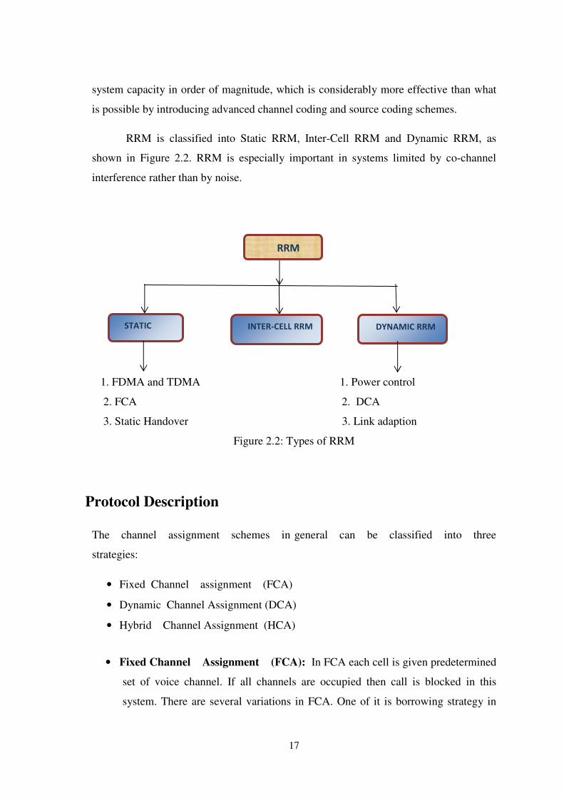
RRM is classified into Static RRM, Inter-Cell RRM and Dynamic RRM, as
shown in Figure 2.2. RRM is especially important in systems limited by co-channel
interference rather than by noise.
1. FDMA and TDMA 1. Power control
2. FCA 2. DCA
3. Static Handover 3. Link adaption
Figure 2.2: Types of RRM
Protocol Description
The channel assignment schemes in general can be classified into three
strategies:
• Fixed Channel assignment (FCA)
• Dynamic Channel Assignment (DCA)
• Hybrid Channel Assignment (HCA)
• Fixed Channel Assignment (FCA): In FCA each cell is given predetermined
set of voice channel. If all channels are occupied then call is blocked in this
system. There are several variations in FCA. One of it is borrowing strategy in
STATIC
RRM
DYNAMIC RRM INTER-CELL RRM
RRM
18
which a cell can borrow channels from neighboring cell which is supervised by
Mobile Switching Center (MSC).
• Dynamic Channel Assignment (DCA): These are more efficient ways of
channel allocation in which voice channels are not allocated to cell permanently .
For every call request from user equipment (UE), base station requests the
channel from MSC. The channel is allocated following an algorithm which
accounts likelihood of future blocking within the cell. It requires the MSC to
collect real time data on channel occupancy, traffic distribution and Radio Signal
Strength Indications (RSSI).
2.2.3 Analytical Model
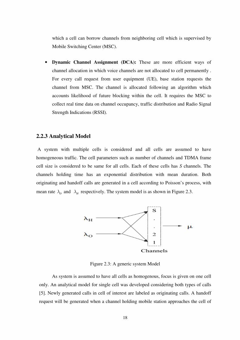
A system with multiple cells is considered and all cells are assumed to have
homogeneous traffic. The cell parameters such as number of channels and TDMA frame
cell size is considered to be same for all cells. Each of these cells has S channels. The
channels holding time has an exponential distribution with mean duration. Both
originating and handoff calls are generated in a cell according to Poisson’s process, with
mean rate Oλ and Hλ respectively. The system model is as shown in Figure 2.3.
Figure 2.3: A generic system Model
As system is assumed to have all cells as homogenous, focus is given on one cell
only. An analytical model for single cell was developed considering both types of calls
[5]. Newly generated calls in cell of interest are labeled as originating calls. A handoff
request will be generated when a channel holding mobile station approaches the cell of

19
interest from its neighboring cell with signal strength below the handoff threshold. In
this model all S channels are shared by both originating and handoff request calls. The
cell handles a handoff request exactly in the same way as an originating call. Both kinds
of requests are blocked if no free channel is available.
With the blocked call clear (BCC) policy, the cell behavior can be described as
(S+I) states Markov process. Each state is labeled by an integer I, (I = 0, 1, 2…S) and it
represents the number of channels in use. The state transition diagram is shown in
Figure 2.4. The system model is modeled as M/M/s/s queuing model.
Figure 2.4: State Transition diagram for system model
Let p be the probability that the system is in state I. the probabilities ( )p i can be
determined in the usual way from birth-death processes. From Figure 2.4 the state
equilibrium is written as in equation (2.1).
0( ) ( 1) 0Hp i p i i si
λ λ
µ
+= − ≤ ≤ (2.1)
Using this equation recursively, along with the normalization condition.
0
( ) 1s
i
p i=
=∑ (2.2)
The steady state probability p(i) is expressed by equation 2.3.
0( ) . (0) 0!
H
ip i p i s
i
λ λ
µ
+= ≤ ≤ (2.3)
Where p (0) is given as,
20
0
0
1(0)
( )
!
is
H
ii
p
i
λ λ
µ=
=+∑
(2.4)
The blocking probability bp for an originating call is given by,
0
0
0
( )
!( )
( )
!
s
H
i
b is
H
ii
ip p S
i
λ λ
µ
λ λ
µ=
+
= =+∑
( 2.5)
The dropping probability is, d bp p= , where bp is calculated by considering the handoff
calls generation rate only ( Hλ ).
2.2.4 Simulation Model
Simulation Formation
The simulation model is designed employing a top-down approach using MATLAB. The
hierarchical structure of network scenarios, users, and processes are provided as
comprehensive developmental environment to model the network. The Discrete Event
simulation method is modeled for all networks under consideration. Simulation model
that is made for analysis is as follows.
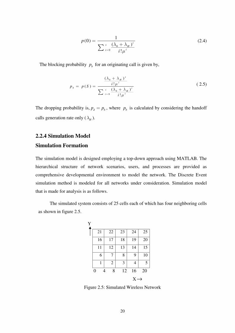
The simulated system consists of 25 cells each of which has four neighboring cells
as shown in figure 2.5.
Y
21 22 23 24 25
16 17 18 19 20
11 12 13 14 15
6 7 8 9 10
1 2 3 4 5
0 4 8 12 16 20
X→
Figure 2.5: Simulated Wireless Network

21
It is assumed that the top cells (Cell 21, 22, 23, 24 and 25) and the bottom cells
(Cell 1, 2, 3, 4 and 5) are connected. It means that if a user comes out of 21 from top, he
will come into cell 1. Analogously, it is assumed that the cells (cell 1, 6, 11, 16 and 21)
and right cells (cell 5, 10, 15, 20 and 25) are connected too.
Handoff-Threshold
Handoff Area
Receive-Threshold
Figure 2.6: Handoff threshold and receive threshold
Assume the base station of each cell is at the center of square. The handoff
threshold can be set at any distance between cell-center to receive-threshold. The area
between handoff-threshold and receive-threshold is called handoff area.(shaded area of
Figure 2.6).
The user movement and distribution within the cell pattern is described as
follows. When a new call request is generated, the location of the mobile users is
random variable, and moving direction is chosen from uniform distribution on the
interval as shown in table 2.1.
Table 2.1. Location and direction of Mobile User
Random Number (0-1) Direction
0-0.25 Target cell is North cell
0.25-0.5 Target cell is East cell
0.5-0.75 Target cell is South cell
0.75-1 Target cell is West cell
The moving speed is uniformly distributed between 8 and 25 m/sec. The user’s
location and RSS is monitored at every second.
22
Radio Propagation Model
Radio propagation is influenced by the path loss depending on the distance, shadowing,
and multipath fading.
The relationship between the transmitted power and received power can be expressed as
below. [2]
100( ) 10 . .P r r P
ξα−= (2.6)
where, ( )P r is the received power; OP is the transmitted power, r is the distance
from the base station to mobile, ξ in decibels has a normal distribution with zero mean
and α is attenuation factor.
Following assumptions are made for simulation
1. Each cell has C=30 channels.
2. Cell radius = 2000 m
3. Arrival of new calls initiating in each cell forms a Poisson’s process with rate λ .
4. Each call requires only one channel for service.
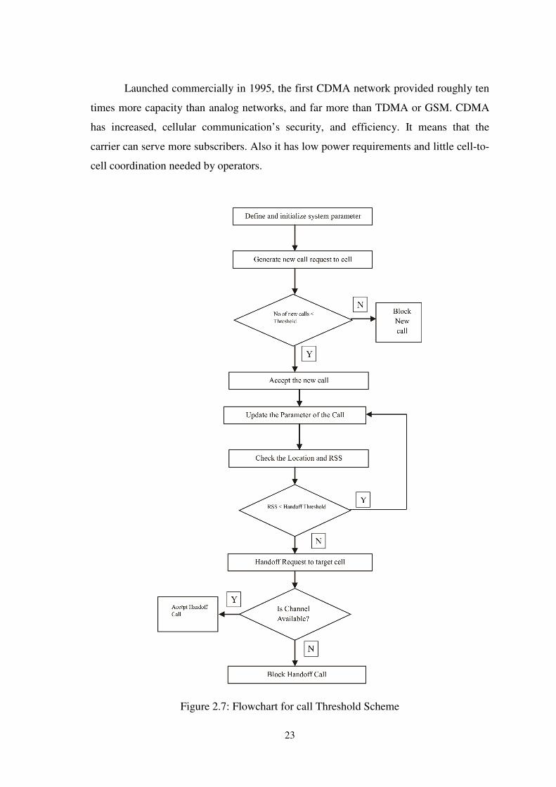
As shown in the flowchart (Figure 2.7), initially call request is generated in the cell,
once a new call is admitted into the network, lifetime of this call is selected according to
its distribution and then total number of new calls is estimated. If channels are accessible
new call is accepted otherwise it is blocked.
Once the call is accepted the parameters of call are updated and signal strength is
checked, if signal strength is less than handoff threshold, at the same time if channel is
available, handoff request is accepted otherwise it is blocked. Thus new blocking
probability and handoff blocking probability is evaluated.
2.3 Code Division Multiple Access (CDMA)
CDMA works on the principle of spread spectrum. With the help of a CODE, data
signal is spread like a noise- like signal which is unable to detect by others. It provides
security as well as noise reduction.
23
Launched commercially in 1995, the first CDMA network provided roughly ten
times more capacity than analog networks, and far more than TDMA or GSM. CDMA
has increased, cellular communication’s security, and efficiency. It means that the
carrier can serve more subscribers. Also it has low power requirements and little cell-to-
cell coordination needed by operators.
Figure 2.7: Flowchart for call Threshold Scheme
24
2.3.1 Adaptive Radio Resource Management in
Hierarchical Cell Structure (HCS)
CDMA system provides large capacity compared with other systems [9]. The most
commonly used methods for increasing capacity are sectorization and microcell
concept, but disadvantage is increased number of handoffs. So, hierarchical cell
structure has been proposed in order to overcome these problems.
In hierarchical cellular system, because mobile users select appropriate cell
layer in accordance with their speed, increase in handoff by fast users, who select
macrocell with large cell size, is solved and capacity is increased by shrinking cell size
for low speed users [44]. Each layer uses its own radio frequency. In these conditions,
spectrum allocation is very important issue, because frequency spectrum is a limited
resource. Since available spectrum is limited in HCS (hierarchical cellular system)
load balancing or resource sharing is needed in order to prevent each layer from being
overloaded.
In order to adapt the changes of traffic, it is necessary to consider adaptive
resource management. Load of each layer in HCS can be balanced by controlling
threshold velocity by which appropriate cell layer is selected [8]. A resource which can
be shared between layers in CDMA based HCS is only Frequency Assignment (FA).
Load of each layer is balanced by changing threshold velocity according to traffic
condition, but when several adjacent microcells are overloaded in rush-hour, overload of
those cells cannot be solved because macrocell does not have enough resources to serve
all overflowed mobile users. In order to overcome this problem, Frequency Borrowing
Resource Allocation (FBRA) scheme is used, but if macrocell does not have enough FA
to support overloaded microcell, this problem cannot be solved [10].
2.3.2 Scheme 1: Static Radio Resource Management (Passive)
In this system, a large number of mobile stations are traversing randomly in the
coverage area of the cell, where two classes of fast and slow mobile stations are
considered. Further it is assumed that a mobile station does not change its speed class
25
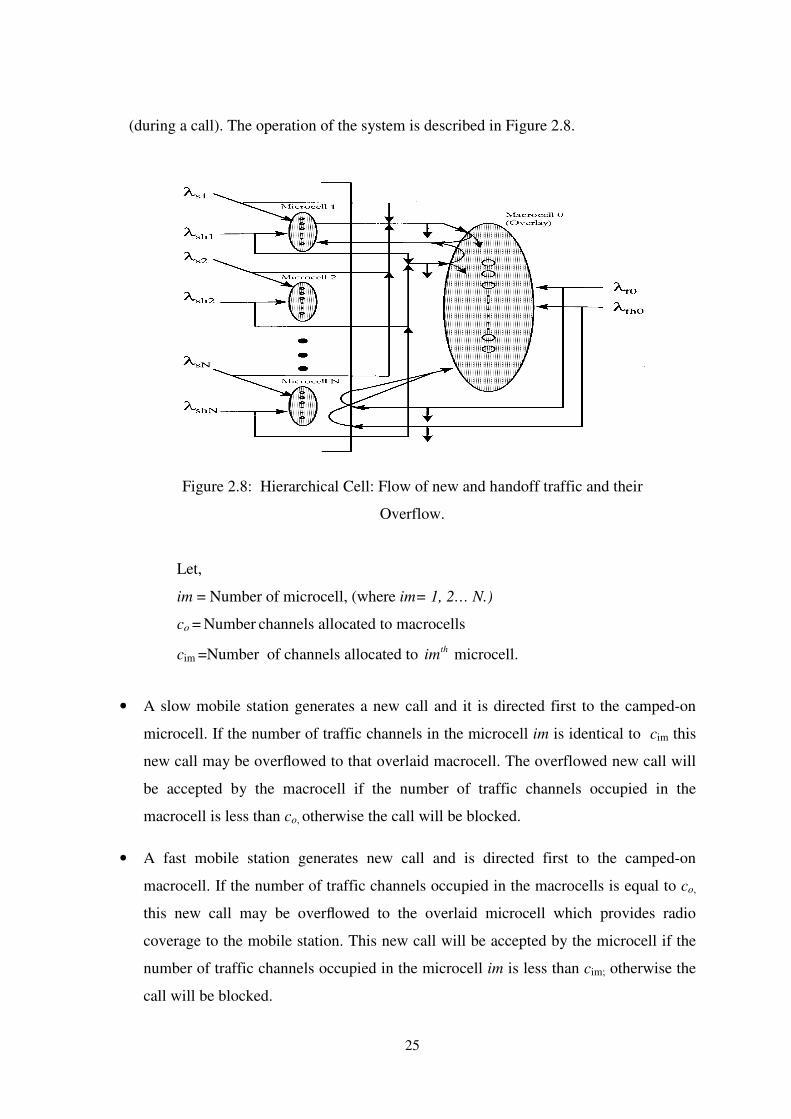
(during a call). The operation of the system is described in Figure 2.8.
Figure 2.8: Hierarchical Cell: Flow of new and handoff traffic and their
Overflow.
Let,
im = Number of microcell, (where im= 1, 2… N.)
co = Number channels allocated to macrocells
cim =Number of channels allocated to thim microcell.
• A slow mobile station generates a new call and it is directed first to the camped-on
microcell. If the number of traffic channels in the microcell im is identical to cim this
new call may be overflowed to that overlaid macrocell. The overflowed new call will
be accepted by the macrocell if the number of traffic channels occupied in the
macrocell is less than co, otherwise the call will be blocked.
• A fast mobile station generates new call and is directed first to the camped-on
macrocell. If the number of traffic channels occupied in the macrocells is equal to co,
this new call may be overflowed to the overlaid microcell which provides radio
coverage to the mobile station. This new call will be accepted by the microcell if the
number of traffic channels occupied in the microcell im is less than cim; otherwise the
call will be blocked.
26
• A handoff request of a slow mobile station is directed first to the target microcell
independent of whether the current serving cell is a neighboring microcell or an
overlaying macrocell. If all traffic channels in the target microcell are busy.
• A handoff request of a fast mobile station is first directed to the target macrocell
independent of whether the current serving cell is a neighboring macrocell or a
neighboring microcell. If all traffic channels in the target macrocell are busy, the
handoff request may be overflowed to the neighboring microcell, which will provide
radio coverage for the mobile station. The overflowed handoff request will be served
by the microcell if there is any idle traffic channel; otherwise, the handoff request will
fail and the call will be forced to terminate (dropped).
Model Description
In this section, system parameters are defined and system model is described. Low and
high mobility mobile stations are two populations of mobile stations. The optimum
spectral efficiency through frequency reuse can be achieved if the traffic of low-
mobility mobile stations is carried by microcell channels and the traffic of high-mobility
mobile stations is carried by macrocell channels, respectively.
The total arriving traffic to the area Ω is denoted byλ . The area under consideration
has one overlaying macrocell and N microcells, im = 1, 2….N. (Figure 2.8). For
simplicity, it is assumed that the microcells are all identical circles with radius 1r and
the macrocells are circles with radius 0r . New traffic solely generated by fast mobile
stations is according to a Poisson process with parameter 0fλ . New traffic solely
generated by slow mobile stations in microcell im, (im = 1, 2…N), is according to a
Poisson process with parametersimλ . The average speed of the slow and fast mobile
subscribers is considered to be SV and fV respectively.
The calls arriving from fast mobile subscribers have overloaded call duration
according to a negative exponential distribution with parameter µ . The unencumbered
call duration is the amount of time that the call would remain in progress without forced
27
termination.
It is assumed that the cell’s dwell time, that is, the time spent by a mobile station
in a cell is a random variable approximated by a negative exponential probability
density function ( pdf ) [44]. For macrocells, the parameters of the exponential pdf for
fast and slow mobile station are denoted by 0η and'
0η respectively. Similarly, for
microcells, the parameters are designated by 1η and '
1η for slow and fast mobile stations,
respectively.
With the above assumptions, the channel occupancy time, that is, the time spent in
a cell by a mobile station being involved in a call, will follow negative exponential
distribution.
For a macrocell, the handoff rate of calls from slow and fast mobile stations is
denoted by '
hoP and hoP respectively, and for a microcell for slow and fast mobile stations
by 1hP and '
1hP , respectively.
The handoff traffic from slow and fast mobile stations in microcell and macrocell
is denoted as follows.
1shλ = Rate of slow mobile station handoff traffic in a microcell.
0'shλ = Rate of slow mobile station handoff traffic in a macrocell.
'
1fhλ = Rate of fast mobile station handoff traffic in a microcell
fhoλ = Rate of fast mobile station handoff traffic in a macrocell.
Performance Analysis
In this section analytical results for the system are presented. During analysis fluid
mobility model is considered. Derivation of slow and fast mobile station’s cell dwell
time in macrocell and microcells is taken into account [44]. Overflow traffic is treated as
Poisson’s distribution and the take -back traffic is delayed until the cell boundary
28
crossing.
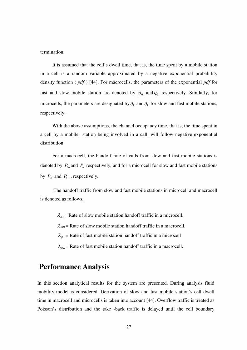
1. In order to obtain the mean channel occupancy time, the mean cell dwell time, or
their inverse, the cell boundary crossing parameters need to be calculated. Using a
fluid flow mobility model, the cell boundary crossing can be derived as follows for
a macrocell [9][10].
0
2
0
fV
rπη = (2.7)
0
2'
0sV
rπη = (2.8)
Where,
0η = Exponential pdf for fast MS in macrocell
` '
0η = Exponential pdf for slow MS in macrocell
sV =Average speed of slow mobile subscribers
fV =Average speed of fast mobile subscribers
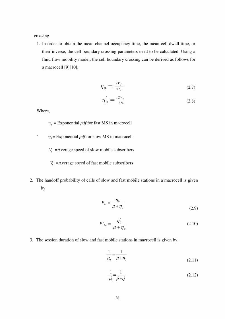
2. The handoff probability of calls of slow and fast mobile stations in a macrocell is given
by
0
0
ηµ
η
+=hoP
(2.9)
'
0
'
0'ηµ
η
+=hoP (2.10)
3. The session duration of slow and fast mobile stations in macrocell is given by,
00
11
ηµµ +=
(2.11)
'
0
''
0
11
ηµµ += (2.12)
29
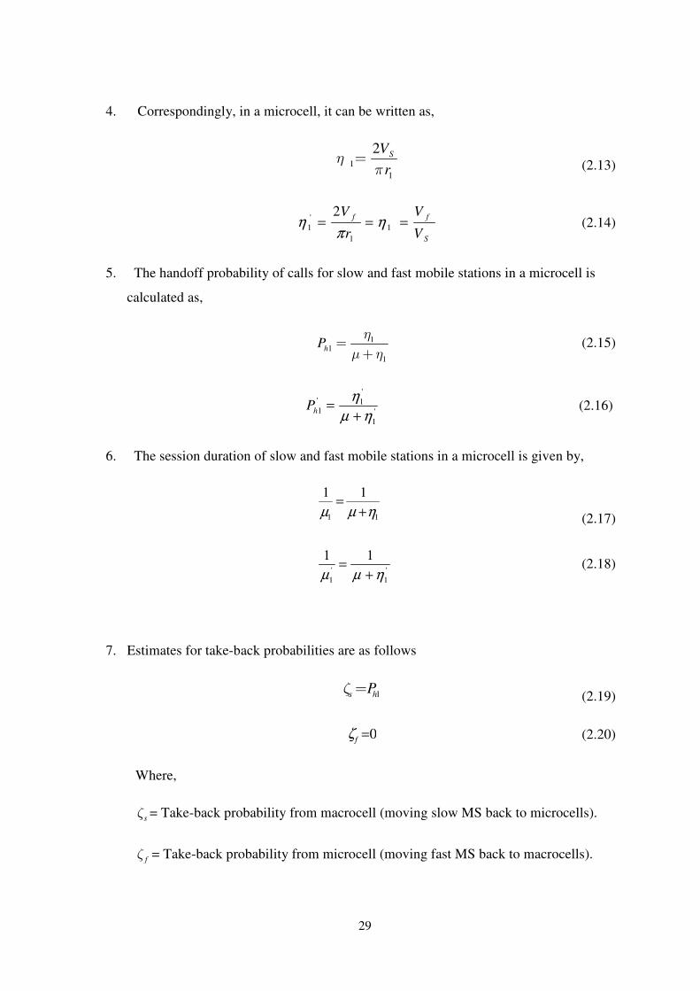
4. Correspondingly, in a microcell, it can be written as,
1
1
2 SV
rη
π=
(2.13)
S
ff
V
V
r
V=== 1
1
'
1
2η
πη (2.14)
5. The handoff probability of calls for slow and fast mobile stations in a microcell is
calculated as,
11
1
hP
η
µ η=
+ (2.15)
'
1
'
1'
1 ηµ
η
+=hP (2.16)
6. The session duration of slow and fast mobile stations in a microcell is given by,
11
11
ηµµ +=
(2.17)
'
1
'
1
11
ηµµ += (2.18)
7. Estimates for take-back probabilities are as follows
1s hPζ =
(2.19)
0=fζ
(2.20)
Where,
sζ = Take-back probability from macrocell (moving slow MS back to microcells).
fζ = Take-back probability from microcell (moving fast MS back to macrocells).

30
Performance Measures
1. The traffic rate to microcells includes the rate of new arrivals )1( 11 bs P−λ and the rate of
accepted handoff traffic )1( 11 bsh P−λ for slow mobile stations and overflow of new
and accepted handoff calls of fast mobile stations from a macrocell, that is,
).1( 100 bbfh PP −λ
2. The aggregate traffic rate into a microcell due to slow mobile stations is as follow:
(2.21)
Where, the take-back traffic rate component is given as
1 1 1 1 1
( ) (1 )sb s sh sb b bo s
P Pλ λ λ λ ζ= + + − (2.22)
3. The aggregate traffic rate into a microcell due to fast mobile stations is given as
( )' '
1 0 1
1t fo fh fbo bo fhP
Nλ λ λ λ λ= + + + (2.23)
4. The generation rate of slow mobile station’s handoff traffic in a microcell is as
follows:
( )( )111111 1 bsbshshsh PP −++= λλλλ (2.24)
5. The generation rate of fast mobile stations’ handoff traffic in a microcell is as
Follows:
' ' ' '
1 1 1 1 1 1 1
1(1 ) (1 ) (1 )fh h fo fho fbo bo b fh b fh bP P P P p
Nλ λ λ λ λ λ
= + + − + − + −
(2.25)
6. The aggregate traffic rate due to fast mobile stations into a macrocell is as follows:
(2.26)
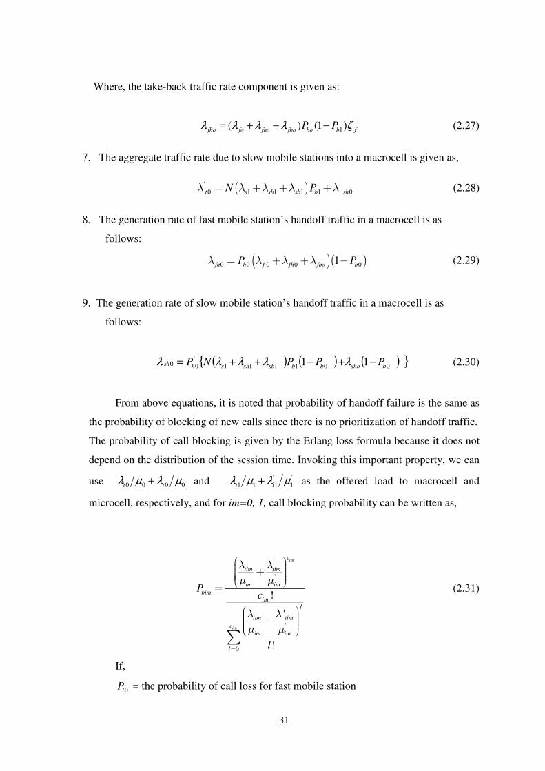
31
Where, the take-back traffic rate component is given as:
1( ) (1 )fbo fo fho fbo bo b f
P Pλ λ λ λ ζ= + + − (2.27)
7. The aggregate traffic rate due to slow mobile stations into a macrocell is given as,
( )' '
0 1 1 1 1 0t s sh sb b shN Pλ λ λ λ λ= + + + (2.28)
8. The generation rate of fast mobile station’s handoff traffic in a macrocell is as
follows:
( )( )0 0 0 0 01fh h f fh fbo bP Pλ λ λ λ= + + − (2.29)
9. The generation rate of slow mobile station’s handoff traffic in a macrocell is as
follows:
) )(( ) ( 0
'
01111
'
00' 11 bshobbsbshshsh PPPNP −+−++= λλλλλ (2.30)
From above equations, it is noted that probability of handoff failure is the same as
the probability of blocking of new calls since there is no prioritization of handoff traffic.
The probability of call blocking is given by the Erlang loss formula because it does not
depend on the distribution of the session time. Invoking this important property, we can
use '
0
'
000 µλµλ tt + and '
1
'
111 µλµλ tt + as the offered load to macrocell and
microcell, respectively, and for im=0, 1, call blocking probability can be written as,
'
'
'
0
!
'
!
im
im
c
tim tim
im im
bimim
l
tim tim
c
im im
l
Pc
l
λ λ
µ µ
λ λ
µ µ
=
+ =
+ ∑
(2.31)
If,
0lP = the probability of call loss for fast mobile station
32
1lP = the probability of call loss for slow mobile station,
then, the probability of of call loss for fast or slow mobile stations is given by
1 0 1lo l b bP P P P= = (2.32)
If no take-back is considered, the probability of call dropping for calls in progress from
fast mobile stations is given as follows:
( )
( )( ) ( )]11][11[
1
]11[ 01
'
1
1
'
110
0
100
bohbh
bhbboh
boh
bbohd
PPPP
PPPPP
PP
PPPP
−−−−
−+
−−≈ (2.33)
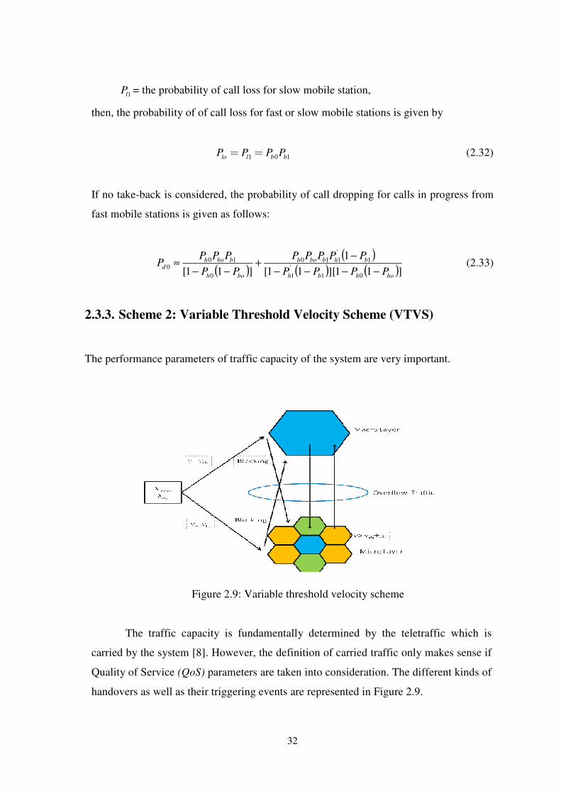
2.3.3. Scheme 2: Variable Threshold Velocity Scheme (VTVS)
The performance parameters of traffic capacity of the system are very important.
Figure 2.9: Variable threshold velocity scheme
The traffic capacity is fundamentally determined by the teletraffic which is
carried by the system [8]. However, the definition of carried traffic only makes sense if
Quality of Service (QoS) parameters are taken into consideration. The different kinds of
handovers as well as their triggering events are represented in Figure 2.9.
33
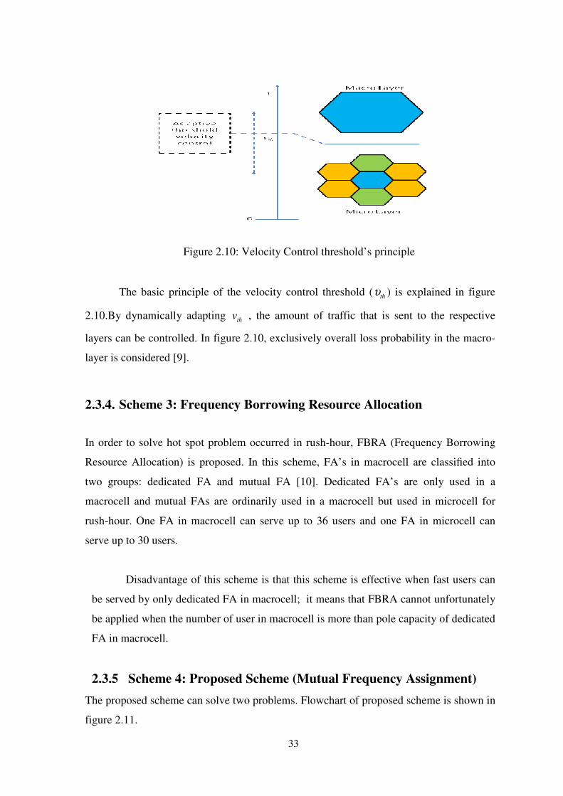
Figure 2.10: Velocity Control threshold’s principle
The basic principle of the velocity control threshold ( thυ ) is explained in figure
2.10.By dynamically adapting thv , the amount of traffic that is sent to the respective
layers can be controlled. In figure 2.10, exclusively overall loss probability in the macro-
layer is considered [9].
2.3.4. Scheme 3: Frequency Borrowing Resource Allocation
In order to solve hot spot problem occurred in rush-hour, FBRA (Frequency Borrowing
Resource Allocation) is proposed. In this scheme, FA’s in macrocell are classified into
two groups: dedicated FA and mutual FA [10]. Dedicated FA’s are only used in a
macrocell and mutual FAs are ordinarily used in a macrocell but used in microcell for
rush-hour. One FA in macrocell can serve up to 36 users and one FA in microcell can
serve up to 30 users.
Disadvantage of this scheme is that this scheme is effective when fast users can
be served by only dedicated FA in macrocell; it means that FBRA cannot unfortunately
be applied when the number of user in macrocell is more than pole capacity of dedicated
FA in macrocell.
2.3.5 Scheme 4: Proposed Scheme (Mutual Frequency Assignment)
The proposed scheme can solve two problems. Flowchart of proposed scheme is shown in
figure 2.11.

34
Figure 2.11: Flowchart of MFA
Microcells
are busy
Microcells can
lend MFA
Microcells has
used MFA
Microcells are
not busy
1th thv v v= −∆ ,
Microcell use MFA
START
12
th thv v v= + ∆
Macrocell uses MFA
2th thv v v= −∆
Microcell use MFA
NN N
NN N
NN N
NN N
NN Y
NN Y
NN Y
NN Y

35
First, when several adjacent microcells are overloaded in rush-hour, over-loads of
those cells can be solved. Second, when more fast users of all dedicated FA’s request
service in macrocell, load of macrocell is decreased by increasing thυ and then microcells
use MFA (Mutual Frequency Assignment). In this case, hand-off between layers occurs
and this is called connect-after-break.
When microcells are overloaded, macrocell should lend microcells MFA, like
scheme 3. FA’s in macrocell are classified into dedicated FA (DFA) and mutual FA
(MFA). When a call is originated, resource in DFA is preferentially assigned and if all
resources in DFA are exhausted, resource in MFA is assigned.
If macrocell is not busy (regardless of use of MFA), macrocell decrease its load by
increasing thυ and then lends microcells MFA. Also, macrocell can control decrease of
load. If macrocell was using MFA, its load is decreased by using 1υ∆ and otherwise, by
using )(2 1υ υ∆ < ∆ .
Consequently, the resource shortage in microcell is solved by increasing the number
of resource and the resource shortage in macrocell is solved by decreasing traffics in
macrocell [46].
Conceptual operation of each scheme, when all calls in macrocells are assigned in
only DFA is described in Figure 2.12. Utilization of resource is given by RU and
defined as,
RU = the number of user / pole capacity of cell
In scheme 1, RU of microcells will increase with load of microcells and in scheme 2,
for a little while, load of microcell will be stabilized by increasing thυ ,but load of
macrocell will increase and thus be rapidly saturated as shown in Fig 2.13. In this case,
since MFA in macrocell is not used, scheme 3 and scheme 4 show superior
performance.
36
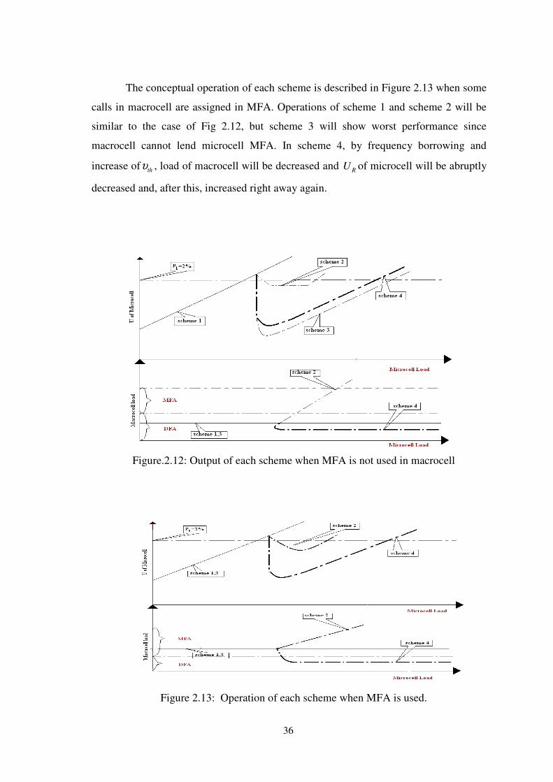
The conceptual operation of each scheme is described in Figure 2.13 when some
calls in macrocell are assigned in MFA. Operations of scheme 1 and scheme 2 will be
similar to the case of Fig 2.12, but scheme 3 will show worst performance since
macrocell cannot lend microcell MFA. In scheme 4, by frequency borrowing and
increase of thυ , load of macrocell will be decreased and RU of microcell will be abruptly
decreased and, after this, increased right away again.
Figure.2.12: Output of each scheme when MFA is not used in macrocell
Figure 2.13: Operation of each scheme when MFA is used.
37
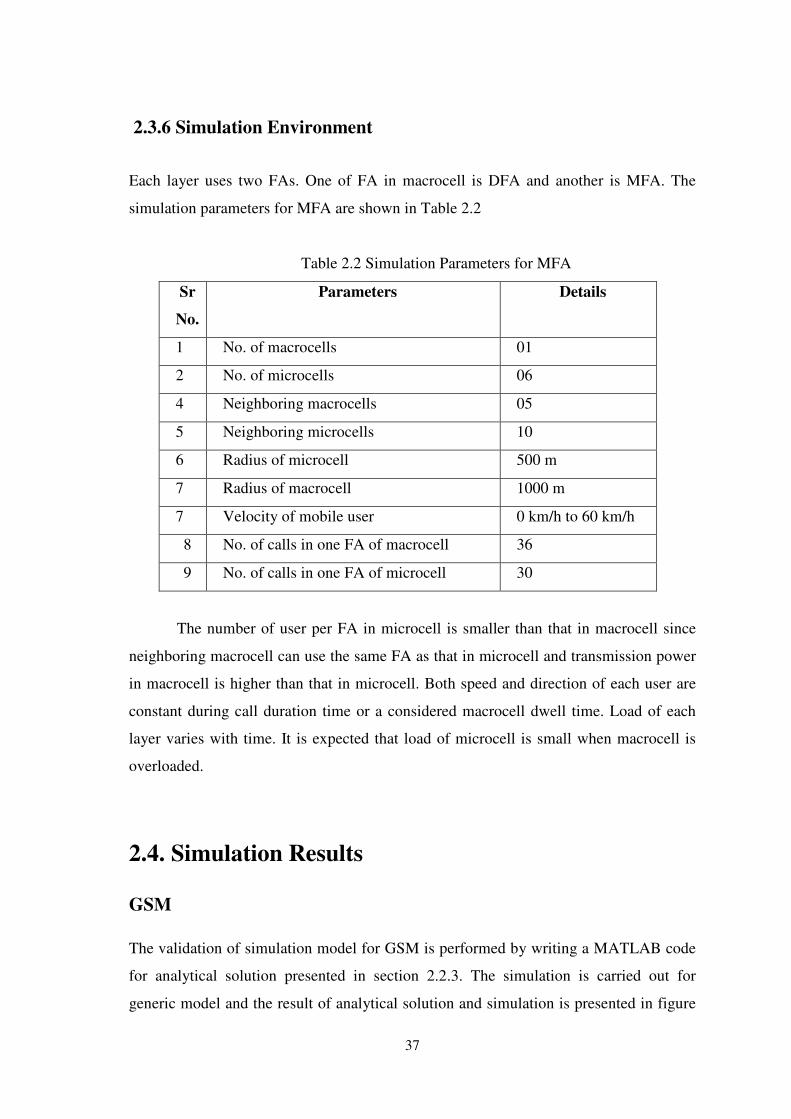
2.3.6 Simulation Environment
Each layer uses two FAs. One of FA in macrocell is DFA and another is MFA. The
simulation parameters for MFA are shown in Table 2.2
Table 2.2 Simulation Parameters for MFA
Sr
No.
Parameters Details
1 No. of macrocells 01
2 No. of microcells 06
4 Neighboring macrocells 05
5 Neighboring microcells 10
6 Radius of microcell 500 m
7 Radius of macrocell 1000 m
7 Velocity of mobile user 0 km/h to 60 km/h
8 No. of calls in one FA of macrocell 36
9 No. of calls in one FA of microcell 30
The number of user per FA in microcell is smaller than that in macrocell since
neighboring macrocell can use the same FA as that in microcell and transmission power
in macrocell is higher than that in microcell. Both speed and direction of each user are
constant during call duration time or a considered macrocell dwell time. Load of each
layer varies with time. It is expected that load of microcell is small when macrocell is
overloaded.
2.4. Simulation Results
GSM
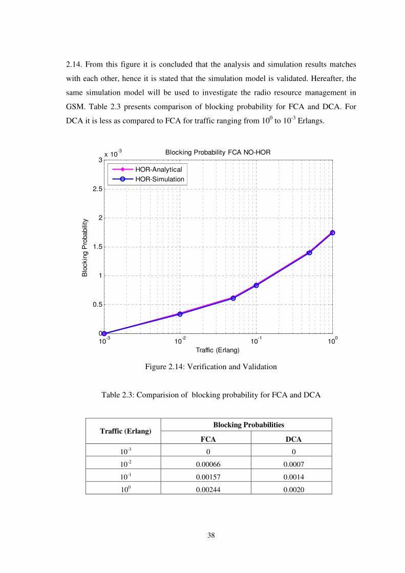
The validation of simulation model for GSM is performed by writing a MATLAB code
for analytical solution presented in section 2.2.3. The simulation is carried out for
generic model and the result of analytical solution and simulation is presented in figure
38
2.14. From this figure it is concluded that the analysis and simulation results matches
with each other, hence it is stated that the simulation model is validated. Hereafter, the
same simulation model will be used to investigate the radio resource management in
GSM. Table 2.3 presents comparison of blocking probability for FCA and DCA. For
DCA it is less as compared to FCA for traffic ranging from 100 to 10
-3 Erlangs.
10-3
10-2
10-1
100
0
0.5
1
1.5
2
2.5
3x 10
-3
Traffic (Erlang)
Blo
ckin
g P
robabili
ty
Blocking Probability FCA NO-HOR
HOR-Analytical
HOR-Simulation
Figure 2.14: Verification and Validation
Table 2.3: Comparision of blocking probability for FCA and DCA
Traffic (Erlang) Blocking Probabilities
FCA DCA
10-3
0 0
10-2
0.00066 0.0007
10-1
0.00157 0.0014
100 0.00244 0.0020
39
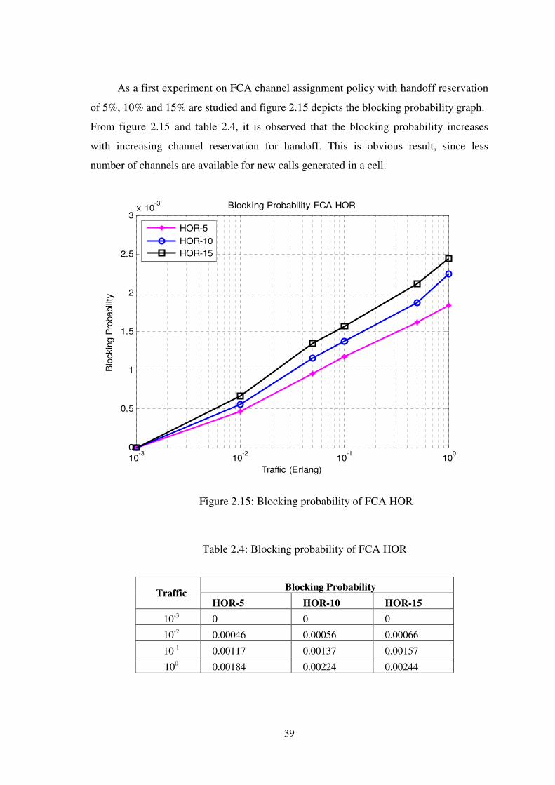
As a first experiment on FCA channel assignment policy with handoff reservation
of 5%, 10% and 15% are studied and figure 2.15 depicts the blocking probability graph.
From figure 2.15 and table 2.4, it is observed that the blocking probability increases
with increasing channel reservation for handoff. This is obvious result, since less
number of channels are available for new calls generated in a cell.
10-3
10-2
10-1
100
0
0.5
1
1.5
2
2.5
3x 10
-3
Traffic (Erlang)
Blo
ckin
g P
robabili
ty
Blocking Probability FCA HOR
HOR-5
HOR-10
HOR-15
Figure 2.15: Blocking probability of FCA HOR
Table 2.4: Blocking probability of FCA HOR
Traffic Blocking Probability
HOR-5 HOR-10 HOR-15
10-3
0 0 0
10-2
0.00046 0.00056 0.00066
10-1
0.00117 0.00137 0.00157
100 0.00184 0.00224 0.00244

40
The second performance metric for RRM assessment is dropping probability.
Figure 2.16 shows the dropping probability graph for FCA.
It is observed that for 15% reservation the dropping probability is lowest as compared to
10% and 5% reservation. (Table 2.5)
10-3
10-2
10-1
100
10-7
10-6
10-5
10-4
Call Arrival Rate
Dro
pin
g P
robabili
ty
Call Arrival Rate Vs dropping Probability FCA HOR
HOR-5
HOR-10
HOR-15
Figure 2.16: Call Arrival VS Dropping probability of FCA
Further investigation in GSM system is performed for radio resource
management in a dynamic channel assignment. The simulation results for DCA with
handoff channel reservation are shown in figure 2.17 and 2.18; for blocking and
dropping probabilities respectively. From figure 2.17 it is observed that the performance
of GSM from DCA is equivalent to FCA but there is some improvement in the blocking
probability.

41
Table 2.5: Dropping probability of FCA
10-3
10-2
10-1
100
0
0.5
1
1.5
2
2.5
3x 10
-3
Traffic (Erlang)
Blo
ck
ing
Pro
ba
bil
ity
Blocking Probability DCA HOR
HOR-5
HOR-10
HOR-15
Figure 2.17: Blocking probability of DCA HOR
Table 2.6: Blocking probability of DCA HOR
Call Arrival Rate Dropping Probability
HOR-5 HOR-10 HOR-15
10-3
0.0000001675 0.0000001475 0.0000001175
10-2
0.000001135 0.000000735 0.000000535
10-1
0.000008465 0.000005465 0.000003465
100 0.00006885 0.00003885 0.00002785
Call Arrival Rate Blocking Probability
HOR-5 HOR-10 HOR-15
10-3
0 0 0
10-2
0.00034 0.00050 0.0007
10-1
0.0009 0.00114 0.0014
100 0.0016 0.0018 0.0020
42
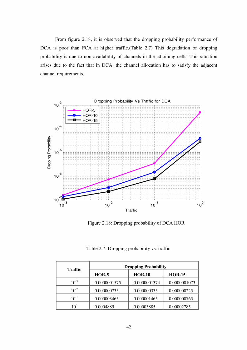
From figure 2.18, it is observed that the dropping probability performance of
DCA is poor than FCA at higher traffic.(Table 2.7) This degradation of dropping
probability is due to non availability of channels in the adjoining cells. This situation
arises due to the fact that in DCA, the channel allocation has to satisfy the adjacent
channel requirements.
10-3
10-2
10-1
100
10-7
10-6
10-5
10-4
10-3
Traffic
Dro
pin
g P
robability
Dropping Probability Vs Traffic for DCA
HOR-5
HOR-10
HOR-15
Figure 2.18: Dropping probability of DCA HOR
Table 2.7: Dropping probability vs. traffic
Traffic Dropping Probability
HOR-5 HOR-10 HOR-15
10-3
0.0000001575 0.0000001374 0.0000001073
10-2
0.000000735 0.000000335 0.000000225
10-1
0.000003465 0.000001465 0.000000765
100 0.0004885 0.00003885 0.00002785
43
CDMA
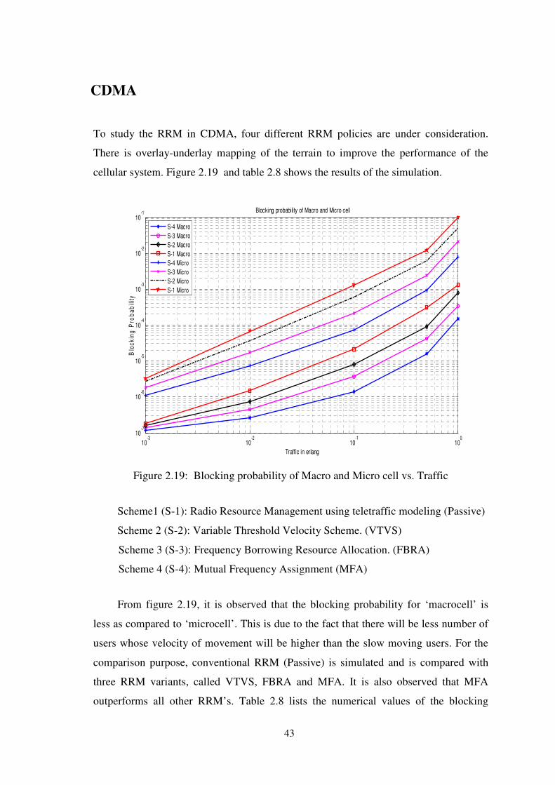
To study the RRM in CDMA, four different RRM policies are under consideration.
There is overlay-underlay mapping of the terrain to improve the performance of the
cellular system. Figure 2.19 and table 2.8 shows the results of the simulation.
10-3
10-2
10-1
100
10-7
10-6
10-5
10-4
10-3
10-2
10-1
Traffic in erlang
Blo
ck
ing
Pro
ba
bil
ity
Blocking probability of Macro and Micro cell
S-4 Macro
S-3 Macro
S-2 Macro
S-1 Macro
S-4 Micro
S-3 Micro
S-2 Micro
S-1 Micro
Figure 2.19: Blocking probability of Macro and Micro cell vs. Traffic
Scheme1 (S-1): Radio Resource Management using teletraffic modeling (Passive)
Scheme 2 (S-2): Variable Threshold Velocity Scheme. (VTVS)
Scheme 3 (S-3): Frequency Borrowing Resource Allocation. (FBRA)
Scheme 4 (S-4): Mutual Frequency Assignment (MFA)
From figure 2.19, it is observed that the blocking probability for ‘macrocell’ is
less as compared to ‘microcell’. This is due to the fact that there will be less number of
users whose velocity of movement will be higher than the slow moving users. For the
comparison purpose, conventional RRM (Passive) is simulated and is compared with
three RRM variants, called VTVS, FBRA and MFA. It is also observed that MFA
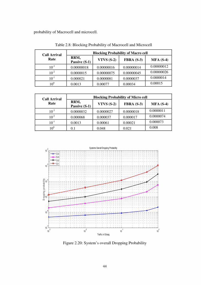
outperforms all other RRM’s. Table 2.8 lists the numerical values of the blocking
44
probability of Macrocell and microcell.
Table 2.8: Blocking Probability of Macrocell and Microcell
Call Arrival
Rate
Blocking Probability of Macro cell
RRM,
Passive (S-1) VTVS (S-2) FBRA (S-3) MFA (S-4)
10-3
0.00000018 0.00000016 0.00000014 0.00000012
10-2
0.0000015 0.00000075 0.00000045 0.00000026
10-1
0.000021 0.0000081 0.0000037 0.0000014
100 0.0013 0.00077 0.00034 0.00015
Call Arrival
Rate
Blocking Probability of Micro cell
RRM,
Passive (S-1) VTVS (S-2) FBRA (S-3) MFA (S-4)
10-3
0.0000032 0.0000027 0.0000018 0.0000011
10-2
0.000068 0.000037 0.000017 0.0000074
10-1
0.0013 0.00061 0.00021 0.000073
100 0.1 0.048 0.021 0.008
10-3
10-2
10-1
100
10-7
10-6
10-5
10-4
10-3
10-2
Traffic in Erlang
Dro
pp
ing
pro
ba
bil
ity
Systems Overall Dropping Probability
S-4
S-3
S-2
S-1
Figure 2.20: System’s overall Dropping Probability

45
Figure 2.20 shows the results of systems overall dropping probability in case of
all the RRM’s as mentioned earlier. It is observed that MFA results in better
performance than the other three RRM’s (table 2.9).
Table 2.9: Dropping probability of overall system.
Traffic(Erlang) System overall Dropping Probability
RRM,
Passive(S-1) VTVS (S-2) FBRA (S-3)
MFA (S-4)
10-3
0.000014 0.0000051 0.000002 0.0000005
10-2
0.000041 0.0000102 0.0000038 0.00000065
10-1
0.00012 0.000032 0.000008 0.00000088
100 0.0011 0.0003 0.000061 0.0000022
It is also observed that the variation of dropping probability with respect to change
in traffic is very low as compared to other three schemes. This is due to the fact that the
velocity threshold is dynamically adjusted in accordance with the traffic conditions.
2.5 Conclusion
2.5.1 GSM
1. Performance of FCA and DCA is evaluated. The blocking and dropping
probabilities are calculated for reservation of channels for handoff calls. From the
analysis and simulation carried out, it can be concluded that dropping probability
for HO-reservation of 15% channels is best. The results of simulation and an
analytical model indicate that as there is increase in percentage of priority
channels, dropping probability reduces.
2. It is necessary to keep both, cochannel interference and adjacent channel
interference, under a certain threshold. This is achieved by restricting cells within
the required minimum channel reuse distance from a cell that borrows a channel
from the central pool, DCA also requires fast real-time signal processing and
associated channel database updating.
46
2.5.2 CDMA
1. A new adaptive radio resource management scheme is proposed in CDMA
based hierarchical cell structure i.e. MFA [8] [9]. In this scheme, the resource
shortage in microcell is solved by increasing the number of resource and the
resource shortage in macrocell is solved by decreasing traffic in macrocell. One
of the notable features in the proposed scheme is to increase threshold velocity
rather than to decrease threshold velocity when most channels in microcell are
busy.
2. Thus, abrupt increase of macrocell load caused by decreasing threshold velocity
when microcell is overloaded can be solved. Although the number of handoff is
increased in this case, the number of call loss can be decreased since this
problem occurs during only rush-hour. In other words, call could be prevented
from dropping or blocking although handoff rate is increased slightly. It is
revealed that this proposed scheme MFA, considerably improves call dropping,
call blocking and utilization of resource.


