
Micro-pulse Lidar Signals: Uncertainty Analysis
Submission to Journal of Atmospheric and
Oceanic Technology: Notes and Correspondence
Elltsworth J. Welton 1 and James R. Campbell 2
° Goddard Earth Sciences and Technology Center
University of Maryland Baltimore County
Baltimore, Maryland 21250 USAPh: 301-614-627!)
Fax: 301-614-5492
Email: welton@ virl.gsfc.nasa.gov
° Science Systems and Applications, Inc.
Lanham, Maryland 20706 USAPh: 301-614-62713
Fax: 301-614-54!)2
Email: campbell@ virl.gsfc.nasa.gov
https://ntrs.nasa.gov/search.jsp?R=20020060463 2018-05-19T03:31:05+00:00Z

5 qqJ8
December 20, 2001
Micro-pulse Lidar Signals: Uncertainty Analysis
Authors:
Ells.worth J. Welton ° and James R. Campbell
Submission to the Journal of Atmospheric and Oceanic Technology
Micro-pulse lidar (/VlPL) systems are small, autonomous, eye-safe lidars used for
continuous observations of the vertical distribution of cloud and aerosol layers. Since the
construction of the first MPL in 1993, procedures have been developed to correct for various
instrument effects present in MPL signals. The primary instrument effects include afterpulse,
laser-detector cross-talk, and overlap, poor near-range (< 6 km) focusing. The accurate
correction of both afterpulse and overlap effects are required to study both clouds and aerosols.
Furthermore, the outgoing energy of the laser pulses and the statistical uncertainty of the MPL
detector must also be correctly determined in order to assess the accuracy of MPL observations.
The MPL-Net project at GSFC coordinates the deployment of MPL instruments to sites
co-located with AERONET sunphotometers. The raw MPL data is downloaded to a central
archive and processed to correct for the various instrument effects discussed above. A paper that
describes the techniques used to correct the raw MPL data has been accepted for publication by
the Journal of Atmospheric and Oceanic Technology. However, the paper did not discuss the net
uncertainty in the corrected MPL-Net data product.
This new paper discu,;ses the uncertainties in the determination of the afterpulse, overlap,
pulse energy, detector noise, and all remaining quantities affecting measured MPL signals. The
uncertainties are propagated through the entire correction process to give a net uncertainty on the
final corrected MPL-Net data product. The results show that in the near range, the overlap
uncertainty dominates. At altitudes above the overlap region, the dominant source of uncertainty
is caused by uncertainty in the pulse energy. However, if the laser energy is low, then during
mid-day, high solar background levels can significantly reduce the signal-to-noise of the
detector. In such a case, the statistical uncertainty of the detector count rate becomes dominant at
altitudes above the overlap region.
* Lead Author: Dr. Ellsworth J. Welton
Goddard Earth Sciences and Technology Center, UMBCGSFC Code 912
welton @ virl.gsfc.nasa, gov

Abstract
Micro-pulse lidar (MPL) systemsare small, autonomous,eye-safe lidars used for
continuousobservationsof' the vertical distribution of cloud and aerosol layers. Since the
constructionof the first MPL in 1993,procedureshavebeendevelopedto correct for various
instrumenteffectspresentin MPL signals.The primary instrumenteffects include afterpulse,
laser-detectorcross-talk, and overlap, poor near-range (< 6 km) focusing. The accurate
correctionof bothafterpulseandoverlapeffectsarerequiredto studybothcloudsandaerosols.
Furthermore,theoutgoingenergyof the laserpulsesandthe statisticaluncertaintyof the MPL
detectormustalsobecorrectlydeterminedin orderto assesstheaccuracyof MPL observations.
The uncertaintiesassociatedwith the afterpulse,overlap,pulseenergy,detectornoise,and all
remaining quantities affec_LingmeasuredMPL signals, are determined in this study. The
uncertaintiesarepropagatedthroughtheentireMPL correctionprocessto give a net uncertainty
on the final corrected MPL signal. The results show that in the near range, the overlap
uncertaintydominates.At altitudesabovetheoverlapregion,thedominantsourceof uncertainty
is causedby uncertaintyin the pulseenergy.However, if the laser energyis low, then during
mid-day, high solar backgroundlevels can significantly reducethe signal-to-noise of the
detector.In sucha case,the :_tatisticaluncertaintyof thedetectorcountratebecomesdominantat
altitudesabovetheoverlapregion.
1. Introduction
During the 1990s technological advances made possible the development of compact,
autonomous, and eye-safe lidar systems. The Micro-pulse Lidar (MPL) was the first of this new
class of instruments (SpinhJtrne, 1993; Spinhirne et al., 1995). The MPL has since been used
successfully within the Atmospheric Radiation Measurement (ARM) program (Stokes and
Schwartz 1994), and also in several independent field experiments around the world (Welton et
al., 2000; Peppler et al., 2000; Voss et al., 2001; Welton et al., 2001). An overview of the MPL
instruments operated with!in the ARM program is discussed by Campbell et al. (2001),
henceforth referred to as CA.
Welton et al. (2000) and CA discuss the nature of the measured MPL signal with respect
to the lidar equation (Femald et al., 1972). The measured signals are shown to differ from the
theoretical lidar equation because of specific effects caused by the MPL transmit/receive optical
design. Both Welton et al. _ad CA develop correction factors for each instrument-related effect,
and present algorithms that convert the measured signal into a form that complies with the lidar
equation.
The two algorithms differ in their approach to the correction process. The earlier
algorithm by Welton et al. determined the correction factors by forcing measured signals to
conform to a modeled lidar signal containing only molecular scattering. However, this method is
only useful when measurements can be conducted in regions free of aerosols and clouds, such as
on mountain-tops. The CA algorithm is not dependent upon this condition, and is more
applicable to most field conditions. Also, the CA algorithm is more rigorous in its construction,
and is better suited to understanding the uncertainties involved in the correction process. For
these reasons, an adapted version of the CA algorithm was used by Welton et al. (2001) for
2
processingMPL data from a later field experiment. The authors intend to utilize the CA
algorithm for future studies.
This paper presents a study of the uncertainties associated with the correction factors
discussed by CA. The uncertainties are propagated through the CA algorithm to yield a net
uncertainty in the final conw_rted MPL signal.
2. The MPL Signal
This section describes the terms that are present in the lidar equation. Figure 1 shows an
example of MPL observed p]hoton count rates during both day and night. The MPL count rate is
presented as Equation 2 in CA, and is rewritten here as
A,aw(r,E) BrawPraw(r) = CEO(r)i[flM(r) + flp(r)]TM2(r)Tp2(r) + ÷ (1)
D(P=.)r 2 D(Pra_) D(P_.)
where P_aw(r) is the measured signal (photoelectrons/_sec per shot) at range r, C is a calibration
value, E is the pulse energy in laJ, D(Praw) is the detector dead-time factor, O(r) is the overlap
function, A(r,E) is the detector afterpulse (photoelectrons/I.tsec per shot), and B is the solar
background signal (photoelectrons/I.tsec per shot).
Normalized Relative Backscatter Signals
The backscatter cross-section terms, [3M(r) and ]3e(r), in Eq. (1) are due to molecules and
particles, respectively. Sources of particle backscatter include clouds, aerosols, or a mixture of
both. The transmission terms, TM2(r) and Tp2(r), are given by

Is;o, ]T_Z(r) = exp -2 (r')dr" (2)
where o(r) is the extinction coefficient, and the i subscript denotes either a molecular or particle
quantity. The integral of the extinction coefficient from the MPL to any range is the optical depth
over that distance. The transmission terms are squared to account for the two-way path of the
laser pulses.
The aim of the CA correction algorithm is to remove all instrument parameters from Eq.
(1) except C, and to subtrac, t B. The signal resulting from the correction process is called the
normalized-relative-backscatter signal, henceforth referred to as the NRB signal. The NRB
signal, PSRB(r), is given by
P_Rs(r) = C[& (r) + flp(r)]TM2(r)Tp2(r) (3)
The NRB signal is significaJat because it is dependent on atmospheric parameters and only one
instrument parameter, C. Techniques to determine C using measured NRB signals are well
understood and are independent of the lidar system (Spinhirne et a1.,1980; Welton et al., 2001).
Detector Dead-time Corrections
The first step in processing the MPL signals is to correct for detector dead-time effects.
Dead-time effects are caused by saturation of the detector signals at high count rates and are
discussed in detail by CA. Here we attempt to quantify the uncertainty in the dead-time
correction based on information provided by the manufacturer and others with expertise in the
field of photon counting detectors (X. Sun, personal communication).
The dead-time factor is determined using the following equation,
4

D(p,.aw)= _ (4)P_,,A
where Z is a calibrated source signal, A is the total attenuation of the optical path from the source
to the detector, and P_,,, is the observed photon count rate. The uncertainty in D(P_,w) is given by,
6D(Pr_) = D(P_w) +[A_---")(5)
where _YXand 5P_w are the uncertainties in the source and measured signals, respectively, and are
determined using Poisson statistics. _iA is the uncertainty in the attenuation term. The
uncertainties in each signal term are estimated assuming a per second count rate with no time
average. The source uncertainty was well below 1% and was negligible. The attenuation
uncertainty was ignored in order to assess the uncertainty in the dead-time caused by fluctuations
in the source and measured ,;ignal.
Figure 2a shows a plot of D(Praw) versus the measured count rate, Pra,,. Figure 2b shows
5D(P,_w)/D(Pr,w) versus D(P_,w). The dead-time uncertainty is negligible at high count rates but
approaches 1% at low count rates because the detector uncertainty is highest when the count rate
is low. However, the dead-time factor itself is only significant for values above 1.01, the level at
which the measured signals are affected by at least 1% due to dead-time effects. At dead-time
factors above 1.01, the dead-time uncertainty is less than 0.3%. As a result, the source and
measured signal uncertainties contribute very little to the overall dead-time uncertainty. Instead,
the uncertainty in the dead-time factor is dependent almost entirely on the uncertainty in the
5

attenuationoptic. The attenuationuncertaintyis not know at this time. For thepurposesof this
study,wewill considerthis to besmallandtheoverall dead-timeuncertaintyto benegligible.
Thedead-timecorrectedlidar signal,P(r), is givenby
P(r) = EO(r) PN_ (r)2 + A(r, E) + B (6)r
Using Poisson statistics, the uncertainty in P(r) is
_ p(r) = _P___ ) (7)
where N is the number of shots during the acquisition of the signal and is dependent on the data
rate. N is typically either 75,000 for a 30 second data rate, or 150,000 for a 1 minute data rate.
Figure 1 shows the uncertainty in the observed count rate. Also, the error in B is given by Eq.
(7), but is done using the signal returns from 45 to 55 km as discussed by CA.
Uncertainties in the Laser Energy
A portion of the outgoing laser pulse energy is measured in real-time by another detector,
the energy monitor. A calibration table is used to calculate the actual pulse energy from the
energy monitor value. The relationship between the two is linear. The calibration table does not
have to be very accurate in terms of generating the true output energy. Instead, it only has to
provide an output energy that is proportional to the actual value because any constant offset in
the energy term can be passed to the calibration value, C. Henceforth, the term energy monitor
value refers to the calibrated pulse energy, not the actual pulse energy.
6

Theaverageenergymonitorvalueduring themeasurementperiod (typically 1minute) is
storedin theMPL datafile. Changesin theenergymonitor valuefrom pulseto pulseduring the
measurementperiod will produceuncertainty in the energy value. If the energy uncertainty
becomeshighit candominatethe uncertaintyin theMPL signal.Therefore,the energymonitor
valuemustbecarefullyconsidered.
The energymonitor value canchangefrom pulse to pulsedue to changesin the laser
powersetting,degradationof the laserdiodeover time, changesin beamquality outputfrom the
laserhead,and statistical fluctuationsin the energymonitor. The laserpower setting is fixed
during operationof the MPL. Therefore,the diode power will only drop if the laser system
beginsto degrade,howeverthis takesplaceovera long time spanand will not producepulseto
pulsechangesin theenergyunlessacatastrophicfailure occurs.Thelaserheadcomponentsmay
alsodegradewith time, butagainthis will not producesignificantpulseto pulsechangesunless
the laser headbreaks.The beamquality may be affected by environmentalchangessuchas
increaseor decreasein temperatureandhumidity of the lasercomponents.This could occurover
much smaller time frames and is considereda possible source of uncertainty. Statistical
fluctuations in the energymonitor are also considereda sourceof uncertainty. In addition,
temperaturechangeson the energymonitor produceanothersourceof uncertaintybecauseof
thermalnoisein thedetector.
The uncertainty in the energy monitor value was determined using the following
procedure.Data from five MPL systemswere collected. Table 1 showsthe averageenergy,
percentenergyfluctuation, averagetemperature,and percenttemperaturefluctuation of each
MPL systemoverM numberof minutesof data.Theenergymonitor valuesrangefrom 3.71 to
7.64 I-tJandthe temperaturevaluesrangefrom 26.93° to 30.55° C betweenthe MPL systems
7

picked for this study.MPL systemshavevarying degreesof laser quality due to age,andthis
rangeof energycoversthetypical spanfound in mostMPL systems.Also, thetemperaturerange
coversthe typical spanencounteredduring most MPL operations.Figure 3 showsthe percent
fluctuationin energyversusthepercentfluctuationin temperaturefor thefive MPL systems.The
datashow that whenthe changein temperatureis low, the percentfluctuation in the energy
monitor valueis approximately1%or less.When thechangein temperatureis low, theprimary
sourceof energychangeis simply statisticalfluctuation within the detector.Typical MPL data
acquisitionratesare1minuteor lessandtemperaturechangesarenegligibleoversuchshorttime
spansunless there is a noticeable problem with the instrument. Therefore, under normal
conditionstheuncertaintyin theenergymonitor valueis setconstantto 1%for all MPL systems.
However,if thedatarate is increasedto severalminutesor more,then temperaturefluctuations
affectingtheenergyuncertaintyshouldbeconsidered.
3. Afterpulse Corrections
The next step in MPL processing is the afterpulse correction. A complete discussion of
afterpulse is given by CA, a brief description is given here. The initial firing of each laser pulse
is seen by the detector because the MPL shares the same transmit and receive path. The initial
pulse on the detector is large and creates a false signal on the detector as the photoelectrons are
bled off. This false signal must be removed from the measured signals by pre-determining
A(r,E), and then subtracting it from P(r). This process is referred to as afterpulse correction and
is discussed here. A(r,E) is determined by covering the MPL and preventing signals from being
transmitted. In this arrangement, the first term on the right-hand-side (RHS) of Eq. (6) is zero,
and the detector only measures the afterpulse signal and background. The background is only

equalto the detector dark noise with the lid on. The afterpulse is dependent upon the output
energy and according to CA is written as
A(r, Ea):= EAAN(r) (8)
where Ea is the energy monitor value during the afterpulse measurement.
AN(r) is referred to as the normalized afterpulse. In order to measure AN(r), the dark noise
is subtracted from P(r) and the result is divided by EA. As(r) is given by
AN(r ) _ A(r) = P(r)-B o (9)
where B D is the detector dark noise. This measurement is performed for a certain period of time
(typically about 10 minutes). AN(r) is the average of the signals over the time span, and the
afterpulse uncertainty, 8A(r), is
I t_P(r) 2 t_(SEa ] 2tSAN(r ) = A_(r) [P(r)- B] 2 _. E,t J(10)
where SEa is the uncertainty in the outgoing energy during the afterpulse measurement. Figure 4a
shows a typical afterpulse function versus range, and Figure 4b shows the afterpulse uncertainty.
Signals measured during regular operations are corrected by subtracting EAN(r) from
[P(r)-B] and then dividing by E. However, B and E are the values taken during the regular
9
measurement,not
P_A(r),is givenby
the aftecpulsemeasurement.The normalized-afterpulse-correctedsignal,
P(r)- B- [EA_(r)] _ O(r)P_nz (r) (11)PNA(r) =E r 2
4. Overlap Corrections
The next step in MPL processing is the overlap correction. A complete discussion of
overlap is given by CA, a brief description is given here. The overlap function accounts for
signal loss in the near-range due to poor receiver efficiency of the telescope and associated optics
in this region. The overlap problem must be corrected in order to analyze boundary layer
aerosols. The CA overlap correction process involves acquiring MPL data while the instrument
is oriented horizontally. In this arrangement, both 13and _ are constant with range. Using Eq. (3)
and multiplying Eq. (11) by r2 gives the resulting horizontal MPL signal
PH(r) = C,B O(r) exp[-2or] (12)
The natural logarithnl of Eq. (12) is
ln[PH(r) ] := In[Cfl] + ln[O(r)]- 2or (13)
At distances greater than the overlap range, O(r) is equal to one and the second term on the RHS
of Eq. (13) is zero. In this region, ln[P_A(r)] is linear with respect to range. A least squares linear
10
fit is appliedto N data points from ro to a maximum range, rm_,. The maximum range is typically
about 2 km greater than re. The resulting linear fit is given by
ln[PF(r)] = In[C/3]- 2or (14)
where the y-intercept is ln[CI3] and the slope is -2_. The overlap function is calculated using the
following equation
r <ro
(tPF1r) r> roO(r) (15)
where PF(r) is simply the exponential of the fit line (and is equal to Pr_(r)). The uncertainty in
the overlap is given by
SO(r)= O(r)JF _ PH(r)-]z + I _ PF(r) ]2
_L P.(r) j L PF(r) J
(16)
by
The first term under the square root in Eq. (16) is uncertainty in the signal, and is given
2_ , +_B'+[AN(r)_Eo]+[EoSAN(r)] Fo_Eo] 2[._pn(r) ] [_p(r)]2 _ 2 2+
L P.(r) ] [P(r)- B- E o AN(r)] 2 LEo J
(17)
11

whereEo is the energy monitor value during the overlap measurement. The second term under
the square root in Eq. (16) is uncertainty due to the fit process and is given by
[__,,__r>1==f,_t_;/1_+[,_/expk=o'_/1_PF(r)J L c/3 J L _ J
(18)
The fit uncertainty is a function of the uncertainties in both the y-intercept and slope obtained
during the fit. Standard error analysis is used to determine the uncertainties for both parameters.
First we define the following terms
f_ = X_ r:= - rii=l
(19)
and
x
s:-1 Z(ln[Psg(r)]-ln[PF(r)])2X-2 ;=1
(20)
The uncertainty in they-intercept is then given by
IS X
_(_[c_])=_E__(21)
12

andtheuncertaintyin theslopeis
_X s2 (22)S(-2cr)=. _
The results of Eq. (21) and Eq. (22) are then used to determine the uncertainty terms on the RHS
of Eq. (18). The equations are given by
S(C,6)_[(el"[cal+a(_°lcol)_et"[c_])+(el"[c_l-em[Cal-'O"[cal))]
Cfl 2 e t"[cal(23)
and
6(exp[-2crr]) = rS(-2cr) (24)exp[-2or]
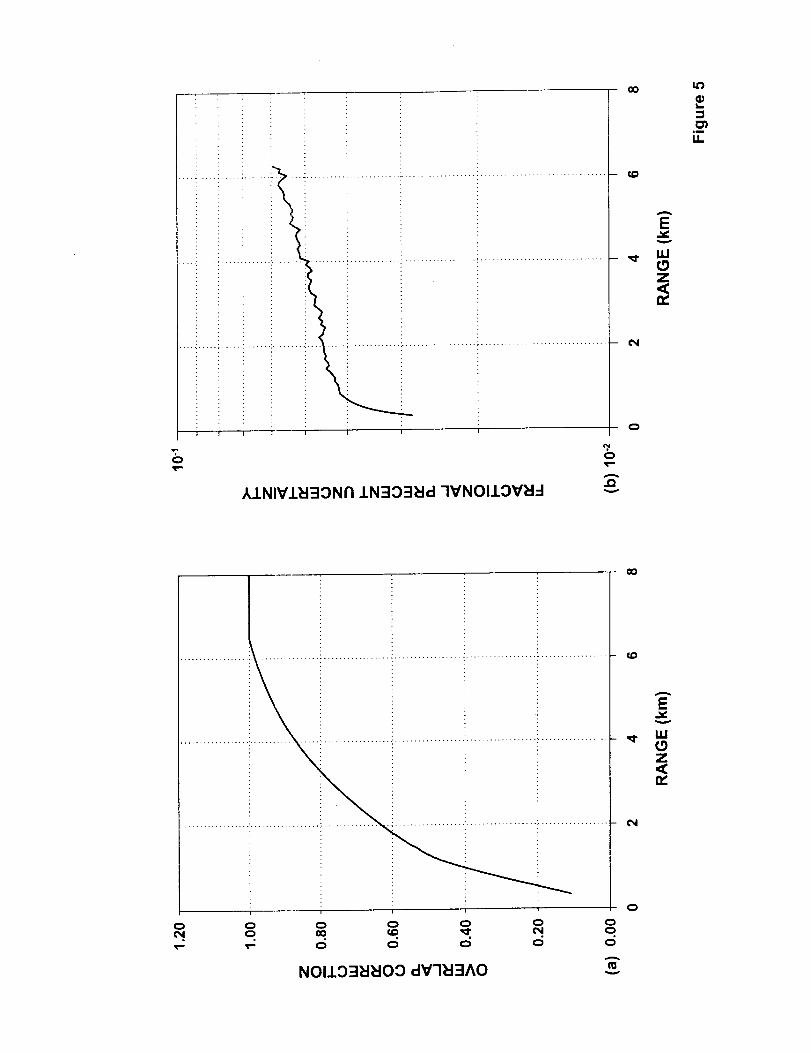
The final overlap uncertainty is calculated using Eq. (16). Figure 5 shows a typical overlap
function and its uncertainty.
Signals measured duling regular operations are overlap corrected by dividing PyA(r), Eq.
(11), by the pre-determined overlap, O(r). The resulting signal is termed the normalized-
afterpulse-overlap-corrected signal, PNAo(r), and is given by
P(r)-B-[EAN(r)]
P_AO(r) = E = PN_ (r_______) (25)O(r) r 2
13
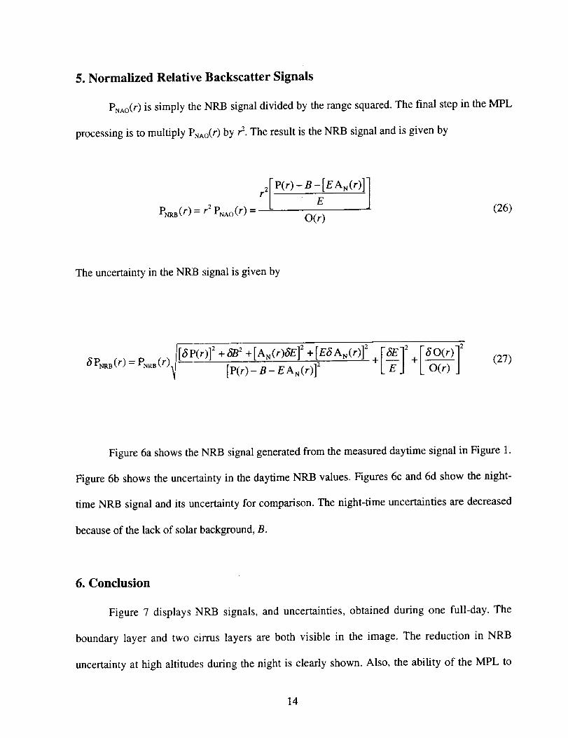
5. Normalized Relative Backscatter Signals
PNAO(r) is simply the NRB signal divided by the range squared. The final step in the MPL
processing is to multiply P_Ao(r) by rz. The result is the NRB signal and is given by
P_B(r) = r2 PNAo(r) =r2[ P(r)- B-[E AN(r)] ]-_
O(r)(26)
The uncertainty in the NRB ,_ignal is given by
(r)I[SP(r)]2+SB2 +[AN(r)_EI2+[EaAr_(r)] 2 2 +[SO(r)] 26P_s(r) = P_ [p(r)_B_EAN(r)] 2 _[-_] L O(r) j(27)
Figure 6a shows the NRB signal generated from the measured daytime signal in Figure 1.
Figure 6b shows the uncertainty in the daytime NRB values. Figures 6c and 6d show the night-
time NRB signal and its uncertainty for comparison. The night-time uncertainties are decreased
because of the lack of solar background, B.
6. Conclusion
Figure 7 displays NRB signals, and uncertainties, obtained during one full-day. The
boundary layer and two cirrus layers are both visible in the image. The reduction in NRB
uncertainty at high altitudes during the night is clearly shown. Also, the ability of the MPL to
14

detectthe presenceof moderateto thick cirrus layers at one-minutedatarate during mid-day
(low signal-to-noise)is shown.During mid-day, NRB signaluncertaintiesin clear air regions
approach100%at approximately6 km. However, whencirrus is encounteredthe NRB signal
uncertainties drop considerably due to an increase in the signal-to-noise within the cloud.
However, detecting thin cirrus during daytime at one-minute data rates is difficult. This problem
can be overcome by averaging NRB signals over several minute periods.
In general, near the surface, the overlap uncertainty is the dominant source of uncertainty
in the NRB signal. At altituctes above the overlap region, the dominant source of uncertainty in
the NRB signal is typically due to uncertainty in the energy. However, during daytime B
increases and reduces the signal-to-noise, which causes 6PNRB(r) to increase accordingly.
Therefore, during the daytime B is also a large source of uncertainty at higher altitudes.
15

Acknowledgements
This work was conducted by members of the MPL-Net project at NASA Goddard Space
Flight Center. The MPL-Net project is funded by the NASA Earth Observing System and the
SIMBIOS project. The authors thank Stan Scott, Tim Berkoff, Matt McGill, Dennis Hlavka, Bill
Hart, Jim Spinhirne, and Xiaoli Sun for helpful discussions on the matter of uncertainties in the
various MPL components.
16

References
Campbell, J. R., D. L. Hlavka, E. J. Welton, C. J. Flynn, D. D. Turner, J. D. Spinhirne, V. S.
Scott, and I. H. Hwang, 2001: Full-time, Eye-Safe Cloud and Aerosol Lidar Observation at
Atmospheric Radiation Measurement Program Sites: Instrument and Data Processing. J. Atmos.
Oceanic Technol., accepted.
Fernald, F. G., B. M. Herman, and J. A. Reagan, 1972: Determination of aerosol height
distributions by lidar, J. Appl. Meteorol., 11,482-489.
Peppier, R. A., C. P. Bahnnann, J. C. Barnard, J. R. Campbell, M. D. Cheng, R. A. Ferrare, R. N.
Halthore, L. A. Heilman, D. L. Hlavka, N. S. Laulainen, C. J. Lin, J. A. Ogren, M. R. Poellot, L.
A. Remer, K. Sassen, J. D. Spinhirne, M. E. Splitt, and D. D. Turner, 2000: ARM Southern
Great Plains Site Observations of the Smoke Pall Associated with the 1998 Central American
Fires. Bull. Amer. Meteor. Soc., 81, 2563-2591.
Sasano, Y., H. Shimizu, N. Takeuchi, and M. Okuda, 1979: Geometrical form factor in the laser
radar equation: an experimental determination. Appl. Opt., 18, 3908-3910.
Spinhirne, J. D., J. A. Reagan, and B. M. Herman, 1980: Vertical Distribution of Aerosol
Extinction Cross Section and Inference of Aerosol Imaginary Index in the Troposphere by Lidar
Technique. J. AppI. Meteoro/.., 19, 426-438.
Spinhime, J. D., 1993: Micro Pulse Lidar. IEEE Trans. Geosci. Remote Sens., 31, 48-55.
17

Spinhirne,J. D., J. A. R. Rail, and V. S.Scott, 1995:CompactEye SafeLidar Systems.Rev.
Laser Eng., 23, 112-118.
Stokes, G. M., and S. E. Schwartz, 1994: The Atmospheric Radiation Measurement (ARM)
Program: Programmatic background and design of the cloud and radiation testbed. Bull. Amer.
Meteorol. Soc., 75, 1201-1221.
Voss, K. J., E. J. Welton, P. K. Quinn, J. Johnson, A. Thompson, and H. Gordon, 2001: Lidar
Measurements During Aero,;ols99. J. Geophys. Res., 106, 20821-20832.
Welton, E. J., K. J. Voss, HI. R. Gordon, H. Maring, A. Smirnov, B. Holben, B. Schmid, J. M.
Livingston, P. B. Russell, P. A. Durkee, P. Formenti, M. O. Andreae, 2000: Ground-based Lidar
Measurements of Aerosols During ACE-2: Instrument Description, Results, and Comparisons
with other Ground-based and Airborne Measurements. Tellus B, 52, 635-650.
Welton, E. J., K. J. Voss, P. K. Quinn, P. J. Flatau, K. Markowicz, J. R. Campbell, J. D.
Spinhime, H. R. Gordon, and J. E. Johnson, 2001: Measurements of aerosol vertical profiles and
optical properties during h-NDOEX 1999 using micro-pulse lidars. J. Geophys. Res., in press.
18
Figure Captions
Figure 1. Example of MPL observed count rates (a). The uncertainty in the observed count rate
using Poisson statistics (b). Both day and night observations are shown.
Figure 2. The detector dead-time factor versus measured count rates (a). The fractional percent
uncertainty in the dead-time factor (b). The dead-time factor is only significant above 1.01, and
the uncertainties are below 0.3%.
Figure 3. Percent fluctuation in energy monitor values
temperature for the five different MPL systems in Table 1.
versus the percent fluctuation in
Figure 4. A typical normzdized afterpulse signal (a). The afterpulse percent uncertainty (b). The
afterpulse uncertainty is dominated by the uncertainty in the energy monitor value.
Figure 5. A typical overlap function (a) and its fractional percent uncertainty (b).
Figure 6. The results of coJrrections to the day and night MPL count rates from Figure 1 are
shown. The daytime NRB signal and uncertainty are shown in 6a and 6b, respectively. The
night-time NRB signal and uncertainty are shown in 6c and 6d, respectively.
Figure 7. NRB signals obtained during a full day of MPL observations are shown in the upper
panel. The bottom panel shows the NRB fractional percent uncertainty.
19

Table 1. Energy Uncertainty
MPL # Average % Fluctuation in Average % Fluctuation in
Energy (I.tJ) Energy Temperature (C °) Temperature
6.88 + 0.07 1.00 26.93 + 0.66 2.45
3.71 + 0.03 0.85 27.77 + 0.09 0.33
6.60 + 0.25 3.82 24.02 :t. 1.75 7.28
7.64 + 0.12 1.57 30.55 + 0.89 2.92
3.82 + 0.12 3.23 28.43 + 1.69 5.93
Samples (M)
318
1423
2823
1272
1204
2O

...................................................................... i.........
o
I.
U.
........................ i!......;................._....................................i ...............

ii i i i iii i i i i •
_,,<ii i i i i ! i iii ! i i i i o!
t_
: : : : : : : i i i ! ! i ! i i O i
i J , i ; ' --' _ I ' ' ' ' ' i , i I
AINIVI_I:IONn 1N:IO_l=Id 7VNOIlO_I_-I
rn
/ Ooo! ! i •
ii ii............................................:: ,........ _ _o°i i i •
i • oo_
:: i i • oo
........................... i i i_:.......................... :_........................... :_....................... °•• _ _
t,,,,,
I,,I.
A
_IOJ.OV::I NOI19:::I_I_IOO :II/II11cr¢3(] ----
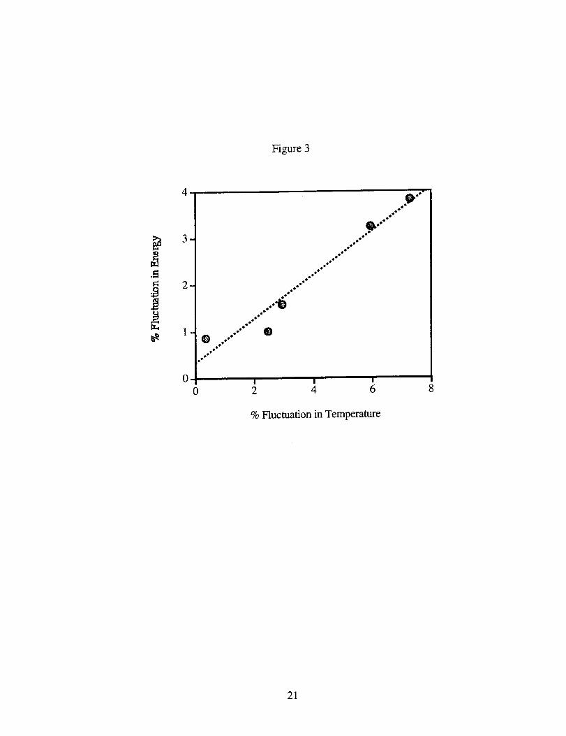
Figure 3
4
3_
2_
0
0I I I2 4 6 8
% Fluctuation in Temperature
21

o
..=,..,.......,,,: .... _ ...... | ......... ................. _..,...., .,..... .... ...... : ...... = ......... . ...............
i i i i i i i ! i ! i i i
i
o
AINIV.LId::IONI'I 1N::lO3_d -IVNOIJ.DV_Id
A
JO
(o
143
Ev
_ 0 111
Z
n,'
¢)
0"Iim
I.I.
J
0 0 0 0 0 0
I11
o
• 0o o Z
A
(_I) 39NVldUI ....,
NOIIO::I_I_IO0 dV-1_I3AO m

,.0
("'_1)30N_d
o
_z_
a,.
v
o
N
_ _ _ o
tO
t_°_
u.
AU
z_e-
(w_) 30N_rd
e-
ll.
,,.z
°o(W_l) 30 NV'_I
iz.l
l,,U
r_ _-U.l_,.__.v
0z

8 _q8<_
8
£
"E"O'
I
O
og_0" a=,.
'C-
ma
Q.
D .m
"D "3
Z
3(I-
>.-
J
@Or"
.=,
8
O
_8
mm
Zv
70
O
m&E
&
GSFC S]'I PUBLIC DISCLOSURE EXPORT CONTROL CHECKLIST
The Export Control Office requests your assistance in assuring that your proposed disclosure of NASA scientific and technical information (STI)
complies with the Export Administration Regulati,_ns (EAR, 15 CFR 730-774) and the International Traffic In Arms Regulations (ITAR, 22 CFR
120-130). The NASA Export Control Program requires that every domestic and international presentation/publication of GSFC STI be reviewed
through the GSFC Export Control Office in accordance with the NASA Form 1676 NASA Scientific and Technical Document Availability
Authorization (DAA) process. Release of NASA information into a public forum may provide countries with interests adverse to the United States
with access to NASA technology. Failure to c_mply with the ITAR regulations and/or the Commerce Department regulations may subject you to
fines of up to $1 million and/or up to ten years imprisonment per violation. Completion of this checklist should minimize delays in approving most
requests for presentation/publication of NASA ST1.
Generally, the export of information pertaining to the design, development, production, manufacture, assembly, operation, repair, testing,
maintenance or modification of defense articles, i.e., space flight hardware, ground tracking systems, launch vehicles to include sounding rockets and
meteorological rockets, radiation hardened hardware and associated hardware and engineering units for these items are controlled by the State
Department under the ITAR. A complete listing of items covered by the ITAR can be accessed at http://gsfc-blucnun.gsfc.nasa.
gov/export/regsitar.htm. The export of information with respect to ground based sensors, detectors, high-speed computers, and national security and
missile technology items are controlled by the U.S. Commerce Department under the EAR. If the information intended for release falls within the
above categories but otherwise fits into one or more of the following exemptions, the information may be released.
EXEMPTION I
If your information is already in the public domain in it's entirety through a non-NASA medium and/or through NASA release previously approved
by the Export Control Office, the information is e:_empt from further review. If the information falls into this category, you may attest that you are
using this exemption by signing below.
Signature Date
EXEMPTION !!
If your information pertains exclusively to the release of scientific data, i.e. data pertaining to studies of clouds, soil, vegetation, oceans, and planets,
without the disclosure of information pertaining to articles controlled by the ITAR or EAR, such as flight instruments, high speed computers, or
launch vehicles, the information is exempt from filrther review. If the information falls into this category, you may attest that you are using this
exemption by signing below.
, i2.- '-01Signatur Date
EXEMPTION I!I
If your information falls into the areas of concern as referenced above, but is offered at a general purpose or high level, i.e. poster briefs and
overviews, where no specific information pe_ining to ITAR or EAR controlled items is offered, the information is exempt from further review. If
the information falls into this category, you may attest that you are using this exemption by signing below.
Signature Date
EXEMPTION IV
If your information is not satisfied by the 3 exemptions stated above, the information may be released using exemption 125.4(bX13) of the ITAR.
Use of this exemption is afforded only to agencie,; of the Federal Government and allows the release of ITAR controlled information into the public
domain. But the GSFC Export Control Office has determined that use of this exemption will be allowed only after we receive assurance that such
release is a responsible action. To this end, an internal guideline has been established pursuant to the use of this exemption: That the information
does not offer specific insight into design, design methodology, or design processes of an identified ITAR controlled item in sufficient detail (by
itself or in conjunction with other publications) to allow a potential adversary to replicate, exploit and/or defeat controlled U.S. technologies. All
signatures of approval on NASA Form 1676 e_prcssly indicate concurrence with the responsible use of Exemption IV when Exemption IV has been
cited by the author. If you determine that you have met this criteria, you may attest your determination by signing below, and the GSFC Export
Control Office will offer favorable consideration l:oward approving your presentation/publication request under this special exemption.
Signature l)ate
If you do not satisfy the above exemptions, please contact the GSFC Export Control Office for further clarification on the releasability of your
information under the ITAR or EAR.
1/8/1999


