ARTICLE IN PRESS
0038-0717/$ - se
doi:10.1016/j.so
�CorrespondE-mail addr
(M. Zimmerma
Soil Biology & Biochemistry 39 (2007) 224–231
www.elsevier.com/locate/soilbio
Quantifying soil organic carbon fractions by infrared-spectroscopy
M. Zimmermann�, J. Leifeld, J. Fuhrer
Agroscope ART Reckenholz, Swiss Federal Research Station for Agroecology and Agriculture, Air Pollution/Climate Group, Reckenholzstrasse 191,
8046 Zurich, Switzerland
Received 20 April 2006; received in revised form 26 June 2006; accepted 21 July 2006
Available online 31 August 2006
Abstract
Methods to quantify organic carbon (OC) in soil fractions of different stabilities often involve time-consuming physical and chemical
treatments. The aim of the present study was to test a more rapid alternative, which is based on the spectroscopic analysis of bulk soils in
the mid-infrared region (4000–400 cm�1), combined with partial least-squares regression (PLS). One hundred eleven soil samples from
arable and grassland sites across Switzerland were separated into fractions of dissolved OC, particulate organic matter (POM), sand and
stable aggregates, silt and clay particles, and oxidation resistant OC. Measured contents of OC in each fraction were then correlated by
PLS with infrared spectra to obtain prediction models. For every prediction model, 100 soil spectra were used in the PLS calibration and
the residual 11 spectra for validation of the models. Correlation coefficients (r) between measured and PLS-predicted values ranged
between 0.89 and 0.97 for OC in different fractions. By combining different fractions to one labile, one stabilized and one resistant
fraction, predictions could even be improved (r ¼ 0:98, standard error of prediction ¼ 16%). Based on these statistical parameters, we
conclude that mid-infrared spectroscopy in combination with PLS is an appropriate and very fast tool to quantify OC contents in
different soil fractions.
r 2006 Elsevier Ltd. All rights reserved.
Keywords: Carbon fractions; Mid-infrared spectroscopy; Partial least-squares regression
1. Introduction
Organic carbon (OC) in agricultural soils is of increasinginterest. This is not only because of its well-knownbeneficial effect on nutrient dynamics and soil structure,but also because of its potential role as a sink foratmospheric carbon dioxide (CO2) (IPCC, 2000). Changesin the type and intensity of land management, or in landuse such as conversion of cropland to grassland, canpositively influence the sequestration of atmosphericcarbon (Lal, 2004; DeGryze et al., 2004), and thus couldpotentially play an important role in the mitigation ofclimate change.
Both land-use and soil management influence theamount of OC in soils in many ways, positively as well asnegatively. But these influences are not of equal concern toall parts of the soil system. Importantly, they differ
e front matter r 2006 Elsevier Ltd. All rights reserved.
ilbio.2006.07.010
ing author. Tel.: +4144 377 7125; fax: +41 44 377 7201.
ess: [email protected]
nn).
between soil fractions of different physical and chemicalstabilities. Soil samples can be separated into fractions thatare either (i) easily decomposable, (ii) stabilized byphysical–chemical mechanisms or (iii) biochemically recal-citrant. Fresh plant residues are only partly incorporatedinto the soil matrix. Thus, they are easily available formicroorganisms and, consequently, rapidly decomposed.By further incorporation into the soil matrix, OC becomesstabilized either through physical protection inside aggre-gates, where access by microorganisms is restricted, orphysico-chemically by binding onto mineral surfaces of siltand clay particles (Six et al., 2002a). Biomolecules ofdegraded SOM are even biochemically recalcitrant (Krulland Skjemstad, 2003).Various methods have been proposed to separate soil
samples into fractions with distinct chemical and physicalcharacteristics corresponding to different stabilizing me-chanisms and soil functions. Typically, these methods wereused to determine the OC content of the different soilfractions in order to calculate turnover times, and toidentify relationships between the distribution of OC
ARTICLE IN PRESSM. Zimmermann et al. / Soil Biology & Biochemistry 39 (2007) 224–231 225
between the different fractions and soil management orland-use (Hassink et al., 1997; Sohi et al., 2001; Six et al.,2002b; John et al., 2005). Most of the proposed proceduresincluded dispersion of aggregates and isolation of a lightparticulate organic matter (POM) fraction. This latterfraction has been shown to play a crucial role in theformation of aggregates (Six et al., 2001), and to be mostsensitive to changes in soil management (Franzluebbersand Stuedemann, 2002). To obtain a chemically resistantfraction, treatments like hydrolysis or oxidation are appliedto plant-free soil fractions (Paul et al., 1997; Siregar et al.,2005). These fractionation procedures have in commonthat they are very time-consuming. For routine investiga-tions, more rapid methods are needed.
A combination of spectroscopic measurement andpartial least-squares regression (PLS) was introduced byHaaland and Thomas (1988) to quantify different chemicalcompounds. PLS is a chemometric method to deriveprediction models for specific compounds from spectro-scopic data. Later, Janik and Skjemstad (1995) quantifieddifferent properties of bulk soils by combining PLS withmid-infrared spectra. Since then, PLS was applied invarious studies to estimate bulk soil characteristics fromvisible, near- and mid-infrared spectroscopic measurements(Viscarra-Rossel et al., 2006). Most recently, Cozzolinoand Moron (2006) quantified OC of particle-size fractionsby near-infrared spectroscopy and PLS, thus indicating thepotential of this approach for rapid analysis of OC in soilsize-fractions.
In the present study, we aimed to go one step further.The objective was to quantify OC from differentlystabilized soil fractions by use of mid-infrared spectraobtained from bulk samples of agricultural topsoils. Theapproach was to first fractionate the samples by acombination of different treatments to obtain two labile,two stabilized and one chemically resistant fraction, andthen to determine the amounts of OC in these fractions andto correlate OC contents with data obtained from infraredspectra of bulk soil samples using PLS. Finally, thesecorrelations were used as a set of predictive models, whichcould be tested using independent data from OC measure-ments.
2. Materials and methods
2.1. Soil samples
We fractionated 111 archived soil samples from twodifferent research projects in Switzerland. One archive wasthe collection of the Swiss national soil survey, from whichwe analysed 41 samples representing agriculturally mana-ged (arable land, temperate and alpine permanent grass-land) sites across Switzerland. Sampling sites varied inaltitudes from 265 to 2400m above sea level (a.s.l.)representing a gradient in mean annual temperaturebetween +10.6 and �1.6 1C, and in mean annualprecipitation from 722 to 2327mm. Undisturbed grassland
soils were divided into horizons of 0–5 cm, 5–10 cm,10–20 cm, 0–10 cm or 0–20 cm. Disturbed soils from arablesites were taken as one horizon from 0 to 20 cm. A detaileddescription of the sampling technique, together with sitecharacteristics such as soil properties, climate, geology andland-use, are given in Desaules and Studer (1993).A second set with 70 soil samples were obtained from a
biodiversity study in temperate grasslands on the SwissCentral Plateau. These samples originated from threedifferent regions at altitudes between 420 and 670m a.s.l.with an annual precipitation between 964 and 1333mm.Each soil sample was a composite of 20 soil cores takenfrom the top 20 cm. Management intensities of thesegrassland sites varied considerably, as described in detailby Buholzer et al. (2005).Since soil samples included in a PLS prediction model
should have similar spectral properties, only carbonate-freesoils with an organic matter (OM) content of less than 15%were used. Both, carbonate and OM cause distinct peaks ininfrared spectra, which may interfere with other peaks.Bulk soil samples were dried at 40 1C, crushed, andparticles 42mm were removed. Silt and clay contentswere determined by the pipette method and sand contentcalculated by difference (FAC, 1989). Carbon and nitrogencontents of all archived bulk soil samples were measurednewly before fractionating the soil samples after drycombustion with an elemental analyzer (Vario EL,Elementar).
2.2. Fractionation procedure
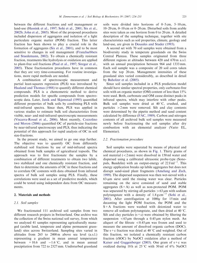
Soil samples were separated by means of physical andchemical procedures, as shown in Fig. 1. Thirty grams ofsoil material (o2mm) were dissolved in 150ml water anddispersed using a calibrated ultrasonic probe-type (Sono-puls, Bandelin) with an output-energy of 22 Jml�1. Thisenergy application breaks up labile aggregates but does notdisrupt sand-sized plant fragments (Amelung and Zech,1999). The dispersed suspension was then wet-sieved with a63-mm sieve until the rinsing water was clear. Particlesremaining on the sieve consisted of sand and stableaggregates (S+A) as well as non-protected POM. POMwas separated by stirring all particles 463 mm with sodiumpolytungstate with a density of 1.8 g cm�3 (Sohi et al.,2001). After centrifugation at 1000g for 15min anddecanting the light POM fraction, the POM and theS+A fractions were washed with deionized water toremove all sodium polytungstate, and then dried at 40 1C.Silt and clay particles (s+c) were obtained by filtering thesuspension o63 mm through a 0.45 mm nylon mesh. Analiquot of the filtrate o0.45 mm was frozen and used tomeasure the amount of dissolved organic carbon (DOC).The s+c fraction was dried at 40 1C and weighted. Out ofthis fraction, we isolated a chemically resistant carbonfraction (rSOC) by NaOCl oxidation after a method ofKaiser and Guggenberger (2003). One gram of s+c wasoxidized during 18 h at 25 1C with 50ml of 6% NaOCl
ARTICLE IN PRESS
rSOC
POM
s+c
S+A
DOC
bulk soil < 2 mmdispersion
with 22 J ml-1,wet sievingto 63 µm
fraction < 63 µm
suspension< 0.45 µm
fraction > 63 µm, afterwards density-
separationat 1.8 g cm-3
heavyfraction
lightfraction
soil fractions carbon fractions
NaOClresistantfraction
s+c-rSOC
labilefraction
resistantfraction
stabilizedfraction
Fig. 1. Procedure to obtain the following organic carbon fractions: dissolved organic carbon (DOC), particulate organic matter (POM), sand and stable
aggregates (S+A), silt and clay particles (s+c), and oxidation-resistant carbon (rSOC). Adding POM+DOC yields a combined labile fraction, and
S+A+(s+c�rSOC) a combined stabilized fraction.
M. Zimmermann et al. / Soil Biology & Biochemistry 39 (2007) 224–231226
(wt/wt) adjusted to pH 8 with concentrated HCl. Residueswere centrifuged at 1000g for 15min, decanted, washedwith deionized water, and then centrifuged again. Thisoxidation step was repeated twice. Carbon and nitrogencontents in all solid fractions were measured by combus-tion with an elemental analyzer (Vario EL, Elementar), andin liquid samples by thermal oxidation with a liquidanalyser (Dimatoc 2000, Dimatec).
With reference to the stabilizing mechanisms describedabove, OC contents of the fractions DOC and POM werecombined to yield one labile fraction, and OC contents ofS+A and s+c minus rSOC were combined to obtain onestabilized fraction.
2.3. DRIFT spectroscopy
Infrared spectra were recorded in reflectance mode witha Perkin Elmer Spectrum One spectrometer with DiffuseReflectance Infrared Fourier Transformation (DRIFT)inlet. Bulk soil samples were diluted with 97% KBr toreduce scatter light intensity, homogenized for 30 s in a ballmill, and then scanned 16 times in the range from 4000 to400 cm�1 (mid-infrared region) with a resolution of 4 cm�1.KBr background spectra were subtracted from themeasured spectra. DRIFT spectra were corrected againstatmospheric CO2 and water vapour and automaticallyadjusted to an internal CH4 cell. In the following, infraredregions are ascribed to functional groups according to Baesand Bloom (1989).
2.4. PLS quantification
For PLS, spectral information is arranged as n�m
matrix which consists of n spectra with absorbance valuesfor m wavelengths, and the calibration data is expressed asa single vector with the measured values for these spectra(Kramer, 1998). The PLS1 algorithm decomposes the m-dimensional spectra space into few factors termed latentvariables (LV), which represent the best projections of thecalibration vector onto the n�m matrix. One of theadvantages of PLS compared to other chemometricmethods like principal component analysis is the possibilityto interpret the first few LV, because they show thecorrelations between the property values and the spectralfeatures (Kramer, 1998). Furthermore, PLS takes as wellvariations of the absorbance as variations of the calibrationdata into account. A separate prediction model has to beevaluated for every compound that will be estimated byPLS. The exact decomposition process conducted by thePLS1 algorithm is described in detail in Martens and Naes(1989).We divided all DRIFT spectra for each PLS prediction
model into two separate sets for calibration and validation.All soil samples (n ¼ 111) were arranged for each caseaccording to measured property values (i.e. clay content,total OC and nitrogen, or amount of OC in the differentfractions). The DRIFT spectra of every 10th soil sample,beginning with number 5, was allocated to the validationsubset (n ¼ 11). Individual prediction models for every
ARTICLE IN PRESS
6 10 12 14 16 18
number of LV
2.0
2.5
3.0
3.5
4.0
4.5
5.0
SE
P (
)
1.00
1.02
1.04
1.06
1.08
1.10
slop
e (
)
best fit with 12 LV
y = 1.021x
SEP = 2.79
8
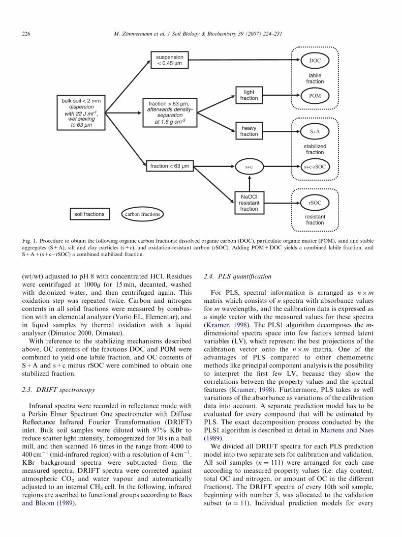
Fig. 2. Determination of the optimal number of latent variables (LV):
relationship between number of number LV and standard error of
prediction (SEP) (m) and slope of regression equation through zero (J)
for measured vs. PLS-predicted data for total organic carbon.
M. Zimmermann et al. / Soil Biology & Biochemistry 39 (2007) 224–231 227
property were then computed with the software SpectrumQuant+ (Perkin Elmer, Version 4.51.02) using the datafrom the 100 calibration spectra. Spectra were importedinto the software in absorbance units and scaled to a meanof zero. The data range was reduced to between 4000 and600 cm�1 in order to remove signal noise in the regionbetween 600 and 400 cm�1. The software was forced todecompose the spectra matrix into 30 LV, and to validatethis decomposition process internally by full cross-valida-tion. During full cross-validation, each spectrum was inturn excluded from the calibration sample set and waspredicted by the PLS model calculated with the remainingspectra. To detect outliers, leverage values were consulted,which can be conceived as the distance between a singlespectrum and the centre of the entire data matrix. Spectrawith leverage values higher than twice the mean leveragevalue of all spectra were excluded from the calibration. Bydecomposing the spectra into 30 LV, it was assumed thatthe prediction model would be over-fitted because signalnoise of the spectral measurements could also be correlatedwith the property vector (Martens and Naes, 1989). Theoptimal numbers of LV were found by testing 1–30 LV inthe prediction model and comparing the predicted valuesof each PLS model with the measured ones. For this, theprediction models calibrated on 100 DRIFT spectra wereapplied to the 11 DRIFT spectra of the validation set, andthe PLS predicted and the laboratorial quantified valuescompared. To decide which prediction model fitted best,standard errors of prediction (SEP) and slopes of theregression equations through the origin between predictedand measured values for 1–30 LV were compared.Standard error of prediction (SEP) values were calculatedas
SEP ¼
ffiffiffiffiffiffiffiffiffiffiffiffiffiffiffiffiffiffiffiffiffiffiffiffiffiffiffiPðxm � xpÞ
2
n� 1
s, (1)
where xm are measured values, xp PLS-predicted values,and n is the number of samples used for validation. Theprediction model with the lowest SEP and a slope closest to1 was considered as best fit (Fig. 2). To compare SEPvalues of prediction models for different data ranges,relative SEP (rel SEP) was calculated as
rel SEP ¼SEP
x� 100 (2)
with x as the mean of the validation data range. Theappropriateness of a chemometric prediction method wasevaluated by the residual prediction deviation (RPD),which is the ratio between the standard deviation (s.d.) ofthe validation sample set and the SEP (Willimas andNorris, 1987):
RPD ¼s:d:
SEP. (3)
In agricultural applications, RPD values 43 areconsidered satisfactory, whereas prediction models with
RPD values o3 should only be used as screening methods(Malley et al., 2000).
3. Results and discussion
3.1. Carbon distribution among fractions
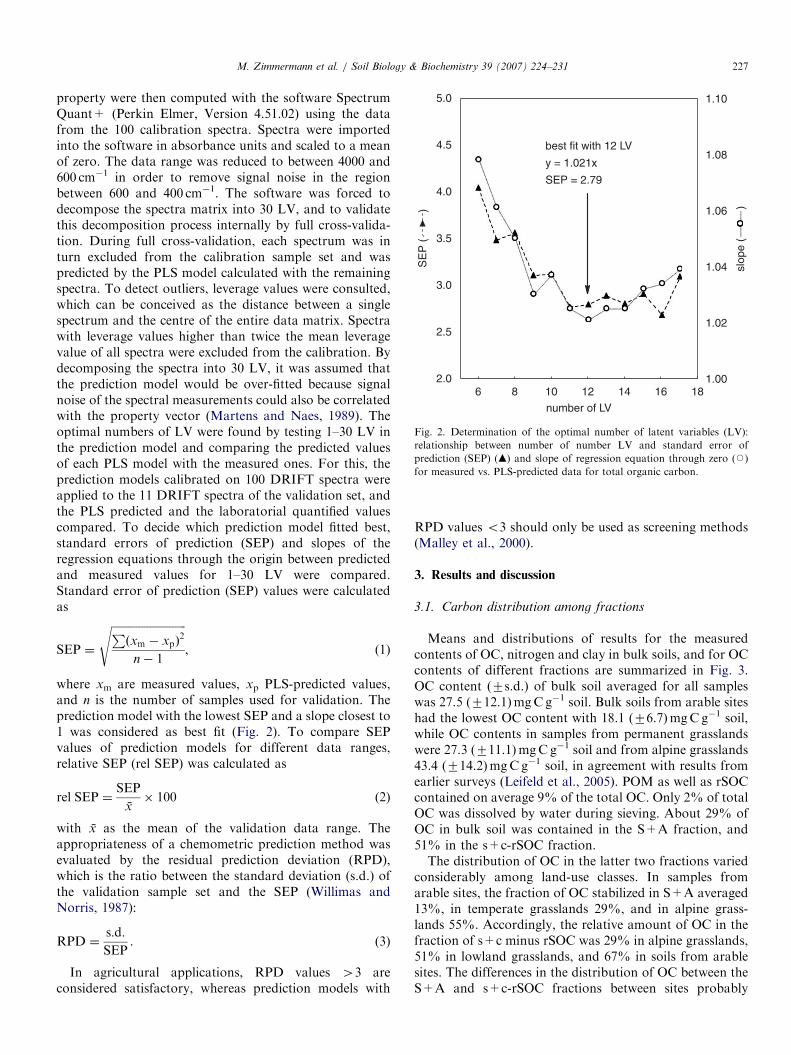
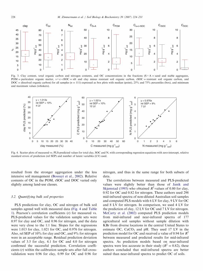
Means and distributions of results for the measuredcontents of OC, nitrogen and clay in bulk soils, and for OCcontents of different fractions are summarized in Fig. 3.OC content (7s.d.) of bulk soil averaged for all sampleswas 27.5 (712.1)mgCg�1 soil. Bulk soils from arable siteshad the lowest OC content with 18.1 (76.7)mgCg�1 soil,while OC contents in samples from permanent grasslandswere 27.3 (711.1)mgCg�1 soil and from alpine grasslands43.4 (714.2)mgCg�1 soil, in agreement with results fromearlier surveys (Leifeld et al., 2005). POM as well as rSOCcontained on average 9% of the total OC. Only 2% of totalOC was dissolved by water during sieving. About 29% ofOC in bulk soil was contained in the S+A fraction, and51% in the s+c-rSOC fraction.The distribution of OC in the latter two fractions varied
considerably among land-use classes. In samples fromarable sites, the fraction of OC stabilized in S+A averaged13%, in temperate grasslands 29%, and in alpine grass-lands 55%. Accordingly, the relative amount of OC in thefraction of s+c minus rSOC was 29% in alpine grasslands,51% in lowland grasslands, and 67% in soils from arablesites. The differences in the distribution of OC between theS+A and s+c-rSOC fractions between sites probably
ARTICLE IN PRESS
Ctot CS+A CPOM CrSOCCs+c-rSOCclay Ntot
0
10
20
30
40
50
60
70
80
0
1
2
3
4
5
6
7
8
0
5
10
15
20
25
30
35
40
45
CDOC
mg
g-1so
il
mg
g-1so
il
mg
g-1so
il
mg
g-1so
il
mg
g-1so
il
mg
g-1so
il
mg
g-1so
il
%
0
2
4
6
8
10
0
10
20
30
40
50
0
5
10
15
20
25
30
0
2
4
6
8
10
0
2
4
6
8
10
Fig. 3. Clay content, total organic carbon and nitrogen contents, and OC concentrations in the fractions (S+A ¼ sand and stable aggregates,
POM ¼ particulate organic matter, s+c�rSOC ¼ silt and clay minus resistant soil organic carbon, rSOC ¼ resistant soil organic carbon, and
DOC ¼ dissolved organic carbon) for all samples (n ¼ 111) expressed as box plots with median (point), 25% and 75% percentiles (box), and minimum
and maximum values (whiskers).
0
C measured (mg g-1soil)
0
10
10
20
20
30
30
40
40
50
50
60
60
C P
LS p
redi
cted
(m
g g-1
soil)
0 5 10 15 20 25 30 35 40
clay measured (%)
0
5
10
15
20
25
30
35
40
clay
PLS
pre
dict
ed (
%)
0 1 2 3 4 5 6
N measured (mg g-1soil)
0
1
2
3
4
5
6
N P
LS p
redi
cted
(m
g g-1
soil)
y = 1.013xrel SEP = 10%4 LV
y = 1.021xrel SEP = 10%12 LV
y = 0.976xrel SEP = 9%7 LV
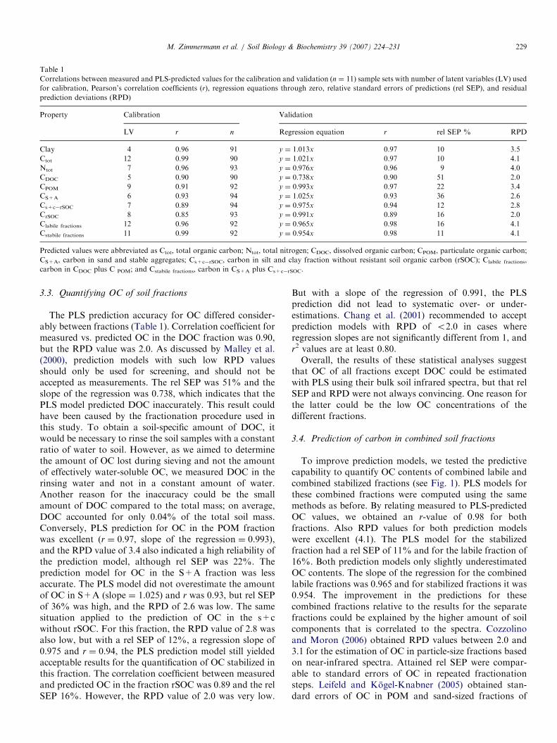
Fig. 4. Scatter plots of measured vs. PLS-predicted values for total clay, SOC and N, with corresponding regression equations with zero-intercept, relative
standard errors of prediction (rel SEP) and number of latent variables (LV) used.
M. Zimmermann et al. / Soil Biology & Biochemistry 39 (2007) 224–231228
resulted from the stronger aggregation under the lessintensive soil management (Bossuyt et al., 2002). Relativecontents of OC in the POM, rSOC and DOC varied onlyslightly among land-use classes.
3.2. Quantifying bulk soil properties
PLS predictions for clay, OC and nitrogen of bulk soilsamples agreed well with measured data (Fig. 4 and Table1). Pearson’s correlation coefficients (r) for measured vs.PLS-predicted values for the validation sample sets were0.97 for clay and OC, and 0.96 for nitrogen, and the datawere very close to the 1:1 line. Slopes for the regressionswere 1.013 for clay, 1.021 for OC, and 0.976 for nitrogen.Also, rel SEP of 10% for clay and OC, and 9% for nitrogenwere in an acceptable range. Residual prediction deviationvalues of 3.5 for clay, 4.1 for OC and 4.0 for nitrogenconfirmed the successful prediction. Correlation coeffi-cients (r) within the calibration sample sets after full cross-validation were 0.96 for clay, 0.99 for OC and 0.96 for
nitrogen, and thus in the same range for both subsets ofdata.The correlations between measured and PLS-predicted
values were slightly better than those of Janik andSkjemstad (1995) who obtained R2-values of 0.80 for clay,0.92 for OC and 0.82 for nitrogen. These authors used 298mid-infrared spectra of non-diluted Australian soil samplesand computed PLS models with 6 LV for clay, 9 LV for OCand 8 LV for nitrogen. In comparison, we used 4 LV forthe prediction of clay, 12 LV for OC and 7 LV for nitrogen.McCarty et al. (2002) computed PLS prediction modelsfrom mid-infrared and near-infrared spectra of 177agricultural soil samples without sample dilution withKBr from diverse locations in the central United States toestimate OC, CaCO3 and pH. They used 17 LV in theprediction model for OC and received a value of 0.94 for R2
between measured and predicted results for mid-infraredspectra. As prediction models based on near-infraredspectra were less accurate in their study (R2 ¼ 0:82), theseauthors concluded that mid-infrared spectra are bettersuited than near-infrared spectra to predict OC of soils.
ARTICLE IN PRESS
Table 1
Correlations between measured and PLS-predicted values for the calibration and validation (n ¼ 11) sample sets with number of latent variables (LV) used
for calibration, Pearson’s correlation coefficients (r), regression equations through zero, relative standard errors of predictions (rel SEP), and residual
prediction deviations (RPD)
Property Calibration Validation
LV r n Regression equation r rel SEP % RPD
Clay 4 0.96 91 y ¼ 1:013x 0.97 10 3.5
Ctot 12 0.99 90 y ¼ 1:021x 0.97 10 4.1
Ntot 7 0.96 93 y ¼ 0:976x 0.96 9 4.0
CDOC 5 0.90 90 y ¼ 0:738x 0.90 51 2.0
CPOM 9 0.91 92 y ¼ 0:993x 0.97 22 3.4
CS+A 6 0.93 94 y ¼ 1:025x 0.93 36 2.6
Cs+c�rSOC 7 0.89 94 y ¼ 0:975x 0.94 12 2.8
CrSOC 8 0.85 93 y ¼ 0:991x 0.89 16 2.0
Clabile fractions 12 0.96 92 y ¼ 0:965x 0.98 16 4.1
Cstabile fractions 11 0.99 92 y ¼ 0:954x 0.98 11 4.1
Predicted values were abbreviated as Ctot, total organic carbon; Ntot, total nitrogen; CDOC, dissolved organic carbon; CPOM, particulate organic carbon;
CS+A, carbon in sand and stable aggregates; Cs+c�rSOC, carbon in silt and clay fraction without resistant soil organic carbon (rSOC); Clabile fractions,
carbon in CDOC plus C POM; and Cstabile fractions, carbon in CS+A plus Cs+c�rSOC.
M. Zimmermann et al. / Soil Biology & Biochemistry 39 (2007) 224–231 229
3.3. Quantifying OC of soil fractions
The PLS prediction accuracy for OC differed consider-ably between fractions (Table 1). Correlation coefficient formeasured vs. predicted OC in the DOC fraction was 0.90,but the RPD value was 2.0. As discussed by Malley et al.(2000), prediction models with such low RPD valuesshould only be used for screening, and should not beaccepted as measurements. The rel SEP was 51% and theslope of the regression was 0.738, which indicates that thePLS model predicted DOC inaccurately. This result couldhave been caused by the fractionation procedure used inthis study. To obtain a soil-specific amount of DOC, itwould be necessary to rinse the soil samples with a constantratio of water to soil. However, as we aimed to determinethe amount of OC lost during sieving and not the amountof effectively water-soluble OC, we measured DOC in therinsing water and not in a constant amount of water.Another reason for the inaccuracy could be the smallamount of DOC compared to the total mass; on average,DOC accounted for only 0.04% of the total soil mass.Conversely, PLS prediction for OC in the POM fractionwas excellent (r ¼ 0.97, slope of the regression ¼ 0.993),and the RPD value of 3.4 also indicated a high reliability ofthe prediction model, although rel SEP was 22%. Theprediction model for OC in the S+A fraction was lessaccurate. The PLS model did not overestimate the amountof OC in S+A (slope ¼ 1.025) and r was 0.93, but rel SEPof 36% was high, and the RPD of 2.6 was low. The samesituation applied to the prediction of OC in the s+cwithout rSOC. For this fraction, the RPD value of 2.8 wasalso low, but with a rel SEP of 12%, a regression slope of0.975 and r ¼ 0.94, the PLS prediction model still yieldedacceptable results for the quantification of OC stabilized inthis fraction. The correlation coefficient between measuredand predicted OC in the fraction rSOC was 0.89 and the relSEP 16%. However, the RPD value of 2.0 was very low.
But with a slope of the regression of 0.991, the PLSprediction did not lead to systematic over- or under-estimations. Chang et al. (2001) recommended to acceptprediction models with RPD of o2.0 in cases whereregression slopes are not significantly different from 1, andr2 values are at least 0.80.Overall, the results of these statistical analyses suggest
that OC of all fractions except DOC could be estimatedwith PLS using their bulk soil infrared spectra, but that relSEP and RPD were not always convincing. One reason forthe latter could be the low OC concentrations of thedifferent fractions.
3.4. Prediction of carbon in combined soil fractions
To improve prediction models, we tested the predictivecapability to quantify OC contents of combined labile andcombined stabilized fractions (see Fig. 1). PLS models forthese combined fractions were computed using the samemethods as before. By relating measured to PLS-predictedOC values, we obtained an r-value of 0.98 for bothfractions. Also RPD values for both prediction modelswere excellent (4.1). The PLS model for the stabilizedfraction had a rel SEP of 11% and for the labile fraction of16%. Both prediction models only slightly underestimatedOC contents. The slope of the regression for the combinedlabile fractions was 0.965 and for stabilized fractions it was0.954. The improvement in the predictions for thesecombined fractions relative to the results for the separatefractions could be explained by the higher amount of soilcomponents that is correlated to the spectra. Cozzolinoand Moron (2006) obtained RPD values between 2.0 and3.1 for the estimation of OC in particle-size fractions basedon near-infrared spectra. Attained rel SEP were compar-able to standard errors of OC in repeated fractionationsteps. Leifeld and Kogel-Knabner (2005) obtained stan-dard errors of OC in POM and sand-sized fractions of
ARTICLE IN PRESS
labile OC resistant OCstabilized OC
4000 2000 1000 600
cm-1
4000 2000 1000 600
cm-1
4000 2000 1000 600
cm-1
(i)
(ii)
(iii)
(iv)
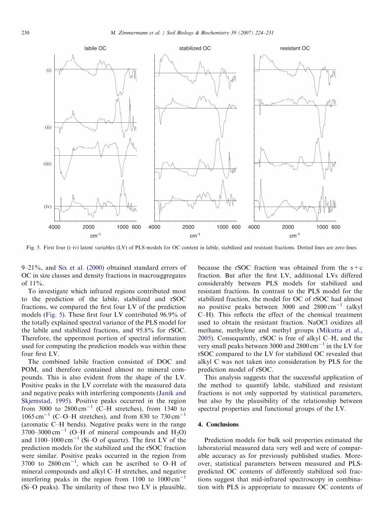
Fig. 5. First four (i–iv) latent variables (LV) of PLS models for OC content in labile, stabilized and resistant fractions. Dotted lines are zero lines.
M. Zimmermann et al. / Soil Biology & Biochemistry 39 (2007) 224–231230
9–21%, and Six et al. (2000) obtained standard errors ofOC in size classes and density fractions in macroaggregatesof 11%.
To investigate which infrared regions contributed mostto the prediction of the labile, stabilized and rSOCfractions, we compared the first four LV of the predictionmodels (Fig. 5). These first four LV contributed 96.9% ofthe totally explained spectral variance of the PLS model forthe labile and stabilized fractions, and 95.8% for rSOC.Therefore, the uppermost portion of spectral informationused for computing the prediction models was within thesefour first LV.
The combined labile fraction consisted of DOC andPOM, and therefore contained almost no mineral com-pounds. This is also evident from the shape of the LV.Positive peaks in the LV correlate with the measured dataand negative peaks with interfering components (Janik andSkjemstad, 1995). Positive peaks occurred in the regionfrom 3000 to 2800 cm�1 (C–H stretches), from 1340 to1065 cm�1 (C–O–H stretches), and from 830 to 730 cm�1
(aromatic C–H bends). Negative peaks were in the range3700–3000 cm�1 (O–H of mineral compounds and H2O)and 1100–1000 cm�1 (Si–O of quartz). The first LV of theprediction models for the stabilized and the rSOC fractionwere similar. Positive peaks occurred in the region from3700 to 2800 cm�1, which can be ascribed to O–H ofmineral compounds and alkyl C–H stretches, and negativeinterfering peaks in the region from 1100 to 1000 cm�1
(Si–O peaks). The similarity of these two LV is plausible,
because the rSOC fraction was obtained from the s+cfraction. But after the first LV, additional LVs differedconsiderably between PLS models for stabilized andresistant fractions. In contrast to the PLS model for thestabilized fraction, the model for OC of rSOC had almostno positive peaks between 3000 and 2800 cm�1 (alkylC–H). This reflects the effect of the chemical treatmentused to obtain the resistant fraction. NaOCl oxidizes allmethane, methylene and methyl groups (Mikutta et al.,2005). Consequently, rSOC is free of alkyl C–H, and thevery small peaks between 3000 and 2800 cm�1 in the LV forrSOC compared to the LV for stabilized OC revealed thatalkyl C was not taken into consideration by PLS for theprediction model of rSOC.This analysis suggests that the successful application of
the method to quantify labile, stabilized and resistantfractions is not only supported by statistical parameters,but also by the plausibility of the relationship betweenspectral properties and functional groups of the LV.
4. Conclusions
Prediction models for bulk soil properties estimated thelaboratorial measured data very well and were of compar-able accuracy as for previously published studies. More-over, statistical parameters between measured and PLS-predicted OC contents of differently stabilized soil frac-tions suggest that mid-infrared spectroscopy in combina-tion with PLS is appropriate to measure OC contents of
ARTICLE IN PRESSM. Zimmermann et al. / Soil Biology & Biochemistry 39 (2007) 224–231 231
labile, stabilized and resistant OC fractions out of bulk soilspectra. Infrared regions considered by PLS to compute theprediction models emphasize the reasonable relationshipbetween spectral properties and functional OC groups ofthe fractions. Furthermore, the quantification of soilcarbon fractions from bulk soil DRIFT spectra, whichtakes just some minutes, is much faster than fractionatingsoil samples by chemical and physical methods andmeasuring the carbon contents of the fractions afterwards.Thus, the proposed method can be very helpful inanalyzing large numbers of samples for effects of agricul-tural management and land-use or land-use changes ontotal OC content, and on differently stabilized OCfractions.
Acknowledgements
This study was financed by the Swiss Federal Office forthe Environment. We thank the Swiss National Soil Survey(NABO) and H.-R. Oberholzer for providing the soilsamples.
References
Amelung, W., Zech, W., 1999. Minimisation of organic matter disruption
during particle-size fractionation of grassland epipedons. Geoderma
92, 73–85.
Baes, A.U., Bloom, P.R., 1989. Diffuse reflectance and transmission
Fourier-transform infrared (Drift) spectroscopy of humic- and fulvic-
acids. Soil Science Society of America Journal 53, 695–700.
Bossuyt, H., Six, J., Hendrix, P.F., 2002. Aggregate-protected carbon in
no-tillage and conventional tillage agroecosystems using carbon-14
labelled plant residue. Soil Science Society of America Journal 66,
1965–1973.
Buholzer, S., Jeanneret, P., Bigler, F., 2005. Evaluation der Okomassnah-
men-Bereich Biodiversitat. Schriftenreihe der FAL 56, Zurich, Switzer-
land.
Chang, C.W., Laird, D.A., Mausbach, M.J., Hurburgh, C.R., 2001. Near-
infrared reflectance spectroscopy—principal components regression
analyses of soil properties. Soil Science Society of America Journal 65,
480–490.
Cozzolino, D., Moron, A., 2006. Potential of near-infrared reflectance
spectroscopy and chemometric to predict soil organic carbon fractions.
Soil & Tillage Research 85, 76–85.
DeGryze, S., Six, J., Paustian, K., Morris, S.J., Paul, E.A., Merckx, R.,
2004. Soil organic carbon pool changes following land-use conver-
sions. Global Change Biology 10, 1120–1132.
Desaules, A., Studer K., 1993. Nationales Bodenbeobachtungsnetz.
Messresultate 1985–1991. Schriftreihe fur Umwelt (Nr. 200). Bunde-
samt fur Umwelt, Wald und Landschaft, Bern, Switzerland.
FAC, 1989. Methoden fur Bodenuntersuchungen. Schriftenreihe der FAC,
Nr. 5. Eidgenossische Forschungsanstalt fur Agrikulturchemie und
Umwelthygiene, Liebefeld, Bern, Switzerland.
Franzluebbers, A.J., Stuedemann, J.A., 2002. Particulate and non-
particulate fractions of soil organic carbon under pastures in the
Southern Piedmont USA. Environmental Pollution 116, 53–62.
Haaland, D.M., Thomas, E.V., 1988. Partial least-squares methods for
spectral analyses. 1. Relation to other quantitative calibration methods
and the extraction of qualitative information. Analytical Chemistry 60,
1193–1202.
Hassink, J.A., Whitmore, P., Kubat, J., 1997. Size and density
fractionation of soil organic matter and the physical capacity of soils
to protect organic matter. European Journal of Agronomy 7, 189–199.
IPCC, 2000. Land Use, Land-use Change, and Forestry. Intergovern-
mental Panel on Climate Change. Cambridge University Press, UK.
Janik, L.J., Skjemstad, J.O., 1995. Characterization and analysis of soils
using midinfrared partial least-squares. 2. Correlations with some
laboratory data. Australian Journal of Soil Research 33, 637–650.
John, B., Yamashita, T., Ludwig, B., Flessa, H., 2005. Storage of organic
carbon in aggregate and density fractions of silty soils under different
types of land use. Geoderma 128, 63–79.
Kramer, R., 1998. Chemometric Techniques for Quantitative Analysis.
Marcel Dekker, New York.
Kaiser, K., Guggenberger, G., 2003. Mineral surfaces and soil organic
matter. European Journal of Soil Science 54, 219–236.
Krull, E.S., Skjemstad, J.O., 2003. Delta C-13 and delta N-15 profiles in
C-14-dated Oxisol and Vertisols as a function of soil chemistry and
mineralogy. Geoderma 112, 1–29.
Lal, R., 2004. Soil carbon sequestration impacts on global climate change
and food security. Science 304, 1623–1627.
Leifeld, J., Bassin, S., Fuhrer, J., 2005. Carbon stocks in Swiss agricultural
soils predicted by land-use, soil characteristics, and altitude. Agricul-
ture, Ecosystems & Environment 105, 255–266.
Leifeld, J., Kogel-Knabner, I., 2005. Soil organic matter fractions as early
indicators for carbon stock changes under different land-use?
Geoderma 124, 143–155.
Malley, D.F., Lockhart, L., Wilkinson, P., Hauser, B., 2000. Determination
of carbon, nitrogen, and phosphorus in freshwater sediments by near-
infrared reflectance spectroscopy: rapid analysis and a check on
conventional analytical methods. Journal of Paleolimnology 24, 415–425.
Martens, H., Naes, T., 1989. Multivariate Calibration. Wiley, Chichester.
McCarty, G.W., Reeves, J.B., Reeves, V.B., Follett, R.F., Kimble, J.M.,
2002. Mid-infrared and near-infrared diffuse reflectance spectroscopy
for soil carbon measurement. Soil Science Society of America Journal
66, 640–646.
Mikutta, R., Kleber, M., Kaiser, K., Jahn, R., 2005. Review: organic
matter removal from soils using hydrogen peroxide, sodium hypo-
chlorite, and disodium peroxodisulfate. Soil Science Society of
America Journal 69, 120–135.
Paul, E.A., Follett, R.F., Leavitt, S.W., Halvorson, A., Peterson, G.A.,
Lyon, D.J., 1997. Radiocarbon dating for determination of soil
organic matter pool sizes and dynamics. Science Society of America
Journal 61, 1058–1067.
Siregar, A., Kleber, M., Mikutta, R., Jahn, R., 2005. Sodium hypochlorite
oxidation reduces soil organic matter concentrations without affecting
inorganic soil constituents. European Journal of Soil Science 56, 481–490.
Six, J., Merckx, R., Kimpe, K., Paustian, K., Elliott, E.T., 2000. A re-
evaluation of the enriched labile soil organic matter fraction. European
Journal of Soil Science 51, 283–293.
Six, J., Guggenberger, G., Paustian, K., Haumaier, L., Elliott, E.T., Zech,
W., 2001. Sources and composition of soil organic matter fractions
between and within soil aggregates. European Journal of Soil Science
52, 607–618.
Six, J., Conant, R.T., Paul, E.A., Paustian, K., 2002a. Stabilization
mechanisms of soil organic matter: implications for C-saturation of
soils. Plant and Soil 241, 155–176.
Six, J., Callewaert, P., Lenders, S., De Gryze, S., Morris, S.J., Gregorich,
E.G., Paul, E.A., Paustian, K., 2002b. Measuring and understanding
carbon storage in afforested soils by physical fractionation. Soil
Science Society of America Journal 66, 1981–1987.
Sohi, S.P., Mahieu, N., Arah, J.R.M., Powlsen, D.S., Madari, B., Gaunt,
J.L., 2001. A procedure for isolating soil organic matter fractions
suitable for modeling. Soil Science Society of America Journal 65,
1121–1128.
Viscarra-Rossel, R.A., Walvoort, D.J.J., McBratney, A.B., Janik, L.J.,
Skjemstad, J.O., 2006. Visible, near infrared, mid infrared or combined
diffuse reflectance spectroscopy for simultaneous assessment of various
soil properties. Geoderma 131, 59–75.
Willimas, P., Norris, K., 1987. Near-Infrared Technology in the
Agricultural and Food Industries. American Association of Cereal
Chemists, St. Paul, MN.


