
PTP 560
• Research Methods• Week 11
• Question on article
• If p< .05 then it is considered signifigantly different in varience (bottom) fail to reject the null
• If p > .05then they are considered equal
Thomas Ruediger, PT

Power Analysis
• Five statistical elements1 Significance criterion (alpha level)2 Sample size3 Sample variance4 Effect size
*5 Power
• post hoc power is straight forward because:– You know four elements– Just have to get the 5th (power)
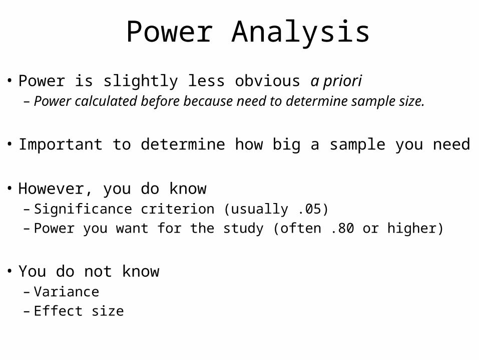
Power Analysis• Power is slightly less obvious a priori
– Power calculated before because need to determine sample size.
• Important to determine how big a sample you need
• However, you do know – Significance criterion (usually .05)– Power you want for the study (often .80 or higher)
• You do not know– Variance– Effect size

Power Analysis
• You do not know– Variance– Effect size
• Step 1 Determine an effect size index
• Step 2 Enter a power table and find n

Power Analysis
• Perhaps the simplest example • An unpaired t-Test with equal variances
Effect size index is:– Difference between the means divided by common standard
deviation
Example• From a previous study (similar to one we are proposing),• Group 1 mean ( 75± 10)awesome• Group 2 mean ( 85± 10)incredible• Difference between means is 10, common SD is 10

Power Analysis
• Difference between means is 10, common SD is 10
• Effect size index is 1.0• Table C.1.2 (P & W) is for a two tailed t-Test
• Enter at the top at effect size 1.0• Go down the column until you get to power you set• Read the n you need in your group

n is the number in each group

What happens if you have a bigger effect size?

What happens if you want better power?

What if…….
• You have unequal variance?• You are doing an ANOVA?• What if it is a correlation study?• Want power for regression analysis?• Power for goodness of fit analysis?• Etc See Appendix C
• What if there are no previous similar studies?
• Guess but with a purpose

Guessing with a purpose (Estimating)
• For a t-test, the effect size index (d) is– .20 for small– .50 for a medium– .80 for a large
• For an ANOVA, the effect size index (f) is– .10 for small– .25 for a medium– .40 for a large
• r for correlation, w for Chi-squared, λ for regression

Power for ANOVA

Power for ANOVA
What if you have only 4 groups?


Regression
• As X changes, does Y?
• X is the independent variable
• Y is the dependent variable
• Regression linea + bX =Ŷ “Y hat”

P & W page 546


SBP (Y) = 64.30 + 1.39 * Age (X)
Y=a+bx64.3 is suppose to be baseline (like at birth)
1.39 is b or rate

Regression Line• Line of best fit• Method of least squares of residuals
• Approximates true regression line of population– Because this done off a sample, not the entire population.
• Assumptions– Normality– Equal variance
• Significance addresses chance, not importance

Outliers in regression
• A convention is ± 3 standard deviations, then it is an outlier.
• What do they represent?– True extremes– Measurement error– Recording errors– Miscalculation– Others?

Accuracy of Prediction• Coefficient of determination– r2 – The amount of variance in Y that can be explained by X– Not the correlation
• Standard Error of the Estimate (SEE)– Standard deviation of the distribution of errors– Variance in the residuals around the regression line• Good example from regression equation for blood pressure
Table 24.3

Linear or Non-Linear?
• Which is the better predictor?– What ever line best fits the data, so depends.
• For a data set– Both have the same total Sum of Squares– One will have higher explained variance– One will have lower explained variance– What is the effect on the ratio?– What is the effect on prediction?

ANCOVA(Briefly)
• Explaining effect of IV on DV• While controlling for confounding variable
– Also can use exclusion criteria.• When there is a covariate (confounding variable) do a ANCOVA
• Assumptions– Linearity of covariate– Homogeneity of slopes– Independence of covariate– Reliability of covariate
• Limitations– Not designed to control for study design weakness– Generalization of data compromised

Χ2
• Non-parametric statistic• Used for frequencies or proportions
– Independent counts– Mutually exclusive and exhaustive categories
• Is there a difference between– Observed frequencies– Expected frequencies
• X2 = ∑ (O – E)2 / E
• Compare to critical values for X2

Χ2 Goodness of fit• Null is that O will not differ from E
• Sample big enough that no expected frequency < 1
• Uniform distributions
• Known distributions
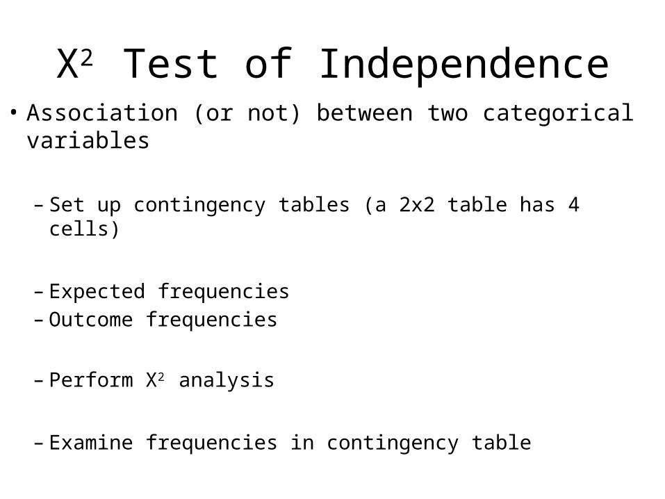
Χ2 Test of Independence• Association (or not) between two categorical variables
– Set up contingency tables (a 2x2 table has 4 cells)
– Expected frequencies– Outcome frequencies
– Perform X2 analysis
– Examine frequencies in contingency table

Χ2 Considerations• Sample size– Each cell has count of at least 1
– No more than 20% of cells have count less than 5
– There are statistical corrections if these aren’t met
• Correlated samples– Violates an assumption that they are independent (because??
Because they are correlated) – McNemar test adjusts for matched or correlated subjects
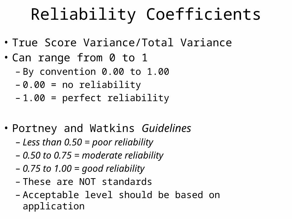
Reliability Coefficients• True Score Variance/Total Variance• Can range from 0 to 1– By convention 0.00 to 1.00– 0.00 = no reliability– 1.00 = perfect reliability
• Portney and Watkins Guidelines– Less than 0.50 = poor reliability– 0.50 to 0.75 = moderate reliability– 0.75 to 1.00 = good reliability– These are NOT standards– Acceptable level should be based on application
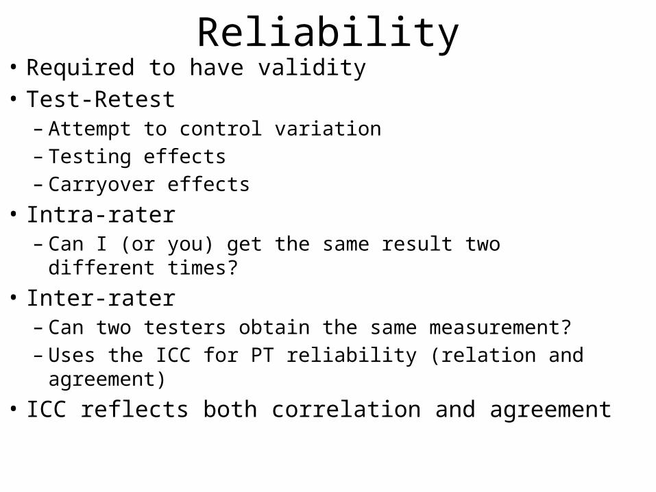
Reliability• Required to have validity• Test-Retest– Attempt to control variation– Testing effects– Carryover effects
• Intra-rater– Can I (or you) get the same result two different times?
• Inter-rater– Can two testers obtain the same measurement? – Uses the ICC for PT reliability (relation and agreement)
• ICC reflects both correlation and agreement
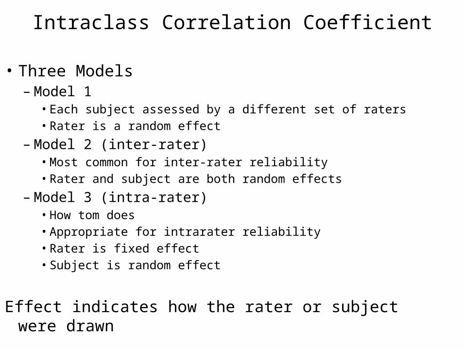
Intraclass Correlation Coefficient
• Three Models– Model 1
• Each subject assessed by a different set of raters• Rater is a random effect
– Model 2 (inter-rater)• Most common for inter-rater reliability• Rater and subject are both random effects
– Model 3 (intra-rater)• How tom does• Appropriate for intrarater reliability• Rater is fixed effect• Subject is random effect
Effect indicates how the rater or subject were drawn

Intraclass Correlation Coefficient
• Two Forms– Form 1• Single ratings
– Form 2• Mean of several (k) measurements
• Nomenclature for Model and Form is– ICC (Model, Form)– i.e. ICC (3,1)

Other reliability indices
• Percent agreement
• Categorical– Percent agreement– Kappa (chance corrected)– Weighted kappa
• Cronbach’s Alpha– Internal consistency
• Correlation of each item to overall correlation• How will each item fits the overall scale

Reliability
• Generalizing– Reliability is not “owned “ by the instrument– May not apply to:• Another population• Another rater (or group of raters)• Different time interval
• Minimum Detectable Difference– Or minimum detectable change– How much change is needed to say it’s not chance– Not the same as MCID

Standard error of the measurement (SEM)?
• An indication of the precision of the score • Product of the standard deviation of the data
set and the square root of 1-ICC• Used to construct a CI around a single
measurement within which the true score is estimated to lie
• 95% CI around the observed score would be: Observed score ± 1.96*SEM
Weir JP. Quantifying test-retest reliability using the intraclass correlation coefficient and the SEM. J Strength Cond Res. Feb 2005;19(1):231-240.

Validity Truth
Test+
+
-
Sp
Sn
a b
c d
1-Sn = - LR
+ LR = 1-Sp
Sp = d/b+d
Sn = a/a+c

Phrases to Know• Power is the ability of a statistical test to find a significant difference that really
does exist. – probability that test will lead to a rejection of the null.
• P-value shows the probability that the difference you found was not by chance. • Null hypothesis is that there is no difference or change• Type I error is an incorrect decision to reject the null, concluding that a
relationship exist when in fact it does NOT.• Type II error is an incorrect decision to accept the null, concluding that no
relationship exists when in fact one does. • Sn is a measure of validity of a screening procedure, based on the probability
that someone WITH the disease will test positive• Sp is a measure of validity of a screening procedure, based on the probability
that some that does NOT have the disease will test negative. • Etc (sample questions sent from your classmates posted today)


