
Party Bias in Union Representation Elections:Testing for Manipulation in the RegressionDiscontinuity Design When the Running
Variable is Discrete
Brigham R. FrandsenBrigham Young UniversityDepartment of Economics
September 16, 2016
Abstract
Conventional tests of the regression discontinuity design’s identifyingrestrictions can perform poorly when the running variable is discrete.This paper proposes a test for manipulation of the running variable thatis consistent when the running variable is discrete. The test exploitsthe fact that if the discrete running variable’s probability mass functionsatisfies a certain smoothness condition, then the observed frequency atthe threshold has a known conditional distribution. The proposed testis applied to vote tally distributions in union representation electionsand reveals evidence of manipulation in close elections that is in favor ofemployers when Republicans control the NLRB and in favor of unionsotherwise.
1 Introduction
The regression discontinuity (RD) design, a research strategy that exploits
plausibly exogenous variation in a treatment assigned via a threshold or cut-
off rule, has become one of the most frequently used tools in the empirical
economist’s kit. Originally developed for, and still commonly applied to eval-
uation of education interventions, where threshold-based rules are the norm,
1

RD designs have found wide application in labor economics, public finance,
environmental economics, political economy, and other diverse settings (see
van der Klaauw, 2008 for a survey).
There is good reason for the RD design’s popularity. First, in settings
where it can be verified, the RD design appears to make good on its promise
of delivering unbiased estimates of causal effects. Estimates from RD designs
agree with their close cousins, randomized experiments, in numerous within-
study comparisons where both methods are available (Buddelmeyer and Sk-
oufias, 2003; Black et al., 2007; Cook and Wong, 2008). Another attraction
of the RD design lies in the ability to transparently test the plausibility of
its identifying assumptions. The RD design relies on the assumption that in-
dividuals immediately on either side of a threshold—for example, with test
scores just above and below a cutoff—are comparable. This is plausible if in-
dividuals cannot precisely manipulate their score. One test of the identifying
assumption looks for red flags that individuals are, in fact, manipulating their
score by examining the distribution near the RD threshold for discontinuities
in the density that would point to manipulation or confounding selection. Mc-
Crary’s (2008) test exploits this idea using local linear regression of histogram
frequencies at the threshold. This test has become part of the recommended
battery of analyses for RD practitioners (Imbens and Lemieux, 2008; Lee and
Lemieux, 2010). Cattaneo et al. (2016) propose a similar test based on local
linear regression estimates of the density, but avoiding the initial histogram
step.
Like the standard RD identifying assumptions in Hahn et al. (2001), this
widely used test assumes the running variable is continuously distributed. In
practice, however, many regression discontinuity designs employ a discrete
running variable.1 When the running variable has a finite number of fixed
1Some examples of regression discontinuity designs based on discrete running variablesin the recent literature include the effects of class size based on primary school enrollment(Angrist and Lavy, 1999), the effects of unionization using representation election voteshare bins (DiNardo and Lee, 2004; Lee and Mas, 2012; Frandsen, 2015), the effects ofMedicaid eligibility based on age in months (Card and Shore-Sheppard, 2004), the effect ofPre-K programs using age (Gormley et al., 2005), the effects of summer school on studentachievement using discrete test scores (Matsudaira, 2008), the effects of Medicare usingage in quarters or years (Card et al., 2009; Chay et al., 2010) , and the effects of collegescholarships on student outcomes using categorical test scores (DesJardins et al., 2010).
2
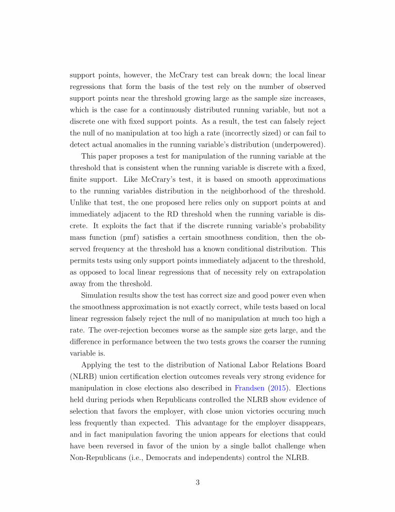
support points, however, the McCrary test can break down; the local linear
regressions that form the basis of the test rely on the number of observed
support points near the threshold growing large as the sample size increases,
which is the case for a continuously distributed running variable, but not a
discrete one with fixed support points. As a result, the test can falsely reject
the null of no manipulation at too high a rate (incorrectly sized) or can fail to
detect actual anomalies in the running variable’s distribution (underpowered).
This paper proposes a test for manipulation of the running variable at the
threshold that is consistent when the running variable is discrete with a fixed,
finite support. Like McCrary’s test, it is based on smooth approximations
to the running variables distribution in the neighborhood of the threshold.
Unlike that test, the one proposed here relies only on support points at and
immediately adjacent to the RD threshold when the running variable is dis-
crete. It exploits the fact that if the discrete running variable’s probability
mass function (pmf) satisfies a certain smoothness condition, then the ob-
served frequency at the threshold has a known conditional distribution. This
permits tests using only support points immediately adjacent to the threshold,
as opposed to local linear regressions that of necessity rely on extrapolation
away from the threshold.
Simulation results show the test has correct size and good power even when
the smoothness approximation is not exactly correct, while tests based on local
linear regression falsely reject the null of no manipulation at much too high a
rate. The over-rejection becomes worse as the sample size gets large, and the
difference in performance between the two tests grows the coarser the running
variable is.
Applying the test to the distribution of National Labor Relations Board
(NLRB) union certification election outcomes reveals very strong evidence for
manipulation in close elections also described in Frandsen (2015). Elections
held during periods when Republicans controlled the NLRB show evidence of
selection that favors the employer, with close union victories occuring much
less frequently than expected. This advantage for the employer disappears,
and in fact manipulation favoring the union appears for elections that could
have been reversed in favor of the union by a single ballot challenge when
Non-Republicans (i.e., Democrats and independents) control the NLRB.
3

Methodologically, this paper is related to previous work on the problems
posed by RD designs when the running variable is discrete. Lee and Card
(2008) show that discrete running variables induce specification errors that
can be accounted for in the inference procedure they propose. Kolesar and
Rothe (2016) develop an alternative inference procedure for discrete running
variables with superior theoretical properties. Dong (2012) develops a bias-
corrected estimation procedure to account for rounding error when the discrete
running variable is a rounded version of an underlying continuous variable.
The current paper complements this previous work on RD estimation and
inference in the case of discrete running variables by developing a test of the
identifying conditions that can then justify using those tools. This paper also
complements work by Gerard et al. (2015), who consider partial identification
in RD designs when manipulation is present.
The testing approach is also related to the finite-sample nonparametric
literature on inference for approximately linear functions. The test in this
paper is based on a smoothness condition that puts a bound on the finite
analog to the second derivative of the running variable’s pmf, and derives sharp
bounds on the distribution of the test statistic. This approach of performing
inference within a functional class defined by bounds on derivatives is also
followed by Armstrong and Kolesar (2015) but dates back at least to Sacks
and Ylvisaker (1978).
The test proposed in this paper may also be of interest outside of a re-
gression discontinuity setting. It can be applied to settings where detecting
sorting or heaping along a discretely-measured dimension is important. For
example, the methodology could be used to test behavioral theories that im-
ply bunching or sorting relative to pre-determined benchmarks or norms, such
as round numbers in SAT scores or batting averages (Pope and Simonsohn,
2011). The test could also be used to quantify distortions in firm behavior
in response to policies based on firm-size thresholds, such as the Family and
Medical Leave Act and the Affordable Care Act in the United States or em-
ployment protection laws in Europe (Waldfogel, 1999; Garibaldi et al., 2004;
Schivardi and Torrini, 2008). In applications such as these, the results of the
test are of interest in their own right, and not just as specification checks.
4

2 Econometric framework
Consider a standard regression discontinuity design in which an individual’s
treatment assignment, D, depends on whether a scalar-valued continuously
distributed variable R∗, referred to as the running variable or forcing variable,
exceeds some known threshold normalized to zero. Treatment assignment can
therefore be written as
D = 1 (R∗ ≥ 0) .
For example, R∗ might be the difference between an individual’s age and the
Medicare eligibility threshold, 65. Let the potential outcome if the individual
were not to receive the treatment be Y (0) and if he or she were to receive the
treatment, Y (1). The observed outcome is therefore
Y = Y (0) (1−D) + Y (1)D.
The estimands of interest in the regression discontinuity design are typi-
cally the distributions of Y (0) and Y (1) conditional on R∗ = 0 or function-
als of those distributions such as the conditional average treatment effect at
the threshold, E [Y (1)− Y (0) |R∗ = 0]. The following standard continuity
assumption is sufficient to identify the conditional average treatment effect
(Hahn et al., 2001; Frandsen et al., 2012):
Assumption 1 Regarded as functions of r, E [Y (0) |R∗ = r] and E [Y (1) |R∗ = r]
are continuous at zero.
This assumption rules out discrete jumps in unobservables at the thresh-
old, so that any observed jump in outcomes there can be attributed to the
effects of treatment. It implies that individuals immediately on either side
of the threshold are comparable. It is analogous to the conditional indepen-
dence assumptions underpinning standard regression analysis or the exclusion
restriction invoked in instrumental variables analysis. The assumption is more
plausible when the running variable cannot be chosen or manipulated precisely
by the individual. For example, the assumption would be satisfied if R∗ were
randomly assigned and it had no effect on outcomes other than through its
determination of treatment status.
5

2.1 Standard Tests for Running Variable Manipulation
The RD identifying assumption cannot be tested directly since Y (0) and Y (1)
are observable on only one side of the threshold or the other. However, plau-
sible rationales for this assumption imply that the density of R∗ should be
continuous at zero. For example, suppose R∗ can be partially influenced by
the individual; one would then expect selection differences to arise on average
between treated and untreated individuals. But if R∗ has a random component
that cannot be precisely manipulated, one would expect individuals immedi-
ately on either side of the threshold to be comparable—that is, Assumption 1
should be satisfied (Lee, 2008). A discontinuity in the density of the running
variable at the threshold raises a red flag that perhaps individuals can pre-
cisely manipulate the running variable after all, and therefore individuals on
either side of the threshold may not be comparable.
The idea that anomalies in the running variable at the threshold signal
violations of Assumption 1 forms the basis of McCrary’s (2008) test, which
examines the estimated density of the running variable on either side of the
threshold, and has become part of the standard battery for RD practitioners
(Imbens and Lemieux, 2008; Lee and Lemieux, 2010). The McCrary test con-
sists of two steps. The first step constructs the running variable’s histogram
using bins of width bn, which become narrower as the sample size increases.
The second step performs kernel-weighted linear regressions of the log of the
histogram frequencies on either side of the threshold using a bandwidth hn—
which also shrinks with the sample size—and tests for a difference in inter-
cepts. A significant difference points to a discontinuity in the running variable
density at the threshold, suggesting possible manipulation and violations of
Assumption 1.
Cattaneo et al. (2016) propose a test similar in spirit that also tests for
differences in local polynomial regression estimates of the density on either
side of boundary. This test avoids the initial binning step and instead per-
forms kernel-weighted polynomial regressions of jack-knifed estimates of the
empirical cdf.
Both of these tests perform well in terms of size and power in standard RD
settings where the running variable’s distribution is well approximated by a
continuous distribution.
6

2.2 Discrete Test for Running Variable Manipulation
Suppose now that instead of R∗, we observe a discrete running variable, R
satisfying the following property:
Assumption 2 R has finite support on points at equally spaced intervals of
length ∆ > 0.
The discrete running variable R may be taken to be a rounded version
of an underlying continuous variable—for example, R = bR∗/∆rc∆r, as in
age measured in years (Card et al., 2009)—or a naturally discrete variable
such as primary school enrollment (Angrist and Lavy, 1999). As above, the
treatment threshold’s location is normalized so the smallest treated support
point is defined to be zero. The intuitive implication of standard RD sufficient
identifying conditions that the pmf should be smooth at the threshold still
provides the basis for the proposed manipulation test when the observed run-
ning variable is discrete. In our smoothness notion, however, finite differences
replace derivatives , since our random variable has finite support. Define the
second-order finite difference of a function f at a point r as
∆(2)f (r) :=f (r + ∆)− 2f (r) + f (r −∆)
∆2,
which corresponds to the finite analog of a second derivative. The smoothness
condition corresponding to the hypothesis of no manipulation in the discrete
case is the following:
Assumption 3 R has a probability mass function f (r) with a bounded second-
order finite difference at zero that satisfies
∣∣∆(2)f (0)∣∣ ≤ k
f (−∆) + f (∆)
∆2,
for known k ≥ 0.
Assumption 3 is a finite analog to the standard smoothness condition in-
voked in, for example, Armstrong and Kolesar (2015), but with the smooth-
ness constant on the right-hand side scaled by (f (−∆) + f (∆)) /∆2 to ensure
the test statistic defined below is pivotal. The scaling makes no restriction
7

on the class of admissible functions for f beyond a bounded second-order
finite difference; for example, suppose the absolute value of the second fi-
nite difference were bounded by C. Then define k in Assumption 3 to be
C∆2/ (f (−∆) + f (∆)). Since f is by definition positive at −∆ and ∆, this
makes no further restriction. Like the inference method proposed in Armstrong
and Kolesar (2015), the test proposed here requires the researcher to choose
a value for k. One possible difference is in Armstrong and Kolesar’s (2015)
setting, a conservative choice for the bounding constant does not substantially
harm efficiency, which may not be the case here.
Assumption 3 is akin to the local linear approximation in traditional RD
settings with a continuously distributed running variable. The smoothness re-
quirement captures the notion of no manipulation as in McCrary (2008). The
requirement that it have bounded finite difference is analogous to the differ-
entiability required for RD estimation and inference (Hahn et al., 1999). As-
sumption 3 differs from the conventional assumptions in two important ways,
however. First, the condition makes restrictions not only at the threshold, but
over a fixed neighborhood. This is a fact of life for discrete running variables;
the fixed support points preclude the nonparametric approach of a vanish-
ing bandwidth around the threshold. Second, the condition requires that the
bound coefficent, k, be specified. The choice of k determines the degree of
departure from linearity around the threshold beyond which manipulation is
implied. For example, choosing k = 0 specifies that a distribution compatible
with no manipulation must be precisely linear around the threshold. Choosing
a larger k allows a degree of nonlinearity at the threshold without concluding
manipulation. As discussed below, a smaller k leads to a more powerful test,
but may also detect manipulation when none is present.
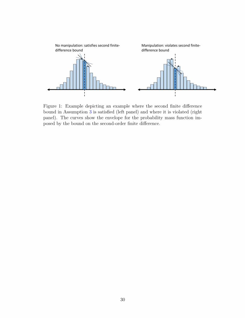
Figure 1 illustrates the role of Assumption 3. The left-hand panel, meant
to depict a case with no manipulation, shows that f (r) satisfies the bound on
the second-order finite difference whose envelope is indicated by the curves.
The right-hand panel shows an example with manipulation, in which the pmf’s
nonlinearity exceeds the bounds on the second-order finite difference.
The basis of the test is the observation that when Assumption 3 is satisfied
the observed sample frequency at R = 0 has a known distribution conditional
on R ∈ {−∆, 0,∆}, as the following theorem shows.
8

Theorem 1 Suppose Assumption 3 is satisfied. Then
Pr (R = 0|R ∈ {−∆, 0,∆}) ∈[
1− k3− k
,1 + k
3 + k
].
Proof. All proofs are in the Appendix.
The result says that if f (r) is sufficiently smooth at the threshold, then
conditional on R taking on a value at the threshold or an immediately adjacent
support point, the probability of being exactly at the threshold is between
(1− k) / (3− k) and (1 + k) / (3 + k). For k = 0 this implies the probability
is exactly 1/3. The theorem is exact; the result holds no matter how small the
sample.
The intuition for the result is the same as for the McCrary test. If the
distribution is smooth then it admits a linear approximation in the neighbor-
hood of the threshold. It turns out that in the linear case with k = 0, then
Pr (R = 0|R ∈ {−∆, 0,∆}) = 1/3 is not only necessary but also sufficient for
the “no-manipulation” Assumption 3 to hold. The appendix shows this intu-
ition formally.
The theorem’s result and its antithesis constitute the null and alternative
hypotheses for the proposed test:
H0 : Pr (R = 0|R ∈ {−∆, 0,∆}) ∈ P (k) :=
[1− k3− k
,1 + k
3 + k
];
H1 : Pr (R = 0|R ∈ {−∆, 0,∆}) ∈ (0, 1) \ P (k) ,
for known k.
2.2.1 Test Statistic, Null Distribution, Critical Values, and Power
Given an iid sample of size n from the distribution ofR, letNr :=∑n
i=1 1 (Ri = r)
be the sample frequency at R = r, where r ∈ {. . . ,−∆, 0,∆, . . .}. The test
statistic is N0, the observed sample frequency at Ri = 0. The following corol-
lary to Theorem 1 gives the test statistic’s distribution under the null hypoth-
esis:
Theorem 2 Suppose {Ri}ni=1 are independent and identically distributed sam-
ples of R satisfying Assumption 2. Then under H0 and conditional on m =
9

N−∆ +N0 +N∆,
N0 :=n∑i=1
1 (Ri = 0) ∼ B (m, p) ,
where B (m, p) denotes a Binomial random variable with number of trials m
and probability of success p ∈ P (k).
Since the null hypothesis specifies a set for the parameter p, simply in-
verting the Binomial cdf at a given p does not produce uniformly valid critical
values. Instead, the following theorem constructs critical values that uniformly
control size over P (k):
Theorem 3 Suppose {Ri}ni=1 are independent and identically distributed sam-
ples of R satisfying Assumption 2. Then under H0,
Pr(CLα (k) < N0 < CU
a (k) |N−∆ +N0 +N∆ = m)≥ 1− α,
where CLα (k) and CU
α (k) are values in {0, . . . ,m} that solve the following dis-
crete minimization problem:
minCL,CU
∣∣CU − CL∣∣
s.t. infp∈P(k)
FB(CU − 1;m, p
)− FB
(CL;m, p
)≥ 1− α,
and FB is the Binomial cdf:
FB (x;m, p) :=
bxc∑j=1
(m
j
)pj (1− p)m−j .
The theorem establishes that under H0 a test that fails to reject when N0
is strictly between the upper and lower critical values, and rejects otherwise
will have size uniformly controlled by α. By minimizing the length of the
non-rejection region the test maintains good power against alternatives that
deviate from H0 in either direction. The following result establishes that the
test is consistent against any fixed alternative H1.
Theorem 4 Suppose {Ri}ni=1 are independent and identically distributed sam-
ples of R satisfying Assumption 2. Suppose H1 holds with either Pr (R = 0|R ∈ {−∆, 0,∆}) =
10

1−k3−k − δ or Pr (R = 0|R ∈ {−∆, 0,∆}) = 1+k
3+k+ δ for some δ > 0. Then the
probability of rejection approaches unity as the sample size increases.
2.2.2 Including additional support points
The proposed test relies on three support points of the discrete running vari-
able. The choice of three is not arbitrary. In principle, a similar test could be
constructed using observed frequencies from any odd-numbered (but greater
than one) set of support points arranged symmetrically about the threshold.
Specifically, consider a test based on an odd number 2d + 1 support points
(d = 1, 2, 3, . . .), the middle one of which is located at the threshold. Assump-
tion 3 implies that the conditional probability of R = 0, conditional on R
taking on one of the 2d+ 1 values is
Pr (R = 0|R ∈ {−d∆, . . . , d∆}) ∈
[1− k
∑ds=1 s
2
2d+ 1− k∑d
s=1 s2,
1 + k∑d
s=1 s2
2d+ 1 + k∑d
s=1 s2
].
The choice of d = 1 (three support points) is preferred for two reasons. First, it
requires invoking the smoothness condition over the smallest possible interval,
where it is most likely to be reasonable. Second, for a given choice of k,
increasing the number of points quickly leads to a test with no power: the
lower bound of the null set approaches zero, and the upper bound approaches
one.
2.2.3 Choosing k
Researchers must choose the parameter k ≥ 0 in order to implement the test.
The choice of k determines the maximal degree of nonlinearity in the pmf that
is still considered to be compatible with no manipulation. A large k means the
mass at the threshold can deviate substantially from linearity before the test
will reject with high probability, while a small k means even small deviations
from linearity will lead the test to reject with high probability. Choosing
k to be conservatively high will therefore reduce the test’s power to detect
manipulation. How should researchers choose k? The choice clearly cannot
be driven by the data used in the test—that is, observations adjacent to the
threshold. The degree of curvature in benchmark distributions may be used to
11

generate rules of thumb. For example, if the running variable were a discretized
version of a normally distributed random variable, discretized to coarseness ∆
in units of the standard deviation, then the maximal degree of curvature, as a
function of ∆, corresponds to a k given by the following expression:
kmaxN (∆) =
∆3φ (∆/2)
2 (Φ (3∆/2)− Φ (∆/2)),
where φ and Φ are the standard normal density and cdf. The maximal k
is increasing in the coarseness. For ∆ = .1, which corresponds to about 20
support points within one standard deviation of the threshold, the maximal k
is 0.005. For ∆ = .3, a very coarse discretization with only about six support
points within one standard deviation, the maximal k is 0.047. A researcher
could alternatively take a rule of thumb from the observed distribution of
the running variable away from the threshold, but keeping the following in
mind: (1) no manipulation can be present elsewhere in the distribution; (2) the
degree of curvature elsewhere in the distribution must be informative about the
curvature at the threshold; (3) the test then must be taken to be conditional
on the observed running variable distribution away from the threshold.
2.3 The McCrary test with discrete data
The McCrary (2008) test, outlined in Section 2.1, generally performs well—
that is, it has approximately correct size and good power—when the running
variable is continuous, but it can deteriorate when the running variable is
discrete.
Nevertheless, the test can be applied to discrete data by taking the support
points of the running variable to be the histogram bins, and running a kernel-
weighted local linear regression of the log of the observed frequencies on either
side of the threshold.
Why might the McCrary test perform poorly with discrete data, when
its first step is, in fact, to discretize the running variable? The answer is
that the McCrary procedure consistently tests whether two estimands—linear
extrapolations of the (log) pmf to the threshold from the left and right—are
equal, but equality of those estimands is neither necessary nor sufficient for the
12

no-manipulation smoothness condition in a setting with fixed support points.
When the running variable is continuously distributed and the discretization
can home in on the threshold as the sample size increases, then equality of
the two estimands implies the density is continuous, and the test is consistent,
but with a discretely distributed running variable the McCrary procedure can
lead to over- or under-rejection of the smoothness condition.
There is an exception, however: if the underlying pmf truly is exactly linear
away from the threshold, the McCrary test will be consistent even in a discrete
setting, and may have more power, but exact linearity is a strong assumption
not commonly made in RD settings, and embodies more than the hypothesis
of no manipulation would seem to imply.
3 Simulations
This section numerically illustrates the theoretical results above concerning
the test’s size and power.
The first set of simulations illustrates the performance of the test over
a range of sample sizes when k is chosen correctly. The running variable
is a binned version of an underlying continuous random variable. Let the
underlying random variable be R∗ ∼Log-N (µ, σ2), and let the discrete running
variable based on this be R = b(R∗ − rc) /∆c×∆+rc, where rc is the threshold,
and ∆ is the support point spacing. The threshold will be placed so that the
mode of the distribution, m = exp (µ− σ2) is exactly between the treated and
untreated support points, that is, rc = m+∆/2. For the baseline specification
of µ = 0, σ2 = 1, and ∆ = .1, the value of k is .02. All simulations are based on
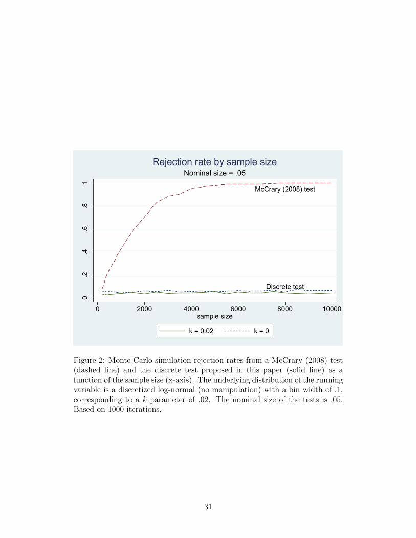
1,000 iterations. Figure 2 plots simulated rejection rates for sample sizes from
n = 200 to n = 10, 000, with running variable distribution parameters µ = 0,
σ2 = 1, and ∆ = .1. In this scenario there is no manipulation, so a correctly
sized test should reject at a rate equal to the nominal size, α = .05. The solid
line corresponds to the discrete test with a correctly specified k, and shows that
the rejection rate hovers right around the nominal 5 percent. The figure also
shows that the McCrary test rejects at only slightly more than the nominal
rate at the lowest sample size, but the rejection rate quickly approaches 100
percent for sample sizes above 5,000.
13
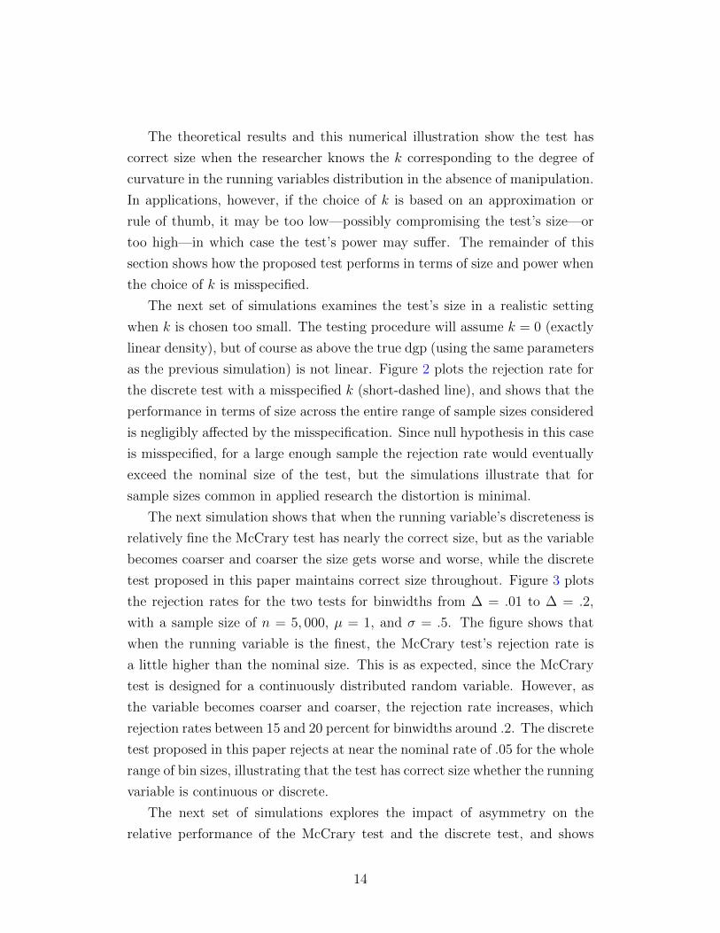
The theoretical results and this numerical illustration show the test has
correct size when the researcher knows the k corresponding to the degree of
curvature in the running variables distribution in the absence of manipulation.
In applications, however, if the choice of k is based on an approximation or
rule of thumb, it may be too low—possibly compromising the test’s size—or
too high—in which case the test’s power may suffer. The remainder of this
section shows how the proposed test performs in terms of size and power when
the choice of k is misspecified.
The next set of simulations examines the test’s size in a realistic setting
when k is chosen too small. The testing procedure will assume k = 0 (exactly
linear density), but of course as above the true dgp (using the same parameters
as the previous simulation) is not linear. Figure 2 plots the rejection rate for
the discrete test with a misspecified k (short-dashed line), and shows that the
performance in terms of size across the entire range of sample sizes considered
is negligibly affected by the misspecification. Since null hypothesis in this case
is misspecified, for a large enough sample the rejection rate would eventually
exceed the nominal size of the test, but the simulations illustrate that for
sample sizes common in applied research the distortion is minimal.
The next simulation shows that when the running variable’s discreteness is
relatively fine the McCrary test has nearly the correct size, but as the variable
becomes coarser and coarser the size gets worse and worse, while the discrete
test proposed in this paper maintains correct size throughout. Figure 3 plots
the rejection rates for the two tests for binwidths from ∆ = .01 to ∆ = .2,
with a sample size of n = 5, 000, µ = 1, and σ = .5. The figure shows that
when the running variable is the finest, the McCrary test’s rejection rate is
a little higher than the nominal size. This is as expected, since the McCrary
test is designed for a continuously distributed random variable. However, as
the variable becomes coarser and coarser, the rejection rate increases, which
rejection rates between 15 and 20 percent for binwidths around .2. The discrete
test proposed in this paper rejects at near the nominal rate of .05 for the whole
range of bin sizes, illustrating that the test has correct size whether the running
variable is continuous or discrete.
The next set of simulations explores the impact of asymmetry on the
relative performance of the McCrary test and the discrete test, and shows
14

that as the distribution of the running variable becomes more skewed, the
McCrary test performs more poorly, while the discrete test maintains good
properties. The simulation varies skewness, but holding the variance V =
(expσ2 − 1) exp (2µ+ σ2) constant at the level in the first set of simulations,
with µ = 0 and σ = 1 in order to isolate the impact of skewness. This was
achieved by varying σ from .05 to 1 (corresponding to skewness from about
.15 to over 6), and setting µ = −12
(ln(
1V
(expσ2 − 1))
+ σ2)
to hold the vari-
ance constant. Skewness depends on the value of σ2 via the following formula:
γ1 = (expσ2 + 2)√
expσ2 − 1. The support point spacing is set at ∆ = .1
as in the first set of simulations. Figure 4 plots the rejection rates for the
two tests for skewness parameters from .15 to over 6, with a sample size of
n = 3, 000. The figure shows that for skewness values below one, both tests
perform similarly with rejection rates very close to the nominal .05. As skew-
ness increases, however, the McCrary test rejects more and more frequently,
exceeding 80 percent when skewness reaches six.
The previous sets of simulations showed that when the running variable is
discrete the McCrary test can falsely reject the null hypothesis at much too
high a rate, while the discrete test has approximately correct size even when
k is chosen too small. As noted above, the test’s good size under misspecifi-
cation is a finite-sample phenomenon: for a large enough sample even small
misspecifications will lead to size distortions. A relevant question, then, is
whether for the range of sample sizes in which the misspecified test maintains
correct size it still has power to detect manipulation. The next set of simula-
tions answers this question. The underlying continuous variable will be altered
by introducing a probability of switching from below the threshold to above,
where the probability of switching increases near the threshold. To be precise,
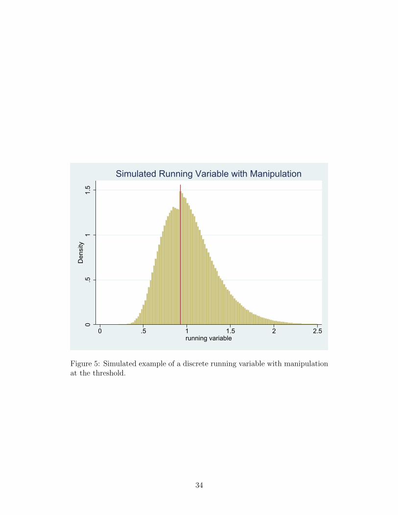
the altered underlying continuous variable will be R defined as follows:
R = R∗ + 2 (rc −R∗)S,
S ∼ Bernoulli (p (r)) |R∗ = r,
p (r) = β exp (−γ |r − rc|)× 1 (R∗ < rc) ,
R∗ ∼ log-N(µ, σ2
).
The discretized running variable will then simply be R =⌊(R− rc
)/∆⌋×
15

∆ + rc. Figure 5 shows an example of what the resulting distribution looks
like.
The first power simulation shows the test’s rejection rate is minimized
where the probability of manipulation is zero (so the test is unbiased) and
the power is greater when the probability of manipulation is higher. Figure
6 plots the rejection rate of the test as a function of β, the maximum proba-
bility of manipulation (or switching) at the threshold, and, for reference, the
rejection rate of the McCrary test. The running variable’s true distribution
has parameters µ = 0, σ = 1, ∆ = .1, γ = 1, and n = 1000. The discrete
test’s rejection rate is at the nominal size of .05 when β = 0, as it should
be since there the null hypothesis of no manipulation is true. The rejection
rate monotonically increases as the probability of manipulation gets higher,
reaching 80 percent when β ≈ .4 and 90-100 percent when β = .6 and higher.
The figure also shows for reference that the unadjusted McCrary test rejects
at a higher-than-nominal rate even when there is no manipulation, as previous
simulations showed. Adjusting the McCrary test by calculating critical values
that give correct rejection rates when β = 0 (see Lloyd, 2005) makes the power
remarkably close to the discrete test’s.
The next simulation shows the discrete test is more powerful when the
running variable is “more discrete,” that is, when the running variable’s dis-
tribution is coarser. Figure 7 plots the test’s rejection rate as a function of
the bin width, ∆, fixing the maximum probability of manipulation at β = .5,
with the other simulation parameters as in the simulation exploring the test’s
size as a function of ∆: n = 5, 000, µ = 1, and σ = .5. The figure shows that
for the narrowest bins the test has power of about 40 percent, and the power
increases rapidly as the bin width gets larger, reaching 80 percent when the
bin width is about .04 and higher, and about 100 percent when the bin width
is about .1 and higher. This is as expected, since for a fixed sample size, when
the bins are larger there are more observations at the threshold and adjacent
support points. The trade off, of course, is that when the running variable is
very coarse, the smoothness approximation may be less exact, even when there
is no manipulation, leading to incorrect size. The earlier simulations (Figure
3) showed that over this range, however, the test maintains correct size.
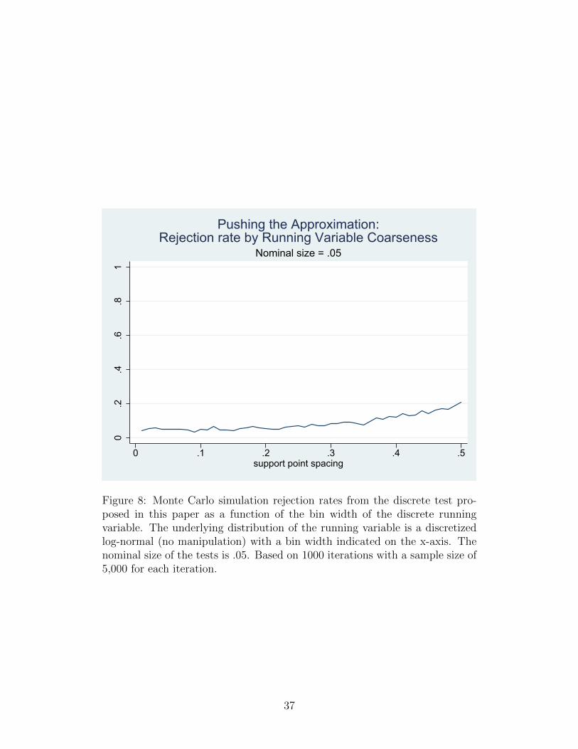
The next simulation pushes the limits of the approximation (k = 0) to
16

show when the test’s performance breaks down. The simulation computes the
size of the test as a function of the coarseness of the running variable, but
over a wider range than in Figure 3, to show at what point the test begins
to significantly over-reject. Figure 8 plots the rejection rate for binwidths
from ∆ = .01 to ∆ = .5, with the other parameters set as in Figure 3. The
corresponding true values for k range from 4.4 × 10⁻⁵ (for ∆ = .01) to .044
(for ∆ = .5). The upper bound on coarseness of .5 corresponds to a discrete
running variable with only 4-5 support points below the threshold and 20-23
above, much coarser than the discrete running variables used in the studies
cited in the introduction. The plot shows that for running variables with a
support finer than around .25 the test rejects at very near the nominal rate of
5 percent. For coarseness beyond this point, however, the test begins to over-
reject as the approximation becomes less accurate, reaching about 20 percent
for support spacing of .5. Thus, while the test breaks down for extremely coarse
running variables, it performs well even beyond the range of discreteness seen
in practice.
The previous sets of simulations showed that specifying k to be too low—
while theoretically compromising the size of the test for a large enough sample
size—introduces little size distortion for most typical parameter ranges, but
can lead to problems with extremely coarse running variables. What are the
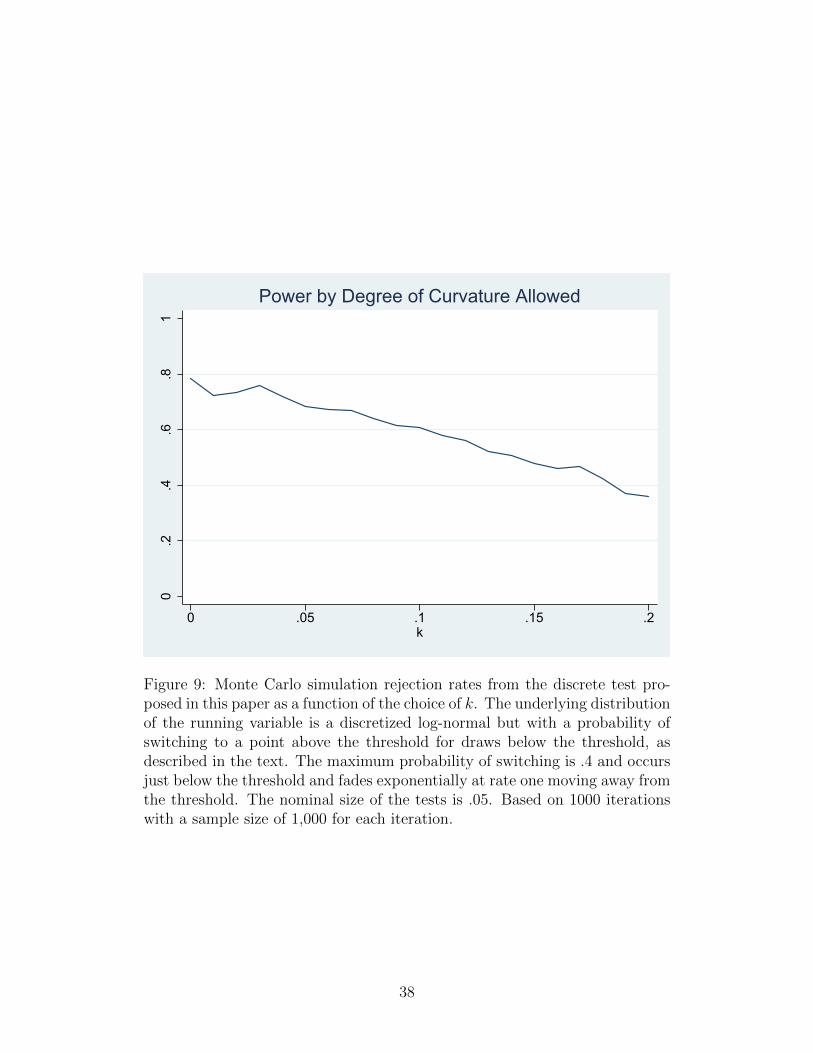
consequences of choosing larger values for k? The next simulation answers this
question. This simulation sets the running variable distribution’s parameters
to µ = 0, σ = 1, ∆ = .1, γ = 1, and n = 1000, and introduces manipulation as
before with β = .4, where the test with k = 0 has power of about 80 percent
in the earlier simulations. This simulation considers a range for k from zero
to .2. Figure 9 plots the test’s power as a function of k. The test’s power
decreases as k increases, since larger and larger departures from linearity are
still considered consistent with no manipulation as k grows. The power at
k = 0 is about 80 percent, but decreases to 36 percent at k = .2.
To summarize, the simulation results showed that in a setting based on the
log-normal distribution the discrete test maintains correct size even when k is
chosen to be too small, and appears to have good power properties. Choosing
larger and larger k decreases the test’s power.
17

4 Empirical Example
The regression discontinuity design has been an important tool for studying
the impacts of unions on business establishments (DiNardo and Lee, 2004;
Lee and Mas, 2012). This strategy exploits the fact that most private sec-
tor unions in the United States form via secret ballot representation elections
among workers at the establishment who will be part of the potential bargain-
ing unit. Since 1935, these elections have been overseen by the National Labor
Relations Board (NLRB), which certifies the union as the sole authorized bar-
gaining representative of the workers in the unit if the union obtains a strict
majority of the votes. Thus, in close elections, very small differences in vote
tallies determine whether an establishment will become unionized or not. If
establishments and workers where the union barely wins and barely loses are
comparable, then comparisons of post-election outcomes will reflect the causal
impact of unionization.
The critical assumption is that the final vote tally in close elections is not
manipulable by the union or the employer. One threat to this condition could
occur in elections involving a small number of voters, when unions or employ-
ers might have more precise knowledge about the likely voting outcomes, and
perhaps more influence over the individual voting decisions. In part to over-
come this threat, it is common practice in this setting to restrict analysis to
elections involving at least 20 voters (DiNardo and Lee, 2004; Frandsen, 2015).
However, even elections involving a large number of voters may be sub-
ject to manipulation. The institutional rules governing union representation
elections allow for ex post challenges to individual ballots. In elections that
come down to a single vote, the losing side would have a great incentive to
challenge an opposing vote and use whatever influence it could to have the
NLRB throw the ballot out. This kind of manipulation could possibly intro-
duce confounding selection even in close elections involving a large number of
voters. Frandsen (2015) shows evidence for just this sort of selection.
This empirical example illustrates the proposed test for manipulation by
examining the possibility that the degree of influence unions and employers
can have on the outcome of close elections could depend in part on which
party controls the NLRB. Evidence for this kind of partisan bias using other
18
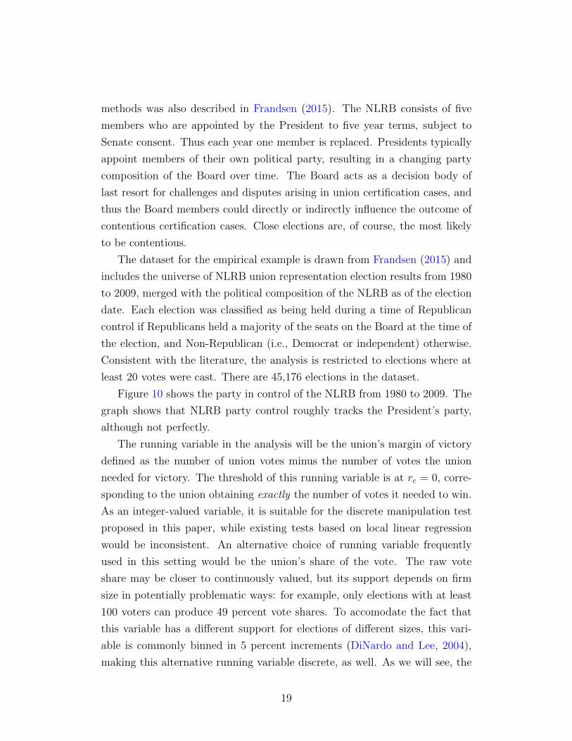
methods was also described in Frandsen (2015). The NLRB consists of five
members who are appointed by the President to five year terms, subject to
Senate consent. Thus each year one member is replaced. Presidents typically
appoint members of their own political party, resulting in a changing party
composition of the Board over time. The Board acts as a decision body of
last resort for challenges and disputes arising in union certification cases, and
thus the Board members could directly or indirectly influence the outcome of
contentious certification cases. Close elections are, of course, the most likely
to be contentious.
The dataset for the empirical example is drawn from Frandsen (2015) and
includes the universe of NLRB union representation election results from 1980
to 2009, merged with the political composition of the NLRB as of the election
date. Each election was classified as being held during a time of Republican
control if Republicans held a majority of the seats on the Board at the time of
the election, and Non-Republican (i.e., Democrat or independent) otherwise.
Consistent with the literature, the analysis is restricted to elections where at
least 20 votes were cast. There are 45,176 elections in the dataset.
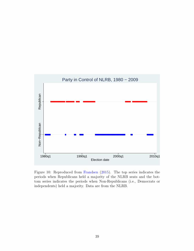
Figure 10 shows the party in control of the NLRB from 1980 to 2009. The
graph shows that NLRB party control roughly tracks the President’s party,
although not perfectly.
The running variable in the analysis will be the union’s margin of victory
defined as the number of union votes minus the number of votes the union
needed for victory. The threshold of this running variable is at rc = 0, corre-
sponding to the union obtaining exactly the number of votes it needed to win.
As an integer-valued variable, it is suitable for the discrete manipulation test
proposed in this paper, while existing tests based on local linear regression
would be inconsistent. An alternative choice of running variable frequently
used in this setting would be the union’s share of the vote. The raw vote
share may be closer to continuously valued, but its support depends on firm
size in potentially problematic ways: for example, only elections with at least
100 voters can produce 49 percent vote shares. To accomodate the fact that
this variable has a different support for elections of different sizes, this vari-
able is commonly binned in 5 percent increments (DiNardo and Lee, 2004),
making this alternative running variable discrete, as well. As we will see, the
19

critical elections are those that came down to a single vote, so the focus is on
the union’s margin in terms of number of votes. A running variable based on
number of votes may implicitly give higher weight to small elections, which
are more likely to come down to, say, one or two votes, so researchers may
want to consider using different transformations of the running variable for
manipulation testing and for estimation.
The test will be performed for several choices of k. The rule of thumb
value based on the normal distribution (see section 2.2.3) suggests a maximum
value for k of .002. The analysis below will show results for a range around
this benchmark value: 0, .01, and .02.
The proposed test for manipulation in pooled vote tallies yields suggestive
evidence of manipulation at the threshold of union victory that appears to
slightly favor the employer. Figure 11 plots a histogram of the union votes
margin. Elections where the union’s victory margin was zero (that is, it ob-
tained exactly the number of votes it needed for victory) appear slightly less
frequently than expected. The difference is small enough that even for k = 0
the manipulation test’s p-value is .077, offering suggestive evidence of manip-
ulation.
If, as seems likely, the mechanism underlying the manipulation is appeals to
the NLRB to throw out an opposing ballot, the relative success of this strategy,
and whether it tends to favor the employer or the union, may depend in part
on which party controls the NLRB. Republican-controlled Boards have been
accused of anti-union bias and Democrat-controlled Boards have likewise been
accused of anti-employer bias (Cooke and Gautschi, 1982; Issa, 2012). Manip-
ulation tests restricting to elections that were held when one party or another
controlled the NLRB show evidence that the manipulation in favor of employ-
ers is concentrated during periods when Republicans controlled the NLRB.
Figure 12 plots histograms of the union votes margin for periods when Repub-
licans (left panel) or Non-Republicans—that is, Democrats or independents—
(right panel) controlled the NLRB. The left panel shows a clear dip in the
density corresponding to the union barely winning when Republicans con-
trolled the NLRB. The test for manipulation strongly rejects the null of no
difference, with a p-values ranging from .01 (k = 0) to .017 (k = .02). The
right panel shows there is no such dip during times of Non-Republican control,
20
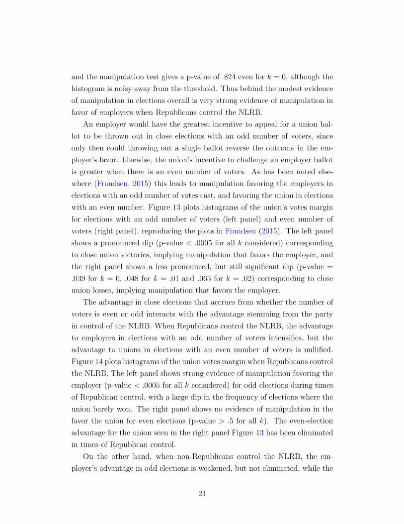
and the manipulation test gives a p-value of .824 even for k = 0, although the
histogram is noisy away from the threshold. Thus behind the modest evidence
of manipulation in elections overall is very strong evidence of manipulation in
favor of employers when Republicans control the NLRB.
An employer would have the greatest incentive to appeal for a union bal-
lot to be thrown out in close elections with an odd number of voters, since
only then could throwing out a single ballot reverse the outcome in the em-
ployer’s favor. Likewise, the union’s incentive to challenge an employer ballot
is greater when there is an even number of voters. As has been noted else-
where (Frandsen, 2015) this leads to manipulation favoring the employers in
elections with an odd number of votes cast, and favoring the union in elections
with an even number. Figure 13 plots histograms of the union’s votes margin
for elections with an odd number of voters (left panel) and even number of
voters (right panel), reproducing the plots in Frandsen (2015). The left panel
shows a pronounced dip (p-value < .0005 for all k considered) corresponding
to close union victories, implying manipulation that favors the employer, and
the right panel shows a less pronounced, but still significant dip (p-value =
.039 for k = 0, .048 for k = .01 and .063 for k = .02) corresponding to close
union losses, implying manipulation that favors the employer.
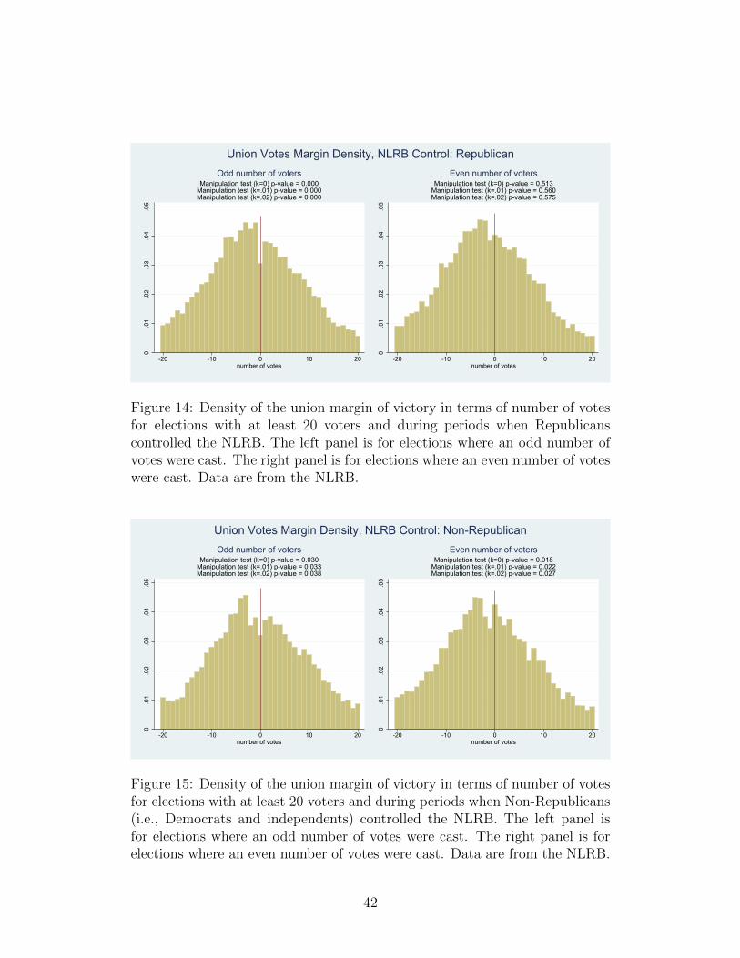
The advantage in close elections that accrues from whether the number of
voters is even or odd interacts with the advantage stemming from the party
in control of the NLRB. When Republicans control the NLRB, the advantage
to employers in elections with an odd number of voters intensifies, but the
advantage to unions in elections with an even number of voters is nullified.
Figure 14 plots histograms of the union votes margin when Republicans control
the NLRB. The left panel shows strong evidence of manipulation favoring the
employer (p-value < .0005 for all k considered) for odd elections during times
of Republican control, with a large dip in the frequency of elections where the
union barely won. The right panel shows no evidence of manipulation in the
favor the union for even elections (p-value > .5 for all k). The even-election
advantage for the union seen in the right panel Figure 13 has been eliminated
in times of Republican control.
On the other hand, when non-Republicans control the NLRB, the em-
ployer’s advantage in odd elections is weakened, but not eliminated, while the
21

union enjoys an even stronger advantage in even elections. Figure 15 plots his-
tograms of the union votes margin when non-Republicans control the NLRB.
The left panel shows evidence of manipulation in odd elections favoring the
employer (p-value = .03-.04) but to a lesser extent than when Republicans con-
trol the NLRB. The right panel shows strongest evidence yet of manipulation
in even elections favoring the union (p-value = .018-.027).
With additional assumptions, the magnitude as well as the presence of
manipulation can be estimated. Under the assumption that k = 0 and that
manipulation takes the form of disgarding unfavorable close elections, one can
estimate the fraction of “missing” elections at the threshold that would have
to be added back to result in a linear density. For example, the data suggest
that 21 percent of elections with an odd number of voters are “missing” from
the mass at the threshold (left panel, Figure 13).2
5 Conclusion
Many applications of the widely-used regression discontinuity design involve
running variables that are discrete. Discrete running variables pose special
problems in RD analysis that do not arise in the classical setup where the
running variable is continuously distributed, including specification and infer-
ence (Lee and Card, 2008). One such challenge is that frequently-used density
tests for manipulation in the running variable, such as McCrary (2008), are
inconsistent when the running variable is discretely distributed.
This paper proposed a test for manipulation that is consistent when the
running variable is discrete, and can also be used when the running variable
is continuously distributed. Monte Carlo simulations illustrated that the test
has correct size and good power even in settings where the smoothness approx-
imation near the threshold is not exact and through the range of parameters
relevant in practice. The same simulations also showed that tests designed for
a continuous variable will tend to falsely detect manipulation even when there
is none.
2There were 744 elections where the union was one vote shy of victory, and 675 wherethe union had one vote to spare. Assuming k = 0, one would expect (744 + 675) /2 = 709.5elections exactly at the threshold of union victory. Only 561 are observed, corresponding toa fraction missing of 1− 561/709.4 = .21.
22

Applying the test to NLRB union representation election outcomes revealed
strong evidence for manipulation in union elections. Overall the manipulation
appears to slightly favor the employer, but this overall slight advantage masks
large advantages to the employer when Republicans control the NLRB and ad-
vantages to the union otherwise. This evidence should sound a cautionary note
to reseachers on interpreting comparisons between establishments where the
union barely won or barely lost as reflecting the causal impact of unionization
and to policy makers, employers, and workers on the fairness and transparency
of the unionizing process.
Acknowledgment
The McCrary tests in the simulations were implemented using the Stata soft-
ware program DCdensity.ado available at http://emlab.berkeley.edu/ jmccrary/DCdensity/.
All default options were maintained except the binwidth of the discrete random
variable was specified.
The manipulation test for discrete running variables proposed in this paper
is available as a Stata command .ado file from the author upon request.
Appendix
Proofs
Proof of Theorem 1. By Bayes’ Rule,
Pr (R = 0|R ∈ {−∆, 0,∆}) =f (0)
f (−∆) + f (0) + f (∆). (1)
Rearranging the definition of a second-order finite difference allows us to write
f (0) =1
2(f (−∆) + f (∆))−∆(2)f (0) ∆2/2. (2)
Substituting for f (0) in equation (1) using equation (2) yields
Pr (R = 0|R ∈ {−∆, 0,∆}) =f (−∆) + f (∆)−∆(2)f (0) ∆2
3 (f (−∆) + f (∆))−∆(2)f (0) ∆2.
23

Since this expression is monotonic in ∆(2)f (0), bounds can be obtained by
substituting in the upper and lower bounds from Assumption 3, which yields
the theorem’s result.
Proof of Theorem 2. Under H0, the indicator 1 (Ri = 0) is by definition
conditionally Bernoulli with probability of success p ∈ P (k), conditional on
Ri ∈ {−∆, 0,∆}. Under the iid sampling assumed in the corollary’s premise,
then N0 consists of m conditionally independent draws of a Bernoulli random
variable, each with conditional probability of success p, and therefore is by
definition conditionally distributed as B (m, p).
Proof of Theorem 3. The minimization problem defining the critical values
always has at least one solution, since it involves minimization over a nonempty
finite set. The set is nonempty because the constraint is always satisfied over
some nontrivial subset (for example, CL = 0 and CU = m). The constraint
then implies the result, since by H0
Pr(CLα (k) < N0 < CU
a (k) |N−∆ +N0 +N∆ = m)
= Pr(N0 < CU
a (k) |N−∆ +N0 +N∆ = m)− Pr
(N0 ≤ CL
a (k) |N−∆ +N0 +N∆ = m)
≥ infp∈P(k)
FB(CU − 1,m, p
)− FB
(CL;m, p
)≥ 1− α,
where the first equality is by definition, the first inequality follows from The-
orem 2 and the definition of a cdf, and the final inequality follows from the
constraint.
Proof of Theorem 4. Note first that the probablity of rejection can be
written
Pr(N0/m ≤ CL
α (k) /m or N0/m ≥ CUα (k) /m|N−∆ +N0 +N∆ = m
).
Note that limn→∞CLα (k) /m = (1− k) / (3− k) and limn→∞C
Uα (k) /m =
(1 + k) / (3 + k). Note also that by the weak law of large numbers N0/m
converges in probability to (1− k) / (3− k)− δ or (1 + k) / (3 + k) + δ. Then
by the definition of convergence in probability
limn→∞
Pr(N0/m ≤ CL
α (k) /m or N0/m ≥ CUα (k) /m|N−∆ +N0 +N∆ = m
)= 1.
24
Linear Approximation Equivalency
This section shows formally that the result of Theorem 1 for the special case
of k = 0 is equivalent to a linear approximation in a fixed neighborhood of the
threshold. To be precise, consider the following definition of a linear pmf in a
neighborhood of the threshold:
Definition 1 (Linear probability mass function in a neighborhood of the threshold)
The probability mass function of R is linear in a neighborhood of rc if Pr (R = rc + r) =
Pr (R = rc) + δ (r − rc) for r ∈ {rc −∆, rc, rc + ∆}.
The key insight is that if R’s pmf is linear in a neighborhood of rc, then the
sample frequency at R = rc has the known conditional Bernoulli distribution
given in Theorem 1, and vice versa, as the following proposition shows.
Proposition 5 The probability mass function of R is linear in a neighborhood
of rc if and only if
Pr (R = rc|R ∈ {rc −∆, rc, rc + ∆}) = 1/3.
Proof. First the “only if” direction. By Bayes’ rule, Pr (R = rc|R ∈ {rc −∆, rc, rc + ∆})is
Pr (R = rc)
Pr (R = rc −∆) + Pr (R = rc) + Pr (R = rc + ∆).
By the defintion of a linear pmf in a neighborhood of rc, the denominator is
Pr (R = rc)−∆δ+Pr (R = rc)+Pr (R = rc)+∆δ = 3×Pr (R = rc). Now the
“if” direction. The result follows if Pr (R = rc|R ∈ {rc −∆, rc, rc + ∆}) = 1/3
implies that the difference in the conditional probability at R = rc + ∆ and
R = rc is equal to the difference in the conditional probability at R = rc and
R = rc −∆ (the difference would then be δ from the Definition). Start with
the difference between the conditional probability at R = rc + ∆ and R = rc.
25

By Bayes’ rule and the premise,
Pr (R = rc + ∆|R ∈ {rc −∆, rc, rc + ∆})− Pr (R = rc|R ∈ {rc −∆, rc, rc + ∆})
=Pr (R = rc + ∆)
Pr (R = rc −∆) + Pr (R = rc) + Pr (R = rc + ∆)− 1
3
= 1− Pr (R = rc −∆) + Pr (R = rc)
Pr (R = rc −∆) + Pr (R = rc) + Pr (R = rc + ∆)− 1
3
= 1−(
Pr (R = rc −∆)
Pr (R = rc −∆) + Pr (R = rc) + Pr (R = rc + ∆)+
1
3
)− 1
3
=1
3− Pr (R = rc −∆)
Pr (R = rc −∆) + Pr (R = rc) + Pr (R = rc + ∆)
= Pr (R = rc|R ∈ {rc −∆, rc, rc + ∆})− Pr (R = rc −∆|R ∈ {rc −∆, rc, rc + ∆}) .
Thus, the result of Theorem 1 for the case of k = 0 is equivalent to the
discrete running variable R having a linear pmf in a neighborhood of the
threshold.
References
Joshua D. Angrist and Victor Lavy. Using maimonides’ rule to estimate the
effect of class size on scholastic achievement. The Quarterly Journal of
Economics, 114(2):533–575, 1999.
Timothy B. Armstrong and Michal Kolesar. Optimal inference in a class of
regression models, 2015.
Dan Black, Jose Galdo, and Jeffrey Smith. Evaluating the bias of the regression
discontinuity design using experimental data. Mimeo, University of Chicago,
January 2007.
H. Buddelmeyer and E. Skoufias. An evaluation of the performance of regres-
sion discontinuity design on progresa. IZA, Bonn, Germany, 2003.
David Card and Lara D. Shore-Sheppard. Using discontinuous eligibility rules
to identify the effects of the federal medicaid expansions on low-income
children. The Review of Economics and Statistics, 86(3):pp. 752–766, 2004.
26
David Card, Carlos Dobkin, and Nicole Maestas. Does medicare save lives?
The Quarterly Journal of Economics, 124(2):pp. 597–636, 2009.
Matias D. Cattaneo, Michael Jansson, and Xinwei Ma. Simple local regression
distribution estimators with an application to manipulation testing. 2016.
Kenneth Y. Chay, Daeho Kim, and Shailender Swaminathan. Medicare, hos-
pital utilization and mortality: Evidence from the program’s origins. Un-
published manuscript, February 2010.
Thomas D. Cook and Vivian C. Wong. Empirical tests of the validity of the
regression-discontinuity design. Annales d’Economie et de Statistique, 2008.
forthcoming.
William N. Cooke and III Gautschi, Frederick H. Political bias in nlrb unfair
labor practice decisions. Industrial and Labor Relations Review, 35(4):pp.
539–549, 1982.
Stephen L. DesJardins, Brian P. McCall, Molly Ott, and Jiyun Kim. A quasi-
experimental investigation of how the gates millennium scholars program is
related to college students’ time use and activities. Educational Evaluation
and Policy Analysis, 32(4):pp. 456–475, 2010.
John DiNardo and David S. Lee. Economic impacts of new unionization on
private sector employers: 1984-2001. Quarterly Journal of Economics, 119
(4):1383–1441, 2004.
Yingying Dong. Regression discontinuity applications with rounding errors in
the running variable. Unpublished manuscript, 2012.
Brigham R. Frandsen. The surprising impacts of unionization on establish-
ments: Accounting for selection in close union representation elections. Un-
published manuscript, 2015.
Brigham R. Frandsen, Markus Frolich, and Blaise Melly. Quantile treatment
effects in the regression discontinuity design. Journal of Econometrics, 168
(2):382 – 395, 2012.
27
Pietro Garibaldi, Lia Pacelli, and Andrea Borgarello. Employment protec-
tion legislation and the size of firms. Giornale degli economisti e annali di
economia, pages 33–68, 2004.
Francois Gerard, Miikka Rokkanen, and Christoph Rothe. Partial identifica-
tion in regression discontinuity designs with manipulated running variables.
unpublished manuscript, August 2015.
William T. Gormley, Jr., Ted Gayer, Deborah Phillips, and Brittany Dawson.
The effects of universal pre-k on cognitive development. Developmental
Psychology, 41(6):872–884, 2005.
Jinyong Hahn, Petra Todd, and Wilbert van der Klaauw. Evaluating the
effect of an antidiscrimination law using a regression-discontinuity design.
Working Paper 7131, National Bureau of Economic Research, May 1999.
Jinyong Hahn, Petra Todd, and Wilbert van der Klaauw. Identification and es-
timation of treatment effects with a regression-discontinuity design. Econo-
metrica, 69(1):201–209, 2001.
Guido W. Imbens and Thomas Lemieux. Regression discontinuity designs: A
guide to practice. Journal of Econometrics, 142(2):615–635, 2008.
Darrell Issa. President obamas pro-union board: The nlrb’s metamorphosis
from independent regulator to dysfunctional union advocate. Staff Report,
U.S. House of Representatives 112th Congress Committee on Oversight and
Government Reform, December 2012.
Michal Kolesar and Christoph Rothe. Inference in regression discontinuity
designs with a discrete running variable. 2016.
David S. Lee. Randomized experiments from non-random selection in u.s.
house elections. Journal of Econometrics, 142(2):675 – 697, 2008. The
regression discontinuity design: Theory and applications.
David S. Lee and David Card. Regression discontinuity inference with speci-
fication error. Journal of Econometrics, 142(2):655 – 674, 2008.
28

David S. Lee and Thomas Lemieux. Regression discontinuity designs in eco-
nomics. Journal of Economic Literature, 48(2):281–355, September 2010.
David S. Lee and Alexandre Mas. Long-run impacts of unions on firms: New
evidence from financial markets, 1961-1999. The Quarterly Journal of Eco-
nomics, 127(1):333–378, 2012.
Chris J. Lloyd. Estimating test power adjusted for size. Journal of Statistical
Computation and Simulation, 75(11):921–933, 2005.
Jordan Matsudaira. Mandatory summer school and student achievement.
Journal of Econometrics, 142(2):829–850, 2008.
Justin McCrary. Manipulation of the running variable in the regression dis-
continuity design: A density test. Journal of Econometrics, 142:698–714,
2008.
Devin Pope and Uri Simonsohn. Round numbers as goals: Evidence from
baseball, sat takers, and the lab. Psychological Science, 22(1):pp. 71–79,
2011.
Jerome Sacks and Donald Ylvisaker. Linear estimation for approximately
linear models. Ann. Statist., 6(5):1122–1137, 09 1978.
Fabiano Schivardi and Roberto Torrini. Identifying the effects of firing restric-
tions through size-contingent differences in regulation. Labour Economics,
15(3):482–511, 2008.
Wilbert van der Klaauw. Regression discontinuity analysis: A survey of recent
developments in economics. LABOUR, 22(2):219–245, 2008.
Jane Waldfogel. The impact of the family and medical leave act. Journal of
Policy Analysis and Management, 18(2):281–302, 1999.
29
No manipulation: satisfies second finite-difference bound
Manipulation: violates second finite-difference bound
Figure 1: Example depicting an example where the second finite differencebound in Assumption 3 is satisfied (left panel) and where it is violated (rightpanel). The curves show the envelope for the probability mass function im-posed by the bound on the second-order finite difference.
30
McCrary (2008) test
Discrete test
0.2
.4.6
.81
0 2000 4000 6000 8000 10000sample size
k = 0.02 k = 0
Nominal size = .05Rejection rate by sample size
Figure 2: Monte Carlo simulation rejection rates from a McCrary (2008) test(dashed line) and the discrete test proposed in this paper (solid line) as afunction of the sample size (x-axis). The underlying distribution of the runningvariable is a discretized log-normal (no manipulation) with a bin width of .1,corresponding to a k parameter of .02. The nominal size of the tests is .05.Based on 1000 iterations.
31

McCrary (2008) test
Discrete test
0.0
5.1
.15
.2
0 .05 .1 .15 .2support point spacing
Nominal size = .05Rejection rate by Running Variable Coarseness
Figure 3: Monte Carlo simulation rejection rates from a McCrary (2008) test(dashed line) and the discrete test proposed in this paper (solid line) as afunction of the bin width of the discrete running variable. The underlying dis-tribution of the running variable is a discretized log-normal (no manipulation)with a bin width indicated on the x-axis. The nominal size of the tests is .05.Based on 1000 iterations with a sample size of 5,000 for each iteration.
32

McCrary (2008) test
Discrete test
0.2
.4.6
.8
0 2 4 6skewness
Nominal size = .05Rejection rate by skewness
Figure 4: Monte Carlo simulation rejection rates from a McCrary (2008) test(dashed line) and the discrete test proposed in this paper (solid line) as afunction of the skewness of the discrete running variable’s distribution. Theunderlying distribution of the running variable is a discretized log-normal (nomanipulation) with a binwidth of .1. The nominal size of the tests is .05.Based on 1000 iterations with a sample size of 3000 for each iteration.
33
0.5
11.
5D
ensi
ty
0 .5 1 1.5 2 2.5running variable
Simulated Running Variable with Manipulation
Figure 5: Simulated example of a discrete running variable with manipulationat the threshold.
34

McCrary (2008)test
Discrete test
McCrary (2008), size-adjusted
0.2
.4.6
.81
0 .2 .4 .6 .8 1Pr(manipulation at threshold)
Nominal size = .05Rejection rate by Degree of Manipulation
Figure 6: Monte Carlo simulation rejection rates from a McCrary (2008) test(unadjusted: long dashed line; adjusted: short dashed line) and the discretetest proposed in this paper (solid line) as a function of the degree of manip-ulation. The underlying distribution of the running variable is a discretized(binwidth = .1) log-normal but with a probability of switching to a pointabove the threshold for draws below the threshold, as described in the text.The maximum probability of switching (x-axis) occurs just below the thresh-old and fades exponentially at rate one moving away from the threshold. Thenominal size of the tests is .05. Based on 1000 iterations with a sample size of1,000 for each iteration.
35

0.2
.4.6
.81
0 .05 .1 .15 .2support point spacing
Pr(Manipulation at threshold) = .5Rejection rate by Running Variable Coarseness
Figure 7: Monte Carlo simulation rejection rates from the discrete test pro-posed in this paper as a function of the bin width of the discrete runningvariable. The underlying distribution of the running variable is a discretizedlog-normal but with a probability of switching to a point above the thresh-old for draws below the threshold, as described in the text. The maximumprobability of switching is .5 and occurs just below the threshold and fadesexponentially at rate one moving away from the threshold. The nominal sizeof the tests is .05. Based on 1000 iterations with a sample size of 5,000 foreach iteration.
36
0.2
.4.6
.81
0 .1 .2 .3 .4 .5support point spacing
Nominal size = .05
Pushing the Approximation:Rejection rate by Running Variable Coarseness
Figure 8: Monte Carlo simulation rejection rates from the discrete test pro-posed in this paper as a function of the bin width of the discrete runningvariable. The underlying distribution of the running variable is a discretizedlog-normal (no manipulation) with a bin width indicated on the x-axis. Thenominal size of the tests is .05. Based on 1000 iterations with a sample size of5,000 for each iteration.
37
0.2
.4.6
.81
0 .05 .1 .15 .2k
Power by Degree of Curvature Allowed
Figure 9: Monte Carlo simulation rejection rates from the discrete test pro-posed in this paper as a function of the choice of k. The underlying distributionof the running variable is a discretized log-normal but with a probability ofswitching to a point above the threshold for draws below the threshold, asdescribed in the text. The maximum probability of switching is .4 and occursjust below the threshold and fades exponentially at rate one moving away fromthe threshold. The nominal size of the tests is .05. Based on 1000 iterationswith a sample size of 1,000 for each iteration.
38
Non
−R
epub
lican
Rep
ublic
an
1980q1 1990q1 2000q1 2010q1Election date
Party in Control of NLRB, 1980 − 2009
Figure 10: Reproduced from Frandsen (2015). The top series indicates theperiods when Republicans held a majority of the NLRB seats and the bot-tom series indicates the periods when Non-Republicans (i.e., Democrats orindependents) held a majority. Data are from the NLRB.
39

0.0
1.0
2.0
3.0
4.0
5
-20 -10 0 10 20number of votes
Manipulation test (k=0) p-value = 0.077Manipulation test (k=.01) p-value = 0.092Manipulation test (k=.02) p-value = 0.133
Union Votes Margin Density
Figure 11: Density of the union margin of victory in terms of number of votesfor elections with at least 20 voters. Data are from the NLRB. Histogramreproduced from Frandsen (2015).
40

0.0
1.0
2.0
3.0
4.0
5
-20 -10 0 10 20number of votes
Manipulation test (k=0) p-value = 0.010Manipulation test (k=.01) p-value = 0.011Manipulation test (k=.02) p-value = 0.017
NLRB Control: Republican
0.0
1.0
2.0
3.0
4.0
5
-20 -10 0 10 20number of votes
Manipulation test (k=0) p-value = 0.824Manipulation test (k=.01) p-value = 0.867Manipulation test (k=.02) p-value = 0.876
NLRB Control: Non-Republican
Union Votes Margin Density
Figure 12: Density of the union margin of victory in terms of number of votesfor elections with at least 20 voters. The left panel is for elections held duringperiods when Republicans controlled the NLRB. The right panel is for electionsheld during periods when Non-Republicans (i.e., Democrats and independents)controlled the NLRB. Data are from the NLRB. Histogram reproduced fromFrandsen (2015).
0.0
1.0
2.0
3.0
4.0
5
-20 -10 0 10 20number of votes
Manipulation test (k=0) p-value = 0.000Manipulation test (k=.01) p-value = 0.000Manipulation test (k=.02) p-value = 0.000
Odd number of voters
0.0
1.0
2.0
3.0
4.0
5
-20 -10 0 10 20number of votes
Manipulation test (k=0) p-value = 0.039Manipulation test (k=.01) p-value = 0.048Manipulation test (k=.02) p-value = 0.063
Even number of voters
Union Votes Margin Density
Figure 13: Density of the union margin of victory in terms of number of votesfor elections with at least 20 voters. The left panel is for elections where anodd number of votes were cast. The right panel is for elections where an evennumber of votes were cast. Data are from the NLRB.
41
0.0
1.0
2.0
3.0
4.0
5
-20 -10 0 10 20number of votes
Manipulation test (k=0) p-value = 0.000Manipulation test (k=.01) p-value = 0.000Manipulation test (k=.02) p-value = 0.000
Odd number of voters
0.0
1.0
2.0
3.0
4.0
5
-20 -10 0 10 20number of votes
Manipulation test (k=0) p-value = 0.513Manipulation test (k=.01) p-value = 0.560Manipulation test (k=.02) p-value = 0.575
Even number of voters
Union Votes Margin Density, NLRB Control: Republican
Figure 14: Density of the union margin of victory in terms of number of votesfor elections with at least 20 voters and during periods when Republicanscontrolled the NLRB. The left panel is for elections where an odd number ofvotes were cast. The right panel is for elections where an even number of voteswere cast. Data are from the NLRB.
0.0
1.0
2.0
3.0
4.0
5
-20 -10 0 10 20number of votes
Manipulation test (k=0) p-value = 0.030Manipulation test (k=.01) p-value = 0.033Manipulation test (k=.02) p-value = 0.038
Odd number of voters
0.0
1.0
2.0
3.0
4.0
5
-20 -10 0 10 20number of votes
Manipulation test (k=0) p-value = 0.018Manipulation test (k=.01) p-value = 0.022Manipulation test (k=.02) p-value = 0.027
Even number of voters
Union Votes Margin Density, NLRB Control: Non-Republican
Figure 15: Density of the union margin of victory in terms of number of votesfor elections with at least 20 voters and during periods when Non-Republicans(i.e., Democrats and independents) controlled the NLRB. The left panel isfor elections where an odd number of votes were cast. The right panel is forelections where an even number of votes were cast. Data are from the NLRB.
42


