Download - Partitioning and Divide-and-Conquer Strategies Cluster Computing, UNC-Charlotte, B. Wilkinson, 2007
Partitioning and Divide-and-Conquer Strategies
Cluster Computing, UNC-Charlotte, B. Wilkinson, 2007.

4.1
Partitioning
Partitioning simply divides the problem into parts and then compute the parts and combine results.
1. data partition or domain partition: divide the data and operate upon the divided data concurrently.
2. functional decomposing: divide into independent functions and execute them concurrently.

4.1
Divide and Conquer
Characterized by dividing problem into sub-problems of same. Further divisions into still smaller sub-problems, usually done by recursion.
Recursive divide and conquer amenable to parallelization because separate processes can be used for divided parts. Also usually data is naturally localized.

4.2
Partitioning/Divide and Conquer Examples
Many possibilities.
• Operations on sequences of number such as simply adding them together
• Several sorting algorithms can often be partitioned or constructed in a recursive fashion
• Numerical integration
• N-body problem

4.3
Partitioning a sequence of numbers into parts and adding the parts

• Possible parallel programs:• 1. Numbers are sent from the master to the
slaves. Master will only send the specific numbers to the slaves. Slaves do the summation and send the results back.
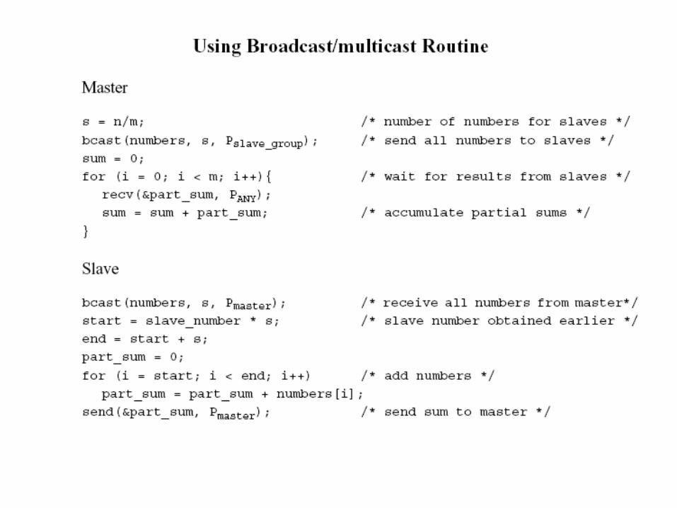
• 2. Master broadcasts the whole list to slaves. The specifics of the broadcast mechanism would need to be known in order to decide the merits. Usually, a broadcast will have a single startup time rather than separate startup times.
• 3. Use scatter and reduce.


• Speedup factor:
Computation and communication ratio:
( 1)
(2 ( ) 2)
( 2)
(2 ( ) )
startup data
startup data
nn
mt n m t mm
nm
mmt n m t

Problems Seen • Speedup factor is low if small n and large
m because the slaves are idle during the fourth phase.
• Ideally, we want all the processes to be active all of the time, which cannot be achieved by this formulation of problem.
• So what strategy is better??
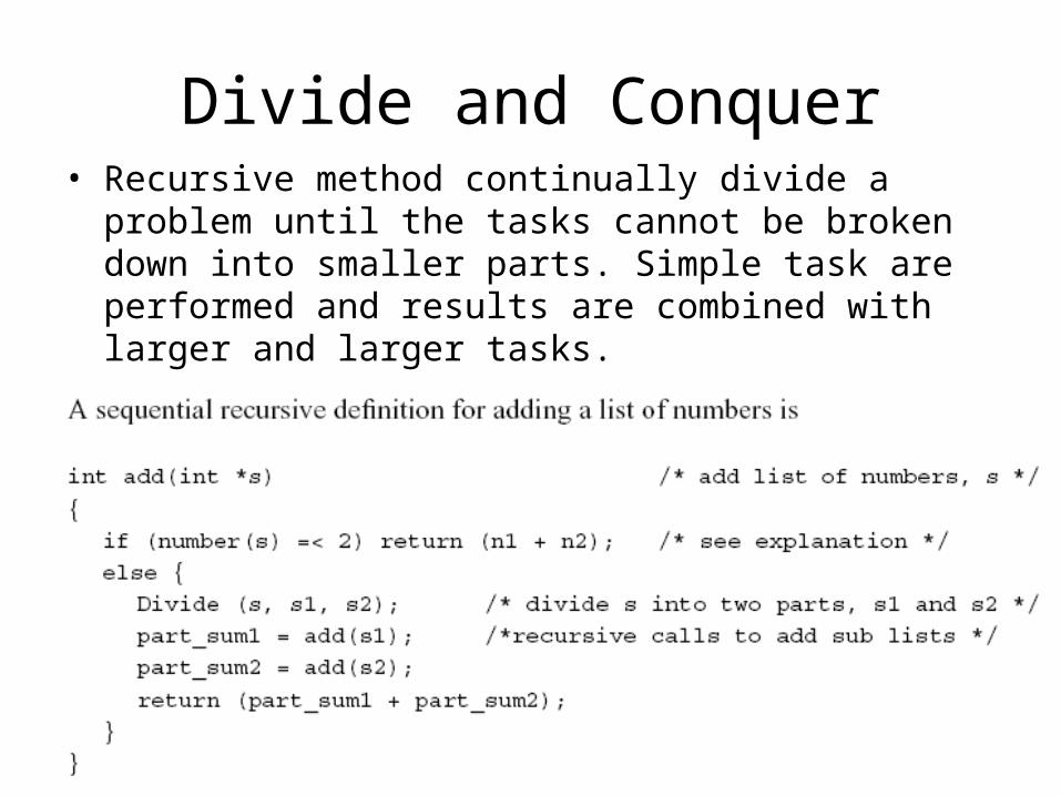
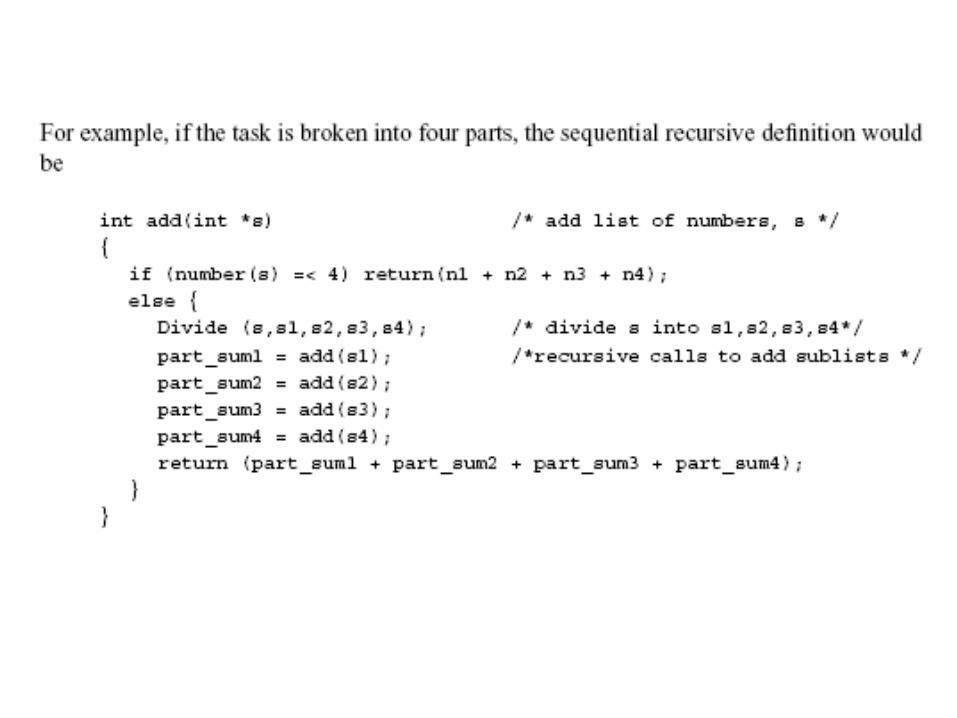
Divide and Conquer• Recursive method continually divide a problem until the
tasks cannot be broken down into smaller parts. Simple task are performed and results are combined with larger and larger tasks.
• A recursive formulation:

4.4
Tree construction
A well balanced tree is created. We can assign each node a separate processor . We will need 2^k -1 processors, where k is the total level number

4.5
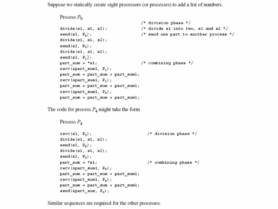
Dividing a list into parts

4.6
Partial summation
Divide and Conquer
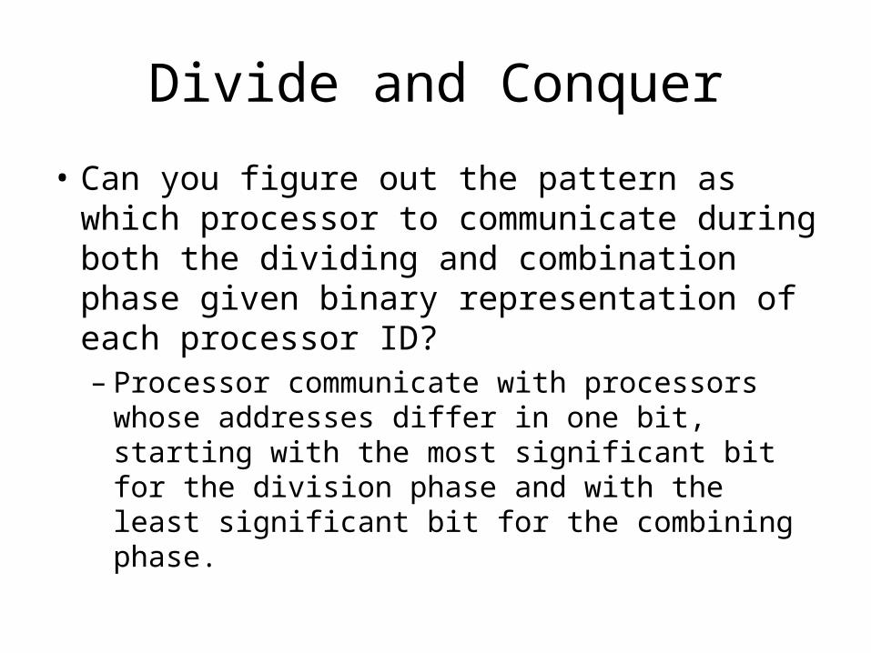
• Can you figure out the pattern as which processor to communicate during both the dividing and combination phase given binary representation of each processor ID?– Processor communicate with processors whose
addresses differ in one bit, starting with the most significant bit for the division phase and with the least significant bit for the combining phase.
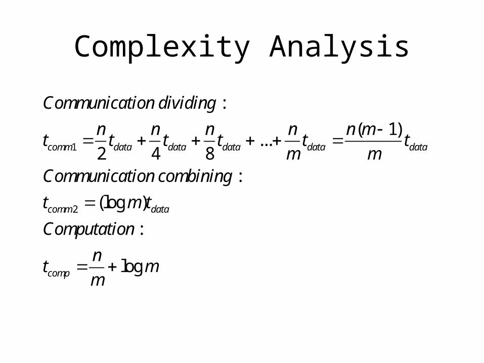
Complexity Analysis
1
2
:
( 1)...
2 4 8:
(log )
:
log
comm data data data data data
comm data
comp
Communication dividing
n n n n n mt t t t t t
m mCommunication combining
t m t
Computation
nt m
m

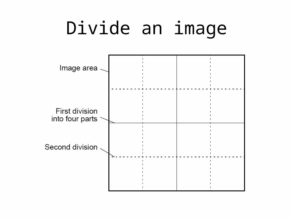
M-ary Divide and Conquer
• A task is divided into more than two parts at each stage. Achieve a higher level of parallel processing.
• For example, a tree can have four children at each node.
• A digitized image could be divided into four quadrants and each of the four quadrants divided into four subquadrants and so on.
• An octtree is a tree in which each node has eight children. It is used in three dimension dataset.

Quadtree
Divide an image

Octree
Image from wiki

Numerical Integration
• Computing the “area under the curve.”
• Parallelized by divided area into smaller areas (partitioning).
• Can also apply divide and conquer -- repeatedly divide the areas recursively.

Numerical Integration
4.15
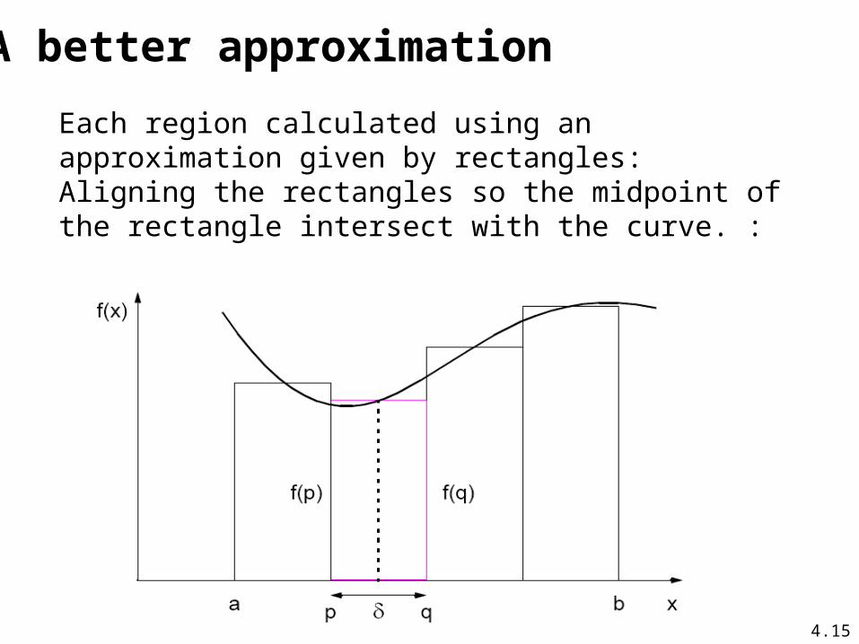
A better approximation
Each region calculated using an approximation given by rectangles:Aligning the rectangles so the midpoint of the rectangle intersect with the curve. :

4.16
Numerical integration using trapezoidal method
Trapezoid is a quadrilateral

Static Assignment

4.17
Adaptive QuadratureNumber of intervals is fixed. However, we could increase the number of intervals until two rounds of computation give similar results. We can keep doubling the number of interval until computation converges. Solution adapts to shape of curve. Use three areas, A, B, and C. Computation terminated when largest of A and B sufficiently close to sum of remain two areas .
4.18
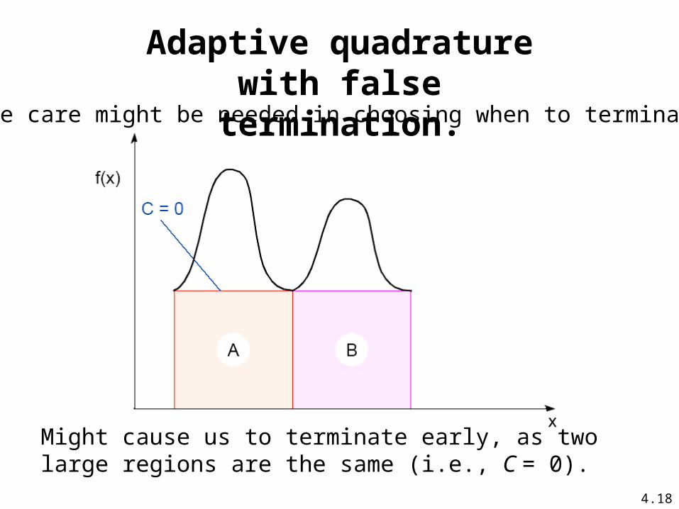
Adaptive quadrature with false termination.
Some care might be needed in choosing when to terminate.
Might cause us to terminate early, as two large regions are the same (i.e., C = 0).

4.25
Gravitational N-Body Problem
Finding positions and movements of bodies in space subject to gravitational forces from other bodies, using Newtonian laws of physics.
4.26
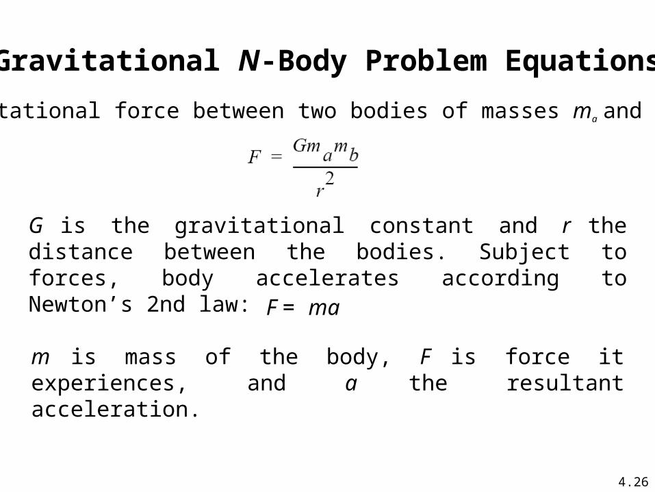
Gravitational N-Body Problem Equations
Gravitational force between two bodies of masses ma and mb is:
G is the gravitational constant and r the distance between the bodies. Subject to forces, body accelerates according to Newton’s 2nd law:
m is mass of the body, F is force it experiences, and a the resultant acceleration.
F = ma
4.27
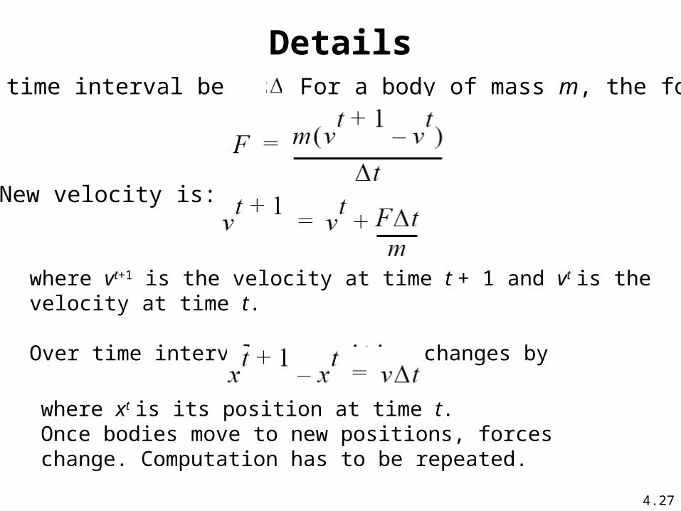
New velocity is:
where vt+1 is the velocity at time t + 1 and vt is the velocity at time t.
Over time interval t, position changes by
where xt is its position at time t.Once bodies move to new positions, forces change. Computation has to be repeated.
DetailsLet the time interval be t. For a body of mass m, the force is:


3.28
Sequential Code
Overall gravitational N-body computation can be described by:
for (t = 0; t < tmax; t++) /* for each time period */for (i = 0; i < N; i++) { /* for each body */ F = Force_routine(i); /* compute force on ith body */
v[i]new = v[i] + F * dt / m; /* compute new velocity */ x[i]new = x[i] + v[i]new * dt; /* and new position */
}for (i = 0; i < N; i++) { /* for each body */ x[i] = x[i]new; /* update velocity & position*/ v[i] = v[i]new;}

4.29
Parallel Code
The sequential algorithm is an O(N2) algorithm (for one iteration) as each of the N bodies is influenced by each of the other N - 1 bodies.
Not feasible to use this direct algorithm for most interesting N-body problems where N is very large.

4.30
Time complexity can be reduced approximating a cluster of distant bodies as a single distant body with mass sited at the center of mass of the cluster:M =sum (mi); and C = 1/M * sum(mi * ci)

4.31
Barnes-Hut AlgorithmStart with whole space in which one cube contains the bodies (or particles).
• First, this cube is divided into four subcubes.
• If a subcube contains no particles, subcube deleted from further consideration.
• If a subcube contains one body, subcube retained.
• If a subcube contains more than one body, it is recursively divided until every subcube contains one body.

4.34
Recursive division of 2-dimensional space
Barnes-Hut Algorithm
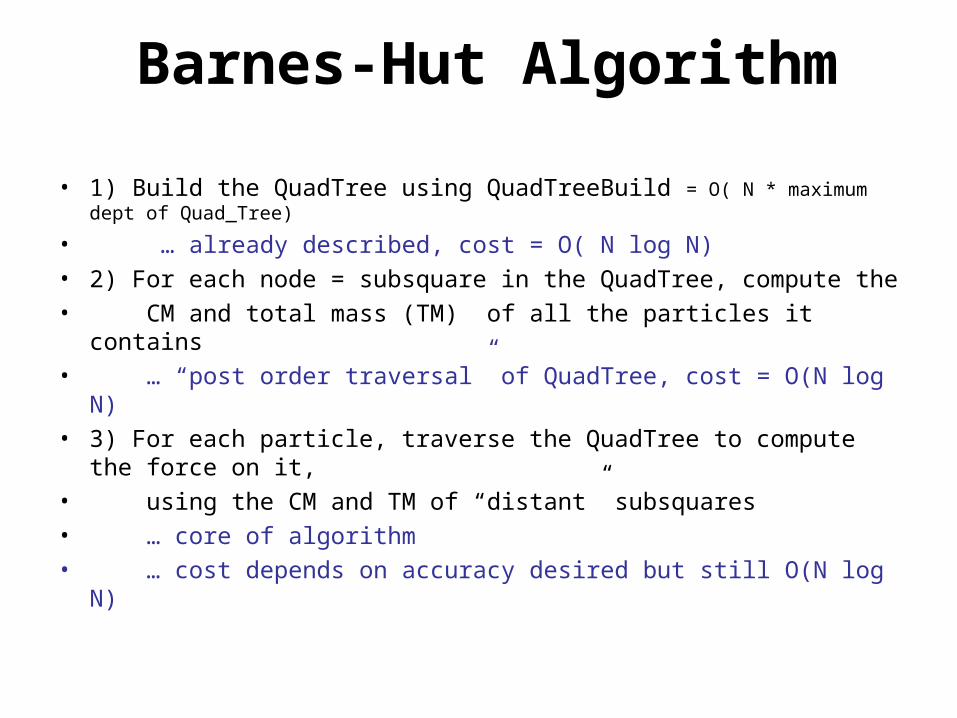
• 1) Build the QuadTree using QuadTreeBuild = O( N * maximum dept of Quad_Tree)
• … already described, cost = O( N log N)• 2) For each node = subsquare in the QuadTree, compute the • CM and total mass (TM) of all the particles it contains• … “post order traversal” of QuadTree, cost = O(N log N)• 3) For each particle, traverse the QuadTree to compute the force on
it, • using the CM and TM of “distant” subsquares• … core of algorithm • … cost depends on accuracy desired but still O(N log N)
4.32
Creates an octtree - a tree with up to eight edges from each node.
The leaves represent cells each containing one body.
After the tree has been constructed, the total mass and center of mass of the subcube is stored at each node.
4.33
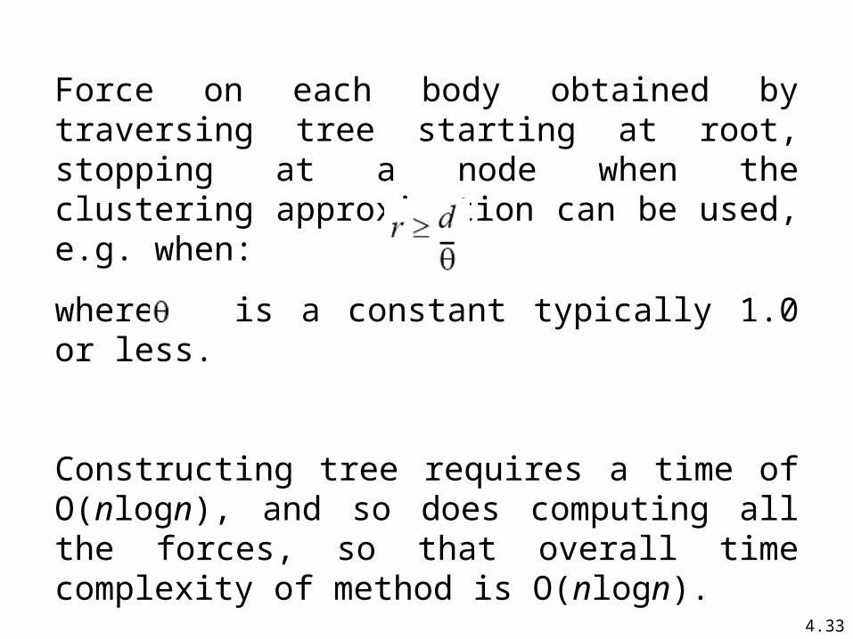
Force on each body obtained by traversing tree starting at root, stopping at a node when the clustering approximation can be used, e.g. when:
where is a constant typically 1.0 or less.
Constructing tree requires a time of O(nlogn), and so does computing all the forces, so that overall time complexity of method is O(nlogn).

4.35
(For 2-dimensional area) First, a vertical line found that divides area into two areas each with equal number of bodies. For each area, a horizontal line found that divides it into two areas each with equal number of bodies. Repeated as required.
Orthogonal Recursive Bisection

4.36
Astrophysical N-body simulationBy Scott Linssen (UNCC student, 1997) using O(N2) algorithm.
4.37
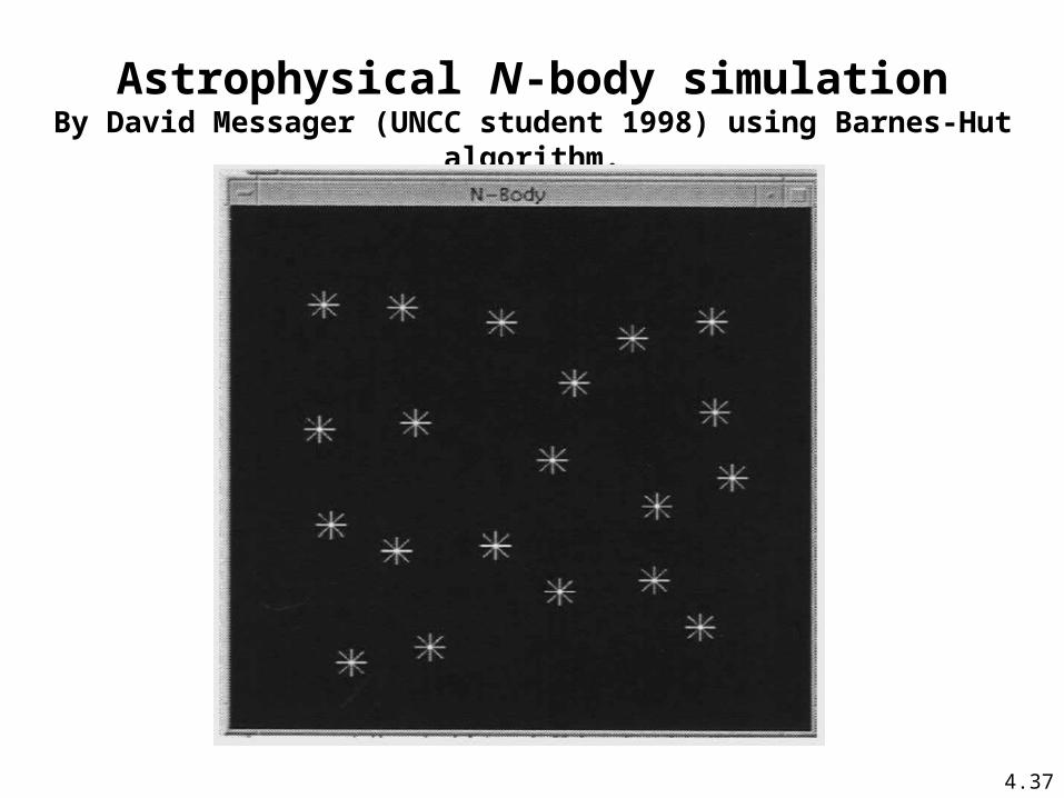
Astrophysical N-body simulationBy David Messager (UNCC student 1998) using Barnes-Hut algorithm.
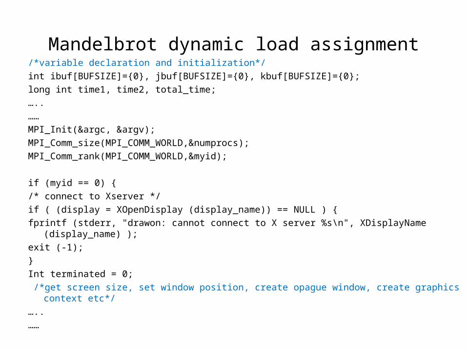
Mandelbrot dynamic load assignment/*variable declaration and initialization*/
int ibuf[BUFSIZE]={0}, jbuf[BUFSIZE]={0}, kbuf[BUFSIZE]={0};
long int time1, time2, total_time;
…..
……
MPI_Init(&argc, &argv);
MPI_Comm_size(MPI_COMM_WORLD,&numprocs);
MPI_Comm_rank(MPI_COMM_WORLD,&myid);
if (myid == 0) {
/* connect to Xserver */
if ( (display = XOpenDisplay (display_name)) == NULL ) {
fprintf (stderr, "drawon: cannot connect to X server %s\n", XDisplayName (display_name) );
exit (-1);
}
Int terminated = 0;
/*get screen size, set window position, create opague window, create graphics context etc*/
…..
……

while( !terminated) {
for(id = 1; id < numprocs; id++) { // Check for any messages waiting to be received
MPI_Iprobe(id, 0, MPI_COMM_WORLD, &flag, &status);
if(flag == 1) { // If you find one, receive it
MPI_Recv(&ibuf, bufsize, MPI_INT, id, 0, MPI_COMM_WORLD, &status);
MPI_Recv(&jbuf, bufsize, MPI_INT, id, 1, MPI_COMM_WORLD, &status);
MPI_Recv(&kbuf, bufsize, MPI_INT, id, 2, MPI_COMM_WORLD, &status);
/*draw points*/
XSetForeground (display, gc, kbuf[i]);
XDrawPoint (display, win, gc, jbuf[i], ibuf[i]);
// Search for next available task, If a task is found, Send the task say row number with data_tag to be 1 to slave with id
MPI_Send(&row, 1, MPI_INT, id, 1, MPI_COMM_WORLD);
}
//If NO task is marked Available or Busy then all tasks are DONE
terminated= 1;
}
Master node keeps check result, receive and send task
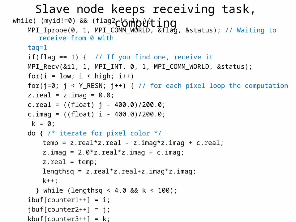
while( (myid!=0) && (flag2 != 1) ){
MPI_Iprobe(0, 1, MPI_COMM_WORLD, &flag, &status); // Waiting to receive from 0 with
tag=1
if(flag == 1) { // If you find one, receive it
MPI_Recv(&i1, 1, MPI_INT, 0, 1, MPI_COMM_WORLD, &status);
for(i = low; i < high; i++)
for(j=0; j < Y_RESN; j++) { // for each pixel loop the computation
z.real = z.imag = 0.0;
c.real = ((float) j - 400.0)/200.0;
c.imag = ((float) i - 400.0)/200.0;
k = 0;
do { /* iterate for pixel color */
temp = z.real*z.real - z.imag*z.imag + c.real;
z.imag = 2.0*z.real*z.imag + c.imag;
z.real = temp;
lengthsq = z.real*z.real+z.imag*z.imag;
k++;
} while (lengthsq < 4.0 && k < 100);
ibuf[counter1++] = i;
jbuf[counter2++] = j;
kbuf[counter3++] = k;
} // match for loop
Slave node keeps receiving task, computing

Slave node keeps receiving task, computing continues
MPI_Send(&ibuf, bufsize, MPI_INT, 0, 0, MPI_COMM_WORLD);
// sending x-coords
MPI_Send(&jbuf, bufsize, MPI_INT, 0, 1, MPI_COMM_WORLD);
// sending y-coords
MPI_Send(&kbuf, bufsize, MPI_INT, 0, 2, MPI_COMM_WORLD);
// sending color
} //match if (flag==1)
MPI_Iprobe(0, 3, MPI_COMM_WORLD, &flag2, &status); // check if master sends termination with data_tag to be 3
if( flag2 == 1 ) // termination received, slave should stop probing by flag2==1
MPI_Recv(&i1, 1, MPI_INT, 0, 3, MPI_COMM_WORLD, &status);
}
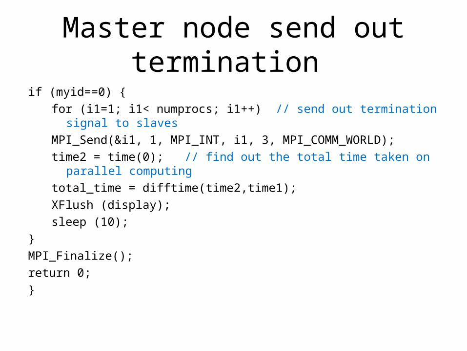
Master node send out termination
if (myid==0) {
for (i1=1; i1< numprocs; i1++) // send out termination signal to slaves
MPI_Send(&i1, 1, MPI_INT, i1, 3, MPI_COMM_WORLD);
time2 = time(0); // find out the total time taken on parallel computing
total_time = difftime(time2,time1);
XFlush (display);
sleep (10);
}
MPI_Finalize();
return 0;
}


