
Development of Improved Procedures for Seismic Design of Buried and Partially Buried Structures
Linda Al Atik
and
Nicholas Sitar
Department of Civil and Environmental EngineeringUniversity of California, Berkeley
Final report on research supported by the San Francisco Bay Area Rapid Transit (BART) and the Santa Clara Valley Transportation Authority (VTA)
PEER 2007/06JUne 2007
PACIFIC EARTHQUAKE ENGINEERING RESEARCH CENTER

Development of Improved Procedures for Seismic Design of Buried and
Partially Buried Structures
by
Linda Al Atik and Nicholas Sitar Department of Civil and Environmental Engineering
University of California, Berkeley
Final report on research supported by the San Francisco Bay Area Rapid Transit (BART) and the Santa Clara Valley Transportation Authority (VTA)
PEER Report 2007/06 Pacific Earthquake Engineering Research Center
College of Engineering University of California, Berkeley
June 2007

iii
ABSTRACT
Two sets of dynamic centrifuge model experiments were performed to evaluate the magnitude
and distribution of seismically induced lateral earth pressures on retaining structures that are
representative of designs currently under consideration by the Bay Area Rapid Transit (BART)
and the Valley Transportation Authority (VTA). Two U-shaped cantilever retaining structures,
one flexible and one stiff, were used to model the prototype structures, and dry medium-dense
sand at 61% and 72% relative density was used as backfill.
The results of the centrifuge experiments show that the maximum dynamic earth pressure
increases with depth and can be reasonably approximated by a triangular distribution analogous
to that used to represent static earth pressure. In general, the magnitude of the seismic earth
pressure depends on the magnitude and intensity of shaking, the density of the backfill soil, and
the flexibility of the retaining walls. The resulting relationship between the seismic earth
pressure coefficient increment (!KAE) and PGA suggests that seismic earth pressures can be
neglected at accelerations below 0.3 g. This is consistent with the observations and analyses
performed by Clough and Fragaszy (1977) and Fragaszy and Clough (1980), who concluded that
conventionally designed cantilever walls with granular backfill could reasonably be expected to
resist seismic loads at accelerations up to 0.5 g.
Conventional seismic design procedures based on the Mononobe and Okabe work that
are currently in use were found to provide conservative estimates of the seismic earth pressures
and the resulting dynamic moments. Specifically, the BART design criterion for rigid walls
appears amply conservative, especially if the normal factors of safety are taken into account. The
BART design criterion for flexible walls appears to be somewhat unconservative for loose
backfill. However, considering the various factors of safety present in the conventional design it
may in fact contain an appropriate level of conservatism.
An important contribution to the overall moment acting on the wall is the mass of the
wall itself. The data from the centrifuge experiments suggest that this contribution may be as
much as 25%. Given that the conventional analyses methods tend to give adequately
conservative results without the separate consideration of the wall inertial effects, the
contribution of seismic earth pressures to the overall moment acting on the retaining structures is
apparently routinely overestimated. Further analyses are needed to fully evaluate the impact of
this observation on the overall design.

iv
ACKNOWLEDGMENTS
This research was supported by the San Francisco Bay Area Rapid Transit (BART) and the Santa
Clara Valley Transportation Authority (VTA), through the Pacific Earthquake Engineering
Research Center (PEER). This work made use of the Earthquake Engineering Research Centers
Shared Facilities supported by the National Science Foundation under award number EEC-
9701568 through PEER. Any opinions, findings, and conclusions or recommendations expressed
in this material are those of the authors and do not necessarily reflect those of the funding
agencies.
The authors gratefully acknowledge the support and technical input provided by Mr. Ed
Matsuda and Dr. Jose Vallenas at BART and Mr. James Chai at VTA. The authors also received
much valuable input from Mr. John Egan at Geomatrix, Mr. Tom Boardman at Kleinfelder, Dr.
Marshall Lew at MACTEC, and Prof. Jonathan Bray at UC Berkeley. Professor Bruce Kutter,
Dr. Dan Wilson and all the staff at the Center for Geotechnical Modeling at the University of
California, Davis, provided much support and valuable input during the experimental phase of
this study.

v
CONTENTS
ABSTRACT.................................................................................................................................. iii
ACKNOWLEDGMENTS ........................................................................................................... iv
TABLE OF CONTENTS ..............................................................................................................v
LIST OF FIGURES .................................................................................................................... vii
LIST OF TABLES .................................................................................................................... xvii
1 BACKGROUND....................................................................................................................1
1.1 Dynamic Geotechnical Centrifuge Testing.....................................................................2
1.2 Scaling Relationships ......................................................................................................3
1.3 Literature Review............................................................................................................3
1.3.1 Analytical Methods .............................................................................................4
1.3.2 Numerical Methods.............................................................................................7
1.3.3 Experimental Studies ..........................................................................................8
2 EXPERIMENTAL SETUP.................................................................................................11
2.1 UC Davis Centrifuge, Shake Table, and Model Container...........................................11
2.2 Models Configuration ...................................................................................................12
2.3 Soil Properties ...............................................................................................................14
2.4 Structures Properties .....................................................................................................14
2.5 Model Preparation.........................................................................................................15
2.6 Instrumentation .............................................................................................................18
2.7 Calibration.....................................................................................................................20
2.8 Shaking Events..............................................................................................................21
2.9 Limitations ....................................................................................................................27
3 EXPERIMENTAL RESULTS ...........................................................................................29
3.1 Acceleration Response and Ground Motion Parameters ..............................................29
3.2 Soil Settlement and Densification.................................................................................49
3.3 Shear Wave Velocity ....................................................................................................50
3.4 Moment Distributions ...................................................................................................52
3.4.1 Analysis Procedure and Assumptions...............................................................52
3.4.2 Results: Time Series..........................................................................................54

vi
3.4.3 Static Moments .................................................................................................55
3.4.4 Total Dynamic Moments...................................................................................61
3.4.5 Dynamic Moment Increments...........................................................................71
3.5 Shear Distributions........................................................................................................82
3.5.1 Analysis Procedure and Assumptions...............................................................82
3.5.2 Total Dynamic Shear Distributions...................................................................83
3.6 Lateral Earth Pressures..................................................................................................93
3.6.1 Analysis Procedure and Assumptions...............................................................93
3.6.2 Total Dynamic Earth Pressures.........................................................................94
3.7 Performance: Total Dynamic Moment Time Histories...............................................109
3.8 Performance: Dynamic Moment Increment Time Histories.......................................125
3.9 Dynamic Active Earth Pressure Coefficients..............................................................141
3.10 Wall Inertial Effects on Moment and Pressure Distributions .....................................146
3.11 Wall Deflections .........................................................................................................150
4 CONCLUSIONS AND RECOMMENDATIONS ..........................................................155
4.1 Overview.....................................................................................................................155
4.2 Conclusions.................................................................................................................156
4.2.1 Seismic Earth Pressure Distribution................................................................156
4.2.2 Seismic Earth Pressure Magnitude..................................................................157
4.2.3 Dynamic Moments on Walls...........................................................................158
4.2.4 Effective Duration of Loading ........................................................................159
4.3 Limitations and Recommendations for Future Work..................................................159
REFERENCES...........................................................................................................................161
APPENDIX: TABLES...............................................................................................................165
vii
LIST OF FIGURES
Fig. 1.1 Forces considered in Mononobe-Okabe analysis (Wood 1973) .....................................5
Fig. 1.2 Wood (1973) rigid problem ............................................................................................7
Fig. 2.1 Model container FSB2 ..................................................................................................12
Fig. 2.2 LAA01 model configuration, profile view....................................................................13
Fig. 2.3 LAA02 model configuration, profile view....................................................................13
Fig. 2.4 Stiff and flexible model structures configuration (dimensions: in.)..............................15
Fig. 2.5 Pluviation of sand inside model container ....................................................................16
Fig. 2.6 Leveling sand surface with a vacuum ...........................................................................16
Fig. 2.7 Model under construction..............................................................................................17
Fig. 2.8 Model on centrifuge arm ...............................................................................................17
Fig. 2.9 Flexiforce, strain gages, and force-sensing bolts on south stiff wall during
experiment LAA02........................................................................................................19
Fig. 2.10 Flexiforce, strain gages, force-sensing bolts layout on south stiff and north flexible
walls for LAA01............................................................................................................19
Fig. 2.11 Flexiforce, strain gages, force-sensing bolts layout on south stiff and north flexible
walls for LAA02............................................................................................................20
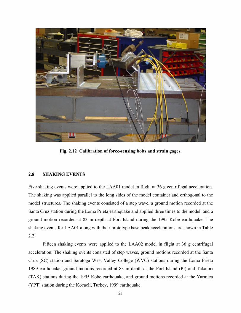
Fig. 2.12 Calibration of force-sensing bolts and strain gages.......................................................21
Fig. 2.13 Comparison of original Loma Prieta-SC090 source record to input Loma Prieta-
SC-1, LAA02 record and their response spectra ...........................................................23
Fig. 2.14 Comparison of original Kobe-TAK090 source record to input Kobe-TAK090-2,
LAA02 record and their response spectra .....................................................................24
Fig. 2.15 Comparison of original Koaceli-YPT060 source record to input Kocaeli-
YPT060-2, LAA02 record and their response spectra ..................................................25
Fig. 2.16 Comparison of original Loma Prieta-WVC270 source record to input Loma Prieta-
WVC270-1, LAA02 record and their response spectra ................................................26
Fig. 3.1 Horizontal acceleration, velocity, displacement, Arias intensity and response
spectrum of Loma Prieta-1 input motion for LAA01....................................................31
Fig. 3.2 Horizontal acceleration, velocity, displacement, Arias intensity and response
spectrum of Loma Prieta-2 input motion for LAA01....................................................32

viii
Fig. 3.3 Horizontal acceleration, velocity, displacement, Arias intensity, and response
spectrum of Kobe input motion for LAA01..................................................................33
Fig. 3.4 Horizontal acceleration, velocity, displacement, Arias intensity, and response
spectrum of Loma Prieta-3 input motion for LAA01....................................................34
Fig. 3.5 Horizontal acceleration, velocity, displacement, Arias intensity, and response
spectrum of Loma Prieta-SC-1 input motion during LAA02........................................35
Fig. 3.6 Horizontal acceleration, velocity, displacement, Arias intensity, and response
spectrum of Kobe-PI-1 input motion during LAA02....................................................36
Fig. 3.7 Horizontal acceleration, velocity, displacement, Arias intensity, and response
spectrum of Kobe-PI-2 input motion during LAA02....................................................37
Fig. 3.8 Horizontal acceleration, velocity, displacement, Arias intensity, and response
spectrum of Loma Prieta-SC-2 input motion during LAA02........................................38
Fig. 3.9 Horizontal acceleration, velocity, displacement, Arias intensity, and response
spectrum of the Kocaeli-YPT060-1 input motion during LAA02 ................................39
Fig. 3.10 Horizontal acceleration, velocity, displacement, Arias intensity, and response
spectrum of the Kocaeli-YPT060-2 input motion during LAA02 ................................40
Fig. 3.11 Horizontal acceleration, velocity, displacement, Arias intensity, and response
spectrum of the Kocaeli-YPT060-3 input motion during LAA02 ................................41
Fig. 3.12 Horizontal acceleration, velocity, displacement, Arias intensity and response
spectrum of Kocaeli-YPT330-1 input motion during LAA02 ......................................42
Fig. 3.13 Horizontal acceleration, velocity, displacement, Arias intensity, and response
spectrum of Kocaeli-YPT330-2 input motion during LAA02 ......................................43
Fig. 3.14 Horizontal acceleration, velocity, displacement, Arias intensity, and response
spectrum of Kobe-TAK090-1 input motion during LAA02 .........................................44
Fig. 3.15 Horizontal acceleration, velocity, displacement, Arias intensity, and response
spectrum of Kobe-TAK090-2 input motion during LAA02 .........................................45
Fig. 3.16 Horizontal acceleration, velocity, displacement, Arias intensity, and response
spectrum of Loma Prieta-WVC270 input motion during LAA02 ................................46
Fig. 3.17 Horizontal acceleration, velocity, displacement, Arias intensity, and response
spectrum of Kocaeli-YPT330-3 input motion during LAA02 ......................................47
Fig. 3.18 Base motion amplification/deamplification for soil, stiff, and flexible structures ........49

ix
Fig. 3.19 Static moment profiles measured by strain gages and force-sensing bolts and
estimated using static at-rest and static active pressure distributions before shaking
LAA01 and LAA02 models ..........................................................................................55
Fig. 3.20 Static moment profiles measured by strain gages and force-sensing bolts and
estimated using static at-rest and static active pressure distributions after Loma
Prieta-1 and -2 for LAA01 and after Loma Prieta-SC-1 for LAA02 ............................56
Fig. 3.21 Static moment profiles measured by strain gages and force-sensing bolts and
estimated using static at-rest and static active pressure distributions after Kobe for
LAA01 and after Kobe-PI-1 and -2 for LAA02............................................................57
Fig. 3.22 Static moment profiles measured by strain gages and force-sensing bolts and
estimated using static at-rest and static active pressure distributions after Loma
Prieta-3 for LAA01 and after Loma Prieta-SC-2, and Kocaeli-YPT060-2 and -3
for LAA02 .....................................................................................................................58
Fig. 3.23 Static moment profiles measured by strain gages and force-sensing bolts and
estimated using static at-rest and static active pressure distributions after Kocaeli-
YPT330-2, Kobe-TAK090-1 and -2, and Loma Prieta-WVC270 for LAA02..............59
Fig. 3.24 Static moment profiles measured by strain gages and force-sensing bolts and
estimated using static at-rest and static active pressure distributions after Kocaeli-
YPT330-3 for LAA02 ...................................................................................................60
Fig. 3.25 Maximum total dynamic moment profiles measured by strain gages and force-
sensing bolts and estimated using M-O, Seed and Whitman (1970), and BART’s
methods on stiff and flexible walls for Loma Prieta-1 and -2 for LAA01, and for
Loma Prieta-SC-1 for LAA02.......................................................................................62
Fig. 3.26 Maximum total dynamic moment profiles measured by strain gages and force-
sensing bolts and estimated using M-O, Seed and Whitman (1970), and BART’s
methods on stiff and flexible walls for Kobe during LAA01, and for Kobe-PI-1
and -2 for LAA02 ..........................................................................................................63
Fig. 3.27 Maximum total dynamic moment profiles measured by strain gages and force-
sensing bolts and estimated using M-O, Seed and Whitman (1970), and BART’s
methods on stiff and flexible walls for Loma Prieta-3 for LAA01, and for Loma
Prieta-SC-2, and Kocaeli-YPT060-1 and -2 for LAA02...............................................64

x
Fig. 3.28 Maximum total dynamic moment profiles measured by strain gages and force-
sensing bolts and estimated using M-O, Seed and Whitman (1970), and BART’s
methods on stiff and flexible walls for Kocaeli-YPT330-2, Kobe-TAK090-1 and
-2 and Loma Prieta-WVC270 for LAA02.....................................................................65
Fig. 3.29 Maximum total dynamic moment profiles measured by strain gages and force-
sensing bolts and estimated using M-O, Seed and Whitman (1970), and BART’s
methods on stiff and flexible walls for Kocaeli-YPT330-3 for LAA02 .......................66
Fig. 3.30 Maximum dynamic moment increment profiles measured by strain gages and
force-sensing bolts and estimated using M-O, Seed and Whitman (1970), and
BART’s methods on stiff and flexible walls for Loma Prieta-1 and -2 for LAA01,
and for Loma Prieta-SC-1 for LAA02 ..........................................................................73
Fig. 3.31 Maximum dynamic moment increment profiles measured by strain gages and
force-sensing bolts and estimated using M-O, Seed and Whitman (1970), and
BART’s methods on stiff and flexible walls for Kobe for LAA01, and for Kobe-
PI-1 and -2 for LAA02 ..................................................................................................74
Fig. 3.32 Maximum dynamic moment increment profiles measured by strain gages and
force-sensing bolts and estimated using M-O, Seed and Whitman (1970), and
BART’s methods on stiff and flexible walls for Loma Prieta-3 for LAA01, and
for Loma Prieta-SC-2 and Kocaeli-YPT060-2 and -3 for LAA02................................75
Fig. 3.33 Maximum dynamic moment increment profiles measured by strain gages and
force-sensing bolts and estimated using M-O, Seed and Whitman (1970), and
BART’s methods on stiff and flexible walls for Kocaeli-YPT330-2, Kobe-
TAK090-1 and -2 and Loma Prieta-WVC270 for LAA02 ...........................................76
Fig. 3.34 Maximum dynamic moment increment profiles measured by strain gages and
force-sensing bolts and estimated using M-O, Seed and Whitman (1970), and
BART’s methods on stiff and flexible walls for Kocaeli-YPT330-3 for LAA02.........77
Fig. 3.35 Maximum total dynamic shear profiles interpreted from strain gage measurements
and estimated using M-O, Seed and Whitman (1970), and BART’s methods on
stiff and flexible walls for Loma Prieta-1 and -2 for LAA01, and for Loma Prieta-
SC-1 for LAA02............................................................................................................84

xi
Fig. 3.36 Maximum total dynamic shear profiles interpreted from strain gage measurements
and estimated using M-O, Seed and Whitman (1970), and BART’s methods on
stiff and flexible walls for Kobe for LAA01, and for Kobe-PI-1 and -2 for LAA02....85
Fig. 3.37 Maximum total dynamic shear profiles interpreted from strain gage measurements
and estimated using M-O, Seed and Whitman (1970), and BART’s methods on
stiff and flexible walls for Loma Prieta-3 for LAA01, and for Loma Prieta-SC-2
and Kocaeli-YPT060-2 and -3 for LAA02....................................................................86
Fig. 3.38 Maximum total dynamic shear profiles interpreted from strain gage measurements
and estimated using M-O, Seed and Whitman (1970), and BART’s methods on
stiff and flexible walls for Kocaeli-YPT330-2, Kobe-TAK090-1 and -2 and Loma
Prieta-WVC270 for LAA02 ..........................................................................................87
Fig. 3.39 Maximum total dynamic shear profiles interpreted from strain gage measurements
and estimated using M-O, Seed and Whitman (1970), and BART’s methods on
stiff and flexible walls for Kocaeli-YPT330-3 for LAA02...........................................88
Fig. 3.40 Maximum total dynamic lateral earth pressure profiles measured by Flexiforce
sensors on stiff and flexible walls during first Loma Prieta shaking events for
LAA01 and LAA02.......................................................................................................95
Fig. 3.41 Maximum total dynamic lateral earth pressure profiles measured by Flexiforce
sensors on stiff and flexible walls during Loma Prieta -2 and Kobe shaking
events for LAA01..........................................................................................................96
Fig. 3.42 Maximum total dynamic lateral earth pressure profiles measured by Flexiforce
sensors on stiff and flexible walls during Kobe-PI-1 and -2 shaking events for
LAA02...........................................................................................................................97
Fig. 3.43 Maximum total dynamic lateral earth pressure profiles measured by Flexiforce
sensors on stiff and flexible walls during the Loma Prieta-3 and Loma Prieta-SC-2
shaking events for LAA01 and LAA02, respectively ...................................................98
Fig. 3.44 Maximum total dynamic lateral earth pressure profiles measured by Flexiforce
sensors on stiff and flexible walls during Kocaeli-YPT060-2 and -3 shaking events
for LAA02 .....................................................................................................................99
Fig. 3.45 Maximum total dynamic lateral earth pressure profiles measured by Flexiforce
sensors on stiff and flexible walls during the Kocaeli-YPT330-2 and Kobe-
TAK090-1 shaking events for LAA02........................................................................100

xii
Fig. 3.46 Maximum total dynamic lateral earth pressure profiles measured by Flexiforce
sensors on stiff and flexible walls during Kobe-TAK090-2 and Loma Prieta-
WVC270 shaking events for LAA02 ..........................................................................101
Fig. 3.47 Maximum total dynamic lateral earth pressure profiles measured by Flexiforce
sensors on stiff and flexible walls during Kocaeli-YPT330-3 shaking event for
LAA02.........................................................................................................................102
Fig. 3.48 Maximum total dynamic pressure distributions measured and estimated using
M-O method on south stiff and north flexible walls for all Loma Prieta and Kobe
shaking events for LAA01 ..........................................................................................103
Fig. 3.49 Maximum total dynamic pressure distributions measured and estimated using
M-O method on the south stiff and north flexible walls for Loma Prieta-SC-1 and
-2, Kobe-PI-1 and -2, and Kocaeli-YPT060-2 and -3 for LAA02 ..............................104
Fig. 3.50 Maximum total dynamic pressure distributions measured and estimated using
M-O method on south stiff and north flexible walls for Kocaeli-YPT330-2 and -3,
Kobe-TAK090-1 and -2, and Loma Prieta-WVC270 for LAA02 ..............................105
Fig. 3.51 Maximum total dynamic pressure distributions measured and estimated using
Seed and Whitman (1970) method on south stiff and north flexible walls for all
Loma Prieta and Kobe shaking events for LAA01 .....................................................106
Fig. 3.52 Maximum total dynamic pressure distributions measured and estimated using
Seed and Whitman (1970) method on south stiff and north flexible walls for Loma
Prieta-SC-1 and -2, Kobe-PI-1 and -2, and Kocaeli-YPT060-2 and -3 for LAA02....107
Fig. 3.53 Maximum total dynamic pressure distributions measured and estimated using
Seed and Whitman (1970) method on south stiff and north flexible walls for
Kocaeli-YPT330-2 and -3, Kobe-TAK090-1 and -2, and Loma Prieta-WVC270
for LAA02 ...................................................................................................................108
Fig. 3.54 Comparison of total dynamic moment time series, recorded at SG2 on stiff and
flexible walls and by force-sensing bolts, with estimated moments for Loma
Prieta-1, LAA01 ..........................................................................................................110
Fig. 3.55 Comparison of total dynamic moment time series, recorded at SG2 on stiff and
flexible walls and by force-sensing bolts, with estimated moments for Loma
Prieta-2, LAA01 ..........................................................................................................111

xiii
Fig. 3.56 Comparison of total dynamic moment time series, recorded at SG2 on stiff and
flexible walls and by force-sensing bolts, with estimated moments for Kobe,
LAA01.........................................................................................................................112
Fig. 3.57 Comparison of total dynamic moment time series, recorded at SG2 on stiff and
flexible walls and by force-sensing bolts, with estimated moments for Loma
Prieta-3, LAA01 ..........................................................................................................113
Fig. 3.58 Comparison of total dynamic moment time histories, recorded at SG2 on stiff and
flexible walls and by force-sensing bolts, with estimated moments for Loma
Prieta-SC-1, LAA02....................................................................................................114
Fig. 3.59 Comparison of total dynamic moment time histories, recorded at SG2 on stiff and
flexible walls and by force-sensing bolts, with estimated moments for Kobe-PI-1,
LAA02.........................................................................................................................115
Fig. 3.60 Comparison of total dynamic moment time histories, recorded at SG2 on stiff and
flexible walls and by force-sensing bolts, with estimated moments for Kobe-PI-2,
LAA02.........................................................................................................................116
Fig. 3.61 Comparison of total dynamic moment time histories, recorded at SG2 on stiff and
flexible walls and by force-sensing bolts, with estimated moments for Loma
Prieta-SC-2, LAA02....................................................................................................117
Fig. 3.62 Comparison of total dynamic moment time histories, recorded at SG2 on stiff and
flexible walls and by force-sensing bolts, with estimated moments for Kocaeli-
YPT060-2, LAA02......................................................................................................118
Fig. 3.63 Comparison of total dynamic moment time histories, recorded at SG2 on stiff
and flexible walls and by force-sensing bolts, with estimated moments for
Kocaeli-YPT060-3, LAA02 ........................................................................................119
Fig. 3.64 Comparison of total dynamic moment time histories, recorded at SG2 on
stiff and flexible walls and by force-sensing bolts, with estimated moments for
Kocaeli-YPT330-2, LAA02 ........................................................................................120
Fig. 3.65 Comparison of total dynamic moment time histories, recorded at SG2 on stiff and
flexible walls and by force-sensing bolts, with estimated moments for Kobe-
TAK090-1, LAA02 .....................................................................................................121

xiv
Fig. 3.66 Comparison of total dynamic moment time histories, recorded at SG2 on stiff and
flexible walls and by force-sensing bolts, with estimated moments for Kobe-
TAK090-2, LAA02 .....................................................................................................122
Fig. 3.67 Comparison of total dynamic moment time histories, recorded at SG2 on stiff
and flexible walls and by force-sensing bolts, with estimated moments for Loma
Prieta-WVC270, LAA02.............................................................................................123
Fig. 3.68 Comparison of total dynamic moment time histories, recorded at SG2 on stiff and
flexible walls and by force-sensing bolts, with estimated moments for Kocaeli-
YPT330-3, LAA02......................................................................................................124
Fig. 3.69 Comparison of dynamic moment increment time series, recorded at SG2 on stiff
and flexible walls and by force-sensing bolts, with estimated moments for Loma
Prieta-1, LAA01 ..........................................................................................................126
Fig. 3.70 Comparison of dynamic moment increment time series, recorded at SG2 on stiff
and flexible walls and by force-sensing bolts, with estimated moments for Loma
Prieta-2, LAA01 ..........................................................................................................127
Fig. 3.71 Comparison of dynamic moment increment time series, recorded at SG2 on stiff
and flexible walls and by force-sensing bolts, with estimated moments for Kobe,
LAA01.........................................................................................................................128
Fig. 3.72 Comparison of dynamic moment increment time series, recorded at SG2 on stiff
and flexible walls and by force-sensing bolts, with estimated moments for Loma
Prieta-3, LAA01 ..........................................................................................................129
Fig. 3.73 Comparison of dynamic moment increment time series, recorded at SG2 on stiff
and flexible walls and by force-sensing bolts, with estimated moments for Loma
Prieta-SC-1, LAA02....................................................................................................130
Fig. 3.74 Comparison of dynamic moment increment time series, recorded at SG2 on stiff
and flexible walls and by force-sensing bolts, with estimated moments for Kobe-
PI-1, LAA02................................................................................................................131
Fig. 3.75 Comparison of dynamic moment increment time series, recorded at SG2 on stiff
and flexible walls and by force-sensing bolts, with estimated moments for Kobe-
PI-2, LAA02................................................................................................................132

xv
Fig. 3.76 Comparison of dynamic moment increment time series, recorded at SG2 on stiff
and flexible walls and by force-sensing bolts, with estimated moments for Loma
Prieta-SC-2, LAA02....................................................................................................133
Fig. 3.77 Comparison of dynamic moment increment time series, recorded at SG2 on stiff
and flexible walls and by force-sensing bolts, with estimated moments for
Kocaeli-YPT060-2, LAA02 ........................................................................................134
Fig. 3.78 Comparison of dynamic moment increment time series, recorded at SG2 on stiff
and flexible walls and by force-sensing bolts, with estimated moments for
Kocaeli-YPT060-3, LAA02 ........................................................................................135
Fig. 3.79 Comparison of dynamic moment increment time series, recorded at SG2 on stiff
and flexible walls and by force-sensing bolts, with estimated moments for
Kocaeli-YPT330-2, LAA02 ........................................................................................136
Fig. 3.80 Comparison of dynamic moment increment time series, recorded at SG2 on stiff
and flexible walls and by force-sensing bolts, with estimated moments for Kobe-
TAK090-1, LAA02 .....................................................................................................137
Fig. 3.81 Comparison of dynamic moment increment time series, recorded at SG2 on stiff
and flexible walls and by force-sensing bolts, with estimated moments for Kobe-
TAK090-2, LAA02 .....................................................................................................138
Fig. 3.82 Comparison of dynamic moment increment time series, recorded at SG2 on stiff
and flexible walls and by force-sensing bolts, with estimated moments for Loma
Prieta-WVC270, LAA02.............................................................................................139
Fig. 3.83 Comparison of dynamic moment increment time series, recorded at SG2 on stiff
and flexible walls and by force-sensing bolts, with estimated moments for
Kocaeli-YPT330-3, LAA02 ........................................................................................140
Fig. 3.84 Back-calculated dynamic earth pressure coefficient for stiff and flexible walls as
function of PGA measured at top of soil in free field .................................................141
Fig. 3.85 Back-calculated dynamic earth pressure coefficient for stiff and flexible walls as
function of relative density of soil backfill .................................................................142
Fig. 3.86 Back-calculated dynamic earth pressure coefficient for stiff and flexible walls
as function of amplification/attenuation of ground motion.........................................142
Fig. 3.87 Back-calculated dynamic earth pressure coefficient for stiff and flexible walls as
function of intensity of shaking...................................................................................143

xvi
Fig. 3.88 Back-calculated dynamic earth pressure increment coefficient for stiff and
flexible walls as function of PGA measured at top of soil in free field ......................144
Fig. 3.89 Back-calculated dynamic earth pressure increment coefficient for stiff and
flexible walls as function of relative density of soil backfill ......................................144
Fig. 3.90 Back-calculated dynamic earth pressure increment coefficient for stiff and
flexible walls as function of amplification/attenuation of ground motion ..................145
Fig. 3.91 Back-calculated dynamic earth pressure increment coefficient for stiff and
flexible walls as function of intensity of shaking........................................................145
Fig. 3.92 Section through open channel floodway and typical mode of failure due to
earthquake shaking (after Clough and Fragaszy 1977) ...............................................148
Fig. 3.93 Relationship between channel damage and peak accelerations (after Clough and
Fragaszy 1977) ............................................................................................................149
xvii
LIST OF TABLES
Table 1.1 Centrifuge scaling relationships ...................................................................................3
Table 2.1 Prototype aluminum structures dimensions and properties ........................................15
Table 2.2 Shaking sequence for LAA01.....................................................................................27
Table 2.3 Shaking sequence for LAA02.....................................................................................27
Table 3.1 Input ground motions parameters for different shaking events during LAA01 .........30
Table 3.2 Input ground motions parameters for different shaking events during LAA02 .........30
Table 3.3 Peak accelerations measured at base of container, at top of soil in free field, and
at tops of south stiff and north flexible walls during LAA01 shaking events………..48
Table 3.4 Peak accelerations measured at base of container, at top of soil in free field,
and at tops of south stiff and north flexible walls during LAA02 shaking events .....48
Table 3.5 Soil settlement and relative density after different shaking events for LAA01 .........50
Table 3.6 Soil settlement and relative density after different shaking events for LAA02 .........50
Table 3.7 Shear wave velocities and natural periods of base soil after different shaking
events for LAA01 .......................................................................................................51
Table 3.8 Shear wave velocities and natural periods of base soil and backfill soil after
different shaking events for LAA02 ...........................................................................52
Table 3.9 Ratio of computed total dynamic moment to maximum total dynamic moments
interpreted from strain gage data at base of south stiff wall during Loma Prieta
-1, -2, and -3, and Kobe shaking events for LAA01...................................................67
Table 3.10 Ratio of computed total dynamic moment to maximum total dynamic moments
interpreted from strain gage data at base of north flexible wall during Loma
Prieta-1, -2, and -3, and Kobe shaking events for LAA01 .........................................67
Table 3.11 Ratio of computed total dynamic moment to maximum total dynamic moments
interpreted from strain gage data at base of south stiff wall during Loma Prieta-
SC-1, Kobe-PI-1, Kobe-PI-2, and Loma Prieta-SC-2 shaking events for LAA02.....68
Table 3.12 Ratio of computed total dynamic moment to maximum total dynamic moments
interpreted from strain gage data at base of north flexible wall during Loma
Prieta-SC-1, Kobe-PI-1, Kobe-PI-2, and Loma Prieta-SC-2 shaking events for
LAA02 ........................................................................................................................68

xviii
Table 3.13 Ratio of computed total dynamic moment to maximum total dynamic
moments interpreted from strain gage data at base of south stiff wall during
Kocaeli-YPT060-2, Kocaeli-YPT060-3, Kocaeli-YPT330-2, and Kobe-
TAK090-1 shaking events for LAA02 .......................................................................69
Table 3.14 Ratio of computed total dynamic moment to maximum total dynamic moments
interpreted from strain gage data at base of north flexible wall during Kocaeli-
YPT060-2, Kocaeli-YPT060-3, Kocaeli-YPT330-2, and Kobe-TAK090-1
shaking events for LAA02..........................................................................................69
Table 3.15 Ratio of computed total dynamic moment to maximum total dynamic moments
interpreted from strain gage data at base of south stiff wall during Kobe-
TAK090-2, Loma Prieta-WVC270, and Loma Kocaeli-YPT330-3 shaking events
for LAA02 ..................................................................................................................70
Table 3.16 Ratio of computed total dynamic moment to maximum total dynamic moments
interpreted from strain gage data at base of north flexible wall during Kobe-
TAK090-2, Loma Prieta-WVC270, and Loma Kocaeli-YPT330-3 shaking events
for LAA02 ..................................................................................................................70
Table 3.17 Ratio of computed dynamic moment increment to maximum dynamic
moment increments interpreted from strain gage data at base of south stiff wall
during Loma Prieta-1, 2, and -3, and Kobe shaking events for LAA01.....................78
Table 3.18 Ratio of computed dynamic moment increment to maximum dynamic moment
increments interpreted from strain gage data at base of north flexible wall during
Loma Prieta-1, -2, and -3, and Kobe shaking events for LAA01. ..............................78
Table 3.19 Ratio of computed dynamic moment increment to maximum dynamic moment
increments interpreted from strain gage data at base of south stiff wall during
Loma Prieta-SC-1, Kobe-PI-1, Kobe-PI-2, and Loma Prieta-SC-2 shaking events
for LAA02 ..................................................................................................................79
Table 3.20 Ratio of computed dynamic moment increment to maximum dynamic moment
increments interpreted from strain gage data at base of north flexible wall during
Loma Prieta-SC-1, Kobe-PI-1, Kobe-PI-2, and Loma Prieta-SC-2 shaking events
for LAA02 ..................................................................................................................79
xix
Table 3.21 Ratio of computed dynamic moment increment to maximum dynamic moment
increments interpreted from strain gage data at base of south stiff wall during
Kocaeli-YPT060-2, Kocaeli-YPT060-3, Kocaeli-YPT330-2, and Kobe-
TAK090-1 shaking events for LAA02 .......................................................................79
Table 3.22 Ratio of computed dynamic moment increment to maximum dynamic moment
increments interpreted from strain gage data at base of north flexible wall during
Kocaeli-YPT060-2, Kocaeli-YPT060-3, Kocaeli-YPT330-2, and Kobe-
TAK090-1 shaking events for LAA02 .......................................................................79
Table 3.23 Ratio of computed dynamic moment increment to maximum dynamic moment
increments interpreted from strain gage data at base of south stiff wall during
Kobe-TAK090-2, Loma Prieta-WVC270, and Loma Kocaeli-YPT330-3 shaking
events for LAA02 .......................................................................................................81
Table 3.24 Ratio of computed dynamic moment increment to maximum dynamic moment
increments interpreted from strain gage data at base of north flexible wall
during Kobe-TAK090-2, Loma Prieta-WVC270, and Loma Kocaeli-YPT330-3
shaking events for LAA02..........................................................................................81
Table 3.25 Ratio of computed total dynamic shear to maximum total dynamic shear values
interpreted from strain gage data at base of south stiff wall during Loma Prieta-1,
-2, and -3, and Kobe shaking events for LAA01........................................................89
Table 3.26 Ratio of computed total dynamic shear to maximum total dynamic shear values
interpreted from strain gage data at base of north flexible wall during Loma
Prieta-1, -2, and -3, and Kobe shaking events for LAA01 .........................................89
Table 3.27 Ratio of computed total dynamic shear to maximum total dynamic shear values
interpreted from strain gage data at base of south stiff wall during Loma Prieta-
SC-1, Kobe-PI-1, Kobe-PI-2, and Loma Prieta-SC-2 shaking events for LAA02.....90
Table 3.28 Ratio of computed total dynamic shear to maximum total dynamic shear values
interpreted from strain gage data at base of north flexible wall during Loma
Prieta-SC-1, Kobe-PI-1, Kobe-PI-2, and Loma Prieta-SC-2 shaking events for
LAA02 ........................................................................................................................90
xx
Table 3.29 Ratio of computed total dynamic shear to maximum total dynamic shear values
interpreted from strain gage data at base of south stiff wall during Kocaeli-
YPT060-2, Kocaeli-YPT060-3, Kocaeli-YPT330-2, and Kobe-TAK090-1
shaking events for LAA02..........................................................................................91
Table 3.30 Ratio of computed total dynamic shear to maximum total dynamic shear values
interpreted from strain gage data at base of north flexible wall during Kocaeli-
YPT060-2, Kocaeli-YPT060-3, Kocaeli-YPT330-2, and Kobe-TAK090-1
shaking events for LAA02..........................................................................................91
Table 3.31 Ratio of computed total dynamic shear to maximum total dynamic shear values
interpreted from strain gage data at base of south stiff wall during Kobe-
TAK090-2, Loma Prieta-WVC270, and Loma Kocaeli-YPT330-3 shaking
events for LAA02 .......................................................................................................91
Table 3.32 Ratio of computed total dynamic shear to maximum total dynamic shear values
interpreted from strain gage data at base of north flexible wall during Kobe-
TAK090-2, Loma Prieta-WVC270, and Loma Kocaeli-YPT330-3 shaking
events for LAA02 .......................................................................................................92
Table 3.33 Estimate of moments induced at base of south stiff wall due to inertial effects
for all shaking events during LAA02 .........................................................................92
Table 3.34 Estimate of moments induced at base of north flexible wall due to inertial effects
for all shaking events during LAA02 .......................................................................147
Table 3.35 Normalized static offsets increments measured at tops of walls after different
shaking events...........................................................................................................151
Table 3.36 Maximum transient deflections at tops of stiff walls during different shaking
events ........................................................................................................................152
Table 3.37 Maximum transient deflections at tops of flexible walls during different shaking
events ........................................................................................................................152
Table 3.38 Maximum deflections at tops of south stiff and north flexible walls with respect
to bases during different shaking events in experiment LAA02 ..............................153

1 Background
The problem of seismically induced lateral earth pressures on retaining structures and basement
walls has received significant attention from researchers over the years. The pioneering work
was performed in Japan following the Great Kanto Earthquake of 1923 by Okabe (1926) and
Mononobe and Matsuo (1929). The method proposed by these authors and currently known as
the Mononobe-Okabe (M-O) method is based on Coulomb’s theory of static soil pressures. The
M-O method was originally developed for gravity walls retaining cohesionless backfill materials
and is today, with its derivatives, the most common approach to determine seismically induced
lateral earth pressures. Later studies provided design methods mostly based on analytical
solutions assuming ideal cohesionless backfill or experimental data mainly from relatively small-
scale shaking table experiments. Whereas uncertainty remains on the position of the point of
application of the resultant dynamic earth pressure, many researchers have agreed that the M-O
method gives adequate results (e.g., Prakash and Basavanna 1969; Seed and Whitman 1970;
Clough and Fragaszy 1977; Bolton and Steedman 1982; Sherif et al. 1982; Ortiz et al. 1983).
Recently, however, there have been suggestions that the M-O method may lead to
unconservative estimates of the dynamic earth pressures (e.g., Richards and Elms 1979;
Morrison and Ebeling 1995; Green et al. 2003; Ostadan and White 1998; Ostadan 2004).
While these recent opinions suggest a significant increase in lateral earth pressures under
seismic loading, a review of case history data shows no documented failures of basement walls
or underground structures in non-liquefiable deposits in any of the recent major earthquakes such
as Northridge and Kobe (e.g., Sitar 1995). In order to address this apparent difference between
theory and practice, the authors have embarked on an experimental study aimed at improving our
understanding of seismically induced lateral earth pressures in sand deposits.
In this report, we present a brief overview of the concept and use of centrifuge testing in
geotechnical engineering, a brief literature review of the dynamic retaining wall behavior, and a

2
description of the experimental setups. The analyses and results of the series of two centrifuge
experiments are presented herein.
1.1 DYNAMIC GEOTECHNICAL CENTRIFUGE TESTING
The major advantage of dynamic centrifuge modeling is that scaling is relatively straight-
forward, and correct strength and stiffness can be readily reproduced for a variety of soils. The
centrifuge arm consists of a model bucket at one end, where the model container sits. The weight
of the model container is offset by adjustable counterweights at the other end of the arm. The
model container containing the test specimen sits on the long dimension of the arm, which is
parallel to the direction of shaking, horizontal until the arm starts spinning. As centrifugal
acceleration increases, the bucket holding the model container rotates about 90 outward and
upward. When the target centrifugal acceleration is reached, shaking is applied to the model
container along its long, now vertical, dimension.
Based on Kutter (1995) and Hausler (2002), the major advantages of dynamic centrifuge
modeling include the following:
• Use of small-scale models to simulate realistic soil stress states and depths;
• Repeatability of results for like models;
• Efficient and cost-effective solution compared to full-scale testing;
• Ability to apply earthquake motions with a wide range of magnitudes and frequency
contents; and
• Evaluation of empirical methods and validation of numerical modeling techniques.
Based on Hausler (2002), the major limitations inherent in centrifuge modeling are the
following:
• Slight nonlinear stress distribution due to the increasing radius of rotation with depth of
the model, which results in a small variation in the g level and hence the scaling factors
with depth;
• Container side-wall effects which interact with the neighboring soil; and
• Experimental errors that can be exacerbated through adherence to the scaling
relationships.

3
1.2 SCALING RELATIONSHIPS
In centrifuge testing, if a reduced-scale model with dimensions 1/N of the prototype is subject to
a gravitational acceleration during spinning that is N times the acceleration of gravity, the soil in
the model will have the same strength, stiffness, stress, and strain as the prototype. Based on
centrifuge scaling laws, the time period of shaking and displacements are scaled by a factor of
1/N during centrifuge testing, while accelerations are scaled by a factor of N (Kutter 1995).
Thorough discussions of centrifuge scaling laws are given by Scott (1998) and Kutter (1995). A
complete listing of the scaling relationships subject to our testing program is presented in Table
1.1.
Table 1.1 Centrifuge scaling relationships.
Parameter Model
Dimension/Prototype Dimension
Length, L 1/N Area, A 1/N2 Volume, V 1/N3 Mass, m 1/N3 Density, ! 1 Force, F 1/N2 Moment, M 1/N3 Stress, " 1 Strain, # 1 Strain Rate N Acceleration, Gravity N Acceleration, Dynamic N Time, Dynamic 1/N Frequency N
1.3 LITERATURE REVIEW
The study of seismically induced lateral earth pressures on retaining walls has been the topic of
considerable research over the last 80 years. Researchers have developed a variety of analytical
and numerical models to predict the dynamic behavior of retaining walls or performed various
types of experiments to study the mechanisms behind the development of seismic earth pressures
on retaining structures. The different approaches available for studying dynamic earth pressures
can be divided into analytical, numerical, and experimental methods. In this section, we will

4
briefly summarize pervious analytical, numerical, and experimental work related to dynamic
earth pressures.
1.3.1 Analytical Methods
As suggested by Stadler (1996), analytical solutions for the dynamic earth pressures problem can
be divided into three broad categories depending on the magnitude of the anticipated wall
deflection. These categories include rigid plastic, elastic and elasto-plastic, and nonlinear
methods. Elasto-plastic and nonlinear methods are usually developed using finite element
analysis and are therefore presented in this report under the numerical methods section.
Rigid Plastic Methods
Rigid plastic methods generally assume large wall deflections. Rigid plastic methods are either
force based or displacement based. The most commonly used force-based rigid plastic methods
are the M-O and Seed and Whitman (1970) methods. Displacement methods are generally based
on the Newmark (1965) or modified Newmark sliding block.
The M-O method developed by Okabe (1926) and Mononobe and Matsuo (1929) is the
earliest and the most widely used method for estimating the magnitude of seismic forces acting
on a retaining wall. The M-O method is an extension of Coulomb’s static earth pressure theory to
include the inertial forces due to the horizontal and vertical backfill accelerations. The M-O
method was developed for dry cohesionless backfill retained by a gravity wall and is based on
the following assumptions (Seed and Whitman 1970):
• The wall yields sufficiently to produce minimum active pressure.
• When the minimum active pressure is attained, a soil wedge behind the wall is at the
point of incipient failure, and the maximum shear strength is mobilized along the
potential sliding surface.
• The soil wedge behaves as a rigid body, and accelerations are constant throughout the
mass.
The M-O force diagram is presented in Figure 1.1. Based on the M-O method, the active
thrust per unit length of the wall is given by:
PAE = 0.5 * ! * H2 * (1 - Kv) * KAE

5
Where, 2
2
2
)cos().cos()sin().sin(1).cos(.cos.cos
)(cos
!"
#$%
&
!++!!++++
!!=
"#"$#%$%#"$"#
"#%
ii
K AE
! = unit weight of the soil
H = height of the wall
$ = angle of internal friction of the soil
d = angle of wall friction
i = slope of ground surface behind the wall
% = slope of the wall relative to the vertical
" = tan-1(kh / (1-Kv))
Kh = horizontal wedge acceleration (in g)
Kv = vertical wedge acceleration (in g)
The point of application of the M-O active thrust is assumed to be at H/3.
Fig. 1.1 Forces considered in Mononobe-Okabe analysis (Wood 1973).
6
Seed and Whitman (1970) performed a parametric study to show the effects of changing
the angle of wall friction, the friction angle of the soil, the backfill slope and the vertical
acceleration on the magnitude of dynamic earth pressures. They observed that the total dynamic
pressure acting on a retaining wall can be divided into two components: the initial static pressure
and the dynamic increment due to the base motion, as follows:
KAE = KA + !KAE
Where, !KAE # ¾ Kh for the case of a vertical wall, horizontal backfill slope and a
friction angle of 35°. After reviewing the results of experimental work based on 1 g shaking table
experiments, Seed and Whitman (1970) suggested that the point of application of the dynamic
increment thrust should be between one half to two thirds the wall height above its base.
Displacement-based methods for determining seismic earth pressures on retaining walls
are generally based on the Newmark (1965) and modified Newmark sliding block model.
Examples of such methods are Richards and Elms (1979), Zarrabi (1979), and Jacobson (1980).
The concept of displacement-based methods involves calculating an acceleration coefficient
value based on the amount of permissible displacement. This reduced acceleration coefficient is
used with the M-O method to determine the dynamic thrust.
Elastic Methods
Elastic methods are generally applied in the design of basement walls with very small
displacement where the assumption is that the relative soil-structure movement generates soil
stresses in the elastic range. Elastic methods result in the upper bound dynamic earth pressures
estimates. Wood (1973) is the most widely used method under this category. Other work in this
area includes Matsuo and Ohara (1960), Tajimi (1973), and Scott (1973).
The Wood (1973) method is based on linear elastic theory and on idealized
representations of the wall-soil systems. Wood (1973) performed an extensive study on the
behavior of rigid retaining walls subject to earthquake loading and provided chart solutions for
the cases of arbitrary horizontal forcing of the rigid boundaries and a uniform horizontal body
force. The Wood (1973) method predicts a total dynamic thrust approximately equal to !H2A
acting at 0.58H above the base of the wall. Figure 1.2 presents Wood’s formulation for the case
of a uniform horizontal body force.

7
Fig. 1.2 Wood (1973) rigid problem.
1.3.2 Numerical Methods
Numerical modeling efforts have been applied to verify the seismic design methods in practice
and to provide new insights to the problem. Various assumptions have been made and several
numerical codes have been applied (PLAXIS, FLAC, SASSI…) to solve the problem. While
elaborate finite element techniques are available in the literature to obtain the soil pressure for
design, simple methods for quick prediction of the maximum soil pressure are rare. Moreover,
while some of the numerical studies reproduced experimental data quite successfully,
independent predictions of the performance of retaining walls are not available. Hence, the
predictive capability of the various approaches is not clear. Selected research in the numerical
methods area is presented in this section.
As mentioned by Stadler (1996), Clough and Duncan (1971) were among the first
researchers to apply the finite elements methods for studying the static behavior of retaining
walls and including the interface effects between the structure and the soil. Wood (1973)

8
modeled the retaining wall-soil system using linear, plane strain conditions and compared the
results with analytical calculations for rigid wall and found good agreement.
Elasto-plastic models were adopted by several researchers studying dynamically induced
pressures on retaining walls. Examples of such work include Bryne and Salgado (1981),
Steedman (1984), and Steedman and Zeng (1990). Nonlinear soil models were used by
Siddharthan and Maragakis (1987) and Finn et al. (1989) to study the behavior of cantilever
flexible walls supporting sand backfill.
1.3.3 Experimental Studies
Results from various experimental programs aimed at determining dynamic earth pressure on
retaining walls have been reported in the literature. The majority of these experimental studies
were performed on 1 g shaking tables. The accuracy and usefulness of these 1 g shaking table
experiments are limited due to the inability to replicate in-situ spoil stress conditions especially
for granular backfills. Results from the 1 g shaking table experiments were published in the
literature by Mononobe and Matsuo (1929), Matsuo (1941), Ishii et al. (1960), Matsuo and Ohara
(1960), Sherif et al. (1982), Bolton and Steedman (1982), Sherif and Fang (1984), Steedman
(1984), Bolton and Steedman (1985) and Ishibashi and Fang (1987). Generally, results of such
experiments suggested that the M-O method predicts reasonably well the total resultant thrust but
that the point of application of the resultant thrust should be higher than H/3 above the base of
the wall.
Dynamic centrifuge tests on model retaining walls with dry and saturated cohesionless
backfills have been performed by Ortiz (1983), Bolton and Steedman (1985), Zeng (1990),
Steedman and Zeng (1991), Stadler (1996), and Dewoolkar et al. (2001). The majority of these
dynamic centrifuge experiments used sinusoidal input motions and pressure cells to measure
earth pressures on the walls.
Ortiz et al. (1983) performed a series of dynamic centrifuge experiments on cantilever
retaining walls with dry medium-dense sand backfill and observed a broad agreement between
the maximum measured forces and the M-O predictions. Ortiz et al. (1983) commented that the
maximum dynamic force acted at about H/3 above the base of the wall. The importance of
inertial effects was not considered.
9
Bolton and Steedman conducted dynamic centrifuge experiments on concrete (1982) and
aluminum (1985) cantilever retaining walls supporting dry cohesionless backfill, and their results
generally supported the M-O method. Steedman (1984) performed centrifuge experiments on
cantilever retaining walls with dry dense sand backfill and measured dynamic forces in
agreement with the values predicted by the M-O method, but suggested that the point of
application should be located at H/2 above the base of the wall. Based on Zeng (1990) dynamic
centrifuge experiments, Steedman and Zeng (1990) suggested that the dynamic amplification or
attenuation of input motion through the soil and phase shifting are important factors in the
determination of the magnitude and the distribution of dynamic earth pressures.
Stadler (1996) performed 14 dynamic centrifuge experiments on cantilever retaining
walls with medium-dense dry sand backfill and observed that the total dynamic lateral earth
pressure profile is triangular with depth but that the incremental dynamic lateral earth pressure
profile ranges between triangular and rectangular. Moreover, Stadler (1996) suggested that using
reduced acceleration coefficients of 20–70% of the original magnitude with the M-O method
provides good agreement with the measured forces.

11
2 Experimental Setup
2.1 UC DAVIS CENTRIFUGE, SHAKE TABLE, AND MODEL CONTAINER
The two centrifuge experiments described in this report were performed on the 400 g-ton
dynamic centrifuge at the Center for Geotechnical Modeling at the University of California,
Davis. The centrifuge has a radius of 9.1 m, a maximum payload of 4,500 kg, and an available
bucket area of 4 m2. The shaking table has a maximum payload mass of 2,700 kg and a
maximum centrifugal acceleration of 80 g. Additional technical specifications for the centrifuge
and the shaking table are available in the literature (Kutter et al. 1994; Kutter 1995).
The two models were constructed in a rectangular flexible shear beam container with
internal dimensions of 1.65 m long x 0.79 m wide x approximately 0.58 m deep. The bottom of
the container is coated with grains of coarse sand and is uneven. The container consists of a
series of stacked aluminum rings separated by neoprene rubber, as shown in Figure 2.1.
12
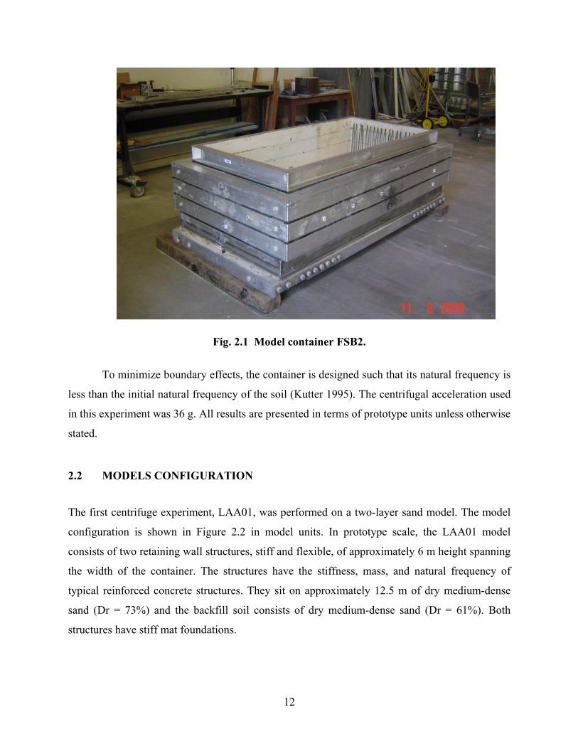
Fig. 2.1 Model container FSB2.
To minimize boundary effects, the container is designed such that its natural frequency is
less than the initial natural frequency of the soil (Kutter 1995). The centrifugal acceleration used
in this experiment was 36 g. All results are presented in terms of prototype units unless otherwise
stated.
2.2 MODELS CONFIGURATION
The first centrifuge experiment, LAA01, was performed on a two-layer sand model. The model
configuration is shown in Figure 2.2 in model units. In prototype scale, the LAA01 model
consists of two retaining wall structures, stiff and flexible, of approximately 6 m height spanning
the width of the container. The structures have the stiffness, mass, and natural frequency of
typical reinforced concrete structures. They sit on approximately 12.5 m of dry medium-dense
sand (Dr = 73%) and the backfill soil consists of dry medium-dense sand (Dr = 61%). Both
structures have stiff mat foundations.

13
Fig. 2.2 LAA01 model configuration, profile view.
The second centrifuge experiment, LAA02, was performed on a uniform density sand
model. The model configuration is shown in Figure 2.3 in model units. The LAA02 model
consists of the same stiff and flexible retaining wall structures that were used in LAA01. The
structures sit on approximately 12.5 m of dry medium-dense sand (Dr = 72%) and support a dry
medium-dense sand backfill (Dr = 72%).
Fig. 2.3 LAA02 model configuration, profile view.

14
2.3 SOIL PROPERTIES
The sand used in the two experiments was fine, uniform, angular Nevada sand. It has a mean
grain size of 0.14–0.17 mm, a uniformity coefficient of 1.67, and a specific gravity of 2.67
(Kammerer et al. 2000). The minimum and maximum dry densities determined at the University
of California, Davis, using the Japanese standard methods, yielded 14.50 and 17.49 kN/m3
respectively. The initial friction angle value for the backfill Nevada sand is estimated to be 33°
for LAA01 and 35° for LAA02 (Arulmoli et al. 1992).
2.4 STRUCTURES PROPERTIES
The model stiff and flexible structures were constructed of T6061 aluminum plate. The Young’s
modulus and Poisson’s ratio for this grade of aluminum are 10,000 ksi and 0.32, respectively.
Each structure was constructed of three plates in a tunnel-like configuration, a base plate and two
wall plates. The walls were bolted to the plates.
Both stiff and flexible aluminum structures were designed to represent typical reinforced
concrete retaining structures. Thickness of the model walls was determined by matching the
stiffness of the reinforced concrete prototypes. The stiffness of the reinforced concrete
prototypes was calculated using the effective moment of inertia of the concrete sections rather
than the gross moment of inertia (Ig = b*h3/12). The effective moment of inertia takes into
account the cracking of the concrete sections. The mass of the reinforced concrete prototypes
was also matched by adding small lead pieces to the model structures, without significantly
impacting their stiffness. Drawings of the stiff and flexible model structures are shown in Figure
2.4. The dimension of the prototype aluminum structures and their properties are presented in
Table 2.1.

15
Fig. 2.4 Stiff and flexible model structures configuration (dimensions: in.).
Table 2.1 Prototype aluminum structures dimensions and properties.
Stiff Flexible Stem Height (ft) 18.6 18.6 Stem Thickness (ft) 1.5 0.84 Stem Stiffness (lb-in.2 per ft width) 5.83E+10 1.02E+10 Base Width (ft) 35.64 36.96 Base Thickness (ft) 2.7 2.7 Base Stiffness (lb-in.2 per ft width) 3.40E+11 3.40E+11 Estimated Natural Period (sec) 0.23 0.49
2.5 MODEL PREPARATION
The sand was placed using dry pluviation in different layers underneath and behind the
structures. The height of each layer corresponds to a horizontal array of instruments, as shown in
Figures 2.2 and 2.3. The soil density was produced by calibrating the drop height, mesh opening,
and speed of drop for the pluviator. After placement of each layer, the sand surface was
smoothed with a vacuum and instruments were placed at their specific positions. Industrial
grease was placed between the structures’ walls and the container to provide a frictionless
boundary and prevent sand from passing through. Lead was added to the structures in small
pieces of 1 in.2 each in order to match the masses of the reinforced concrete structures.
Photographs of the model under construction and on the centrifuge arm are shown in Figures
2.5–2.8.

16
Fig. 2.5 Pluviation of sand inside model container.
Fig. 2.6 Leveling sand surface with a vacuum.

17
Fig. 2.7 Model under construction.
Fig. 2.8 Model on centrifuge arm.

18
2.6 INSTRUMENTATION
LAA01 and LAA02 models were densely instrumented in order to collect accurate and reliable
measurements of accelerations, displacements, shear wave velocities, strains, bending moments
and earth pressures. Horizontal and vertical accelerations in the soil and on the structures were
measured using miniature ICP and MEMs (wireless) accelerometers. Soil settlement and
structures’ deflection and settlement were measured at different locations using a combination of
LVDTs and linear potentiometers. Shear wave velocities in the soil underneath and behind the
structures were measured using bender elements and air hammers. The locations of
accelerometers, bender elements, air hammers, and displacement transducers are shown in
Figures 2.2 and 2.3. All wired instruments were sampled at a model scale sampling frequency of
4096 Hz. MEMs accelerometers were sampled at a model scale sampling frequency of 2048 Hz.
Accurate measurement of lateral earth pressure distribution was the major goal of this
study. In the past, lateral stress measurements in laboratory experiments were usually made using
pressure cells. Unfortunately, such measurements are not considered reliable due to the fact that
cell/soil reaction is a function of the relative stiffness of the cell with respect to the soil and
arching effects caused by the disturbance of the stress field by the presence of the cell
(Dewoolkar et al. 2001). Therefore, in order to avoid these problems in the experiments
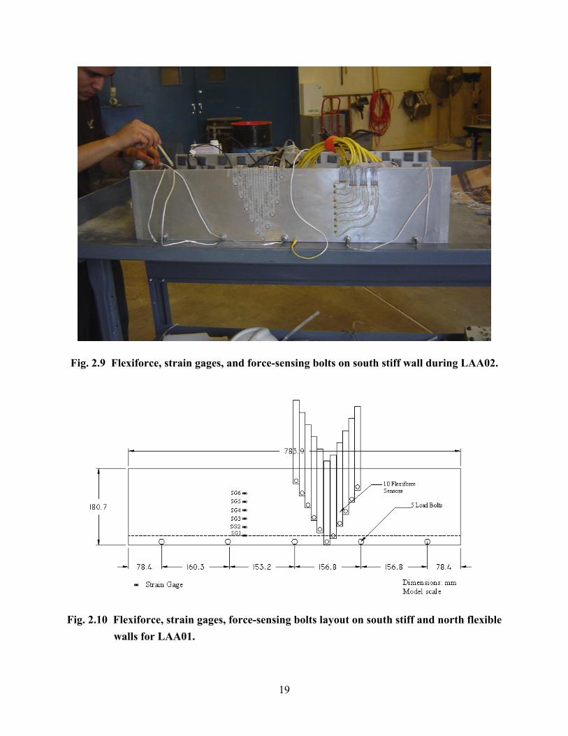
performed in this study, three different sets of instruments were used. The lateral earth pressures
were directly measured using flexible tactile pressure Flexiforce sensors. The Flexiforce sensors,
manufactured by Tekscan, are approximately 0.2 mm thick. The active sensing area is a 0.375 in.
diameter circle at the end of the sensor. The sensing area consists of conductive material
separated by semi-conductive ink, whereby the resistance is inversely proportional to the applied
force. Lateral earth pressures were also calculated by differentiating the bending moments
measured by the strain gages mounted on the model walls. Finally, direct measurements of the
total bending moments at the bases of the walls were made using force-sensing bolts at the wall-
foundation joints. The locations of the strain gages, Flexiforce sensors, and force-sensing bolts
on the south stiff and north flexible walls for experiments LAA01 and LAA02 are shown in
Figures 2.8–2.11.
19
Fig. 2.9 Flexiforce, strain gages, and force-sensing bolts on south stiff wall during LAA02.
Fig. 2.10 Flexiforce, strain gages, force-sensing bolts layout on south stiff and north flexible walls for LAA01.

20
Fig. 2.11 Flexiforce, strain gages, force-sensing bolts layout on south stiff and north flexible walls for LAA02.
2.7 CALIBRATION
Linear potentiometers, LVDTs, and strain gages were manually calibrated specifically for these
tests and compared to the manufacturer’s specifications. The accelerometers were rated using the
manufacturer’s provided instrument sensitivities.
Special calibration techniques had to be developed for the force-sensing bolts and
Flexiforce sensors, used for the first time at the Center for Geotechnical Modeling at UC Davis.
Figure 2.12 shows the calibration of the force-sensing bolts and strain gages. A uniform known
load was applied at the top of the wall and the response from the load sensing bolts and strain
gages was recorded.
The Flexiforce sensors, being very sensitive to testing conditions, were calibrated in
conditions similar to the ones expected during the experiment. Four sensors were mounted to the
base plate of a small container filled with Nevada sand. Pressure was applied to the container,
and the Flexiforce responses were recorded.
21
Fig. 2.12 Calibration of force-sensing bolts and strain gages.
2.8 SHAKING EVENTS
Five shaking events were applied to the LAA01 model in flight at 36 g centrifugal acceleration.
The shaking was applied parallel to the long sides of the model container and orthogonal to the
model structures. The shaking events consisted of a step wave, a ground motion recorded at the
Santa Cruz station during the Loma Prieta earthquake and applied three times to the model, and a
ground motion recorded at 83 m depth at Port Island during the 1995 Kobe earthquake. The
shaking events for LAA01 along with their prototype base peak accelerations are shown in Table
2.2.
Fifteen shaking events were applied to the LAA02 model in flight at 36 g centrifugal
acceleration. The shaking events consisted of step waves, ground motions recorded at the Santa
Cruz (SC) station and Saratoga West Valley College (WVC) stations during the Loma Prieta
1989 earthquake, ground motions recorded at 83 m depth at the Port Island (PI) and Takatori
(TAK) stations during the 1995 Kobe earthquake, and ground motions recorded at the Yarmica
(YPT) station during the Kocaeli, Turkey, 1999 earthquake.

22
Input ground motions for experiments LAA01 and LAA02 should reasonably reproduce
the range of frequencies present in the recorded earthquake motions. However, travel limitations
of the shaking table limit the low-frequency content of the input motions and, therefore, affect
the overall spectra of the motions. Comparison examples of four recorded earthquake motions
and their response spectra to the corresponding input motions applied to the models are shown in
Figures 2.13–2.16.

23
Original Source Record
Time [sec]32302826242220181614121086420
Acc
eler
atio
n [g
] 0.4
0.2
0
-0.2
Input Record
Time [sec]32302826242220181614121086420
Acc
eler
atio
n [g
] 0.40.2
0-0.2-0.4-0.6
Damp. 5.0%Original Source Record
Period [sec]43210
Res
pons
e A
ccel
erat
ion
[g]
1.61.41.2
10.80.60.40.2
0
Damp. 5.0%Input Record
Period [sec]43210
Res
pons
e A
ccel
erat
ion
[g]
1.5
1
0.5
0
Fig. 2.13 Comparison of original Loma Prieta-SC090 source record to input Loma Prieta-SC-1, LAA02 record and their response spectra.

24
Original Source Record
Time [sec]32302826242220181614121086420
Acc
eler
atio
n [g
] 0.60.40.2
0-0.2-0.4-0.6
Input Record
Time [sec]32302826242220181614121086420
Acc
eler
atio
n [g
]
0.5
0
-0.5
Damp. 5.0%Original Source Record
Period [sec]43210
Res
pons
e A
ccel
erat
ion
[g]
2
1.5
1
0.5
0
Damp. 5.0%Input Record
Period [sec]43210
Res
pons
e A
ccel
erat
ion
[g] 4
3.53
2.52
1.51
0.50
Fig. 2.14 Comparison of original Kobe-TAK090 source record to input Kobe-TAK090-2, LAA02 record and their response spectra.
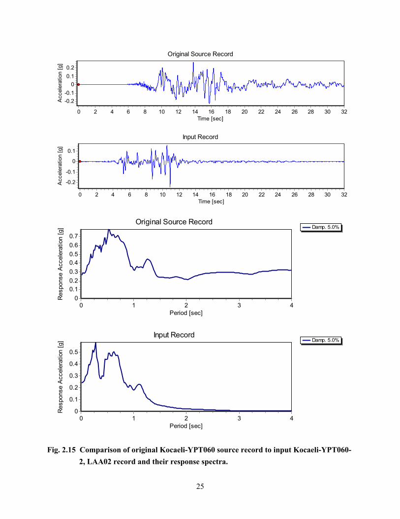
25
Original Source Record
Time [sec]32302826242220181614121086420
Acc
eler
atio
n [g
]0.20.1
0-0.1-0.2
Input Record
Time [sec]32302826242220181614121086420
Acc
eler
atio
n [g
]
0.1
0
-0.1
-0.2
Damp. 5.0%Original Source Record
Period [sec]43210
Res
pons
e A
ccel
erat
ion
[g]
0.70.60.50.40.30.20.1
0
Damp. 5.0%Input Record
Period [sec]43210
Res
pons
e A
ccel
erat
ion
[g]
0.5
0.4
0.3
0.2
0.1
0
Fig. 2.15 Comparison of original Kocaeli-YPT060 source record to input Kocaeli-YPT060-2, LAA02 record and their response spectra.

26
Original Source Record
Time [sec]32302826242220181614121086420
Acc
eler
atio
n [g
] 0.20.1
0-0.1-0.2-0.3
Input Record
Time [sec]302520151050
Acc
eler
atio
n [g
] 0.2
0.1
0
-0.1
Damp. 5.0%Original Source Record
Period [sec]43210
Res
pons
e A
ccel
erat
ion
[g]
0.70.60.50.40.30.20.1
0
Damp. 5.0%Input Record
Period [sec]43210
Res
pons
e A
ccel
erat
ion
[g] 0.6
0.5
0.4
0.3
0.2
0.1
0
Fig. 2.16 Comparison of original Loma Prieta-WVC270 source record to input Loma Prieta-WVC270-1, LAA02 record and their response spectra.

27
Since the Kobe TAK, Loma Prieta WVC, and Kocaeli YPT ground motions were used
for the first time at the centrifuge facility at UC Davis, these ground motions had to be applied
several times in order to scale the input record as close as possible to the peak accelerations and
frequency contents of the original records. The Kobe PI ground motion was applied a second
time to the model due to a power supply failure. The shaking events for LAA02 along with their
prototype base peak accelerations are shown in Table 2.3.
Table 2.2 Shaking sequence for LAA01.
Shaking Event Input Peak Acceleration (g)
Step Wave 0.06 Loma Prieta 1 - Loma Prieta 2 0.43 Kobe 0.90 Loma Prieta 3 0.43
Table 2.3 Shaking sequence for LAA02.
Shaking Event Input Peak Acceleration (g)
Step Wave-1 0.05 Loma Prieta-SC-1 0.66 Kobe-PI-1 0.79 Step Wave-2 0.05 Kobe-PI-2 0.80 Loma Prieta-SC-2 0.49 Kocaeli-YPT060-1 0.04 Kocaeli-YPT060-2 0.15 Kocaeli-YPT060-3 0.24 Kocaeli-YPT330-1 0.10 Kocaeli-YPT330-2 0.27 Kobe-TAK090-1 0.74 Kobe-TAK090-2 0.87 Loma Prieta-WVC270-1 0.23 Kocaeli-YPT330-3 0.22
2.9 LIMITATIONS
During both centrifuge experiments LAA01 and LAA02, Flexiforce sensors experienced drift,
and the original calibration factors developed for these sensors could not be applied to the
results. In order to interpret the Flexiforce voltage records, we matched the static earth pressures

28
recorded before and after each shake to the corresponding static earth pressures interpreted from
the strain gages, and new calibration factors were back-calculated to take into account the drift of
the response. These new calibration factors were applied to interpret the total dynamic earth
pressures recorded by the Flexiforce sensors. As a result of the significant drift, the results
obtained from the Flexiforce sensors were used for qualitative interpretations more than for
quantitative interpretations.
The main problems and limitations that occurred during LAA01 were that:
• During the first Loma Prieta shaking event, wired accelerometers were not set at the
appropriate gain, and accelerations were recorded only by wireless accelerometers for
this shake. As a result of this problem, the Loma Prieta shaking event was applied a
second time to the model.
• Accelerometer A12 failed during the experiment.
• SG1 on the flexible wall failed during the experiment.
• Data obtained from the bender elements located behind the retaining wall structures were
very noisy.
The main problems and limitations encountered during LAA02 were that
• A power supply failure was encountered during Kobe-PI-1 and as a result, the Kobe-PI
event preceded by a step wave was applied a second time to the model.
• Since the Kobe TAK, Loma Prieta WVC, and Kocaeli YPT ground motions were used
for the first time at the centrifuge facility at UC Davis, the original records had to be
filtered before being applied to the shaking table. Unfortunately, the filtered input
motions had different peak accelerations and frequency contents than the source motions.
• Accelerometers A28 and A31 failed during the experiment.
• SG8 on the stiff wall and SG6 and SG2 on the flexible wall failed during the experiment.
• Bender elements data were not collected after Loma Prieta-SC-1, Kobe-PI-1, and Step
Wave-2 due to technical problems.
• Air hammer data were not collected before Step Wave-1 and after Kobe-PI-1, Step
Wave-2, Loma Prieta-SC-2, and Kocaeli-YPT330-2 due to technical problems.
29
3 Experimental Results
3.1 ACCELERATION RESPONSE AND GROUND MOTION PARAMETERS
Acceleration time series were collected during both series of tests at the accelerometer locations
shown in Figure 2.2 and Figure 2.3, respectively. Acceleration time series recorded at the
northeast and northwest of the load frame were averaged to determine the input ground motion.
All horizontal acceleration recordings have been corrected so that horizontal acceleration is
positive to the south and vertical acceleration is positive downwards, regardless of the orientation
of the instruments themselves. All acceleration time series presented in this report have been
filtered and the mean was removed. Acceleration time series were filtered with a third-order
Butterworth low-pass filter with prototype scale corner frequency of 25 Hz for noise reduction,
as well as a third-order Butterworth high-pass filter with a prototype scale corner frequency of
0.3 Hz to remove the long period drift that would appear in the records after integration to
velocity and again to displacement. The disadvantage of such filtering is that any apparent
permanent offset of the instrument is also removed.
Tables 3.1 and 3.2 present the ground motion parameters for the different input shaking
events for LAA01 and LAA02, respectively. These ground motion parameters include the peak
ground acceleration (PGA), the Arias intensity (Ia), the predominant period (Tp), the mean period
(Tm) and the bracketed duration (D). D is the total time elapsed between the first and the last
excursions of a level of acceleration of 5% of the PGA. Tp is the period at which the maximum
spectral acceleration occurs in an acceleration response spectrum calculated at 5% damping. Tm
is a better frequency content characterization parameter being estimated with the following
equation, where Ci are the Fourier amplitudes, and fi represent the discrete Fourier transform
frequencies between 0.25–20 Hz.

30
Figures 3.1–3.6 present the horizontal acceleration, integrated velocity, integrated
displacement and Arias intensity time series of the input ground motions applied during LAA01.
Figures 3.7–3.17 present the horizontal acceleration, integrated velocity, integrated displacement,
and Arias intensity time series of the input ground motions applied during LAA02. The
acceleration response spectra at 5% damping are also presented for the input ground motions.
Table 3.1 Input ground motions parameters for different shaking events during LAA01.
Shaking Event PGA (g) Ia (m/sec) Tp (sec) Tm (sec) D (sec) Loma Prieta-1 - 1.19 0.34 0.53 27.06 Loma Prieta-2 0.43 1.22 0.30 0.52 23.46 Kobe 0.90 5.44 0.26 0.79 25.11 Loma Prieta-3 0.43 1.17 0.3 0.53 23.47
Table 3.2 Input ground motions parameters for different shaking events during LAA02.
Shaking Event PGA (g) Ia (m/sec) Tp (sec) Tm (sec) D (sec) Loma Prieta-SC-1 0.66 1.97 0.14 0.39 9.51 Kobe-PI-1 0.79 5.68 0.36 0.77 25.13 Kobe-PI-2 0.80 6.07 0.36 0.77 18.23 Loma Prieta-SC-2 0.49 1.33 0.3 0.52 23.45 Kocaeli-YPT060-1 0.04 0.011 0.62 0.62 23.50 Kocaeli-YPT060-2 0.15 0.12 0.28 0.54 18.60 Kocaeli-YPT060-3 0.24 0.30 0.28 0.51 15.65 Kocaeli-YPT330-1 0.10 0.054 0.20 0.57 20.41 Kocaeli-YPT330-2 0.27 0.39 0.24 0.53 15.44 Kobe-TAK090-1 0.74 4.95 0.50 0.41 8.61 Kobe-TAK090-2 0.87 6.23 0.20 0.44 16.16 Loma Prieta-WVC270 0.23 0.28 0.26 0.56 12.05 Kocaeli-YPT330-3 0.22 0.36 0.24 0.56 19.70

31
a. Horizontal Input Acceleration
Time [sec]302520151050
Acc
eler
atio
n [g
]0.2
0
-0.2
b. Horizontal Input Velocity
Time [sec]302520151050
Vel
ocity
[cm
/sec
]
20
10
0
-10
-20
c. Horizontal Input Displacement
Time [sec]302520151050D
ispl
acem
ent [
cm]
2
0
-2
-4
d. Arias Intensity
Time [sec]302520151050
Aria
s In
tens
ity (%
)
100806040200
Damp. 5.0%e. Acceleration Response Spectrum
Period [sec]43210R
espo
nse
Acc
eler
atio
n [g
]
10.80.6
0.40.2
0
Fig. 3.1 Horizontal acceleration, velocity, displacement, Arias intensity, and response spectrum of Loma Prieta-1 input motion for LAA01.

32
a. Horizontal Input Acceleration
Time [sec]302520151050
Acc
eler
atio
n [g
]0.4
0.2
0
-0.2
b. Horizontal Input Velocity
Time [sec]302520151050
Vel
ocity
[cm
/sec
]
20
100
-10-20
c. Horizontal Input Displacement
Time [sec]302520151050D
ispl
acem
ent [
cm]
2
0
-2
-4
d. Arias Intensity
Time [sec]302520151050
Aria
s In
tens
ity (%
)
100806040200
Damp. 5.0%e. Acceleration Response Spectrum
Period [sec]43210R
espo
nse
Acc
eler
atio
n [g
]
1.21
0.80.60.40.2
0
Fig. 3.2 Horizontal acceleration, velocity, displacement, Arias intensity, and response spectrum of Loma Prieta-2 input motion for LAA01.

33
a. Horizontal Input Acceleration
Time [sec]35302520151050
Acc
eler
atio
n [g
]0.5
0
-0.5
b. Horizontal Input Velocity
Time [sec]35302520151050
Vel
ocity
[cm
/sec
]
50
0
-50
c. Horizontal Input Displacement
Time [sec]35302520151050D
ispl
acem
ent [
cm]
20
10
0
-10
d. Arias Intensity
Time [sec]35302520151050
Aria
s In
tens
ity (%
)
100806040200
Damp. 5.0%e. Acceleration Response Spectrum
Period [sec]43210R
espo
nse
Acc
eler
atio
n [g
]
1.5
1
0.5
0
Fig. 3.3 Horizontal acceleration, velocity, displacement, Arias intensity, and response spectrum of Kobe input motion for LAA01.

34
a. Horizontal Input Acceleration
Time [sec]302520151050
Acc
eler
atio
n [g
]0.4
0.2
0
-0.2
b. Horizontal Input Velocity
Time [sec]302520151050
Vel
ocity
[cm
/sec
]
20
10
0
-10
-20
c. Horizontal Input Displacement
Time [sec]302520151050D
ispl
acem
ent [
cm]
2
0
-2
d. Arias Intensity
Time [sec]302520151050
Aria
s In
tens
ity (%
)
100806040200
Damp. 5.0%e. Acceleration Response Spectrum
Period [sec]43210R
espo
nse
Acc
eler
atio
n [g
]
10.80.60.40.2
0
Fig. 3.4 Horizontal acceleration, velocity, displacement, Arias intensity, and response spectrum of Loma Prieta-3 input motion for LAA01.

35
a. Horizontal Input Acceleration
Time [sec]302520151050
Acc
eler
atio
n [g
]
0.5
0
-0.5
b. Horizontal Input Velocity
Time [sec]302520151050
Vel
ocity
[cm
/sec
]
20
0
-20
c. Horizontal Input Displacement
Time [sec]302520151050D
ispl
acem
ent [
cm]
2
0
-2
d. Arias Intensity
Time [sec]302520151050
Aria
s In
tens
ity (%
)
100806040200
Damp. 5.0%e. Acceleration Response Spectrum
Period [sec]987654321R
espo
nse
Acc
eler
atio
n [g
]
1.5
1
0.5
0
Fig. 3.5 Horizontal acceleration, velocity, displacement, Arias intensity, and response spectrum of Loma Prieta-SC-1 input motion during LAA02.

36
a. Horizontal Input Acceleration
Time [sec]302520151050
Acc
eler
atio
n [g
]0.5
0
-0.5
b. Horizontal Input Velocity
Time [sec]302520151050
Vel
ocity
[cm
/sec
]
50
0
-50
c. Horizontal Input Displacement
Time [sec]302520151050D
ispl
acem
ent [
cm]
10
0
-10
d. Arias Intensity
Time [sec]302520151050
Aria
s In
tens
ity (%
)
100806040200
Damp. 5.0%e. Acceleration Response Spectrum
Period [sec]987654321R
espo
nse
Acc
eler
atio
n [g
]
1.5
1
0.5
0
Fig. 3.6 Horizontal acceleration, velocity, displacement, Arias intensity, and response spectrum of Kobe-PI-1 input motion during LAA02.
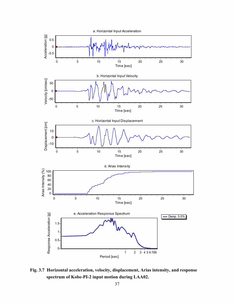
37
a. Horizontal Input Acceleration
Time [sec]302520151050
Acc
eler
atio
n [g
]0.5
0
-0.5
b. Horizontal Input Velocity
Time [sec]302520151050
Vel
ocity
[cm
/sec
]
50
0
-50
c. Horizontal Input Displacement
Time [sec]302520151050D
ispl
acem
ent [
cm]
10
0
-10
d. Arias Intensity
Time [sec]302520151050
Aria
s In
tens
ity (%
)
100806040200
Damp. 5.0%e. Acceleration Response Spectrum
Period [sec]987654321R
espo
nse
Acc
eler
atio
n [g
]
1.5
1
0.5
0
Fig. 3.7 Horizontal acceleration, velocity, displacement, Arias intensity, and response spectrum of Kobe-PI-2 input motion during LAA02.

38
a. Horizontal Input Acceleration
Time [sec]302520151050
Acc
eler
atio
n [g
]
0.40.2
0-0.2
b. Horizontal Input Velocity
Time [sec]302520151050
Vel
ocity
[cm
/sec
]
20100
-10-20
c. Horizontal Input Displacement
Time [sec]302520151050D
ispl
acem
ent [
cm]
420
-2-4
d. Arias Intensity
Time [sec]302520151050
Aria
s In
tens
ity (%
)
100806040200
Damp. 5.0%e. Acceleration Response Spectrum
Period [sec]987654321R
espo
nse
Acc
eler
atio
n [g
]
1.21
0.80.60.40.2
0
Fig. 3.8 Horizontal acceleration, velocity, displacement, Arias intensity, and response spectrum of Loma Prieta-SC-2 input motion during LAA02.

39
a. Horizontal Input Acceleration
Time [sec]302520151050
Acc
eler
atio
n [g
]
0.02
0
-0.02
-0.04
b. Horizontal Input Velocity
Time [sec]302520151050
Vel
ocity
[cm
/sec
]
2
0
-2
c. Horizontal Input Displacement
Time [sec]302520151050D
ispl
acem
ent [
cm]
0.4
0.2
0
-0.2
d. Arias Intensity
Time [sec]302520151050
Aria
s In
tens
ity (%
)
100806040200
Damp. 5.0%e. Acceleration Response Spectrum
Period [sec]987654321R
espo
nse
Acc
eler
atio
n [g
]
0.1
0.08
0.06
0.04
0.02
0
Fig. 3.9 Horizontal acceleration, velocity, displacement, Arias intensity, and response spectrum of Kocaeli-YPT060-1 input motion during LAA02.

40
a. Horizontal Input Acceleration
Time [sec]302520151050
Acc
eler
atio
n [g
]
0.050
-0.05-0.1
-0.15
b. Horizontal Input Velocity
Time [sec]302520151050
Vel
ocity
[cm
/sec
]
5
0
-5
-10
c. Horizontal Input Displacement
Time [sec]302520151050D
ispl
acem
ent [
cm]
10.5
0-0.5
d. Arias Intensity
Time [sec]302520151050
Aria
s In
tens
ity (%
)
100806040200
Damp. 5.0%e. Acceleration Response Spectrum
Period [sec]987654321R
espo
nse
Acc
eler
atio
n [g
]
0.30.250.2
0.150.1
0.050
Fig. 3.10 Horizontal acceleration, velocity, displacement, Arias intensity, and response spectrum of Kocaeli-YPT060-2 input motion during LAA02.
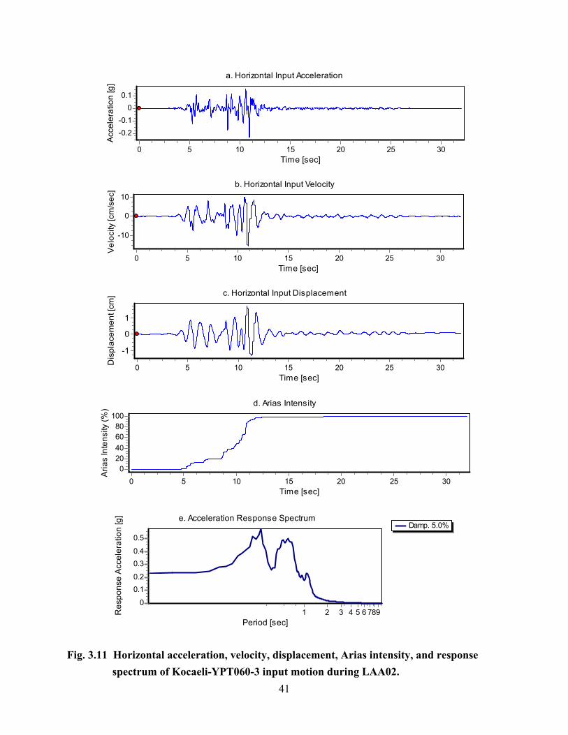
41
a. Horizontal Input Acceleration
Time [sec]302520151050
Acc
eler
atio
n [g
]
0.10
-0.1-0.2
b. Horizontal Input Velocity
Time [sec]302520151050
Vel
ocity
[cm
/sec
]
10
0
-10
c. Horizontal Input Displacement
Time [sec]302520151050D
ispl
acem
ent [
cm]
1
0
-1
d. Arias Intensity
Time [sec]302520151050
Aria
s In
tens
ity (%
)
100806040200
Damp. 5.0%e. Acceleration Response Spectrum
Period [sec]987654321R
espo
nse
Acc
eler
atio
n [g
]
0.5
0.40.3
0.20.1
0
Fig. 3.11 Horizontal acceleration, velocity, displacement, Arias intensity, and response spectrum of Kocaeli-YPT060-3 input motion during LAA02.

42
a. Horizontal Input Acceleration
Time [sec]302520151050
Acc
eler
atio
n [g
]
0.05
0
-0.05
b. Horizontal Input Velocity
Time [sec]302520151050
Vel
ocity
[cm
/sec
]
0
-5
c. Horizontal Input Displacement
Time [sec]302520151050D
ispl
acem
ent [
cm]
0.5
0
-0.5
d. Arias Intensity
Time [sec]302520151050
Aria
s In
tens
ity (%
)
100806040200
Damp. 5.0%e. Acceleration Response Spectrum
Period [sec]987654321R
espo
nse
Acc
eler
atio
n [g
]
0.2
0.15
0.1
0.05
0
Fig. 3.12 Horizontal acceleration, velocity, displacement, Arias intensity, and response spectrum of Kocaeli-YPT330-1 input motion during LAA02.

43
a. Horizontal Input Acceleration
Time [sec]302520151050
Acc
eler
atio
n [g
]
0.20.1
0-0.1-0.2
b. Horizontal Input Velocity
Time [sec]302520151050
Vel
ocity
[cm
/sec
]
10
0
-10
-20
c. Horizontal Input Displacement
Time [sec]302520151050D
ispl
acem
ent [
cm]
1
0
-1
d. Arias Intensity
Time [sec]302520151050
Aria
s In
tens
ity (%
)
100806040200
Damp. 5.0%e. Acceleration Response Spectrum
Period [sec]987654321R
espo
nse
Acc
eler
atio
n [g
]
0.5
0.40.3
0.20.1
0
Fig. 3.13 Horizontal acceleration, velocity, displacement, Arias intensity, and response spectrum of Kocaeli-YPT330-2 input motion during LAA02.

44
a. Horizontal Input Acceleration
Time [sec]302520151050
Acc
eler
atio
n [g
]
0.5
0
-0.5
b. Horizontal Input Velocity
Time [sec]302520151050
Vel
ocity
[cm
/sec
]
40200
-20-40
c. Horizontal Input Displacement
Time [sec]302520151050D
ispl
acem
ent [
cm]
2
0
-2
-4
d. Arias Intensity
Time [sec]302520151050
Aria
s In
tens
ity (%
)
100806040200
Damp. 5.0%e. Acceleration Response Spectrum
Period [sec]987654321R
espo
nse
Acc
eler
atio
n [g
]
32.5
21.5
10.5
0
Fig. 3.14 Horizontal acceleration, velocity, displacement, Arias intensity, and response spectrum of Kobe-TAK090-1 input motion during LAA02.

45
a. Horizontal Input Acceleration
Time [sec]302520151050
Acc
eler
atio
n [g
]0.5
0
-0.5
b. Horizontal Input Velocity
Time [sec]302520151050
Vel
ocity
[cm
/sec
] 40
20
0
-20
-40
c. Horizontal Input Displacement
Time [sec]302520151050D
ispl
acem
ent [
cm]
5
0
-5
d. Arias Intensity
Time [sec]302520151050
Aria
s In
tens
ity (%
)
100806040200
Damp. 5.0%e. Acceleration Response Spectrum
Period [sec]987654321R
espo
nse
Acc
eler
atio
n [g
]
3
2
1
0
Fig. 3.15 Horizontal acceleration, velocity, displacement, Arias intensity, and response spectrum of Kobe-TAK090-2 input motion during LAA02.

46
a. Horizontal Input Acceleration
Time [sec]302520151050
Acc
eler
atio
n [g
]
0.2
0.1
0
-0.1
b. Horizontal Input Velocity
Time [sec]302520151050
Vel
ocity
[cm
/sec
]
10
0
-10
c. Horizontal Input Displacement
Time [sec]302520151050D
ispl
acem
ent [
cm]
10
-1-2
d. Arias Intensity
Time [sec]302520151050
Aria
s In
tens
ity (%
)
100806040200
Damp. 5.0%e. Acceleration Response Spectrum
Period [sec]987654321R
espo
nse
Acc
eler
atio
n [g
]
0.60.50.40.30.20.1
0
Fig. 3.16 Horizontal acceleration, velocity, displacement, Arias intensity, and response spectrum of Loma Prieta-WVC270 input motion during LAA02.

47
a. Horizontal Input Acceleration
Time [sec]302520151050
Acc
eler
atio
n [g
]0.1
0
-0.1
-0.2
b. Horizontal Input Velocity
Time [sec]302520151050
Vel
ocity
[cm
/sec
]
10
0
-10
-20
c. Horizontal Input Displacement
Time [sec]302520151050D
ispl
acem
ent [
cm]
2
1
0-1
d. Arias Intensity
Time [sec]302520151050
Aria
s In
tens
ity (%
)
100806040200
Damp. 5.0%e. Acceleration Response Spectrum
Period [sec]987654321R
espo
nse
Acc
eler
atio
n [g
]
0.5
0.4
0.3
0.2
0.1
0
Fig. 3.17 Horizontal acceleration, velocity, displacement, Arias intensity, and response spectrum of Kocaeli-YPT330-3 input motion during LAA02.
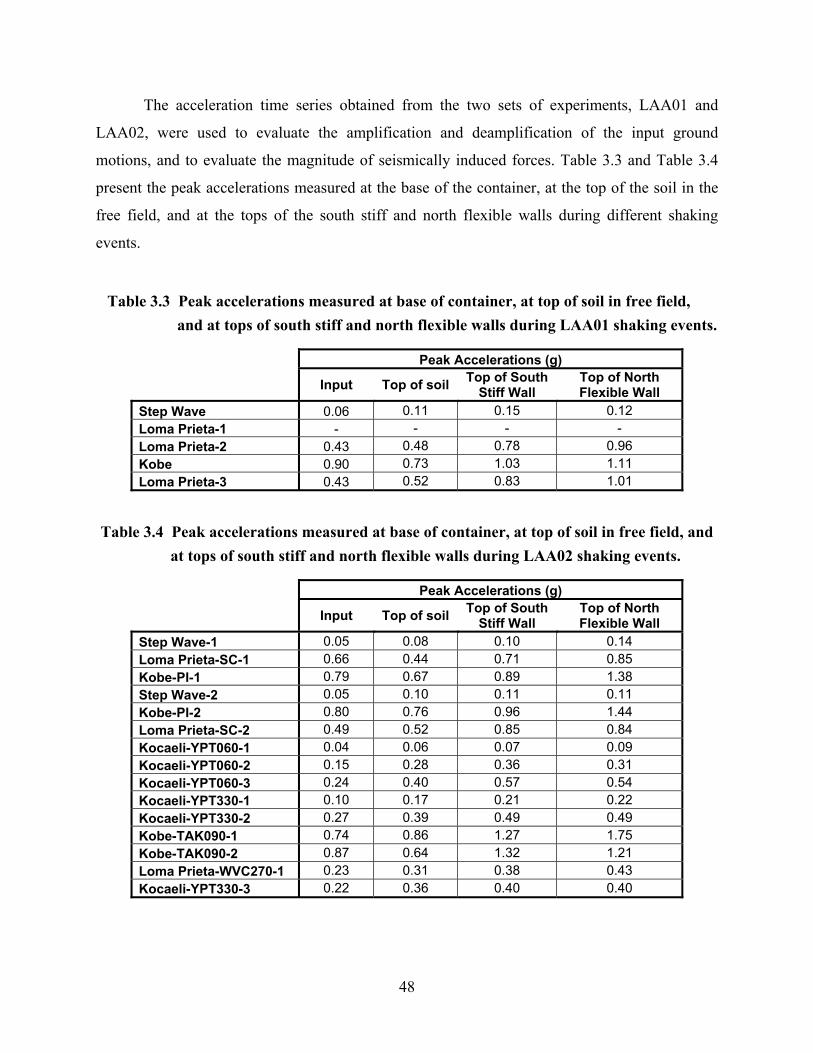
48
The acceleration time series obtained from the two sets of experiments, LAA01 and
LAA02, were used to evaluate the amplification and deamplification of the input ground
motions, and to evaluate the magnitude of seismically induced forces. Table 3.3 and Table 3.4
present the peak accelerations measured at the base of the container, at the top of the soil in the
free field, and at the tops of the south stiff and north flexible walls during different shaking
events.
Table 3.3 Peak accelerations measured at base of container, at top of soil in free field, and at tops of south stiff and north flexible walls during LAA01 shaking events.
Peak Accelerations (g)
Input Top of soil Top of South Stiff Wall
Top of North Flexible Wall
Step Wave 0.06 0.11 0.15 0.12 Loma Prieta-1 - - - - Loma Prieta-2 0.43 0.48 0.78 0.96 Kobe 0.90 0.73 1.03 1.11 Loma Prieta-3 0.43 0.52 0.83 1.01
Table 3.4 Peak accelerations measured at base of container, at top of soil in free field, and at tops of south stiff and north flexible walls during LAA02 shaking events.
Peak Accelerations (g)
Input Top of soil Top of South Stiff Wall
Top of North Flexible Wall
Step Wave-1 0.05 0.08 0.10 0.14 Loma Prieta-SC-1 0.66 0.44 0.71 0.85 Kobe-PI-1 0.79 0.67 0.89 1.38 Step Wave-2 0.05 0.10 0.11 0.11 Kobe-PI-2 0.80 0.76 0.96 1.44 Loma Prieta-SC-2 0.49 0.52 0.85 0.84 Kocaeli-YPT060-1 0.04 0.06 0.07 0.09 Kocaeli-YPT060-2 0.15 0.28 0.36 0.31 Kocaeli-YPT060-3 0.24 0.40 0.57 0.54 Kocaeli-YPT330-1 0.10 0.17 0.21 0.22 Kocaeli-YPT330-2 0.27 0.39 0.49 0.49 Kobe-TAK090-1 0.74 0.86 1.27 1.75 Kobe-TAK090-2 0.87 0.64 1.32 1.21 Loma Prieta-WVC270-1 0.23 0.31 0.38 0.43 Kocaeli-YPT330-3 0.22 0.36 0.40 0.40

49
Figure 3.18 is a plot of the peak accelerations measured at the base of the container
versus those measured at the top of the soil in the free field, at the top of the south stiff wall, and
at the top of the north flexible wall during the different shaking events. A 45° line is displayed
for reference. Based on Tables 3.3 and 3.4 and Figure 3.20, the motions are consistently
amplified at the tops of the walls, and the acceleration at the top of the soil crosses over the 45°
line, indicating attenuation of the large magnitude input shaking events.
0.05
0.25
0.45
0.65
0.85
1.05
1.25
1.45
1.65
0.05 0.25 0.45 0.65 0.85 1.05 1.25 1.45 1.65
Input Base Acc. (g)
Top
Acc
. (g)
45degree Line
South Stiff Wall
North Flexible Wall
Soil, Free Field
Fig. 3.18 Base motion amplification/deamplification for soil, stiff, and flexible structures.
3.2 SOIL SETTLEMENT AND DENSIFICATION
Vertical soil deformation measurements were recorded at the soil surface and at the foundation
level of each structure, as shown in Figure 2.2 and Figure 2.3 for LAA01 and LAA02,
respectively. The static offsets measured by the displacement transducers were used to determine
the settlement increment of the uniform density soil model after the different shaking events in
experiment LAA02. In experiment LAA01, the settlement increment of the backfill soil as well
as the soil underneath the structures (base soil) was determined for the two-layer model. Table

50
3.5 and Table 3.6 show these settlement values along with the relative density (Dr) of the soil
after each shaking event for LAA01 and LAA02, respectively. It is apparent that the maximum
settlement occurred during the first Kobe event in both sets of experiments, LAA01 and LAA02,
due to the large magnitude of shaking the relatively low initial density of the sand.
Table 3.5 Soil settlement and relative density after different shaking events for LAA01.
Base Soil Backfill
Shaking Event Settlement Increment (mm) Dr (%) Settlement
Increment (mm) Dr (%)
Step Wave 0.36 74.4 0.50 61.7 Loma Prieta-1 31.64 75.6 22.75 63.5 Loma Prieta-2 17.85 76.4 2.37 63.7 Kobe 37.62 77.9 37.34 66.7 Loma Prieta-3 4.17 78.1 5.16 67.1
Table 3.6 Soil settlement and relative density after different shaking events for LAA02.
Shaking Event Settlement Increment (mm) Dr (%)
Step Wave-1 0.36 72.1 Loma Prieta-SC-1 52.62 73.9 Kobe-PI-1 98.51 77.0 Step Wave 2 0 77.0 Kobe-PI-2 56.07 78.8 Loma Prieta-SC-2 7.00 79.05 Kocaeli-YPT060-1 0 79.05 Kocaeli-YPT060-2 1.39 79.1 Kocaeli-YPT060-3 1.82 79.1 Kocaeli-YPT330-1 0 79.1 Kocaeli-YPT330-2 0.93 79.2 Kobe-TAK090-1 29.03 80.3 Kobe-TAK090-2 16.40 81.0 Loma Prieta-WVC270 0.31 81.0 Kocaeli-YPT330-3 0.07 81.0
3.3 SHEAR WAVE VELOCITY
Bender element arrays were used to measure shear wave velocities in experiment LAA01 after
each shaking event in the soil behind and underneath the retaining wall structures as shown in
Figure 2.2. The shear wave velocities measured between the different shaking events in the base
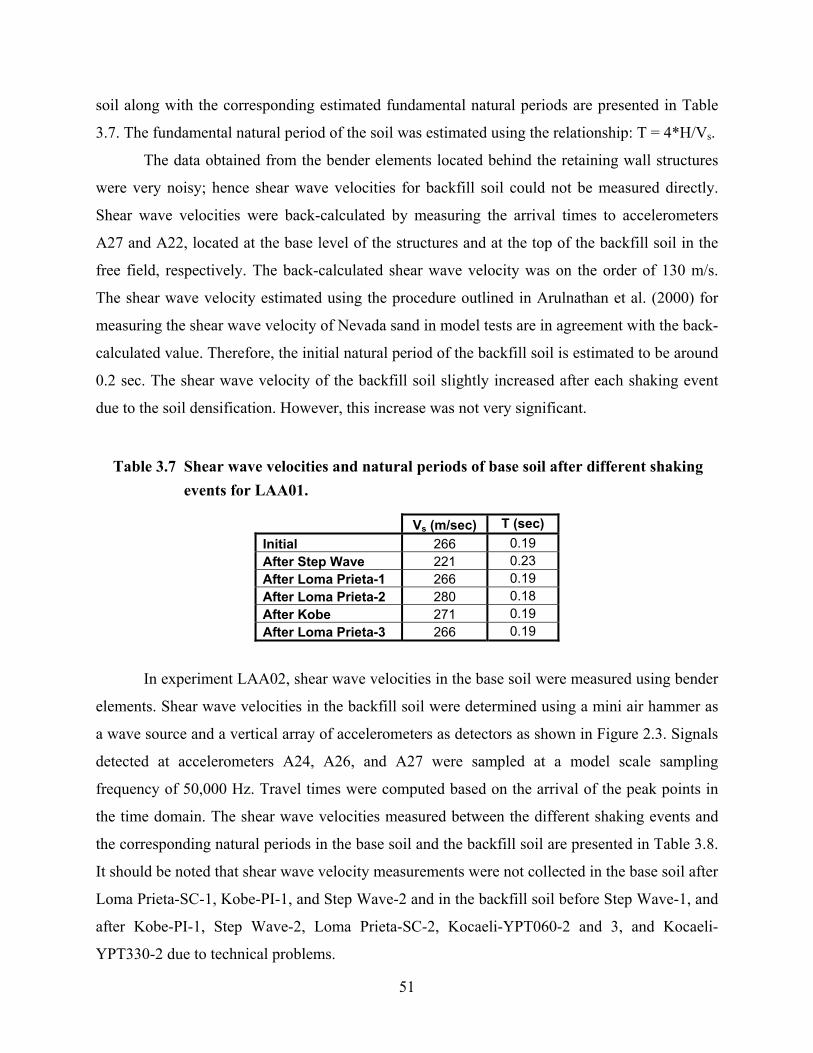
51
soil along with the corresponding estimated fundamental natural periods are presented in Table
3.7. The fundamental natural period of the soil was estimated using the relationship: T = 4*H/Vs.
The data obtained from the bender elements located behind the retaining wall structures
were very noisy; hence shear wave velocities for backfill soil could not be measured directly.
Shear wave velocities were back-calculated by measuring the arrival times to accelerometers
A27 and A22, located at the base level of the structures and at the top of the backfill soil in the
free field, respectively. The back-calculated shear wave velocity was on the order of 130 m/s.
The shear wave velocity estimated using the procedure outlined in Arulnathan et al. (2000) for
measuring the shear wave velocity of Nevada sand in model tests are in agreement with the back-
calculated value. Therefore, the initial natural period of the backfill soil is estimated to be around
0.2 sec. The shear wave velocity of the backfill soil slightly increased after each shaking event
due to the soil densification. However, this increase was not very significant.
Table 3.7 Shear wave velocities and natural periods of base soil after different shaking events for LAA01.
Vs (m/sec) T (sec) Initial 266 0.19 After Step Wave 221 0.23 After Loma Prieta-1 266 0.19 After Loma Prieta-2 280 0.18 After Kobe 271 0.19 After Loma Prieta-3 266 0.19
In experiment LAA02, shear wave velocities in the base soil were measured using bender
elements. Shear wave velocities in the backfill soil were determined using a mini air hammer as
a wave source and a vertical array of accelerometers as detectors as shown in Figure 2.3. Signals
detected at accelerometers A24, A26, and A27 were sampled at a model scale sampling
frequency of 50,000 Hz. Travel times were computed based on the arrival of the peak points in
the time domain. The shear wave velocities measured between the different shaking events and
the corresponding natural periods in the base soil and the backfill soil are presented in Table 3.8.
It should be noted that shear wave velocity measurements were not collected in the base soil after
Loma Prieta-SC-1, Kobe-PI-1, and Step Wave-2 and in the backfill soil before Step Wave-1, and
after Kobe-PI-1, Step Wave-2, Loma Prieta-SC-2, Kocaeli-YPT060-2 and 3, and Kocaeli-
YPT330-2 due to technical problems.

52
Table 3.8 Shear wave velocities and natural periods of base soil and backfill soil after different shaking events for LAA02.
Base Soil Backfill Soil Vs (m/sec) T (sec) Vs (m/sec) T (sec) Before Step Wave-1 260.74 0.19 - - After Step Wave-1 261.29 0.19 180.45 0.14 After Loma Prieta-SC-1 - - 172.55 0.15 After Kobe-PI-1 - - - - After Step Wave-2 - - - - After Kobe-PI-2 261.68 0.19 165.2 0.16 After Loma Prieta-SC-2 264.03 0.19 - After Kocaeli-YPT060-1 261.45 0.19 127.85 0.20 After Kocaeli-YPT060-2 265.55 0.19 - - After Kocaeli-YPT060-3 255.41 0.20 - - After Kocaeli-YPT330-1 256.75 0.19 127.85 0.20 After Kocaeli-YPT330-2 256.21 0.20 - - After Kobe-TAK090-1 267.12 0.19 127.85 0.20 After Kobe-TAK090-2 266.67 0.19 137.69 0.19 After Loma Prieta-WVC270-1 266.91 0.19 137.69 0.19 After Kocaeli-YPT330-3 267.12 0.19 137.69 0.19
Recall that the estimated natural period of the stiff and flexible structures was 0.23 and 0.49 sec,
respectively (Table 2.1). Thus the measured site periods were close to the natural period of the
stiff structure in both sets of experiments. Similarly the input motions had dominant periods
ranging from 0.14 to 0.62 sec and mean periods ranging from 0.39 to 0.79 sec (Tables 3.1 and
3.2), which effectively spanned the range of periods expected to produce maximum response in
the soil deposit and structures.
3.4 MOMENT DISTRIBUTIONS
3.4.1 Analysis Procedure and Assumptions
Five force-sensing bolts and six strain gages were used to instrument the south stiff and north
flexible walls in experiment LAA01, as shown in Figure 2.9. The total dynamic moment
distributions along the heights of the walls were calculated from the strain values measured by
the strain gages. For the stiff wall, six dynamic moment profiles were computed for each shaking
event; each moment profile corresponding to the time at which the maximum moment occurred
at one strain gage location and plotting the moments recorded at the other strain gages at the

53
same time. For the flexible wall, applying the same procedure, five moment profiles were plotted
for each shaking event instead of six, since the strain gage SG1 was damaged. The dynamic
moment profiles for the same shaking event were very similar for both the stiff and the flexible
walls, with the envelope consistently occurring at the time the maximum moment was recorded
at SG1 for the stiff wall and SG2 for the flexible walls. Therefore, all maximum total dynamic
moment profiles and all maximum dynamic moment increment profiles observed in experiment
LAA01 which are presented in this section correspond to the times at which the maximum
moments occurred at SG1 and SG2 for the stiff and the flexible walls, respectively. The dynamic
moments at the bases of the walls were directly measured by the force-sensing bolts, applying
the appropriate moment calibration factors.
In experiment LAA02 the south stiff and north flexible walls were instrumented with five
force-sensing bolts and eight strain gages each, as shown in Figure 2.11. SG8 on the stiff wall
and SG6 on the flexible wall did not usually give good records. The same procedure outlined
above for experiment LAA01 was used to obtain the maximum total dynamic moment and
dynamic moment increment profiles. Therefore, all maximum total dynamic moment profiles
and all maximum dynamic moment increment profiles for LAA02 presented in this section
correspond to the times at which the maximum moments occurred at SG1 for the stiff and
flexible walls, respectively. The dynamic moments at the bases of the walls were directly
measured by the force-sensing bolts, applying the appropriate moment calibration factors.
For comparison, we estimated the total dynamic moments as well as the dynamic moment
increments acting at the bases of the walls applying the M-O method, the Seed and Whitman
(1970) method, and the BART design criteria. For the M-O method, the resultant force of the
total dynamic pressure distribution was applied at one third the height of the wall from its base.
For the Seed and Whitman (1970) method, we used the M-O pressure distribution with the
resultant force of the dynamic increment applied at two thirds the height of the wall from the
base. The peak ground acceleration values recorded at the accelerometers located at the top of
the soil in the free field as well as 65% the peak ground accelerations were used in the M-O and
Seed and Whitman (1970) estimates.
The BART design criteria for stiff walls assume at-rest (Ko) earth pressures for static
loads and 1.5 times the M-O inverted triangular pressure increment for seismic loads. For
flexible walls, BART design criteria assume active earth pressures for static loads and the M-O
inverted triangular pressure increment for seismic loads. For both stiff and flexible walls, half the
54
peak ground accelerations measured at the top of the soil in the free field were used for moment
estimations using the BART design criteria.
3.4.2 Results: Time Series
Strain time series recorded during experiments LAA01 and LAA02 were filtered using a first-
order low-pass Butterworth filter with a prototype scale corner frequency of 25 Hz for noise
reduction. Moment time series recorded by the force-sensing bolts were filtered using a third-
order low-pass Butterworth filter with a prototype scale corner frequency of 25 Hz for noise
reduction.
In experiment LAA01, strain gage SG1 on the flexible wall was damaged, thus moment
time series at this location were not presented for the flexible wall. Moreover, one force-sensing
bolt on the flexible wall failed at the beginning of the experiment. The moment carried by this
bolt was estimated based on the calibration data.
In experiment LAA02, SG7, and SG8 on the stiff and flexible walls did not generally
give good results during some of the shakes. Moreover, a power supply problem was
encountered during the Kobe-PI-1 shake and the strain gage and force-sensing bolts time series
from this shake were very noisy. The moment time series obtained during the Kocaeli-YPT060-1
and Kocaeli-YPT330-1 are not presented in this report due to the insignificant magnitude of
shaking. We also note that the moment time series obtained from SG1 on the stiff wall were
consistently less than the moment time series obtained from other strain gages on the same wall
which suggests that SG1 results might not be accurate. A data-acquisition problem was
encountered on one force-sensing bolt channel on the north flexible wall during the Step Wave-
1, Loma Prieta-SC-1, and Kobe-PI-1 shaking events. The moment carried by this bolt during
these shakes was estimated based on the calibration data. The problem was resolved before the
Step Wave-2 shake. Moreover, one force-sensing bolt on the stiff wall gave bad moment time
series during all events. The moment carried by this bolt was estimated based on the calibration
data.

55
3.4.3 Static Moments
Figures 3.19–3.24 present the static moment profiles measured by the strain gages on the south
stiff and north flexible walls before the initial shake in both experiments and between the
successive shaking events. The static moments measured at the bases of the walls as well as the
static at-rest and static active moment estimates are included in Figures 3.19–3.24 for
comparison. The static at-rest and static active moments were estimated using an initial friction
angle of 33° in experiment LAA01 and 35° in experiment LAA02. In experiment LAA02 the
initial friction angle was assumed to increase gradually toward a final value of 36 to reflect the
densification of the soil during each successive shaking event.
Initial - Before ShakingLAA01
0
50
100
150
200
0 20 40 60x106
Static Moment (lb-in)
Z (in
)
Meas. SG-Stiff
Meas. SG-Flexible
Meas. LB-Stiff
Meas. LB-Flexible
Static At Rest
Static Active
Initial - Before ShakingLAA02
0
50
100
150
200
0 20 40 60x106
Static Moment (lb-in)
Z (in
)
Meas. SG-Stiff
Meas. SG-Flexible
Meas. LB-Stiff
Meas. LB-Flexible
Static At Rest
Static Active
Fig. 3.19 Static moment profiles measured by strain gages and force-sensing bolts and estimated using static at-rest and static active pressure distributions before shaking LAA01 and LAA02 models.

56
After Loma Prieta-1LAA01
0
50
100
150
200
0 20 40 60x106
Static Moment (lb-in)Z
(in)
Meas. SG-Stiff
Meas. SG-Flexible
Meas. LB-Stiff
Meas. LB-Flexible
Static At Rest
Static Active
After Loma Prieta-SC-1LAA02
0
50
100
150
200
0 20 40 60x106
Static Moment (lb-in)
Z (in
)
Meas. SG-Stiff
Meas. SG-Flexible
Meas. LB-Stiff
Meas. LB-Flexible
Static At Rest
Static Active
After Loma Prieta-2LAA01
0
50
100
150
200
0 20 40 60x106
Static Moment (lb-in)
Z (in
)
Meas. SG-Stiff
Meas. SG-Flexible
Meas. LB-Stiff
Meas. LB-Flexible
Static At Rest
Static Active
Fig. 3.20 Static moment profiles measured by strain gages and force-sensing bolts and estimated using static at-rest and static active pressure distributions after Loma Prieta-1 and 2 for LAA01 and after Loma Prieta-SC-1 for LAA02.

57
After KobeLAA01
0
50
100
150
200
0 20 40 60x106
Static Moment (lb-in)
Z (in
)
Meas. SG-Stiff
Meas. SG-Flexible
Meas. LB-Stiff
Meas. LB-Flexible
Static At Rest
Static Active
After Kobe-PI-1LAA02
0
50
100
150
200
0 20 40 60x106
Static Moment (lb-in)
Z (in
)
Meas. SG-Stiff
Meas. SG-Flexible
Meas. LB-Stiff
Meas. LB-Flexible
Static At Rest
Static Active
After Kobe-PI-2LAA02
0
50
100
150
200
0 20 40 60x106
Static Moment (lb-in)
Z (in
)
Meas. SG-Stiff
Meas. SG-Flexible
Meas. LB-Stiff
Meas. LB-Flexible
Static At Rest
Static Active
Fig. 3.21 Static moment profiles measured by strain gages and force-sensing bolts and estimated using static at-rest and static active pressure distributions after Kobe for LAA01 and after Kobe-PI-1 and -2 for LAA02.

58
After Loma Prieta-3LAA01
0
50
100
150
200
0 20 40 60x106
Static Moment (lb-in)Z
(in)
Meas. SG-Stiff
Meas. SG-Flexible
Meas. LB-Stiff
Meas. LB-Flexible
Static At Rest
Static Active
After Loma Prieta-SC-2LAA02
0
50
100
150
200
0 20 40 60x106
Static Moment (lb-in)
Z (in
)
Meas. SG-Stiff
Meas. SG-Flexible
Meas. LB-Stiff
Meas. LB-Flexible
Static At Rest
Static Active
After Kocaeli-YPT060-2LAA02
0
50
100
150
200
0 20 40 60x106
Static Moment (lb-in)
Z (in
)
Meas. SG-Stiff
Meas. SG-Flexible
Meas. LB-Stiff
Meas. LB-Flexible
Static At Rest
Static Active
After Kocaeli-YPT060-3LAA02
0
50
100
150
200
0 20 40 60x106
Static Moment (lb-in)
Z (in
)
Meas. SG-Stiff
Meas. SG-Flexible
Meas. LB-Stiff
Meas. LB-Flexible
Static At Rest
Static Active
Fig. 3.22 Static moment profiles measured by strain gages and force-sensing bolts and estimated using static at-rest and static active pressure distributions after Loma Prieta-3 for LAA01 and after Loma Prieta-SC-2, and Kocaeli-YPT060-2 and -3 for LAA02.

59
After Kocaeli-YPT330-2LAA02
0
50
100
150
200
0 20 40 60x106
Static Moment (lb-in)Z
(in)
Meas. SG-Stiff
Meas. SG-Flexible
Meas. LB-Stiff
Meas. LB-Flexible
Static At Rest
Static Active
Kobe-TAK090-1LAA02
0
50
100
150
200
0 20 40 60x106
Total Dynamic Moment (lb-in)
Z (in
)
Meas. SG-Stiff
Meas. SG-Flexible
Meas. LB-Stiff
Meas. LB-Flexible
Static At Rest
Static Active
After Kobe-TAK090-2LAA02
0
50
100
150
200
0 20 40 60x106
Static Moment (lb-in)
Z (in
)
Meas. SG-Stiff
Meas. SG-Flexible
Meas. LB-Stiff
Meas. LB-Flexible
Static At Rest
Static Active
After Loma Prieta-WVC270LAA02
0
50
100
150
200
0 20 40 60x106
Static Moment (lb-in)
Z (in
)
Meas. SG-Stiff
Meas. SG-Flexible
Meas. LB-Stiff
Meas. LB-Flexible
Static At Rest
Static Active
Fig. 3.23 Static moment profiles measured by strain gages and force-sensing bolts and estimated using static at-rest and static active pressure distributions after Kocaeli-YPT330-2, Kobe-TAK090-1 and -2, and Loma Prieta-WVC270 for LAA02.

60
After Kocaeli-YPT330-3LAA02
0
50
100
150
200
0 20 40 60x106
Static Moment (lb-in)
Z (in
)
Meas. SG-Stiff
Meas. SG-Flexible
Meas. LB-Stiff
Meas. LB-Flexible
Static At Rest
Static Active
Fig. 3.24 Static moment profiles measured by strain gages and force-sensing bolts and estimated using static at-rest and static active pressure distributions after Kocaeli-YPT330-3 for LAA02.
As shown in Figures 3.19–3.24, the moments measured by the force-sensing bolts at the
bases of the stiff and flexible walls in experiment LAA01 were slightly higher than those
interpreted from the strain gage measurements. The moments measured by the force-sensing
bolts at the base of the flexible wall for LAA02 were consistently lower than those interpreted
from the strain gage measurements. Overall, the results show that the initial moments measured
at the bases of the stiff and flexible walls are less than predicted from active earth pressure,
reflecting the interlocking grain fabric of the dry pluviated sand. Once subjected to shaking and
the resulting compaction, the observed moments generally fall between the static at-rest and
static active moment estimates reflecting the progressive compaction of the sand during the
shaking events.
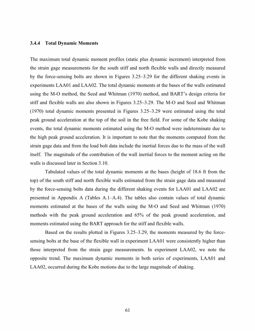
61
3.4.4 Total Dynamic Moments
The maximum total dynamic moment profiles (static plus dynamic increment) interpreted from
the strain gage measurements for the south stiff and north flexible walls and directly measured
by the force-sensing bolts are shown in Figures 3.25–3.29 for the different shaking events in
experiments LAA01 and LAA02. The total dynamic moments at the bases of the walls estimated
using the M-O method, the Seed and Whitman (1970) method, and BART’s design criteria for
stiff and flexible walls are also shown in Figures 3.25–3.29. The M-O and Seed and Whitman
(1970) total dynamic moments presented in Figures 3.25–3.29 were estimated using the total
peak ground acceleration at the top of the soil in the free field. For some of the Kobe shaking
events, the total dynamic moments estimated using the M-O method were indeterminate due to
the high peak ground acceleration. It is important to note that the moments computed from the
strain gage data and from the load bolt data include the inertial forces due to the mass of the wall
itself. The magnitude of the contribution of the wall inertial forces to the moment acting on the
walls is discussed later in Section 3.10.
Tabulated values of the total dynamic moments at the bases (height of 18.6 ft from the
top) of the south stiff and north flexible walls estimated from the strain gage data and measured
by the force-sensing bolts data during the different shaking events for LAA01 and LAA02 are
presented in Appendix A (Tables A.1–A.4). The tables also contain values of total dynamic
moments estimated at the bases of the walls using the M-O and Seed and Whitman (1970)
methods with the peak ground acceleration and 65% of the peak ground acceleration, and
moments estimated using the BART approach for the stiff and flexible walls.
Based on the results plotted in Figures 3.25–3.29, the moments measured by the force-
sensing bolts at the base of the flexible wall in experiment LAA01 were consistently higher than
those interpreted from the strain gage measurements. In experiment LAA02, we note the
opposite trend. The maximum dynamic moments in both series of experiments, LAA01 and
LAA02, occurred during the Kobe motions due to the large magnitude of shaking.

62
Loma Prieta-1LAA01
0
50
100
150
200
0 50 100x106
Total Dynamic Moment (lb-in)
Z (in
)
Meas. SG-StiffMeas. SG-FlexibleS&W EstimateBART-StiffBART-FlexibleMeas. LB-StiffMeas. LB-FlexibleM-O Estimate
Loma Prieta-SC-1LAA02
0
50
100
150
200
0 50 100x106
Total Dynamic Moment (lb-in)
Z (in
)
Meas. SG-StiffMeas. SG-FlexibleM-O EstimateS&W EstimateBART-StiffBART-FlexibleMeas. LB-StiffMeas. LB-Flexible
Loma Prieta-2LAA01
0
50
100
150
200
0 50 100x106
Total Dynamic Moment (lb-in)
Z (in
)
Meas. SG-StiffMeas. SG-FlexibleS&W EstimateBART-StiffBART-FlexibleMeas. LB-StiffMeas. LB-FlexibleM-O Estimate
Fig. 3.25 Maximum total dynamic moment profiles measured by strain gages and force-sensing bolts and estimated using M-O, Seed and Whitman (1970), and BART’s methods on stiff and flexible walls for Loma Prieta-1 and -2 for LAA01, and for Loma Prieta-SC-1 for LAA02.

63
KobeLAA01
0
50
100
150
200
0 50 100 150x106
Total Dynamic Moment (lb-in)Z
(in)
Meas. SG-Stiff
Meas. SG-Flexible
S&W Estimate
BART-Stiff
BART-Flexible
Meas. LB-Stiff
Meas. LB-Flexible
Kobe-PI-1LAA02
0
50
100
150
200
0 50 100 150x106
Total Dynamic Moment (lb-in)
Z (in
)
Meas. SG-StiffMeas. SG-FlexibleS&W EstimateM-O EstimateMeas. LB-StiffMeas. LB-FlexibleBART-StiffBART-Flexible
Kobe-PI-2LAA02
0
50
100
150
200
0 100x106
Total Dynamic Moment (lb-in)
Z (in
)
Meas. SG-Stiff
Meas. SG-Flexible
S&W EstimateBART-Stiff
BART-Flexible
Meas. LB-Stiff
Meas. LB-Flexible
Fig. 3.26 Maximum total dynamic moment profiles measured by strain gages and force-sensing bolts and estimated using M-O, Seed and Whitman (1970), and BART’s methods on stiff and flexible walls for Kobe during LAA01, and for Kobe-PI-1 and -2 for LAA02.
64
Loma Prieta-3LAA01
0
50
100
150
200
0 50 100x106
Total Dynamic Moment (lb-in)Z
(in)
Meas. SG-StiffMeas. SG-FlexibleS&W EstimateBART-StiffBART-FlexibleMeas. LB-StiffMeas. LB-FlexibleM-O Estimate
Loma Prieta-SC-2LAA02
0
50
100
150
200
0 50 100x106
Total Dynamic Moment (lb-in)
Z (in
)
Meas. SG-StiffMeas. SG-FlexibleS&W EstimateM-O EstimateMeas. LB-StiffMeas. LB-FlexibleBART-StiffBART-Flexible
Kocaeli-YPT060-2LAA02
0
50
100
150
200
0 50 100x106
Total Dynamic Moment (lb-in)
Z (in
)
Meas.SG-StiffMeas. SG-FlexibleM-O EstimateS&W EstimateBART-StiffBART-FlexibleMeas. LB-StiffMeas. LB-Flexible
Kocaeli-YPT060-3LAA02
0
50
100
150
200
0 50 100x106
Total Dynamic Moment (lb-in)
Z (in
)
Meas. SG-StiffMeas. SG-FlexibleM-O EstimateS&W EstimateBART-StiffBART-FlexibleMeas. LB-StiffMeas. LB-Flexible
Fig. 3.27 Maximum total dynamic moment profiles measured by strain gages and force-sensing bolts and estimated using M-O, Seed and Whitman (1970), and BART’s methods on stiff and flexible walls for Loma Prieta-3 for LAA01, and for Loma Prieta-SC-2, and Kocaeli-YPT060-1 and 2 for LAA02.

65
Kocaeli-YPT330-2LAA02
0
50
100
150
200
0 50 100x106
Total Dynamic Moment (lb-in)Z
(in)
Meas. SG-StiffMeas. SG-FlexibleM-O EstimateS&W EstimateBART-StiffBART-FlexibleMeas. LB-StiffMeas. LB-Flexible
Kobe-TAK090-1LAA02
0
50
100
150
200
0 100 200x106
Total Dynamic Moment (lb-in)
Z (in
)
Meas. SG-Stiff
Meas. SG-Flexible
S&W Estimate
BART-Stiff
BART-Flexible
Meas. LB-StiffMeas. LB-Flexible
Kobe-TAK090-2LAA02
0
50
100
150
200
0 100x106
Total Dynamic Moment (lb-in)
Z (in
)
Meas. SG-StiffMeas. SG-FlexibleS&W EstimateM-O EstimateMeas. LB-StiffMeas. LB-FlexibleBART-StiffBART-Flexible
Loma Prieta-WVC270LAA02
0
50
100
150
200
0 50 100x106
Total Dynamic Moment (lb-in)
Z (in
)
Meas. SG-StiffMeas. SG-FlexibleS&W EstimateBART-StiffBART-FlexibleM-O EstimateMeas. LB-StiffMeas. LB-Flexible
Fig. 3.28 Maximum total dynamic moment profiles measured by strain gages and force-sensing bolts and estimated using M-O, Seed and Whitman (1970), and BART’s methods on stiff and flexible walls for Kocaeli-YPT330-2, Kobe-TAK090-1 and 2 and Loma Prieta-WVC270 for LAA02.

66
Kocaeli-YPT330-3LAA02
0
50
100
150
200
0 50 100x106
Total Dynamic Moment (lb-in)
Z (in
)
Meas. SG-StiffMeas. SG-FlexibleS&W EstimateBART-StiffBART-FlexibleM-O EstimateMeas. LB-StiffMeas. LB-Flexible
Fig. 3.29 Maximum total dynamic moment profiles measured by strain gages and force-sensing bolts and estimated using M-O, Seed and Whitman (1970), and BART’s methods on stiff and flexible walls for Kocaeli-YPT330-3 for LAA02.
Tables 3.9–3.16 present computed moments based on the M-O, Seed and Whitman
(1970), and BART methods as a ratio in percent of the maximum total dynamic moments
interpreted from the strain gage data on the stiff and the flexible walls for the different shaking
events for LAA01 and LAA02. M-O and Seed and Whitman (1970) moment estimates are
calculated with peak and 65% of the peak ground accelerations measured at the top of the soil in
the free field. Note that Seed and Whitman seem to recommend 85% rather than the more
commonly assumed 65% of the peak ground acceleration. Whenever the total dynamic moment
estimates underestimate the measured maximum total dynamic moments, the corresponding
values are presented in bold red.

67
Table 3.9 Ratio of computed total dynamic moment to maximum total dynamic moments interpreted from strain gage data at base of south stiff wall during Loma Prieta-1, 2, and 3, and Kobe shaking events for LAA01.
Moment Estimates / Measured Moments Loma Prieta-1 Loma Prieta-2 Kobe Loma Prieta-3
BART Estimates 130% 122% 113% 128%
M-O Method with amax 102% 96% INDET 107%
M-O Method with 65% amax 67% 63% 61% 66%
Seed and Whitman (1970) Method with amax
127% 120% 106% 125%
Seed and Whitman (1970) Method with 65% amax
95% 89% 76% 92%
Table 3.10 Ratio of computed total dynamic moment to maximum total dynamic moments interpreted from strain gage data at base of north flexible wall during Loma Prieta-1, 2, and 3, and Kobe shaking events for LAA01.
Moment Estimates / Measured Moments Loma Prieta-1 Loma Prieta-2 Kobe Loma Prieta-3
BART Estimates 122 118 129 121
M-O Method with amax 156 150 INDET 164
M-O Method with 65% amax 102 99 111 102
Seed and Whitman (1970) Method with amax
194 188 193 192
Seed and Whitman (1970) Method with 65% amax
144 140 139 142

68
Table 3.11 Ratio of computed total dynamic moment to maximum total dynamic moments interpreted from strain gage data at base of south stiff wall during Loma Prieta-SC-1, Kobe-PI-1, Kobe-PI-2, and Loma Prieta-SC-2 shaking events for LAA02.
Moment Estimates / Measured Moments Loma Prieta-SC-1 Kobe-PI-1 Kobe-PI-2 Loma Prieta-SC-2
BART Estimates 138% 99% 114% 137%
M-O Method with amax 101% 114% INDET. 110%
M-O Method with 65% amax 70% 52% 61% 70%
Seed and Whitman (1970) Method with amax
139% 100% 113% 141%
Seed and Whitman (1970) Method with 65% amax
103% 72% 80% 104%
Table 3.12 Ratio of computed total dynamic moment estimates to maximum total dynamic moments interpreted from strain gage data at base of north flexible wall during Loma Prieta-SC-1, Kobe-PI-1, Kobe-PI-2, and Loma Prieta-SC-2 shaking events for LAA02.
Moment Estimates / Measured Moments Loma Prieta-SC-1 Kobe-PI-1 Kobe-PI-2 Loma Prieta-SC-2
BART Estimates 99% 81% 91% 98%
M-O Method with amax 119% 150% INDET. 128%
M-O Method with 65% amax 83% 68% 78% 82%
Seed and Whitman (1970) Method with amax
164% 131% 144% 164%
Seed and Whitman (1970) Method with 65% amax
122% 94% 103% 121%

69
Table 3.13 Ratio of computed total dynamic moment to maximum total dynamic moments interpreted from strain gage data at base of south stiff wall during Kocaeli-YPT060-2, Kocaeli-YPT060-3, Kocaeli-YPT330-2, and Kobe-TAK090-1 shaking events for LAA02.
Moment Estimates / Measured Moments
Kocaeli-
YPT060-2 Kocaeli-
YPT060-3 Kocaeli-
YPT330-2 Kobe-
TAK090-1
BART Estimates 197% 155% 177% 120%
M-O Method with amax 126% 109% 123% INDET.
M-O Method with 65% amax 102% 80% 91% 66%
Seed and Whitman (1970) Method with amax
187% 157% 178% 115%
Seed and Whitman (1970) Method with 65% amax
146% 118% 134% 81%
Table 3.14 Ratio of computed total dynamic moment to maximum total dynamic moments interpreted from strain gage data at base of north flexible wall during Kocaeli-YPT060-2, Kocaeli-YPT060-3, Kocaeli-YPT330-2, and Kobe-TAK090-1 shaking events for LAA02.
Moment Estimates / Measured Moments
Kocaeli-
YPT060-2 Kocaeli-
YPT060-3 Kocaeli-
YPT330-2 Kobe-
TAK090-1
BART Estimates 142% 151% 143% 108%
M-O Method with amax 153% 175% 164% INDET.
M-O Method with 65% amax 124% 128% 120% 94%
Seed and Whitman (1970) Method with amax
228% 252% 237% 162%
Seed and Whitman (1970) Method with 65% amax
177% 190% 179% 114%

70
Table 3.15 Ratio of computed total dynamic moment to maximum total dynamic moments interpreted from strain gage data at base of south stiff wall during Kobe-TAK090-2, Loma Prieta-WVC270, and Loma Kocaeli-YPT330-3 shaking events for LAA02.
Moment Estimates / Measured Moments Kobe-TAK090-2 Loma Prieta-WVC270 Kocaeli-YPT330-3
BART Estimates 115% 177% 169%
M-O Method with amax 112% 115% 119%
M-O Method with 65% amax 60% 91% 90%
Seed and Whitman (1970) Method with amax
118% 173% 177%
Seed and Whitman (1970) Method with 65% amax
85% 133% 134%
Table 3.16 Ratio of computed total dynamic moment to maximum total dynamic moments interpreted from strain gage data at base of north flexible wall during Kobe-TAK090-2, Loma Prieta-WVC270, and Loma Kocaeli-YPT330-3 shaking events for LAA02.
Moment Estimates / Measured Moments Kobe-TAK090-2 Loma Prieta-WVC270 Kocaeli-YPT330-3
BART Estimates 108% 111% 113%
M-O Method with amax 170% 121% 133%
M-O Method with 65% amax 90% 95% 100%
Seed and Whitman (1970) Method with amax
178% 181% 197%
Seed and Whitman (1970) Method with 65% amax
129% 140% 150%
Tables 3.9–3.16 show that the M-O and Seed and Whitman (1970) methods used with the
total peak ground accelerations typically overestimate the maximum measured total dynamic
moment values. The ratio of the observed maximum total dynamic moments to the estimated
total dynamic moments appears to be a function of the flexibility of the wall, the magnitude of

71
shaking, and the density of the sand backfill. The overestimate is not as large for stiff wall, and a
large magnitude of shaking with relatively loose backfill.
Using 65% of the peak ground accelerations measured at the top of the soil in the free
field, the M-O method generally underestimates the maximum observed total dynamic moments,
especially on the stiff wall. Using 65% of the peak ground accelerations measured at the top of
the soil in the free field, the Seed and Whitman (1970) method slightly underestimates the
moments measured at the base of the stiff wall in experiment LAA01. In experiment LAA02 the
same approach generally overestimates the moments due to the higher soil density except for the
moments on the stiff wall during the Kobe shaking events.
Overall, the maximum observed total dynamic moments for the stiff wall are generally
adequately estimated or overestimated by the BART design criteria for all shaking events.
However, the BART design criteria apparently underestimate the maximum total dynamic
moments on the flexible wall for all the shaking events during LAA01, and the Loma Prieta-SC-
1 and 2 and Kobe-PI-1 and 2 shaking events during LAA02, although this typically occurs only
in one cycle of loading as shown later.
3.4.5 Dynamic Moment Increments
Dynamic moment increments were determined by applying a moving average filter to the
moment time series directly measured by the force-sensing bolts and interpreted from the strain
gage data. The moving average filter determines the static trend for each moment time series;
deducing this trend from the corresponding total (static plus dynamic) moment time series results
in a dynamic moment increment time series. The procedure outlined in Section 3.4.1 (Analysis
Procedure and Assumptions) for determining the maximum total dynamic moments at the bases
of the south stiff and north flexible walls and the maximum total dynamic moment profiles from
the strain gage data were applied to determine the maximum dynamic moment increment values
and profiles.
The maximum dynamic increment moment distributions interpreted from the strain gage
measurements for the south stiff and north flexible walls and those directly measured by the
force-sensing bolts are shown in Figures 3.30–3.34 for the different shaking events in
experiments LAA01 and LAA02. The dynamic moment increments at the bases of the walls
estimated using the M-O method, the Seed and Whitman (1970) method, and BART’s design
72
criteria for stiff and flexible walls are also shown in Figures 3.30–3.34. The M-O and Seed and
Whitman (1970) dynamic moment increments presented in Figures 3.30–3.34 were estimated
using the total peak ground acceleration at the top of the soil in the free field. While the values
of the maximum dynamic moment increment still contain the moments due to the wall inertial
forces, they eliminate the increment in static moment on the wall as a result of compaction of the
backfill. Thus, they provide a more representative measure of the actual dynamic loading on the
walls.
The plots in Figures 3.30–3.34 show that the maximum dynamic moment increments at
the bases of the south stiff and north flexible walls generally tend to be overestimated by the M-
O and Seed and Whitman methods. Similarly, the BART design criteria tend to overestimate the
measured dynamic moment increments at the bases of the walls, except for the first Kobe event
in both experiments when the BART design criteria slightly underestimate the observed
maximum dynamic moment increment.
Tabulated values of the computed dynamic moment increments at the bases (height of
18.6 ft from the top) of the south stiff and north flexible walls as interpreted from the strain gage
data and measured by the force-sensing bolts during the different shaking events for LAA01 and
LAA02 are presented in Appendix A (Table A.9–A.10). As before, the dynamic moment
increments estimated at the bases of the walls using the M-O and Seed and Whitman (1970)
methods with the peak ground acceleration and 65% of the peak ground acceleration and with
BART design criteria are also included for comparison.

73
Loma Prieta-1LAA01
0
50
100
150
200
0 40 80x106
Dynamic Moment Increment (lb-in)
Z (in
)
Meas. SG-StiffMeas. SG-FlexibleS&W EstimateBART-StiffBART-FlexibleMeas. LB-StiffMeas. LB-FlexibleM-O Estimate
Loma Prieta-SC-1LAA02
0
50
100
150
200
0 40 80x106
Dynamic Moment Increment (lb-in)
Z (in
)
Meas. SG-StiffMeas. SG-FlexibleS&W EstimateBART-StiffBART-FlexibleMeas. LB-StiffMeas. LB-FlexibleM-O Estimate
Loma Prieta-2LAA01
0
50
100
150
200
0 40 80x106
Dynamic Moment Increment (lb-in)
Z (in
)
Meas. SG-StiffMeas. SG-FlexibleS&W EstimateBART-StiffBART-FlexibleMeas. LB-StiffMeas. LB-FlexibleM-O Estimate
Fig. 3.30 Maximum dynamic moment increment profiles measured by strain gages and force-sensing bolts and estimated using M-O, Seed and Whitman (1970), and BART’s methods on stiff and flexible walls for Loma Prieta-1 and 2 for LAA01, and for Loma Prieta-SC-1 for LAA02.
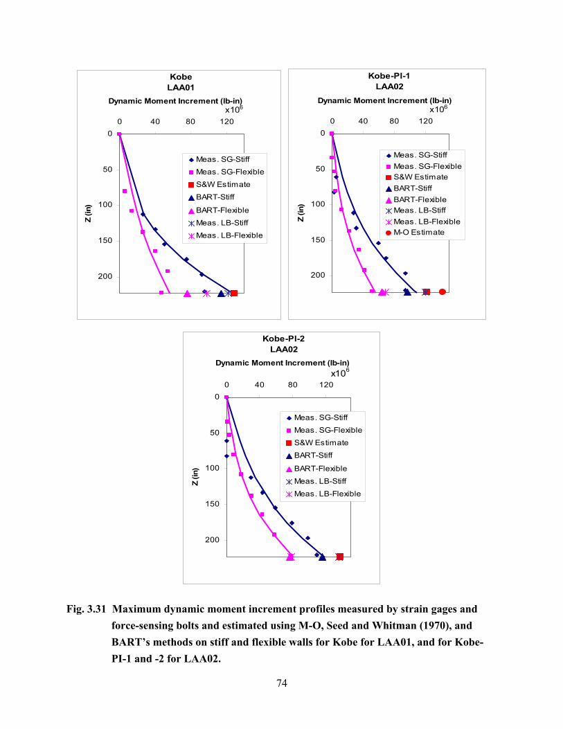
74
KobeLAA01
0
50
100
150
200
0 40 80 120x106
Dynamic Moment Increment (lb-in)
Z (in
)
Meas. SG-StiffMeas. SG-Flexible
S&W Estimate
BART-Stiff
BART-Flexible
Meas. LB-StiffMeas. LB-Flexible
Kobe-PI-1LAA02
0
50
100
150
200
0 40 80 120x106
Dynamic Moment Increment (lb-in)
Z (in
)
Meas. SG-StiffMeas. SG-FlexibleS&W EstimateBART-StiffBART-FlexibleMeas. LB-StiffMeas. LB-FlexibleM-O Estimate
Kobe-PI-2LAA02
0
50
100
150
200
0 40 80 120x106
Dynamic Moment Increment (lb-in)
Z (in
)
Meas. SG-Stiff
Meas. SG-Flexible
S&W Estimate
BART-Stiff
BART-Flexible
Meas. LB-Stiff
Meas. LB-Flexible
Fig. 3.31 Maximum dynamic moment increment profiles measured by strain gages and force-sensing bolts and estimated using M-O, Seed and Whitman (1970), and BART’s methods on stiff and flexible walls for Kobe for LAA01, and for Kobe-PI-1 and -2 for LAA02.
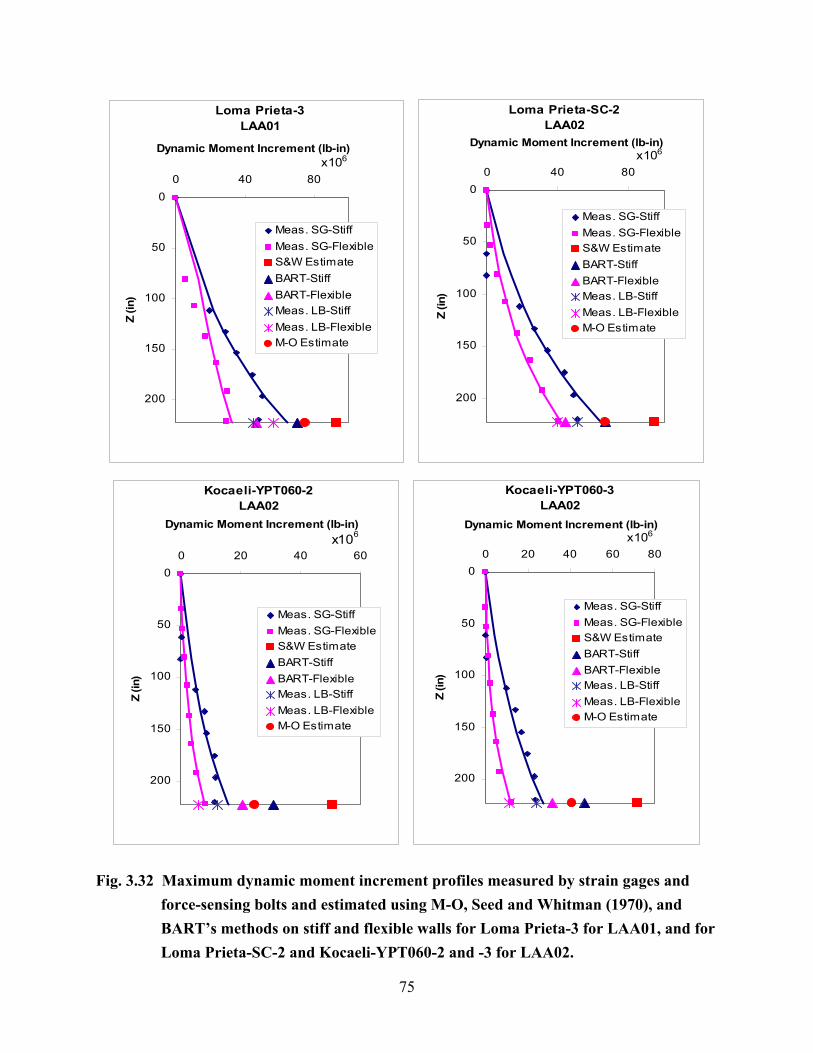
75
Loma Prieta-3LAA01
0
50
100
150
200
0 40 80x106
Dynamic Moment Increment (lb-in)Z
(in)
Meas. SG-StiffMeas. SG-FlexibleS&W EstimateBART-StiffBART-FlexibleMeas. LB-StiffMeas. LB-FlexibleM-O Estimate
Loma Prieta-SC-2LAA02
0
50
100
150
200
0 40 80x106
Dynamic Moment Increment (lb-in)
Z (in
)
Meas. SG-StiffMeas. SG-FlexibleS&W EstimateBART-StiffBART-FlexibleMeas. LB-StiffMeas. LB-FlexibleM-O Estimate
Kocaeli-YPT060-2LAA02
0
50
100
150
200
0 20 40 60x106
Dynamic Moment Increment (lb-in)
Z (in
)
Meas. SG-StiffMeas. SG-FlexibleS&W EstimateBART-StiffBART-FlexibleMeas. LB-StiffMeas. LB-FlexibleM-O Estimate
Kocaeli-YPT060-3LAA02
0
50
100
150
200
0 20 40 60 80x106
Dynamic Moment Increment (lb-in)
Z (in
)
Meas. SG-StiffMeas. SG-FlexibleS&W EstimateBART-StiffBART-FlexibleMeas. LB-StiffMeas. LB-FlexibleM-O Estimate
Fig. 3.32 Maximum dynamic moment increment profiles measured by strain gages and force-sensing bolts and estimated using M-O, Seed and Whitman (1970), and BART’s methods on stiff and flexible walls for Loma Prieta-3 for LAA01, and for Loma Prieta-SC-2 and Kocaeli-YPT060-2 and -3 for LAA02.

76
Kocaeli-YPT330-2LAA02
0
50
100
150
200
0 20 40 60 80x106
Dynamic Moment Increment (lb-in)Z
(in)
Meas. SG-StiffMeas. SG-FlexibleS&W EstimateBART-StiffBART-FlexibleMeas. LB-StiffMeas. LB-FlexibleM-O Estimate
Kobe-TAK090-1LAA02
0
50
100
150
200
0 40 80 120 160x106
Dynamic Moment Increment (lb-in)
Z (in
)
Meas. SG-Stiff
Meas. SG-Flexible
S&W Estimate
BART-Stiff
BART-Flexible
Meas. LB-Stiff
Meas. LB-Flexible
Kobe-TAK090-2LAA02
0
50
100
150
200
0 40 80 120x106
Dynamic Moment Increment (lb-in)
Z (in
)
Meas. SG-StiffMeas. SG-FlexibleS&W EstimateBART-StiffBART-FlexibleMeas. LB-StiffMeas. LB-FlexibleM-O Estimate
Loma Prieta-WVC270LAA02
0
50
100
150
200
0 20 40 60x106
Dynamic Moment Increment (lb-in)
Z (in
)
Meas. SG-StiffMeas. SG-FlexibleS&W EstimateBART-StiffBART-FlexibleMeas. LB-StiffMeas. LB-FlexibleM-O Estimate
Fig. 3.33 Maximum dynamic moment increment profiles measured by strain gages and force-sensing bolts and estimated using M-O, Seed and Whitman (1970), and BART’s methods on stiff and flexible walls for Kocaeli-YPT330-2, Kobe-TAK090-1 and -2 and Loma Prieta-WVC270 for LAA02.

77
Kocaeli-YPT330-3LAA02
0
50
100
150
200
0 20 40 60 80x106
Dynamic Moment Increment (lb-in)
Z (in
)
Meas. SG-StiffMeas. SG-FlexibleS&W EstimateBART-StiffBART-FlexibleMeas. LB-StiffMeas. LB-FlexibleM-O Estimate
Fig. 3.34 Maximum dynamic moment increment profiles measured by strain gages and force-sensing bolts and estimated using M-O, Seed and Whitman (1970, and BART’s methods on stiff and flexible walls for Kocaeli-YPT330-3 for LAA02.
Tables 3.17–3.24 present the M-O, Seed and Whitman (1970), and BART’s dynamic
moment increments estimates as a ratio in percent of the maximum dynamic moment increments
interpreted from the strain gage data on the stiff and the flexible walls for the different shaking
events for LAA01 and LAA02. M-O and Seed and Whitman (1970) moment estimates are
calculated with peak and 65% of the peak ground accelerations measured at the top of the soil in
the free field. Whenever the dynamic moment increment estimates underestimate the measured
dynamic moment increments, the corresponding values are presented in bold red in Tables 3.17–
3.24.

78
Table 3.17 Ratio of computed dynamic moment increment to maximum dynamic moment increment interpreted from strain gage data at base of south stiff wall during Loma Prieta-1, 2, and 3, and Kobe shaking events for LAA01.
Moment Estimates / Measured Moments Loma Prieta-1 Loma Prieta-2 Kobe Loma Prieta-3
BART Estimates 105% 97% 89% 109%
M-O Method with amax 104% 96% INDET. 116%
M-O Method with 65% amax 50% 47% 47% 53%
Seed and Whitman (1970) Method with amax
141% 132% 100% 143%
Seed and Whitman (1970) Method with 65% amax
92% 86% 65% 93%
Table 3.18 Ratio of computed dynamic moment increment to maximum dynamic moment increment interpreted from strain gage data at the base of north flexible wall during Loma Prieta-1, 2, and 3, and Kobe shaking events for LAA01.
Moment Estimates / Measured Moments Loma Prieta-1 Loma Prieta-2 Kobe Loma Prieta-3
BART Estimates 126% 126% 135% 143%
M-O Method with amax 188% 187% INDET. 228%
M-O Method with 65% amax 91% 91% 107% 104%
Seed and Whitman (1970) Method with amax
256% 256% 227% 282%
Seed and Whitman (1970) Method with 65% amax
166% 166% 148% 183%

79
Table 3.19 Ratio of computed dynamic moment increment to maximum dynamic moment increment interpreted from strain gage data at base of south stiff wall during Loma Prieta-SC-1, Kobe-PI-1, Kobe-PI-2, and Loma Prieta-SC-2 shaking events for LAA02.
Moment Estimates / Measured Moments Loma Prieta-SC-1 Kobe-PI-1 Kobe-PI-2 Loma Prieta-SC-2
BART Estimates 116% 89% 97% 103%
M-O Method with amax 106% 131% INDET. 104%
M-O Method with 65% amax 55% 45% 51% 50%
Seed and Whitman (1970) Method with amax
170% 112% 115% 146%
Seed and Whitman (1970) Method with 65% amax
110% 73% 75% 95%
Table 3.20 Ratio of computed dynamic moment increment to maximum dynamic moment increment interpreted from strain gage data at base of north flexible wall during Loma Prieta-SC-1, Kobe-PI-1, Kobe-PI-2, and Loma Prieta-SC-2 shaking events for LAA02.
Moment Estimates / Measured Moments Loma Prieta-SC-1 Kobe-PI-1 Kobe-PI-2 Loma Prieta-SC-2
BART Estimates 145% 116% 95% 106%
M-O Method with amax 199% 257% INDET. 159%
M-O Method with 65% amax 102% 89% 75% 76%
Seed and Whitman (1970) Method with amax
319% 219% 169% 224%
Seed and Whitman (1970) Method with 65% amax
207% 143% 110% 146%
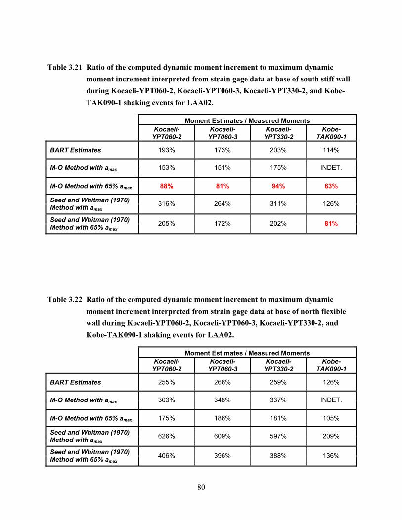
80
Table 3.21 Ratio of the computed dynamic moment increment to maximum dynamic moment increment interpreted from strain gage data at base of south stiff wall during Kocaeli-YPT060-2, Kocaeli-YPT060-3, Kocaeli-YPT330-2, and Kobe-TAK090-1 shaking events for LAA02.
Moment Estimates / Measured Moments
Kocaeli-
YPT060-2 Kocaeli-
YPT060-3 Kocaeli-
YPT330-2 Kobe-
TAK090-1
BART Estimates 193% 173% 203% 114%
M-O Method with amax 153% 151% 175% INDET.
M-O Method with 65% amax 88% 81% 94% 63%
Seed and Whitman (1970) Method with amax
316% 264% 311% 126%
Seed and Whitman (1970) Method with 65% amax
205% 172% 202% 81%
Table 3.22 Ratio of the computed dynamic moment increment to maximum dynamic moment increment interpreted from strain gage data at base of north flexible wall during Kocaeli-YPT060-2, Kocaeli-YPT060-3, Kocaeli-YPT330-2, and Kobe-TAK090-1 shaking events for LAA02.
Moment Estimates / Measured Moments
Kocaeli-
YPT060-2 Kocaeli-
YPT060-3 Kocaeli-
YPT330-2 Kobe-
TAK090-1
BART Estimates 255% 266% 259% 126%
M-O Method with amax 303% 348% 337% INDET.
M-O Method with 65% amax 175% 186% 181% 105%
Seed and Whitman (1970) Method with amax
626% 609% 597% 209%
Seed and Whitman (1970) Method with 65% amax
406% 396% 388% 136%

81
Table 3.23 Ratio of computed dynamic moment increment to maximum dynamic moment increment interpreted from strain gage data at base of south stiff wall during Kobe-TAK090-2, Loma Prieta-WVC270, and Loma Kocaeli-YPT330-3 shaking events for LAA02.
Moment Estimates / Measured Moments Kobe-TAK090-2 Loma Prieta-WVC270 Kocaeli-YPT330-3
BART Estimates 103% 227% 250%
M-O Method with amax 127% 183% 210%
M-O Method with 65% amax 51% 104% 116%
Seed and Whitman (1970) Method with amax
136% 371% 396%
Seed and Whitman (1970) Method with 65% amax
88% 241% 257%
Table 3.24 Ratio of computed dynamic moment increment to maximum dynamic moment increment interpreted from strain gage data at base of north flexible wall during Kobe-TAK090-2, Loma Prieta-WVC270, and Loma Kocaeli-YPT330-3 shaking events for LAA02.
Moment Estimates / Measured Moments Kobe-TAK090-2 Loma Prieta-WVC270 Kocaeli-YPT330-3
BART Estimates 146% 239% 250%
M-O Method with amax 269% 290% 315%
M-O Method with 65% amax 109% 164% 174%
Seed and Whitman (1970) Method with amax
289% 586% 594%
Seed and Whitman (1970) Method with 65% amax
187% 380% 385%
Tables 3.17–3.24 show that M-O and Seed and Whitman (1970) methods used with the
total peak ground accelerations overestimate the maximum observed dynamic moment
increments. Again, we note that the ratio of the observed maximum dynamic moment increments
to the computed values appears to be a function of the flexibility of the wall, the magnitude of

82
shaking, and the density of the sand backfill, with the magnitude of the overestimate being lower
for the stiff wall.
Using 65% of the peak ground accelerations measured at the top of the soil in the free
field, the M-O method generally underestimates the maximum observed dynamic moment
increments, especially on the stiff wall, while the Seed and Whitman (1970) method adequately
estimates if not overestimates the measured dynamic moment increments. BART design criteria
generally overestimate the dynamic moment increments on the stiff and the flexible walls.
3.5 SHEAR DISTRIBUTIONS
3.5.1 Analysis Procedure and Assumptions
Maximum total dynamic shear profiles were obtained by differentiating the maximum total
dynamic moment profiles interpreted from the strain gage measurements. Since the best fit for
the total dynamic moments interpreted from the strain gages is a cubic polynomial fit of the form
M = a*z3 + b*z, the total dynamic shear profiles have a quadratic form: V = 3a*z2 + b. It is
important to note that due to the form of the best-fit equation for the observed moment
distribution, the equation for shear distribution gives a non-zero intercept and hence a shear at
the top of the wall that is physically impossible. Thus, only the computed value of maximum
shear at the base should be considered as fully representative.
The computed total dynamic shear profiles and shear values at the bases of the south stiff
and north flexible walls are compared to the estimated shear values using M-O and Seed and
Whitman (1970) using the peak ground acceleration and 65% of the peak ground acceleration
measured at the top of the soil in the free field for the stiff and flexible walls. Total dynamic
shear estimates using the BART design criteria are also presented. BART design criteria for stiff
walls assume at-rest (Ko) earth pressures for static loads and 1.5 times the M-O inverted
triangular pressure increment for seismic loads. For flexible walls, BART design criteria assume
active earth pressures for static loads and M-O inverted triangular pressure increment for seismic
loads. For both stiff and flexible walls, half the peak ground accelerations measured at the top of
the soil in the free field were used with the BART design criteria.

83
3.5.2 Total Dynamic Shear Distributions
Tabulated values of the computed total dynamic shear at the bases (height of 18.6 ft from the
top) of the south stiff and north flexible walls interpreted from the strain gage measurements
during the different shaking events in experiments LAA01 and LAA02 are presented in
Appendix A (Tables A.5–A.8). The total dynamic shear values estimated at the bases of the walls
using the M-O and Seed and Whitman (1970) methods with the peak ground acceleration and
65% of the peak ground acceleration, and using the BART criteria are also presented for
comparison.
The maximum total dynamic shear distributions interpreted from the strain gage
measurements are plotted in Figures 3.35–3.39 for the different shaking events in experiments
LAA01 and LAA02. The plots show that the shear profiles interpreted from the strain gage
measurements on the south stiff wall are generally higher than those on the north flexible wall.
Shear estimates at the bases of the stiff and the flexible walls obtained using the M-O and Seed
and Whitman methods tend to overestimate the shear values interpreted from the strain gage
measurements, except for Kobe-PI-1, LAA02. The shear values interpreted from the strain gage
measurements at the bases of the stiff and the flexible walls are generally adequately estimated
by the BART design criteria for all the shaking events except for Loma Prieta-SC-1 and 2 and
some of the Kobe shaking events during LAA02. This result is consistent with the moment
distribution results as would be expected, due to the functional relationship already mentioned.
Also, these values again include the shear due to motion of the wall itself as already discussed.

84
Loma Prieta-1LAA01
0
50
100
150
200
0 0.4 0.8 1.2x10⁶
Total Dynamic Shear (lb)Z
(in)
SGs-Stiff
SGs-Flexible
S&W Estimate
BART-Stiff
BART-Flexible
M-O Estimate
Loma Prieta-SC-1LAA02
0
50
100
150
200
0 0.4 0.8 1.2x10⁶
Total Dynamic Shear (lb)
Z (in
)
SGs-Stiff
SGs-Flexible
S&W Estimate
BART-Stiff
BART-Flexible
M-O Estimate
Loma Prieta-2LAA01
0
50
100
150
200
0 0.4 0.8 1.2x10⁶
Total Dynamic Shear (lb)
Z (in
)
SGs-Stiff
SGs-Flexible
S&W Estimate
BART-Stiff
BART-Flexible
M-O Estimate
Fig. 3.35 Maximum total dynamic shear profiles interpreted from strain gage measurements and estimated using M-O, Seed and Whitman (1970), and BART’s methods on stiff and flexible walls for Loma Prieta-1 and 2 for LAA01, and for Loma Prieta-SC-1 for LAA02.
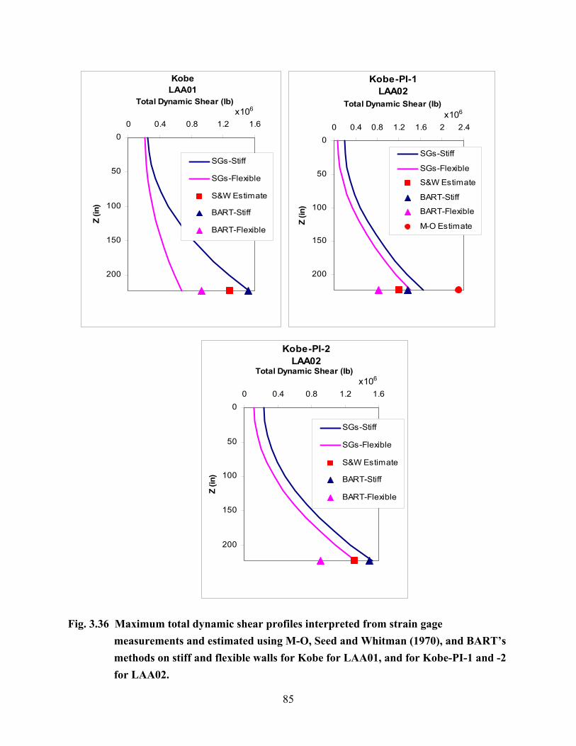
85
KobeLAA01
0
50
100
150
200
0 0.4 0.8 1.2 1.6x10⁶
Total Dynamic Shear (lb)Z
(in)
SGs-Stiff
SGs-Flexible
S&W Estimate
BART-Stiff
BART-Flexible
Kobe-PI-1LAA02
0
50
100
150
200
0 0.4 0.8 1.2 1.6 2 2.4x10⁶
Total Dynamic Shear (lb)
Z (in
)
SGs-Stiff
SGs-Flexible
S&W Estimate
BART-Stiff
BART-Flexible
M-O Estimate
Kobe-PI-2LAA02
0
50
100
150
200
0 0.4 0.8 1.2 1.6x10⁶
Total Dynamic Shear (lb)
Z (in
)
SGs-Stiff
SGs-Flexible
S&W Estimate
BART-Stiff
BART-Flexible
Fig. 3.36 Maximum total dynamic shear profiles interpreted from strain gage measurements and estimated using M-O, Seed and Whitman (1970), and BART’s methods on stiff and flexible walls for Kobe for LAA01, and for Kobe-PI-1 and -2 for LAA02.

86
Loma Prieta-3LAA01
0
50
100
150
200
0 0.4 0.8 1.2x10⁶
Total Dynamic Shear (lb)Z
(in)
SGs-Stiff
SGs-Flexible
S&W Estimate
BART-Stiff
BART-Flexible
M-O Estimate
Loma Prieta-SC-2LAA02
0
50
100
150
200
0 0.4 0.8 1.2x10⁶
Total Dynamic Shear (lb)
Z (in
)
SGs-Stiff
SGs-Flexible
S&W Estimate
BART-Stiff
BART-Flexible
M-O Estimate
Kocaeli-YPT060-2LAA02
0
50
100
150
200
0 0.4 0.8x10⁶
Total Dynamic Shear (lb)
Z (in
)
SGs-Stiff
SGs-Flexible
S&W Estimate
BART-Stiff
BART-Flexible
M-O Estimate
Kocaeli-YPT060-3LAA02
0
50
100
150
200
0 0.4 0.8 1.2x10⁶
Total Dynamic Shear (lb)
Z (in
)
SGs-Stiff
SGs-Flexible
S&W Estimate
BART-Stiff
BART-Flexible
M-O Estimate
Fig. 3.37 Maximum total dynamic shear profiles interpreted from strain gage measurements and estimated using M-O, Seed and Whitman (1970), and BART’s methods on stiff and flexible walls for Loma Prieta-3 for LAA01, and for Loma Prieta-SC-2 and Kocaeli-YPT060-2 and 3 for LAA02.

87
Kocaeli-YPT330-2LAA02
0
50
100
150
200
0 0.4 0.8 1.2x10⁶
Total Dynamic Shear (lb)Z
(in)
SGs-Stiff
SGs-Flexible
S&W Estimate
BART-Stiff
BART-Flexible
M-O Estimate
Kobe-TAK090-1LAA02
0
50
100
150
200
0 0.4 0.8 1.2 1.6x10⁶
Total Dynamic Shear (lb)
Z (in
)
SGs-Stiff
SGs-Flexible
S&W Estimate
BART-Stiff
BART-Flexible
Kobe-TAK090-2LAA02
0
50
100
150
200
0 0.4 0.8 1.2 1.6x10⁶
Total Dynamic Shear (lb)
Z (in
)
SGs-Stiff
SGs-Flexible
S&W Estimate
BART-Stiff
BART-Flexible
M-O Estimate
Loma Prieta-WVC270LAA02
0
50
100
150
200
0 0.4 0.8x10⁶
Total Dynamic Shear (lb)
Z (in
)
SGs-Stiff
SGs-Flexible
S&W Estimate
BART-Stiff
BART-Flexible
M-O Estimate
Fig. 3.38 Maximum total dynamic shear profiles interpreted from strain gage measurements and estimated using M-O, Seed and Whitman (1970), and BART’s methods on stiff and flexible walls for Kocaeli-YPT330-2, Kobe-TAK090-1 and 2 and Loma Prieta-WVC270 for LAA02.

88
Kocaeli-YPT330-3LAA02
0
50
100
150
200
0 0.4 0.8x10⁶
Total Dynamic Shear (lb)
Z (in
)
SGs-Stiff
SGs-Flexible
S&W Estimate
BART-Stiff
BART-Flexible
M-O Estimate
Fig. 3.39 Maximum total dynamic shear profiles interpreted from strain gage measurements and estimated using M-O, Seed and Whitman (1970), and BART’s methods on stiff and flexible walls for Kocaeli-YPT330-3 for LAA02.
Tables 3.25–3.32 present the M-O, Seed and Whitman (1970), and BART shear estimates
at the bases of the stiff and the flexible walls as a percentage of the maximum shear values
interpreted from the strain gage data for the different shaking events for LAA01 and LAA02.
The M-O and Seed and Whitman (1970) shear estimates are calculated with peak and 65% of the
peak ground accelerations measured at the top of the soil in the free field. Whenever the total
dynamic shear estimates underestimate the maximum interpreted shear values, the corresponding
values are presented in bold red in Tables 3.25–3.32.
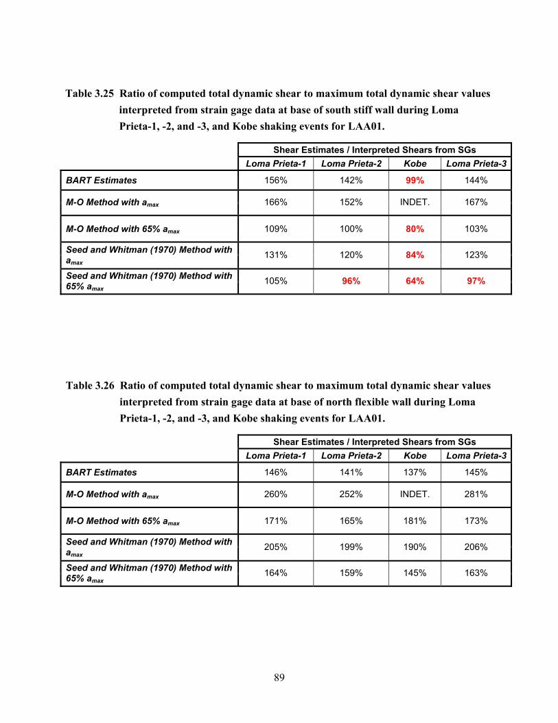
89
Table 3.25 Ratio of computed total dynamic shear to maximum total dynamic shear values interpreted from strain gage data at base of south stiff wall during Loma Prieta-1, -2, and -3, and Kobe shaking events for LAA01.
Shear Estimates / Interpreted Shears from SGs Loma Prieta-1 Loma Prieta-2 Kobe Loma Prieta-3
BART Estimates 156% 142% 99% 144%
M-O Method with amax 166% 152% INDET. 167%
M-O Method with 65% amax 109% 100% 80% 103%
Seed and Whitman (1970) Method with amax
131% 120% 84% 123%
Seed and Whitman (1970) Method with 65% amax
105% 96% 64% 97%
Table 3.26 Ratio of computed total dynamic shear to maximum total dynamic shear values interpreted from strain gage data at base of north flexible wall during Loma Prieta-1, -2, and -3, and Kobe shaking events for LAA01.
Shear Estimates / Interpreted Shears from SGs Loma Prieta-1 Loma Prieta-2 Kobe Loma Prieta-3
BART Estimates 146% 141% 137% 145%
M-O Method with amax 260% 252% INDET. 281%
M-O Method with 65% amax 171% 165% 181% 173%
Seed and Whitman (1970) Method with amax
205% 199% 190% 206%
Seed and Whitman (1970) Method with 65% amax
164% 159% 145% 163%

90
Table 3.27 Ratio of computed total dynamic shear to maximum total dynamic shear values interpreted from strain gage data at base of south stiff wall during Loma Prieta-SC-1, Kobe-PI-1, Kobe-PI-2, and Loma Prieta-SC-2 shaking events for LAA02.
Shear Estimates / Interpreted Shears from SGs Loma Prieta-SC-1 Kobe-PI-1 Kobe-PI-2 Loma Prieta-SC-2
BART Estimates 132% 82% 98% 141%
M-O Method with amax 128% 139% INDET. 157%
M-O Method with 65% amax 90% 64% 80% 100%
Seed and Whitman (1970) Method with amax
113% 73% 87% 125%
Seed and Whitman (1970) Method with 65% amax
90% 56% 65% 98%
Table 3.28 Ratio of computed total dynamic shear to maximum total dynamic shear values interpreted from strain gage data at base of north flexible wall during Loma Prieta-SC-1, Kobe-PI-1, Kobe-PI-2, and Loma Prieta-SC-2 shaking events for LAA02.
Shear Estimates / Interpreted Shears from SGs Loma Prieta-SC-1 Kobe-PI-1 Kobe-PI-2 Loma Prieta-SC-2
BART Estimates 81% 58% 69% 89%
M-O Method with amax 134% 162% #VALUE! 166%
M-O Method with 65% amax 94% 74% 92% 106%
Seed and Whitman (1970) Method with amax
118% 85% 100% 132%
Seed and Whitman (1970) Method with 65% amax
94% 65% 75% 103%
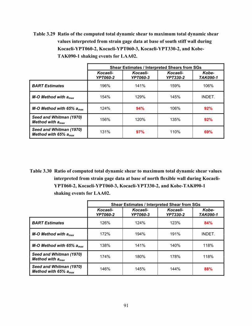
91
Table 3.29 Ratio of the computed total dynamic shear to maximum total dynamic shear values interpreted from strain gage data at base of south stiff wall during Kocaeli-YPT060-2, Kocaeli-YPT060-3, Kocaeli-YPT330-2, and Kobe-TAK090-1 shaking events for LAA02.
Shear Estimates / Interpreted Shears from SGs
Kocaeli-
YPT060-2 Kocaeli-
YPT060-3 Kocaeli-
YPT330-2 Kobe-
TAK090-1
BART Estimates 196% 141% 159% 106%
M-O Method with amax 154% 129% 145% INDET.
M-O Method with 65% amax 124% 94% 106% 92%
Seed and Whitman (1970) Method with amax
156% 120% 135% 92%
Seed and Whitman (1970) Method with 65% amax
131% 97% 110% 69%
Table 3.30 Ratio of computed total dynamic shear to maximum total dynamic shear values interpreted from strain gage data at base of north flexible wall during Kocaeli-YPT060-2, Kocaeli-YPT060-3, Kocaeli-YPT330-2, and Kobe-TAK090-1 shaking events for LAA02.
Shear Estimates / Interpreted Shear from SGs
Kocaeli-
YPT060-2 Kocaeli-
YPT060-3 Kocaeli-
YPT330-2 Kobe-
TAK090-1
BART Estimates 126% 124% 123% 84%
M-O Method with amax 172% 194% 191% INDET.
M-O Method with 65% amax 138% 141% 140% 118%
Seed and Whitman (1970) Method with amax
174% 180% 178% 118%
Seed and Whitman (1970) Method with 65% amax
146% 145% 144% 88%

92
Table 3.31 Ratio of computed total dynamic shear to maximum total dynamic shear values interpreted from strain gage data at base of south stiff wall during Kobe-TAK090-2, Loma Prieta-WVC270, and Loma Kocaeli-YPT330-3 shaking events for LAA02.
Shear Estimates / Interpreted Shears from SGs Kobe-TAK090-2 Loma Prieta-WVC270 Kocaeli-YPT330-3
BART Estimates 106% 161% 178%
M-O Method with amax 150% 130% 155%
M-O Method with 65% amax 79% 103% 117%
Seed and Whitman (1970) Method with amax
95% 131% 150%
Seed and Whitman (1970) Method with 65% amax
73% 108% 122%
Table 3.32 Ratio of computed total dynamic shear to maximum total dynamic shear values interpreted from strain gage data at base of north flexible wall during Kobe-TAK090-2, Loma Prieta-WVC270, and Loma Kocaeli-YPT330-3 shaking events for LAA02.
Shear Estimates / Interpreted Shear from SGs Kobe-TAK090-2 Loma Prieta-WVC270 Kocaeli-YPT330-3
BART Estimates 89% 100% 102%
M-O Method with amax 209% 141% 153%
M-O Method with 65% amax 111% 111% 115%
Seed and Whitman (1970) Method with amax
133% 142% 148%
Seed and Whitman (1970) Method with 65% amax
101% 117% 120%
Tables 3.25–3.32 show that the M-O and Seed and Whitman (1970) methods used with
the total peak ground accelerations generally overestimate the maximum total dynamic shear
values at the bases of the stiff and the flexible walls interpreted from the strain gage
measurements, except for some of the Kobe shaking events for LAA01 and LAA02. We note

93
that the ratio of the interpreted maximum total dynamic shear to the estimated total dynamic
shear is a function of the flexibility of the wall, the magnitude of shaking, and the density of the
sand backfill. Using 65% of the peak ground accelerations measured at the top of the soil in the
free field, the M-O and Seed and Whitman methods tend to underestimate the maximum
interpreted total shear on the stiff and the flexible walls for all the shaking events during LAA01
and for the Loma Prieta-SC-1 and some of the Kobe shaking events during LAA02.
The maximum observed dynamic shear values for the stiff wall are generally adequately
estimated, if not overestimated, by the BART design criteria for all shaking events. While it
appears that the BART design criteria underestimates the maximum total dynamic shear values
at the base of the flexible wall for the Loma Prieta-SC-1 and 2 and Kobe-PI-1 and 2 shaking
events during LAA02, it is important to note that the empirical curve fit used to interpret the
moment distributions significantly affects the computed values of shear. Hence, these data
should be used as a way of noting trends rather than absolute values.
3.6 LATERAL EARTH PRESSURES
3.6.1 Analysis Procedure and Assumptions
Ten Flexiforce sensors were mounted on all four walls to directly measure the seismically
induced lateral earth pressures at the locations shown in Figure 2.10 and Figure 2.11 for LAA01
and LAA02, respectively. Time series recorded by the Flexiforce sensors were filtered using a
first-order low-pass Butterworth filter with a prototype scale corner frequency of 22 Hz to reduce
noise. The Flexiforce sensors experienced drifting during both LAA01 and LAA02. As a result,
the original calibration factors could not be applied to the results. In order to interpret the
Flexiforce voltage records, we matched the static earth pressures recorded before and after each
shake to the corresponding static earth pressures interpreted from the strain gages, and we back-
calculated new calibration factors that take into account the drift of the response. These new
calibration factors were applied to interpret the total dynamic earth pressures recorded by the
Flexiforce sensors.
Seismically induced lateral earth pressure profiles were plotted for each wall by choosing
the time at which the maximum pressure occurred at the lowest Flexiforce sensor of each wall
and then plotting the pressures at all other Flexiforce sensors at that same time. Seismically

94
induced lateral earth pressure profiles were also interpreted from the strain gage responses by
double differentiating the cubic polynomial fits obtained for the total dynamic moment profiles.
For comparison, we present the total dynamic pressure distributions estimated by M-O and by
Seed and Whitman (1970) using the peak ground acceleration and 65% of the peak ground
acceleration measured at the top of the soil in the free field for the stiff and flexible walls. The
total dynamic pressure distributions estimated using the BART design criteria are also presented.
BART design criteria for stiff walls assume at-rest (Ko) earth pressures for static loads and 1.5
times the M-O inverted triangular pressure increment for seismic loads. For flexible walls,
BART design criteria assume active earth pressures for static loads and M-O inverted triangular
pressure increment for seismic loads. For both stiff and flexible walls, half the peak ground
accelerations measured at the top of the soil in the free field were used with the BART design
criteria.
3.6.2 Total Dynamic Earth Pressures and Comparisons
The seismically induced lateral earth pressure profiles directly measured by the Flexiforce
sensors on all four walls are shown in Figures 3.40–3.47 for the different shaking events for
LAA01 and LAA02. Based on Figures 3.40–3.47, we observe a consistent agreement between
the total dynamic earth pressures measured at the north and south walls of each structure. This is
an important observation in that it confirms that the models were not influenced by proximity to
the walls of the container and that the motions of the container were reasonably symmetrical.

95
Loma Prieta-1LAA01
0
50
100
150
200
0 2 4 6 8Pressure (psi)
Z (in
)
North Stiff South Stiff
Loma Prieta-1LAA01
0
50
100
150
200
0 2 4 6 8Pressure (psi)
Z (in
)North Flexible South Flexible
Loma Prieta-SC-1LAA02
0
50
100
150
200
0 2 4 6 8Pressure (psi)
Z (in
)
North Stiff South Stiff
Loma Prieta-SC-1LAA02
0
50
100
150
200
0 2 4 6 8Pressure (psi)
Z (in
)
North Flexible South Flexible
Fig. 3.40 Maximum total dynamic lateral earth pressure profiles measured by Flexiforce sensors on stiff and flexible walls during first Loma Prieta shaking events for LAA01 and LAA02.

96
Loma Prieta-2LAA01
0
50
100
150
200
0 2 4 6 8Pressure (psi)
Z (in
)
North Stiff South Stiff
Loma Prieta-2LAA01
0
50
100
150
200
0 2 4 6 8Pressure (psi)
Z (in
)North Flexible South Flexible
KobeLAA01
0
50
100
150
200
0 2 4 6 8Pressure (psi)
Z (in
)
North Stiff South Stiff
KobeLAA01
0
50
100
150
200
0 2 4 6 8Pressure (psi)
Z (in
)
North Flexible South Flexible
Fig. 3.41 Maximum total dynamic lateral earth pressure profiles measured by Flexiforce sensors on stiff and flexible walls during Loma Prieta -2 and Kobe shaking events for LAA01.

97
Kobe-PI-1LAA02
0
50
100
150
200
0 2 4 6 8Pressure (psi)
Z (in
)
North Stiff South Stiff
Kobe-PI-1LAA02
0
50
100
150
200
0 2 4 6 8Pressure (psi)
Z (in
)North Flexible South Flexible
Kobe-PI-2LAA02
0
50
100
150
200
0 2 4 6 8
Pressure (psi)
Z (in
)
North Stiff South Stiff
Kobe-PI-2LAA02
0
50
100
150
200
0 2 4 6 8Pressure (psi)
Z (in
)
North Flexible South Flexible
Fig. 3.42 Maximum total dynamic lateral earth pressure profiles measured by Flexiforce sensors on stiff and flexible walls during Kobe-PI-1 and -2 shaking events for LAA02.

98
Loma Prieta-3LAA01
0
50
100
150
200
0 2 4 6 8Pressure (psi)
Z (in
)
North Stiff South Stiff
Loma Prieta-3LAA01
0
50
100
150
200
0 2 4 6 8Pressure (psi)
Z (in
)North Flexible South Flexible
Loma Prieta-SC-2LAA02
0
50
100
150
200
0 2 4 6 8
Pressure (psi)
Z (in
)
North Stiff South Stiff
Loma-Prieta-SC-2LAA02
0
50
100
150
200
0 2 4 6 8Pressure (psi)
Z (in
)
North Flexible South Flexible
Fig. 3.43 Maximum total dynamic lateral earth pressure profiles measured by Flexiforce sensors on stiff and flexible walls during Loma Prieta-3 and Loma Prieta-SC-2 shaking events for LAA01 and LAA02, respectively.

99
Kocaeli-YPT060-2LAA02
0
50
100
150
200
0 2 4 6Pressure (psi)
Z (in
)
North Stiff South Stiff
Kocaeli-YPT060-2LAA02
0
50
100
150
200
0 2 4 6Pressure (psi)
Z (in
)North Flexible South Flexible
Kocaeli-YPT060-3LAA02
0
50
100
150
200
0 2 4 6 8Pressure (psi)
Z (in
)
North Stiff South Stiff
Kocaeli-YPT060-3LAA02
0
50
100
150
200
0 2 4 6 8Pressure (psi)
Z (in
)
North Flexible South Flexible
Fig. 3.44 Maximum total dynamic lateral earth pressure profiles measured by Flexiforce sensors on stiff and flexible walls during Kocaeli-YPT060-2 and -3 shaking events for LAA02.

100
Kocaeli-YPT330-2LAA02
0
50
100
150
200
0 2 4 6 8Pressure (psi)
Z (in
)
North Stiff South Stiff
Kocaeli-YPT330-2LAA02
0
50
100
150
200
0 5Pressure (psi)
Z (in
)North Flexible South Flexible
Kobe-TAK090-1LAA02
0
50
100
150
200
0 5 10 15Pressure (psi)
Z (in
)
North Stiff South Stiff
Kobe-TAK090-1LAA02
0
50
100
150
200
0 5 10 15Pressure (psi)
Z (in
)
North Flexible South Flexible
Fig. 3.45 Maximum total dynamic lateral earth pressure profiles measured by Flexiforce sensors on stiff and flexible walls during Kocaeli-YPT330-2 and Kobe-TAK090-1 shaking events for LAA02.
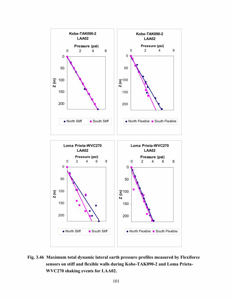
101
Kobe-TAK090-2LAA02
0
50
100
150
200
0 2 4 6Pressure (psi)
Z (in
)
North Stiff South Stiff
Kobe-TAK090-2LAA02
0
50
100
150
200
0 2 4 6Pressure (psi)
Z (in
)North Flexible South Flexible
Loma Prieta-WVC270LAA02
0
50
100
150
200
0 2 4 6 8Pressure (psi)
Z (in
)
North Stiff South Stiff
Loma Prieta-WVC270LAA02
0
50
100
150
200
0 2 4 6 8Pressure (psi)
Z (in
)
North Flexible South Flexible
Fig. 3.46 Maximum total dynamic lateral earth pressure profiles measured by Flexiforce sensors on stiff and flexible walls during Kobe-TAK090-2 and Loma Prieta-WVC270 shaking events for LAA02.

102
Kocaeli-YPT330-3LAA02
0
50
100
150
200
0 2 4 6 8Pressure (psi)
Z (in
)
North Stiff South Stiff
Kocaeli-YPT330-3LAA02
0
50
100
150
200
0 2 4 6Pressure (psi)
Z (in
)North Flexible South Flexible
Fig. 3.47 Maximum total dynamic lateral earth pressure profiles measured by Flexiforce sensors on the stiff and flexible walls during Kocaeli-YPT330-3 shaking event for LAA02.
Figures 3.48–3.53 show the maximum total dynamic pressure distributions recorded by
the Flexiforce sensors and interpreted from the strain gage data on the stiff and the flexible walls
during the different shaking events. Data recorded by the Flexiforce sensors and interpreted from
the strain gage measurements presented in Figures 3.48–3.53 were not recorded at the same time
but present the maximum recorded profiles. The pressure distributions estimated by the M-O
method using the peak and 65% peak ground accelerations are displayed in Figures 3.48 and
3.50 for comparison. The pressure distributions estimated by the Seed and Whitman (1970)
method using the peak and 65% peak ground accelerations and assuming a triangular distribution
with depth are displayed in Figures 3.51 and 3.53.

103
0 2 4 6 8
0
50
100
150
200
Pressure (psi)
Z (
in)
Loma Prieta-1, LAA01
Flexiforce-StiffFlexiforce-FlexibleSG-StiffSG-FlexibleM-O with PGAM-O with 65%PGA
0 2 4 6 8
0
50
100
150
200
Pressure (psi)
Z (
in)
Loma Prieta-2, LAA01
0 2 4 6 8 10
0
50
100
150
200
Pressure (psi)
Z (
in)
Kobe, LAA01
0 2 4 6 8 10
0
50
100
150
200
Pressure (psi)
Z (
in)
Loma Prieta-3, LAA01
Fig. 3.48 Maximum total dynamic pressure distributions measured and estimated using M-O method on south stiff and north flexible walls for all Loma Prieta and Kobe shaking events for LAA01.

104
0 2 4 6 8 10
0
50
100
150
200
Pressure (psi)
Z (
in)
Loma Prieta-SC-1, LAA02
Flexiforce-StiffFlexiforce-FlexibleSG-StiffSG-FlexibleM-O with PGAM-O with 65%PGA
0 5 10 15
0
50
100
150
200
Pressure (psi)
Z (
in)
Kobe-PI-1, LAA02
0 2 4 6 8 10
0
50
100
150
200
Pressure (psi)
Z (
in)
Kobe-PI-2, LAA02
0 2 4 6 8 10
0
50
100
150
200
Pressure (psi)
Z (
in)
Loma Prieta-SC-2, LAA02
0 1 2 3 4 5 6
0
50
100
150
200
Pressure (psi)
Z (
in)
Kocaeli-YPT060-2, LAA02
0 2 4 6
0
50
100
150
200
Pressure (psi)
Z (
in)
Kocaeli-YPT060-3, LAA02
Fig. 3.49 Maximum total dynamic pressure distributions measured and estimated using M-O method on south stiff and north flexible walls for Loma Prieta-SC-1 and -2, Kobe-PI-1 and -2, and Kocaeli-YPT060-2 and -3 for LAA02.

105
0 2 4 6 8
0
50
100
150
200
Pressure (psi)
Z (
in)
Kocaeli-YPT330-2, LAA02
Flexiforce-StiffFlexiforce-FlexibleSG-StiffSG-FlexibleM-O with PGAM-O with 65%PGA
0 2 4 6 8 10 12
0
50
100
150
200
Pressure (psi)
Z (
in)
Kobe-TAK090-1, LAA02
0 5 10
0
50
100
150
200
Pressure (psi)
Z (
in)
Kobe-TAK090-2, LAA02
0 1 2 3 4 5 6
0
50
100
150
200
Pressure (psi)
Z (
in)
Loma Prieta-WVC270, LAA02
0 1 2 3 4 5 6
0
50
100
150
200
Pressure (psi)
Z (
in)
Kocaeli-YPT330-3, LAA02
Fig. 3.50 Maximum total dynamic pressure distributions measured and estimated using M-O method on south stiff and north flexible walls for Kocaeli-YPT330-2 and -3, Kobe-TAK090-1 and -2, and Loma Prieta-WVC270 for LAA02.

106
0 2 4 6
0
50
100
150
200
Pressure (psi)
Z (
in)
Loma Prieta-1, LAA01
Flexiforce-StiffFlexiforce-FlexibleSG-StiffSG-FlexibleS&W with PGAS&W with 65%PGA
0 2 4 6
0
50
100
150
200
Pressure (psi)
Z (
in)
Loma Prieta-2, LAA01
0 2 4 6 8 10
0
50
100
150
200
Pressure (psi)
Z (
in)
Kobe, LAA01
0 2 4 6 8
0
50
100
150
200
Pressure (psi)
Z (
in)
Loma Prieta-3, LAA01
Fig. 3.51 Maximum total dynamic pressure distributions measured and estimated using Seed and Whitman (1970) method on south stiff and north flexible walls for all Loma Prieta and Kobe shaking events for LAA01.

107
0 2 4 6 8
0
50
100
150
200
Pressure (psi)
Z (
in)
Loma Prieta-SC-1, LAA02
Flexiforce-StiffFlexiforce-FlexibleSG-StiffSG-FlexibleS&W with PGAS&W with 65% PGA
0 2 4 6 8 10
0
50
100
150
200
Pressure (psi)
Z (
in)
Kobe-PI-1, LAA02
0 2 4 6 8 10
0
50
100
150
200
Pressure (psi)
Z (
in)
Kobe-PI-2, LAA02
0 2 4 6 8
0
50
100
150
200
Pressure (psi)
Z (
in)
Loma Prieta-SC-2, LAA02
0 1 2 3 4 5 6
0
50
100
150
200
Pressure (psi)
Z (
in)
Kocaeli-YPT060-2, LAA02
0 2 4 6
0
50
100
150
200
Pressure (psi)
Z (
in)
Kocaeli-YPT060-3, LAA02
Fig. 3.52 Maximum total dynamic pressure distributions measured and estimated using Seed and Whitman (1970) method on south stiff and north flexible walls for Loma Prieta-SC-1 and -2, Kobe-PI-1 and -2, and Kocaeli-YPT060-2 and -3 for LAA02.

108
0 2 4 6 8
0
50
100
150
200
Pressure (psi)
Z (
in)
Kocaeli-YPT330-2, LAA02
Flexiforce-StiffFlexiforce-FlexibleSG-StiffSG-FlexibleS&W with PGAS&W with 65% PGA
0 2 4 6 8 10 12
0
50
100
150
200
Pressure (psi)
Z (
in)
Kobe-TAK090-1, LAA02
0 1 2 3 4 5 6
0
50
100
150
200
Pressure (psi)
Z (
in)
Loma Prieta-WVC270, LAA02
0 2 4 6 8
0
50
100
150
200
Pressure (psi)
Z (
in)
Kobe-TAK090-2, LAA02
0 1 2 3 4 5 6
0
50
100
150
200
Pressure (psi)
Z (
in)
Kocaeli-YPT330-3, LAA02
Fig. 3.53 Maximum total dynamic pressure distributions measured and estimated using Seed and Whitman (1970) method on south stiff and north flexible walls for Kocaeli-YPT330-2 and 3, Kobe-TAK090-1 and 2, and Loma Prieta-WVC270 for LAA02.
109
As shown in Figures 3.48–3.53, the pressure profiles measured by the Flexiforce sensors
were not always consistent with the values obtained by double differentiating the strain gage
measurements. However, in general, the Flexiforce sensors measured lower pressure than
obtained from the strain gage measurements. While this difference could be attributed to
compliance effects, the more likely interpretation is that the moments on the walls include the
wall inertial effects while the direct earth pressure measurements only include the soil-wall
interaction effects. Hence, it would be quite reasonable to expect lower earth pressure on the
wall in cases when the maximum moment on the wall occurs at a point in time when the wall is
moving away from the soil and higher soil pressures in a case when the maximum moment on
the wall occurs when the wall is moving into the soil. Overall, the data show that the maximum
total dynamic pressure distributions measured on the stiff and flexible walls are generally smaller
than the pressures estimated by the M-O method using peak ground acceleration. Moreover, the
maximum total dynamic pressure distributions measured on the stiff and the flexible walls are
smaller than those estimated by the Seed and Whitman (1970) method using peak ground
acceleration with the exception of the pressure distributions observed for Kobe for LAA01, and
Kobe-PI-1 for LAA02. Finally, it is important to note that the dynamic earth pressure
consistently increases monotonically downward in the manner that is typically observed and
assumed under static conditions. This observation runs counter to the typical assumptions made
in the current design methods and requires careful consideration in any future changes to the
design methodology.
3.7 PERFORMANCE: TOTAL DYNAMIC MOMENT TIME HISTORIES
The overall performance of the walls can be evaluated by inspecting the observed moment time
series and comparing them to the limit values estimated using the different methods. We use the
values measured by the force-sensing bolts and by strain gage SG2 on the stiff and the flexible
walls to obtain moment time series for the different shaking events. These are presented in
Figures 3.54–3.68.

110
0 5 10 15 20 25 30-2
-1
0
1
2
3
4
5
6
7
8
9x 10
7
Time (sec)
Mom
ent
(lb-in
)Stiff Wall - SG2
0 5 10 15 20 25 30-2
-1
0
1
2
3
4
5
6
7
8
9x 10
7
Time (sec)
Mom
ent
(lb-in
)
Flexible Wall - SG2
0 5 10 15 20 25 300
2
4
6
8
10
12x 10
7
Time (sec)
Mom
ent
(lb-in
)
Stiff Wall - Force Sensing Bolts
0 5 10 15 20 25 300
2
4
6
8
10
12x 10
7
Time (sec)
Mom
ent
(lb-in
)
Flexible Wall - Force Sensing Bolts
RecordedM-O EstimateS&W EstimateBART Estimate
Fig. 3.54 Comparison of total dynamic moment time series, recorded at SG2 on stiff and flexible walls and by force-sensing bolts, with estimated moments for Loma Prieta-1, LAA01.

111
0 5 10 15 20 25 30-1
0
1
2
3
4
5
6
7
8
9x 10
7
Time (sec)
Mom
ent
(lb-in
)Stiff Wall - SG2
0 5 10 15 20 25 30-1
0
1
2
3
4
5
6
7
8
9x 10
7
Time (sec)M
omen
t (lb
-in)
Flexible Wall - SG2
0 5 10 15 20 25 300
2
4
6
8
10
12x 10
7
Time (sec)
Mom
ent
(lb-in
)
Stiff Wall - Force Sensing Bolts
0 5 10 15 20 25 300
2
4
6
8
10
12x 10
7
Time (sec)
Mom
ent
(lb-in
)
Flexible Wall - Force Sensing Bolts
RecordedM-O EstimateS&W EstimateBART Estimate
Fig. 3.55 Comparison of total dynamic moment time series, recorded at SG2 on stiff and flexible walls and by force-sensing bolts, with estimated moments for Loma Prieta-2, LAA01.
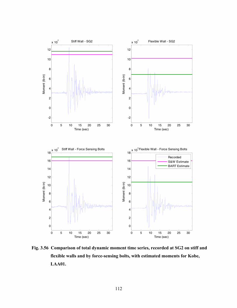
112
0 5 10 15 20 25 30
-2
0
2
4
6
8
10
12
x 107
Time (sec)
Mom
ent
(lb-in
)Stiff Wall - SG2
0 5 10 15 20 25 30
-2
0
2
4
6
8
10
12
x 107
Time (sec)
Mom
ent
(lb-in
)
Flexible Wall - SG2
0 5 10 15 20 25 30
0
2
4
6
8
10
12
14
16
18x 10
7
Time (sec)
Mom
ent
(lb-in
)
Stiff Wall - Force Sensing Bolts
0 5 10 15 20 25 30
0
2
4
6
8
10
12
14
16
18x 10
7
Time (sec)
Mom
ent
(lb-in
)
Flexible Wall - Force Sensing Bolts
RecordedS&W EstimateBART Estimate
Fig. 3.56 Comparison of total dynamic moment time series, recorded at SG2 on stiff and
flexible walls and by force-sensing bolts, with estimated moments for Kobe,
LAA01.
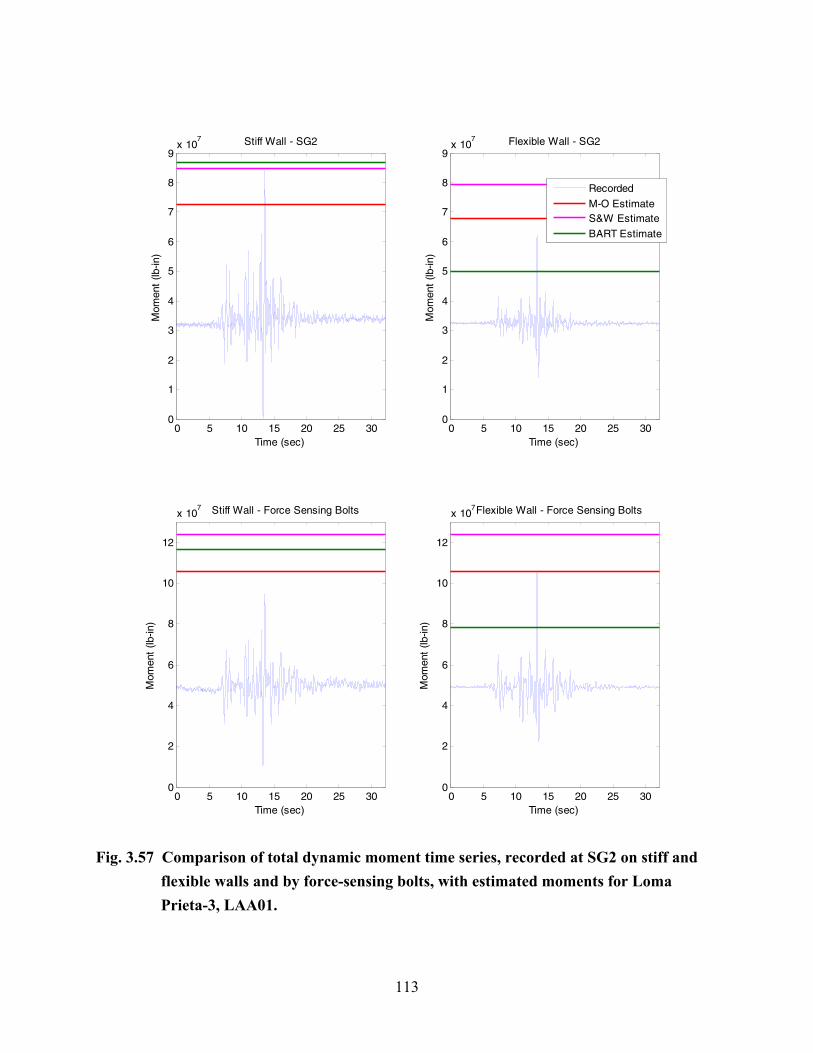
113
0 5 10 15 20 25 300
1
2
3
4
5
6
7
8
9x 10
7
Time (sec)
Mom
ent
(lb-in
)Stiff Wall - SG2
0 5 10 15 20 25 300
1
2
3
4
5
6
7
8
9x 10
7
Time (sec)M
omen
t (lb
-in)
Flexible Wall - SG2
0 5 10 15 20 25 300
2
4
6
8
10
12
x 107
Time (sec)
Mom
ent
(lb-in
)
Stiff Wall - Force Sensing Bolts
0 5 10 15 20 25 300
2
4
6
8
10
12
x 107
Time (sec)
Mom
ent
(lb-in
)
Flexible Wall - Force Sensing Bolts
RecordedM-O EstimateS&W EstimateBART Estimate
Fig. 3.57 Comparison of total dynamic moment time series, recorded at SG2 on stiff and flexible walls and by force-sensing bolts, with estimated moments for Loma Prieta-3, LAA01.

114
0 5 10 15 20 25 300
1
2
3
4
5
6
7
8x 10
7
Time (sec)
Mom
ent
(lb-in
)Stiff Wall - SG2
0 5 10 15 20 25 300
1
2
3
4
5
6
7
8x 10
7
Time (sec)
Mom
ent
(lb-in
)
Flexible Wall - SG2
0 5 10 15 20 25 30
0
2
4
6
8
10
12x 10
7
Time (sec)
Mom
ent
(lb-in
)
Stiff Wall - Force Sensing Bolts
0 5 10 15 20 25 30
0
2
4
6
8
10
12x 10
7
Time (sec)
Mom
ent
(lb-in
)
Flexible Wall - Force Sensing Bolts
RecordedM-O EstimateS&W EstimateBART Estimate
Fig. 3.58 Comparison of total dynamic moment time histories, recorded at SG2 on stiff and flexible walls and by force-sensing bolts, with estimated moments for Loma Prieta-SC-1, LAA02.

115
0 5 10 15 20 25 30
-2
0
2
4
6
8
10
12
x 107
Time (sec)
Mom
ent
(lb-in
)Stiff Wall - SG2
0 5 10 15 20 25 30
-2
0
2
4
6
8
10
12
x 107
Time (sec)
Mom
ent
(lb-in
)
Flexible Wall - SG2
0 5 10 15 20 25 30
-2
0
2
4
6
8
10
12
14
16
18x 10
7
Time (sec)
Mom
ent
(lb-in
)
Stiff Wall - Force Sensing Bolts
0 5 10 15 20 25 30
-2
0
2
4
6
8
10
12
14
16
18x 10
7
Time (sec)
Mom
ent
(lb-in
)
Flexible Wall - Force Sensing Bolts
RecordedM-O EstimateS&W EstimateBART Estimate
Fig. 3.59 Comparison of total dynamic moment time histories, recorded at SG2 on stiff and flexible walls and by force-sensing bolts, with estimated moments for Kobe-PI-1, LAA02.

116
0 5 10 15 20 25 30
-2
0
2
4
6
8
10
12
x 107
Time (sec)
Mom
ent
(lb-in
)Stiff Wall - SG2
0 5 10 15 20 25 30
-2
0
2
4
6
8
10
12
x 107
Time (sec)
Mom
ent
(lb-in
)
Flexible Wall - SG2
0 5 10 15 20 25 30
-2
0
2
4
6
8
10
12
14
16
18x 10
7
Time (sec)
Mom
ent
(lb-in
)
Stiff Wall - Force Sensing Bolts
0 5 10 15 20 25 30
-2
0
2
4
6
8
10
12
14
16
18x 10
7
Time (sec)
Mom
ent
(lb-in
)
Flexible Wall - Force Sensing Bolts
RecordedS&W EstimateBART Estimate
Fig. 3.60 Comparison of total dynamic moment time histories, recorded at SG2 on stiff and flexible walls and by force-sensing bolts, with estimated moments for Kobe-PI-2, LAA02.

117
0 5 10 15 20 25 30-1
0
1
2
3
4
5
6
7
8
9
10x 10
7
Time (sec)
Mom
ent
(lb-in
)Stiff Wall - SG2
0 5 10 15 20 25 30-1
0
1
2
3
4
5
6
7
8
9
10x 10
7
Time (sec)
Mom
ent
(lb-in
)
Flexible Wall - SG2
0 5 10 15 20 25 30-2
0
2
4
6
8
10
12
x 107
Time (sec)
Mom
ent
(lb-in
)
Stiff Wall - Force Sensing Bolts
0 5 10 15 20 25 30-2
0
2
4
6
8
10
12
x 107
Time (sec)
Mom
ent
(lb-in
)
Flexible Wall - Force Sensing Bolts
RecordedM-O EstimateS&W EstimateBART Estimate
Fig. 3.61 Comparison of total dynamic moment time histories, recorded at SG2 on stiff and flexible walls and by force-sensing bolts, with estimated moments for Loma Prieta-SC-2, LAA02.

118
0 5 10 15 20 25 301
1.5
2
2.5
3
3.5
4
4.5
5
5.5
6x 10
7
Time (sec)
Mom
ent
(lb-in
)Stiff Wall - SG2
0 5 10 15 20 25 301
1.5
2
2.5
3
3.5
4
4.5
5
5.5
6x 10
7
Time (sec)
Mom
ent
(lb-in
)
Flexible Wall - SG2
0 5 10 15 20 25 300
1
2
3
4
5
6
7
8
9
10x 10
7
Time (sec)
Mom
ent
(lb-in
)
Stiff Wall - Force Sensing Bolts
0 5 10 15 20 25 300
1
2
3
4
5
6
7
8
9
10x 10
7
Time (sec)
Mom
ent
(lb-in
)
Flexible Wall - Force Sensing Bolts
RecordedM-O EstimateS&W EstimateBART Estimate
Fig. 3.62 Comparison of total dynamic moment time histories, recorded at SG2 on stiff and flexible walls and by force-sensing bolts, with estimated moments for Kocaeli-YPT060-2, LAA02.
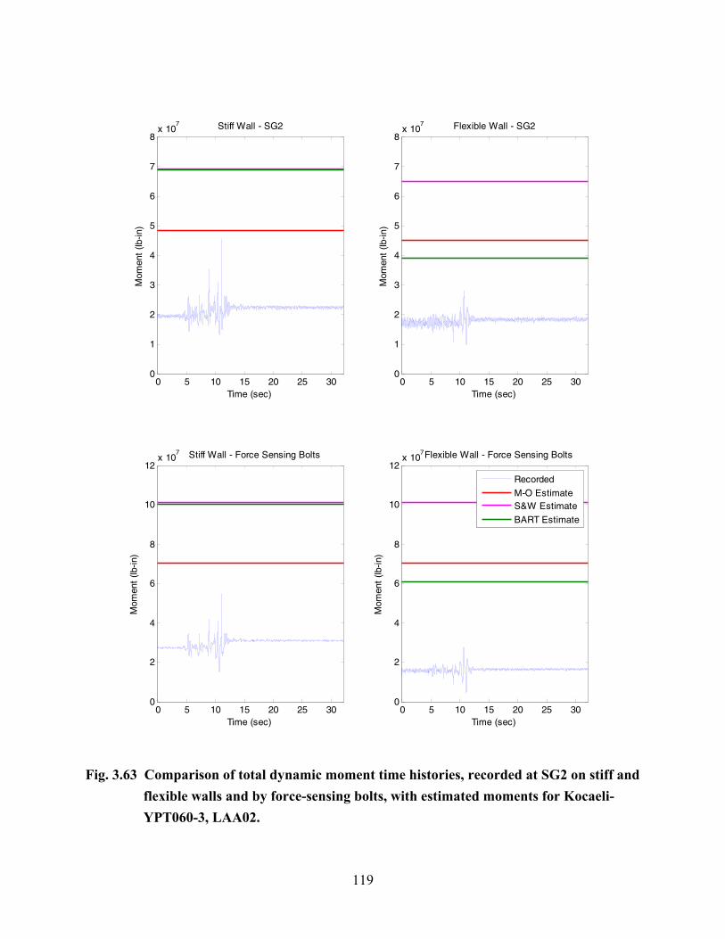
119
0 5 10 15 20 25 300
1
2
3
4
5
6
7
8x 10
7
Time (sec)
Mom
ent
(lb-in
)Stiff Wall - SG2
0 5 10 15 20 25 300
1
2
3
4
5
6
7
8x 10
7
Time (sec)M
omen
t (lb
-in)
Flexible Wall - SG2
0 5 10 15 20 25 300
2
4
6
8
10
12x 10
7
Time (sec)
Mom
ent
(lb-in
)
Stiff Wall - Force Sensing Bolts
0 5 10 15 20 25 300
2
4
6
8
10
12x 10
7
Time (sec)
Mom
ent
(lb-in
)
Flexible Wall - Force Sensing Bolts
RecordedM-O EstimateS&W EstimateBART Estimate
Fig. 3.63 Comparison of total dynamic moment time histories, recorded at SG2 on stiff and flexible walls and by force-sensing bolts, with estimated moments for Kocaeli-YPT060-3, LAA02.

120
0 5 10 15 20 25 300
1
2
3
4
5
6
7
8x 10
7
Time (sec)
Mom
ent
(lb-in
)Stiff Wall - SG2
0 5 10 15 20 25 300
1
2
3
4
5
6
7
8x 10
7
Time (sec)M
omen
t (lb
-in)
Flexible Wall - SG2
0 5 10 15 20 25 300
1
2
3
4
5
6
7
8
9
10
11x 10
7
Time (sec)
Mom
ent
(lb-in
)
Stiff Wall - Force Sensing Bolts
0 5 10 15 20 25 300
1
2
3
4
5
6
7
8
9
10
11x 10
7
Time (sec)
Mom
ent
(lb-in
)
Flexible Wall - Force Sensing Bolts
RecordedM-O EstimateS&W EstimateBART Estimate
Fig. 3.64 Comparison of total dynamic moment time histories, recorded at SG2 on stiff and flexible walls and by force-sensing bolts, with estimated moments for Kocaeli-YPT330-2, LAA02.
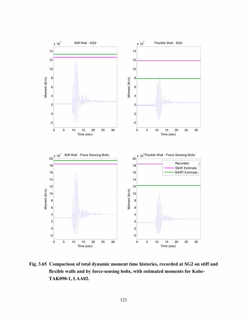
121
0 5 10 15 20 25 30
-2
0
2
4
6
8
10
12
14
x 107
Time (sec)
Mom
ent
(lb-in
)Stiff Wall - SG2
0 5 10 15 20 25 30
-2
0
2
4
6
8
10
12
14
x 107
Time (sec)
Mom
ent
(lb-in
)
Flexible Wall - SG2
0 5 10 15 20 25 30
-2
0
2
4
6
8
10
12
14
16
18
20x 10
7
Time (sec)
Mom
ent
(lb-in
)
Stiff Wall - Force Sensing Bolts
0 5 10 15 20 25 30
-2
0
2
4
6
8
10
12
14
16
18
20x 10
7
Time (sec)
Mom
ent
(lb-in
)
Flexible Wall - Force Sensing Bolts
RecordedS&W EstimateBART Estimate
Fig. 3.65 Comparison of total dynamic moment time histories, recorded at SG2 on stiff and flexible walls and by force-sensing bolts, with estimated moments for Kobe-TAK090-1, LAA02.

122
0 5 10 15 20 25 30-2
0
2
4
6
8
10
x 107
Time (sec)
Mom
ent
(lb-in
)Stiff Wall - SG2
0 5 10 15 20 25 30
0
2
4
6
8
10
x 107
Time (sec)
Mom
ent
(lb-in
)
Flexible Wall - SG2
0 5 10 15 20 25 30
0
5
10
15x 10
7
Time (sec)
Mom
ent
(lb-in
)
Stiff Wall - Force Sensing Bolts
0 5 10 15 20 25 30
0
5
10
15x 10
7
Time (sec)
Mom
ent
(lb-in
)
Flexible Wall - Force Sensing Bolts
RecordedM-O EstimateS&W EstimateBART Estimate
Fig. 3.66 Comparison of total dynamic moment time histories, recorded at SG2 on stiff and flexible walls and by force-sensing bolts, with estimated moments for Kobe-TAK090-2, LAA02.

123
0 5 10 15 20 25 301
1.5
2
2.5
3
3.5
4
4.5
5
5.5
6x 10
7
Time (sec)
Mom
ent
(lb-in
)Stiff Wall - SG2
0 5 10 15 20 25 301
1.5
2
2.5
3
3.5
4
4.5
5
5.5
6x 10
7
Time (sec)
Mom
ent
(lb-in
)
Flexible Wall - SG2
0 5 10 15 20 25 301
2
3
4
5
6
7
8
9x 10
7
Time (sec)
Mom
ent
(lb-in
)
Stiff Wall - Force Sensing Bolts
0 5 10 15 20 25 301
2
3
4
5
6
7
8
9x 10
7
Time (sec)
Mom
ent
(lb-in
)
Flexible Wall - Force Sensing Bolts
RecordedM-O EstimateS&W EstimateBART Estimate
Fig. 3.67 Comparison of total dynamic moment time histories, recorded at SG2 on stiff and flexible walls and by force-sensing bolts, with estimated moments for Loma Prieta-WVC270, LAA02.

124
0 5 10 15 20 25 301
2
3
4
5
6
7x 10
7
Time (sec)
Mom
ent
(lb-in
)Stiff Wall - SG2
0 5 10 15 20 25 301
2
3
4
5
6
7x 10
7
Time (sec)M
omen
t (lb
-in)
Flexible Wall - SG2
0 5 10 15 20 25 301
2
3
4
5
6
7
8
9
10x 10
7
Time (sec)
Mom
ent
(lb-in
)
Stiff Wall - Force Sensing Bolts
0 5 10 15 20 25 301
2
3
4
5
6
7
8
9
10x 10
7
Time (sec)
Mom
ent
(lb-in
)
Flexible Wall - Force Sensing Bolts
RecordedM-O EstimateS&W EstimateBART Estimate
Fig. 3.68 Comparison of total dynamic moment time histories, recorded at SG2 on stiff and flexible walls and by force-sensing bolts, with estimated moments for Kocaeli-YPT330-3, LAA02.

125
As shown in Figures 3.54–3.57 for experiment LAA01, the moments measured at the
base of the stiff wall are generally adequately estimated by the M-O method and the BART
design criteria and overestimated by the Seed and Whitman (1970) method. For the Kobe
shaking event, the Seed and Whitman (1970) method slightly underestimated the moments
measured on the stiff wall in one cycle. The peak moments measured on the flexible wall were
generally underestimated by the M-O method and the BART design criteria. We note that there
was period matching between the Loma Prieta shaking events in experiment LAA01 and the
flexible walls, hence the large observed moments.
As shown in Figures 3.58–3.68 for experiment LAA02, BART design criteria for stiff
and flexible retaining walls, as well as the Seed and Whitman method, generally overestimate the
dynamic moment distributions at all times for all shaking events except for some of the Kobe
shakes. During the early LAA02 motions, recorded dynamic moments slightly exceeded BART’s
estimated dynamic moments on the stiff and flexible walls. This phenomenon was not observed
during the later Kobe shaking events due to the densification of the soil.
In addition the time history data clearly show the effect of soil densification during the
shaking as the static moment on the walls increases during the shaking. This effect is most
pronounced for the strongest shaking events with largest amount of settlement. Such effect
would be less pronounced in soils that are less susceptible to compaction either due to greater
density or presence of cohesion. Finally, the time histories show that the total dynamic
moments, which include the moments due to the wall inertia, rarely exceed the design criteria in
more than one cycle.
3.8 PERFORMANCE: DYNAMIC MOMENT INCREMENT TIME HISTORIES
As already discussed in Section 3.4.5 and as noted above, the total dynamic moments incorporate
moments due to the static earth pressure, the static earth pressure increment due to compaction
during shaking and, of course, the moment due to the dynamic response of the wall itself. Thus,
the data were processed to eliminate the static moments and the static moment increment due to
shaking. The resulting plots are presented in Figures 3.69–3.83. In general, these results show a
pattern consistent with that observed for the maximum total moments, as would be expected.

126
0 5 10 15 20 25 30-4
-3
-2
-1
0
1
2
3
4
5
6x 10
7
Time (sec)
Dyn
amic
Mom
ent
Incr
emen
t(lb
-in)
Stiff Wall - SG2
0 5 10 15 20 25 30-4
-3
-2
-1
0
1
2
3
4
5
6x 10
7
Time (sec)D
ynam
ic M
omen
t In
crem
ent(
lb-in
)
Flexible Wall - SG2
0 5 10 15 20 25 30-5
0
5
10x 10
7
Time (sec)
Dyn
amic
Mom
ent
Incr
emen
t(lb
-in)
Stiff Wall - Force Sensing Bolts
0 5 10 15 20 25 30-5
0
5
10x 10
7
Time (sec)
Dyn
amic
Mom
ent
Incr
emen
t(lb
-in)
Flexible Wall - Force Sensing Bolts
RecordedM-O EstimateS&W EstimateBART Estimate
Fig. 3.69 Comparison of dynamic moment increment time series, recorded at SG2 on stiff and flexible walls and by force-sensing bolts, with estimated moments for Loma Prieta-1, LAA01.

127
0 5 10 15 20 25 30-4
-3
-2
-1
0
1
2
3
4
5
6x 10
7
Time (sec)
Dyn
amic
Mom
ent
Incr
emen
t(lb
-in)
Stiff Wall - SG2
0 5 10 15 20 25 30-4
-3
-2
-1
0
1
2
3
4
5
6x 10
7
Time (sec)D
ynam
ic M
omen
t In
crem
ent(
lb-in
)
Flexible Wall - SG2
0 5 10 15 20 25 30-5
0
5
10x 10
7
Time (sec)
Dyn
amic
Mom
ent
Incr
emen
t(lb
-in)
Stiff Wall - Force Sensing Bolts
0 5 10 15 20 25 30-5
0
5
10x 10
7
Time (sec)
Dyn
amic
Mom
ent
Incr
emen
t(lb
-in)
Flexible Wall - Force Sensing Bolts
RecordedM-O EstimateS&W EstimateBART Estimate
Fig. 3.70 Comparison of dynamic moment increment time series, recorded at SG2 on stiff and flexible walls and by force-sensing bolts, with estimated moments for Loma Prieta-2, LAA01.

128
0 5 10 15 20 25 30-5
0
5
10x 10
7
Time (sec)
Dyn
amic
Mom
ent
Incr
emen
t(lb
-in)
Stiff Wall - SG2
0 5 10 15 20 25 30-5
0
5
10x 10
7
Time (sec)
Dyn
amic
Mom
ent
Incr
emen
t(lb
-in)
Flexible Wall - SG2
0 5 10 15 20 25 30-6
-4
-2
0
2
4
6
8
10
12
14
x 107
Time (sec)
Dyn
amic
Mom
ent
Incr
emen
t(lb
-in)
Stiff Wall - Force Sensing Bolts
0 5 10 15 20 25 30-6
-4
-2
0
2
4
6
8
10
12
14
x 107
Time (sec)
Dyn
amic
Mom
ent
Incr
emen
t(lb
-in)
Flexible Wall - Force Sensing Bolts
RecordedS&W EstimateBART Estimate
Fig. 3.71 Comparison of dynamic moment increment time series, recorded at SG2 on stiff and flexible walls and by force-sensing bolts, with estimated moments for Kobe, LAA01.

129
0 5 10 15 20 25 30
-4
-2
0
2
4
6
8x 10
7
Time (sec)
Dyn
amic
Mom
ent
Incr
emen
t(lb
-in)
Stiff Wall - SG2
0 5 10 15 20 25 30
-4
-2
0
2
4
6
8x 10
7
Time (sec)D
ynam
ic M
omen
t In
crem
ent(
lb-in
)
Flexible Wall - SG2
0 5 10 15 20 25 30-5
0
5
10x 10
7
Time (sec)
Dyn
amic
Mom
ent
Incr
emen
t(lb
-in)
Stiff Wall - Force Sensing Bolts
0 5 10 15 20 25 30-5
0
5
10x 10
7
Time (sec)
Dyn
amic
Mom
ent
Incr
emen
t(lb
-in)
Flexible Wall - Force Sensing Bolts
RecordedM-O EstimateS&W EstimateBART Estimate
Fig. 3.72 Comparison of dynamic moment increment time series, recorded at SG2 on stiff and flexible walls and by force-sensing bolts, with estimated moments for Loma Prieta-3, LAA01.

130
0 5 10 15 20 25 30-3
-2
-1
0
1
2
3
4
5
6x 10
7
Time (sec)
Dyn
amic
Mom
ent
Incr
emen
t(lb
-in)
Stiff Wall - SG2
0 5 10 15 20 25 30-3
-2
-1
0
1
2
3
4
5
6x 10
7
Time (sec)D
ynam
ic M
omen
t In
crem
ent(
lb-in
)
Flexible Wall - SG2
0 5 10 15 20 25 30-3
-2
-1
0
1
2
3
4
5
6
7
8x 10
7
Time (sec)
Dyn
amic
Mom
ent
Incr
emen
t(lb
-in)
Stiff Wall - Force Sensing Bolts
0 5 10 15 20 25 30-3
-2
-1
0
1
2
3
4
5
6
7
8x 10
7
Time (sec)
Dyn
amic
Mom
ent
Incr
emen
t(lb
-in)
Flexible Wall - Force Sensing Bolts
RecordedM-O EstimateS&W EstimateBART Estimate
Fig. 3.73 Comparison of dynamic moment increment time series, recorded at SG2 on stiff and flexible walls and by force-sensing bolts, with estimated moments for Loma Prieta-SC-1, LAA02.

131
0 5 10 15 20 25 30-5
0
5
10x 10
7
Time (sec)
Dyn
amic
Mom
ent
Incr
emen
t(lb
-in)
Stiff Wall - SG2
0 5 10 15 20 25 30-5
0
5
10x 10
7
Time (sec)
Dyn
amic
Mom
ent
Incr
emen
t(lb
-in)
Flexible Wall - SG2
0 5 10 15 20 25 30-5
0
5
10
15x 10
7
Time (sec)
Dyn
amic
Mom
ent
Incr
emen
t(lb
-in)
Stiff Wall - Force Sensing Bolts
0 5 10 15 20 25 30-5
0
5
10
15x 10
7
Time (sec)
Dyn
amic
Mom
ent
Incr
emen
t(lb
-in)
Flexible Wall - Force Sensing Bolts
RecordedM-O EstimateS&W EstimateBART Estimate
Fig. 3.74 Comparison of dynamic moment increment time series, recorded at SG2 on stiff and flexible walls and by force-sensing bolts, with estimated moments for Kobe-PI-1, LAA02.
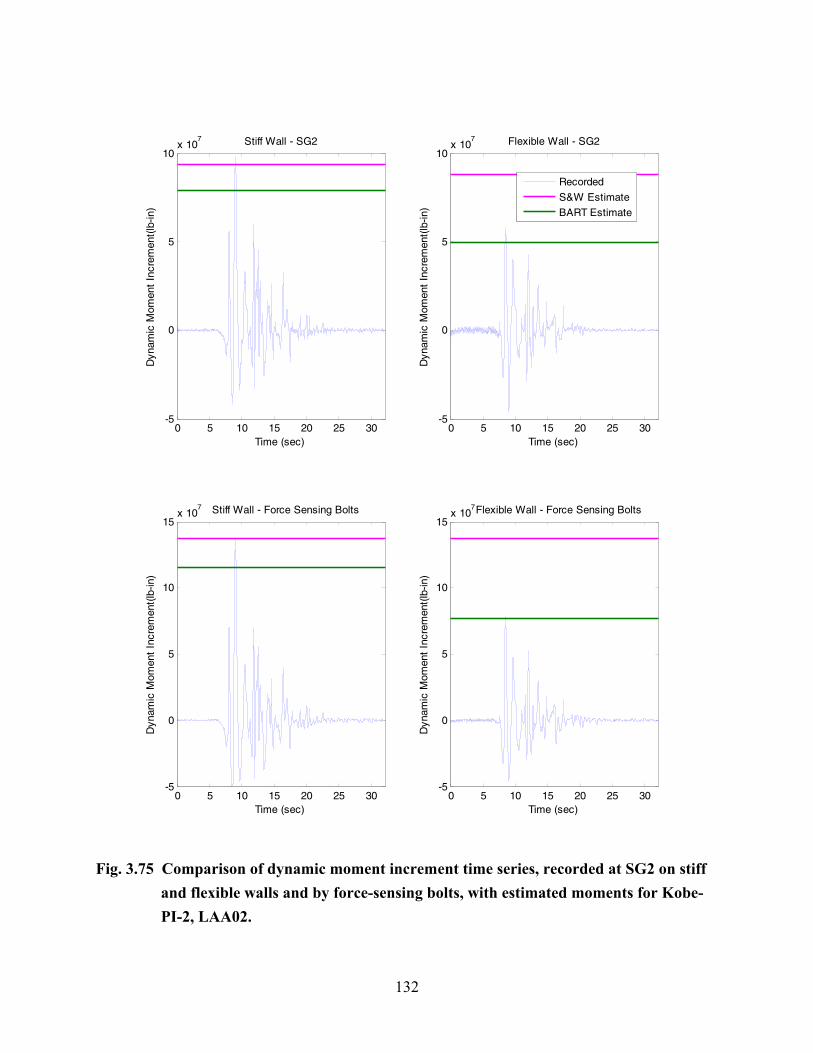
132
0 5 10 15 20 25 30-5
0
5
10x 10
7
Time (sec)
Dyn
amic
Mom
ent
Incr
emen
t(lb
-in)
Stiff Wall - SG2
0 5 10 15 20 25 30-5
0
5
10x 10
7
Time (sec)
Dyn
amic
Mom
ent
Incr
emen
t(lb
-in)
Flexible Wall - SG2
0 5 10 15 20 25 30-5
0
5
10
15x 10
7
Time (sec)
Dyn
amic
Mom
ent
Incr
emen
t(lb
-in)
Stiff Wall - Force Sensing Bolts
0 5 10 15 20 25 30-5
0
5
10
15x 10
7
Time (sec)
Dyn
amic
Mom
ent
Incr
emen
t(lb
-in)
Flexible Wall - Force Sensing Bolts
RecordedS&W EstimateBART Estimate
Fig. 3.75 Comparison of dynamic moment increment time series, recorded at SG2 on stiff and flexible walls and by force-sensing bolts, with estimated moments for Kobe-PI-2, LAA02.

133
0 5 10 15 20 25 30-3
-2
-1
0
1
2
3
4
5
6
7
8x 10
7
Time (sec)
Dyn
amic
Mom
ent
Incr
emen
t(lb
-in)
Stiff Wall - SG2
0 5 10 15 20 25 30-3
-2
-1
0
1
2
3
4
5
6
7
8x 10
7
Time (sec)D
ynam
ic M
omen
t In
crem
ent(
lb-in
)
Flexible Wall - SG2
0 5 10 15 20 25 30-5
0
5
10x 10
7
Time (sec)
Dyn
amic
Mom
ent
Incr
emen
t(lb
-in)
Stiff Wall - Force Sensing Bolts
0 5 10 15 20 25 30-5
0
5
10x 10
7
Time (sec)
Dyn
amic
Mom
ent
Incr
emen
t(lb
-in)
Flexible Wall - Force Sensing Bolts
RecordedM-O EstimateS&W EstimateBART Estimate
Fig. 3.76 Comparison of dynamic moment increment time series, recorded at SG2 on stiff and flexible walls and by force-sensing bolts, with estimated moments for Loma Prieta-SC-2, LAA02.
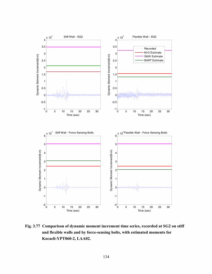
134
0 5 10 15 20 25 30-1
-0.5
0
0.5
1
1.5
2
2.5
3
3.5
4x 10
7
Time (sec)
Dyn
amic
Mom
ent
Incr
emen
t(lb
-in)
Stiff Wall - SG2
0 5 10 15 20 25 30-1
-0.5
0
0.5
1
1.5
2
2.5
3
3.5
4x 10
7
Time (sec)
Dyn
amic
Mom
ent
Incr
emen
t(lb
-in)
Flexible Wall - SG2
0 5 10 15 20 25 30-2
-1
0
1
2
3
4
5
6x 10
7
Time (sec)
Dyn
amic
Mom
ent
Incr
emen
t(lb
-in)
Stiff Wall - Force Sensing Bolts
0 5 10 15 20 25 30-2
-1
0
1
2
3
4
5
6x 10
7
Time (sec)
Dyn
amic
Mom
ent
Incr
emen
t(lb
-in)
Flexible Wall - Force Sensing Bolts
RecordedM-O EstimateS&W EstimateBART Estimate
Fig. 3.77 Comparison of dynamic moment increment time series, recorded at SG2 on stiff and flexible walls and by force-sensing bolts, with estimated moments for Kocaeli-YPT060-2, LAA02.

135
0 5 10 15 20 25 30-2
-1
0
1
2
3
4
5
6x 10
7
Time (sec)
Dyn
amic
Mom
ent
Incr
emen
t(lb
-in)
Stiff Wall - SG2
0 5 10 15 20 25 30-2
-1
0
1
2
3
4
5
6x 10
7
Time (sec)D
ynam
ic M
omen
t In
crem
ent(
lb-in
)
Flexible Wall - SG2
0 5 10 15 20 25 30-2
-1
0
1
2
3
4
5
6
7
8x 10
7
Time (sec)
Dyn
amic
Mom
ent
Incr
emen
t(lb
-in)
Stiff Wall - Force Sensing Bolts
0 5 10 15 20 25 30-2
-1
0
1
2
3
4
5
6
7
8x 10
7
Time (sec)
Dyn
amic
Mom
ent
Incr
emen
t(lb
-in)
Flexible Wall - Force Sensing Bolts
RecordedM-O EstimateS&W EstimateBART Estimate
Fig. 3.78 Comparison of dynamic moment increment time series, recorded at SG2 on stiff and flexible walls and by force-sensing bolts, with estimated moments for Kocaeli-YPT060-3, LAA02.

136
0 5 10 15 20 25 30-2
-1
0
1
2
3
4
5
6x 10
7
Time (sec)
Dyn
amic
Mom
ent
Incr
emen
t(lb
-in)
Stiff Wall - SG2
0 5 10 15 20 25 30-2
-1
0
1
2
3
4
5
6x 10
7
Time (sec)D
ynam
ic M
omen
t In
crem
ent(
lb-in
)
Flexible Wall - SG2
0 5 10 15 20 25 30-2
-1
0
1
2
3
4
5
6
7
8x 10
7
Time (sec)
Dyn
amic
Mom
ent
Incr
emen
t(lb
-in)
Stiff Wall - Force Sensing Bolts
0 5 10 15 20 25 30-2
-1
0
1
2
3
4
5
6
7
8x 10
7
Time (sec)
Dyn
amic
Mom
ent
Incr
emen
t(lb
-in)
Flexible Wall - Force Sensing Bolts
RecordedM-O EstimateS&W EstimateBART Estimate
Fig. 3.79 Comparison of dynamic moment increment time series, recorded at SG2 on stiff and flexible walls and by force-sensing bolts, with estimated moments for Kocaeli-YPT330-2, LAA02.

137
0 5 10 15 20 25 30
-4
-2
0
2
4
6
8
10
12x 10
7
Time (sec)
Dyn
amic
Mom
ent
Incr
emen
t(lb
-in)
Stiff Wall - SG2
0 5 10 15 20 25 30
-4
-2
0
2
4
6
8
10
12x 10
7
Time (sec)
Dyn
amic
Mom
ent
Incr
emen
t(lb
-in)
Flexible Wall - SG2
0 5 10 15 20 25 30-1
-0.5
0
0.5
1
1.5
x 108
Time (sec)
Dyn
amic
Mom
ent
Incr
emen
t(lb
-in)
Stiff Wall - Force Sensing Bolts
0 5 10 15 20 25 30-1
-0.5
0
0.5
1
1.5
x 108
Time (sec)
Dyn
amic
Mom
ent
Incr
emen
t(lb
-in)
Flexible Wall - Force Sensing Bolts
RecordedS&W EstimateBART Estimate
Fig. 3.80 Comparison of dynamic moment increment time series, recorded at SG2 on stiff and flexible walls and by force-sensing bolts, with estimated moments for Kobe-TAK090-1, LAA02.
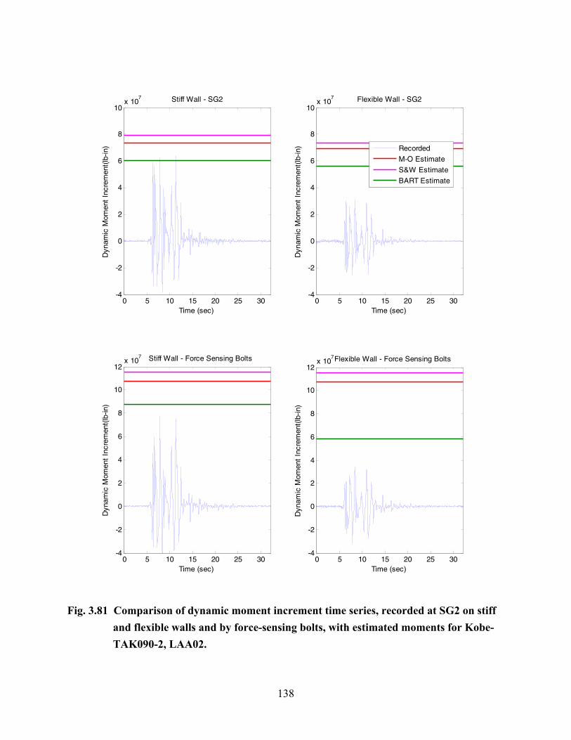
138
0 5 10 15 20 25 30-4
-2
0
2
4
6
8
10x 10
7
Time (sec)
Dyn
amic
Mom
ent
Incr
emen
t(lb
-in)
Stiff Wall - SG2
0 5 10 15 20 25 30-4
-2
0
2
4
6
8
10x 10
7
Time (sec)
Dyn
amic
Mom
ent
Incr
emen
t(lb
-in)
Flexible Wall - SG2
0 5 10 15 20 25 30-4
-2
0
2
4
6
8
10
12x 10
7
Time (sec)
Dyn
amic
Mom
ent
Incr
emen
t(lb
-in)
Stiff Wall - Force Sensing Bolts
0 5 10 15 20 25 30-4
-2
0
2
4
6
8
10
12x 10
7
Time (sec)
Dyn
amic
Mom
ent
Incr
emen
t(lb
-in)
Flexible Wall - Force Sensing Bolts
RecordedM-O EstimateS&W EstimateBART Estimate
Fig. 3.81 Comparison of dynamic moment increment time series, recorded at SG2 on stiff and flexible walls and by force-sensing bolts, with estimated moments for Kobe-TAK090-2, LAA02.

139
0 5 10 15 20 25 30-1
-0.5
0
0.5
1
1.5
2
2.5
3
3.5
4x 10
7
Time (sec)
Dyn
amic
Mom
ent
Incr
emen
t(lb
-in)
Stiff Wall - SG2
0 5 10 15 20 25 30-1
-0.5
0
0.5
1
1.5
2
2.5
3
3.5
4x 10
7
Time (sec)
Dyn
amic
Mom
ent
Incr
emen
t(lb
-in)
Flexible Wall - SG2
0 5 10 15 20 25 30-2
-1
0
1
2
3
4
5
6x 10
7
Time (sec)
Dyn
amic
Mom
ent
Incr
emen
t(lb
-in)
Stiff Wall - Force Sensing Bolts
0 5 10 15 20 25 30-2
-1
0
1
2
3
4
5
6x 10
7
Time (sec)
Dyn
amic
Mom
ent
Incr
emen
t(lb
-in)
Flexible Wall - Force Sensing Bolts
RecordedM-O EstimateS&W EstimateBART Estimate
Fig. 3.82 Comparison of dynamic moment increment time series, recorded at SG2 on stiff and flexible walls and by force-sensing bolts, with estimated moments for Loma Prieta-WVC270, LAA02.

140
0 5 10 15 20 25 30-1
0
1
2
3
4
5
6x 10
7
Time (sec)
Dyn
amic
Mom
ent
Incr
emen
t(lb
-in)
Stiff Wall - SG2
0 5 10 15 20 25 30-1
0
1
2
3
4
5
6x 10
7
Time (sec)D
ynam
ic M
omen
t In
crem
ent(
lb-in
)
Flexible Wall - SG2
0 5 10 15 20 25 30-2
-1
0
1
2
3
4
5
6
7
8x 10
7
Time (sec)
Dyn
amic
Mom
ent
Incr
emen
t(lb
-in)
Stiff Wall - Force Sensing Bolts
0 5 10 15 20 25 30-2
-1
0
1
2
3
4
5
6
7
8x 10
7
Time (sec)
Dyn
amic
Mom
ent
Incr
emen
t(lb
-in)
Flexible Wall - Force Sensing Bolts
RecordedM-O EstimateS&W EstimateBART Estimate
Fig. 3.83 Comparison of dynamic moment increment time series, recorded at SG2 on stiff and flexible walls and by force-sensing bolts, with estimated moments for Kocaeli-YPT330-3, LAA02.
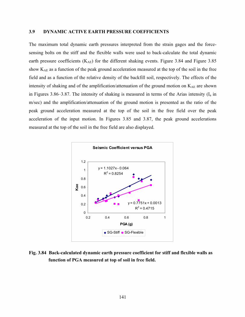
141
3.9 DYNAMIC ACTIVE EARTH PRESSURE COEFFICIENTS
The maximum total dynamic earth pressures interpreted from the strain gages and the force-
sensing bolts on the stiff and the flexible walls were used to back-calculate the total dynamic
earth pressure coefficients (KAE) for the different shaking events. Figure 3.84 and Figure 3.85
show KAE as a function of the peak ground acceleration measured at the top of the soil in the free
field and as a function of the relative density of the backfill soil, respectively. The effects of the
intensity of shaking and of the amplification/attenuation of the ground motion on KAE are shown
in Figures 3.86–3.87. The intensity of shaking is measured in terms of the Arias intensity (Ia in
m/sec) and the amplification/attenuation of the ground motion is presented as the ratio of the
peak ground acceleration measured at the top of the soil in the free field over the peak
acceleration of the input motion. In Figures 3.85 and 3.87, the peak ground accelerations
measured at the top of the soil in the free field are also displayed.
Seismic Coefficient versus PGA
y = 1.1027x - 0.064R2 = 0.8254
y = 0.7751x + 0.0013R2 = 0.4715
0
0.2
0.4
0.6
0.8
1
1.2
0.2 0.4 0.6 0.8 1
PGA (g)
Kae
SG-Stiff SG-Flexible
Fig. 3.84 Back-calculated dynamic earth pressure coefficient for stiff and flexible walls as function of PGA measured at top of soil in free field.

142
Seismic Coefficient versus Dr
0.36g0.52g
0.64g
0.4g
0.39g
0.76g 0.86g
0.3g
0.48g0.52g 0.44g
0.67g0.73g
0
0.2
0.4
0.6
0.8
1
1.2
60 65 70 75 80 85
Dr (%)
Kae
SG-Stiff
Seismic Coefficient versus Dr
0.3g0.4g0.39g0.28g
0.36g
0.52g
0.67g
0.76g
0.86g0.64g
0.52g0.44g
0.73g
0.48g0
0.2
0.4
0.6
0.8
1
1.2
60 65 70 75 80 85
Dr (%)
Kae
SG-Flexible
Fig. 3.85 Back-calculated dynamic earth pressure coefficient for stiff and flexible walls as function of relative density of soil backfill.
Seismic Coefficient versus amax,FF/amax,input
y = -0.3837x + 0.9645R2 = 0.4161
y = -0.2821x + 0.7388R2 = 0.2602
0
0.2
0.4
0.6
0.8
1
1.2
0.5 1 1.5 2
amax,FF/amax,input
Kae
SG-Stiff SG-Flexible
Fig. 3.86 Back-calculated dynamic earth pressure coefficient for stiff and flexible walls as function of amplification/attenuation of ground motion.

143
Seismic Coefficient versus Ia
0.64g
0.76g
0.67g
0.86g
0.44g0.52g
0.39g
0.28g0.3g
0.4g
0.73g
0.52g
0
0.2
0.4
0.6
0.8
1
1.2
0.1 1 10
Ia (m/sec)
Kae
SG-Stiff
Seismic Coefficient versus Ia
0.4g
0.31g
0.39g
0.36g0.48g
0.52g
0.52g
0.44g
0.28g
0.73
0.64g
0.86g 0.76g
0.67g
0
0.2
0.4
0.6
0.8
1
1.2
0.1 1 10
Ia (m/sec)
Kae
SG-Flexible Linear (SG-Flexible)
Fig. 3.87 Back-calculated dynamic earth pressure coefficient for stiff and flexible walls as function of intensity of shaking.
Figure 3.84 shows that the back-calculated dynamic earth pressure coefficient (KAE)
increases with increasing the peak ground acceleration measured at the top of the soil in the free
field. The effect of changing relative density on KAE is somewhat indistinct. While it appears
that there is a decrease in KAE with increasing relative density from 62 to 81%, this trend is not
very clear and is probably masked by the fact that the different ground motions were used at
different stages of the experiment. Another way to look at the results is to plot KAE as a function
of the amplification of the input ground motion in the free field. The plots in Fig 3.86 show that
the seismic earth pressure coefficient is the highest when the ground motion is attenuated
(stronger shaking) and decreases as the magnitude of ground motion amplification increases.
This effect is more clearly evident in Figure 3.87, which shows that the total seismic earth
pressure coefficient increases with the intensity of shaking represented by Ia.
The maximum dynamic increments of earth pressures interpreted from the strain gages and the
force-sensing bolts in both sets of experiments were used to back-calculate the dynamic earth
pressure increment coefficients (!KAE). Figure 3.88 and Figure 3.89 show !KAE as a function of
the peak ground acceleration measured at the top of the soil in the free field and as a function of
the relative density of the backfill soil, respectively. Figures 3.90–3.91 show !KAE as a function
of the intensity of shaking and of the amplification/attenuation of the ground motion,
respectively.

144
Seismic Coefficient Increment versus PGA
y = 1.1973x - 0.3293R2 = 0.8227
y = 0.635x - 0.171R2 = 0.735
0
0.2
0.4
0.6
0.8
0.2 0.4 0.6 0.8 1
PGA
!ka
e
SG-Stiff SG-Flexible
Fig. 3.88 Back-calculated dynamic earth pressure increment coefficient for stiff and flexible walls as function of PGA measured at top of soil in free field.
Seismic Coefficient Increment versus Dr
0.31g
0.4g
0.28g
0.36g0.39g
0.64g0.52g
0.86g
0.76g0.67g
0.44g0.52g
0.48g
0
0.2
0.4
0.6
0.8
60 64 68 72 76 80
Dr (%)
!ka
e
SG-Stiff
Seismic Coefficient Increment versus Dr
0.4g 0.36g0.28g
0.39g0.52g
0.73g0.48g
0.44g 0.64g
0.67g
0.52g
0.76g
0.86g
0
0.2
0.4
0.6
0.8
60 64 68 72 76 80
Dr (%)
!ka
e
SG-Flexible
Fig. 3.89 Back-calculated dynamic earth pressure increment coefficient for stiff and flexible walls as function of relative density of soil backfill.

145
Seismic Coefficient Increment versus amax, FF/amax, input
y = -0.4299x + 0.8031R2 = 0.4417
y = -0.1836x + 0.3774R2 = 0.2558
0
0.2
0.4
0.6
0.8
0.5 1 1.5 2
amax, FF/amax, input
!ka
e
SG-Stiff SG-Flexible
Fig. 3.90 Back-calculated dynamic earth pressure increment coefficient for stiff and flexible walls as function of amplification/attenuation of ground motion.
Seismic Coefficient Increment versus Ia
1.33
0.28
0.52g
0.28g0.39g0.4g 0.44g
0.86g0.67g0.76g
0.64g
0
0.2
0.4
0.6
0.8
0.1 1 10
Ia (m/sec)
!ka
e
SG-Stiff
Seismic Coefficient Increment versus Ia
0.48g
0.52g
0.28 0.36g0.39g
0.4g 0.64g0.73g
0.67g0.86g
0.76g
0.44g0.28g
0.52g
0
0.2
0.4
0.6
0.8
0.1 1 10
Ia (m/sec)
!ka
e
SG-Flexible
Fig. 3.91 Back-calculated dynamic earth pressure increment coefficient for stiff and flexible walls as function of intensity of shaking.
146
While these trends are consistent with those observed for the total dynamic earth pressure
coefficient, as would be expected, there is one very important observation that stands out. As
seen in Figure 3.88, dynamic effects do not appear to be significant when the PGA does not
exceed about 0.3 g. Similar effect can be seen in the relationship to the Arias intensity, with the
dynamic earth pressure coefficient remaining relatively small up to about 1 m/sec, which in our
case includes earthquake records with PGA in excess of 0.4 g.
3.10 WALL INERTIAL EFFECTS ON MOMENT AND PRESSURE DISTRIBUTIONS
During centrifuge experiment LAA02, the south stiff and the north flexible walls were
instrumented with accelerometers at the bases and the tops of the walls. The acceleration time
series recorded at these locations were used to determine the relative acceleration of the tops of
the stiff and flexible walls with respect to their bases and to estimate the moments induced at the
bases of the walls due to inertial effects. In this section, we assume that the acceleration on the
stiff and the flexible walls increases linearly from zero at the bases of the walls to a maximum at
the tops. The moments induced at the bases of the stiff and the flexible walls due to inertial
effects are estimated using relative acceleration values at the time the maximum total moment
profiles interpreted from the strain gages occurred.
Tables 3.33 and 3.34 show the relative accelerations and base moments applied on the
stiff and the flexible walls due to inertial effects for all shaking events during experiment
LAA02, respectively. Tables 3.33 and 3.34 also present the ratios of the moments induced at the
bases of the walls due to inertial effects to the maximum total dynamic moments at the bases
interpreted from the strain gage measurements.

147
Table 3.33 Estimate of moments induced at base of south stiff wall due to inertial effects for all shaking events during LAA02.
!a (g) M (lb-in) % of Maximum total Dynamic
Moment at the Base Loma Prieta-SC-1 0.78 1.96E+07 25.20% Kobe-PI-1 NA NA NA Kobe-PI-2 0.45 1.13E+07 7.65% Loma Prieta-SC-2 0.92 2.30E+07 26.39% Kocaeli-YPT060-2 0.33 8.24E+06 19.28% Kocaeli-YPT060-3 0.53 1.34E+07 20.74% Kocaeli-YPT330-2 0.44 1.10E+07 19.73% Kobe-TAK090-1 1.22 3.06E+07 19.02% Kobe-TAK090-2 0.87 2.19E+07 17.91% Loma Prieta-WVC270 0.21 5.34E+06 10.96% Kocaeli-YPT3303-3 0.36 9.05E+06 17.00%
Table 3.34 Estimate of moments induced at base of north flexible wall due to inertial effects for all shaking events during LAA02.
!a (g) M (lb-in) % of Maximum total Dynamic Moment at the Base
Loma Prieta-SC-1 0.44 8.90E+06 13.52% Kobe-PI-1 0.061 1.24E+06 1.07% Kobe-PI-2 0.634 1.28E+07 11.08% Loma Prieta-SC-2 0.32 6.41E+06 8.55% Kocaeli-YPT060-2 0.23 4.73E+06 13.50% Kocaeli-YPT060-3 0.09 1.81E+06 4.50% Kocaeli-YPT330-2 0.28 5.58E+06 13.29% Kobe-TAK090-1 NA NA NA Kobe-TAK090-2 0.97 1.96E+07 24.21% Loma Prieta-WVC270 0.38 7.78E+06 16.72% Kocaeli-YPT3303-3 0.21 4.24E+06 8.92%
Based on the results presented in Tables 3.33 and 3.34, the moments at the base of the
stiff wall due to wall inertial range, in general, from about 5–26% of the maximum total dynamic
moments interpreted from the strain gage data. The one outlier appears to be the Kobe-PI-1
earthquake in which the moment due to the inertia of the flexible wall to the maximum total
moment at the base was only 1%. At this point, further work is needed to fully interpret these

148
results in terms of their relationship to site period, Arias intensity, and period of the input
motion. Nevertheless, it is apparent that the total dynamic moments measured in the experiments
should be reduced by the appropriate factors to reflect moments induced by the earth pressure
alone.
Moreover the data show that inertial effects due to the mass of the walls are an important
element that has to be considered in the analysis and design. This aspect of the behavior of
gravity retaining structures was noted by Richards and Elms (1979) who concluded that the
effect of the wall inertia could be on the same order as that of the soil dynamic pressure
computed by the M-O analysis. Thus they strongly recommended that wall inertial effects
should be taken into account in the design of gravity retaining walls (Richards and Elms 1980) in
addition to the earth pressures obtained using the M-O analysis approach.
A somewhat different conclusion was reached by Clough and Fragaszy (1977) and
Fragaszy and Clough (1980) who investigated the seismic performance of cantilever retaining
structures. They analyzed the behavior of open channel floodway structures in the Greater Los
Angeles area during the 1971 San Fernando Valley earthquake. The floodway structures studied
consisted of open U-shaped channels with the walls tops set flush to the ground surface as shown
in Figure 3.92. The backfill soil consisted of dry medium-dense sand with an estimated friction
angle of 35°. The structures were designed for a conventional Rankine static triangular earth
pressure distribution, and no seismic provisions were applied in the design.
Fig. 3.92 Section through open channel floodway and typical mode of failure due to earthquake shaking (from Clough and Fragaszy 1977).
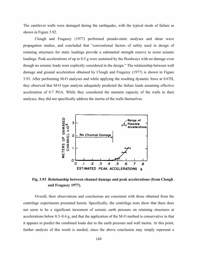
149
The cantilever walls were damaged during the earthquake, with the typical mode of failure as
shown in Figure 3.92.
Clough and Fragaszy (1977) performed pseudo-static analyses and shear wave
propagation studies, and concluded that “conventional factors of safety used in design of
retaining structures for static loadings provide a substantial strength reserve to resist seismic
loadings. Peak accelerations of up to 0.5 g were sustained by the floodways with no damage even
though no seismic loads were explicitly considered in the design.” The relationship between wall
damage and ground acceleration obtained by Clough and Fragazsy (1977) is shown in Figure
3.93. After performing M-O analyses and while applying the resulting dynamic force at 0.67H,
they observed that M-O type analysis adequately predicted the failure loads assuming effective
acceleration of 0.7 PGA. While they considered the moment capacity of the walls in their
analyses, they did not specifically address the inertia of the walls themselves.
Fig. 3.93 Relationship between channel damage and peak accelerations (from Clough and Fragaszy 1977).
Overall, their observations and conclusions are consistent with those obtained from the
centrifuge experiments presented herein. Specifically, the centrifuge tests show that there does
not seem to be a significant increment of seismic earth pressure on retaining structures at
accelerations below 0.3–0.4 g, and that the application of the M-O method is conservative in that
it appears to predict the combined loads due to the earth pressure and wall inertia. At this point,
further analysis of this result is needed, since the above conclusion may simply represent a

150
fortuitous outcome due to the assumption about the point of application of the seismic earth
pressure which is inconsistent with the conventional triangular distribution observed in our
experiments.
3.11 WALL DEFLECTIONS
Horizontal displacement transducers located at the tops of the stiff and flexible walls in both
experiments were used to measure the deflection at the tops of the walls during shaking as well
as the static offsets. Moreover, acceleration time series recorded at the tops of the walls were
double-integrated to obtain displacement time series that were compared to the time series
recorded by the displacement transducers. Static offsets cannot be obtained from the double
integration of the acceleration time series due to the high-pass filtering of the records. Also note
that the instrument rack to which the displacement transducers were attached experienced
vibration during spinning and shaking; this vibration is obvious in the recorded displacement
time series.
Table 3.35 presents the normalized static offsets measured at the tops of the four walls
after the different shaking events in both sets of experiments. The static offsets were normalized
by the heights of the walls. We note that the displacement time series for Kobe-PI-1, LAA02
were very noisy due to the power supply problem and therefore, the static offsets could not be
determined for this shaking event. Moreover, the two displacement transducers located at the top
of the north flexible (internal) wall were damaged in experiment LAA02 and are not available.
Tables 3.36 and 3.37 contain the maximum transient deflections during loading
normalized by the heights of the walls (H = 18.6 ft). The data show that the maximum
deflections measured at the tops of the walls by the displacement transducers did not always
agree well with the maximum deflections obtained by double-integrating the acceleration time
series. The rack vibration resulted in large apparent deflections and therefore, the maximum
deflections based on the acceleration time series are considered more accurate. Table 3.36 shows
that the maximum normalized transient deflections at the tops of the stiff walls exceeded 0.004H
for the LAA01 shaking events and for the Kobe motions during LAA02. Table 3.37 show that
the maximum normalized transient deflections at the tops of the flexible walls generally
exceeded 0.004H.

151
Table 3.35 Normalized static offsets increments measured at tops of walls after different shaking events.
Normalized Static Offsets at the Tops of the Walls Stiff Internal Stiff External Flexible Internal Flexible External Loma Prieta-1, LAA01 0.003 0.001 0.006 0.000 Loma Prieta-2, LAA01 0.001 0.000 0.001 0.001 Kobe, LAA01 0.001 0.001 0.001 0.001 Loma Prieta-3, LAA01 0.000 0.000 0.000 0.001 Loma Prieta-SC-1, LAA02 0.003 0.000 - 0.000
Kobe-PI-1, LAA02 - - - - Kobe-PI-2, LAA02 0.002 0.003 - 0.029 Loma Prieta-SC-2, LAA02 0.000 0.000 - 0.000
Kocaeli-YPT060-2, LAA02 0.000 0.001 - 0.001
Kocaeli-YPT060-3, LAA02 0.000 0.000 - 0.000
Kocaeli-YPT330-2, LAA02 0.000 0.000 - 0.002
Kobe-TAK090-1, LAA02 0.001 0.000 - 0.001
Kobe-TAK090-2, LAA02 0.000 0.000 - 0.000
Loma Prieta-WVC270, LAA02 0.000 0.000 - 0.000
Kocaeli-YPT330-3, LAA02 0.000 0.000 - 0.000
During experiment LAA02, the south stiff and north flexible walls were instrumented
with accelerometers located at the bases and the tops of the walls. The relative acceleration time
series of the tops of the walls with respect to their bases were double-integrated in order to obtain
the relative displacement of the tops of the south stiff and north flexible walls with respect to
their bases. Please note that the displacement of the tops of the walls with respect to their bases
could not be obtained in experiment LAA01 and for the north stiff and south flexible walls in
experiment LAA02 due to the absence of accelerometers at the bases. Table 3.38 presents the
maximum deflections at the tops of the south stiff and north flexible walls with respect to their
bases.

152
Table 3.36 Maximum transient deflections at tops of stiff walls during different shaking events.
Normalized Transient Deflections Stiff Internal Stiff External Disp. Transducers Acc. Records Disp. Transducers Acc. Records Loma Prieta-1, LAA01 0.008 0.008 0.009 0.020 Loma Prieta-2, LAA01 0.007 0.008 0.009 0.019 Kobe, LAA01 0.009 0.010 0.007 0.015 Loma Prieta-3, LAA01 0.007 0.010 0.010 0.020 Loma Prieta-SC-1, LAA02 0.001 0.004 0.001 0.002 Kobe-PI-1, LAA02 - 0.005 - 0.005 Kobe-PI-2, LAA02 0.014 0.004 0.019 0.004 Loma Prieta-SC-2, LAA02 0.009 0.002 0.016 0.002 Kocaeli-YPT060-2, LAA02 0.005 0.002 0.004 0.001 Kocaeli-YPT060-3, LAA02 0.007 0.002 0.006 0.001 Kocaeli-YPT330-2, LAA02 0.005 0.003 0.005 0.003 Kobe-TAK090-1, LAA02 0.021 0.008 0.032 0.004 Kobe-TAK090-2, LAA02 0.006 0.020 0.012 0.021 Loma Prieta-WVC270, LAA02 0.004 0.002 0.004 0.001 Kocaeli-YPT330-3, LAA02 0.005 0.002 0.006 0.001
Table 3.37 Maximum transient deflections at tops of flexible walls during different shaking events.
Normalized Transient Deflections Flexible Internal Flexible External Disp. Transducers Acc. Records Disp. Transducers Acc. Records Loma Prieta-1, LAA01 0.015 0.010 0.011 0.005 Loma Prieta-2, LAA01 0.013 0.010 0.011 0.007 Kobe, LAA01 0.011 0.012 0.013 0.017 Loma Prieta-3, LAA01 0.016 0.015 0.011 0.005 Loma Prieta-SC-1, LAA02 - 0.004 0.001 0.002 Kobe-PI-1, LAA02 - 0.018 - 0.003 Kobe-PI-2, LAA02 - 0.009 0.065 0.006 Loma Prieta-SC-2, LAA02 - 0.004 0.024 0.004 Kocaeli-YPT060-2, LAA02 - 0.002 0.005 - Kocaeli-YPT060-3, LAA02 - 0.003 0.009 - Kocaeli-YPT330-2, LAA02 - 0.004 0.005 0.003 Kobe-TAK090-1, LAA02 - 0.024 0.085 0.007 Kobe-TAK090-2, LAA02 - 0.019 0.028 0.024 Loma Prieta-WVC270, LAA02 - 0.003 0.004 0.001 Kocaeli-YPT330-3, LAA02 - 0.003 0.007 0.001

153
Table 3.38 Maximum deflections at tops of south stiff and north flexible walls with respect to their bases during different shaking events in experiment LAA02.
Normalized Relative Deflections Stiff Flexible Loma Prieta-SC-1 0.011 0.006 Kobe-PI-1 - 0.042 Kobe-PI-2 0.011 0.014 Loma Prieta-SC-2 0.005 0.007 Kocaeli-YPT060-2 0.001 0.002 Kocaeli-YPT060-3 0.002 0.003 Kocaeli-YPT330-2 0.002 0.003 Kobe-TAK090-1 0.010 0.613 Kobe-TAK090-2 0.007 0.007 Loma Prieta-WVC270 0.001 0.003 Kocaeli-YPT330-3 0.002 0.003
Overall, the data show that the walls showed very small, if any, permanent static
deflections. Under dynamic loading the flexible walls consistently exceeded the .004H deflection
limit, while the stiff wall exceeded this limit less frequently, suggesting that the stiff walls were
still somewhat flexible in terms of the stated criterion.
155
4 Conclusions and Recommendations
4.1 OVERVIEW
A review of the basic assumptions and criteria used for the analysis and design of retaining
structures subjected to seismic loading shows that most of the methods are based on or compare
themselves to procedures that have roots in experimental and analytical work performed in the
1920s and 1940s. Although the basic method is commonly referred to as the Mononobe-Okabe
(M-O) method, the experimental basis for the method is the work of Mononobe and Matuso
(1929) and Matsuo (1941), while the theoretical underpinnings are presented by Okabe (1926).
The approach presented in these early papers was reviewed by Seed and Whitman (1970) who
carefully considered field evidence, available experimental data to that date, and proposed a
modified approach that has been extensively adopted since then. Later, Richards and Elms (1979
and 1980) suggested a modification of the methodology to deal specifically with gravity walls
and included wall inertial effects as an important parameter in the design. While many other
researchers have addressed this topic in addition to those mentioned, the basic premise of the
method that a Coulomb wedge adequately represents the mobilized soil mass during seismic
loading has been accepted as a given.
With the increased awareness of seismic risks and a better understanding of the
magnitude of potential ground motions, designers of retaining structures in regions in close
proximity to seismic sources have increasingly faced the challenge of having to consider very
large seismic forces based on the M-O methodology. Yet, while failures of retaining structures
have occurred in recent large earthquakes, there is little, if any, evidence that retaining structures
were underdesigned with respect to seismic forces even in cases in which seismic forces
apparently were not considered.
This is the situation facing the Bay Area Rapid Transit (BART) and the Valley
Transportation Authority (VTA) in the San Francisco Bay Area, as well as many other owners of

156
large infrastructure in California and elsewhere. Thus, the purpose of this study was to obtain a
set of experimental data that could be used to evaluate whether the basic assumptions derived
from the shaking table experiments on dry loose sand, as performed by Mononobe and Matsuo
(1929) and Matsuo (1941), were being appropriately extended to modern design. While shaking
table experiments have been extensively used for various types of studies, they present a very
difficult scaling challenge for frictional materials such as sand, since the strength and hence all
other dynamic properties of the material are directly proportional to confining stress. As a result,
correct scaling of dynamic effects is virtually impossible in 1-g shaking table experiments
without resorting to full-scale models. Therefore, the approach adopted in this study was to use
the geotechnical centrifuge to perform two sets of experiments on model walls with medium-
dense dry sand backfill. While scaling and instrumentation issues still come up, the dynamic
properties of the prototype structures and soil backfill can be correctly scaled and, therefore, a
significantly better insight can be obtained into the mechanism of seismic earth pressure
development.
4.2 CONCLUSIONS
The results of the two centrifuge experiments on model cantilever walls with medium-dense dry
sand backfill with relative density of 61% and 72%, respectively, provide a number of important
observations and conclusions, as follows.
4.2.1 Seismic Earth Pressure Distribution
The centrifuge data consistently show that the maximum dynamic earth pressures increase with
depth and can be reasonably approximated by a triangular distribution analogous to that used to
represent static earth pressure. This result is contrary to the assumption made by Seed and
Whitman (1970), who based their approach on the experimental work of Matsuo (1941).
Matsuo’s experiments were on dry, relatively loose sand in a rigid shaking table container up to
6 ft deep. While these experiments were very meticulous and pioneering in their scope, they
cannot be simply scaled to taller structures. More importantly, the observed amplification of
ground motion and the observed increase in earth pressure upward is a direct result of the
physical layout of the geometry of the shaking table box and properties of the sand. In that sense,

157
Matsuo’s results are correct for the given geometry and material, and are directly applicable to
walls up to 6ft in height with relatively loose granular backfill.
4.2.2 Seismic Earth Pressure Magnitude
In general, the magnitude of the seismic earth pressure depends on the magnitude and intensity
of shaking, the density of the backfill soil, and the flexibility of the retaining walls. The
relationship between the seismic earth pressure coefficient increment (!KAE) and PGA (Fig.
3.88) suggests that seismic earth pressures can be neglected at accelerations below 0.3 g. While
similar conclusions and recommendations were made by Seed and Whitman (1970), their
approach assumed that a wall designed to a reasonable static factor of safety should be able to
resist seismic loads up 0.3 g. In the present study, the data suggest that even higher seismic loads
could be resisted by cantilever walls designed to an adequate factor of safety. This observation is
consistent with the observations and analyses performed by Clough and Fragaszy (1977) and
Fragaszy and Clough (1980) who concluded that conventionally designed cantilever walls with
granular backfill could be reasonably expected to resist seismic loads at accelerations up to 0.5 g.
Since PGA does not fully represent all aspects of the ground motion, a better alternative
may be to use the Arias intensity as a representative parameter. Figure 3.91 presents the observed
relationship between the seismic earth pressure coefficient increment (!KAE) and Arias intensity.
In either case, however, it is important to note that these results are applicable to medium-dense
sand backfill and, therefore, represent a fairly severe loading condition that may not occur in
denser materials or materials with some degree of cohesion. Similarly, the effect of the wall
stiffness cannot be fully assessed with the present data. Thus, while it would appear prudent to
use the relationships obtained for the stiff wall, it may still be overly conservative for most
retaining structures in well-consolidated or cohesive deposits.
Finally, it is important to note that the traditional M-O and the Seed and Whitman (1970)
methods currently used in practice provide reasonably conservative estimates of the maximum
induced seismic earth pressures.

158
4.2.3 Dynamic Moments on Walls
The computation of the dynamic moments is probably the most problematic aspect of this study
in that there are a number of factors that come into play as follows: (a) the elevation on the wall
at which the dynamic force due to the dynamic earth pressure increment should be applied; (b)
the magnitude of the dynamic earth pressure increment; and (c) moment of inertia of the wall
itself. The issue of the point of application of the force representing the dynamic earth pressure
increment has received significant attention over the years with most authors suggesting that 0.6-
0.7H is a reasonable range (e.g., Seed and Whitman 1970). The exact origin of this idea is not
clear, although Masuo’s (1941) experimental results seem to have provided much of the impetus
for the assumption that seismic earth pressure increases upward due to soil amplification. While
this effect may have been observed in rigid-base shaking table tests, as already discussed, it has
not been observed in the centrifuge tests. Nevertheless, the analysis of the observed moments in
the centrifuge tests show the methods of analysis that assume the point of force application at
0.67H give reasonably conservative estimates of the induced moments, most likely because the
assumed point of application of the dynamic force increment is conservative in light of the actual
seismic earth pressure distribution. Specifically, the BART design criterion for rigid walls
appears amply conservative, especially if the normal factors of safety are taken into account. The
BART design criterion for flexible walls appears to be somewhat unconservative for loose
backfill; however, considering the various factors of safety present in conventional design and
considering that the medium-dense sand backfill represents a very severe loading condition, the
BART criterion may in fact contain an appropriate level of conservatism.
An important contribution to the overall moment acting on the wall is the mass of the
wall itself. While Richardson and Elms (1979 and 1980) make a strong case for the
consideration of the inertial forces due to the mass of the retaining structure in the design of
gravity walls, cantilever walls have not received similar attention (Vallenas, personal
communication). The data from the centrifuge experiments suggest that the contribution of the
wall inertia toward the maximum dynamic moment acting on the wall may be as much as 25%.
Given that the conventional analyses methods tend to give adequately conservative results
without the separate consideration of the wall inertial effects, the contribution of seismic earth
pressures to the overall moment acting on the retaining structures is apparently routinely
overestimated. At this point, the data and analyses presented herein require further review in

159
order to better define the contributions of soil pressure and wall inertia to the maximum seismic
moment acting on the walls.
4.2.4 Effective Duration of Loading
One of the important aspects of seismic loading is its transient nature that is evident from the
time histories of dynamic moments, which show that the transient nature of the loads on the
walls. However, the currently available methods of analysis treat the dynamic loading in terms
of an envelope containing the maximum response at any given height independent of time.
While most walls are not tall enough to experience full incoherence of motion, this fact should
not be neglected in the design of very tall retaining structures. More importantly, depending on
the phase lag between the soil and the wall, the maximum moment on the wall may not occur at
the same time as the maximum soil pressure and maximum shear. Similarly, the fact that the
maximum loading occurs only for a very brief period needs to be carefully considered, especially
if performance-based design methodology is considered. As it is, the current design methods do
not consider the effective duration of loading and are consequently quite conservative.
4.3 LIMITATIONS AND RECOMMENDATIONS FOR FUTURE WORK
The results of the centrifuge experiments presented herein are limited to cantilever retaining
structures in level ground. The medium-dense dry sand used in the experiments has a
pronounced tendency to compact during shaking and it provides a more severe loading than
would be encountered in denser, cemented or well-consolidated deposits. Hence, the results of
the experiments are likely quite conservative and significant savings could be realized by further
experimental work with the other types of materials.
Since many retaining structures are built in sloping ground and have sloping backfill, this
remains an important area of further study. Experience in recent earthquakes shows that
structures on sloping ground and retaining sloping backfill are at significant risk of failure due to
a variety of factors that deserve careful scrutiny and experimental work.
The point of application of the dynamic force in the computation of the seismic moment
acting on retaining structures is also an open topic. Although the existing design methods, which
assume the point of application at 0.67 H, seem to give adequately conservative values, these

160
appear to be simply a fortuitous accident. The data presented in this study clearly show a
triangular distribution of seismic earth pressures increasing with depth, and it would appear
reasonable to consider the point of application at 1/3 H. The full impact of this choice on the
resulting choice of design parameters, specifically effective maximum acceleration, has not been
analyzed as yet and requires careful consideration.
Finally, much more remains to be done on the effect of wall inertia on the overall
dynamic moment acting on the wall and the duration of loading. Given the magnitude of the
effect (up to 25%), more refined analyses of the data are needed in order to arrive at specific
recommendation for a design approach. The phase relationship between the soil and the wall(s)
also needs to be explored in order to identify the critical shears and moments on the wall(s).
161
REFERENCES
Arulmoli, K., Muraleetharan, K.K., Hosain, M.M., and Fruth, L.S. "VELACS Laboratory
Testing Program, Soil Data Report," The Earth Technology Corporation, Irvine, California,
Report to the National Science Foundation, Washington D.C., March, 1992.
Arulnathan, R., Boulanger, R.W., Kutter, B.L., and Sluis, W.K. “New Tool for Shear Wave
Velocity Measurements in Model Tests,” Geotechnical Testing Journal, GTJODJ, Vol. 23,
No. 4, 444-453, 2000.
Bolton M.D., and Steedman, R.S. “Centrifugal testing of micro-concrete retaining walls subject
to base shaking,” Proceedings of Conference on Soil dynamics and Earthquake Engineering,
Southampton, 1, 311-329, Balkema, 1982.
Bolton M.D., and Steedman, R.S. “The behavior of fixed cantilever walls subject to lateral
loading,” Application of Centrifuge Modeling to Geotechnical Design, Craig (ed.), Balkema,
Rotterdam, 1985.
Bryne, P.M., and Salgado, F. “Seismic response of retaining structures,” Proceedings,
International Conference on Recent Advances in Geotechnical Earthquake Engineering and
Soil Dynamics, April 26-May 3, St. Louis, MO, 1981.
Clough, G.W., and Duncan, J.M. “Finite element analyses of retaining wall behavior,” ASCE
Journal of Soil Mechanics, Vol. 97, No. SM12, 1657-1673, 1971.
Clough, G.W., and Fragaszy, R.F. “A study of earth loadings on floodway retaining structures in
the 1971 San Fernando Valley earthquake,” Proceedings of the Sixth World Conference on
Earthquake Engineering, Vol. 3, 1977.
Dewoolkar, M.M., Ko, H., and Pak R.Y.S. “Seismic Behavior of Cantilever Retaining Walls
with Liquefiable Backfills,” Journal of Geotechnical and Geoenvironmental Engineering,
ASCE, 127-5, 424-435, 2001.
Finn, W.D.L., Yogendrakumar, M., Otsu, H., and Steedman, R.S. “Seismic response of a
cantilever retaining wall: Centrifuge model test and dynamic analysis,” Structural Dynamics
and Soil-Structure Interaction, Proceedings of the 4th International Conference on Soil
Dynamics and Earthquake Engineering, Mexico City, Mexico, 1989.
Fragaszy, R.F., and Clough, G.W. “Seismic Behavior of Gravity Retaining Walls - Discussion,”
Journal of the Geotechnical Engineering Division, ASCE, 106 (GT6), 734-735, 1980.

162
Green, R.A., Olgun, C.G., Ebeling, R.M., and Cameron, W.I. “Seismically Induced Lateral Earth
Pressures on a Cantilever Retaining Wall,” Earthquake Engineering, 2003.
Hausler, E. “Influence of Ground Improvement on Settlement and Liquefaction: A Study Based
on Field Case History Evidence and Dynamic Geotechnical Centrifuge Tests”. PhD Thesis,
Fall 2002.
Ishibashi, I., and Fang, Y.S. “Dynamic earth pressures with different wall movement modes,”
Soils and Foundations, Vol. 27, No. 4, 11-22, 1987.
Ishii, Y., Arai, H., Tsuchida, H. “Lateral earth pressure in an earthquake,” Research Report 80-9,
University of Canterbury, New Zealand, 1980.
Jacobson, P.N. “Translational behavior of gravity retaining walls during earthquakes,” Research
Report 80-9, University of Canterbury, New Zealand, 1980.
Kammerer, A.M., Wu, J., Pestana, J.M., Riemer, M., and Seed, R.B. “Cyclic Simple Shear
Testing of Nevada Sand for PEER Center Project 2051999,” Geotechnical Engineering
Report No. UCB/GT/00-01, University of California, Berkeley, CA, 2000.
Kutter, B.L., Idriss, I.M., Kohnke, T., Lakeland, J., Li, X.S., Sluis, W., Zeng, X., Tauscher, R.C.,
Goto, Y, and Kubodera, I. “Design of a Large Earthquake Simulator at UC Davis,”
Centrifuge 94, Leung, Lee, and Tan (eds.), Balkema, 169-175, 1994.
Kutter, B.L. “Recent Advances in Centrifuge Modeling of Seismic Shaking,” Proceedings., St.
Louis, Vol. II, 927-941, 1995.
Matsuo, H. “Experimental study on the distribution of earth pressures acting on a vertical wall
during earthquakes,” Journal of the Japanese Society of Civil Engineers, Vol. 27, No. 2,
1941.
Matsuo, H., and Ohara, S. “Lateral earth pressure and stability of quay walls during
earthquakes,” Proceedings, Earthquake Engineering, Second World Conference, Vol. 1,
Tokyo, Japan, 1960.
Mononobe, N., and Matsuo M. “On the determination of earth pressures during earthquakes,”
Proceedings, World Engineering Congress, Vol. 9, 179-187, 1929.
Morrison, E.E., and Ebeling, R.M. “Limit equilibrium computation of dynamic passive earth
pressure,” Canadian Journal of Geotechnical Engineering, Vol. 32, 481–487, 1995.
Newmark, N.M. “Effects of earthquakes on dams and embankments,” Fifth Rankine Lecture,
Geoetchnique, Vol. 15, No. 2, 139-160, 1965.
163
Okabe S. “General theory of earth pressure,” Journal of the Japanese Society of Civil Engineers,
Tokyo, Japan, Vol. 12 , No. 1, 1926.
Ortiz, L.A., Scott, R.F., and Lee, J. “Dynamic centrifuge testing of a cantilever retaining wall,”
Earthquake Engineering and Structural Dynamics, Vol. 11, 251–268, 1983.
Ostadan, F., and White, W.H. “Lateral Seismic Earth Pressure an Updated Approach,” US-Japan
SSI Workshop, USGS, Menlo Park, CA, 1998.
Ostadan, F. “Seismic Soil Pressures for Building Walls an Updated Approach,” 11th
International Conference on Soil Dynamics and Earthquake Engineering (11th ICSDEE) and
the 3rd International Conference on Earthquake Geotechnical Engineering (3rd ICEGE),
University of California, Berkeley, 2004.
Prakash, S. and Basavanna, B.M. “Earth pressure distribution behind retaining wall during
earthquakes,” Proceedings of the Fourth World Conference on Earthquake Engineering,
Santiago, Chile, 1969.
Richards, R., and Elms, D.G. “Seismic behavior of gravity retaining walls,” Journal of the
Geotechnical Engineering Division, ASCE, 105, (GT4), 449–64, 1979.
Richards, R., and Elms, D.G. “Seismic Behavior of Gravity Retaining Walls - Closure,” Journal
of the Geotechnical Engineering Division, ASCE, 106 (GT6), 737-738, 1980.
Scott, R.F. “Earthquake-induced earth pressures on retaining walls,” Proceedings, Earthquake
Engineering, Fifth World Conference, Vol. 2, Rome, Italy, 1973.
Scott, R.F. “Centrifuge Modeling and Technology: A Survey,” Revue Francaise de
Geotechnique, 48, 15-34, 1998.
Seed, H.B., and Whitman, R.V. “Design of earth retaining structures for dynamic loads,” Lateral
stresses in the ground and design of earth retaining structures, I, New York, 103–147, 1970.
Sherif, M.A., Ishibashi, I., and Lee, C.D. “Earth pressure against stiff retaining walls”, Journal of
Geotechnical Engineering, ASCE, 108, 679-695, 1982.
Sherif, M.A., Fang, Y.S., “Dynamic earth pressures on walls rotating about the top,” Soils and
Foundations, Vol. 24, No. 4, 109-117, 1984.
Siddharthan, R., and Maragakis, E.M. “Seismic performance of flexible retaining walls
supporting dry cohesionless soils,” Developments in Geotechnical Engineering # 45,
Structures and Stochastic Methods, A.S. Cakmak (ed.), 1987.

164
Sitar, N. “Geotechnical Reconnaissance of the Effects of the January 17, 1995, Hyogoken-Nanbu
Earthquake, Japan,” Earthquake Engineering Research Center, University of California,
News, Vol. 16, No. 4, October, 1995.
Stadler A.T. “Dynamic centrifuge testing of cantilever retaining walls,” PhD Thesis, University
of Colorado at Boulder, August 1996.
Steedman, R.S. “Modeling the behavior of retaining walls in earthquakes,” PhD Thesis,
Cambridge University, Cambridge, England, 1984.
Steedman, R.S., and Zeng, X. “The seismic response of waterfront retaining walls,” Design and
Performance of Earth Retaining Structures, Conference Proceedings, Cornell University,
Ithaca, New York, June 18-21, ASCE Geotechnical Special Publication No. 25, 1990.
Steedman, R.S., and Zeng, X. “Centrifuge modeling of the effects of earthquakes on free
cantilever walls,” Centrifuge’91, Ko (ed.), Balkema, Rotterdam, 1991.
Tajimi, H. “Dynamic earth pressures on basement wall,” Proceedings, Earthquake Engineering,
Fifth World Conference, Vol. 2, Rome, Italy, 1973.
Wood, J.H. “Earthquake induced soil pressures on structures,” PhD Thesis, California Institute
of Technology, Pasadena, CA, 1973.
Zarrabi, K. “Sliding of gravity retaining wall during earthquakes considering vertical
acceleration and changing inclination of failure surface,” Master’s Thesis, M.I.T, Cambridge,
Mass., 1979.
Zeng, X. “Modeling behavior of quay walls in earthquakes,” PhD Thesis, Cambridge University,
Cambridge, England, 1990.

165
Appendix: Tables

167
Table A.1 Maximum total dynamic moments measured and estimated at bases of south stiff and north flexible walls during Loma Prieta-1, 2, and 3, and Kobe shaking events for LAA01.
Maximum Total Dynamic Moments at the Base (lb-in) Loma Prieta-1 Loma Prieta-2 Kobe Loma Prieta-3
Stiff 9.11E+07 9.69E+07 1.51E+08 9.93E+07 Strain Gages Flexible 5.99E+07 6.17E+07 8.27E+07 6.46E+07 Stiff 9.00E+07 9.73E+07 1.70E+08 9.48E+07 Force-Sensing Bolts Flexible 9.89E+07 1.04E+08 1.47E+08 1.05E+08 Stiff 1.183E+08 1.182E+08 1.70E+08 1.27E+08 BART-Estimates Flexible 7.30E+07 7.28E+07 1.07E+08 7.84E+07
M-O Method with amax 9.33E+07 9.28E+07 INDET. 1.06E+08
M-O Method with 65% amax 6.13E+07 6.12E+07 9.18E+07 6.57E+07
Seed and Whitman (1970) Method with amax
1.16E+08 1.16E+08 1.60E+08 1.24E+08
Seed and Whitman (1970) Method with 65% amax
8.62E+07 8.61E+07 1.15E+08 9.16E+07
Table A.2 Maximum total dynamic moments measured and estimated at bases of south stiff and north flexible walls during Loma Prieta-SC-1, Kobe-PI-1, Kobe-PI-2, and Loma Prieta-SC-2 shaking events for LAA02.
Maximum Total Dynamic Moments at the Base (lb-in) Loma Prieta-SC-1 Kobe-PI-1 Kobe-PI-2 Loma Prieta-SC-2
Stiff 7.78E+07 1.51E+08 1.48E+08 8.73E+07 Strain Gages Flexible 6.58E+07 1.15E+08 1.16E+08 7.50E+07 Stiff 7.07E+07 1.64E+08 1.68E+08 8.45E+07 Force-Sensing Bolts Flexible 4.38E+07 1.02E+08 9.88E+07 6.11E+07 Stiff 1.07E+08 1.50E+08 1.69E+08 1.20E+08 BART Estimates Flexible 6.52E+07 9.37E+07 1.06E+08 7.37E+07
M-O Method with amax 7.84E+07 1.72E+08 INDET. 9.63E+07
M-O Method with 65% amax 5.47E+07 7.84E+07 9.01E+07 6.13E+07
Seed and Whitman (1970) Method with amax
1.08E+08 1.51E+08 1.67E+08 1.23E+08
Seed and Whitman (1970) Method with 65% amax
8.05E+07 1.08E+08 1.19E+08 9.05E+07

168
Table A.3 Maximum total dynamic moments measured and estimated at bases of south stiff and north flexible walls during Kocaeli-YPT060-2, Kocaeli-YPT060-3, Kocaeli-YPT330-2, and Kobe-TAK090-1 shaking events for LAA02.
Maximum Total Dynamic Moments at the Base (lb-in)
Kocaeli-
YPT060-2 Kocaeli-
YPT060-3 Kocaeli-
YPT330-2 Kobe-
TAK090-1 Stiff 4.27E+07 6.44E+07 5.59E+07 1.61E+08
Strain Gages Flexible 3.51E+07 4.01E+07 4.20E+07 1.14E+08 Stiff 3.89E+07 5.48E+07 4.73E+07 1.57E+08 Force-Sensing
Bolts Flexible 2.07E+07 2.75E+07 2.65E+07 1.02E+08 Stiff 8.42E+07 1.00E+08 9.90E+07 1.94E+08 BART
Estimates Flexible 5.00E+07 6.06E+07 6.00E+07 1.23E+08
M-O Method with amax 5.38E+07 7.03E+07 6.90E+07 INDET.
M-O Method with 65% amax 4.34E+07 5.12E+07 5.06E+07 1.07E+08 Seed and Whitman (1970) Method with amax
8.00E+07 1.01E+08 9.97E+07 1.85E+08
Seed and Whitman (1970) Method with 65% amax
6.23E+07 7.60E+07 7.50E+07 1.30E+08
Table A.4 Maximum total dynamic moments measured and estimated at bases of south stiff and north flexible walls during Kobe-TAK090-2, Loma Prieta-WVC270, and Loma Kocaeli-YPT330-3 shaking events for LAA02.
Maximum Total Dynamic Moments at the Base (lb-in) Kobe-TAK090-2 Loma Prieta-WVC270 Kocaeli-YPT330-3
Stiff 1.22E+08 4.87E+07 5.32E+07 Strain Gages
Flexible 8.08E+07 4.65E+07 4.76E+07 Stiff 1.19E+08 4.50E+07 5.22E+07 Force-Sensing
Bolts Flexible 6.03E+07 3.25E+07 3.38E+07 Stiff 1.40E+08 8.64E+07 8.97E+07 BART
Estimates Flexible 8.73E+07 5.15E+07 5.39E+07
M-O Method with amax 1.37E+08 5.62E+07 6.35E+07
M-O Method with 65% amax 7.26E+07 4.43E+07 4.78E+07 Seed and Whitman (1970) Method with amax
1.44E+08 8.43E+07 9.40E+07
Seed and Whitman (1970) Method with 65% amax
1.04E+08 6.49E+07 7.12E+07
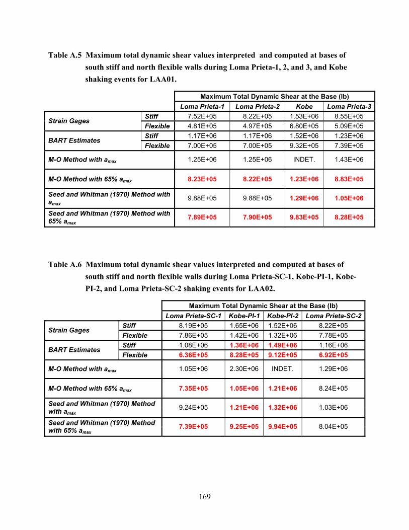
169
Table A.5 Maximum total dynamic shear values interpreted and computed at bases of south stiff and north flexible walls during Loma Prieta-1, 2, and 3, and Kobe shaking events for LAA01.
Maximum Total Dynamic Shear at the Base (lb) Loma Prieta-1 Loma Prieta-2 Kobe Loma Prieta-3
Stiff 7.52E+05 8.22E+05 1.53E+06 8.55E+05 Strain Gages Flexible 4.81E+05 4.97E+05 6.80E+05 5.09E+05 Stiff 1.17E+06 1.17E+06 1.52E+06 1.23E+06 BART Estimates Flexible 7.00E+05 7.00E+05 9.32E+05 7.39E+05
M-O Method with amax 1.25E+06 1.25E+06 INDET. 1.43E+06
M-O Method with 65% amax 8.23E+05 8.22E+05 1.23E+06 8.83E+05
Seed and Whitman (1970) Method with amax
9.88E+05 9.88E+05 1.29E+06 1.05E+06
Seed and Whitman (1970) Method with 65% amax
7.89E+05 7.90E+05 9.83E+05 8.28E+05
Table A.6 Maximum total dynamic shear values interpreted and computed at bases of south stiff and north flexible walls during Loma Prieta-SC-1, Kobe-PI-1, Kobe-PI-2, and Loma Prieta-SC-2 shaking events for LAA02.
Maximum Total Dynamic Shear at the Base (lb) Loma Prieta-SC-1 Kobe-PI-1 Kobe-PI-2 Loma Prieta-SC-2
Stiff 8.19E+05 1.65E+06 1.52E+06 8.22E+05 Strain Gages Flexible 7.86E+05 1.42E+06 1.32E+06 7.78E+05 Stiff 1.08E+06 1.36E+06 1.49E+06 1.16E+06 BART Estimates Flexible 6.36E+05 8.28E+05 9.12E+05 6.92E+05
M-O Method with amax 1.05E+06 2.30E+06 INDET. 1.29E+06
M-O Method with 65% amax 7.35E+05 1.05E+06 1.21E+06 8.24E+05
Seed and Whitman (1970) Method with amax
9.24E+05 1.21E+06 1.32E+06 1.03E+06
Seed and Whitman (1970) Method with 65% amax
7.39E+05 9.25E+05 9.94E+05 8.04E+05
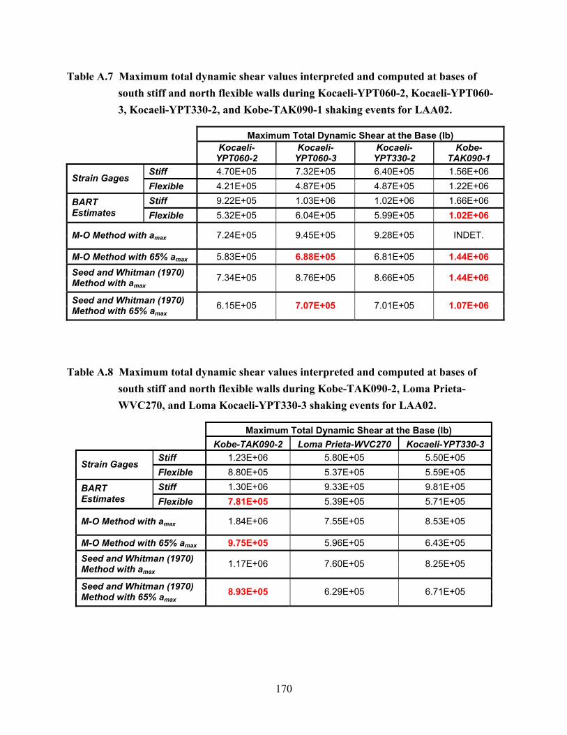
170
Table A.7 Maximum total dynamic shear values interpreted and computed at bases of south stiff and north flexible walls during Kocaeli-YPT060-2, Kocaeli-YPT060-3, Kocaeli-YPT330-2, and Kobe-TAK090-1 shaking events for LAA02.
Maximum Total Dynamic Shear at the Base (lb)
Kocaeli-
YPT060-2 Kocaeli-
YPT060-3 Kocaeli-
YPT330-2 Kobe-
TAK090-1 Stiff 4.70E+05 7.32E+05 6.40E+05 1.56E+06
Strain Gages Flexible 4.21E+05 4.87E+05 4.87E+05 1.22E+06 Stiff 9.22E+05 1.03E+06 1.02E+06 1.66E+06 BART
Estimates Flexible 5.32E+05 6.04E+05 5.99E+05 1.02E+06
M-O Method with amax 7.24E+05 9.45E+05 9.28E+05 INDET.
M-O Method with 65% amax 5.83E+05 6.88E+05 6.81E+05 1.44E+06 Seed and Whitman (1970) Method with amax
7.34E+05 8.76E+05 8.66E+05 1.44E+06
Seed and Whitman (1970) Method with 65% amax
6.15E+05 7.07E+05 7.01E+05 1.07E+06
Table A.8 Maximum total dynamic shear values interpreted and computed at bases of south stiff and north flexible walls during Kobe-TAK090-2, Loma Prieta-WVC270, and Loma Kocaeli-YPT330-3 shaking events for LAA02.
Maximum Total Dynamic Shear at the Base (lb) Kobe-TAK090-2 Loma Prieta-WVC270 Kocaeli-YPT330-3
Stiff 1.23E+06 5.80E+05 5.50E+05 Strain Gages
Flexible 8.80E+05 5.37E+05 5.59E+05 Stiff 1.30E+06 9.33E+05 9.81E+05 BART
Estimates Flexible 7.81E+05 5.39E+05 5.71E+05
M-O Method with amax 1.84E+06 7.55E+05 8.53E+05
M-O Method with 65% amax 9.75E+05 5.96E+05 6.43E+05
Seed and Whitman (1970) Method with amax
1.17E+06 7.60E+05 8.25E+05
Seed and Whitman (1970) Method with 65% amax
8.93E+05 6.29E+05 6.71E+05

171
Table A.9 Maximum dynamic moment increments measured and estimated at bases of south stiff and north flexible walls during Loma Prieta-1, 2, and 3, and Kobe shaking events for LAA01.
Maximum Dynamic Moment Increments at the Base (lb-in) Loma Prieta-1 Loma Prieta-2 Kobe Loma Prieta-3
Stiff 5.98E+07 6.38E+07 1.28E+08 6.45E+07 Strain Gages Flexible 3.30E+07 3.29E+07 5.64E+07 3.27E+07 Stiff 4.45E+07 4.89E+07 1.21E+08 4.48E+07 Force-Sensing Bolts Flexible 6.08E+07 5.99E+07 9.74E+07 5.61E+07 Stiff 6.25E+07 6.22E+07 1.14E+08 7.02E+07 BART Estimates Flexible 4.17E+07 4.14E+07 7.59E+07 4.68E+07
M-O Method with amax 6.20E+07 6.14E+07 INDET. 7.45E+07
M-O Method with 65% amax 3.00E+07 2.98E+07 6.04E+07 3.41E+07
Seed and Whitman (1970) Method with amax
8.44E+07 8.42E+07 1.28E+08 9.23E+07
Seed and Whitman (1970) Method with 65% amax
5.49E+07 5.47E+07 8.35E+07 6.00E+07
Table A.10 Maximum dynamic moment increments measured and estimated at bases of south stiff and north flexible walls during Loma Prieta-SC-1, Kobe-PI-1, Kobe-PI-2, and Loma Prieta-SC-2 shaking events for LAA02.
Maximum Dynamic Moment Increments at the Base (lb-in) Loma Prieta-SC-1 Kobe-PI-1 Kobe-PI-2 Loma Prieta-SC-2
Stiff 4.62E+07 1.08E+08 1.19E+08 6.47E+07 Strain Gages Flexible 2.46E+07 5.52E+07 8.11E+07 4.21E+07 Stiff 3.65E+07 1.20E+08 1.36E+08 5.09E+07 Force-Sensing Bolts Flexible 2.35E+07 6.88E+07 7.84E+07 4.00E+07 Stiff 5.35E+07 9.64E+07 1.15E+08 6.67E+07 BART Estimates Flexible 3.57E+07 6.43E+07 7.70E+07 4.45E+07
M-O Method with amax 4.90E+07 1.42E+08 INDET. 6.70E+07
M-O Method with 65% amax 2.52E+07 4.89E+07 6.07E+07 3.21E+07
Seed and Whitman (1970) Method with amax
7.85E+07 1.21E+08 1.37E+08 9.42E+07
Seed and Whitman (1970) Method with 65% amax
5.10E+07 7.88E+07 8.92E+07 6.13E+07
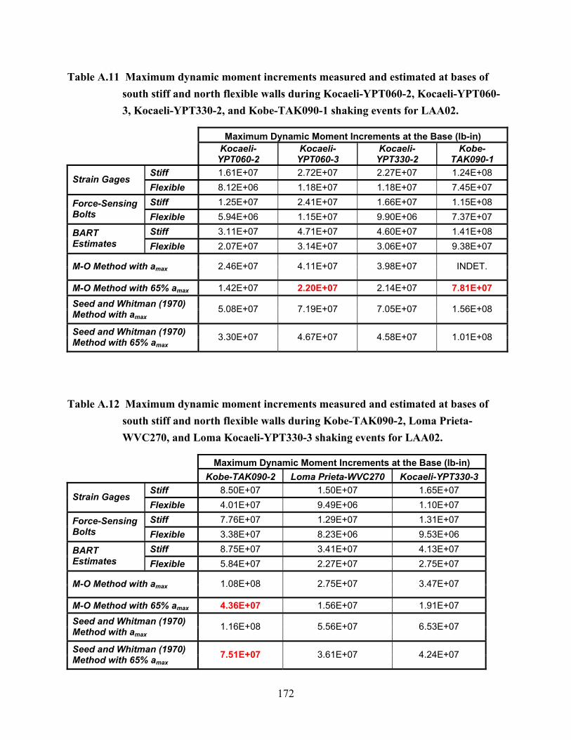
172
Table A.11 Maximum dynamic moment increments measured and estimated at bases of south stiff and north flexible walls during Kocaeli-YPT060-2, Kocaeli-YPT060-3, Kocaeli-YPT330-2, and Kobe-TAK090-1 shaking events for LAA02.
Maximum Dynamic Moment Increments at the Base (lb-in)
Kocaeli-
YPT060-2 Kocaeli-
YPT060-3 Kocaeli-
YPT330-2 Kobe-
TAK090-1 Stiff 1.61E+07 2.72E+07 2.27E+07 1.24E+08
Strain Gages Flexible 8.12E+06 1.18E+07 1.18E+07 7.45E+07 Stiff 1.25E+07 2.41E+07 1.66E+07 1.15E+08 Force-Sensing
Bolts Flexible 5.94E+06 1.15E+07 9.90E+06 7.37E+07 Stiff 3.11E+07 4.71E+07 4.60E+07 1.41E+08 BART
Estimates Flexible 2.07E+07 3.14E+07 3.06E+07 9.38E+07
M-O Method with amax 2.46E+07 4.11E+07 3.98E+07 INDET.
M-O Method with 65% amax 1.42E+07 2.20E+07 2.14E+07 7.81E+07 Seed and Whitman (1970) Method with amax
5.08E+07 7.19E+07 7.05E+07 1.56E+08
Seed and Whitman (1970) Method with 65% amax
3.30E+07 4.67E+07 4.58E+07 1.01E+08
Table A.12 Maximum dynamic moment increments measured and estimated at bases of south stiff and north flexible walls during Kobe-TAK090-2, Loma Prieta-WVC270, and Loma Kocaeli-YPT330-3 shaking events for LAA02.
Maximum Dynamic Moment Increments at the Base (lb-in) Kobe-TAK090-2 Loma Prieta-WVC270 Kocaeli-YPT330-3
Stiff 8.50E+07 1.50E+07 1.65E+07 Strain Gages
Flexible 4.01E+07 9.49E+06 1.10E+07 Stiff 7.76E+07 1.29E+07 1.31E+07 Force-Sensing
Bolts Flexible 3.38E+07 8.23E+06 9.53E+06 Stiff 8.75E+07 3.41E+07 4.13E+07 BART
Estimates Flexible 5.84E+07 2.27E+07 2.75E+07
M-O Method with amax 1.08E+08 2.75E+07 3.47E+07
M-O Method with 65% amax 4.36E+07 1.56E+07 1.91E+07
Seed and Whitman (1970) Method with amax
1.16E+08 5.56E+07 6.53E+07
Seed and Whitman (1970) Method with 65% amax
7.51E+07 3.61E+07 4.24E+07

PEER REPORTS
PEER reports are available from the National Information Service for Earthquake Engineering (NISEE). To order PEER reports, please contact the Pacific Earthquake Engineering Research Center, 1301 South 46th Street, Richmond, California 94804-4698. Tel.: (510) 665-3405; Fax: (510) 665-3420.
PEER 2007/06 Development of Improved Procedures for Seismic Design of Buried and Partially Buried Structures. Linda Al Atik and Nicholas Sitar. June 2007.
PEER 2007/05 Uncertainty and Correlation in Seismic Risk Assessment of Transportation Systems. Renee G. Lee and Anne S. Kiremidjian. July 2007.
PEER 2007/02 Campbell-Bozorgnia NGA Ground Motion Relations for the Geometric Mean Horizontal Component of Peak and Spectral Ground Motion Parameters. Kenneth W. Campbell and Yousef Bozorgnia. May 2007.
PEER 2007/01 Boore-Atkinson NGA Ground Motion Relations for the Geometric Mean Horizontal Component of Peak and Spectral Ground Motion Parameters. David M. Boore and Gail M. Atkinson. May. May 2007.
PEER 2006/12 Societal Implications of Performance-Based Earthquake Engineering. Peter J. May. May 2007.
PEER 2006/11 Probabilistic Seismic Demand Analysis Using Advanced Ground Motion Intensity Measures, Attenuation Relationships, and Near-Fault Effects. Polsak Tothong and C. Allin Cornell. March 2007.
PEER 2006/10 Application of the PEER PBEE Methodology to the I-880 Viaduct. Sashi Kunnath. February 2007.
PEER 2006/09 Quantifying Economic Losses from Travel Forgone Following a Large Metropolitan Earthquake. James Moore, Sungbin Cho, Yue Yue Fan, and Stuart Werner. November 2006.
PEER 2006/08 Vector-Valued Ground Motion Intensity Measures for Probabilistic Seismic Demand Analysis. Jack W. Baker and C. Allin Cornell. October 2006.
PEER 2006/07 Analytical Modeling of Reinforced Concrete Walls for Predicting Flexural and Coupled–Shear- Flexural Responses. Kutay Orakcal, Loenardo M. Massone, and John W. Wallace. October 2006.
PEER 2006/06 Nonlinear Analysis of a Soil-Drilled Pier System under Static and Dynamic Axial Loading. Gang Wang and Nicholas Sitar. November 2006.
PEER 2006/05 Advanced Seismic Assessment Guidelines. Paolo Bazzurro, C. Allin Cornell, Charles Menun, Maziar Motahari, and Nicolas Luco. September 2006.
PEER 2006/04 Probabilistic Seismic Evaluation of Reinforced Concrete Structural Components and Systems. Tae Hyung Lee and Khalid M. Mosalam. August 2006.
PEER 2006/03 Performance of Lifelines Subjected to Lateral Spreading. Scott A. Ashford and Teerawut Juirnarongrit. July 2006.
PEER 2006/02 Pacific Earthquake Engineering Research Center Highway Demonstration Project. Anne Kiremidjian, James Moore, Yue Yue Fan, Nesrin Basoz, Ozgur Yazali, and Meredith Williams. April 2006.
PEER 2006/01 Bracing Berkeley. A Guide to Seismic Safety on the UC Berkeley Campus. Mary C. Comerio, Stephen Tobriner, and Ariane Fehrenkamp. January 2006.
PEER 2005/16 Seismic Response and Reliability of Electrical Substation Equipment and Systems. Junho Song, Armen Der Kiureghian, and Jerome L. Sackman. April 2006.
PEER 2005/15 CPT-Based Probabilistic Assessment of Seismic Soil Liquefaction Initiation. R. E. S. Moss, R. B. Seed, R. E. Kayen, J. P. Stewart, and A. Der Kiureghian. April 2006.
PEER 2005/14 Workshop on Modeling of Nonlinear Cyclic Load-Deformation Behavior of Shallow Foundations. Bruce L. Kutter, Geoffrey Martin, Tara Hutchinson, Chad Harden, Sivapalan Gajan, and Justin Phalen. March 2006.
PEER 2005/13 Stochastic Characterization and Decision Bases under Time-Dependent Aftershock Risk in Performance-Based Earthquake Engineering. Gee Liek Yeo and C. Allin Cornell. July 2005.
PEER 2005/12 PEER Testbed Study on a Laboratory Building: Exercising Seismic Performance Assessment. Mary C. Comerio, editor. November 2005.
PEER 2005/11 Van Nuys Hotel Building Testbed Report: Exercising Seismic Performance Assessment. Helmut Krawinkler, editor. October 2005.
PEER 2005/10 First NEES/E-Defense Workshop on Collapse Simulation of Reinforced Concrete Building Structures. September 2005.

PEER 2005/09 Test Applications of Advanced Seismic Assessment Guidelines. Joe Maffei, Karl Telleen, Danya Mohr, William Holmes, and Yuki Nakayama. August 2006.
PEER 2005/08 Damage Accumulation in Lightly Confined Reinforced Concrete Bridge Columns. R. Tyler Ranf, Jared M. Nelson, Zach Price, Marc O. Eberhard, and John F. Stanton. April 2006.
PEER 2005/07 Experimental and Analytical Studies on the Seismic Response of Freestanding and Anchored Laboratory Equipment. Dimitrios Konstantinidis and Nicos Makris. January 2005.
PEER 2005/06 Global Collapse of Frame Structures under Seismic Excitations. Luis F. Ibarra and Helmut Krawinkler. September 2005.
PEER 2005//05 Performance Characterization of Bench- and Shelf-Mounted Equipment. Samit Ray Chaudhuri and Tara C. Hutchinson. May 2006.
PEER 2005/04 Numerical Modeling of the Nonlinear Cyclic Response of Shallow Foundations. Chad Harden, Tara Hutchinson, Geoffrey R. Martin, and Bruce L. Kutter. August 2005.
PEER 2005/03 A Taxonomy of Building Components for Performance-Based Earthquake Engineering. Keith A. Porter. September 2005.
PEER 2005/02 Fragility Basis for California Highway Overpass Bridge Seismic Decision Making. Kevin R. Mackie and Bozidar Stojadinovic. June 2005.
PEER 2005/01 Empirical Characterization of Site Conditions on Strong Ground Motion. Jonathan P. Stewart, Yoojoong Choi, and Robert W. Graves. June 2005.
PEER 2004/09 Electrical Substation Equipment Interaction: Experimental Rigid Conductor Studies. Christopher Stearns and André Filiatrault. February 2005.
PEER 2004/08 Seismic Qualification and Fragility Testing of Line Break 550-kV Disconnect Switches. Shakhzod M. Takhirov, Gregory L. Fenves, and Eric Fujisaki. January 2005.
PEER 2004/07 Ground Motions for Earthquake Simulator Qualification of Electrical Substation Equipment. Shakhzod M. Takhirov, Gregory L. Fenves, Eric Fujisaki, and Don Clyde. January 2005.
PEER 2004/06 Performance-Based Regulation and Regulatory Regimes. Peter J. May and Chris Koski. September 2004.
PEER 2004/05 Performance-Based Seismic Design Concepts and Implementation: Proceedings of an International Workshop. Peter Fajfar and Helmut Krawinkler, editors. September 2004.
PEER 2004/04 Seismic Performance of an Instrumented Tilt-up Wall Building. James C. Anderson and Vitelmo V. Bertero. July 2004.
PEER 2004/03 Evaluation and Application of Concrete Tilt-up Assessment Methodologies. Timothy Graf and James O. Malley. October 2004.
PEER 2004/02 Analytical Investigations of New Methods for Reducing Residual Displacements of Reinforced Concrete Bridge Columns. Junichi Sakai and Stephen A. Mahin. August 2004.
PEER 2004/01 Seismic Performance of Masonry Buildings and Design Implications. Kerri Anne Taeko Tokoro, James C. Anderson, and Vitelmo V. Bertero. February 2004.
PEER 2003/18 Performance Models for Flexural Damage in Reinforced Concrete Columns. Michael Berry and Marc Eberhard. August 2003.
PEER 2003/17 Predicting Earthquake Damage in Older Reinforced Concrete Beam-Column Joints. Catherine Pagni and Laura Lowes. October 2004.
PEER 2003/16 Seismic Demands for Performance-Based Design of Bridges. Kevin Mackie and Bo!idar Stojadinovic. August 2003.
PEER 2003/15 Seismic Demands for Nondeteriorating Frame Structures and Their Dependence on Ground Motions. Ricardo Antonio Medina and Helmut Krawinkler. May 2004.
PEER 2003/14 Finite Element Reliability and Sensitivity Methods for Performance-Based Earthquake Engineering. Terje Haukaas and Armen Der Kiureghian. April 2004.
PEER 2003/13 Effects of Connection Hysteretic Degradation on the Seismic Behavior of Steel Moment-Resisting Frames. Janise E. Rodgers and Stephen A. Mahin. March 2004.
PEER 2003/12 Implementation Manual for the Seismic Protection of Laboratory Contents: Format and Case Studies. William T. Holmes and Mary C. Comerio. October 2003.
PEER 2003/11 Fifth U.S.-Japan Workshop on Performance-Based Earthquake Engineering Methodology for Reinforced Concrete Building Structures. February 2004.

PEER 2003/10 A Beam-Column Joint Model for Simulating the Earthquake Response of Reinforced Concrete Frames. Laura N. Lowes, Nilanjan Mitra, and Arash Altoontash. February 2004.
PEER 2003/09 Sequencing Repairs after an Earthquake: An Economic Approach. Marco Casari and Simon J. Wilkie. April 2004.
PEER 2003/08 A Technical Framework for Probability-Based Demand and Capacity Factor Design (DCFD) Seismic Formats. Fatemeh Jalayer and C. Allin Cornell. November 2003.
PEER 2003/07 Uncertainty Specification and Propagation for Loss Estimation Using FOSM Methods. Jack W. Baker and C. Allin Cornell. September 2003.
PEER 2003/06 Performance of Circular Reinforced Concrete Bridge Columns under Bidirectional Earthquake Loading. Mahmoud M. Hachem, Stephen A. Mahin, and Jack P. Moehle. February 2003.
PEER 2003/05 Response Assessment for Building-Specific Loss Estimation. Eduardo Miranda and Shahram Taghavi. September 2003.
PEER 2003/04 Experimental Assessment of Columns with Short Lap Splices Subjected to Cyclic Loads. Murat Melek, John W. Wallace, and Joel Conte. April 2003.
PEER 2003/03 Probabilistic Response Assessment for Building-Specific Loss Estimation. Eduardo Miranda and Hesameddin Aslani. September 2003.
PEER 2003/02 Software Framework for Collaborative Development of Nonlinear Dynamic Analysis Program. Jun Peng and Kincho H. Law. September 2003.
PEER 2003/01 Shake Table Tests and Analytical Studies on the Gravity Load Collapse of Reinforced Concrete Frames. Kenneth John Elwood and Jack P. Moehle. November 2003.
PEER 2002/24 Performance of Beam to Column Bridge Joints Subjected to a Large Velocity Pulse. Natalie Gibson, André Filiatrault, and Scott A. Ashford. April 2002.
PEER 2002/23 Effects of Large Velocity Pulses on Reinforced Concrete Bridge Columns. Greg L. Orozco and Scott A. Ashford. April 2002.
PEER 2002/22 Characterization of Large Velocity Pulses for Laboratory Testing. Kenneth E. Cox and Scott A. Ashford. April 2002.
PEER 2002/21 Fourth U.S.-Japan Workshop on Performance-Based Earthquake Engineering Methodology for Reinforced Concrete Building Structures. December 2002.
PEER 2002/20 Barriers to Adoption and Implementation of PBEE Innovations. Peter J. May. August 2002.
PEER 2002/19 Economic-Engineered Integrated Models for Earthquakes: Socioeconomic Impacts. Peter Gordon, James E. Moore II, and Harry W. Richardson. July 2002.
PEER 2002/18 Assessment of Reinforced Concrete Building Exterior Joints with Substandard Details. Chris P. Pantelides, Jon Hansen, Justin Nadauld, and Lawrence D. Reaveley. May 2002.
PEER 2002/17 Structural Characterization and Seismic Response Analysis of a Highway Overcrossing Equipped with Elastomeric Bearings and Fluid Dampers: A Case Study. Nicos Makris and Jian Zhang. November 2002.
PEER 2002/16 Estimation of Uncertainty in Geotechnical Properties for Performance-Based Earthquake Engineering. Allen L. Jones, Steven L. Kramer, and Pedro Arduino. December 2002.
PEER 2002/15 Seismic Behavior of Bridge Columns Subjected to Various Loading Patterns. Asadollah Esmaeily-Gh. and Yan Xiao. December 2002.
PEER 2002/14 Inelastic Seismic Response of Extended Pile Shaft Supported Bridge Structures. T.C. Hutchinson, R.W. Boulanger, Y.H. Chai, and I.M. Idriss. December 2002.
PEER 2002/13 Probabilistic Models and Fragility Estimates for Bridge Components and Systems. Paolo Gardoni, Armen Der Kiureghian, and Khalid M. Mosalam. June 2002.
PEER 2002/12 Effects of Fault Dip and Slip Rake on Near-Source Ground Motions: Why Chi-Chi Was a Relatively Mild M7.6 Earthquake. Brad T. Aagaard, John F. Hall, and Thomas H. Heaton. December 2002.
PEER 2002/11 Analytical and Experimental Study of Fiber-Reinforced Strip Isolators. James M. Kelly and Shakhzod M. Takhirov. September 2002.
PEER 2002/10 Centrifuge Modeling of Settlement and Lateral Spreading with Comparisons to Numerical Analyses. Sivapalan Gajan and Bruce L. Kutter. January 2003.
PEER 2002/09 Documentation and Analysis of Field Case Histories of Seismic Compression during the 1994 Northridge, California, Earthquake. Jonathan P. Stewart, Patrick M. Smith, Daniel H. Whang, and Jonathan D. Bray. October 2002.

PEER 2002/08 Component Testing, Stability Analysis and Characterization of Buckling-Restrained Unbonded BracesTM. Cameron Black, Nicos Makris, and Ian Aiken. September 2002.
PEER 2002/07 Seismic Performance of Pile-Wharf Connections. Charles W. Roeder, Robert Graff, Jennifer Soderstrom, and Jun Han Yoo. December 2001.
PEER 2002/06 The Use of Benefit-Cost Analysis for Evaluation of Performance-Based Earthquake Engineering Decisions. Richard O. Zerbe and Anthony Falit-Baiamonte. September 2001.
PEER 2002/05 Guidelines, Specifications, and Seismic Performance Characterization of Nonstructural Building Components and Equipment. André Filiatrault, Constantin Christopoulos, and Christopher Stearns. September 2001.
PEER 2002/04 Consortium of Organizations for Strong-Motion Observation Systems and the Pacific Earthquake Engineering Research Center Lifelines Program: Invited Workshop on Archiving and Web Dissemination of Geotechnical Data, 4–5 October 2001. September 2002.
PEER 2002/03 Investigation of Sensitivity of Building Loss Estimates to Major Uncertain Variables for the Van Nuys Testbed. Keith A. Porter, James L. Beck, and Rustem V. Shaikhutdinov. August 2002.
PEER 2002/02 The Third U.S.-Japan Workshop on Performance-Based Earthquake Engineering Methodology for Reinforced Concrete Building Structures. July 2002.
PEER 2002/01 Nonstructural Loss Estimation: The UC Berkeley Case Study. Mary C. Comerio and John C. Stallmeyer. December 2001.
PEER 2001/16 Statistics of SDF-System Estimate of Roof Displacement for Pushover Analysis of Buildings. Anil K. Chopra, Rakesh K. Goel, and Chatpan Chintanapakdee. December 2001.
PEER 2001/15 Damage to Bridges during the 2001 Nisqually Earthquake. R. Tyler Ranf, Marc O. Eberhard, and Michael P. Berry. November 2001.
PEER 2001/14 Rocking Response of Equipment Anchored to a Base Foundation. Nicos Makris and Cameron J. Black. September 2001.
PEER 2001/13 Modeling Soil Liquefaction Hazards for Performance-Based Earthquake Engineering. Steven L. Kramer and Ahmed-W. Elgamal. February 2001.
PEER 2001/12 Development of Geotechnical Capabilities in OpenSees. Boris Jeremi . September 2001.
PEER 2001/11 Analytical and Experimental Study of Fiber-Reinforced Elastomeric Isolators. James M. Kelly and Shakhzod M. Takhirov. September 2001.
PEER 2001/10 Amplification Factors for Spectral Acceleration in Active Regions. Jonathan P. Stewart, Andrew H. Liu, Yoojoong Choi, and Mehmet B. Baturay. December 2001.
PEER 2001/09 Ground Motion Evaluation Procedures for Performance-Based Design. Jonathan P. Stewart, Shyh-Jeng Chiou, Jonathan D. Bray, Robert W. Graves, Paul G. Somerville, and Norman A. Abrahamson. September 2001.
PEER 2001/08 Experimental and Computational Evaluation of Reinforced Concrete Bridge Beam-Column Connections for Seismic Performance. Clay J. Naito, Jack P. Moehle, and Khalid M. Mosalam. November 2001.
PEER 2001/07 The Rocking Spectrum and the Shortcomings of Design Guidelines. Nicos Makris and Dimitrios Konstantinidis. August 2001.
PEER 2001/06 Development of an Electrical Substation Equipment Performance Database for Evaluation of Equipment Fragilities. Thalia Agnanos. April 1999.
PEER 2001/05 Stiffness Analysis of Fiber-Reinforced Elastomeric Isolators. Hsiang-Chuan Tsai and James M. Kelly. May 2001.
PEER 2001/04 Organizational and Societal Considerations for Performance-Based Earthquake Engineering. Peter J. May. April 2001.
PEER 2001/03 A Modal Pushover Analysis Procedure to Estimate Seismic Demands for Buildings: Theory and Preliminary Evaluation. Anil K. Chopra and Rakesh K. Goel. January 2001.
PEER 2001/02 Seismic Response Analysis of Highway Overcrossings Including Soil-Structure Interaction. Jian Zhang and Nicos Makris. March 2001.
PEER 2001/01 Experimental Study of Large Seismic Steel Beam-to-Column Connections. Egor P. Popov and Shakhzod M. Takhirov. November 2000.
PEER 2000/10 The Second U.S.-Japan Workshop on Performance-Based Earthquake Engineering Methodology for Reinforced Concrete Building Structures. March 2000.

PEER 2000/09 Structural Engineering Reconnaissance of the August 17, 1999 Earthquake: Kocaeli (Izmit), Turkey. Halil Sezen, Kenneth J. Elwood, Andrew S. Whittaker, Khalid Mosalam, John J. Wallace, and John F. Stanton. December 2000.
PEER 2000/08 Behavior of Reinforced Concrete Bridge Columns Having Varying Aspect Ratios and Varying Lengths of Confinement. Anthony J. Calderone, Dawn E. Lehman, and Jack P. Moehle. January 2001.
PEER 2000/07 Cover-Plate and Flange-Plate Reinforced Steel Moment-Resisting Connections. Taejin Kim, Andrew S. Whittaker, Amir S. Gilani, Vitelmo V. Bertero, and Shakhzod M. Takhirov. September 2000.
PEER 2000/06 Seismic Evaluation and Analysis of 230-kV Disconnect Switches. Amir S. J. Gilani, Andrew S. Whittaker, Gregory L. Fenves, Chun-Hao Chen, Henry Ho, and Eric Fujisaki. July 2000.
PEER 2000/05 Performance-Based Evaluation of Exterior Reinforced Concrete Building Joints for Seismic Excitation. Chandra Clyde, Chris P. Pantelides, and Lawrence D. Reaveley. July 2000.
PEER 2000/04 An Evaluation of Seismic Energy Demand: An Attenuation Approach. Chung-Che Chou and Chia-Ming Uang. July 1999.
PEER 2000/03 Framing Earthquake Retrofitting Decisions: The Case of Hillside Homes in Los Angeles. Detlof von Winterfeldt, Nels Roselund, and Alicia Kitsuse. March 2000.
PEER 2000/02 U.S.-Japan Workshop on the Effects of Near-Field Earthquake Shaking. Andrew Whittaker, ed. July 2000.
PEER 2000/01 Further Studies on Seismic Interaction in Interconnected Electrical Substation Equipment. Armen Der Kiureghian, Kee-Jeung Hong, and Jerome L. Sackman. November 1999.
PEER 1999/14 Seismic Evaluation and Retrofit of 230-kV Porcelain Transformer Bushings. Amir S. Gilani, Andrew S. Whittaker, Gregory L. Fenves, and Eric Fujisaki. December 1999.
PEER 1999/13 Building Vulnerability Studies: Modeling and Evaluation of Tilt-up and Steel Reinforced Concrete Buildings. John W. Wallace, Jonathan P. Stewart, and Andrew S. Whittaker, editors. December 1999.
PEER 1999/12 Rehabilitation of Nonductile RC Frame Building Using Encasement Plates and Energy-Dissipating Devices. Mehrdad Sasani, Vitelmo V. Bertero, James C. Anderson. December 1999.
PEER 1999/11 Performance Evaluation Database for Concrete Bridge Components and Systems under Simulated Seismic Loads. Yael D. Hose and Frieder Seible. November 1999.
PEER 1999/10 U.S.-Japan Workshop on Performance-Based Earthquake Engineering Methodology for Reinforced Concrete Building Structures. December 1999.
PEER 1999/09 Performance Improvement of Long Period Building Structures Subjected to Severe Pulse-Type Ground Motions. James C. Anderson, Vitelmo V. Bertero, and Raul Bertero. October 1999.
PEER 1999/08 Envelopes for Seismic Response Vectors. Charles Menun and Armen Der Kiureghian. July 1999.
PEER 1999/07 Documentation of Strengths and Weaknesses of Current Computer Analysis Methods for Seismic Performance of Reinforced Concrete Members. William F. Cofer. November 1999.
PEER 1999/06 Rocking Response and Overturning of Anchored Equipment under Seismic Excitations. Nicos Makris and Jian Zhang. November 1999.
PEER 1999/05 Seismic Evaluation of 550 kV Porcelain Transformer Bushings. Amir S. Gilani, Andrew S. Whittaker, Gregory L. Fenves, and Eric Fujisaki. October 1999.
PEER 1999/04 Adoption and Enforcement of Earthquake Risk-Reduction Measures. Peter J. May, Raymond J. Burby, T. Jens Feeley, and Robert Wood.
PEER 1999/03 Task 3 Characterization of Site Response General Site Categories. Adrian Rodriguez-Marek, Jonathan D. Bray, and Norman Abrahamson. February 1999.
PEER 1999/02 Capacity-Demand-Diagram Methods for Estimating Seismic Deformation of Inelastic Structures: SDF Systems. Anil K. Chopra and Rakesh Goel. April 1999.
PEER 1999/01 Interaction in Interconnected Electrical Substation Equipment Subjected to Earthquake Ground Motions. Armen Der Kiureghian, Jerome L. Sackman, and Kee-Jeung Hong. February 1999.
PEER 1998/08 Behavior and Failure Analysis of a Multiple-Frame Highway Bridge in the 1994 Northridge Earthquake. Gregory L. Fenves and Michael Ellery. December 1998.
PEER 1998/07 Empirical Evaluation of Inertial Soil-Structure Interaction Effects. Jonathan P. Stewart, Raymond B. Seed, and Gregory L. Fenves. November 1998.
PEER 1998/06 Effect of Damping Mechanisms on the Response of Seismic Isolated Structures. Nicos Makris and Shih-Po Chang. November 1998.

PEER 1998/05 Rocking Response and Overturning of Equipment under Horizontal Pulse-Type Motions. Nicos Makris and Yiannis Roussos. October 1998.
PEER 1998/04 Pacific Earthquake Engineering Research Invitational Workshop Proceedings, May 14–15, 1998: Defining the Links between Planning, Policy Analysis, Economics and Earthquake Engineering. Mary Comerio and Peter Gordon. September 1998.
PEER 1998/03 Repair/Upgrade Procedures for Welded Beam to Column Connections. James C. Anderson and Xiaojing Duan. May 1998.
PEER 1998/02 Seismic Evaluation of 196 kV Porcelain Transformer Bushings. Amir S. Gilani, Juan W. Chavez, Gregory L. Fenves, and Andrew S. Whittaker. May 1998.
PEER 1998/01 Seismic Performance of Well-Confined Concrete Bridge Columns. Dawn E. Lehman and Jack P. Moehle. December 2000.

ONLINE REPORTS
The following PEER reports are available by Internet only at http://peer.berkeley.edu/publications/peer_reports.html
PEER 2007/101 Generalized Hybrid Simulation Framework for Structural Systems Subjected to Seismic Loading. Tarek Elkhoraibi and Khalid M. Mosalam. July 2007.
PEER 2007/100 Seismic Evaluation of Reinforced Concrete Buildings Including Effects of Masonry Infill Walls. Alidad Hashemi and Khalid M. Mosalam. July 2007.


