NPS ARCHIVE
1964 ^1KH1GMAN, P Jfc&
HRI
111
$$W$#$$fyi IBB1^^^^fifll
ROOT LOCUS TECHNIQUES IN THE LOS S PLANSFOR DESIGN AND ANALYSIS OFFEEDBACK CONTROL SYSTEMS
DALE R. KLUGMAN
SMiilliSIS;Wmm
"'''*, .',-1 as
' • H9S :
' Ed ' .
"'' '
• <i >:
'
:
1HHHH!&mWm
C-iWW

DUDLEY KNOX LIBRARY
NAVAL POSTGRADUATE SCHOOL
MONTEREY CA 93943-5101
mm*n$. NA"VAl POSTGRADUATE SCHOOT
MONTEREY, CALIFORNIA


ROOT LOCUS TECHNIQUES IN THE LOG S PLANE
FOR DESIGN AND ANALYSIS OF FEEDBACK CONTROL SYSTEMS
******
Dale R. Klugman


05. NAVAL P D'.iATF SCH0<3L
ROOT LOCUS TECHNIQUES IN THE LOG S PLANE
FOR DESIGN AND ANALYSIS OF FEEDBACK CONTROL SYSTEMS
by
Dale R. Klugman
Lieutenant, United States Navy
Submitted in partial fulfillment ofthe requirements for the degree of
MASTER OF SCIENCEIN
ELECTRICAL ENGINEERING
United States Naval Postgraduate SchoolMonterey, California
19 6 4


Library
u.s. naval postgraduate schoolmonterey, california "
ROOT LOCUS TECHNIQUES IN THE LOG S PLANE
FOR DESIGN AND ANALYSIS OF FEEDBACK CONTROL SYSTEMS
by
Dale R. Klugman
This work is accepted as fulfilling
the thesis requirements for the degree of
MASTER OF SCIENCE
IN
ELECTRICAL ENGINEERING
from the
United States Naval Postgraduate School

ABSTRACT
Root locus plots in the s plane are practically limited to a span of
two decades. In problems where some poles are very close to the origin,
while other poles or zeros are at very large values of s, sufficient
resolution of the locus may not be available in two decades of the s plane.
However, root loci can be plotted in the In s_ plane using as many decades
as desired (and whichever are desired).
Electro-Scientific Industries Corporation manufactures an analog com-
puter, THE ESIAC, which constructs root locus plots in the In s plane.
This paper presents a mathematical analysis of the In s plane, a simple
method of plotting root loci in the In s plane, and several practical
examples demonstrating the technique. Construction of root loci by this
method requires the use of one template.
ii


TABLE OF CONTENTS
Chapter Title Page
I Plotting in the In s plane
1. Introduction 1
2. The In s plane 1
3. The general line 4
4. Justification 7
5. Plotting root loci 10
6. Summary 13
II Application to sensitivity design
1. Sensitivity design in the s plane 14
2. Sensitivity design in the In s plane 16
3. Design example 16
4. Summary 18
III Compensation design example
1. Compensation 20
2. Frequency response 21
3. Transient response 22
IV Factoring a polynomial
1. One real root, one pair of complex-conjugate roots 24
2. Two pair of complex- conjugate roots 24
V Conclusion and appendices
1. Conclusion 27
2. Illustrations 28
3. Bibliography 46
iii


LIST OF ILLUSTRATIONS
Figure Page
1. The w plane 28
2. Four decades of the s plane 29
3. Four decades of the w plane 30
4. Selected lines mapped on w plane 31
5. The general line in the s plane 32
6. The template 33
7. Sensitivity vector diagram 3A
8. Plant singularities and desired rootin w plane 35
9. Sensitivity design vector diagram 36
10. Root locus plot of uncompensated plantin w plane 37
11. Root locus plot of compensated plantin w plane 38
12. Bode diagram of uncompensated plant 40
13. Bode diagram of compensated plant 41
14. Root locus solution of third-orderpolynomial 43
15. Root locus solution of polynomial 44
16. Root locus solution of fourth-orderpolynomial 45
IV


TABLE OF SYMBOLS AND ABBREVIATIONS
s - the complex variable
V~ - the real part of s
LO - the imaginary part of s
In - logarithm to the base e
w - complex variable •=. In s
u - the real part of w
v - the imaginary part of w
|s| - the magnitude of s
& - the argument of s
CO - infinity
m - parameter (slope)
b - parameter (intercept)
O - the length of the "perpendicular radial"
G< - angle of inclination of the general line, Fig. 5
p- template scale reading at point one
p„ - template scale reading at point two
K - template scale multiplier
1 - the number of poles
n - the number of zeros
r - indexing number
^7~~ - the centroid of asymptotes
k - open loop gain (transient response form)
P - pole
Z - zero

U- factor multiplication symbol (as 251 means summation)
v^. - root gain sensitivityk
q. - the root in question
L - the loop gain
7 - partial derivative
EL - definition or identity sign
O- ~ root-zero sensitivity
z. - zero in question
£\* - root-pole sensitivity
p. - pole in question
U - length and phase reference vector for pole and zerosensitivities
Kf
- open loop gain (frequency response form)
a> - phase shift of compensator
UOt- imaginary part of dominant root q
p - pole of compensator
z - zero of compensator
R(s) - LaPlace Transform of input function
C(s) - LaPlace Transform of output function
G(s) - LaPlace Transform of open loop transfer function
C(t) - time response of output
C. - constants
u(t) - unit step function
vi


PLOTTING IN THE LOG S PLANE
1. Introduction
The value of root locus plotting is limited in those applications
where some poles and zeros are widely separated and others are close to
the origin or close to each other. When scale is expanded to show suffi-
cient detail close to the origin, other poles are moved off the paper.
The designer needs to see all the poles and zeros, yet retain sufficient
detail near the origin.
Logarithmic sea] ing solves the problem. This paper examines the
properties of the In s plane and then shows how each root locus sketching/
plotting technique in linear coordinates (s plane) also applies in the
In s plane. In the s plane, all the present root locus technique is
based upon straight lines, slopes, and lengths. Hence, an analogous
procedure requires the In s plane equivalent of a straight line, slope,
and length.
2. The In s plane
The s plane is defined by the rectangular coordinates s=-^_-//' a^
and the polar coordinates 5 = \s\ ZLQ . The In s plane, hereinafter
denoted by w, shall be defined by rectangular coordinates w = u + jv.
The conformal mapping relation between the planes is then
w = u + jv ln(s) = In /si + j& . Hence, equating reals and imagin-
aries:
u - In /s/
v = eand

Thus the ordinate of the w plane measures © and the abscissa
measures In | s | . Referring to Fig. 1, the w plane, note that © extends
from -00 to +00, corresponding to more than one polar coordinate revolu-
tion in the s plane. Therefore, every point on the s plane is repre-
sented, in one to one correspondence in the w plane, in the infinite
strip bounded by — & == 2.JT . Hence, this strip provides single
valued correspondence.
The scales of e and In fs| are equal. This choice was made to
retain the properties of conformal mapping. The abscissa is linearly
calibrated in In | s | with one unit of In jsj equal in length to one
radian of the ordinate. Then a logarithmic scale division calibrates the
abscissa directly in /s/ . This is a most important point; for by using
four-cycle semi-log paper, any four decades of e vs /sj may be plotted.
The cross-hatched area on Fig. 1 depicts such an area, and corresponds
to the cross-hatched area on the s plane shown in Fig. 2.
Fig. 3 shows this same area on a full-sized sheet of semi-log paper.
The horizontal lines ( = constant) represent radial lines through the
origin of the s plane; the vertical lines ( js( constant) must repre-
sent circles around the origin of the s plane. In the s plane, any radial
line can be calibrated in length by the family of circles about the
origin, /s / = 1, 2, ... CO, Hence, the horizontal lines in the w plane
are calibrated in length by the vertical lines, /s/ 1, 2, »• • OO
Summarizing, the semi- log paper provides all the s plane radial lines,
already calibrated in length. Further, the slope of these radial lines is
the ordinate scale.
To analyze the general line, not passing through the origin, examina-
tion of the relation between Gartesian coordinates, v-, uJ and u, v,


shows that
:
W = /n (5)
v~-f^ = e e^ - & (cos v + ^'° v
Equating real and imaginary terms:
v = e^ ^s v(A
In (T) - u -h In. cos v/„^ t= a + In Sin v
These relations define families of transcendental curves represent-
ing the vertical and horizontal lines of the s plane. Fig. 4 shows these
families in the w plane, covering the same four decades as Figs. 1, 2,
and 3. The w plane vertical and horizontal lines have been omitted for
clarity, but the scales are present. Selected members of the family have
been labeled in "s plane counterpart" notation for easy reference.
Notice that the form of all the curves is identical. Examine the
three curves: v~ :=. — O t£~ T~— ~L V~— -2, Change in the value of
V~~ shifts the curve laterally. Reference to the defining equation shows
this effect. Here, In \r~ is an arbitrary constant. Changing its value
changes the value of u, equally, throughout the length of the curve.
Next examine the curves UJ — -r / and uJ — -t- £. . The same lateral
shift occurs as between V~ — -/
o.nal V~ ~ — 2.. This observation is
expected from the defining equation In u> — u -j- I n Sin V and
hence, ul-=. lh lo — In sin \/ . This effect is generalized
below.
At this point it is well to note that a term In v with V taking on

negative values is really not a cause for concern. In the s plane,
InC+v- ) is a positive distance measured along the & line and
ln(-V ) is a positive distance measured along the & = -180 line, pro-
viding the correct minus sign.
Before moving to the general line, ^.laj =- nn T~ -h u?
some helpful geometric properties should be examined. In the s plane,
the family of lines LU=.-ao.»,-IO-hl2., . . i~ CJO
are all symmetric about the line V~= which is the ^uJ axis. The
family of lines V"~ — -CO. .. —A Of+l
f2.
}, > > + OO are
all symmetric about the line LO - 0, the horizontal axis. Thus a line
of symmetry is a line drawn from the origin, perpendicular to the line
in question. Since angles are preserved in conformal mapping, we expect
these same families of lines (e.g. V" s £>/-/
).,,—oo) to be symmetrical
about their respective perpendicular radials (e.g. UJ - 0) in the w plane.
Reference to Fig. 4 provides confirmation.
3. The general line
Let the general line (not through the origin) in the s plane be
LO — rn V" -f t) • Fig. 5 shows such a line. Define the
perpendicular from the origin to this line: "the perpendicular radial,"
and the length of the perpendicular radial "d." The radial parallel to
UJ =. ry> V~ -h t) (i.e. UJ - /-n V" ) is defined: "the parallel
radial."
"Slote: The line (W = 0) is the same line as (O - 0, 180°, 360°)


UO -=. nn v~ 4- b
6 S/n v/ — me COz>v -h b
Q."" (sin v— tfncos v) =b £>
but /9^ — "Zr^^J <A where ri angle of inclination of line
But UL -h I n S lh V ZZ. I n L*-> is the transformation equation
for the cartesian coordinate lines. Hence: the transcendental curves
corresponding to all the straight lines in the s plane, not passing
through the origin, have the same form as the Cartesian coordinate
(vertical and horizontal) lines. Hence, the shape is the same, and they
differ only in positioning. Therefore, one template may be used to draw
any non-radial straight line provided adequate rules for positioning it
are developed.
Fig. 6 illustrates such a template. The template represents every
non-radial straight line, mapped onto w, just as surely as the edge of a
triangle or T-square represents every straight line in the s plane.
For clarity, rules for positioning the template, reading slope, and
reading length are listed now, with proofs to follow in the next section:
a. The template is always used in the same orientation, with the

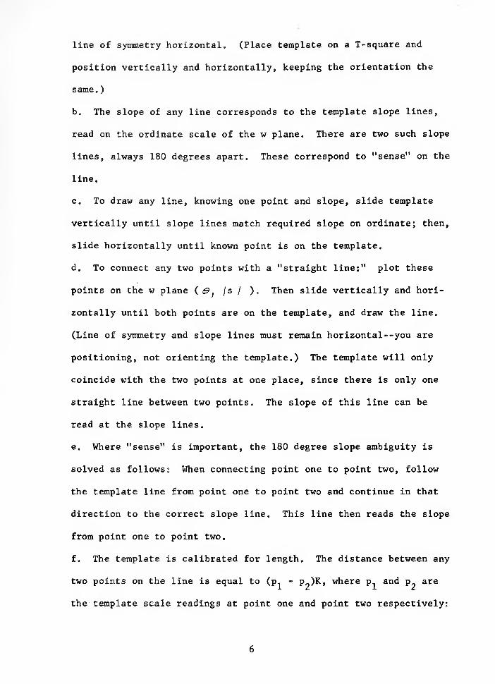
line of symmetry horizontal. (Place template on a T-square and
position vertically and horizontally, keeping the orientation the
same.)
b. The slope of any line corresponds to the template slope lines,
read on the ordinate scale of the w plane. There are two such slope
lines, always 180 degrees apart. These correspond to "sense" on the
line.
c. To draw any line, knowing one point and slope, slide template
vertically until slope lines match required slope on ordinate; then,
slide horizontally until known point is on the template.
d. To connect any two points with a "straight line:" plot these
points on the w plane ( &)
/s / ). Then slide vertically and hori-
zontally until both points are on the template, and draw the line.
(Line of symmetry and slope lines must remain horizontal--you are
positioning, not orienting the template.) The template will only
coincide with the two points at one place, since there is only one
straight line between two points. The slope of this line can be
read at the slope lines.
e. Where "sense" is important, the 180 degree slope ambiguity is
solved as follows: When connecting point one to point two, follow
the template line from point one to point two and continue in that
direction to the correct slope line. This line then reads the slope
from point one to point two.
f. The template is calibrated for length. The distance between any
two points on the line is equal to (p1
- P 9)K, where p and p are
the template scale readings at point one and point two respectively:


and K is a scale multiplier, varying with the length of the per-
pendicular radial. Values of K can be read directly on the|s/
scale at the template arrow.
Using this template, straight lines, slopes, and lengths can be
plotted as quickly on the w plane as a ruler and protracter plot them
on the s plane.
4. Justification (casual reader may skip)
The w plane equation of the general straight line is
ul -f In (sln(v-*)) — fh (& ccs cxj
= lh a cos rfj- lh(sinW-4
Recall: UL — hi lA-J — lh ( £ in vj was an equation of cartesian co-
ordinates, and changes in laj shifted the curve laterally only. In the
general equation, lh ( b co^ca) corresponds to In UJ . (b and cK
are constants for a given line.) Changing b will have the same qualita-
tive effect as changing uU , i.e. shifting the curve laterally.
Referring to Fig. 5, note D cos <^~ O. Hence:
U. — ci — I h ( 5 m ( V ~ (a)J , It has just been shown how, by
moving b, d is changed and the curve is shifted horizontally. Now, hold
d fixed and change the slope (or c< ). Recall the Cartesian defining
equations for vertical and horizontal lines:
UL = lh V ~ lh (Cd v) <**cl
u - lhu> - lh(S/»v) = //, us - lft(cos(V --g)J
When d is held fixed and these two are compared, V" — UJ, and the
only difference is the (p{ term (X — O &hc/ <A — -h ^2,
And it has been previously shown in Fig. 4 that this corresponded to a
vertical shift of 90 degrees only. Hence, varying any parameter shifts

the curves position only.
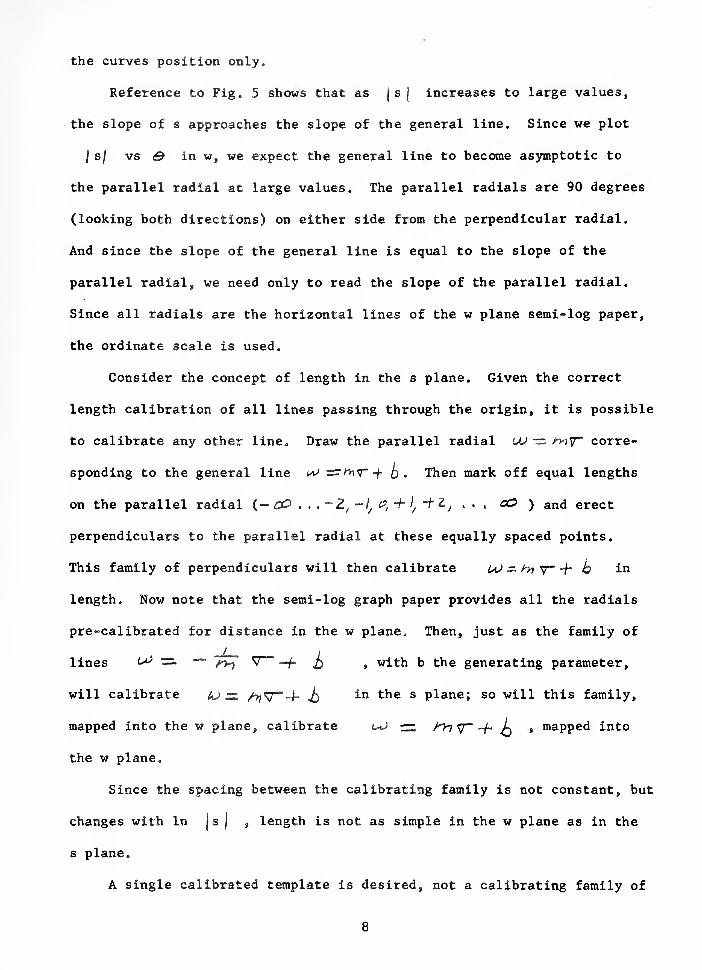
Reference to Fig. 5 shows that as |sj increases to large values,
the slope of s approaches the slope of the general line. Since we plot
Isj vs O in w, we expect the general line to become asymptotic to
the parallel radial at large values. The parallel radials are 90 degrees
(looking both directions) on either side from the perpendicular radial.
And since the slope of the general line is equal to the slope of the
parallel radial, we need only to read the slope of the parallel radial.
Since all radials are the horizontal lines of the w plane semi-log paper,
the ordinate scale is used.
Consider the concept of length in the s plane. Given the correct
length calibration of all lines passing through the origin, it is possible
to calibrate any other line. Draw the parallel radial UU — my~ corre-
sponding to the general line n> =r«iV"f q. Then mark off equal lengths
on the parallel radial (— CO . , , -Z/—l
/0, + l
/-t"Z
JK*, aO ) and erect
perpendiculars to the parallel radial at these equally spaced points.
This family of perpendiculars will then calibrate u> — hi v -j- h in
length. Now note that the semi- log graph paper provides all the radials
pre-calibrated for distance in the w plane. Then, just as the family of
lines te* sa — /-vj V -j- £ , with b the generating parameter,
will calibrate to zz. />,v""-4- J) iR tne s plane; so will this family,
mapped into the w plane, calibrate <*J ~ /->-? ^— -f~ L , mapped into
the w plane.
Since the spacing between the calibrating family is not constant, but
changes with In |s) , length is not as simple in the w plane as in the
s plane.
A single calibrated template is desired, not a calibrating family of
8


curves. Hence, the template may be arbitrarily calibrated in length
corresponding to length along the line V~~— — / * using the family
UJ — —CO,,, ~- 2. —/, O, -/-/, -f-Z. , , ,-f CO .' and a correction factor
(multiplier) is used for other lines.
In both the s plane and the w plane, the general line is orthogonal
to and symmetric about the perpendicular radial, and the calibrating
family of lines is orthogonal to and symmetric about the parallel radial.
This fact is invariant with changes in slope. Hence, for a given d (the
length of the perpendicular radial) the general line and its calibrating
family and their corresponding lines of symmetry are always 90 degrees
apart. On the w plane, Fig. 4, it can be seen that change in slope, with
fixed d, merely moves the general line and its calibrating family up and
down. There is no relative movement between the two . Hence, for a given
d, one calibration is valid for any slope, d = 1 has been chosen for
calibration of the template in Fig. 6.
Thus, to make the calibration valid for any non-radial line, only cor-
rection for changes in d is needed. As parameter d changes
[ UL ~ cL —IV) {$ in ( V - oi) ]* the general line moves laterally,
while the calibrating family remains fixed--changing the calibration.
The scaling function results from two important properties of the w
plane:
a. All radials are scaled logarithmically to read in distance.
Hence, the horizontal distance from one to two is equal to the dis-
tance from five to ten; or a horizontal distance d is a constant
multipliers, regardless of position on the radial.
b. The horizontal distance between any two members of the family of
calibrating curves is constant regardless of slope; i.e. \Jj — I

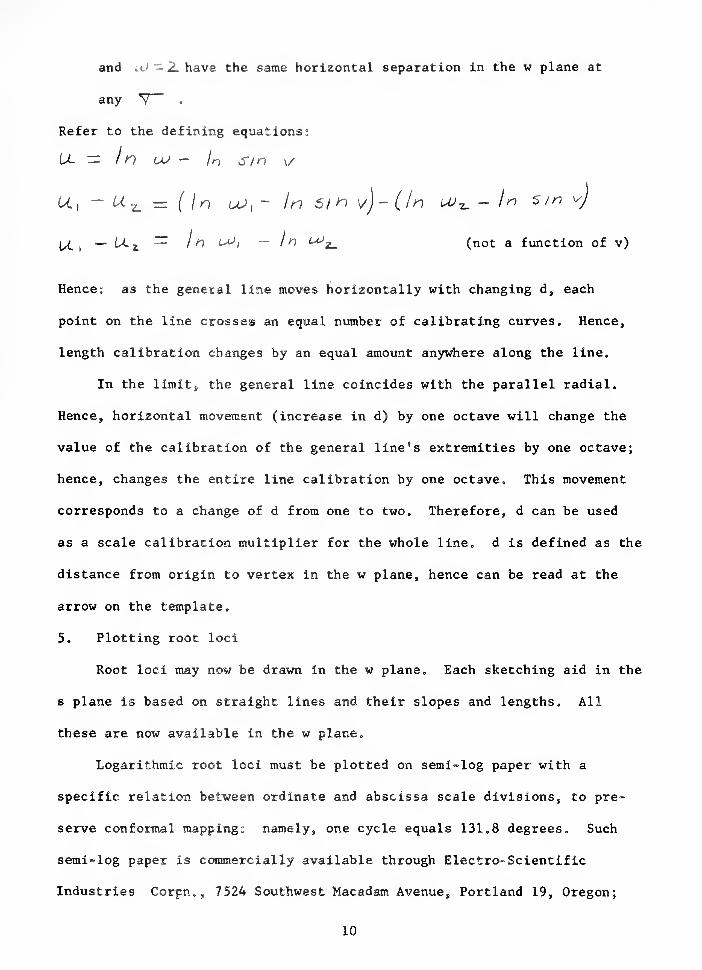
and ui - 2. have the same horizontal separation in the w plane at
any ^ .
Refer to the defining equations;
U- =: In \jj - /n s/n \/
U, - U^ --( In u>
x
~ In 51 n v)-(/n uu^- In sm »)
\Xi
— U z — In (**>t — lh ^z_ (not a function of v)
Hence: as the general line moves horizontally with changing d, each
point on the line crosses an equal number of calibrating curves. Hence,
length calibration changes by an equal amount anywhere along the line.
In the limit, the general line coincides with the parallel radial.
Hence, horizontal movement (increase in d) by one octave will change the
value of the calibration of the general line's extremities by one octave;
hence, changes the entire line calibration by one octave. This movement
corresponds to a change of d from one to two. Therefore, d can be used
as a scale calibration multiplier for the whole line, d is defined as the
distance from origin to vertex in the w plane, hence can be read at the
arrow on the template.
5. Plotting root loci
Root loci may now be drawn in the w plane. Each sketching aid in the
s plane is based on straight lines and their slopes and lengths. All
these are now available in the w plane.
Logarithmic root loci must be plotted on semi-log paper with a
specific relation between ordinate and abscissa scale divisions, to pre-
serve conformal mappings namely, one cycle equals 131.8 degrees. Such
semi-log paper is commercially available through Electro- Scientific
Industries Corpn., 7524 Southwest Macadam Avenue, Portland 19, Oregon;
10


designated as ESIAC Form 44. This paper is four-cycle, two and one-half
inches per cycle by 6.83 inches per 360 degrees, with five degree divi-
sions and 30-degree heavy divisions.
Plot root loci as follows:
a. Choose and label the four abscissa (|
ej ) decades of interest,
e.g. s .01, 0.1, 1, 10, 100.
b. Label ordinates, zero to 360 degrees.
c. Convert poles and zeros to magnitude and angle form, and plot.
(Poles and zeros jit origin can not, and need not be plotted.)
d. Sketch root locus segments on real axis (S = 0, 180 , 360 ).
(Start with pole or zero most positive and trace the real axis from
that location toward minus infinity. Those segments of the real axis
which are on the negative side of an odd number of poles (or zeros
plus poles) are root loci.) Care must be taken in this matter since
this means tracing left on the positive real axis and right on the
negative real axis. Furthermore, poles at the origin must be
counted when crossing from positive to negative real axis. When k
is negative, substitute "even" for "odd" in this rule.
e. Count poles, 1 , and count zeros, n. Then l»n root locus seg-
ments extend to infinity.
f. Locate and plot centroid of asymptotes on the real axis,
g. Angles of asymptotes are found as follows:
( z r + /) Tf(1) For positive k: Angles sz. —
;
,
(2) For negative k: Angles — &- 7T r> J r -,,, ,
li


To plot asymptotes, place template slope line coincident with graph
paper horizontal line, Q "ss required slope, slide horizontally
until template coincides with V^ and draw asymptote. Repeat until
all asymptotes are plotted.
h. Angle of emergence from a complex pole may be calculated just as
in linear theory. Keeping template slope lines horizontal, slide
template until it connects the complex pole/zero with another pole/
zero. Read slope of connecting line at template slope line and
record. Repeat for all poles and zeros. Then angle of emergence
equals 180 degrees - ^ (recorded slopes) for positive k, and 360
degrees - ^.(recorded slopes) for negative k. Place template slope
line on this calculated value, slide over to complex pole/zero, and
draw a short segment from pole or zero in template direction. This
segment is the emergence from the pole.
i. Sketch in locus. At any questionable points where accuracy is
required, use the template as a Spirule; i.e., assume a trial point;
measure angles from all poles and zeros (as is shown above) with the
template. Then, if the sum of the angles equals 180 degrees (for
positive k, or 360 degrees for negative k), the point is on the
locus. If not, another trial is needed. Direction of new trial
point is indicated by whether the sum of the angles is greater than
or less than 180 degrees.
j . Root and gain point location on the locus is analogous to linear
TTU+jmethods; i.e., k LL. 7~" of the loop transfer
// / 5 + B/function. Use template to measure distance from each pole/zero to
point on locus in question and apply above equation. (Connect two
points with template; length < (p - V-,)K where /"(=jsi as read at
12


II
APPLICATION TO SENSITIVITY DESIGN
1. Sensitivity design in the s plane
Gain and root sensitivity are important considerations in control
system design and analysis. An exact method with no approximations has
been recently developed by Rung and Thaler (2). This method uses root
locus plot in the s plane which is adaptable to the In s plane. The bal-
ance of this section is devoted to explanation of the method, defini-
tions, and adaptation to the w plane. Reference (2) contains the proofs
of the relationships between definitions to follow.
Sensitivities are defined as vector quantities.
Eq. 2.1 -- Root -Gain Sensitivity ^), ___ /, —j L
\
where q. is the root in question and L is loop gain. Thus Gain Sensi-
tivity j^ change in root position per percent change in gain. (Since
parameter changes may move the root in question in different directions,
sensitivities must be vector quantities.)
~ZT _ _2j£L- - -Si£ •
Eq. 2.2 -- Root -Zero Sensitivity J^ A yj[ j? . — frj.
Eq. 2.3 — Root -Pole Sensitivity (T '' ZZZ „JlXjL , 0/ ,
Pole and zero sensitivities H, change in root position per change in pole
or zero position. Rung and Thaler (2) also show that the sum of root and
pole sensitivities equals one.
Eq. 2.4 -- 2L > 5gr.
-f *ZL, Pj,
"~ / Using this fact alongs f r r
with equations 2.2 and 2.3, vector representations of sensitivities are
shown in Fig. 7
.
14


Fig. 7 is a root locus plot and sensitivity vector diagram of the
open loop transfer function Wt-5/ —S~(S -f l,7)(s +3)
in the s plane; k was chosen equal to 2,42, corresponding to a root atCfox
as shown.
The following construction procedure was used. Draw a vector from Q-^
toward each pole with length equal to (1/distance from ^ to pole).
These vectors define pole sensitivities, S p * Op ^)
Draw a vector from a away from each zero, defining zero sensitivities,
^ l' c^ 7T?
cf? ~c? *q} cf1
'
bz± ;~>2 ,
Form the vector sum of O^; ^ >
O^)
^>z± )~>z^
and call if U. Then 7 is the reference for length and phase of the pole
and zero sensitivity vectors $p /*•*/*«} *. j "^ * ^hase is
measured clockwise from U. For example, Sp— / lehgrh <?t ^/*> I • ,
an
Gain sensitivity gt is directionally coincident with U which is always
tangent to the root locus a (When gain changessroot must move along root
locus,) Magnitud e of the *2i vector is found from the relationship:;—I K
When the pole is chosen at the origin, ^J —^x>" ( -f if> J
In this example _ or, _. / 7 -?^ / JS7°
% = /.zzr<- *i°, S ' = #X»"- .-fc-W
_x —,.—-—™~~~?>
5:* _ (^LszSJU'**^-*-*') ~' 4f L^z**/
(measured counterclockwise as U is measured)
15

Since sensitivities are measured relative to U, the designer can
manipulate the poles and zeros of compensation devices to achieve optimum
placement of U, in addition to stability and response considerations.
This technique is demonstrated clearly by Rung and Thaler (2).
2. Sensitivity design in the In s plane
For use in the w plane, this method is most practical and rapid using
a separate graph for vector diagrams. Since straight line segments of
given length and slope can be drawn with the template, vector diagrams
can be drawn on the w plane,, but the method is slower and gains no advant-
age. After root locus and root position (or desired root position) q
have been plotted, use the template to measure and record distance and
phase angle from q to each open loop pole and zero. Then the vector
diagram can be constructed on separate linear coordinates,. The following
example problem is taken from Rung and Thaler (2), exactly, but performed
in the w plane to demonstrate the entire method.
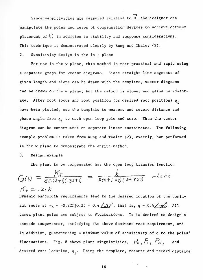
3. Design example
The plant to be compensated has the open loop transfer function
/~ /tr\ — rVf K where
Dynamic bandwidth requirements lead to the desired location of the domin-
ant roots at -q -0.2ijO.35 0.4 /l20°, that is, q = O.4/-60! All
three plant poles are subject to fluctuations. It is desired to design a
cascade compensator, satisfying the above dominant root requirement, and
in addition, guaranteeing a minimum value of sensitivity of q to the poles*
fluctuations. Fig. 8 shows plant singularities, f© li p '&. . anc*
desired root location, q 1. Using the template, measure and record distance
16

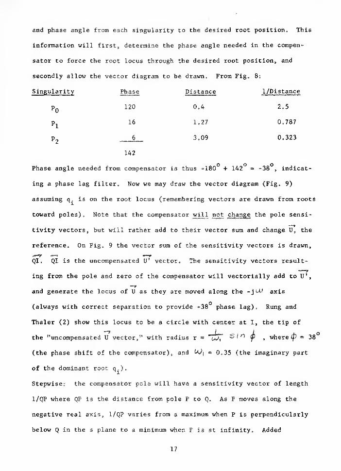
and phase angle from each singularity to the desired root position. This
information will first , determine the phase angle needed in the compen-
sator to force the root locus through the desired root position, and
secondly allow the vector diagram to be drawn. From Fig. 8:
Singularity Phase Distance 1/Distance
pQ120 0.4 2.5
px
16 1.27 0.787
P2
6 3.09 0.323
142
Phase angle needed from compensator is thus =180 + 142 = -38 , indicat-
ing a phase lag filter. Now we may draw the vector diagram (Fig. 9)
assuming q„ is on the root locus (remembering vectors are drawn from roots
toward poles) „ Note that the compensator will not change the pole sensi-
—ftivity vectors, but will rather add to their vector sum and change U, the
reference. On Fig. 9 the vector sum of the sensitivity vectors is drawn,
QI. QI is the uncompensated U' vector. The sensitivity vectors result-
ing from the pole and zero of the compensator will vectorially add to U',
—fand generate the locus of U as they are moved along the - j uU axis
o(always with correct separation to provide -38 phase lag). Rung and
Thaler (2) show this locus to be a circle with center at I, the tip of
-» / l ,(
the "uncompensated U vector," with radius r = u*>, ^> I n (p swhere (p 38
(the phase shift of the compensator)^ and ^J\ = 0.35 (the imaginary part
of the dominant root q. ).ni
Stepwise: the compensator pole will have a sensitivity vector of length
1/QP where QP is the distance from pole P to Q. As P moves along the
negative real axis, 1/QP varies from a maximum when P is perpendicularly
below Q in the s plane to a minimum when P is at infinity. Added
17


-7/ r
vectorially to U, 1/QP generates a circle of radius R = 1/2 U), 1/0.7 = 1.43,
with center vertically below I. This circle is drawn on Fig. 9 and labeled
the "M" circle. Then the sensitivity vector generated by the compensator
zero, 1/QZ, is added vectorially to the "M" circle, resulting in the U
circle, with P — UJ ,"S'i <p center at I (proof in reference two). The
U circle is drawn and labeled in Fig. 9.
In this examplesminimum pole sensitivity has been specified, hence the
longest possible U vector is desired. QU 9 the intersection of the U circle
with the extension of QI, is this vector (desired U) . Now, to find P and Z
from U, proceed as follows; Draw OJ perpendicular to QU„ Measure arcs
JN = JM =f> . Then, the direction of IN is the direction of QZ (i.e., 208°),
' —
'
oand the direction of XM is the direction of QP (i.e., 246 ). (Proof in ref-
erence two.)
Using these directions and the template , P and Z are located on the
-180° axis in Fig. 8. (P - 0.9</^180_° and Z - 0.36^180° .)
4. Summary
This method has designed the compensator to force the dominant roots to
the desired point and ensured minimum root sensitivity for cascade compensa-
tion. Furthermore, the sensitivity of each pole is known. Sensitivities
are tabulated below. -^
-CL J
18


Sensitivity design is obviously simpler in the s plane than in the
w plane. But when a root locus can not be handled in the s plane, due to
widely spread open loop poles and zeros, or when desired root location is
very near the origin, this w plane technique does work. There is no loss
in usefulness or generality caused by plotting the vector diagram on
linear coordinates. Choose the scale so that the largest sensitivity
vectors plot easily. Then any vectors which are too small to plot
accurately can be ignored, since their effect on the Uvector will be
negligible, and small sensitivities are desirable.
19


Ill
COMPENSATION DESIGN EXAMPLE
1. Compensation
This example demonstrates;
a. Clarity of w plane root locus analysis for compensator design
where a pole/zero pair is very close to the origin and other poles
and zeros are far removed
b„ Relationship of frequency and transient response to w plane root
locus.
c Breakaway-point calculation by plot of k versus real s (Wheeler
Plot) directly on root locus plot,
d. Graphical calculation of residues-
e. Direct reading scale of damping factor of dominant roots on w
plane root locus plot.
A stabilization-type servo is designed as an example by Thaler and
Brown (1). Compensation of the roll-stabilization loop in the w plane
follows:
The uncompensated open loop transfer function iss
A symmetrical compensator is chosen to meet the requirement of preserving
the gain. Trial and error methods lead to a trial compensator of
20


(o t-r.c A / -/• /)
The compensated system then has an open loop transfer function:
Fig. 10 is a root locus plot of the uncompensated system in the w
plane, showing the closed loop complex roots corresponding to k = 135,000,
and the instability of the system; the phase margin is zero. The locus
breakaway point was determined by plotting gains versus real s. This plot
can be made directly on the root locus plot, as shown.
Fig. 11 is the w plane plot of the root locus of the compensated
system, plotted over eight decades. The superiority of the w plane is
clearly demonstrated here, in its property of showing all the poles and
zeros, regardless of separation, and the complete locus.
The complex closed loop root corresponding to k = 135,000 is shown.
The phase margin is 30 degrees, and the damping factor is 0.5. Since
phase angle is a vertical coordinate in the w plane, the cosine may be
plotted as a vertical scale, to read damping factor directly.
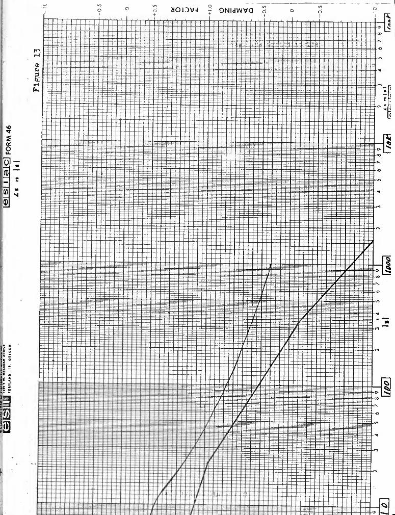
2. Frequency response
Fig. 12 and Fig. 13 show the Bode diagrams corresponding to Fig. 10
and Fig. 11srespectively. Corner frequencies occur in the same position
on the Bode diagram as the open loop poles and zeros appear in the root
locus. The frequency response can be calculated directly from the root
locus in the w plane, in a manner analogous to that in the s plane. How-
ever, the standard approximate methods are much faster and should be used,
21


unless accurate detail is required.
3. Transient response
The transient response may be calculated directly from the w plane
root locus plot by calculation of the residues.
Cu) _ Cm) iss-vct t± + -y *)U t • *. , i /)
Using roots found by Fig. 11 to factor the denominator,
CO) _ i3s-*oc( z+,sr)(s'+ g./'/J
Fes) (S+ i rr#j+z lliX3te4.Xsrt'64p't>'X*+?'<-?> /a''J
,fcs) - isFor a unit step input, f\ v 5) — ^y and
The inverse transform iss
C C 6.) - Co -t C, £ -h <=~* £ -+ ^i &
Evaluation of ^— o* C» . . • is done on the root locus plot by evaluation
of the residues. Vectors are drawn from all other roots and zeros to
root s = -2.42. Lengths and angles are recorded, and C? is evaluated
from the equation below. (The root at -0.552 is effectively cancelled by
the zero at -0.550 and could have been neglected.) This procedure is
repeated for each root and all coefficients are thus evaluated. See below;
22


t , / r* •
/ t oWs-& 4?
C, = /.**-°^L-/, <'/)(-{J_
<C? — / i" o~"£ co^^j, ^ J/ j .v tic'fj.
(-33*. <K-63'6,Ct)(riz/ /-\)(ir*-640 t 72)-0C31ZA
c<.= * CrG :<- Z—.+ /47 , yD
Cr =: 1 ; ££ £ 4-14-7,7 i
(When a root is on the real axis, the angular summation will equal ]f &TT.
or a multiple thereof. In the above calculations, angles of zero or Z Jare omitted, and angles of Jf are indicated by a negative sign in front
of the factor. Angular contributions from conjugate roots cancel, and
conjugate factors were multipled together before entering above.)
-.**** -*.«*£• -£**z£
23


IV
FACTORING A POLYNOMIAL
1. One real root, one pair of complex-conjugate roots
Any polynomial, regardless of order, may be factored by successive
applications of the root locus plot.
The following example demonstrates the factoring of a third-order case:
S* + S"£ S^-y- IC + S fz.ro
Set equal to zero and manipulate form:
5 J-f STZ S *
-f / ° * 3 i ~ GO =2 OS J
-f 5-2 5 * f / c 4 j - - ^2-^5 tf>
/
2C^ ~ ^ ^OS-i +SiS',-+/t>4f S(i '
i• - / /^J
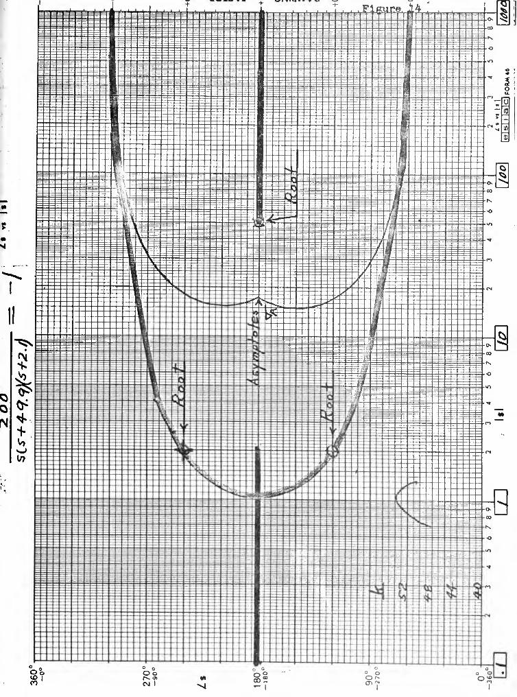
/ Z o o ~^gg _Closed loop roots of this function are factors of the original polynomial,*
(see Fig. 14). Roots were found at
s = Z £-t*o =z -/ ^fT5= Z. L-*40° - - I + -^ t/~f
by methods of Chapter I. Thus the factored form is:
2. Two pair of complex-conjugate roots
Factor 54+/^ 3f ^ 7 S Z - 2L / S ^ ZS^O
24


Set equal to zero and manipulate,
-/ =.- */g( 5-//f)Sl(S+<3+£. Z l 4?)(si- £7--2,z. l 4S~)
Closed loop roots of this function are the desired factors.
To demonstrate the principle of successive root locus plots, an
alternate manipulation will be used here in the solution of this fourth-
order case. This technique can be applied to any order.
Eq. A. — / - st+jfgi+ffyf^z/es 5(s*+W'+r7S-v<i
Now, to factor the cubic in the denominator, set it equal to zero and
manipulate as before: 2 -j- I *% S /-"jT/'J — 2/0
Closed loop roots of this function are determined by the root locus plot
in Fig. 15. These roots are:
Thus the cubic is factored: (5-/ 73)(S+?' **+f**'?zXS+% ???>***)
25

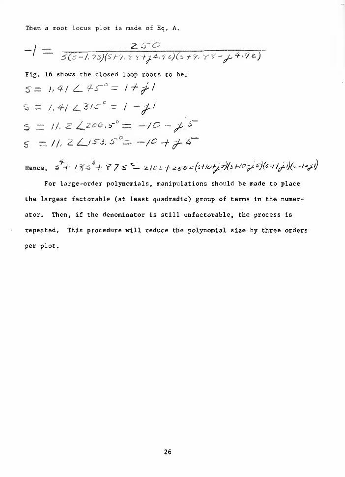
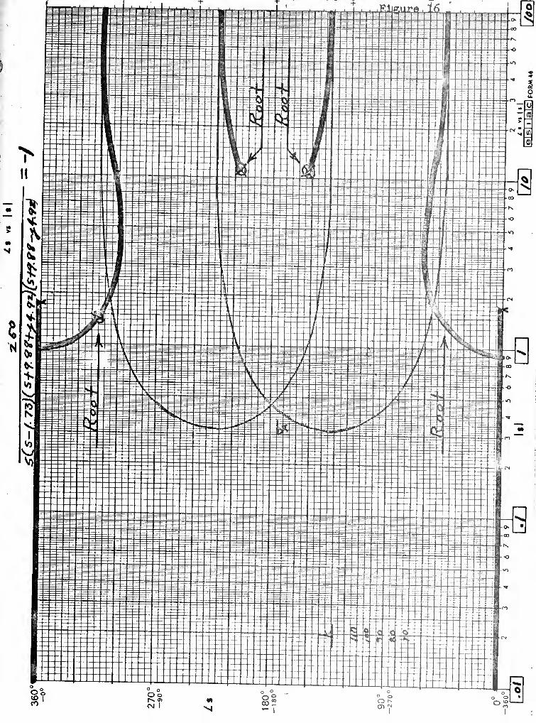
Then a root locus plot is made of Eq. A.
j ^s~o> ____Fig. 16 shows the closed loop roots to be:
S = 1,4/ ^4S-°= l+fl
s -//, z£_i^,s ^ ~/c -+^*r
Hence, 3*-/- /fS^ tf 7 S^- */Oi +*&=(^lO^)(sHO^)(s-l+f\)(^l^l)
For large-order polynomials, manipulations should be made to place
the largest factorable (at least quadradic) group of terms in the numer-
ator. Then, if the denominator is still unfactorable, the process is
repeated. This procedure will reduce the polynomial size by three orders
per plot.
26


V
CONCLUSION AND APPENDICES
1. Conclusion
Root locus plots may be sketched or constructed in the In s plane
whenever the s plane plot fails to provide satisfactory resolution of the
locus o Plotting in the In s plane is somewhat more tedious and slower
than plotting in the s plane, but does provide needed detail, while show-
ing all the poles and zeros and all of the locus of interest. The
s plane should be used in preference to the In s plane whenever it is
adequate.
This paper lists a straightforward, step-by-step procedure for
plotting in the In s plane, and includes mathematical proof of the theory,
The method is demonstrated in three practical examples in Chapters II,
III, and IV.
Root locus plots in the In s plane provide another useful tool in
the design and analysis of feedback control systems.
27


Figure 1••••(((•••••(•••••••t •••••*•••«•••»«••>! >•>••••••>•••••••••••••••••••>••>>*>•••••••-••«••••••••>••••>••••*•••• ••••••••••••••••••••••-•-••I llillilllllillll Illlllilllllllllll •«•••••••••»• ...«»••• ••••••••••• ••••l >|llltlll*lll)lllll«tl|Mllltil»l!••••••••••••>•• !•••••••••••*••••••• •••••«•••••«•••••»••••••••••••••••»*••••»••


;:!: ijjii'hn


Figure 5
h- nil iiiii 114--
'TT tt1tflllltl T 11
rrniiHiiiiiiiiiiiiiiiin lIHIlllllllTFnTTTTTffttfttftUTT
1 IIItTTT T Til ' " +? +++ E|:::|::|:fi:::Si
SHif IP til II 111 lIHffillliinn i mi i mil i il 1
1 liTTt' 1 1 1 1 1 htt ffHrffflifTtiSt
itj f fBIBIJJfljiIjllll
iUgjI 1 HirIrnl 1 m&l K|l|::i|::::::|||j |::|::||:::|;: iiijij ttliijili' it
llllllH llllllllllllllllllll 1 1 1 II 1 1 ifliT fffl -111 liii IIIII iililiiii iillrfl 111:
f-^-^iyr ft tT tff|:;-S;
||-Hj||[||j|j{Tr ii illIII uuSs 1 il1 1 j 11 I - fi-IIip1 1 if ill111Jljjl |Jljlj|J|
gggg JmmJmfflrjiU|||ftf|)|||( 1 ] jlitsp|| 4;
mi mill i ii in mill fi - -
f;
---nti wHI 1 Ml 1 T IT
lllllll
Til-TXTIts iill t+T 1 1 1 1 Iiiii; SSJ S/SSIS:
ilni llllllllllllllllllllllllllllMniiil lln SfSi1 MlSfiiwiflflrT^rl61 ijfifi8iB|
Bi SJsJs
US!
irsi 1 'flllllill
IB iiiii
ffj+wlitl/*llfira
iiiii
11 111 lllll lllll Hill IHHT11 ttir T'Tjtt Jr l'T "Hi it
liTlllillTIlilll]^^liillU^Jni 11 III --+ --J'+ff -+-T+t--r"
mmISf
Im t ! n
1Sjf
PlnF1HI ]|{|M]T|]Ttti^luttrmtl'
[ mfflm/
SjpSSTfSS:TSS
[[111
isfiipl:
I1 1
iSli'lr
MiniIIIIIIHt
Fsslsmil H itttT
ffllMiffl
MlliijIIJIIIf-
ttitgjgymjTmrx:
' I]
Ii i iiHi if T silll t
||ti jljl llil JJS TillLi111 III 1111 II
1 FsjfgL iiiiiiiimii
••gjfigsj
ffjjjff;
I--:] ufslss IjjjMif™mmm ESSS
iiiii}] in ill--wntf" {ifas
jjlllj-:
|||[||[[
:S:::3 •iff fHftffl:s|5iss ::s ffis 4: sfffPIsP +S = 4SiiftSl™
|[it hl
Fffijffi
[iiiiiiiiiif::
|flH|lfBisMil :
. 1 -H+ + --t j 1
1 |
|
i:
fff1
1
iiimii-If
'tF"-"—FTt 1 1 tl 1 TT
ifMm : wHi
fY"-~-S'j tt.
:: fflHffii ::±±±ffi :±± |::|i S- g||:
1ShSS : iiiiiiiiiiifSi -OTIT44T—TT -i-STStSr PtFftj-'pliTpl^S|5-"fiiB ES
TT : "m'H t
'
II1 1 M tl ITT L ±ffftft ijjp JjjtjL
iiimii ilii''!!! Ttlftrsfss
--t-|--^:S :{
: ffiSi
' llllllI
- 1J
:: fit88 l||ff "jnnnj: :B:::3
"
" T T 1 nTTT TTIlls1
:;g|g:::fi|:#|::i
""111 Villi' T"TTT 1 1 !|f TtTf
::$fi|fi$^S|
HtHtmm px 11 ::fj ::
mm
:
:g:-3:-|M1|hb|1 ::||J:BB§::3II±J:KE:::|BgB
t-WHLlilliill
i T 1 111 wt-swiiii :
llrf:
i
l I T Mm + :"Tit"St lit' T"T""
r^1—
T
::::M|s^t^LJjjJj 1 1 Iff] j j
ifffff J
""lllll HtTTTTTTTTTi """-::::
||D-||::1:1|niiniiiii II l|l llll nxx ux i—
eexI


Figure 6
t 1
V)
.<0Si
ft
0)
.ft-4
v/i
o *?oto <V.
33


?????•????•??? ???•??•" '•"!•!!•!••••••!!•!•!•*!••••-•*•••«•«••••••••.•••••••••••••••••••«•••••:HE:::H:HH::HHH:HH:HHH:H:H!:::::H:::::::::::i::::
Figure 7•••••••••••••••••••a* •!•••••• •••••••••••••••••• •••••••• •••••••••••••• .••••••• ••)«• •••••••••••••••••••• ••• •••• ••••


OoCO
o oLSL


Figure 9


2 2 o o aoiDVd S ONidwva 2 © 2 °• it. L1A con d *. o ! IB J
' ' ' '?- "j 11 .'
I'
| ' I l' 1 S 1 'l I 'l 1 1 1 1 1 \
||
!'
f{' ( 'il i'
' '
't ('
i' V ;' \J"
J '
i J L_l_ 1-*1
i_ : _l_ _L_ (---00
L ___f - - . -L - X- ^T i"~l T-j : 1~i~ ; \.T j
T-% H(
! ' 4 E==:-I
: *HxItlT"^ r ±±±f .
• _i_ j—_—H+i—!-:£=-- -
:
i ±T±i _t "
; i-
;-f- t-— = i—r i "tf ~ -- ---..--", [
U !f f " "_-:-- ..:.-
r "'' t~ ~T T
. "J" - o
|—-|---^ --^""----^-"-i
f 4- -- r ~ "N
3
H1
. _
3I '
— ~ " ~_—:34j
—~ — — ~y~ ~r}~ :
~~*~ *
==========; ======================: --.---:-; -..-. i_- . ------
= — — — ——— — = = — -— — — — — —— — — — — — — = — — = = — = = — -} -:_:--— ^ — = = ==: = = = = =r j: = = = = =; = == = =
= — E = E — — — . ============ =
—
=E=E--— = ~- 4 _______—p—--
—
:-— 1
—
----^---p-*3
-E — — — ~ — — — ~ —
-
:—— — — —— — — — — — — —- .— — — ——— — — — — — .«»
= := = ==== = = ==] ~- = =——==—= = =—— ==E:EE==E= = =z — t — _ __
— ~^|~^ —~ ~ = = =3 —— ~~~~ ~ —~~ = = = = = =: = = = = = = = : T = == ==p: == == ==== = = === = === == = === = = = = =
llllllllllli linn ii ilii ii ii ii ii iii!
CNk
Z it
t= —^=~ — — — — — — — W^ — — 1=3=: — — — — — = — r=^^:==i==^=:==r:: N=====-=--=== fe = = --5j --:.-_|4.- - =ri; = ~
1: = = ; --00
«
= = = = E"= = = = = =il*EE"^ = = E = E:E IEEE== = S = EEISS=: = = SSE = ^^ = = — — -Mi- =.=.=.=.=.=.=.=.=.=.=:=..?>.
::C:=*» === = = = === = = fc
1=1= 11 !====!ifci^ 1=1=11 IIS 11 11 11 11~jy = «l ____.__^p____— —— ——-—-_ -m
^P= fyA ;= = == ==== ii =l I
?* " g 4!l^^^^;4!^^4z;^^^ ^. — — JH__ _ _^ = = ^^._^^^^^= .-<t
llllllllllli =1ȤIe llllllllllli II Ilii!
EE== ============== =|3== ====== ======
1— ^:^^>--ZI---^-----^ £lE^^-^ZZZI-^ZiZ--l -cn
i_ M c-
1
llllllllllli III! I |jl| || lllllliillllHIrE^E^E^E^E^EEEEE^BE^EEE^EE^EEEEEEEEE-"
%
llllllllllllliilll|l|=llllil^llllll;
================^E=======^======== =5 -<o
= = = = = = ;^— — — ^ = = = jfi_ ^p — — — — — — —— — — — — — — — — — —.r^
•• Hfl^^^^ffltillllllllllMffffPMi
, i% \
r m - ! ^i^ -/- i,
^l . AW t _tc
= = = — "" -- n ^Itr-Il ~ — iltf^E <•» m~~^~^^ = = = = ^==iEE=i === = ' | ^^Sfl


±±±±±d ^bj ::_>______ ______±_:±_____- *l ^ita, LmW- -t XX X » -\ NBftg fT Z t X XXX --i -: r ... +X
-o*
-OLL
rI/. ; x 1 --I 1 1— --o
' H--' i
"
~*~
\ i» ^l__ L f:---- ±-' _j_
1 #1^ II -§_. X - X^ ^" it -
_. S. t f -»y\Jl v
- J*-P ]b. - ' ---{ l-
"
:
'-.l
- ir - v ^___s____lp______^^^ •
u
I
ML m IB
Jfl
- mf -j v- - m -f.!D-: K - 1—- - - .... _ H . _.._.. -—
" iR— B --- ---•£ -_-__— _:_
_:
* . _|_ = _ = 3 5X----=--3iisiiB|iiiiiiifliiiiiiiii=illllll=l*Xr T S TTTl'MIJ 4 1 1 IBM 1 111 fl 1 1» 1 1111 1 1 111
>::-^i -: ; ?=r ^ -\ :- ,k ii :. -._
_ _ — _ -l mm —
ffil 1 11 mm m TiTfiI 1 1 ITTTIil mT_____________ _|
|B ____________________ f»>
v., :
B:
fB CN
> _fS J-•J —^Vo n M
•*£^ m~5i
~ _ Y= = = = = = = = = = = = =ag=== = = = = = = = = = = = = = = = = = = -co
—————-——=— —^JB— — — ———————————————— ————••o
"5
V/J
f---- ~ = - = = ii -- = - = = = = = = - = -- = = - = - = = = = =" ,0
»K__ = =|iii =___ = = = = EE = = = = = = = = = = = = = = l = = = •
pi= — ?£»? —EEEEEEEEEEEEEEEEEEEEEEEEEEEEE-*">
~"
^EEEEEEEEEEEEEEEEEEE^EE^^E E. CM
\
II 11 1 1 n
II
l!> I VSJ*
=1=1111111111=111111111111111=11111 till 11 1111 II 111111 1111111111111=1="
»
= = = = = == := === e = = ~==.=- = e|==
;
= =. = :h43|------------- = s ==^-g:-g- Jl-:--;-^-
=--^"'°= =^=^=^=== ===^ =^^==== = ==^^ = ~=e=^ = ^£t-: 1 E____=____=e_: i.^=p EEEl^ Lr-EEEEEEEEEE:_:EEEEEEEE:_;EEEEEr-:~_~I:j 8:= EE= ^ = EE:= = =: = = EEE=: = = == =— = - == =— == —— —— —
p
>
, ,—__ — —.jQ - -,
f. —i_:
____: -— -. ---— --__:-- 1" i|-._-______._^__________._._..._._r
a. ^m
y - ... _l_ . 1 <
t o o o O 5m ^ ° "Cl^
CO
Oocvi I
00_o
Of-


aoiDVd oNidwva 2
o
O


u '

J_L
OotO
|
CO
° oOo<V4 I
£
o2oo2
o oOf» o o
O *I


BIBLIOGRAPHY
1. Thaler, G. Jo and R. G. Brown. Analysis and Design of FeedbackControl Systems. McGraw-Hill, 1960.
2. Rung, B. T. and G. J. Thaler. Feedback Control Systems: Design withRegard to Sensitivity. U. S. Naval Postgraduate School ResearchReport No. 41. 1964.
46