ABHELSINKI UNIVERSITY OF TECHNOLOGYDepartment of Electrical and Communications Engineering
MEASUREMENTS FOR MODELLING OF WIDEBAND
NONLINEAR POWER AMPLIFIERS FOR WIRELESS
COMMUNICATIONS
Gilda Gabriela Gamez Gonzalez
Master’s Thesis that has been submitted for official examination for the degree of
Master of Science in Espoo, Finland on September 27th, 2004.
Supervisor Professor Timo Laakso
Instructor M.Sc. Viktor Nassi
HELSINKI UNIVERSITY OF TECHNOLOGY Abstract of the Master’s Thesis
Author: Gilda Gabriela Gamez Gonzalez
Title of the Thesis: Measurements for modelling of wideband
nonlinear power amplifiers for wireless
communications
Date: September 27th, 2004 Pages: 117
Department: Department of Electrical and Communications
Engineering
Professorship: Signal Processing
Supervisor: Professor Timo Laakso
Instructor: Viktor Nassi
Power amplifier linearity is an important topic in today’s communication
systems, especially in wireless communications where amplifier distortion
affects transmissions not only in the used channel but in adjacent ones.
Generally, a power amplifier is more efficient when it is operated at high power
levels. However, this results in distortion of the output signal. Therefore,
highly linear power amplifiers are required for efficient wireless communications.
The objective of this thesis is to provide the basis for performing accurate mea-
surements of power amplifiers in order to obtain enough reliable data helpful to
model their nonlinearity. The objective was achieved by performing practical
measurements with different types of signals from which diverse modelling
parameters were obtained. Single- and two-tone signals were used to test the
amplifier. In addition, a multisine signal, example of high peak-to-average
ratio signal, was chosen to perform multi-tone signal measurements.
It was demonstrated how the frequency-dependent and frequency-independent
behavior of the amplifier can be accurately modelled based on the single-tone
signal measurements performed in this thesis. Furthermore, the exactness of
the measurements was analyzed and it was determined that highly accurate
measurements are a complicated process that involves numerous factors.
Moreover, it was shown that amplifier measurements have a very wide usa-
bility. Mainly, the contribution of this thesis is represented by a full set of
measurement results that can be used for future modelling of amplifiers.
Keywords: Amplifier, nonlinearity, measurement, network analyzer, spectrum
analyzer, modelling parameter, two-tone signal, multisine signal.
i
TEKNILLINEN KORKEAKOULU Diplomityon tiivistelma
Tekija: Gilda Gabriela Gamez Gonzalez
Tyon nimi: Laajakaistaisten epalineaaristen tehovahvistimien
mittaaminen matkaviestinjarjestelmissa
mallintamista varten
Paivamaara: 27. syyskuuta 2004 Sivumaara: 117
Osasto: Sahko- ja tietoliikennetekniikan osasto
Professuuri: Signaalinkasittelytekniikka
Tyon valvoja: Professori Timo Laakso
Tyon ohjaaja: Viktor Nassi
Tehovahvistimen lineaarisuus on tarkea aihe nykyajan tietoliiken-
nejarjestelmissa. Erityisen tarkeaa se on matkaviestinjarjestelmissa, joissa
vahvistimen epalineaarisuus vaikuttaa tiedonsiirtoon lahetyskanavan lisaksi
myos viereisissa kanavissa. Yleisesti tehovahvistimen hyotysuhde on parempi,
kun sita kaytetaan korkealla teholla. Tama kuitenkin aiheuttaa vaaristymaa
lahtosignaaliin.
Taman diplomityon tavoitteena on luoda perusta tarkkojen tehovahvistinmit-
tausten suorittamiseen, joita voidaan kayttaa tehovahvistimien mallintamiseen.
Tavoite saavutettiin suorittamalla mittauksia erityyppisilla signaaleilla,
joista saatiin erilaisia mallinnusparametreja. Yksi- ja kaksitaajuussignaa-
leja kaytettiin vahvistimien testaamiseen. Lisaksi monitaajuusmittauksissa
kaytettiin monisinisignaalia, joka on esimerkki signaalista jolla on korkea
huippu- ja keskiarvotehon suhde.
Tyossa osoitettiin, kuinka vahvistimen taajuusriippuva ja taajuusriippu-
maton kayttaytyminen voidaan tarkasti mallintaa suoritettujen mittausten
avulla. Mittausten tarkkuus analysoitiin ja sen pohjalta todettiin, etta
erittain tarkkojen mittausten tekeminen on monimutkainen prosessi, johon
lukuisat tekijat vaikuttavat. Lisaksi osoitettiin etta vahvistinmittauksilla on
erittain laaja kaytettavyys. Tyon tulokset on esitetty taydellisten mittaus-
tulosten muodossa, joita voidaan jatkossa kayttaa vahvistimien mallintamiseen.
Avainsanat: Vahvistin, epalineaarisuus, mittaus, piirianalysaattori, spektria-
nalysaattori, mallinnusparametri, kaksiaanisignaali, monisinisignaali.
ii

UNIVERSIDAD TECNOLOGICA DE HELSINKI Resumen de la Tesis de Maestrıa
Autor: Gilda Gabriela Gamez Gonzalez
Tıtulo de la Tesis: Mediciones para el modelado de amplificadores
de potencia no lineales de banda ancha para
comunicaciones inalambricas
Fecha: 27 de septiembre de 2004 Paginas: 117
Departamento: Departamento de Ingenierıa Electrica y
Comunicaciones
Profesorado: Procesamiento de Senales
Supervisor: Profesor Timo Laakso
Instructor: Viktor Nassi
La linealidad de amplificadores de potencia es muy importante en los sistemas
de comunicacion actuales, especialmente en comunicaciones inalambricas donde
la distorsion de los amplificadores afecta las transmisiones tanto en el canal en
uso como en canales adyacentes. En general, un amplificador es mas eficiente
cuando es operado a altos niveles de potencia. No obstante, esto produce
distorsion en la senal de salida. Por lo tanto, amplificadores de potencia
altamente lineales son requeridos para comunicaciones inalambricas eficientes.
El objetivo de esta tesis es proporcionar las bases para realizar medidas
precisas de amplificadores de potencia que den como resultado informacion
util para su modelado. Este objetivo fue alcanzado mediante mediciones
utilizando diferentes tipos de senales de las cuales se obtuvieron diversos
parametros. Senales de uno y dos tonos fueron usadas para probar el ampli-
ficador. Asimismo, una senal multi-seno, ejemplo de senales con alta relacion
pico a promedio, fue seleccionada para realizar mediciones de senales multi-tono.
Fue demostrado como el comportamiento dependiente e independiente de
frecuencia del amplificador puede ser correctamente modelado en base a
las mediciones de senal de un tono realizadas en esta tesis. Asimismo, se
analizo la exactitud de los resultados y se determino que las mediciones de
alta precision son procesos complicados que involucran numerosos factores y
que las mediciones de amplificadores tienen un amplio campo de aplicacion.
La aportacion principal de esta tesis es la serie de resultados obtenidos que
pueden ser utilizados para modelar amplificadores de potencia.
Palabras clave: Amplificador, no-linearidad, medicion, analizador de red, ana-
lizador de espectro, dato para modelado, senal de dos tonos, senal multi-seno.
iii

Acknowledgement
To my grandfather, Rafael, for his million advices. To my mother, Gilda, (no
words to express my love and gratitude). To my father, Jorge, for his continuous
support. To Ina for make me feel that there are people missing and loving me back
in my country. To the Gonzalez-Martınez and Gonzalez-Moreno families. And,
over all, deeply to my late grandmother, Eve(†), who educated and made of all of
us a honest and united family.
To my academic father, Prof. Timo Laakso, for supervising and guiding my thesis
and to my technical instructor, Viktor Nassi, for his always willing and useful help.
To Prof. Pertti Vainikainen and Prof. Sven-Gustav Haggman for facilitating the
cooperation with the Communications and Radio Communications Laboratories
and to Viktor Sibakov, Rauno Kytonen, Jarmo Kivinen and Viatcheslav “Slava”
Golikov for their advice in the practical part of the thesis.
To Peter Jantunen, because of his patience, personal support and for checking
my whole thesis. To Mei Yen Cheong, for her friendship, advice and support on
my working time, to Edgar Ramos for being my friend and helping me with the
spanish translations and to Stefan Werner for his comments on this research.
To the planning officer Anita Bisi for listening patiently all my concerns during
my master’s studies. To the nice secretaries Anne, Mirja and Marja, for always
assisting me with a smile.
To Katri, Niko, Heikki and their families, for making my time in Finland nice,
comfortable and for teaching me to understand Finnish people’s behavior. To my
friends in Finland Enrique, Carmen and Karina for giving me a sense of family in
this country. To Nadia for her friendship and continuous advices on my personal
life. To all my Mexican and foreign friends who give color to my life and to my
working mates for making the long (and short) working days easy-going.
THANK YOU.
iv

Agradecimientos
A mi abuelito, Rafael, por sus millones de consejos. A mi mama, Gilda, (no hay
palabras para expresar mi carino y gratitud). A a mi papa, Jorge, por su apoyo de
siempre. A Ina por hacerme sentir que hay personas que me extranan y quieren
en mi paıs. A las familias Gonzalez-Martınez y Gonzalez-Moreno. Y, sobre todo,
profundamente a mi abuelita Eve(†), quien nos educo e hizo de todos nosotros una
familia honesta y unida.
A mi padre academico, Prof. Timo Laakso, por supervisar y guiar mi tesis y a mi
instructor tecnico, Viktor Nassi, por su siempre dispuesta y util ayuda. A los pro-
fesores Pertti Vainikainen y Sven-Gustav Haggman por facilitar la cooperacion con
los laboratorios de Comunicaciones y Radio Comunicaciones y a Viktor Sibakov,
Rauno Kytonen, Jarmo Kivinen y Viatcheslav “Slava” Golikov por sus consejos
en la parte practica de esta tesis.
A Peter Jantunen, por su paciencia, apoyo personal y por revisar mi trabajo du-
rante todo el proceso. A Mei Yen Cheong, por su amistad, consejos y apoyo en mi
tiempo de trabajo, a Edgar Ramos por ser mi amigo y ayudarme con las traduc-
ciones a espanol y a Stefan Werner por sus comentarios en esta investigacion.
A la coordinadora Anita Bisi, por escuchar pacientemente todas mis preocupa-
ciones durante mis estudios de maestrıa. A las simpaticas secretarias Anne, Mirja
y Marja por siempre ayudarme con una sonrisa.
A Katri, Niko, Heikki y sus familias, por hacer mi tiempo en Finlandia agradable,
comodo y por ensenarme a entender el comportamiento de la gente finlandesa. A
mis amigos en Finlandia: Enrique, Carmen y Karina por darme el sentimiento de
una familia en este paıs. A Nadia, por su amistad y continuos consejos en mi vida
personal. A todos mis amigos mexicanos y extranjeros que dan color a mi vida y
a mis colegas por hacer llevaderos los largos (y cortos) dıas de trabajo.
GRACIAS.
v
Contents
Abstract i
Acknowledgement iv
Agradecimientos v
List of Acronyms x
List of Symbols xiii
List of Figures xvi
List of Tables xix
1 Introduction 1
1.1 Motivation . . . . . . . . . . . . . . . . . . . . . . . . . . . . . . . 1
1.2 Objective . . . . . . . . . . . . . . . . . . . . . . . . . . . . . . . 2
1.3 Outline of the thesis . . . . . . . . . . . . . . . . . . . . . . . . . 3
2 Amplifiers 5
2.1 Power amplifiers . . . . . . . . . . . . . . . . . . . . . . . . . . . . 6
2.2 Classes of amplifiers . . . . . . . . . . . . . . . . . . . . . . . . . 11
2.3 Linearity and distortion . . . . . . . . . . . . . . . . . . . . . . . 15
2.4 Distortion in power amplifiers . . . . . . . . . . . . . . . . . . . . 16
2.5 Summary of the chapter . . . . . . . . . . . . . . . . . . . . . . . 18
vi

3 Power amplifier distortion measures 19
3.1 Distortion measures using single-tone signals . . . . . . . . . . . . 20
3.1.1 Second harmonic distortion . . . . . . . . . . . . . . . . . 20
3.1.2 Third harmonic distortion . . . . . . . . . . . . . . . . . . 22
3.1.3 Higher-order harmonic distortion . . . . . . . . . . . . . . 24
3.1.4 1 dB compression point and back-off parameter . . . . . . 26
3.1.5 AM-AM and AM-PM characteristics . . . . . . . . . . . . 27
3.1.6 Frequency sweep . . . . . . . . . . . . . . . . . . . . . . . 28
3.2 Distortion measures using two-tone signals . . . . . . . . . . . . . 29
3.2.1 Intermodulation products . . . . . . . . . . . . . . . . . . 30
3.2.2 Intermodulation distortion ratio (PIMR) . . . . . . . . . . 32
3.2.3 IMD and Carrier-to-Noise Ratio (CNR) . . . . . . . . . . . 33
3.2.4 Spurious signals . . . . . . . . . . . . . . . . . . . . . . . . 33
3.3 Distortion measures using multi-tone signals . . . . . . . . . . . . 34
3.3.1 Adjacent Channel Power Ratio (ACPR) . . . . . . . . . . 36
3.3.2 Multi-tone Intermodulation Ratio (MIMR) . . . . . . . . . 36
3.3.3 Noise Power Ratio (NPR) . . . . . . . . . . . . . . . . . . 37
3.3.4 Phase distortion . . . . . . . . . . . . . . . . . . . . . . . . 37
3.4 Summary of the chapter . . . . . . . . . . . . . . . . . . . . . . . 39
4 Background for planning measurements 40
4.1 Methods for modelling power amplifiers . . . . . . . . . . . . . . . 41
4.2 Parameter estimation theory . . . . . . . . . . . . . . . . . . . . . 43
4.3 Summary of the chapter . . . . . . . . . . . . . . . . . . . . . . . 45
5 Power amplifier measurement planning 46
5.1 Before measurements . . . . . . . . . . . . . . . . . . . . . . . . . 47
5.1.1 Choice of input signal . . . . . . . . . . . . . . . . . . . . 48
5.1.2 Equipment . . . . . . . . . . . . . . . . . . . . . . . . . . . 49
5.1.3 Calibration . . . . . . . . . . . . . . . . . . . . . . . . . . 54
5.1.4 Noise . . . . . . . . . . . . . . . . . . . . . . . . . . . . . . 55
vii
5.2 Performing measurements . . . . . . . . . . . . . . . . . . . . . . 58
5.2.1 Passive device measurements . . . . . . . . . . . . . . . . . 58
5.2.2 Single-tone signal measurements . . . . . . . . . . . . . . . 61
5.2.3 Two-tone signal measurements . . . . . . . . . . . . . . . . 63
5.2.4 Multi-tone signal measurements . . . . . . . . . . . . . . . 67
5.3 Summary of the chapter . . . . . . . . . . . . . . . . . . . . . . . 70
6 Power amplifier measurement results 71
6.1 Passive device measurements . . . . . . . . . . . . . . . . . . . . . 72
6.1.1 Devices needed to interconnect measuring systems . . . . . 72
6.1.2 Devices needed to perform correct measurements . . . . . 76
6.2 Single-tone signal measurements . . . . . . . . . . . . . . . . . . . 78
6.2.1 Results obtained using a network analyzer . . . . . . . . . 78
6.2.2 Results obtained using a spectrum analyzer . . . . . . . . 85
6.3 Two-tone signal measurements . . . . . . . . . . . . . . . . . . . . 88
6.3.1 Generated two-tone signal . . . . . . . . . . . . . . . . . . 88
6.3.2 Two-tone signal applied to amplifier . . . . . . . . . . . . 89
6.4 Multi-tone signal measurements . . . . . . . . . . . . . . . . . . . 92
6.4.1 Generated multisine signal . . . . . . . . . . . . . . . . . . 92
6.4.2 Multisine signal applied to amplifier . . . . . . . . . . . . . 94
6.5 Summary of the chapter . . . . . . . . . . . . . . . . . . . . . . . 97
7 Measurement errors and use of results 99
7.1 Discussion of measurement errors . . . . . . . . . . . . . . . . . . 100
7.2 Using the measurement results . . . . . . . . . . . . . . . . . . . . 102
7.3 Summary of the chapter . . . . . . . . . . . . . . . . . . . . . . . 104
8 Conclusions and future work 105
References 108
viii

Appendices
A Summary of equipment specifications I
B Setup systems to perform measurements VI
C Processes to perform measurements XII
D Data and plots of measurement results XIX
ix

List of Acronyms
µs microsecond
3G Third-generation (cell-phone technology)
AC Alternating Current
ACPR Adjacent Channel Power Ratio
AM-AM Amplitude Modulation to Amplitude Modulation
AM-PM Amplitude Modulation to Phase Modulation
APC Amphenol Precision Connector
APC-2.4 2.4 mm Amphenol Precision Connector
APC-3.5 3.5 mm Amphenol Precision Connector
Att. Attenuation
AWG Arbitrary Waveform Generator
BW Bandwidth
C Celsius / Centigrade
CIR Carrier-to-Interference Ratio
cm. centimeter
CNR Carrier-to-Noise Ratio
CP Compression Point
DANL Displayed Average Noise Level
dB decibel
dBc decibel (referenced to the carrier power)
dBm decibel (referenced to one milliwatt)
DC Direct Current
deg degree
DUT Device Under Test
e.g. exempli gratia (Latin: for example)
EER Envelope Elimination and Restoration
EIKA Extended Interaction Klystron Amplifier
x
etc. et cetera (Latin: and so forth)
et al. et alii / et alia (Latin: and others)
FDM Frequency Division Multiplexing
FET Field Effect Transistor
FIR Finite Impulse Response
GaN Gallium Arsenide
GHz Giga Hertz
HMM Harmonic Mixing Mode
Hz Hertz
i.e. id est (Latin: that is)
I/Q In-phase / Quadrature
IBO Back-off referred to input level
IF Intermediate Frequency
IFFT Inverse Fast Fourier Transform
IM Intermodulation
IMD Intermodulation Distortion
IMP Intermodulation Product
IMP3 Third Intermodulation Product
in. inch
IP Intercept Point
J Joule
K Kelvin
kHz kilohertz
kW kilowatt
LINC Linear Amplification using Nonlinear Components
LSE Least Squares Estimator
max. maximum
MHz MegaHertz
MIMR Multi-tone Intermodulation Ratio
MS MegaSample
MSK Minimum Shift Keying
mW milliwatt
mV millivolt
NLWM Nonlinearity With Memory
NPR Noise Power Ratio
xi
ns nanosecond
NWA Network Analyzer
OBO Back-off referred to output level
OFDM Orthogonal Frequency Division Multiplexing
PA Power Amplifier
PAR Peak-to-Average Ratio
PDF Probability Density Function
PHEMT Pseudomorphic High Electron Mobility Transistor
ppm parts per million
PSK Phase Shift Keying
PWM Pulse-Width Modulation
QAM Quadrature Amplitude Modulation
QBL Quasi-band-limited Pulses
QPSK Quaternary Phase Shift Keying
RF Radio Frequency
rms root-mean-square
SA Spectrum Analyzer
sec. second
SG Signal Generator
SMA Sub-Miniature A
SNR Signal-to-Noise Ratio
S-parameter Scattering parameter
SR Sampling Rate
SSPA Solid State Power Amplifier
SWR Standing Wave Ratio
T Temperature
THRU Through (from Through Response Calibration)
TRW Travelling Wave Resonator
TWT Travelling Wave Tube
TWTA Travelling Wave Tube Amplifier
W Watt
V Volt
VSG Vector Signal Generator
WLSE Weighted Least Squares Estimator
ZMNL Zero-Memory Nonlinearity
xii

List of Symbols
α Complex constant
η Power efficiency
ξ Unknown parameter
π Pi (≈ 3.1416)
τ Time delay
τs Operating noise figure / Noise sensitivity
φ Phase shift
ωC Angular frequency of the carrier signal
ωM Angular frequency of the modulating signal
ω Angular frequency
Φ Phase
Ω Ohm
Degree
1 dB CP One dB Compression Point
2Tonemax.sep. Two tones maximum separation
A Amplitude
AM Amplitude of the modulating signal
B Bandwidth of a system
CID Difference between the CIR and the intrinsic CNR
CNRI CNR caused by the system noise
CNRN&IMD CNR including noise and IMD effects
d[R] R-data point
D R-points data set
f Frequency
f Fundamental frequency
F Noise factor
f0 Center frequency
xiii

fb Basic frequency
fc Carrier frequency
fIMP Frequency of the intermodulation product
fm Frequency of a baseband signal
foff Offset frequency
g A function
IN Input
IP2 Second order Intercept Point
IP3 Third order Intercept Point
k Constant factor
K Power gain
Kφ Phase shift constant
m Positive integer (excluding zero)
M(t) Modulating signal
Ms(t) Multisine signal
MaxIMP Maximum Intermodulation Product
n Positive integer (excluding zero)
N Order of the nonlinearity
Nf Noise figure
OBO1dBCP Back-off referred to output level and 1 dB CP
OBOsat Back-off referred output level and saturation level
OUT Output
p(ξ) Prior PDF (summarizing ξ knowledge before any data is
observed)
p(D | ξ) Conditional PDF (summarizing a priori knowledge of D
conditioned on knowing ξ)
p(D; ξ) Probability density function of D, which depends on ξ
p-p Peak-to-peak
P Power
PB Bandwidth power
PIMR Intermodulation Distortion Ratio
PIN Input power
PIN,avg Average input signal power
PIP3 Power of the third-order intercept point
xiv
Pn Noise power
POUT Output power
POUT,A1 Output power in one input tone
POUT,avg Average output signal power
POUT,max Maximum output power
rn Noise ratio
R Positive integer (excluding zero)
S Scattering parameter
sat. saturation level
SNRinput Input Signal-to-Noise Ratio
SNRoutput Output Signal-to-Noise Ratio
t Time
T Absolute temperature
Ta Actual temperature
Te Effective input noise temperature
Tn Noise temperature
To Operating temperature
Vcc Voltage at the common collector
Vdc Direct current voltage
x(t) Input signal
y(t) Output signal
Z Boltzmann constant (≈ 1.38 × 10⁻²³ J/K)
xv

List of Figures
1.1 Organization of the thesis 4
2.1 Basic TWTA 6
2.2 Basic SSPA (Class A configuration) 7
2.3 Example of TWTA and SSPA transfer curves 8
2.4 Class A amplifier’s operation point 12
2.5 Class B amplifier’s operation point 12
2.6 Class AB amplifier’s operation point 13
2.7 Transfer characteristics of ideal and nonlinear amplifier 17
3.1 Example of second harmonic distortion 21
3.2 Second order intercept point of an amplifier 21
3.3 Example of third harmonic distortion 22
3.4 Third order intercept point of an amplifier 23
3.5 Even-order harmonic components of nonlinear amplifier 24
3.6 Odd-order harmonic components of nonlinear amplifier 25
3.7 1 dB compression point and back-off parameter 26
3.8 AM-AM and AM-PM transfer characteristics of amplifier 28
3.9 Frequency sweep of amplifier transfer characteristic 29
3.10 Illustration of a two-tone signal 30
3.11 Ninth-order in-band distortion with a two-tone input signal 31
3.12 Seventh-order nonlinearity with a two-tone input signal 32
3.13 Orthogonal frequency division multiplexing 34
3.14 Adjacent channel power ratio 36
3.15 Multi-tone intermodulation ratio 36
3.16 Noise power ratio 37
3.17 Phase distortion in time domain 38
4.1 Commonly used modelling methods 42
4.2 Commonly used estimators 44
xvi
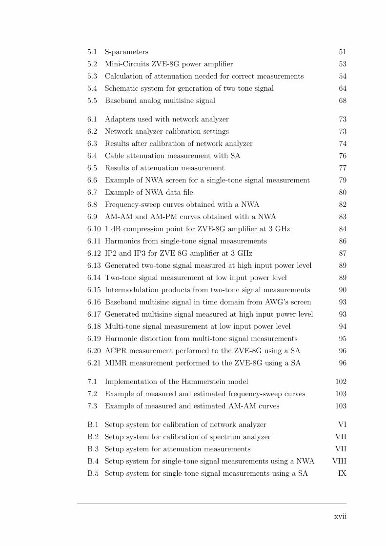
5.1 S-parameters 51
5.2 Mini-Circuits ZVE-8G power amplifier 53
5.3 Calculation of attenuation needed for correct measurements 54
5.4 Schematic system for generation of two-tone signal 64
5.5 Baseband analog multisine signal 68
6.1 Adapters used with network analyzer 73
6.2 Network analyzer calibration settings 73
6.3 Results after calibration of network analyzer 74
6.4 Cable attenuation measurement with SA 76
6.5 Results of attenuation measurement 77
6.6 Example of NWA screen for a single-tone signal measurement 79
6.7 Example of NWA data file 80
6.8 Frequency-sweep curves obtained with a NWA 82
6.9 AM-AM and AM-PM curves obtained with a NWA 83
6.10 1 dB compression point for ZVE-8G amplifier at 3 GHz 84
6.11 Harmonics from single-tone signal measurements 86
6.12 IP2 and IP3 for ZVE-8G amplifier at 3 GHz 87
6.13 Generated two-tone signal measured at high input power level 89
6.14 Two-tone signal measurement at low input power level 89
6.15 Intermodulation products from two-tone signal measurements 90
6.16 Baseband multisine signal in time domain from AWG’s screen 93
6.17 Generated multisine signal measured at high input power level 93
6.18 Multi-tone signal measurement at low input power level 94
6.19 Harmonic distortion from multi-tone signal measurements 95
6.20 ACPR measurement performed to the ZVE-8G using a SA 96
6.21 MIMR measurement performed to the ZVE-8G using a SA 96
7.1 Implementation of the Hammerstein model 102
7.2 Example of measured and estimated frequency-sweep curves 103
7.3 Example of measured and estimated AM-AM curves 103
B.1 Setup system for calibration of network analyzer VI
B.2 Setup system for calibration of spectrum analyzer VII
B.3 Setup system for attenuation measurements VII
B.4 Setup system for single-tone signal measurements using a NWA VIII
B.5 Setup system for single-tone signal measurements using a SA IX
xvii

B.6 Setup system for two-tone signal measurements X
B.7 Setup system for generating a multisine signal XI
D.1 Attenuation measurement at -20 dBm XIX
D.2 Attenuation measurement at 2 GHz XX
D.3 Attenuation measurement at 8 GHz XX
D.4 Single-tone signal measurement at +3 dBm using a NWA XXI
D.5 Single-tone signal measurement at 1 GHz using a NWA XXI
D.6 Frequency-sweep curves (-20 to -10 dBm) XXII
D.7 Frequency-sweep curves (-5 to +3 dBm) XXIII
D.8 AM-AM and AM-PM plots (1 to 4 GHz) XXIV
D.9 AM-AM and AM-PM plots (5 to 9 GHz) XXV
D.10 1 dB compression point plots XXVI
D.11 Single-tone signal measurements using a SA XXVII
D.12 Fundamental, second and third harmonic curves from SA XXIX
D.13 Measurement of a two tone signal using a SA XXX
D.14 Two-tone signal measurements at -20 dBm using a SA XXXI
D.15 Two-tone signal measurements at 0 dBm using a SA XXXII
D.16 Spectrum from two-tone signal measurements with a SA XXXIII
D.17 Measurement of a multisine signal using a SA XXXIV
D.18 Multi-tone signal measurements at -20 dBm using a SA XXXV
D.19 Multi-tone signal measurements at 0 dBm using a SA XXXVI
xviii

List of Tables
2.1 Types of amplifiers for different microwave frequency bands 6
2.2 TWTAs compared to SSPAs 10
2.3 Classes of linear amplifiers 13
5.1 Modelling parameters using single-tone input signals 62
5.2 Modelling parameters using two-tone input signals 66
5.3 Modelling parameters using multi-tone input signals 69
6.1 Calibration parameters used for the network analyzer 73
6.2 Settings for single-tone signal measurements using a NWA 78
6.3 1 dB compression point results for ZVE-8G amplifier 85
6.4 Settings for single-tone signal measurements using a SA 85
6.5 Settings for two-tone signal measurements using a SA 88
6.6 Frequency components from two-tone measurements of ZVE-8G 91
6.7 Settings for multi-tone signal measurements using a SA 92
6.8 ACPR and MIMR results from multi-tone signal measurements 97
A.1 HP/Agilent Vector Signal Generator specifications I
A.2 LeCroy Arbitrary waveform generator specifications II
A.3 Agilent Technologies microwave network analyzer specifications III
A.4 Agilent Technologies spectrum analyzer specifications IV
A.5 Mini-Circuits power amplifier specifications V
A.6 Midwest microwave attenuators specifications V
D.1 Data from single-tone signal measurements with SA XXVIII
D.2 Data from two-tone signal measurements with SA XXXIII
D.3 Average data from multi-tone signal measurements with SA XXXVII
D.4 Data from multi-tone signal measurements with SA XXXVII
xix

Chapter 1
Introduction
Nowadays communications are full of activities that require fast flow of high
amount of information. Moreover, it is not just necessary to communicate, but
to use a variety of services available at any time and anywhere. Actually, any
communication network brings problems itself, from the infrastructure point of
view, such as the use of nonlinear components (e.g. amplifiers). Therefore, new
technology brings with it clear advantages, such as mobility and faster communi-
cation links, but designers of new models and systems should also be aware of the
possible drawbacks that may come with it.
1.1 Motivation
The nonlinearity of an amplifier affects the information being transmitted. This
happens because the waveform of the transmitted signal gets distorted and might
result in lost or incomprehensible information at the receiver. In general, amplifier
nonlinearities are observed when high power levels are applied to them, which is
usually done in order to obtain high power efficiency. This produces a conflict
between clear transmission and transmitted power, which will determine the effi-
ciency of the transmitter system. Likewise, the more efficient is an amplifier, the
smallest is the battery and the cheapest is the cooling system. This leads to more
extended speech time and cheaper and smaller communication devices, which are
the key factors that drive power amplifier development [1].
Measurements for modelling of wideband nonlinear power amplifiers for wireless communications
1

On the other hand, the amount of users that a network can handle depends on its
capacity and coverage [2, 3]. Therefore, the increase of users in a network bring
along the need of higher power levels (specifically for downlink power control)
at the network’s base stations, which means more problems with the amplifier
nonlinearities.
Furthermore, wireless communications evolve into more complex transmission
schemes, such as the ones using Orthogonal Frequency Division Multiplexed
(OFDM) signals. This kind of advanced modulation schemes, makes communi-
cations more sensible to nonlinear distortion, due to the large dynamic range of
the transmitted signal [4]. In order to operate an amplifier at a high efficiency
rate, the bias of the amplifier should be set near to the saturation zone. However,
when an amplifier is used in this efficient way, the high peaks of a multi-tone input
signal are clipped at the output of the amplifier. Thus, the problem of amplifier
nonlinearity has a major effect on signals with high PAR, such as multisine and
OFDM signals.
Moreover, there is a need to assess and alleviate power amplifier nonlinearity by
using compensation methods based on amplifier models. Recent methods to model
[5] and alleviate [6] this nonlinearity effect are being developed. These and other
techniques can be based on practical measurements in order to make the attenua-
tion of the nonlinearity more accurate. In other words, there is a need to perform
measurements of power amplifiers, from which data to design accurate models
that characterize the nonlinearities can be obtained. Furthermore, the proposed
new models and compensating techniques can be tested by similar measurements,
where the nonlinear amplifier’s performance is evaluated.
1.2 Objective
The main objective of this thesis is to provide the basis to perform accurate mea-
surements of power amplifiers that give as a result enough reliable data to cha-
racterize their nonlinearity. In order to achieve this, different types of practical
measurements should be performed. Moreover, the data obtained is intended for
designing models and compensation techniques in order to alleviate the amplifier’s
nonlinear characteristics.
Measurements for modelling of wideband nonlinear power amplifiers for wireless communications
2

For ease of analysis it is convenient to divide the nonlinear effects of power ampli-
fiers into frequency-independent or frequency-dependent nonlinearities. Therefore,
measurements to characterize frequency-independent and frequency-dependent
nonlinearities should be performed. Single- and two-tone tests are used for this
purpose. Furthermore, the effects of a multi-tone signal applied to a nonlinear
power amplifier will be measured.
Measurements should be done carefully to obtain accurate data that is useful for
modelling and compensation techniques. Therefore, a clear procedure is needed,
including the suggested equipment to use, setup systems for each specific measure-
ment and the parameters to be measured. Finally, the accuracy of the measure-
ments, as well as a way to prove the usefulness of the performed measurements,
should be analyzed.
1.3 Outline of the thesis
The organization of the contents of this thesis is presented in Figure 1.1. In
Chapters 2 to 4, background and basic theory are reviewed. Later on, Chapters 5
to 7 present my contribution and understanding on measurements to obtain reliable
data for modelling of power amplifiers nonlinearity.
Chapter 2 gives a brief introduction on general concepts related to amplifiers: how
they work, their classification, and linearity and distortion in power amplifiers.
Chapter 3 summarizes the parameters for modelling the distortion of power am-
plifiers obtained from single-, two- and multi-tone tests and gives an introduction
to multisine and OFDM signals. Chapter 4 concludes the theoretical part of this
thesis by including an overview of modelling and parameter estimation methods,
which provide principles for planning the measurements.
In Chapter 5, planning aspects that should be considered before measurements are
commented and the suggested proceedings and setup systems for making measure-
ments are described. These measurements include: single-, two- and multi-tone
tests. Furthermore, the results of the measurements and the parameters obtained
for modelling purposes are presented in Chapter 6.
Measurements for modelling of wideband nonlinear power amplifiers for wireless communications
3
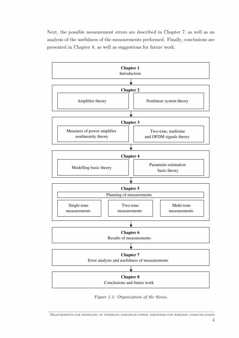
Next, the possible measurement errors are described in Chapter 7, as well as an
analysis of the usefulness of the measurements performed. Finally, conclusions are
presented in Chapter 8, as well as suggestions for future work.
Chapter 1
Introduction
Chapter 2
Nonlinear system theory
Measures of power amplifier
nonlinearity theory
Two-tone, multisine
and OFDM signals theory
Multi-tone
measurements
Single-tone
measurements
Chapter 5
Chapter 6
Results of measurements
Chapter 8
Conclusions and future work
Amplifier theory
Chapter 3
Two-tone
measurements
Planning of measurements
Chapter 7
Error analysis and usefulness of measurements
Chapter 4
Parameter estimation
basic theory Modelling basic theory
Figure 1.1: Organization of the thesis.
Measurements for modelling of wideband nonlinear power amplifiers for wireless communications
4
Chapter 2
Amplifiers
Amplifiers are very important components in modern wireless communications
systems, since they give the signal to be sent the necessary power to overcome the
losses that may occur during transmissions. However, they may also introduce
some problems, as the need of a higher system power and so, the need of batteries
that last longer, which bring along more expenses.
In general terms, an amplifier is an active component, which means that it does
not follow Ohm’s law [7] in a linear way and therefore, the output obtained from
it may vary according to the varying input signal.
In this chapter, the main concepts related to amplifiers are described. First, the
main definition of a power amplifier is given. Next, a comparison between tube
based and solid state amplifiers is done. Moreover, the most commonly used classes
of amplifiers are briefly described. Finally, the concepts of linearity and distortion
are reviewed for systems in general, as well as for the particular case of power
amplifiers.
Measurements for modelling of wideband nonlinear power amplifiers for wireless communications
5

2.1 Power amplifiers
A Power Amplifier (PA), increases the power of the input signal, so the voltage
and/or the current will be increased at the output of the device. Across the years,
different approaches have been taken in order to create the “perfect” power ampli-
fier. Nowadays, the most commonly used devices are the ones based on electron
beam tubes, usually Travelling Wave Tube Amplifiers (TWTA), and the Solid
State Power Amplifiers (SSPA) as shown in the Table 2.1, for different microwave
bandwidths.
Table 2.1: Types of amplifiers for different microwave frequency bands.
Name Frequency Band Solid State Type Tube Type
X-band 10.6 − 10.7 GHz 20 W (GaN device) 3000 W (TWT)Ka-band 22 − 36.5 GHz 6 W (0.15 µm
PHEMT devices)1000 W (Klystron)
Q-band 42.5 − 49.04 GHz 4 W -W-band 86 − 92 GHz 0.5 W (TRW) 1000 W (EIKA)
TWTA operation is based on the observations made by Thomas Alva Edison [8]
in 1879 when he invented the incandescent electric light bulb making an electric
current flow through a glass tube surrounding a vacuum. A schematic of a simple
TWTA is shown in Figure 2.1.
RF RF
anode
Figure 2.1: Basic TWTA [9].
At the left of Figure 2.1 there is an “electron gun”, which mainly consists of a
heater, a cathode and an anode. When heated, the cathode emits a stream of elec-
trons which passes through the anode and travels as a narrow beam through the
helix at the speed of light. The electron beam will transfer its energy to a signal
(electromagnetic wave) travelling along the helix amplifying it. By adjusting the
Measurements for modelling of wideband nonlinear power amplifiers for wireless communications
6
length of the helix and pitch it is possible to manipulate different operating fre-
quencies. Because of their construction, TWTAs offer large currents and therefore,
high output powers can be obtained.
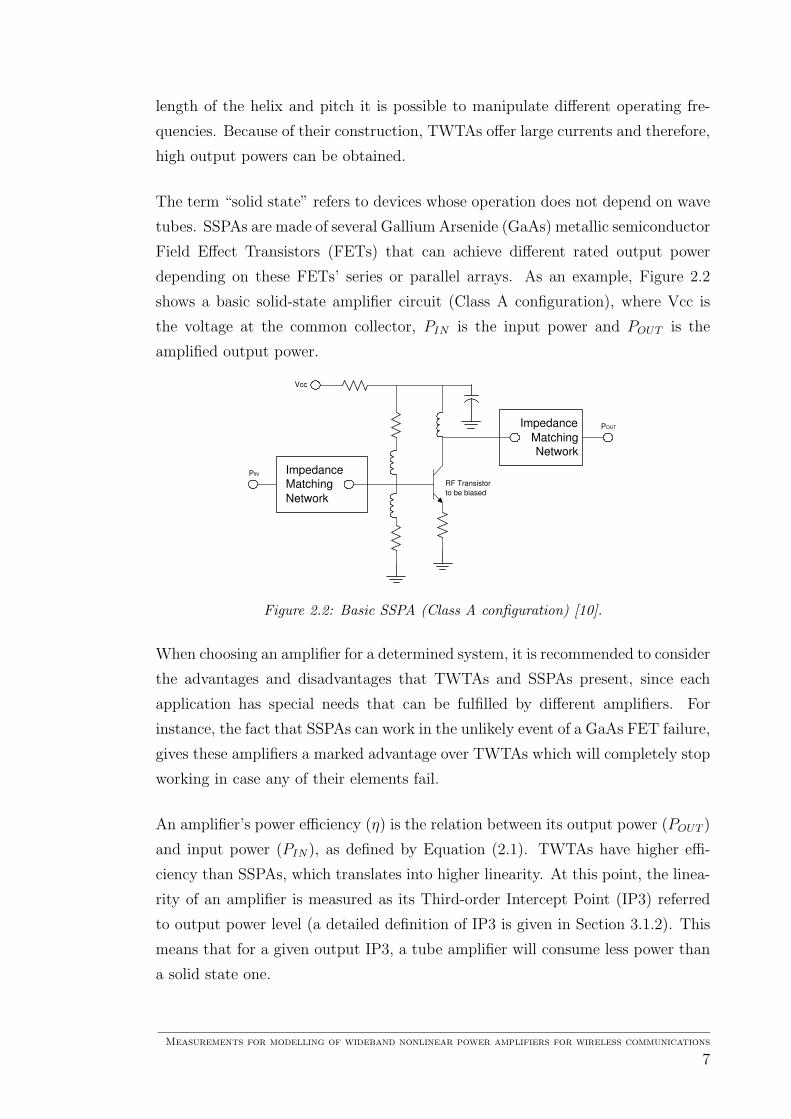
The term “solid state” refers to devices whose operation does not depend on wave
tubes. SSPAs are made of several Gallium Arsenide (GaAs) metallic semiconductor
Field Effect Transistors (FETs) that can achieve different rated output power
depending on these FETs’ series or parallel arrays. As an example, Figure 2.2
shows a basic solid-state amplifier circuit (Class A configuration), where Vcc is
the voltage at the common collector, PIN is the input power and POUT is the
amplified output power.
Impedance
Matching
Network
Impedance
Matching
Network
Vcc
P IN
P OUT
RF Transistor
to be biased
Figure 2.2: Basic SSPA (Class A configuration) [10].
When choosing an amplifier for a determined system, it is recommended to consider
the advantages and disadvantages that TWTAs and SSPAs present, since each
application has special needs that can be fulfilled by different amplifiers. For
instance, the fact that SSPAs can work in the unlikely event of a GaAs FET failure,
gives these amplifiers a marked advantage over TWTAs which will completely stop
working in case any of their elements fail.
An amplifier’s power efficiency (η) is the relation between its output power (POUT )
and input power (PIN), as defined by Equation (2.1). TWTAs have higher effi-
ciency than SSPAs, which translates into higher linearity. At this point, the linea-
rity of an amplifier is measured as its Third-order Intercept Point (IP3) referred
to output power level (a detailed definition of IP3 is given in Section 3.1.2). This
means that for a given output IP3, a tube amplifier will consume less power than
a solid state one.
Measurements for modelling of wideband nonlinear power amplifiers for wireless communications
7
η =POUT
PIN
(2.1)
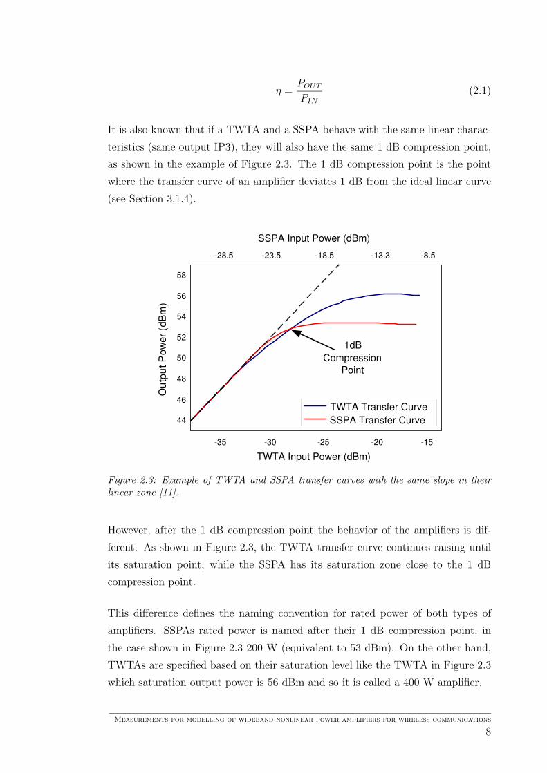
It is also known that if a TWTA and a SSPA behave with the same linear charac-
teristics (same output IP3), they will also have the same 1 dB compression point,
as shown in the example of Figure 2.3. The 1 dB compression point is the point
where the transfer curve of an amplifier deviates 1 dB from the ideal linear curve
(see Section 3.1.4).
58
56
54
52
50
48
46
44
-35 -30 -25 -20 -15
1dB
Compression
Point
TWTA Transfer Curve
SSPA Transfer Curve
-28.5 -23.5 -18.5 -13.3 -8.5
TWTA Input Power (dBm)
SSPA Input Power (dBm)
O u t p
u t
P o
w e
r ( d
B m
)
Figure 2.3: Example of TWTA and SSPA transfer curves with the same slope in theirlinear zone [11].
However, after the 1 dB compression point the behavior of the amplifiers is dif-
ferent. As shown in Figure 2.3, the TWTA transfer curve continues raising until
its saturation point, while the SSPA has its saturation zone close to the 1 dB
compression point.
This difference defines the naming convention for rated power of both types of
amplifiers. SSPAs rated power is named after their 1 dB compression point, in
the case shown in Figure 2.3 200 W (equivalent to 53 dBm). On the other hand,
TWTAs are specified based on their saturation level like the TWTA in Figure 2.3
which saturation output power is 56 dBm and so it is called a 400 W amplifier.
Measurements for modelling of wideband nonlinear power amplifiers for wireless communications
8
The transfer curve of a specific amplifier type presents in itself an advantage for
tube type amplifiers. Typically, SSPAs are operated in levels below its 1 dB
compression point. However, TWTAs have a “power reserve” in case of high path
loss as in rainy environments. This makes TWTAs more robust than SSPAs for
uncertain environmental conditions.
For amplitude and phase transfer characteristics, both types of amplifiers present
the same linearity pattern [11]. SSPAs behave better than TWTAs before their
common 1 dB compression point and at higher input power levels, when SSPAs
are already saturated, TWTAs have a better performance. This relationship may
also be applied from the cost point of view in order to choose a type of amplifier
to be used.
With respect to modular design of amplifiers, SSPAs give a more reliable scenario
than TWTAs. SSPAs have the ability of continuing working even when a fail occurs
in one of its modules, in which case it will continue operating at a lower output
power. According to the “static reliability analysis” proposed in [12], TWTAs can
only have 71% of the reliability of SSPAs, based on their architecture and having
the same reliability for all their subsystems.
Another important aspect to consider in modular design is the power supply needed
to operate the amplifiers. In this, SSPAs have a marked advantage since there
exist many devices that are able to fulfill their operating voltage needs, which are
typically a few volts (between +12 V and +50 V) in contrast with TWTAs, which
require supplies of several thousands of volts that can be very difficult to find and
complex to build.
From the cost point of view, building a modular TWTA is extremely difficult and
expensive because of the complexity of the vacuum tube architecture. Moreover,
there are not power supplies at the high voltage levels required by travelling tubes
available in nowadays market. Consequently, for the same output power levels,
it is possible to build a modular SSPA for the same cost than for an equivalent
TWTA.
Even though SSPAs have several advantages on TWTAs, we should also consider
that the last ones are more efficient and less expensive when used at low frequencies.
Besides, tube amplifiers are widely recommended for professional audio applica-
Measurements for modelling of wideband nonlinear power amplifiers for wireless communications
9

tions (guitar amplifiers, microphone preamplifiers, equalizers, etc.) due to their
specific distortion and speaker-damping characteristics, which are very difficult to
imitate with SSPAs.
As mentioned before, the specific characteristics of each type of amplifiers should
be taken on count when choosing one to be used in a specific system. Their ad-
vantages and disadvantages are summarized in Table 2.2.
Table 2.2: TWTAs compared to SSPAs.
TWTA SSPA
Advantages ¦ Amplifies a wide range offrequencies at the same time
¦ Physically small
¦ Excellent performance inaudio and satellite devices
¦ Amplifies in stages
¦ Efficient and less expensivefor high power outputs(>10 kW) and highfrequencies (>50 MHz)
¦ Can continue working whenpartial failures occur
Disadvantages ¦ Difficult to repair ¦ High power consumption¦ More expensive and complex
power supply required¦ Instabilities due to failures
¦ Shorter active life (4 to 6years)
¦ Not recommended for lowfrequencies
Applications ¦ High power applications(e.g. remote sensing)
¦ Low and medium powerapplications (e.g. space-flight)
¦ Earth stations andcommunication satellites
¦ AM and FM broadcasttransmitters
¦ Professional audio(e.g. microphones, limiters,equalizers)
¦ TV, HF/VHF, lower powerUHF, OFDM and HDTVbroadcast
¦ High-power UHF TV stations ¦ Telecommunications¦ FM broadcast stations ¦ Broadband and wireless RF
Guitar amplifiers ¦ Radar¦ Cellular-telephone handsets¦ Base station transmitters
Measurements for modelling of wideband nonlinear power amplifiers for wireless communications
10
2.2 Classes of amplifiers
Power amplifiers can be classified based on their rated power as low (below 1 mW),
medium (from 1 mW to 10 W) or high (above 10 W). However, it is very popular
to use a “class” method to categorize them [13], based on, for example, their circuit
configurations, operational topology, linearity and efficiency. Examples of the so-
called linear power amplifier classes are A, B, AB and C, the most commonly used
nowadays. These classes represent the amount of variation that the output signal
presents in a complete operation cycle of the input signal.
Other classes of amplifiers briefly discussed are D, E, F, G, H and S, which are
more recent approaches to improve Class B or C amplifiers [14]. These last classes
are better known as switched mode amplifiers, because of its way of operate, or as
nonlinear power amplifiers, due to their poor linearity performance. However, they
can achieve higher efficiency and their linearity can be improved using linearization
techniques.
An important concept used to place an amplifier into a specific class is efficiency. As
mentioned in Section 2.1, an amplifier’s power efficiency is defined as the relation
between output power and input power. This ratio is a good measurement for
amplifiers when choosing one for a specific application, since it tells how much
power is spent and this can be easily related with the budget of a project.
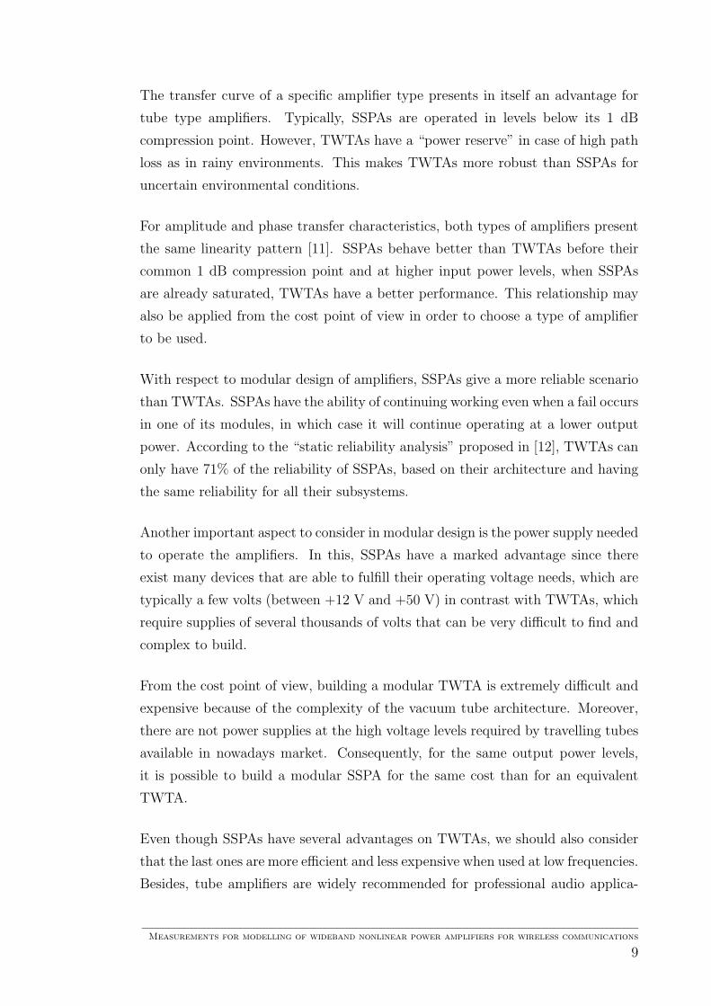
In Class A amplifiers, the output signal varies through the complete cycle of the
input signal. They operate at constant current, independently of the input signal
level and at all times. Then, the DC current must be at least equal to the peak
output current (Figure 2.4). Because of this, they are expensive when transmitting
signals that have large peak-to-average signal power and also, their efficiency is
limited to just 25%.
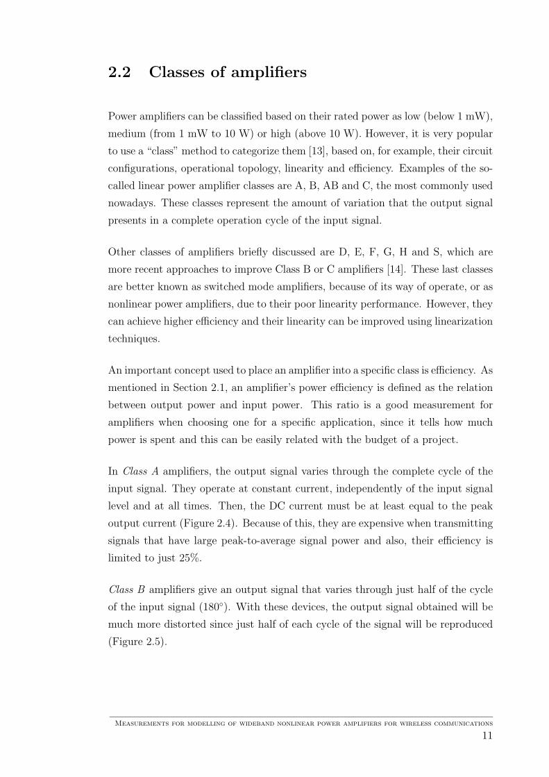
Class B amplifiers give an output signal that varies through just half of the cycle
of the input signal (180). With these devices, the output signal obtained will be
much more distorted since just half of each cycle of the signal will be reproduced
(Figure 2.5).
Measurements for modelling of wideband nonlinear power amplifiers for wireless communications
11
- Gate Voltage
Bias
Input
Signal
D r a
i n
C u
r r e n t
Output
Signal Cut-off
point
Figure 2.4: Class A amplifier’s operation point.
In order to make class B amplifiers more useful, a “push-pull” output stage is
used, which has two valves that operate for each half-cycle of the input signal (one
for the positive and another for the negative). With this system, we can obtain a
maximum efficiency of 78.5%, which is better than for Class A. However, due to
the system used of two valves, some crossover distortion may be introduced, which
might not be desirable in most applications.
- Gate Voltage
D r a
i n
C u
r r e n t
Input
Signal
Bias
and Cut-off point
Output
Signal
Figure 2.5: Class B amplifier’s operation point.
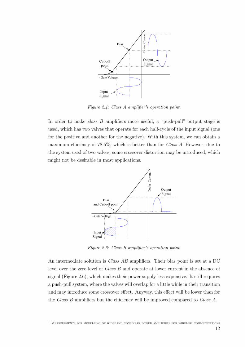
An intermediate solution is Class AB amplifiers. Their bias point is set at a DC
level over the zero level of Class B and operate at lower current in the absence of
signal (Figure 2.6), which makes their power supply less expensive. It still requires
a push-pull system, where the valves will overlap for a little while in their transition
and may introduce some crossover effect. Anyway, this effect will be lower than for
the Class B amplifiers but the efficiency will be improved compared to Class A.
Measurements for modelling of wideband nonlinear power amplifiers for wireless communications
12

- Gate Voltage
D r a
i n
C u
r r e n t
Input
Signal
Output
Signal
Bias
Cut-off
point
Figure 2.6: Class AB amplifier’s operation point.
The output of a Class C amplifier is biased to operate at less than 180 of the input
cycle and only with a tuned resonant circuit that gives a complete operation cycle
for the tuned or resonant frequency. Because of this, these amplifiers are used in
very special tuned circuit areas such as radio communications. Their theoretical
efficiency is very high (even 100% can be achieved). However, it is not common
to use them to produce high power levels and they tend to be very expensive to
build because of the need of high-performance transistors.
In order to make comparison easier, the main characteristics of the linear amplifier
classes presented are summarized in Table 2.3.
Table 2.3: Classes of linear amplifiers.
Class A Class AB Class B Class C
Conduction Both More than One polarity Peak of oneangle polarities one polarity (180) polarity
(180) (> 180) (< 180)
RF Gain High High /Moderate
Moderate Low
RF Power High High High LowDrain Low Moderate High Very highefficiency (≤ 25%) (25%-78.5%) (≤ 78.5%) (78.5%-100%)
Non-linearities
Low Moderate High Very high
Operationfrequency
High Moderate Low Very low
Measurements for modelling of wideband nonlinear power amplifiers for wireless communications
13

Class D amplification uses digital pulses that are “on” for a short interval of time
and “off” for a longer time (switched mode amplifier). The use of digital techniques
allows obtaining a signal that may vary through the complete input cycle (using
sampling and retention circuits) to produce an output signal based on several parts
of the input signal. The main advantage of these amplifiers is that they are “on”
(using power) just for short intervals and the general efficiency may be very high
(usually higher than 90%).
In the operation of Class E amplifiers, the transistor works as an ideal switch
without “on” resistance and infinite “off” resistance. This switching produces
distortion, which may be translated as nonlinearities. An important characteristic
of this class is that it employs an output network that shapes the waveforms
of voltage and current to avoid simultaneous high voltage and high current in
the transistor, which produces high efficiency [15]. Their ideal efficiency is 100%
although, in practice, factors as saturation voltage and switching time reduce it.
Compared to Class E, Class F amplifiers do not require a fast switching driver sig-
nal and their implementation is easier. These amplifiers use a resonating network
[14] to control their voltage and current waveforms, reducing their transistors’
power dissipation and increasing their efficiency. When setting their operation
point at the cutoff region for switching operation, they are able to achieve an
efficiency of 100%.
Class G amplifiers are widely used in audio applications, where a narrow band-
width is not required. These amplifiers require more than one voltage source and
two or more pairs of active devices, which make the bandwidth of the whole device
wide. Out of these devices, low power transistors handle the amplification most of
the time and the high power ones switch only during peak signal demand. Their
optimal efficiency (close to 100%) is achieved when used with signals that do not
need high voltage supply (low level signals).
Class H amplifiers are based on Class G and, as those, they are used mainly in
audio products. These amplifiers work with two different supply voltages, which
are switched “on” as required, depending on the size of the signal being amplified.
This allows the power supply to track the input signal and provide just enough
voltage for the output signal. Their efficiency, as in Class G amplifiers, may be
made close to 100%.
Measurements for modelling of wideband nonlinear power amplifiers for wireless communications
14
Finally, the Class S, also called “switching regulator”, is based on Class D am-
plifiers. It uses Pulse-Width Modulation (PWM) [14], which basic operation is
to create a variable duty-cycle (varying the mean levels) to form a rectangular
waveform. Therefore, Class S amplifiers are used also as amplitude modulators.
The rectangular PWM voltage waveform is applied to a low-pass filter in order to
reduce distortion, increasing the efficiency compared to Class D amplifiers.
2.3 Linearity and distortion
In order to understand the need of linear amplifiers in modern communication
systems, it is important to define what is meant by linearity. In general, a linear
system is the one whose output is proportional to its input, meaning that the form
of the output signal will be the same than the input, affected by a constant factor
k. When k = 1, the output will be an exact replica of the input. Otherwise, if
k > 1, the amplitude of the output signal will be increased (amplified) with respect
to the input and if k < 1, it will be reduced.
Mathematically, a system is said to be linear when it accomplishes the superposi-
tion property, which combines the additivity and scalability concepts, as defined in
Equation (2.2). The additivity property means that the output of a system which
input is the sum of several signals will be the sum of the individual outputs of
each signal when applied to the same system. On the other hand, the scalability
principle simply means that, in a linear system, the response to αx1(t) will be
αy1(t), where α is any complex constant.
x(t) = α1x1(t) + α2x2(t) ⇒ y(t) = α1y1(t) + α2y2(t) (2.2)
When distortion occurs, the output is not an exactly scaled version of the input
signal. This distortion can be caused by the nonlinear characteristics of the device,
which is called nonlinear or amplitude distortion. This may happen with all classes
of amplifiers presented in Section 2.2. The distortion may occur as well because
the elements of a system or a device have different behavior related to the input
signal at different frequencies, being referred to as frequency distortion.
Measurements for modelling of wideband nonlinear power amplifiers for wireless communications
15
Other kinds of distortion may be introduced to the transmitted signal in the form
of noise inside the frequency band, which may generate additional frequency com-
ponents in adjacent channels [16].
In general, distortion can be classified as memoryless distortion (instantaneous)
or distortion with memory. When referring to memoryless distortion, the output
depends only on the instantaneous input value. In the case of distortion with
memory, the output depends not only on the instantaneous input value but also
on the previous ones [17].
Nonlinear amplifiers are devices with memory, since they contain components
that store energy, such as capacitors and inductors. Therefore, it results more
accurate to classify systems that contain amplifiers into frequency-independent
or frequency-dependent systems. Frequency-independent systems can be with or
without memory, while frequency-dependent systems always contain memory com-
ponents. This classification is useful when modelling the nonlinearity of power
amplifiers [5].
2.4 Distortion in power amplifiers
An ideal power amplifier would have a linear transfer characteristic as shown in
Figure 2.7(a), which can be represented by Equation (2.3), where K is the power
gain. This means that the output power (POUT ) would be a multiple of the input
power (PIN) and, consequently, the shape of the input and output signals is exactly
the same.
Mathematically, distortion due to an amplifier occurs when adding second, third or
higher terms to the ideal transfer characteristic of Equation (2.3), resulting in one
of the form shown in Equation (2.4). This means that the output signal will have
a different shape than the input. This is the common case since in practice 100%
linear amplifiers do not exist. The transfer characteristic of a nonlinear amplifier
is illustrated in Figure 2.7(b).
Measurements for modelling of wideband nonlinear power amplifiers for wireless communications
16

P IN (t)
P O
U T
( t )
0
0
Slope = K
(a) Ideal amplifier
P IN (t)
P O
U T
( t )
Cut-off zone Linear zone Saturation zone
0
0
(b) Nonlinear amplifier
Figure 2.7: Transfer characteristic of an amplifier.
POUT (t) = K PIN(t) (2.3)
POUT (t) = K1PIN(t) + K2P2IN(t) + K3P
3IN(t) + K4P
4IN(t) + K5P
5IN(t) + · · · (2.4)
Notice that the transfer characteristic of a nonlinear amplifier has three main zones,
as shown in Figure 2.7(b). In the cut-off region an amplifier will act as an open
circuit, since the bias is not sufficient for conduction to occur. When increasing the
bias, the amplifier will enter the linear zone, where it will act as a linear amplifier,
achieving the specified maximum gain. However, if the bias is further increased,
the amplifier will saturate, meaning that high amplitude signals will not respond
to increased gain and will appear flattened (distorted).
Measurements for modelling of wideband nonlinear power amplifiers for wireless communications
17
2.5 Summary of the chapter
In this chapter basic theory about amplifiers is summarized. First, the advantages
and disadvantages between the two most commonly used types of amplifiers were
given. The older type, travelling wave tube amplifiers, have an excellent perfor-
mance when high power outputs and high frequencies are needed. However, solid
state amplifiers have become popular in the last decades due to their physical small
size and their reliability in communication applications.
Next, the classes of amplifiers were described, including their topology, operation
and efficiency. Classes A, B, AB and C are the most widely used, from which Class
C amplifiers have the highest efficiency and linearity but they can just provide low
gain amplification.
Finally, the general concepts of linearity and distortion were briefly explained and
described by a graphical example. Moreover, the distortion effect introduced by
amplifiers was mathematically characterized as the addition of second- or higher-
order terms to their linear transfer characteristic.
Measurements for modelling of wideband nonlinear power amplifiers for wireless communications
18

Chapter 3
Power amplifier distortion
measures
In order to model the nonlinearity produced by power amplifiers, it is necessary to
understand different types of distortion caused by them. Moreover, the techniques
to determine the level of the distortion should be considered in order to obtain the
adequate parameters for modelling.
A nonlinear amplifier can distort the signal passing through the amplifier and, in
addition, signals in adjacent channels or bands [14]. Amplifier distortion can be
divided into two main groups: generation of harmonic components and generation
of intermodulation products or Intermodulation Distortion (IMD).
The distortion based on generation of harmonic components occurs when a simple
one frequency (single-tone) signal propagates through a nonlinear device. If these
harmonic components are not filtered away, they will affect nearby channels or
bands. On the other hand, IMD is generated when more than one frequency (multi-
tone) signal is applied to the system, producing frequency components inside the
signal’s fundamental frequency band, which are difficult to filter out.
In this chapter, the specific distortion caused by power amplifiers when working
with different signals is presented. This includes the parameters for modelling
purposes that can be obtained from each type of signal (single-, two- or multi-
tone), as well as the description an graphical example of each type of nonlinearity.
Measurements for modelling of wideband nonlinear power amplifiers for wireless communications
19

3.1 Distortion measures using single-tone signals
As earlier mentioned, single-tone signals passing through a nonlinear amplifier
produce harmonic components, which will appear at multiple frequencies of the
fundamental frequency. Usually, the frequencies where these components appear
are outside the system frequency band and therefore, it is easy to eliminate them
using a lowpass filter. If a filter is not used, adjacent channel interference will be
present in the general system.
3.1.1 Second harmonic distortion
The simplest model of amplitude nonlinearity occurs when a term proportional to
the square of the input power is added to the transfer characteristic, resulting in
Equation (3.1).
POUT (t) = K1 PIN(t) + K2 P 2IN(t) (3.1)
This type of nonlinearity is called second harmonic distortion since an additional
frequency component will appear at twice the original frequency in the spectrum
of the output signal. The amplitude of this component will be proportional to the
coefficient of the quadratic term. Furthermore, this type of distortion will also
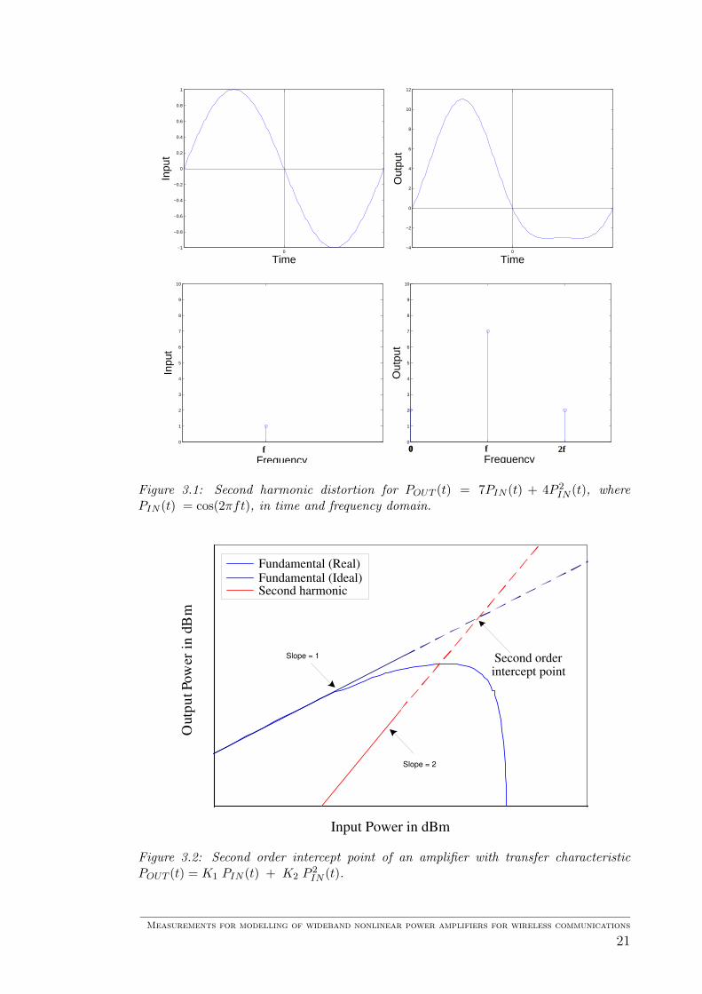
produce a DC component in the transfer characteristic. Figure 3.1 illustrates an
example of an amplifier’s characteristic with a second harmonic distortion, in time
and frequency domain, where f is the fundamental frequency.
It is evident that the amplitude of the second harmonic distortion increases pro-
portionally to the square of the input signal and the constant K2, while the ampli-
tude of the fundamental characteristic increases only in function of the constant
K1. The point where these two amplitudes are the same is called second order
Intercept Point (IP2) and is useful to calculate the distortion level at a specific
input level.
The second order intercept point of a nonlinear amplifier is shown in Figure 3.2.
Notice that the lines are dotted at high input levels, meaning that at very high
input levels it is impossible to measure a nonlinear amplifier without destroying it
and therefore, only theoretical representation can be done.
Measurements for modelling of wideband nonlinear power amplifiers for wireless communications
20
0−1
−0.8
−0.6
−0.4
−0.2
0
0.2
0.4
0.6
0.8
1
Time
Inpu
t
0 −4
−2
0
2
4
6
8
10
12
Time
Out
put
0
1
2
3
4
5
6
7
8
9
10
Frequency
Inpu
t
f 0
1
2
3
4
5
6
7
8
9
10
Frequency
Out
put
f 0 0 2f
Figure 3.1: Second harmonic distortion for POUT (t) = 7PIN (t) + 4P 2IN (t), where
PIN (t) = cos(2πft), in time and frequency domain.
Second order intercept point
O u
t p u
t P
o w
e r
i n d
B m
Input Power in dBm
Fundamental (Ideal) Second harmonic
Slope = 2
Slope = 1
Fundamental (Real)
Figure 3.2: Second order intercept point of an amplifier with transfer characteristicPOUT (t) = K1 PIN (t) + K2 P 2
IN (t).
Measurements for modelling of wideband nonlinear power amplifiers for wireless communications
21
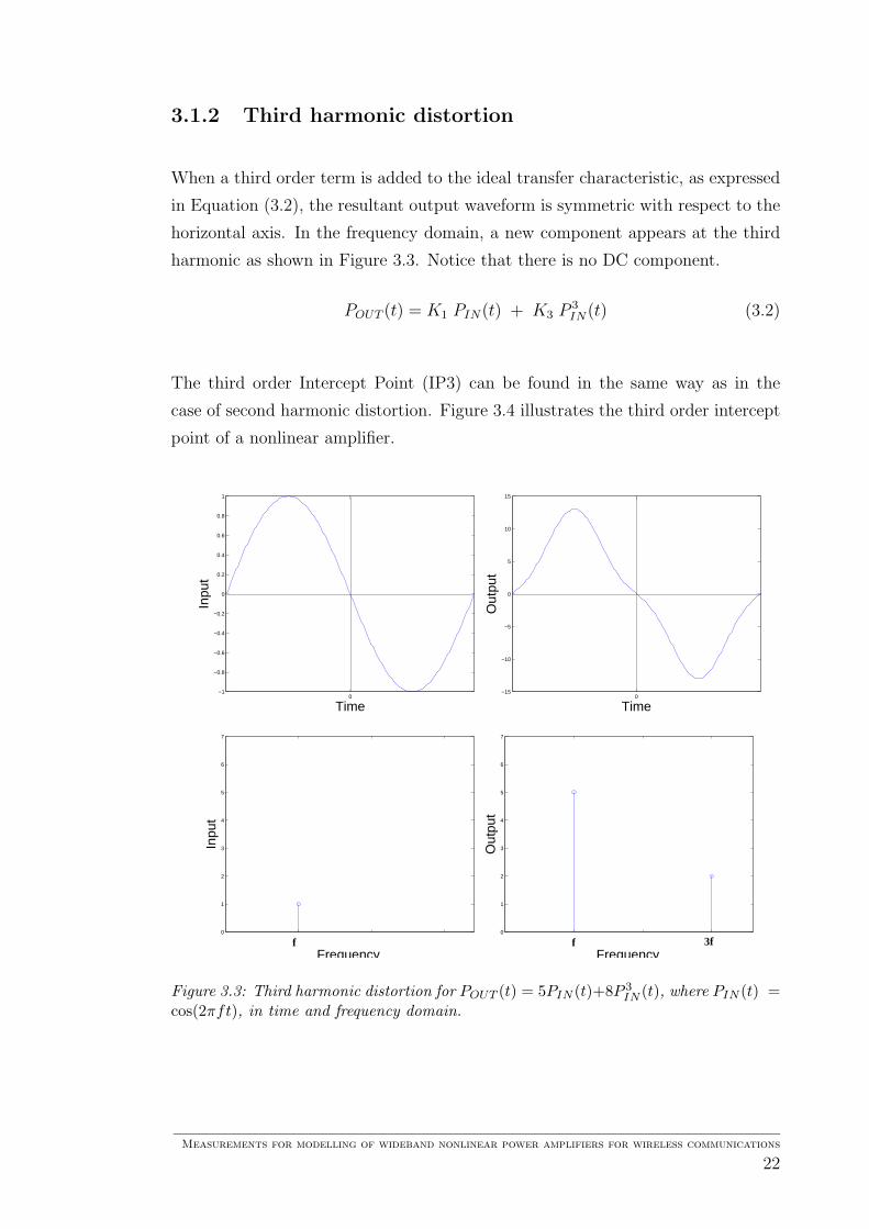
3.1.2 Third harmonic distortion
When a third order term is added to the ideal transfer characteristic, as expressed
in Equation (3.2), the resultant output waveform is symmetric with respect to the
horizontal axis. In the frequency domain, a new component appears at the third
harmonic as shown in Figure 3.3. Notice that there is no DC component.
POUT (t) = K1 PIN(t) + K3 P 3IN(t) (3.2)
The third order Intercept Point (IP3) can be found in the same way as in the
case of second harmonic distortion. Figure 3.4 illustrates the third order intercept
point of a nonlinear amplifier.
0−1
−0.8
−0.6
−0.4
−0.2
0
0.2
0.4
0.6
0.8
1
Time
Inpu
t
0−15
−10
−5
0
5
10
15
Time
Out
put
0
1
2
3
4
5
6
7
Frequency
Inpu
t
f0
1
2
3
4
5
6
7
Frequency
Out
put
f 3f
Figure 3.3: Third harmonic distortion for POUT (t) = 5PIN (t)+8P 3IN (t), where PIN (t) =
cos(2πft), in time and frequency domain.
Measurements for modelling of wideband nonlinear power amplifiers for wireless communications
22
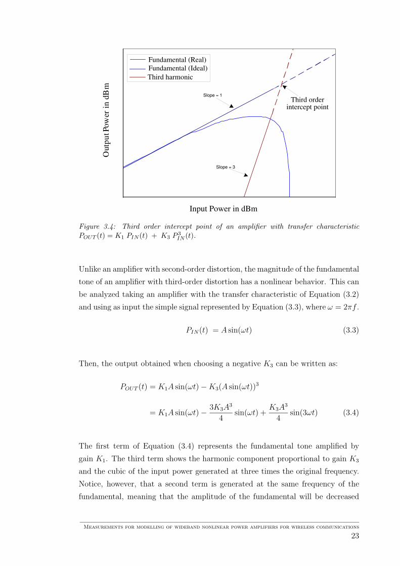
Third order intercept point
O u
t p u
t P
o w
e r
i n d
B m
Input Power in dBm
Fundamental (Real)
Fundamental (Ideal)
Third harmonic
Slope = 1
Slope = 3
Figure 3.4: Third order intercept point of an amplifier with transfer characteristicPOUT (t) = K1 PIN (t) + K3 P 3
IN (t).
Unlike an amplifier with second-order distortion, the magnitude of the fundamental
tone of an amplifier with third-order distortion has a nonlinear behavior. This can
be analyzed taking an amplifier with the transfer characteristic of Equation (3.2)
and using as input the simple signal represented by Equation (3.3), where ω = 2πf .
PIN(t) = A sin(ωt) (3.3)
Then, the output obtained when choosing a negative K3 can be written as:
POUT (t) = K1A sin(ωt) − K3(A sin(ωt))3
= K1A sin(ωt) − 3K3A3
4sin(ωt) +
K3A3
4sin(3ωt) (3.4)
The first term of Equation (3.4) represents the fundamental tone amplified by
gain K1. The third term shows the harmonic component proportional to gain K3
and the cubic of the input power generated at three times the original frequency.
Notice, however, that a second term is generated at the same frequency of the
fundamental, meaning that the amplitude of the fundamental will be decreased
Measurements for modelling of wideband nonlinear power amplifiers for wireless communications
23
proportionally to the cubic of the input signal. This gives the characteristic form of
the transfer function of an amplifier where a third order nonlinearity predominates,
as the one shown in Figure 3.4.
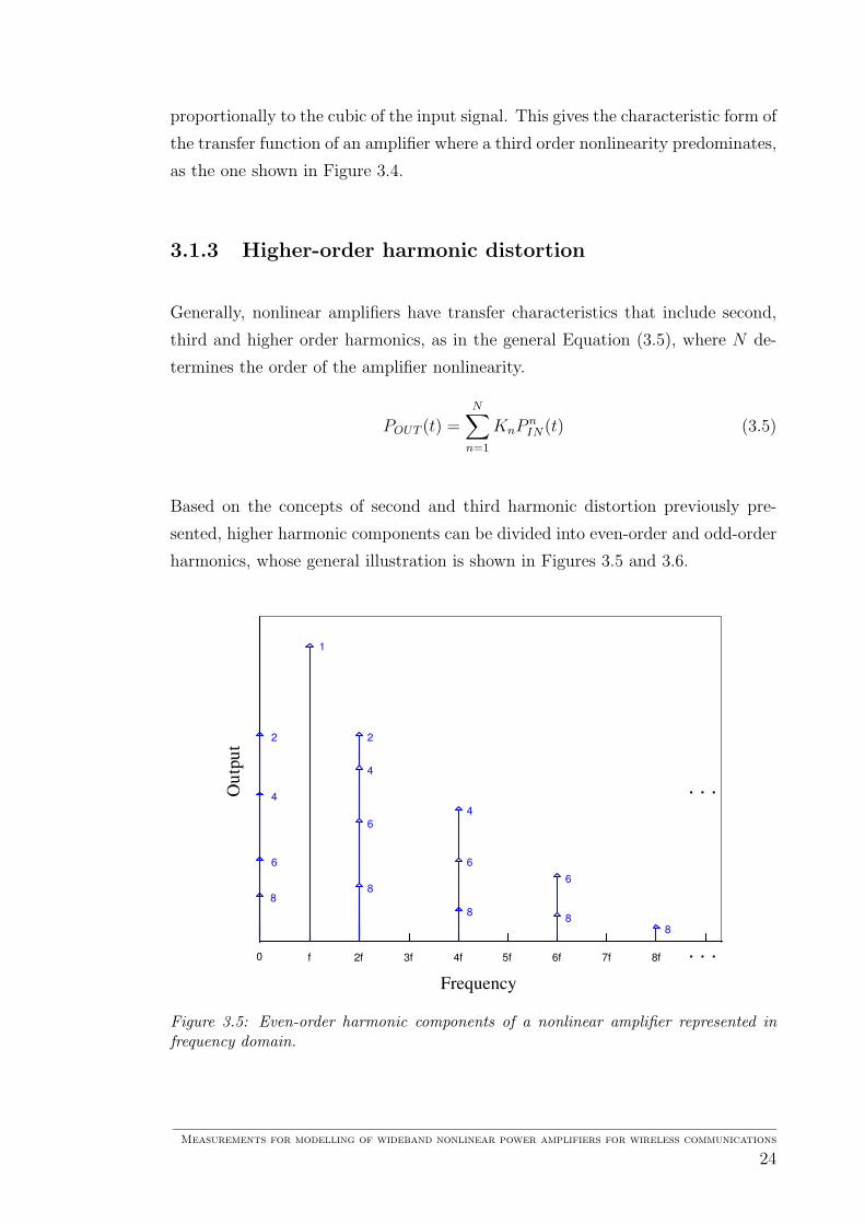
3.1.3 Higher-order harmonic distortion
Generally, nonlinear amplifiers have transfer characteristics that include second,
third and higher order harmonics, as in the general Equation (3.5), where N de-
termines the order of the amplifier nonlinearity.
POUT (t) =N
∑
n=1
KnPnIN(t) (3.5)
Based on the concepts of second and third harmonic distortion previously pre-
sented, higher harmonic components can be divided into even-order and odd-order
harmonics, whose general illustration is shown in Figures 3.5 and 3.6.
O u
t p u t
Frequency
2f 3f 4f 5f 6f 7f 8f f
. . .
0
2
4
6
8 8
8
8 8
6
6
6
4
4
2
1
. . .
Figure 3.5: Even-order harmonic components of a nonlinear amplifier represented infrequency domain.
Measurements for modelling of wideband nonlinear power amplifiers for wireless communications
24
O u
t p u t
Frequency
2f 3f 4f 5f 6f 7f 8f f
. . .
0
1
. . . 7
7
7 5
5
3 7
5
3
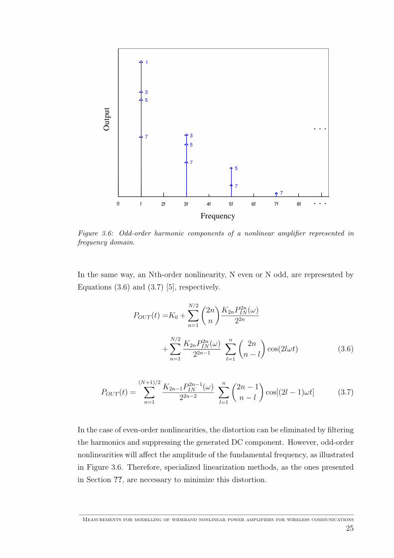
Figure 3.6: Odd-order harmonic components of a nonlinear amplifier represented infrequency domain.
In the same way, an Nth-order nonlinearity, N even or N odd, are represented by
Equations (3.6) and (3.7) [5], respectively.
POUT (t) =K0 +
N/2∑
n=1
(
2n
n
)
K2nP2nIN(ω)
22n
+
N/2∑
n=1
K2nP 2nIN(ω)
22n−1
n∑
l=1
(
2n
n − l
)
cos(2lωt) (3.6)
POUT (t) =
(N+1)/2∑
n=1
K2n−1P2n−1IN (ω)
22n−2
n∑
l=1
(
2n − 1
n − l
)
cos[(2l − 1)ωt] (3.7)
In the case of even-order nonlinearities, the distortion can be eliminated by filtering
the harmonics and suppressing the generated DC component. However, odd-order
nonlinearities will affect the amplitude of the fundamental frequency, as illustrated
in Figure 3.6. Therefore, specialized linearization methods, as the ones presented
in Section ??, are necessary to minimize this distortion.
Measurements for modelling of wideband nonlinear power amplifiers for wireless communications
25
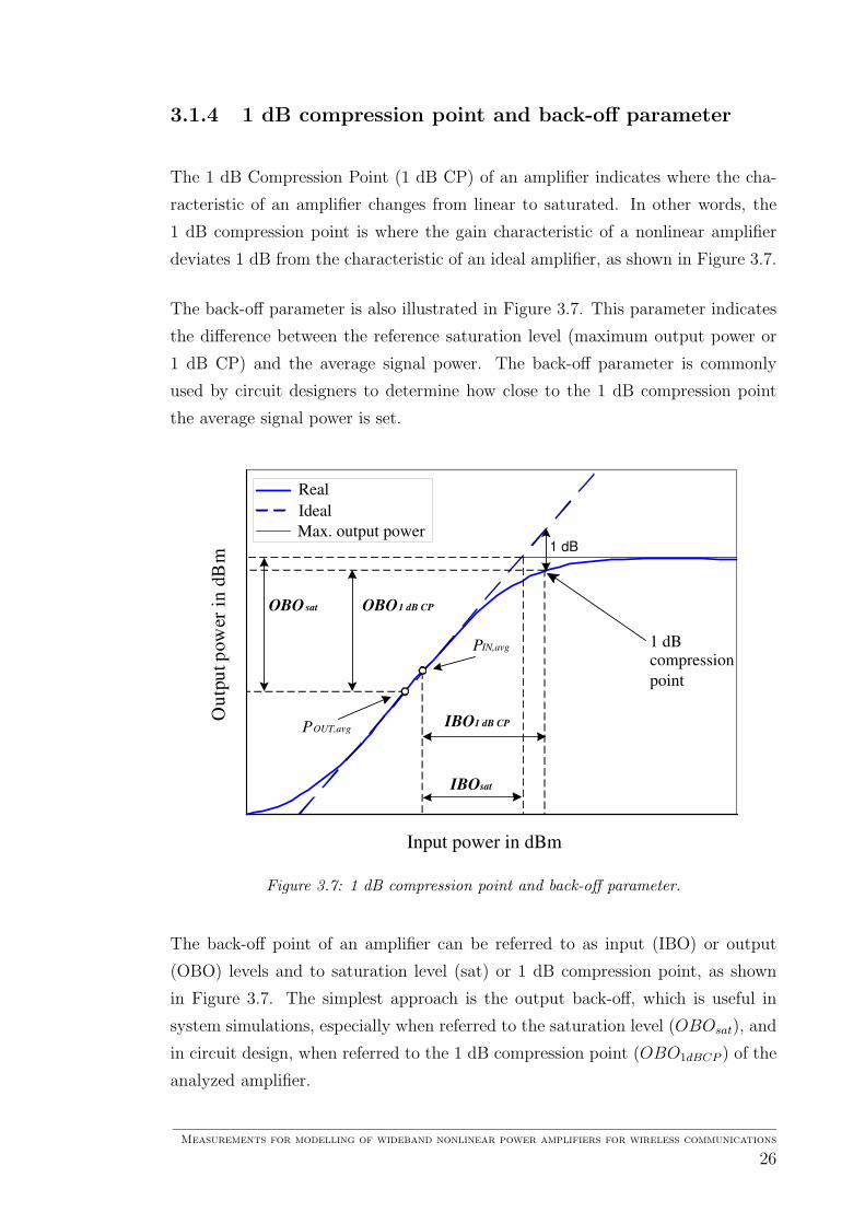
3.1.4 1 dB compression point and back-off parameter
The 1 dB Compression Point (1 dB CP) of an amplifier indicates where the cha-
racteristic of an amplifier changes from linear to saturated. In other words, the
1 dB compression point is where the gain characteristic of a nonlinear amplifier
deviates 1 dB from the characteristic of an ideal amplifier, as shown in Figure 3.7.
The back-off parameter is also illustrated in Figure 3.7. This parameter indicates
the difference between the reference saturation level (maximum output power or
1 dB CP) and the average signal power. The back-off parameter is commonly
used by circuit designers to determine how close to the 1 dB compression point
the average signal power is set.
O u
t p u t
p o
w e r
i n d
B m
Input power in dBm
1 dB compression
point
Real
Ideal
1 dB Max. output power
P IN,avg
P OUT,avg
OBO sat OBO 1 dB CP
IBO sat
IBO 1 dB CP
Figure 3.7: 1 dB compression point and back-off parameter.
The back-off point of an amplifier can be referred to as input (IBO) or output
(OBO) levels and to saturation level (sat) or 1 dB compression point, as shown
in Figure 3.7. The simplest approach is the output back-off, which is useful in
system simulations, especially when referred to the saturation level (OBOsat), and
in circuit design, when referred to the 1 dB compression point (OBO1dBCP ) of the
analyzed amplifier.
Measurements for modelling of wideband nonlinear power amplifiers for wireless communications
26
In general, the output back-off is easily calculated with Equation (3.8), where
POUT,max is the maximum output power given by the amplifier (or the 1 dB CP
if referenced to it) and POUT,avg is the average signal power measured from the
output of the amplifier.
OBO = 10 log10
(
POUT,max
POUT,avg
)
(3.8)
The back-off parameter is calculated when a signal is introduced to an amplifier at
a specific bias point. This is not the case when doing single-tone signal measure-
ments, where input signals of different bias points are applied to the amplifier in
order to perform a power-sweep or frequency-sweep measurement. Consequently,
the back-off will not be calculated in this thesis but is recommended when testing
specific signals, such as modulated or noisy signals.
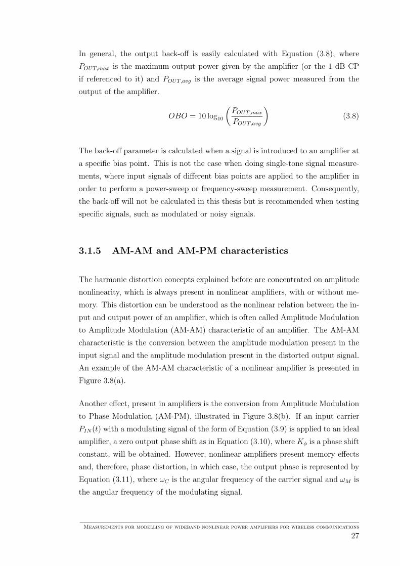
3.1.5 AM-AM and AM-PM characteristics
The harmonic distortion concepts explained before are concentrated on amplitude
nonlinearity, which is always present in nonlinear amplifiers, with or without me-
mory. This distortion can be understood as the nonlinear relation between the in-
put and output power of an amplifier, which is often called Amplitude Modulation
to Amplitude Modulation (AM-AM) characteristic of an amplifier. The AM-AM
characteristic is the conversion between the amplitude modulation present in the
input signal and the amplitude modulation present in the distorted output signal.
An example of the AM-AM characteristic of a nonlinear amplifier is presented in
Figure 3.8(a).
Another effect, present in amplifiers is the conversion from Amplitude Modulation
to Phase Modulation (AM-PM), illustrated in Figure 3.8(b). If an input carrier
PIN(t) with a modulating signal of the form of Equation (3.9) is applied to an ideal
amplifier, a zero output phase shift as in Equation (3.10), where Kφ is a phase shift
constant, will be obtained. However, nonlinear amplifiers present memory effects
and, therefore, phase distortion, in which case, the output phase is represented by
Equation (3.11), where ωC is the angular frequency of the carrier signal and ωM is
the angular frequency of the modulating signal.
Measurements for modelling of wideband nonlinear power amplifiers for wireless communications
27
O u
t p u t p
o w
e r
i n d
B m
Input power in dBm
Ideal
0
0
(a) AM-AM conversion
Input power in dBm
Ideal 0
0
O u
t p u t p
h a s e
i n
d e g
(b) AM-PM conversion
Figure 3.8: Amplitude and phase distortion of a nonlinear amplifier represented respec-tively AM-AM and AM-PM transfer characteristics.
M(t) = AM cos(ωM t) (3.9)
Φ(PIN(t)) = Kφ (3.10)
Φ(PIN(t)) = Kφ cos[ωCt + AM cos(ωM t)] (3.11)
In general, if an amplifier is operated in the linear region, AM-AM and AM-PM
characteristics are difficult to measure, since the harmonic components are very
small compared to the strong fundamental signal. Therefore, it is easier to measure
and analyze distortion tones as presented in the following sections.
3.1.6 Frequency sweep
The above measures represent instantaneous nonlinear characteristics of amplifiers.
Since they do not consider memory effects (other than AM-PM conversion), the
frequency-dependent behavior of the system cannot be described.
When describing narrowband devices, memory effects are often neglected since
they are very small compared to the device capabilities. However, in wideband
devices, memory effects can be strongly present and frequency-dependent models
will produce more accurate models.
Measurements for modelling of wideband nonlinear power amplifiers for wireless communications
28
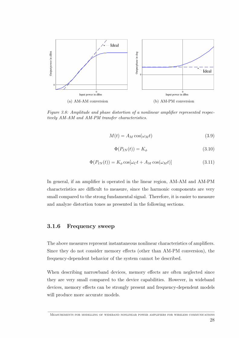
For this purpose, frequency-sweep measurements are used, where the gain and
output phase of the tested amplifier are swept throughout the whole frequency
band, as shown in Figures 3.9(a) and 3.9(b), where the frequency dependency of
the amplifier characteristics can be noticed.
The results of this kind of measurements are useful in modelling frequency-
dependent amplifiers with methods as Volterra series, Hammerstein, Wiener and
Saleh models as discussed in [5].
G a i n
Frequency
Operating
frequency band
0
(a) Gain characteristic
O u
t p u t
p h
a s e
Frequency
Operating
frequency band
0
0
(b) Phase characteristic
Figure 3.9: Frequency sweep of amplifier transfer characteristic.
3.2 Distortion measures using two-tone signals
In addition to harmonic components and compression, the output of an amplifier
that is fed with a multi-tone signal will contain intermodulation products or IMD,
which appear inside the fundamental frequency band and are, therefore, difficult
to filter away. Here, a two-tone signal is analyzed since it is the simplest possible
multi-tone signal and because a very well known method to measure amplifiers,
the two-tone test, is based on it.
In a two-tone test, a signal like the one defined by Equation (3.12) and depicted in
Figure 3.10 is applied to the Device Under Test (DUT). The envelope of this input
signal is varied throughout its complete range in order to test the whole transfer
characteristic of the DUT.
Measurements for modelling of wideband nonlinear power amplifiers for wireless communications
29

PIN(t) = A1cos(ω1t) + A2cos(ω2t) (3.12)
0
0
Time
Am
plitu
de
(a) Time domain
0
Frequency
Am
plitu
de
(b) Frequency domain
Figure 3.10: Illustration of a two-tone signal.
3.2.1 Intermodulation products
In general, when a two-tone signal is applied to a nonlinear amplifier, harmonic
zones will be generated, as explained in the previous section. Furthermore, new
frequencies called Intermodulation Products (IMP) will be presented and will be
of the form shown in Equation (3.13) [14], where f1 and f2 are the frequencies of
the two input tones, m and n are positive integers (excluding zero) and m + n is
equal to the order of the amplifier nonlinearity.
fIMP = m f1 ± n f2 (3.13)
According to Equation (3.13), when a two-tone signal is applied to an amplifier
with second order transfer characteristic, additional frequency components will
appear at f2 − f1 and f1 + f2. Additionally, each of the two input tones will have
a second harmonic at 2f1 and 2f2, respectively, as explained in the Section 3.1.
Similarly and based on Equation (3.13), a two-tone signal applied to a third order
nonlinear amplifier will generate the following frequency components:
Measurements for modelling of wideband nonlinear power amplifiers for wireless communications
30
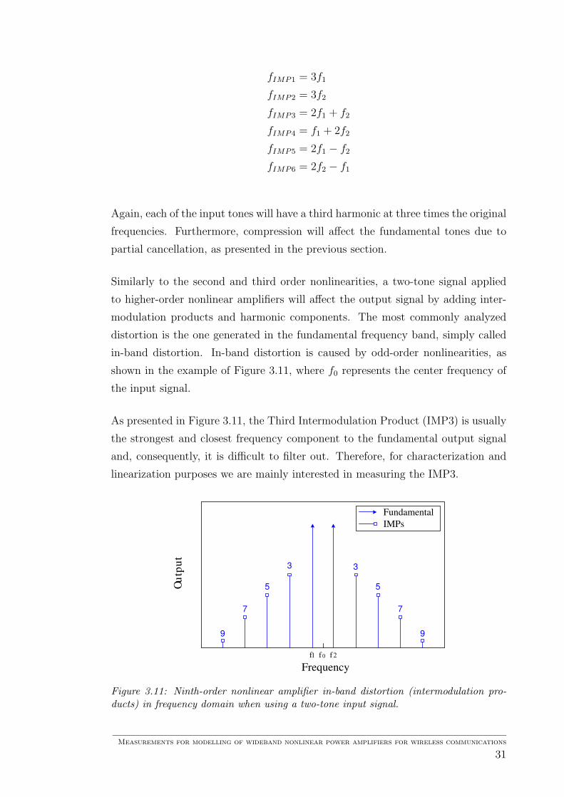
fIMP1 = 3f1
fIMP2 = 3f2
fIMP3 = 2f1 + f2
fIMP4 = f1 + 2f2
fIMP5 = 2f1 − f2
fIMP6 = 2f2 − f1
Again, each of the input tones will have a third harmonic at three times the original
frequencies. Furthermore, compression will affect the fundamental tones due to
partial cancellation, as presented in the previous section.
Similarly to the second and third order nonlinearities, a two-tone signal applied
to higher-order nonlinear amplifiers will affect the output signal by adding inter-
modulation products and harmonic components. The most commonly analyzed
distortion is the one generated in the fundamental frequency band, simply called
in-band distortion. In-band distortion is caused by odd-order nonlinearities, as
shown in the example of Figure 3.11, where f0 represents the center frequency of
the input signal.
As presented in Figure 3.11, the Third Intermodulation Product (IMP3) is usually
the strongest and closest frequency component to the fundamental output signal
and, consequently, it is difficult to filter out. Therefore, for characterization and
linearization purposes we are mainly interested in measuring the IMP3.
Frequency
f 1
3 3
5 5
7 7
f 2
9 9
f 0
Fundamental
IMPs
O u t p
u t
Figure 3.11: Ninth-order nonlinear amplifier in-band distortion (intermodulation pro-ducts) in frequency domain when using a two-tone input signal.
Measurements for modelling of wideband nonlinear power amplifiers for wireless communications
31
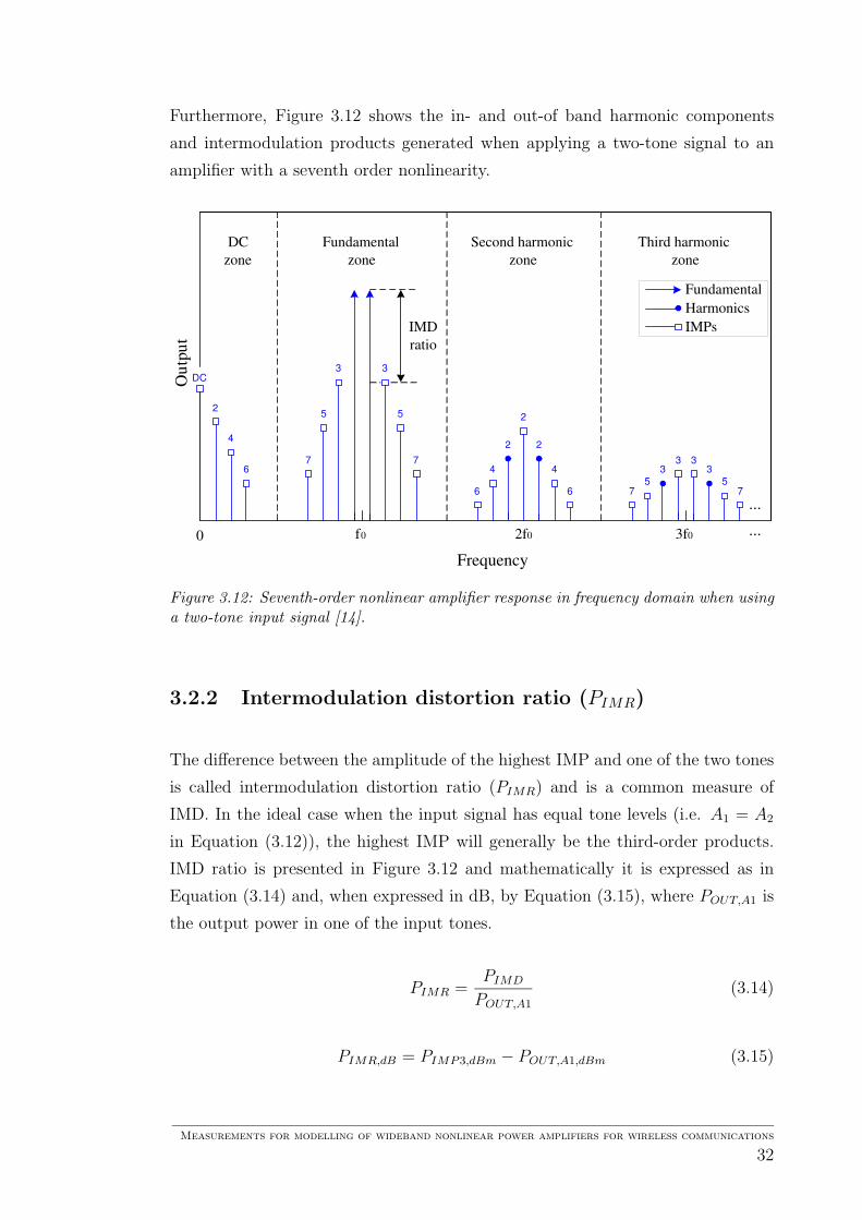
Furthermore, Figure 3.12 shows the in- and out-of band harmonic components
and intermodulation products generated when applying a two-tone signal to an
amplifier with a seventh order nonlinearity.
Frequency
0 2f 0 3f 0 f 0
Fundamental
Harmonics
IMPs
Fundamental
zone
Second harmonic
zone
Third harmonic
zone
DC
zone
...
...
DC
2 2
2 2
3 3
3 3 3 3
4
4 4
5 5
5 5
6
6 6
7 7
7 7
IMD
ratio
O u
t p u t
Figure 3.12: Seventh-order nonlinear amplifier response in frequency domain when usinga two-tone input signal [14].
3.2.2 Intermodulation distortion ratio (PIMR)
The difference between the amplitude of the highest IMP and one of the two tones
is called intermodulation distortion ratio (PIMR) and is a common measure of
IMD. In the ideal case when the input signal has equal tone levels (i.e. A1 = A2
in Equation (3.12)), the highest IMP will generally be the third-order products.
IMD ratio is presented in Figure 3.12 and mathematically it is expressed as in
Equation (3.14) and, when expressed in dB, by Equation (3.15), where POUT,A1 is
the output power in one of the input tones.
PIMR =PIMD
POUT,A1
(3.14)
PIMR,dB = PIMP3,dBm − POUT,A1,dBm (3.15)
Measurements for modelling of wideband nonlinear power amplifiers for wireless communications
32

3.2.3 IMD and Carrier-to-Noise Ratio (CNR)
When noise is present in a system affected by IMD, the Carrier-to-Noise Ratio
(CNR) will be degraded according to Equation (3.16), where CNRI is the CNR
caused only by the system noise and CID is the difference between the Carrier-
to-Interference Ratio (CIR) and the intrinsic CNR. The referred “intrinsic” noise
is the noise generated by the system itself, without including any IMD, which is
usually negative, implying that the system noise is higher than the one caused by
the IMD.
CNRN&IMD = CNRI − 10 log(
1 + 10CID/10)
(3.16)
For measurement purposes, noise is not included in the system (except the un-
avoidable intrinsic system noise). Therefore, CNR will not be calculated in this
research. However, CNR is a good measure of distortion when noisy signals are
applied to a system.
3.2.4 Spurious signals
Signals different than the fundamental tones, harmonic components and IMPs
may appear at the output of an amplifier, which are called spurious signals. These
signals may not keep any obvious relationship with the signals being amplified and
may appear, disappear, move between frequencies and change level randomly.
Spurious signals consist on low-level Radio Frequency (RF) oscillations, as well as
external interference caused by the high proximity of other devices in the same
system. This is one of the main reasons to search for extremely stable and robust
amplifiers for wireless communications.
Measurements for modelling of wideband nonlinear power amplifiers for wireless communications
33

3.3 Distortion measures using multi-tone signals
The earlier presented two-tone signal gives a good indication of the degree of dis-
tortion present in an amplifier when operating it with simple signals. However,
most modern systems are based on more complex signals and therefore, other mea-
surements are required. For example, Orthogonal Frequency Division Multiplexing
(OFDM) signals are a special type of multi-tone signals, which have become very
popular in modern communications due to its immunity to multipath fading chan-
nels [16].
In an OFDM transmission, the channel bandwidth is split into multiple parallel
transmissions or subcarriers. In the frequency domain, the subcarriers overlap
with each other, which is the main difference with the simple Frequency Divi-
sion Multiplexing (FDM) method [18]. Moreover, the signals transmitted in these
subcarriers are orthogonal with each other, which means that they can be clearly
separated without causing any crosstalk. The spectrum of an OFDM signal with
four subcarriers (fc) is illustrated in Figure 3.13, where the overlapping and the
orthogonality of the signals can be easily appreciated.
fc1 fc2 fc3 fc4
Frequency
Am
plitu
de
Figure 3.13: Orthogonal frequency division multiplexing signalling in frequency domain.
In this thesis, a multisine signal was chosen as test signal to perform multi-tone
measurements, since it is the simplest example of a high Peak-to-Average Ratio
(PAR) signal. When the bias of the amplifier is set near to the saturation zone,
Measurements for modelling of wideband nonlinear power amplifiers for wireless communications
34
the high peaks of the multisine signal are clipped at the output of the amplifier. It
is possible to avoid this by setting the bias of the amplifier at a lower input level,
which will result in a lower output power level. Operating the amplifier at a low
bias means that it is operated at a low efficiency rate. Therefore, the problem of
amplifier nonlinearity has a major effect on signals with high PAR, such as the
chosen multisine signal or the more complex OFDM signal [19]. A more detailed
PAR analysis in multicarrier transmission systems can be found in [20].
The chosen multisine signal (Ms(t)) consist of several simultaneously generated
sinewaves, with constant frequency spacing, random phase (Φ) and amplitude (A)
[21] and defined by Equation 3.17, where n is a positive integer and fb is the
basic frequency. Furthermore, the way of producing a practical multisine signal
for measurement purposes is analyzed in Section 5.2.4.
Ms(t) =N
∑
k=1
Ak cos(2πnkfbt + Φk) (3.17)
Multisine signals are a good approximation of modulated excitations and, there-
fore, they are widely used to test RF amplifiers. Using multisine signals instead of
modulated ones for multi-tone measurements has advantages such as having good
control of PAR characteristic and being easier to generate.
In general, multisine signals can be used for diverse purposes such as assessing the
intermodulation distortion of RF components [22], modelling the behavior of RF
circuits with short-memory effects [23] and modelling amplifiers with the Wiener-
Hammerstein model [24, 25]. Moreover, special types of multisine signals can be
generated for specific applications. For instance, odd-odd multisine signals, which
are used as a simple test to measure the best linear approximation [26], minimum
crest factor multisine signals for fast nonlinear system recognition [27] and paired
multisine signals for identification of nonlinear cascade systems [28].
For any kind of multi-tone signals (e.g. multisine and OFDM signals) some stan-
dard measurements have been defined in order to determine the degree of unwanted
signal energy caused by the nonlinearity of an amplifier. Next, these multi-tone
nonlinearity measures are presented.
Measurements for modelling of wideband nonlinear power amplifiers for wireless communications
35
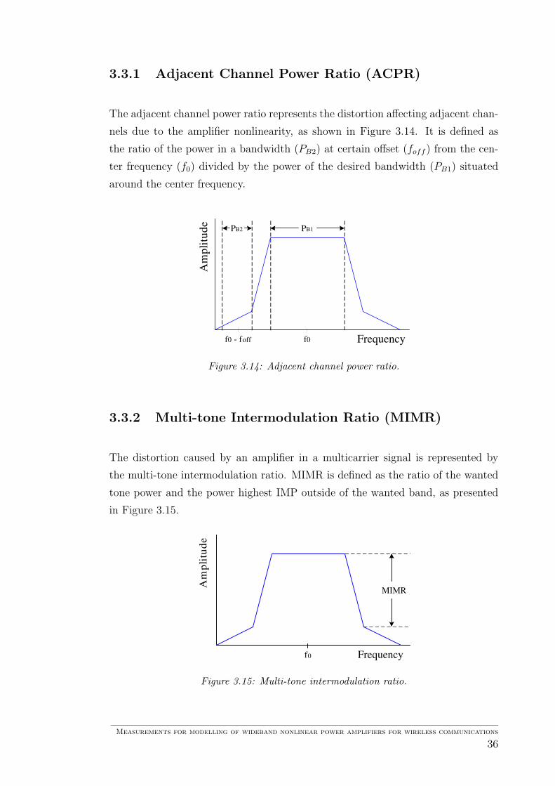
3.3.1 Adjacent Channel Power Ratio (ACPR)
The adjacent channel power ratio represents the distortion affecting adjacent chan-
nels due to the amplifier nonlinearity, as shown in Figure 3.14. It is defined as
the ratio of the power in a bandwidth (PB2) at certain offset (foff ) from the cen-
ter frequency (f0) divided by the power of the desired bandwidth (PB1) situated
around the center frequency.
Frequency
A m
p l i
t u d
e
f 0 - f off
P B2
f 0
P B1
Figure 3.14: Adjacent channel power ratio.
3.3.2 Multi-tone Intermodulation Ratio (MIMR)
The distortion caused by an amplifier in a multicarrier signal is represented by
the multi-tone intermodulation ratio. MIMR is defined as the ratio of the wanted
tone power and the power highest IMP outside of the wanted band, as presented
in Figure 3.15.
Frequency
A m
p l i
t u d
e
f 0
MIMR
Figure 3.15: Multi-tone intermodulation ratio.
Measurements for modelling of wideband nonlinear power amplifiers for wireless communications
36
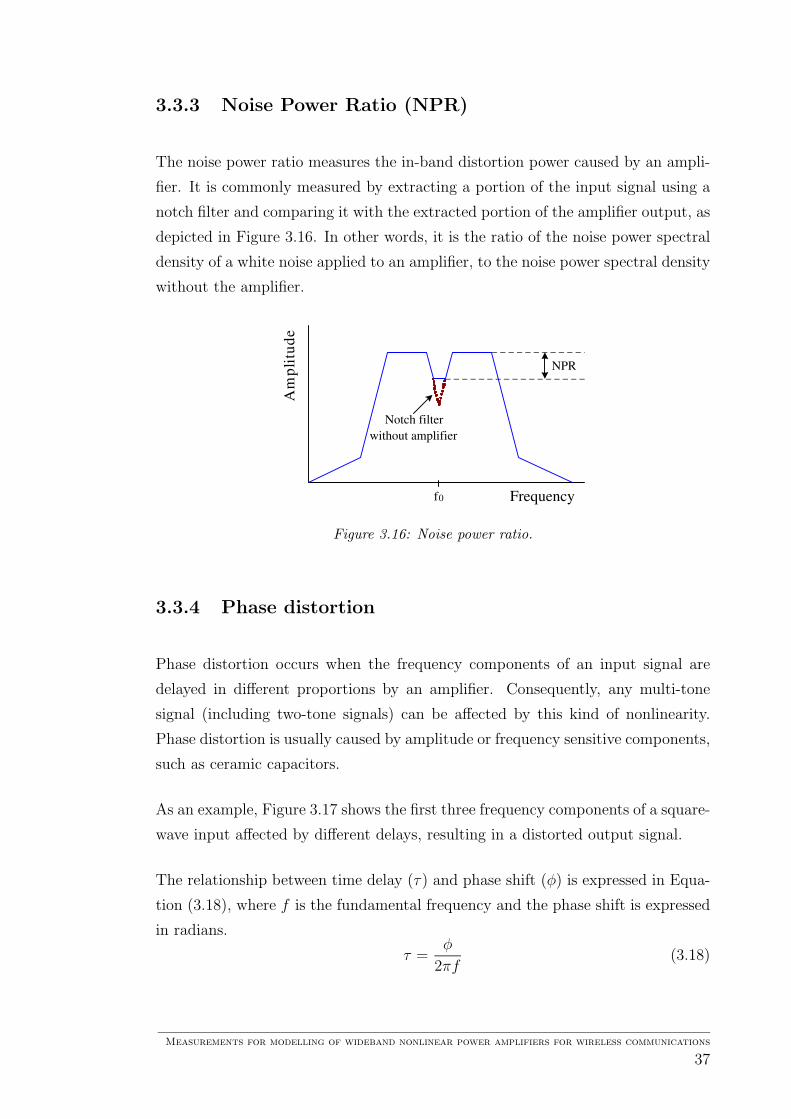
3.3.3 Noise Power Ratio (NPR)
The noise power ratio measures the in-band distortion power caused by an ampli-
fier. It is commonly measured by extracting a portion of the input signal using a
notch filter and comparing it with the extracted portion of the amplifier output, as
depicted in Figure 3.16. In other words, it is the ratio of the noise power spectral
density of a white noise applied to an amplifier, to the noise power spectral density
without the amplifier.
Frequency
A m
p l i
t u d
e
f 0
NPR
Notch filter
without amplifier
Figure 3.16: Noise power ratio.
3.3.4 Phase distortion
Phase distortion occurs when the frequency components of an input signal are
delayed in different proportions by an amplifier. Consequently, any multi-tone
signal (including two-tone signals) can be affected by this kind of nonlinearity.
Phase distortion is usually caused by amplitude or frequency sensitive components,
such as ceramic capacitors.
As an example, Figure 3.17 shows the first three frequency components of a square-
wave input affected by different delays, resulting in a distorted output signal.
The relationship between time delay (τ) and phase shift (φ) is expressed in Equa-
tion (3.18), where f is the fundamental frequency and the phase shift is expressed
in radians.
τ =φ
2πf(3.18)
Measurements for modelling of wideband nonlinear power amplifiers for wireless communications
37

Note that if the phase shift increases proportionally to the frequency, the time delay
will be the same for all frequency components. Therefore, in order to eliminate
phase distortion of the output signal of an amplifier, the delay should be constant,
which corresponds to linear phase.
0 0.0005 0.001 −2
−1
0
1
2
Resultant
Inpu
t
0 0.0005 0.001 −2
−1
0
1
2
Resultant
Out
put
0 0.0005 0.001 −2
−1
0
1
2
Fundamental
Inpu
t
0 0.0005 0.001 −2
−1
0
1
2
Fundamental
Out
put
0 0.0005 0.001 −2
−1
0
1
2
Third harmonic
Inpu
t
0 0.0005 0.001 −2
−1
0
1
2
Third harmonic
Out
put
0 0.0005 0.001 −2
−1
0
1
2
Fifth harmonic
Inpu
t
0 0.0005 0.001 −2
−1
0
1
2
Fifth harmonic
Out
put
Figure 3.17: Phase distortion in time domain of a 1 kHz squarewave (Input =sin(2πft)+0.6 sin(2π(3f)t)−0.3 sin(2π(5f)t)) applied to an amplifier with phase distor-tion, producing delays of 100 µs, 200 µs and 300 µs in the fundamental, third harmonicand fifth harmonic, respectively.
Measurements for modelling of wideband nonlinear power amplifiers for wireless communications
38
3.4 Summary of the chapter
The most common distortion parameters obtained from measurements using diffe-
rent signals applied to power amplifiers were summarized in this chapter. Harmonic
distortion appearing at frequencies multiple of the fundamental frequency is the
main nonlinear effect produced by single-tone input signals. Moreover, AM-AM
and AM-PM characteristic curves respectively show the output amplitude and
phase behavior when varying the input signal. However, it is necessary to perform
a frequency-sweep measurement, in order to represent the memory effects intro-
duced by amplifiers. Other parameters obtained using single-tone input signals are
the back-off, second- and third-order intercept points and the 1 dB compression
point. The two last of these are commonly used by manufacturers as indicators of
amplifiers’ linearity.
When measuring the linearity of an amplifier it is convenient to use a two-tone
input signal since, besides the harmonic distortion, intermodulation products will
be shown in the output spectrum. The third intermodulation product present in
the fundamental zone is the most important parameter obtained from a two-tone
test because it is the frequency component closest to the fundamental tone and,
therefore, it is difficult to filter out with simple methods.
A multisine signal was chosen in this research for measuring the effects of a non-
linear amplifier over high peak-to-average ratio signals. The characteristics of
multisine signals, as well an introduction to Orthogonal Frequency Division Mul-
tiplexing (OFDM) transmission scheme, were given. Finally, the most common
measures of nonlinearity obtained with multi-tone signals (adjacent channel power
ratio, multi-tone intermodulation ratio and noise power ratio) were summarized.
Measurements for modelling of wideband nonlinear power amplifiers for wireless communications
39

Chapter 4
Background for planning
measurements
Chapter 2 described the main characteristics of power amplifiers. Ideally, an am-
plifier should linearly increase the power applied to it. However, in practice, am-
plifiers behave in a nonlinear way, which usually causes unwanted distortion in the
output of the system where the amplifier is used. Measures of amplifier distortion
were presented in Chapter 3.
When the predominant distortion affecting an amplifier in a system is known, it
is possible to model the nonlinearity by using an adequate estimator. This means
that the data obtained from measurements of power amplifiers can be used to
characterize and, later on, alleviate the nonlinearity introduced by amplifiers to a
system.
This chapter provides a summary of theoretical background needed to determine
the type of measurements that will better characterize amplifier distortion. First,
an overview of methods for modelling nonlinear power amplifiers is given. Finally,
the theory necessary to estimate the parameters required to model amplifiers is
summarized.
Measurements for modelling of wideband nonlinear power amplifiers for wireless communications
40
4.1 Methods for modelling power amplifiers
Models that represent the nonlinearity of an amplifier can be accurately designed
based on measurement results, such as the ones introduced in Chapter 3. In
general, methods for modelling amplifiers can be classified according to the memory
characteristics of the amplifier into memoryless models and models with memory
[29].
Models for memoryless nonlinearities or Zero-Memory Nonlinearity (ZMNL) can
be subdivided into two approaches. The first of these is an analytical approach,
referred as memoryless baseband nonlinearity, which is based on an input sig-
nal whose power spectrum is concentrated around zero frequency. The second
approach is the memoryless bandpass nonlinearity, which is mainly an empirical
approach since it is characterized by measurements performed on the amplifier to
be modelled.
Memoryless models are an idealization of practical systems since no physical device
is truly frequency-independent, which is a requirement for a memoryless model.
Therefore, Nonlinearity with Memory (NLWM) models are a more accurate ap-
proach for nonlinear power amplifiers.
The most commonly used ZMNL and NLWM modelling methods [29] are summa-
rized in Figure 4.1, including references to each particular method.
An example of the application of the polynomial and Hammerstein models to
characterize the ZVE-8G amplifier [5] is described in Section 7.2. This model is
based on measurements performed as part of this research and is introduced in
this thesis as a way or proving the usefulness of amplifier measurements.
Measurements for modelling of wideband nonlinear power amplifiers for wireless communications
41
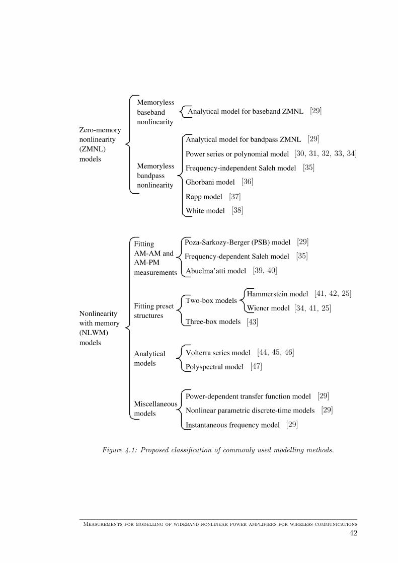
Zero-memory
nonlinearity
(ZMNL)
models
Nonlinearity
with memory
(NLWM)
models
Memoryless
baseband
nonlinearity
Memoryless
bandpass
nonlinearity
Analytical model for baseband ZMNL
Analytical model for bandpass ZMNL
Power series or polynomial model
Frequency-independent Saleh model
Ghorbani model
Rapp model
White model
Fitting
AM-AM and
AM-PM
measurements
Poza-Sarkozy-Berger (PSB) model
Frequency-dependent Saleh model
Abuelma’atti model
Fitting preset
structures
Two-box models
Three-box models
Analytical
models
Volterra series model
Polyspectral model
Miscellaneous
models
Power-dependent transfer function model
Nonlinear parametric discrete-time models
Instantaneous frequency model
Hammerstein model
Wiener model
[29]
[29]
[29]
[29]
[29]
[29]
[30, 31, 32, 33, 34]
[35]
[35]
[36]
[37]
[38]
[39, 40]
[41, 42, 25]
[34, 41, 25]
[43]
[44, 45, 46]
[47]
Figure 4.1: Proposed classification of commonly used modelling methods.
Measurements for modelling of wideband nonlinear power amplifiers for wireless communications
42
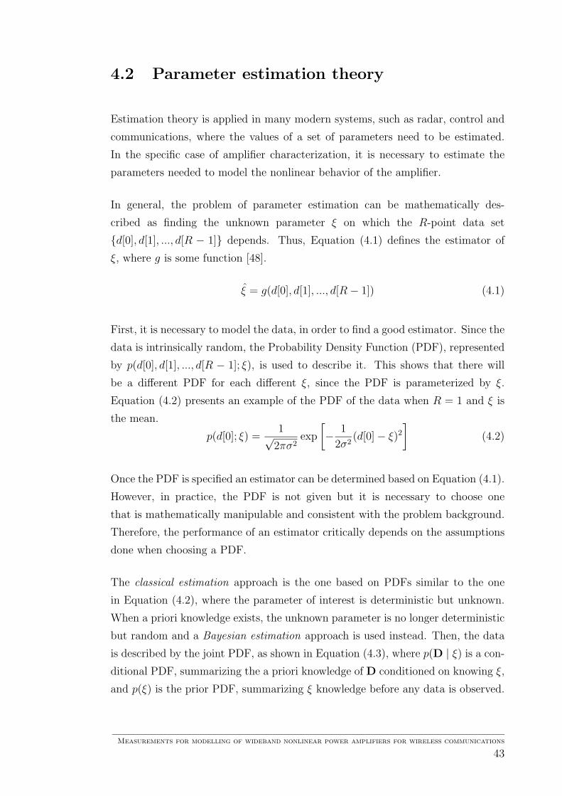
4.2 Parameter estimation theory
Estimation theory is applied in many modern systems, such as radar, control and
communications, where the values of a set of parameters need to be estimated.
In the specific case of amplifier characterization, it is necessary to estimate the
parameters needed to model the nonlinear behavior of the amplifier.
In general, the problem of parameter estimation can be mathematically des-
cribed as finding the unknown parameter ξ on which the R-point data set
d[0], d[1], ..., d[R − 1] depends. Thus, Equation (4.1) defines the estimator of
ξ, where g is some function [48].
ξ = g(d[0], d[1], ..., d[R − 1]) (4.1)
First, it is necessary to model the data, in order to find a good estimator. Since the
data is intrinsically random, the Probability Density Function (PDF), represented
by p(d[0], d[1], ..., d[R − 1]; ξ), is used to describe it. This shows that there will
be a different PDF for each different ξ, since the PDF is parameterized by ξ.
Equation (4.2) presents an example of the PDF of the data when R = 1 and ξ is
the mean.
p(d[0]; ξ) =1√
2πσ2exp
[
− 1
2σ2(d[0] − ξ)2
]
(4.2)
Once the PDF is specified an estimator can be determined based on Equation (4.1).
However, in practice, the PDF is not given but it is necessary to choose one
that is mathematically manipulable and consistent with the problem background.
Therefore, the performance of an estimator critically depends on the assumptions
done when choosing a PDF.
The classical estimation approach is the one based on PDFs similar to the one
in Equation (4.2), where the parameter of interest is deterministic but unknown.
When a priori knowledge exists, the unknown parameter is no longer deterministic
but random and a Bayesian estimation approach is used instead. Then, the data
is described by the joint PDF, as shown in Equation (4.3), where p(D | ξ) is a con-
ditional PDF, summarizing the a priori knowledge of D conditioned on knowing ξ,
and p(ξ) is the prior PDF, summarizing ξ knowledge before any data is observed.
Measurements for modelling of wideband nonlinear power amplifiers for wireless communications
43
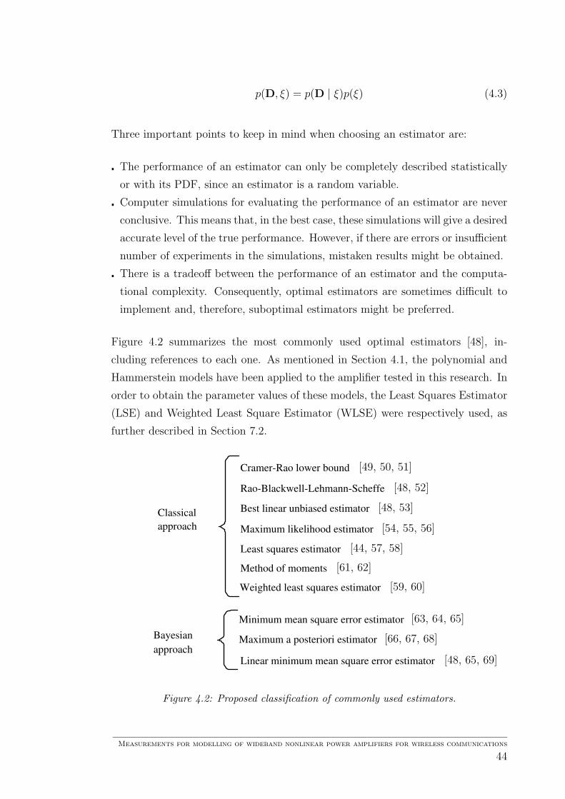
p(D, ξ) = p(D | ξ)p(ξ) (4.3)
Three important points to keep in mind when choosing an estimator are:
¦ The performance of an estimator can only be completely described statistically
or with its PDF, since an estimator is a random variable.
¦ Computer simulations for evaluating the performance of an estimator are never
conclusive. This means that, in the best case, these simulations will give a desired
accurate level of the true performance. However, if there are errors or insufficient
number of experiments in the simulations, mistaken results might be obtained.
¦ There is a tradeoff between the performance of an estimator and the computa-
tional complexity. Consequently, optimal estimators are sometimes difficult to
implement and, therefore, suboptimal estimators might be preferred.
Figure 4.2 summarizes the most commonly used optimal estimators [48], in-
cluding references to each one. As mentioned in Section 4.1, the polynomial and
Hammerstein models have been applied to the amplifier tested in this research. In
order to obtain the parameter values of these models, the Least Squares Estimator
(LSE) and Weighted Least Square Estimator (WLSE) were respectively used, as
further described in Section 7.2.
Classical
approach
Cramer-Rao lower bound
Rao-Blackwell-Lehmann-Scheffe
Best linear unbiased estimator
Maximum likelihood estimator
Least squares estimator
Method of moments
Bayesian
approach
Minimum mean square error estimator
Maximum a posteriori estimator
Linear minimum mean square error estimator
Weighted least squares estimator
[49, 50, 51]
[48, 52]
[48, 53]
[54, 55, 56]
[44, 57, 58]
[59, 60]
[61, 62]
[63, 64, 65]
[66, 67, 68]
[48, 65, 69]
Figure 4.2: Proposed classification of commonly used estimators.
Measurements for modelling of wideband nonlinear power amplifiers for wireless communications
44
4.3 Summary of the chapter
Processing of the data obtained from the measurements performed in this thesis
in order to alleviate amplifier distortion was discussed in this chapter. First, a
brief overview of methods to model power amplifiers was done, including some
references for more information. Moreover, the measurements performed in this
research can be used in some of these methods, such as the Hammerstein model
applied to the amplifier tested in this thesis [5].
Next, parameter estimation concepts useful when modelling amplifier nonlinearity
were introduced. Classical and Bayesian estimation approaches were defined by the
Probability Density Function (PDF) and the joint PDF, respectively. Furthermore,
the most commonly used estimators were summarized and references of each were
given.
The concepts covered in this chapter will not be practically applied in this thesis
since the objective of the research is mainly to obtain the necessary parameters to
model power amplifiers by performing different types of measurements. However,
this theory gives a good background that is helpful when planning the type of
amplifier measurements to be performed. Nevertheless, an example of the imple-
mentation of the results obtained in this thesis on modelling an amplifier can be
found in [5] and will be briefly covered in Section 7.2.
Measurements for modelling of wideband nonlinear power amplifiers for wireless communications
45
Chapter 5
Power amplifier measurement
planning
The previous chapters have covered the basic concepts about amplifier distortion.
As mentioned in Chapter 3, memoryless distortion can be represented by parame-
ters obtained from single-tone measurements, such as the AM-AM and AM-PM
characteristics, which respectively show how the amplitude and phase of the output
changes when varying the input power level. However, for systems with memory
or when using non-constant envelope modulated input signals, it is preferable to
perform a two-tone transfer characteristics measurement. Furthermore, for sys-
tems using more complex signals (e.g. OFDM signals), multi-tone measurements
are recommended in order to characterize the amplifier as accurately as possible.
In this chapter, the basic knowledge required to perform amplifier measurements is
summarized. First, comments on the importance of careful and good planning are
given. Next, a brief description of the characteristics of the input testing signals,
the equipment used, calibration procedure and noise considerations is done. Fi-
nally, the way of performing different types of amplifier tests is described, including
the performance parameters, setup systems and processes for each measurement.
Measurements for modelling of wideband nonlinear power amplifiers for wireless communications
46

5.1 Before measurements
When making measurements of any kind of device, the most important is to test
them “correctly”. There are many factors involved in the correct testing of devices
because, opposite to simulating environment, in practice there are not perfect
systems.
Errors introduced for example by connector mismatches or cable losses can change
the results but can be minimized by careful planning. Other areas where problems
can occur are briefly described next [70]:
¦ Analyzing beforehand which parameters will best characterize the Device Under
Test (DUT) and then, test only these will save time by avoiding doing unneces-
sary measurements. Moreover, the most important information of the DUT will
be obtained.
¦ In order to have correctly done measurements, it is necessary to have the proper
equipment, put it in the right order and know how to operate it. In other words,
it is useful to have a setup system proper to test the wanted parameters.
¦ The procedure to perform measurements should be carefully planed and ana-
lyzed in order to find the possible errors, losses and power levels needed that
may affect the results. Therefore, it is important to know how to perform the
desired measurement.
¦ It is always convenient to get the parameters to be measured displayed in the
screen. However, in some cases it might be needed to make some calculations
in order to obtain the desired data. A proper understanding of the measuring
equipment capabilities will save time and make easier to get the correct data.
The four points covered are meant to emphasize the importance of beforehand
careful planning, which might save time and will give not just results but “correct”
results.
Measurements for modelling of wideband nonlinear power amplifiers for wireless communications
47

5.1.1 Choice of input signal
In the specific case of amplifier measurements for modelling purposes, an extra
point to those previously mentioned should be taken on count. This aspect consists
of choosing the adequate excitation (i.e. input signal) that allows the output data
to carry sufficient information on the parameters to be estimated.
Different input signals are used for different measures of amplifier nonlinearity.
Single-tone signals are used to perform power and frequency sweeps which will
give as result the input-output curves from which the 1 dB Compression Point
(1 dB CP) can be extracted. Moreover, harmonic distortion can be easily obtained
by using this kind of simple signals. On the other hand, two-tone signals are used to
characterize the intermodulation distortion produced by amplifiers. However, the
phase relationship and frequency separation of the tones composing signals with
more than two tones will affect the Peak-to-Average Ratio (PAR). Consequently,
multi-tone signals will enable to test the worst PAR cases. Furthermore, the more
tones are used in the input signal, the best approximation of modulated signals
response is obtained [71].
A one-sinusoid signal used to measure amplifier nonlinearity has the main advan-
tage of simplicity and, consequently, the results obtained are easy to interpret
[72]. The measuring dynamic and frequency ranges constitute the most important
factors for single-tone input signal measurements. The dynamic range used for
power-sweep measurements should cover a part of the linear zone and the nonli-
near zone (i.e. from a low input level to some decibels above the 1 dB CP). On the
other hand, the range for frequency-sweep measurements should be enough wide
to cover the whole operating frequency range of the amplifier.
AM-AM and AM-PM characteristics obtained from single-tone measurements are
static measurements, which may include thermal or DC bias effects. In the wireless
communications environment this distortion occurs dynamically, since the ampli-
tude envelope of the signals can vary according to the information rate. Therefore,
amplitude and phase distortion are dynamically characterized by measuring the
intermodulation distortion using a two-tone signal [43]. The separation of the in-
put tones should be chosen according to the intermodulation product’s maximum
order to be analyzed. However, this depends on the maximum sampling frequency
Measurements for modelling of wideband nonlinear power amplifiers for wireless communications
48

of the generator used (i.e. AWG), as it is further explained in Section 5.2.3. More-
over, the input level used to measure the distortion introduced by the amplifier
should be as close as possible to the 1 dB CP and the frequency of the two tones
should fall inside the amplifier’s operating frequency range.
Finally, multi-tone signals are widely used to analyze the distortion introduced by
amplifiers, since they provide a good approximation to the response obtained with
complex modulated signals (e.g. OFDM). For instance, it is proven that multisine
input signals with constant amplitude and random phase spectrum are the most
appropriate to accurately model the behavior of nonlinear power amplifiers [73].
Ideally, the input signal should cover the whole frequency band for which the model
is desired. In some cases, the equipment availability might limit this range and,
therefore, the maximum possible bandwidth should be used. Once more, the input
level should be chosen as close to the 1 dB CP as possible, in order to obtained a
good measure of the nonlinear characteristic of the amplifier.
5.1.2 Equipment
In this section, a brief description of the working of the devices used for amplifier
measurements is given, including signal generators, signal detection devices, auxi-
liary components and DUTs. For each of these categories, specific devices were
chosen in order to fully test the characteristics of the DUT and so, their main
parameters are also given, in order to help in the design of test systems and in the
planning and interpretation of results done in the following chapters.
Vector Signal Generator
A Signal Generator (SG) gives an AC signal of variable amplitude and variable
frequency to be used when operating an amplifier or other circuit. Usually, fre-
quency may be varied from a few hertz to some megahertz or even gigahertz. The
amplitude can be adjusted from a few millivolts up to some volts and these values
can be also adjusted in millidecibels form. In addition to sinusoidal signals, other
commonly used waveforms, such as square or triangular, can be produced with
this equipment.
Measurements for modelling of wideband nonlinear power amplifiers for wireless communications
49
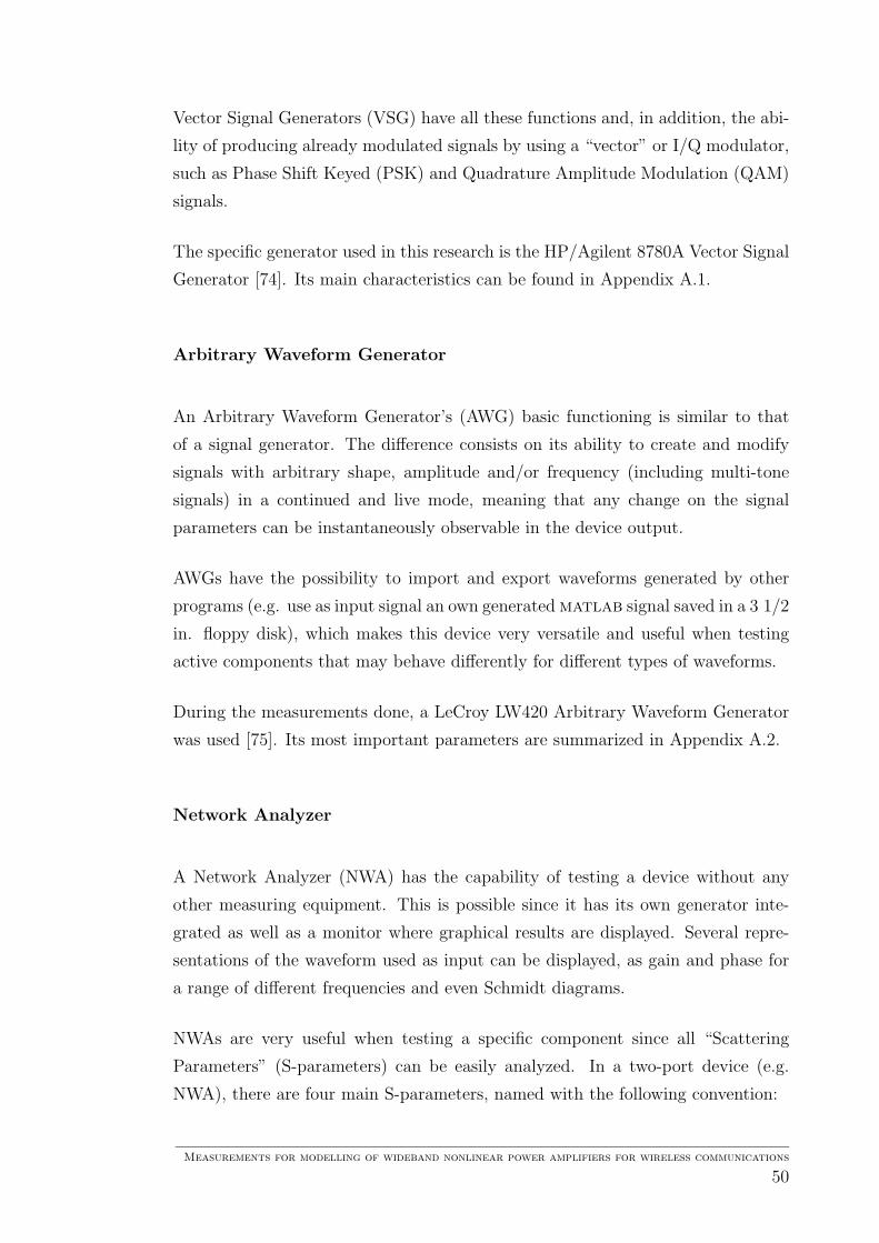
Vector Signal Generators (VSG) have all these functions and, in addition, the abi-
lity of producing already modulated signals by using a “vector” or I/Q modulator,
such as Phase Shift Keyed (PSK) and Quadrature Amplitude Modulation (QAM)
signals.
The specific generator used in this research is the HP/Agilent 8780A Vector Signal
Generator [74]. Its main characteristics can be found in Appendix A.1.
Arbitrary Waveform Generator
An Arbitrary Waveform Generator’s (AWG) basic functioning is similar to that
of a signal generator. The difference consists on its ability to create and modify
signals with arbitrary shape, amplitude and/or frequency (including multi-tone
signals) in a continued and live mode, meaning that any change on the signal
parameters can be instantaneously observable in the device output.
AWGs have the possibility to import and export waveforms generated by other
programs (e.g. use as input signal an own generated matlab signal saved in a 3 1/2
in. floppy disk), which makes this device very versatile and useful when testing
active components that may behave differently for different types of waveforms.
During the measurements done, a LeCroy LW420 Arbitrary Waveform Generator
was used [75]. Its most important parameters are summarized in Appendix A.2.
Network Analyzer
A Network Analyzer (NWA) has the capability of testing a device without any
other measuring equipment. This is possible since it has its own generator inte-
grated as well as a monitor where graphical results are displayed. Several repre-
sentations of the waveform used as input can be displayed, as gain and phase for
a range of different frequencies and even Schmidt diagrams.
NWAs are very useful when testing a specific component since all “Scattering
Parameters” (S-parameters) can be easily analyzed. In a two-port device (e.g.
NWA), there are four main S-parameters, named with the following convention:
Measurements for modelling of wideband nonlinear power amplifiers for wireless communications
50
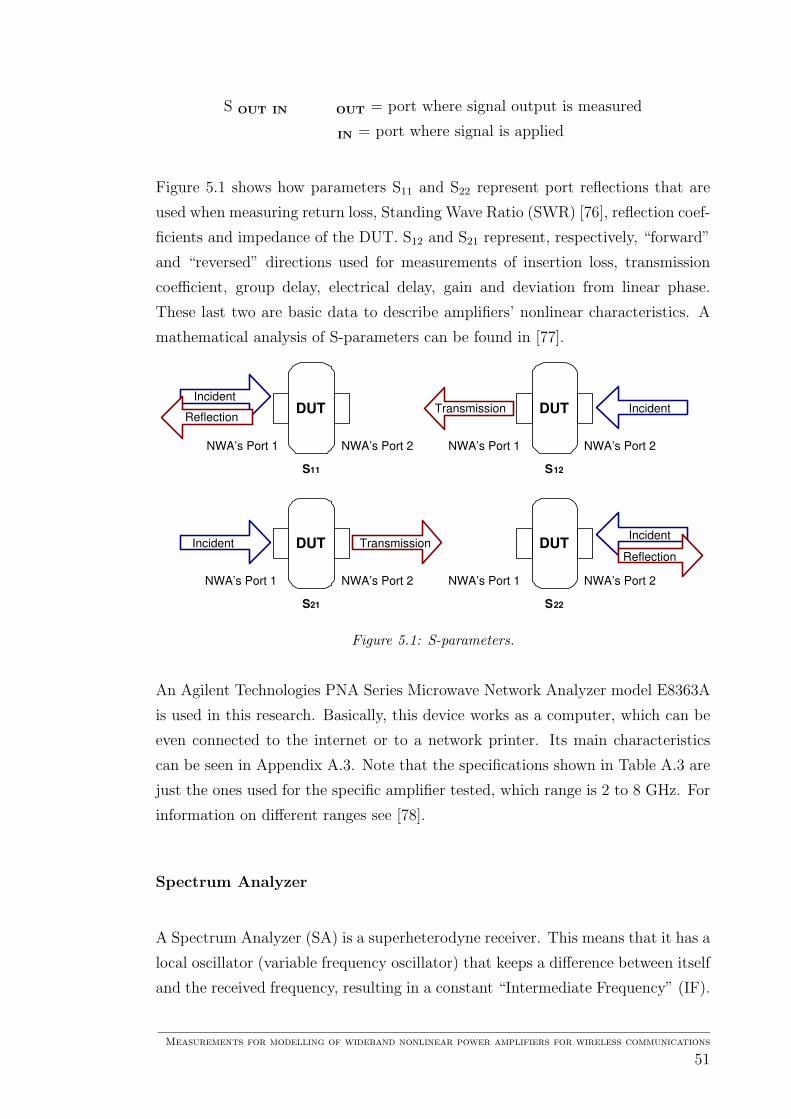
S OUT IN OUT = port where signal output is measured
IN = port where signal is applied
Figure 5.1 shows how parameters S11 and S22 represent port reflections that are
used when measuring return loss, Standing Wave Ratio (SWR) [76], reflection coef-
ficients and impedance of the DUT. S12 and S21 represent, respectively, “forward”
and “reversed” directions used for measurements of insertion loss, transmission
coefficient, group delay, electrical delay, gain and deviation from linear phase.
These last two are basic data to describe amplifiers’ nonlinear characteristics. A
mathematical analysis of S-parameters can be found in [77].
DUT Incident Transmission DUT
NWA’s Port 1
Incident
Reflection
DUT Incident
Reflection DUT Incident Transmission
S 11 S 12
S 21 S 22
NWA’s Port 1
NWA’s Port 1
NWA’s Port 1
NWA’s Port 2
NWA’s Port 2
NWA’s Port 2
NWA’s Port 2
Figure 5.1: S-parameters.
An Agilent Technologies PNA Series Microwave Network Analyzer model E8363A
is used in this research. Basically, this device works as a computer, which can be
even connected to the internet or to a network printer. Its main characteristics
can be seen in Appendix A.3. Note that the specifications shown in Table A.3 are
just the ones used for the specific amplifier tested, which range is 2 to 8 GHz. For
information on different ranges see [78].
Spectrum Analyzer
A Spectrum Analyzer (SA) is a superheterodyne receiver. This means that it has a
local oscillator (variable frequency oscillator) that keeps a difference between itself
and the received frequency, resulting in a constant “Intermediate Frequency” (IF).
Measurements for modelling of wideband nonlinear power amplifiers for wireless communications
51

Its main purpose is to receive a range of signals and display their frequency com-
ponents in a graphic form. The procedure to do this is based on the relationship
between time and frequency domains that can be mathematically analyzed via
Fourier transforms.
In a SA, the convolution of a very narrow band-pass filter (ideally an impulse)
and the received signal is done, resulting in the frequency domain characteristics
(spectrum) of the signal. The filter mentioned is a critical part in this kind of
sweeping devices. It is called ”resolution filter” and is, in fact, the bandwidth of
the intermediate frequency.
In the specific case of amplifier measurements it is very important to analyze the
spectrum of its output since different types of distortions may appear on it, as
explained on Chapter 3. Other parameters that can be obtained with this device
are power, frequency, noise, sensitivity and modulation.
The spectrum analyzer used in this specific measurements is an Agilent Technolo-
gies 8564EC. Its more important specifications for the range of the amplifier used
are shown in Appendix A.4. The complete data sheet can be found in [79].
Active Components
Components to be measured can be classified as passive and active. The first
ones are the devices that do not affect their resistance, impedance or reactance
when alternating currents are applied to them. This means that they will consume
energy (change energy into other forms than electrical, as heat or light) or store
it (as in electromagnetic fields). Examples of these devices are resistors, inductors
and capacitors [80]. Passive elements will not be explained in more detail since
they are linear devices.
An active component is “1. a component which adds energy to the signal it passes;
2. a device that requires an external source of power to operate upon its input
signal(s); 3. any device that switches or amplifies by the application of low-level
signals” [81]. In other words and for the purpose of this thesis, active compo-
nents are the ones that when an AC signal is applied to them their impedance or
resistance will change, and so, they will amplify, rectify, modify or distort these
Measurements for modelling of wideband nonlinear power amplifiers for wireless communications
52
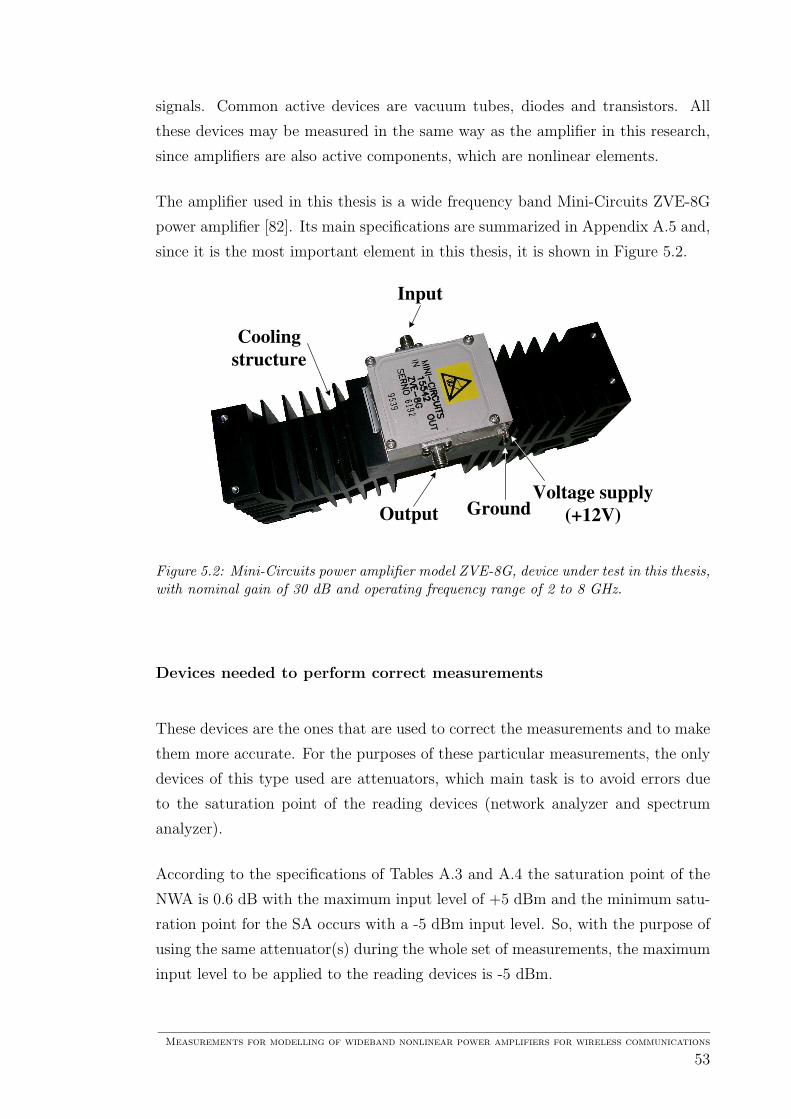
signals. Common active devices are vacuum tubes, diodes and transistors. All
these devices may be measured in the same way as the amplifier in this research,
since amplifiers are also active components, which are nonlinear elements.
The amplifier used in this thesis is a wide frequency band Mini-Circuits ZVE-8G
power amplifier [82]. Its main specifications are summarized in Appendix A.5 and,
since it is the most important element in this thesis, it is shown in Figure 5.2.
Input
Output
Voltage supply
(+12V) Ground
Cooling
structure
Figure 5.2: Mini-Circuits power amplifier model ZVE-8G, device under test in this thesis,with nominal gain of 30 dB and operating frequency range of 2 to 8 GHz.
Devices needed to perform correct measurements
These devices are the ones that are used to correct the measurements and to make
them more accurate. For the purposes of these particular measurements, the only
devices of this type used are attenuators, which main task is to avoid errors due
to the saturation point of the reading devices (network analyzer and spectrum
analyzer).
According to the specifications of Tables A.3 and A.4 the saturation point of the
NWA is 0.6 dB with the maximum input level of +5 dBm and the minimum satu-
ration point for the SA occurs with a -5 dBm input level. So, with the purpose of
using the same attenuator(s) during the whole set of measurements, the maximum
input level to be applied to the reading devices is -5 dBm.
Measurements for modelling of wideband nonlinear power amplifiers for wireless communications
53
Based on this and for the amplifier used we have the system shown in Figure 5.3
from which we derive the minimum needed attenuation (Att) equal to 38 dB (with a
maximum input power level of +3 dBm to the amplifier). The attenuation used for
the measurements in this thesis is 40 dB, due to the availability of equipment at the
measuring laboratory. This attenuation is obtained with 10 dB and 30 dB Midwest
Microwave attenuators, which main characteristics are shown in Appendix A.6.
Amp. Attenuator Reading
Device
Signal
Generator
+3 dBm (max.) +30 dB - Att = -5 dBm (max.)
Figure 5.3: System for calculation of attenuation needed for correct measurements.
The maximum input level to the amplifier was calculated based on the attenuators’
power specification, which is 2 W. This means that the maximum power applied to
them, and so the maximum output power from the amplifier, should be +33 dBm.
Then, the maximum input level applied to the input of the amplifier should not
be greater than +3 dBm.
With this input level defined, we make sure that the saturation zone of the amplifier
will be tested. According to Table A.5, 1 dB compression point of the amplifier,
referenced to the output power, is +30 dBm. Therefore, the saturation zone of
the amplifier begins at +1 dBm of input level, making the maximum input level
(+3 dBm) enough to measure the whole characteristics of the amplifier.
5.1.3 Calibration
There are two types of calibration: instrument calibration and measurement cali-
bration [83]. Every instrument was built to function in a specific way and so, it
was set up (calibrated) to accomplish its tasks in a proper way. However, aging,
temperature, usage and other factors can vary the equipments’ original values and
some adjustments might be necessary for their optimum operation. This is the
called instrument calibration and it is usually done by a technician of the instru-
ment manufacturer company, who ensures that the device is working within the
specifications.
Measurements for modelling of wideband nonlinear power amplifiers for wireless communications
54

On the other hand, measurement calibration corrects systematic errors using an
equation called error model. The systematic errors are the ones caused by imper-
fections in the equipment (e.g. adapter interface or interconnecting cables) and
test setup. They are predictable, can be calculated and can be mathematically
reduced but never totally removed due to limitations in the calibration process.
The amplitude at the DUT input and the frequency response accuracy are some of
the most important parameters that may be affected with an uncalibrated device.
Measurement calibration is recommended when:
¦ the best possible accuracy is desired
¦ adapting to a different connector type
¦ connecting cables in the system
¦ measuring through a wide frequency span
¦ connecting auxiliary devices in the input or output of the DUT
Each measuring device has its own calibration method(s) that should be performed
to assure that the obtained results are less affected by external factors to the DUT.
In the particular case of amplifier measurements, the calibration process of the
NWA and the SA will be discussed in more detail in Section 5.2.1.
5.1.4 Noise
In radio frequency and microwave measurements, the ultimate sensitivity of the
detector system is determined by the noise presented to the system and the noise
introduced by the system itself. This means that the weakest signal that a system
can detect depends on the amount of noise affecting it. This is why good knowledge
of the test equipment’s noise helps to make the results of measurements more
accurate.
Sources of noise can be external to the measurement system or within the system
itself. Electrical motors, dirty switch contacts and thunderstorms are examples
of external sources. Although these affect all systems, in radio or microwave fre-
quencies the internal sources are predominant and so, these are briefly explained
next.
Measurements for modelling of wideband nonlinear power amplifiers for wireless communications
55
Thermal noise, also called Johnson or Nyquist noise [84, 85], is the most important
internal type of noise because it is produced by any kind of component, active or
passive, and trends to be dominant in most systems. It refers to the electrical noise
that is produced with the random motion of electrons in a conductor due to heat
(without average current flowing through the conductor). The current between
two points, produced by the movement of electrons, generates a voltage. For RF
and microwave frequencies, this voltage has a uniform spectral distribution, which
makes this type of noise often called “white noise”. Since thermal noise affects ac-
tive and passive devices, any component in a system will affect the overall system
noise by generating “noise power”, which is defined as:
Pn = ZTB,
where Pn is the noise power in watts, T is the absolute temperature of the source,
B is the bandwidth of the system and Z is the Boltzmann constant (≈ 1.38 ×10⁻²³ J/K).
In addition to thermal noise, active devices produce other types of noise. A current
in a conductor, produced by random emanation of electrons, generates random
fluctuations called shot noise. In vacuum tubes, induced grid noise is produced as
a result of fluctuations in the electron stream passing adjacent to a grid. Partition
noise occurs in multi-electrode active devices, such as transistors and valves. When
the charge carriers in a current have the possibility of dividing between two or
more paths, the noise is generated in the resulting components of the current by
the statistical process of partition. Finally, Flicker noise, also called contact noise
or excess noise, is generated by the imperfect contact between two conducting
materials, which causes the conductivity to fluctuate in the presence of a DC
current.
Furthermore, the characteristic noise of an amplifier determines how well it per-
forms. The main noise parameters used to specify an amplifier performance [85]
are summarized next.
Noise temperature (Tn) Temperature in degrees Kelvin at which thermal noise
power is equal to the amount of available noise power (Pn) from the output of the
device.
Tn =Pn
Z= 7.25 × 10²²Pn
Measurements for modelling of wideband nonlinear power amplifiers for wireless communications
56

Noise ratio (rn) Ratio of the noise temperature to the actual temperature (Ta).
(The noise ratio minus unity is often called excess noise ratio)
rn =Tn
Ta
=Pn
ZTa
Noise factor (F) Ratio of the total available output noise power per unit band-
width to the portion caused by an input with a noise temperature of 290K.
F =Tn
290 + 1
Noise figure (Nf) Equivalent of the noise factor in dB, which can be also defined
as the ratio of the input Signal-to-Noise Ratio (SNR) to the output SNR.
Nf = 10 log F = 10 log
(
SNRinput
SNRoutput
)
Effective input noise temperature (Te) Temperature of the input at which
the available noise output power is twice that which would be available if the in-
put were at absolute zero. It determines an input temperature at which the input
thermal noise and the internal thermal noise from the device contribute equally to
the output noise.
Te = 290(F − 1)
Operating noise figure or noise sensitivity (τs) Ratio of available noise
power from the output when the input is at its normal operating temperature
(To) to the contribution which the input would make to the available output noise
power if it were at the standard temperature (290K).
τs = F − 1 +Ta
290
Noise measurements of the previous parameters are used mainly to compare the
performance of amplifiers. For the purpose of amplifier nonlinearity measurements,
the noise parameters proper to each specific amplifier do not give relevant infor-
mation. Therefore, noise measurements are not needed in this research and so,
they were not performed and analyzed. However, more information about noise
measurements can be found in [70] and [77].
Measurements for modelling of wideband nonlinear power amplifiers for wireless communications
57
5.2 Performing measurements
In this section, the performance parameters, setup systems (based on the equip-
ment introduced in Section 5.1.2) and the process to make different kind of ampli-
fier measurements are described. First, basic measurements of cables and loss due
to passive devices are explained. Next, single- and two-tone signal measurement
procedures are given. Finally, multi-tone signal testing using a multisine signal is
described.
5.2.1 Passive device measurements
When measuring amplifiers, passive devices are included in the setup system. In
this thesis, these devices are divided into devices needed to interconnect measu-
ring systems, such as cables and adapters, and devices needed to perform correct
measurements, which in this research consist only of attenuators, as explained in
Section 5.1.2.
Devices needed to interconnect measuring systems
Measurements of cables and adapters are done in order to obtain the loss intro-
duced by them. However, it is possible to avoid the effect of this loss in the mea-
surement results by calibrating the measuring equipment including all the cables
and adapters used during a particular test.
A THRU response calibration is the simplest that can be performed to NWAs and
to SAs including cables and adapters. The THRU response calibration is done by
measuring the system without connecting the DUT. In other words, the internal
generator of the measuring device is connected to the RF input of the same device.
Next, a THRU response calibration (or transmission calibration) function should
be chosen from the calibration menu in the measuring device. In this type of
calibration, a frequency sweep will be performed using an internal testing signal.
The curve obtained from this sweep is recorded and used as reference to obtain the
differences to the normalized values. After the calibration, the measuring device
Measurements for modelling of wideband nonlinear power amplifiers for wireless communications
58

should show a flat trace of 0 dB gain for the whole frequency range of the measuring
device.
The THRU response calibration method was chosen since it is useful when perfor-
ming transmission measurements in any one direction (e.g. S12 or S21 in a NWA).
With this method, frequency response transmission tracking errors are corrected ,
such as frequency response of connecting cables [83].
Appendix B.1 shows the setup systems used to calibrate the NWA and the SA in
this research. In general, they consist of connecting the output of the measuring
device’s internal generator to the RF input of the same device.
These are simple setups to calibrate the equipment. However, it is important to
include all the cables and adapters that are needed to, later on, include the DUT in
the system. If it is necessary, it is better to include an extra adapter than leaving
out a needed one. The way of connecting the cables and adapters in the setup
system is also presented in Appendix B.1.
In this thesis, the devices used to measure amplifiers are a network analyzer and a
spectrum analyzer. Although the calibration of these is similar, there are specific
commands to be used in each one. The processes to calibrate the specific net-
work analyzer and spectrum analyzer used in this thesis are presented in detail in
Appendix C.1.
Notice that in order to ensure the adequate calibration of the NWA and SA
frequency- and/or power-sweep measurements should be performed. Therefore,
the way to perform these kind of measurements with a NWA and a SA in Appen-
dix C.
Furthermore, the specific settings used to calibrate the network analyzer and the
spectrum analyzer, as well as the calibration results of each device can be found
in Section 6.1.1.
Measurements for modelling of wideband nonlinear power amplifiers for wireless communications
59
Devices needed to perform correct measurements
Attenuation measurement is done in order to obtain the attenuation level for dif-
ferent frequencies and input power levels. Ideally, the attenuation level should
always be the same, for all the frequencies and for all the input power levels inside
the specified operation range. However, in practice, some variations in the atte-
nuation level may occur, which should be taken into account in order to obtain
more accurate results.
The setup system used to measure attenuators is shown in Appendix B.2. In
these measurements, the attenuators used have the same maximum input power
(Table A.6) and therefore, the order in which they are connected does not affect
the measurements.
However, special attention should be paid when connecting the attenuators if they
have different maximum input power ratings. In this case, the output of the
network analyzer should be connected to the input of the attenuator with the
highest maximum input power rating. This is done in order to dissipate as much
power as possible in the first attenuation stage and, in this way, avoid damaging
the other attenuators. Finally, the output of the last stage attenuator should be
connected to the RF input of the NWA.
In order to perform accurate attenuation measurements it is necessary to first
correctly calibrate the NWA. Next, simple steps are followed to set the device for
obtaining the desired parameters. This procedure is presented in Appendix C.3.
Furthermore, the results of the attenuation measurements are presented in Sec-
tion 6.1.2.
Measurements for modelling of wideband nonlinear power amplifiers for wireless communications
60

5.2.2 Single-tone signal measurements
The data obtained from measurements using a single-, two- and multi-tone input
signal give the necessary parameters for modelling the nonlinearity of the measured
amplifier. For single-tone signal measurements, these modelling parameters are
based on the distortion measures presented in Section 3.1.
Next, a summary of the measures to be made using a single-tone input signal
is presented, followed by the used setup systems and the general procedure to
perform the measurements.
Modelling parameters from single-tone signal measurements
In this thesis, the measurements based on single-tone signals are divided according
to the main measuring device used to perform them. Therefore, the single-tone
signal measurements made are presented next divided into those obtained by using
a Network Analyzer (NWA) and the ones realized with a Spectrum Analyzer (SA).
Input power level sweep and frequency sweep are the measurements done in this
thesis using a NWA. AM-AM and AM-PM curves are obtained by varying the
input power level and taking the output power level corresponding to each one of
these. This is done for one specific frequency at a time. Therefore, the process
should be repeated for every desired frequency.
As its name indicates and as it is explained in Section 3.1.6, for a frequency sweep,
a fixed input power level is used while varying the frequency along the whole
frequency range of the amplifier. The gain or phase obtained from each frequency
depicts the behavior of the amplifier for its whole operating frequency range.
On the other hand, the SA allows the easy analysis of the whole operating fre-
quency range of the amplifier by automatically performing a frequency sweep of
the range specified for a fixed input power level. Therefore, it is easy to measure
the fundamental, second and third harmonics at a determined input power level.
It is possible to perform an input power level sweep for a specific frequency by
varying the input power level to obtain an output power level for each of these
Measurements for modelling of wideband nonlinear power amplifiers for wireless communications
61

input power levels. If these measurements are done in order to model an amplifier
used in a specific application, this procedure is usually done just for the specific
frequency at which the amplifier is used. If the intention is simply to model an
amplifier regardless the application in which it will be used, the frequency can be
freely chosen within the operating frequency range of the amplifier to be measured.
The modelling parameters that are obtained and calculated from these measure-
ments are summarized in Table 5.1.
Table 5.1: Modelling parameters using single-tone input signals.
Measuringdevice
Type ofmeasurement
Modelling parameters
Frequency sweep ¦ Gain curve for full frequencyoperating range
Network ¦ Phase curve for full frequencyanalyzer operating range(NWA) Input power level ¦ AM-AM characteristic curve
sweep ¦ AM-PM characteristic curveCalculated ¦ 1 dB compression pointFrequency sweep ¦ Harmonic distortion (harmonics)
Spectrum Input power level ¦ Fundamental frequency curveanalyzer sweep ¦ Second harmonic curve(SA) ¦ Third harmonic curve
Calculated ¦ Second order intercept point (IP2)¦ Third order intercept point (IP3)
Setup system and process to perform single-tone signal measurements
Figure B.4(a) in Appendix B.3.1, represents in a simple way how the NWA is used
to measure an amplifier with a single-tone input signal, which is generated by
the same NWA’s internal generator. On the other hand, Figure B.4(b) shows the
actual setup system used in this thesis for this kind of measurements. Respectively,
Figures B.5(a) and B.5(b) in Appendix B.3.2, present the schematic and practical
setup system for single-tone signal measurements using a spectrum analyzer.
The detailed processes to perform single-tone signal measurements, using the pre-
vious systems, are presented in Appendix C.4. Moreover, the results obtained from
the measurements using a single-tone signal, including the calculated parameters,
are presented in Section 6.2.
Measurements for modelling of wideband nonlinear power amplifiers for wireless communications
62

5.2.3 Two-tone signal measurements
The first step to perform a two-tone test is to generate the two-tone signal itself.
There are different approaches to achieve this, such as the ones presented in [86]
and [87]. The election of the method is purely subjective and mostly depends on
the equipment available and personal preferences.
The method used in this research to generate a two-tone signal is presented next,
followed by the complete setup system to generate it and to perform two-tone
tests. Moreover, the parameters to be obtained from this type of measurement are
presented, as well as the procedure to perform the test.
Generation of a two-tone signal
A two-tone signal is simply a combination of two sinusoidal signals each of different
frequency. In this thesis, the method used to generate a two-tone signal consists of
producing a baseband signal with an specific frequency and upconverting it. This
is done using an Arbitrary Waveform Generator (AWG) to obtain one tone and
a Vector Signal Generator (VSG) to upconvert it and obtain the second tone, as
shown in Figure 5.4.
The frequency of the baseband signal (fm) should be chosen as half of the de-
sired separation of the two tones, giving the full separation after the upconversion
(Figure 5.4).
Furthermore, the maximum separation of the two tones (2Tonemax.sep.) depends
directly on the generator’s (AWG) sampling rate (SR), according to Equation 5.1,
where MaxIMP is the maximum intermodulation product that can be captured
by the SA.
2Tonemax.sep. =SR
2 MaxIMP(5.1)
Measurements for modelling of wideband nonlinear power amplifiers for wireless communications
63
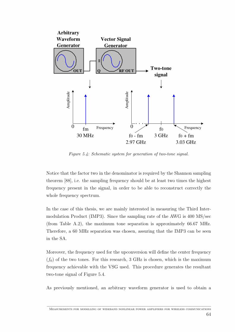
OUT
I
Q RF OUT
Arbitrary
Waveform
Generator
Vector Signal
Generator
Two-tone
signal
0 f m
30 MHz
0
f 0 - fm
2.97 GHz
f 0 + fm
3.03 GHz
f 0
3 GHz
A m
p l i
t u d
e
A m
p l i
t u d
e Frequency Frequency
Figure 5.4: Schematic system for generation of two-tone signal.
Notice that the factor two in the denominator is required by the Shannon sampling
theorem [88], i.e. the sampling frequency should be at least two times the highest
frequency present in the signal, in order to be able to reconstruct correctly the
whole frequency spectrum.
In the case of this thesis, we are mainly interested in measuring the Third Inter-
modulation Product (IMP3). Since the sampling rate of the AWG is 400 MS/sec
(from Table A.2), the maximum tone separation is approximately 66.67 MHz.
Therefore, a 60 MHz separation was chosen, assuring that the IMP3 can be seen
in the SA.
Moreover, the frequency used for the upconversion will define the center frequency
(f0) of the two tones. For this research, 3 GHz is chosen, which is the maximum
frequency achievable with the VSG used. This procedure generates the resultant
two-tone signal of Figure 5.4.
As previously mentioned, an arbitrary waveform generator is used to obtain a
Measurements for modelling of wideband nonlinear power amplifiers for wireless communications
64
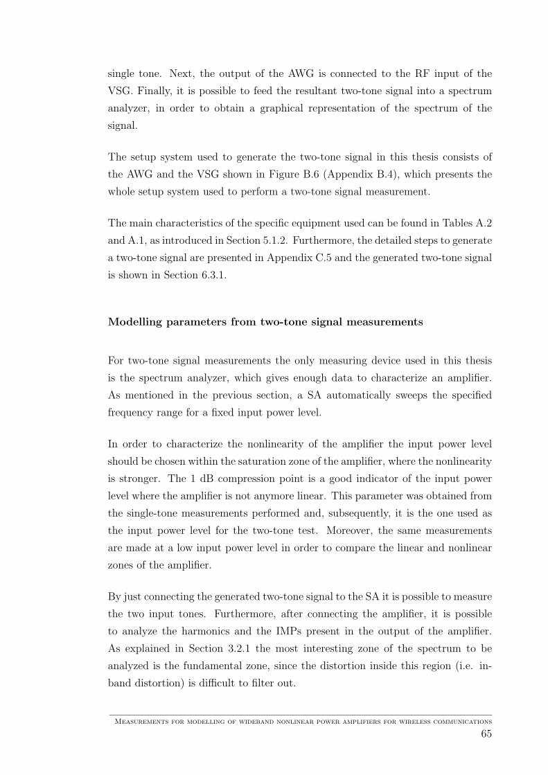
single tone. Next, the output of the AWG is connected to the RF input of the
VSG. Finally, it is possible to feed the resultant two-tone signal into a spectrum
analyzer, in order to obtain a graphical representation of the spectrum of the
signal.
The setup system used to generate the two-tone signal in this thesis consists of
the AWG and the VSG shown in Figure B.6 (Appendix B.4), which presents the
whole setup system used to perform a two-tone signal measurement.
The main characteristics of the specific equipment used can be found in Tables A.2
and A.1, as introduced in Section 5.1.2. Furthermore, the detailed steps to generate
a two-tone signal are presented in Appendix C.5 and the generated two-tone signal
is shown in Section 6.3.1.
Modelling parameters from two-tone signal measurements
For two-tone signal measurements the only measuring device used in this thesis
is the spectrum analyzer, which gives enough data to characterize an amplifier.
As mentioned in the previous section, a SA automatically sweeps the specified
frequency range for a fixed input power level.
In order to characterize the nonlinearity of the amplifier the input power level
should be chosen within the saturation zone of the amplifier, where the nonlinearity
is stronger. The 1 dB compression point is a good indicator of the input power
level where the amplifier is not anymore linear. This parameter was obtained from
the single-tone measurements performed and, subsequently, it is the one used as
the input power level for the two-tone test. Moreover, the same measurements
are made at a low input power level in order to compare the linear and nonlinear
zones of the amplifier.
By just connecting the generated two-tone signal to the SA it is possible to measure
the two input tones. Furthermore, after connecting the amplifier, it is possible
to analyze the harmonics and the IMPs present in the output of the amplifier.
As explained in Section 3.2.1 the most interesting zone of the spectrum to be
analyzed is the fundamental zone, since the distortion inside this region (i.e. in-
band distortion) is difficult to filter out.
Measurements for modelling of wideband nonlinear power amplifiers for wireless communications
65

Subsequently, the modelling parameters obtained and calculated from this two-
tone test are summarized in Table 5.2.
Table 5.2: Modelling parameters using two-tone input signals.
Type ofmeasurement
Modelling parameters
Frequency sweep ¦ Intermodulation products present in DC,(at low input fundamental, second and third harmonic zonespower level)Frequency sweep ¦ Plain two tones and spurious signals at DC(at 1 dB CP) fundamental, second and third harmonic zones
¦ Intermodulation products present in DC,fundamental, second and third harmonic zones
¦ Third Intermodulation Product (IMP3) in thefundamental zone
Calculated ¦ Intermodulation Distortion Ratio (PIMR)
Setup system and process to perform two-tone signal measurements
The setup system shown in Appendix B.4 consists of the setup system used to
generate a two-tone signal (i.e. AWG and VSG) and the testing system. The two-
tone signal is fed to the input of the amplifier, followed by the attenuators and
the measuring device. In this thesis, the measuring device is a spectrum analyzer,
which main specifications are summarized in Table A.4.
The process used in this research to measure the response of two-tone signals
passing through an amplifier is presented in Appendix C.6. Furthermore, the
modelling parameters obtained from the two-tone test are summarized in Sec-
tion 6.3.2.
Measurements for modelling of wideband nonlinear power amplifiers for wireless communications
66
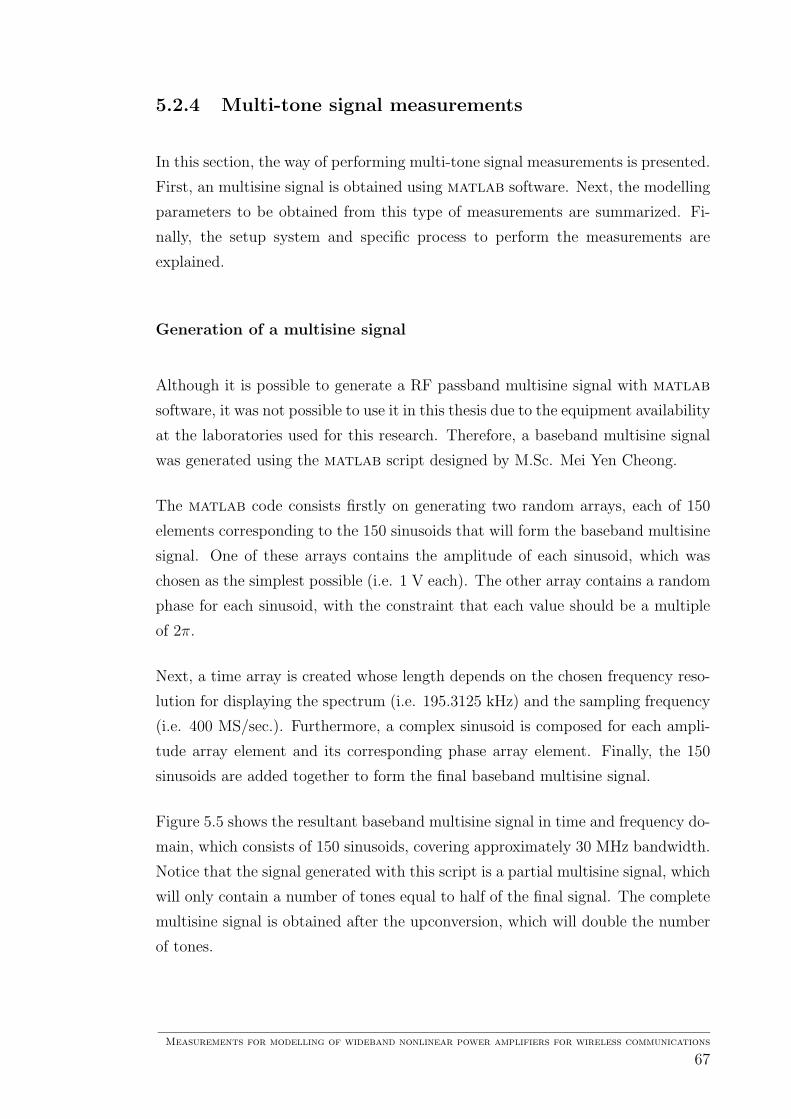
5.2.4 Multi-tone signal measurements
In this section, the way of performing multi-tone signal measurements is presented.
First, an multisine signal is obtained using matlab software. Next, the modelling
parameters to be obtained from this type of measurements are summarized. Fi-
nally, the setup system and specific process to perform the measurements are
explained.
Generation of a multisine signal
Although it is possible to generate a RF passband multisine signal with matlab
software, it was not possible to use it in this thesis due to the equipment availability
at the laboratories used for this research. Therefore, a baseband multisine signal
was generated using the matlab script designed by M.Sc. Mei Yen Cheong.
The matlab code consists firstly on generating two random arrays, each of 150
elements corresponding to the 150 sinusoids that will form the baseband multisine
signal. One of these arrays contains the amplitude of each sinusoid, which was
chosen as the simplest possible (i.e. 1 V each). The other array contains a random
phase for each sinusoid, with the constraint that each value should be a multiple
of 2π.
Next, a time array is created whose length depends on the chosen frequency reso-
lution for displaying the spectrum (i.e. 195.3125 kHz) and the sampling frequency
(i.e. 400 MS/sec.). Furthermore, a complex sinusoid is composed for each ampli-
tude array element and its corresponding phase array element. Finally, the 150
sinusoids are added together to form the final baseband multisine signal.
Figure 5.5 shows the resultant baseband multisine signal in time and frequency do-
main, which consists of 150 sinusoids, covering approximately 30 MHz bandwidth.
Notice that the signal generated with this script is a partial multisine signal, which
will only contain a number of tones equal to half of the final signal. The complete
multisine signal is obtained after the upconversion, which will double the number
of tones.
Measurements for modelling of wideband nonlinear power amplifiers for wireless communications
67

0 0.5 1 1.5 2 2.5−6
−4
−2
0
2
4
6
Time (ms)
Am
plitu
de (
V)
(a) Time domain
0 30 60 90 120 150−350
−300
−250
−200
−150
−100
−50
0
50
Frequency (MHz)
Out
put l
evel
(dB
m)
(b) Frequency domain
Figure 5.5: Baseband analog multisine signal obtained with matlab software.
Measurements for modelling of wideband nonlinear power amplifiers for wireless communications
68
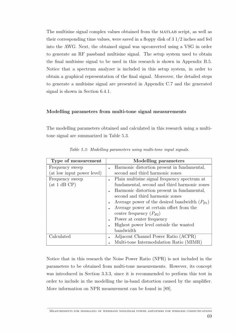
The multisine signal complex values obtained from the matlab script, as well as
their corresponding time values, were saved in a floppy disk of 3 1/2 inches and fed
into the AWG. Next, the obtained signal was upconverted using a VSG in order
to generate an RF passband multisine signal. The setup system used to obtain
the final multisine signal to be used in this research is shown in Appendix B.5.
Notice that a spectrum analyzer is included in this setup system, in order to
obtain a graphical representation of the final signal. Moreover, the detailed steps
to generate a multisine signal are presented in Appendix C.7 and the generated
signal is shown in Section 6.4.1.
Modelling parameters from multi-tone signal measurements
The modelling parameters obtained and calculated in this research using a multi-
tone signal are summarized in Table 5.3.
Table 5.3: Modelling parameters using multi-tone input signals.
Type of measurement Modelling parameters
Frequency sweep ¦ Harmonic distortion present in fundamental,(at low input power level) second and third harmonic zonesFrequency sweep ¦ Plain multisine signal frequency spectrum at(at 1 dB CP) fundamental, second and third harmonic zones
¦ Harmonic distortion present in fundamental,second and third harmonic zones
¦ Average power of the desired bandwidth (PB1)¦ Average power at certain offset from the
center frequency (PB2)¦ Power at center frequency¦ Highest power level outside the wanted
bandwidthCalculated ¦ Adjacent Channel Power Ratio (ACPR)
¦ Multi-tone Intermodulation Ratio (MIMR)
Notice that in this research the Noise Power Ratio (NPR) is not included in the
parameters to be obtained from multi-tone measurements. However, its concept
was introduced in Section 3.3.3, since it is recommended to perform this test in
order to include in the modelling the in-band distortion caused by the amplifier.
More information on NPR measurement can be found in [89].
Measurements for modelling of wideband nonlinear power amplifiers for wireless communications
69

Setup system and process to perform multi-tone signal measurements
Two-tone signals are a special case of multi-tone signals. Consequently, the setup
system to perform multi-tone measurements is the same than the one presented
in Appendix B.4 for two-tone signals. The only difference consists in the insertion
of the floppy disk containing the multisine signal generated with the matlab
script in to the diskette drive of the arbitrary waveform generator, as shown in
Appendix B.5.
Similarly, the process to perform any kind of multi-tone signal measurement is
the same followed for two-tone signal measurements, which is presented in Appen-
dix C.6. Finally, the measured and calculated multi-tone parameters can be found
in Section 6.4.2.
5.3 Summary of the chapter
This chapter described the necessary aspects to perform measurements of amplifier
nonlinearity. First, factors to take on count before measurements were introduced,
such as the needed characteristics of the input testing signal and a brief description
of the equipment to be used. The most important equipment specifications are
summarized in Appendix A. Furthermore, measuring devices calibration and noise
considerations were explained, which are planning matters important for the good
development of the measurements.
Finally, the procedure and setup systems to perform passive devices, single-, two-
and multi-tone signal measurements, as well as the way of generating two-tone and
multisine signals, were presented. Emphasis was made on the modelling parame-
ters to be obtained from single-, two- and multi-tone signal measurements, which
are summarized in Tables 5.1, 5.2 and 5.3, respectively.
Measurements for modelling of wideband nonlinear power amplifiers for wireless communications
70

Chapter 6
Power amplifier measurement
results
The measurements in this thesis have been performed as a practical approach
of the theory summarized in Chapters 2 to 5. Basic distortion measures of a
nonlinear amplifier using single-, two- and multi-tone input signals were obtained.
Mathematical analysis of these measures makes it possible to obtain more detailed
parameters, which can be used for modelling and linearization purposes.
In this chapter, the most important results obtained from each type of measure-
ment are presented. Due to its length, the complete set of data and plots can
be found in Appendix D. In some cases, it is not possible to obtain modelling
parameters directly from the measuring device. Therefore, the calculations and
parameters obtained from them are presented whenever necessary. Moreover, the
specific values used to setup the measuring devices in order to obtain the desired
parameters are presented. Finally, comments on the setup systems and the ob-
tained results are given.
Measurements for modelling of wideband nonlinear power amplifiers for wireless communications
71

6.1 Passive device measurements
In this thesis, extra devices have been divided into passive and auxiliary devices.
As introduced in Section 5.2.1, passive devices loss can be corrected in a high
degree by calibrating the measuring devices including all passive devices in the
process. On the other hand, attenuators are the only auxiliary devices used in
these measurements. Next, the results from the calibration of the network analyzer
and spectrum analyzer are presented, as well as the measured attenuation.
6.1.1 Devices needed to interconnect measuring systems
The processes presented in Appendix C.1 were followed in order to calibrate the
measuring devices. Next, the specific parameters and adapters used for calibrating
each device are presented. Moreover, the results after each calibration are shown
and explained.
Calibration of network analyzer
To perform measurements with the Network Analyzer (NWA) used in this thesis
(Table A.3), and according to the equipment availability, it was necessary to use
four adapters to connect the NWA’s end cable connectors to the attenuators and
amplifier. In addition to these, an extra adapter was necessary to perform the
calibration of the device. All the adapters used are shown in Figure 6.1. A more
detailed description of each type can be found in [90].
The process followed to calibrate the NWA is presented in Appendix C.1.1 and
the setup system used is shown in Appendix B.1.1. The values of the parameters
used for calibration are presented in Table 6.1.
It is important that the interpolation function is set to “ON” before calibration.
This function allows to make power-sweep measurements for different frequencies,
since it generates different sets of corrected data based on the set obtained from
the calibration process. In other words, the calibration system interpolates the
error terms whenever the stimulus parameters are changed.
Measurements for modelling of wideband nonlinear power amplifiers for wireless communications
72

APC 2.4 mm female
jack to APC 3.5 mm
male plug
SMA female jack to
SMA male plug
SMA female jack
to SMA female jack
(extra for calibration)
SMA male plug to
SMA female jack
APC 3.5 mm male
plug to APC 2.4 mm
female jack
Figure 6.1: Adapters used with a network analyzer for measurements and calibration ofthe device itself.
Table 6.1: Calibration parameters used for the network analyzer.
Parameter Value
Start frequency 1 GHzStop frequency 9 GHzPower level 0 dBmPower ONStart power -27 dBmStop power 3 dBmCenter frequency 5 GHzNumber of points 1401Calibration ONInterpolation ON
After the calibration was performed, the screen shown in Figure 6.2 was obtained
in the NWA when checking its calibration settings.
Figure 6.2: Network analyzer calibration settings.
Measurements for modelling of wideband nonlinear power amplifiers for wireless communications
73
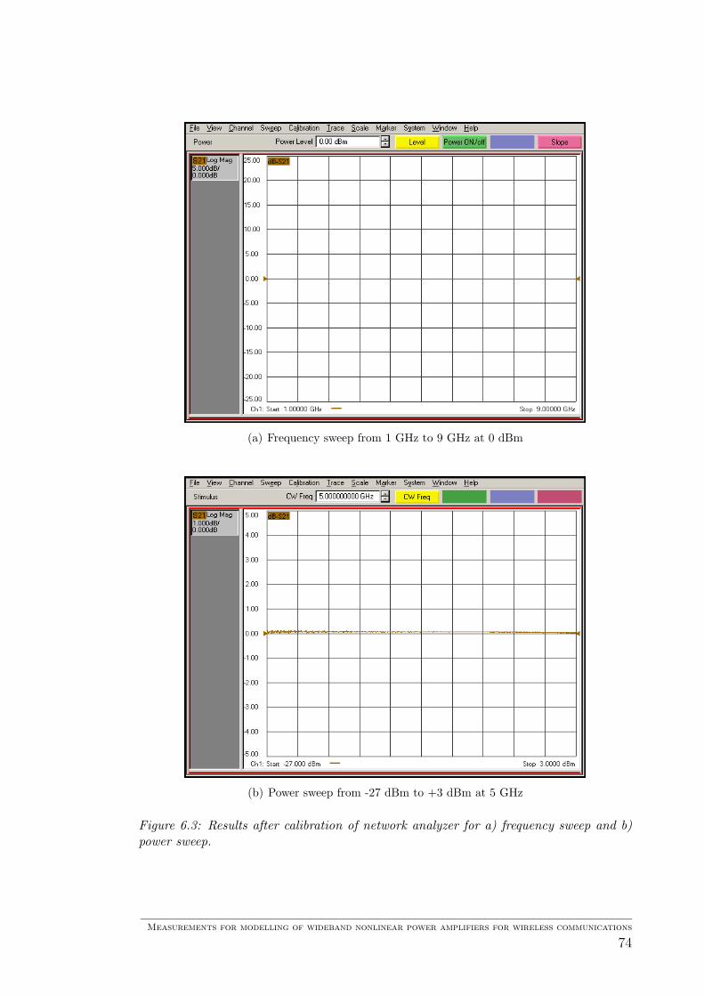
(a) Frequency sweep from 1 GHz to 9 GHz at 0 dBm
(b) Power sweep from -27 dBm to +3 dBm at 5 GHz
Figure 6.3: Results after calibration of network analyzer for a) frequency sweep and b)power sweep.
Measurements for modelling of wideband nonlinear power amplifiers for wireless communications
74

Next, frequency and power-sweep measurements were taken in order to check the
calibration results. As explained in Section 5.2.1, the ideal result after a calibration
is a flat trace of 0 dB gain for the frequency range calibrated. Figure 6.3(a) shows
that the maximum error after calibration is less than 0.05 dBm, which is very
small for the purposes of this thesis and when compared to the expected amplifier
gain of 30 dB.
In the same way, Figure 6.3(b) shows that, for a power sweep, the maximum
deviation from the ideal output expected after calibration is less than 0.15 dBm.
This error is considered small in this thesis since this maximum occurs at very low
input power levels, which might be confused with the inherent noise of the NWA.
However, when the input power level is increased the error becomes smaller, as
can be seen in Figure 6.3(b).
Calibration of spectrum analyzer
The calibration of the spectrum analyzer is only necessary when the ambient tem-
perature changes more than 10C [91], which is not the situation in the develop-
ment of this research since the laboratory where the equipment is placed has a
regulated temperature. However, the process to calibrate the SA can be found in
Appendix C.1.2 and can be performed as a way to test the correct functioning of
the device.
Since the SA does not have an error correction feature (like the one in the NWA), a
reference level measurement was performed in order to determine the attenuation
of the cables used for the measurements.
The setup system shown in Appendix B.1.2 was connected using the SA’s
−10 dBm/300 MHz calibration signal, the cables to be used and the same ex-
tra adapter used for the NWA’s calibration (Figure 6.1). The measurement of the
cables attenuation was performed following the process in Appendix C.2.
Figure 6.4 shows the results obtained. The signal amplitude measured is
−10.33 dBm. As previously mentioned, the amplitude of the input signal (i.e.
calibrating signal in SA) is −10 dBm. Consequently, the attenuation introduced
by the cables to the measuring system is 0.33 dBm. This attenuation has a small
Measurements for modelling of wideband nonlinear power amplifiers for wireless communications
75

effect on the measurements if compared with the 30 dB gain of the DUT. There-
fore, cable attenuation will not be included in further calculations. Nevertheless,
this attenuation should be considered when high accurate measurements are re-
quired.
Figure 6.4: Cable attenuation measurement performed with a spectrum analyzer.
6.1.2 Devices needed to perform correct measurements
The setup system shown in Appendix B.2 and the process presented in Appen-
dix C.3 were followed in order to measure the attenuators used in this research.
As an example of attenuation measurements, the result of a frequency sweep with
input power level of 0 dBm is presented in Figure 6.5(a). In the same way, a
power sweep with an input signal of 5 GHz gave the curve shown in Figure 6.5(b).
More examples of measurements of the attenuators with different input signals are
shown in Appendix D.1.
The attenuation obtained was in average -40.45 dB, which follows the expected
-40 dB. The maximum deviation was less than the specified total attenuation
accuracy range of ±1.3 dB (Table A.6). This means that the attenuators were
correctly measured and properly working for the rest of the measurements.
Measurements for modelling of wideband nonlinear power amplifiers for wireless communications
76
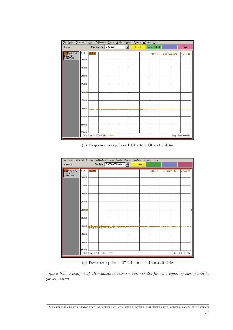
(a) Frequency sweep from 1 GHz to 9 GHz at 0 dBm
(b) Power sweep from -27 dBm to +3 dBm at 5 GHz
Figure 6.5: Example of attenuation measurement results for a) frequency sweep and b)power sweep.
Measurements for modelling of wideband nonlinear power amplifiers for wireless communications
77
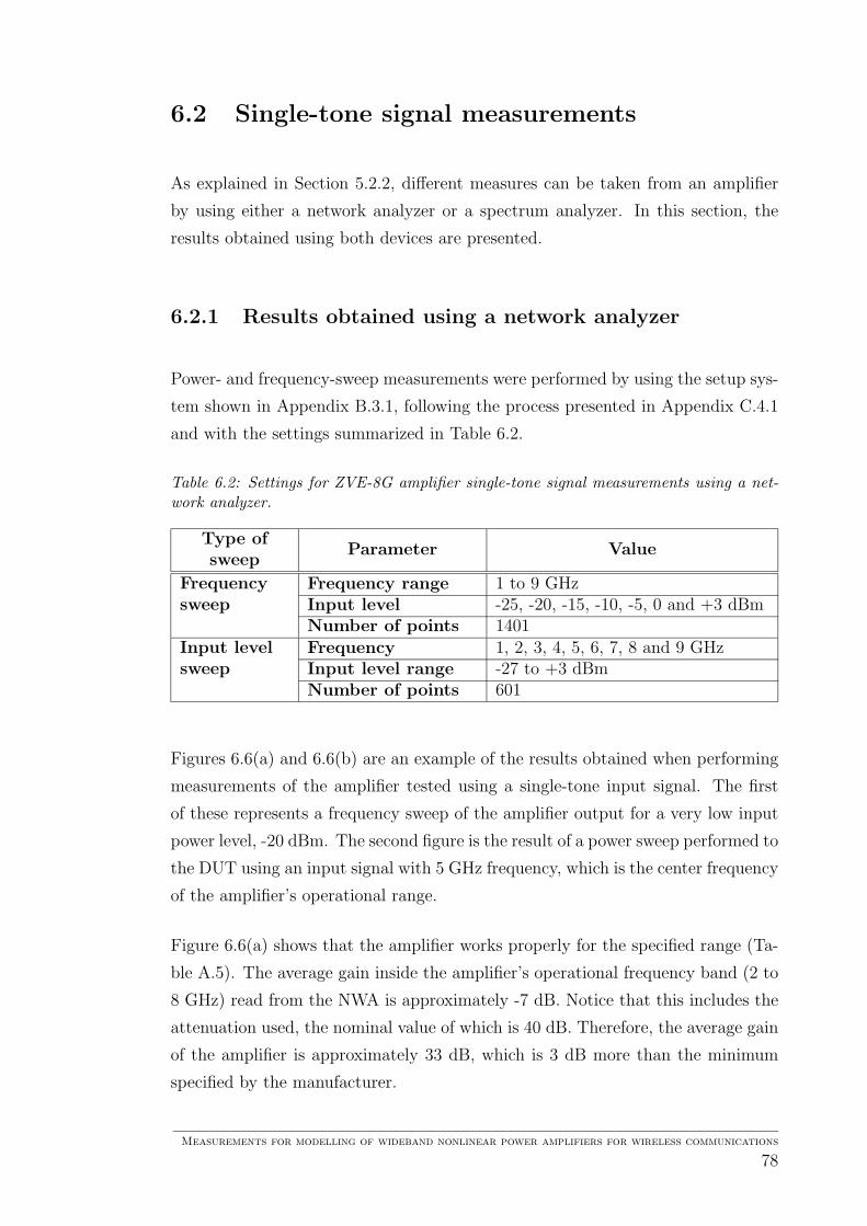
6.2 Single-tone signal measurements
As explained in Section 5.2.2, different measures can be taken from an amplifier
by using either a network analyzer or a spectrum analyzer. In this section, the
results obtained using both devices are presented.
6.2.1 Results obtained using a network analyzer
Power- and frequency-sweep measurements were performed by using the setup sys-
tem shown in Appendix B.3.1, following the process presented in Appendix C.4.1
and with the settings summarized in Table 6.2.
Table 6.2: Settings for ZVE-8G amplifier single-tone signal measurements using a net-work analyzer.
Type ofsweep
Parameter Value
Frequency Frequency range 1 to 9 GHzsweep Input level -25, -20, -15, -10, -5, 0 and +3 dBm
Number of points 1401Input level Frequency 1, 2, 3, 4, 5, 6, 7, 8 and 9 GHzsweep Input level range -27 to +3 dBm
Number of points 601
Figures 6.6(a) and 6.6(b) are an example of the results obtained when performing
measurements of the amplifier tested using a single-tone input signal. The first
of these represents a frequency sweep of the amplifier output for a very low input
power level, -20 dBm. The second figure is the result of a power sweep performed to
the DUT using an input signal with 5 GHz frequency, which is the center frequency
of the amplifier’s operational range.
Figure 6.6(a) shows that the amplifier works properly for the specified range (Ta-
ble A.5). The average gain inside the amplifier’s operational frequency band (2 to
8 GHz) read from the NWA is approximately -7 dB. Notice that this includes the
attenuation used, the nominal value of which is 40 dB. Therefore, the average gain
of the amplifier is approximately 33 dB, which is 3 dB more than the minimum
specified by the manufacturer.
Measurements for modelling of wideband nonlinear power amplifiers for wireless communications
78
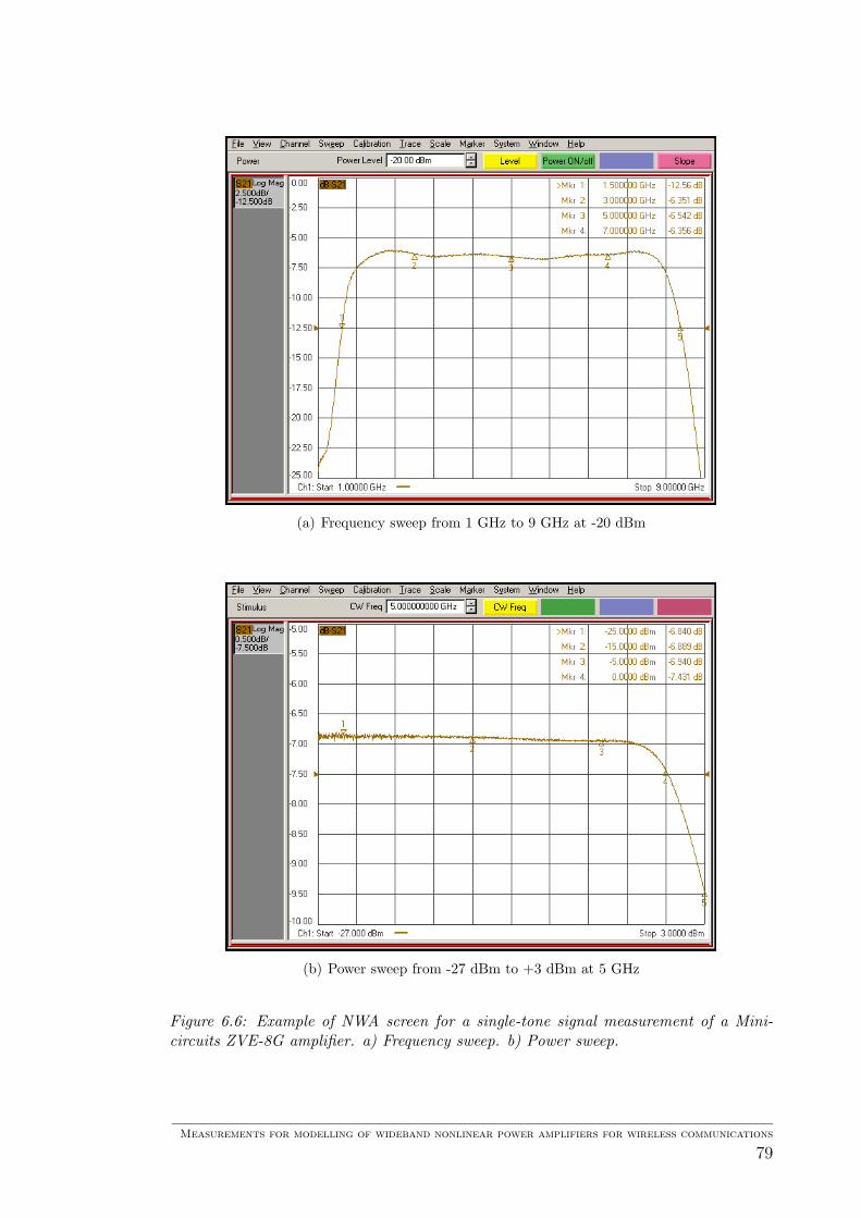
(a) Frequency sweep from 1 GHz to 9 GHz at -20 dBm
(b) Power sweep from -27 dBm to +3 dBm at 5 GHz
Figure 6.6: Example of NWA screen for a single-tone signal measurement of a Mini-circuits ZVE-8G amplifier. a) Frequency sweep. b) Power sweep.
Measurements for modelling of wideband nonlinear power amplifiers for wireless communications
79

On the other hand, the compression suffered by the amplifier at high input power
levels can be seen in Figure 6.6(b). Moreover, the linearity of the amplifier is
noticeable before the saturation zone. Screenshots of the NWA whilst performing
single-tone measurements with input signals outside the amplifier’s operational
range can be found in Appendix D.2.1.
A useful feature of the network analyzer used is that it can produce data files which
contain the measured points in a numeric format. As an example, Figure 6.7 shows
the file obtained when performing a frequency sweep with the NWA.
The most important information in these files are the first, fourth and fifth
columns. The first column register the measured stimulus, in this case the fre-
quency in hertz of the input signal applied to the amplifier. The fourth and fifth
columns represent, respectively, the real and imaginary components of the NWA’s
S21 corrected parameter, in this case the cascaded attenuators and amplifier out-
put.
Figure 6.7: Example of a data file obtained from the network analyzer. The first columnrefers to frequency in Hz and the third and fourth columns present, respectively, the realand imaginary parts of the corrected and measured S21 parameter.
The analysis of the measurements is easier with the data recorded from the NWA.
Figures 6.8(a) and Figure 6.8(b) show respectively the gain and phase curves ob-
tained from frequency-sweep measurements of different input power levels applied
to the tested amplifier. It is easily noticed that input power levels inside the li-
near zone behave in similar way and with approximately the same gain and phase.
However, as the input power level is increased, the amplifier approaches the satu-
Measurements for modelling of wideband nonlinear power amplifiers for wireless communications
80

ration zone and, therefore, the gain approaches zero. Moreover, the gain flatness
(i.e. variation of gain over the full operating frequency range) is approximately
0.96 dB, which falls inside the manufacturer specification (i.e. ±2 dB).
The process to generate these curves simply consists on calculating the gain and
the phase of each measured output point (S21 parameter in the NWA). In the case
of the gain, it is also necessary to add to each resultant the nominal attenuation
value (i.e. 40 dB) in order to obtained the real input-output relation for each
measured frequency. This whole process was easily done by using simple matlab
commands.
By manipulating the data obtained from the measurements performed with the
NWA it is possible to obtain the AM-AM and AM-PM characteristics of the tested
amplifier. The process is the same than the one used to produce the previous
frequency-sweep plots but using the power-sweep files.
Figure 6.9(a) shows a set of curves that represent the AM-AM characteristic of
the DUT for different input frequencies. The results show that for the frequencies
inside the operational range of the amplifier (i.e. 2 to 8 GHz) the curves behave
in similar manner. On the other hand, the curves outside this frequency range
have an unpredictable behavior and low gain (e.g. 1 GHz and 9 GHz curves in
Figure 6.9(a)). Moreover, it is easy to notice the linear and saturation zones of
the amplifier, which may slightly vary depending on the operating frequency.
The AM-PM characteristic of the amplifier tested for different input frequencies is
presented in Figure 6.9(b). Similarly to the AM-AM characteristic and according
to the expected results, the curves representing frequencies inside the amplifier’s
operational range behave linearly before the saturation zone, where it deviates
from the ideal flat line showing higher phase distortion. Moreover, it can be seen
that the frequencies outside the operational range have an undetermined behavior
with respect to their phase distortion.
The complete set of plots obtained from frequency and power-sweep measurements
can be found in Appendix D.2.2 and Appendix D.2.3, respectively.
Measurements for modelling of wideband nonlinear power amplifiers for wireless communications
81
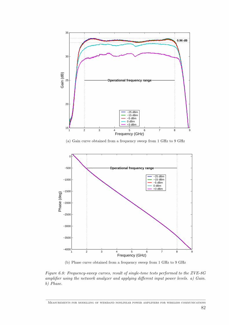
1 2 3 4 5 6 7 8 915
20
25
30
35
Frequency (GHz)
Gai
n (d
B)
0.96 dB
Operational frequency range
−25 dBm−15 dBm−5 dBm0 dBm+3 dBm
(a) Gain curve obtained from a frequency sweep from 1 GHz to 9 GHz
1 2 3 4 5 6 7 8 9−4000
−3500
−3000
−2500
−2000
−1500
−1000
−500
0
Frequency (GHz)
Pha
se (
deg)
Operational frequency range
−25 dBm−15 dBm−5 dBm0 dBm+3 dBm
(b) Phase curve obtained from a frequency sweep from 1 GHz to 9 GHz
Figure 6.8: Frequency-sweep curves, result of single-tone tests performed to the ZVE-8Gamplifier using the network analyzer and applying different input power levels. a) Gain.b) Phase.
Measurements for modelling of wideband nonlinear power amplifiers for wireless communications
82
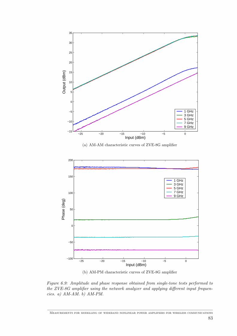
−25 −20 −15 −10 −5 0−15
−10
−5
0
5
10
15
20
25
30
35
Input (dBm)
Out
put (
dBm
)
1 GHz3 GHz5 GHz7 GHz9 GHz
(a) AM-AM characteristic curves of ZVE-8G amplifier
−25 −20 −15 −10 −5 0−100
−50
0
50
100
150
200
Input (dBm)
Pha
se (
deg)
1 GHz3 GHz5 GHz7 GHz9 GHz
(b) AM-PM characteristic curves of ZVE-8G amplifier
Figure 6.9: Amplitude and phase response obtained from single-tone tests performed tothe ZVE-8G amplifier using the network analyzer and applying different input frequen-cies. a) AM-AM. b) AM-PM.
Measurements for modelling of wideband nonlinear power amplifiers for wireless communications
83
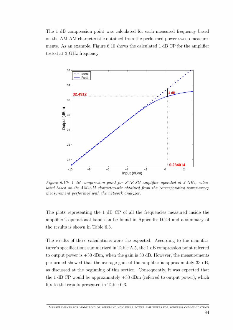
The 1 dB compression point was calculated for each measured frequency based
on the AM-AM characteristic obtained from the performed power-sweep measure-
ments. As an example, Figure 6.10 shows the calculated 1 dB CP for the amplifier
tested at 3 GHz frequency.
−10 −8 −6 −4 −2 0 2
24
26
28
30
32
34
36
Input (dBm)
Out
put (
dBm
)
1 dB
0.234014
32.4912
IdealReal
Figure 6.10: 1 dB compression point for ZVE-8G amplifier operated at 3 GHz, calcu-lated based on its AM-AM characteristic obtained from the corresponding power-sweepmeasurement performed with the network analyzer.
The plots representing the 1 dB CP of all the frequencies measured inside the
amplifier’s operational band can be found in Appendix D.2.4 and a summary of
the results is shown in Table 6.3.
The results of these calculations were the expected. According to the manufac-
turer’s specifications summarized in Table A.5, the 1 dB compression point referred
to output power is +30 dBm, when the gain is 30 dB. However, the measurements
performed showed that the average gain of the amplifier is approximately 33 dB,
as discussed at the beginning of this section. Consequently, it was expected that
the 1 dB CP would be approximately +33 dBm (referred to output power), which
fits to the results presented in Table 6.3.
Measurements for modelling of wideband nonlinear power amplifiers for wireless communications
84
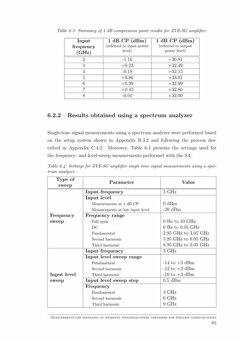
Table 6.3: Summary of 1 dB compression point results for ZVE-8G amplifier.
Inputfrequency
(GHz)
1 dB CP (dBm)(referred to input power
level)
1 dB CP (dBm)(referred to output
power level)
2 -1.16 +30.813 +0.23 +32.494 -0.19 +32.155 +0.86 +33.016 +0.99 +32.997 +0.43 +32.808 -0.01 +32.00
6.2.2 Results obtained using a spectrum analyzer
Single-tone signal measurements using a spectrum analyzer were performed based
on the setup system shown in Appendix B.3.2 and following the process des-
cribed in Appendix C.4.2. Moreover, Table 6.4 presents the settings used for
the frequency- and level-sweep measurements performed with the SA.
Table 6.4: Settings for ZVE-8G amplifier single-tone signal measurements using a spec-trum analyzer.
Type ofsweep
Parameter Value
Input frequency 3 GHzInput level
Measurements at 1 dB CP 0 dBmMeasurements at low input level -20 dBm
Frequency Frequency rangesweep Full span 0 Hz to 10 GHz
DC 0 Hz to 0.05 GHzFundamental 2.95 GHz to 3.05 GHzSecond harmonic 5.95 GHz to 6.05 GHzThird harmonic 8.95 GHz to 9.05 GHz
Input frequency 3 GHzInput level sweep range
Fundamental -14 to +3 dBmSecond harmonic -12 to +3 dBm
Input level Third harmonic -10 to +3 dBmsweep Input level sweep step 0.5 dBm
FrequencyFundamental 3 GHzSecond harmonic 6 GHzThird harmonic 9 GHz
Measurements for modelling of wideband nonlinear power amplifiers for wireless communications
85
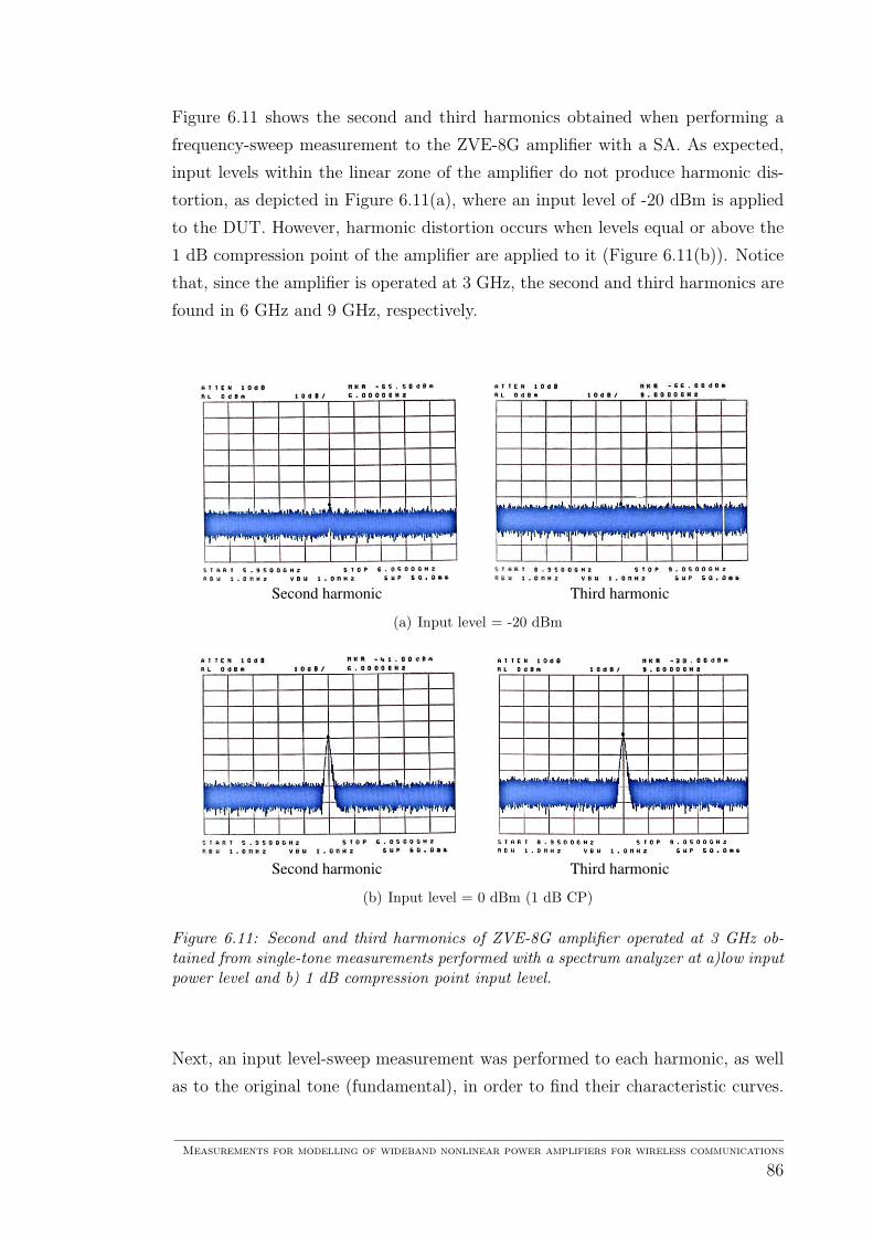
Figure 6.11 shows the second and third harmonics obtained when performing a
frequency-sweep measurement to the ZVE-8G amplifier with a SA. As expected,
input levels within the linear zone of the amplifier do not produce harmonic dis-
tortion, as depicted in Figure 6.11(a), where an input level of -20 dBm is applied
to the DUT. However, harmonic distortion occurs when levels equal or above the
1 dB compression point of the amplifier are applied to it (Figure 6.11(b)). Notice
that, since the amplifier is operated at 3 GHz, the second and third harmonics are
found in 6 GHz and 9 GHz, respectively.
Second harmonic Third harmonic
(a) Input level = -20 dBm
Second harmonic Third harmonic
(b) Input level = 0 dBm (1 dB CP)
Figure 6.11: Second and third harmonics of ZVE-8G amplifier operated at 3 GHz ob-tained from single-tone measurements performed with a spectrum analyzer at a)low inputpower level and b) 1 dB compression point input level.
Next, an input level-sweep measurement was performed to each harmonic, as well
as to the original tone (fundamental), in order to find their characteristic curves.
Measurements for modelling of wideband nonlinear power amplifiers for wireless communications
86
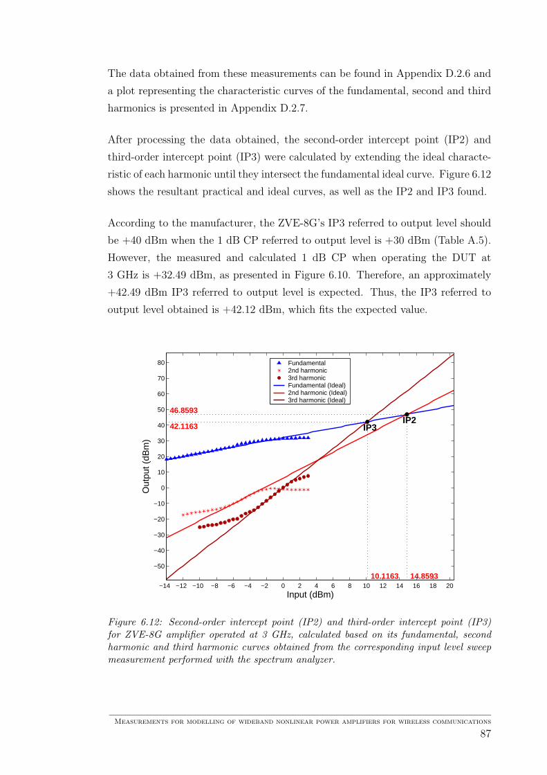
The data obtained from these measurements can be found in Appendix D.2.6 and
a plot representing the characteristic curves of the fundamental, second and third
harmonics is presented in Appendix D.2.7.
After processing the data obtained, the second-order intercept point (IP2) and
third-order intercept point (IP3) were calculated by extending the ideal characte-
ristic of each harmonic until they intersect the fundamental ideal curve. Figure 6.12
shows the resultant practical and ideal curves, as well as the IP2 and IP3 found.
According to the manufacturer, the ZVE-8G’s IP3 referred to output level should
be +40 dBm when the 1 dB CP referred to output level is +30 dBm (Table A.5).
However, the measured and calculated 1 dB CP when operating the DUT at
3 GHz is +32.49 dBm, as presented in Figure 6.10. Therefore, an approximately
+42.49 dBm IP3 referred to output level is expected. Thus, the IP3 referred to
output level obtained is +42.12 dBm, which fits the expected value.
−14 −12 −10 −8 −6 −4 −2 0 2 4 6 8 10 12 14 16 18 20
−50
−40
−30
−20
−10
0
10
20
30
40
50
60
70
80
Input (dBm)
Out
put (
dBm
)
14.859310.1163
46.8593
42.1163IP2
IP3
Fundamental2nd harmonic3rd harmonicFundamental (Ideal)2nd harmonic (Ideal)3rd harmonic (Ideal)
Figure 6.12: Second-order intercept point (IP2) and third-order intercept point (IP3)for ZVE-8G amplifier operated at 3 GHz, calculated based on its fundamental, secondharmonic and third harmonic curves obtained from the corresponding input level sweepmeasurement performed with the spectrum analyzer.
Measurements for modelling of wideband nonlinear power amplifiers for wireless communications
87
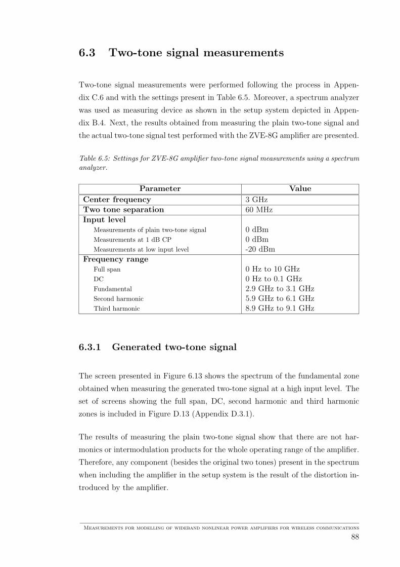
6.3 Two-tone signal measurements
Two-tone signal measurements were performed following the process in Appen-
dix C.6 and with the settings present in Table 6.5. Moreover, a spectrum analyzer
was used as measuring device as shown in the setup system depicted in Appen-
dix B.4. Next, the results obtained from measuring the plain two-tone signal and
the actual two-tone signal test performed with the ZVE-8G amplifier are presented.
Table 6.5: Settings for ZVE-8G amplifier two-tone signal measurements using a spectrumanalyzer.
Parameter Value
Center frequency 3 GHzTwo tone separation 60 MHzInput level
Measurements of plain two-tone signal 0 dBmMeasurements at 1 dB CP 0 dBmMeasurements at low input level -20 dBm
Frequency rangeFull span 0 Hz to 10 GHzDC 0 Hz to 0.1 GHzFundamental 2.9 GHz to 3.1 GHzSecond harmonic 5.9 GHz to 6.1 GHzThird harmonic 8.9 GHz to 9.1 GHz
6.3.1 Generated two-tone signal
The screen presented in Figure 6.13 shows the spectrum of the fundamental zone
obtained when measuring the generated two-tone signal at a high input level. The
set of screens showing the full span, DC, second harmonic and third harmonic
zones is included in Figure D.13 (Appendix D.3.1).
The results of measuring the plain two-tone signal show that there are not har-
monics or intermodulation products for the whole operating range of the amplifier.
Therefore, any component (besides the original two tones) present in the spectrum
when including the amplifier in the setup system is the result of the distortion in-
troduced by the amplifier.
Measurements for modelling of wideband nonlinear power amplifiers for wireless communications
88

Figure 6.13: Frequency spectrum of the fundamental zone of the generated two-tonesignal obtained with a spectrum analyzer. The two-tone signal has a center frequency of3 GHz, tone separation of 60 MHz and it is tested at a high input power level equal tothe 1 dB CP of the DUT (0 dBm).
6.3.2 Two-tone signal applied to amplifier
The two-tone signal of Figure 6.13 was applied as input signal to the ZVE-8G
amplifier. When the level of the input signal is low, no harmonic or intermodulation
distortion affects the operation of the amplifier, as presented in Figure 6.14, which
shows the frequency spectrum of the measured full span of the DUT operated at
3 GHz and -20 dBm input level.
Figure 6.14: Frequency spectrum of the measured full span of ZVE-8G amplifier obtainedfrom a two-tone signal measurement. The input signal has a low input power level equalto -20 dBm.
Measurements for modelling of wideband nonlinear power amplifiers for wireless communications
89

On the other hand, Figure 6.15 shows the distortion caused by the amplifier for
high input levels (≥1 dB CP). The data obtained from two-tone signal measure-
ments, as well as the full set of screens, can be found in Appendix D.3.
DC Fundamental
Second harmonic Third harmonic
Figure 6.15: Intermodulation products present at DC, fundamental, second harmonic andthird harmonic zones of ZVE-8G amplifier obtained from two-tone signal measurementsperformed with a spectrum analyzer. The two-tone input signal has a center frequencyof 3 GHz, tone separation of 60 MHz and input power level equal to the DUT’s 1 dBcompression point input level (0 dBm).
Table 6.6 summarizes the frequency components measured in the fundamental,
second and third harmonic zones of the ZVE-8G amplifier when operating it at a
high input level equal to its 1 dB CP. A plot of the reconstruction of the spectrum
based on this data is included in Appendix D.3.3.
An important parameter obtained from Table 6.6 is the third intermodulation
product (IMP3) in the fundamental zone. The IMP3 is the frequency component
closest to the original tones and, therefore, it is difficult to filter out.
Measurements for modelling of wideband nonlinear power amplifiers for wireless communications
90
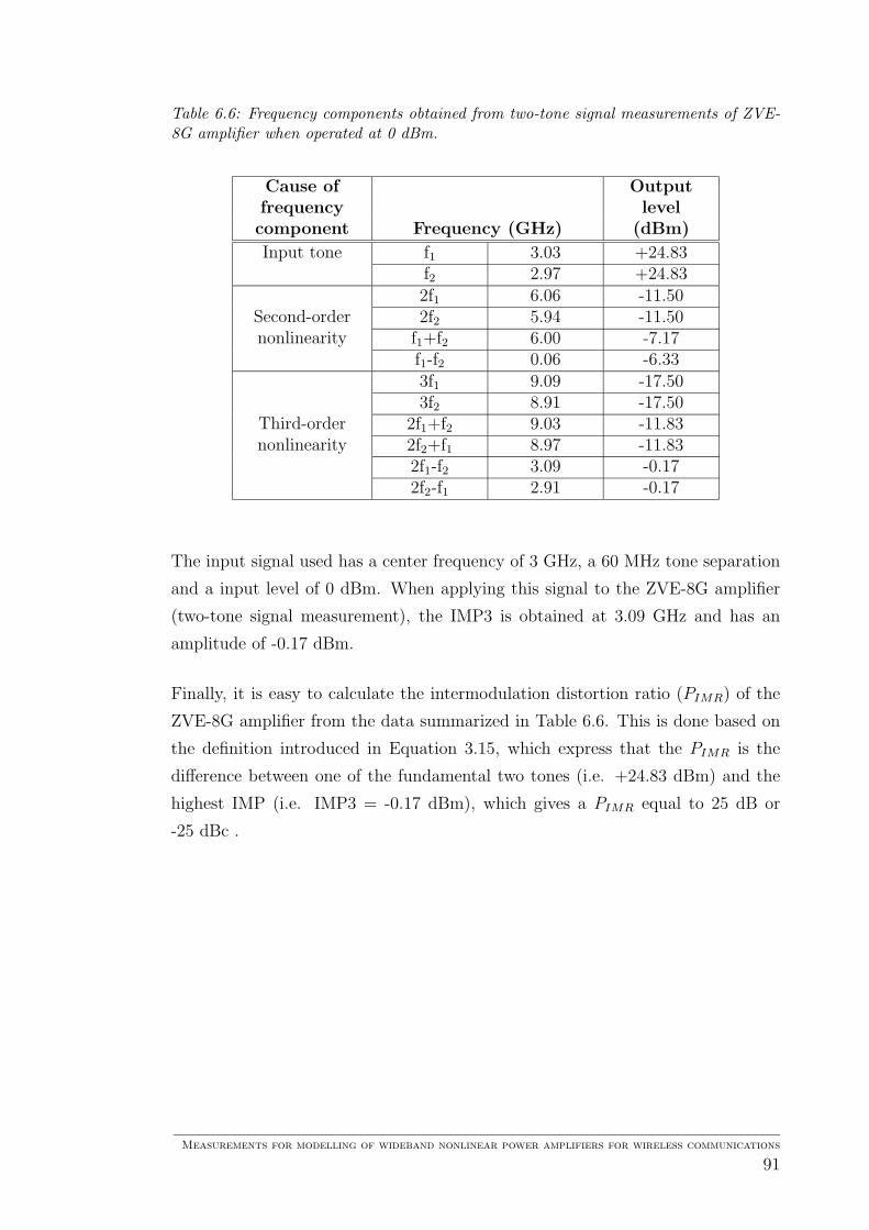
Table 6.6: Frequency components obtained from two-tone signal measurements of ZVE-8G amplifier when operated at 0 dBm.
Cause offrequency
Outputlevel
component Frequency (GHz) (dBm)
Input tone f1 3.03 +24.83f2 2.97 +24.832f1 6.06 -11.50
Second-order 2f2 5.94 -11.50nonlinearity f1+f2 6.00 -7.17
f1-f2 0.06 -6.333f1 9.09 -17.503f2 8.91 -17.50
Third-order 2f1+f2 9.03 -11.83nonlinearity 2f2+f1 8.97 -11.83
2f1-f2 3.09 -0.172f2-f1 2.91 -0.17
The input signal used has a center frequency of 3 GHz, a 60 MHz tone separation
and a input level of 0 dBm. When applying this signal to the ZVE-8G amplifier
(two-tone signal measurement), the IMP3 is obtained at 3.09 GHz and has an
amplitude of -0.17 dBm.
Finally, it is easy to calculate the intermodulation distortion ratio (PIMR) of the
ZVE-8G amplifier from the data summarized in Table 6.6. This is done based on
the definition introduced in Equation 3.15, which express that the PIMR is the
difference between one of the fundamental two tones (i.e. +24.83 dBm) and the
highest IMP (i.e. IMP3 = -0.17 dBm), which gives a PIMR equal to 25 dB or
-25 dBc .
Measurements for modelling of wideband nonlinear power amplifiers for wireless communications
91
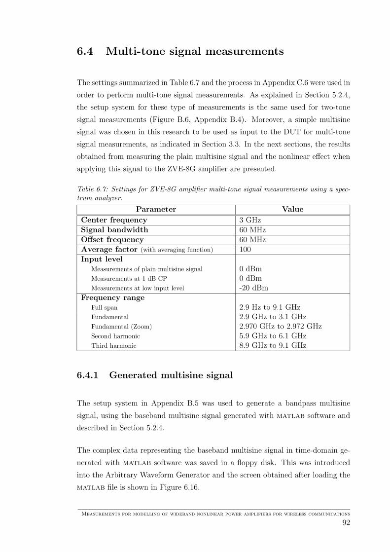
6.4 Multi-tone signal measurements
The settings summarized in Table 6.7 and the process in Appendix C.6 were used in
order to perform multi-tone signal measurements. As explained in Section 5.2.4,
the setup system for these type of measurements is the same used for two-tone
signal measurements (Figure B.6, Appendix B.4). Moreover, a simple multisine
signal was chosen in this research to be used as input to the DUT for multi-tone
signal measurements, as indicated in Section 3.3. In the next sections, the results
obtained from measuring the plain multisine signal and the nonlinear effect when
applying this signal to the ZVE-8G amplifier are presented.
Table 6.7: Settings for ZVE-8G amplifier multi-tone signal measurements using a spec-trum analyzer.
Parameter Value
Center frequency 3 GHzSignal bandwidth 60 MHzOffset frequency 60 MHzAverage factor (with averaging function) 100Input level
Measurements of plain multisine signal 0 dBmMeasurements at 1 dB CP 0 dBmMeasurements at low input level -20 dBm
Frequency rangeFull span 2.9 Hz to 9.1 GHzFundamental 2.9 GHz to 3.1 GHzFundamental (Zoom) 2.970 GHz to 2.972 GHzSecond harmonic 5.9 GHz to 6.1 GHzThird harmonic 8.9 GHz to 9.1 GHz
6.4.1 Generated multisine signal
The setup system in Appendix B.5 was used to generate a bandpass multisine
signal, using the baseband multisine signal generated with matlab software and
described in Section 5.2.4.
The complex data representing the baseband multisine signal in time-domain ge-
nerated with matlab software was saved in a floppy disk. This was introduced
into the Arbitrary Waveform Generator and the screen obtained after loading the
matlab file is shown in Figure 6.16.
Measurements for modelling of wideband nonlinear power amplifiers for wireless communications
92
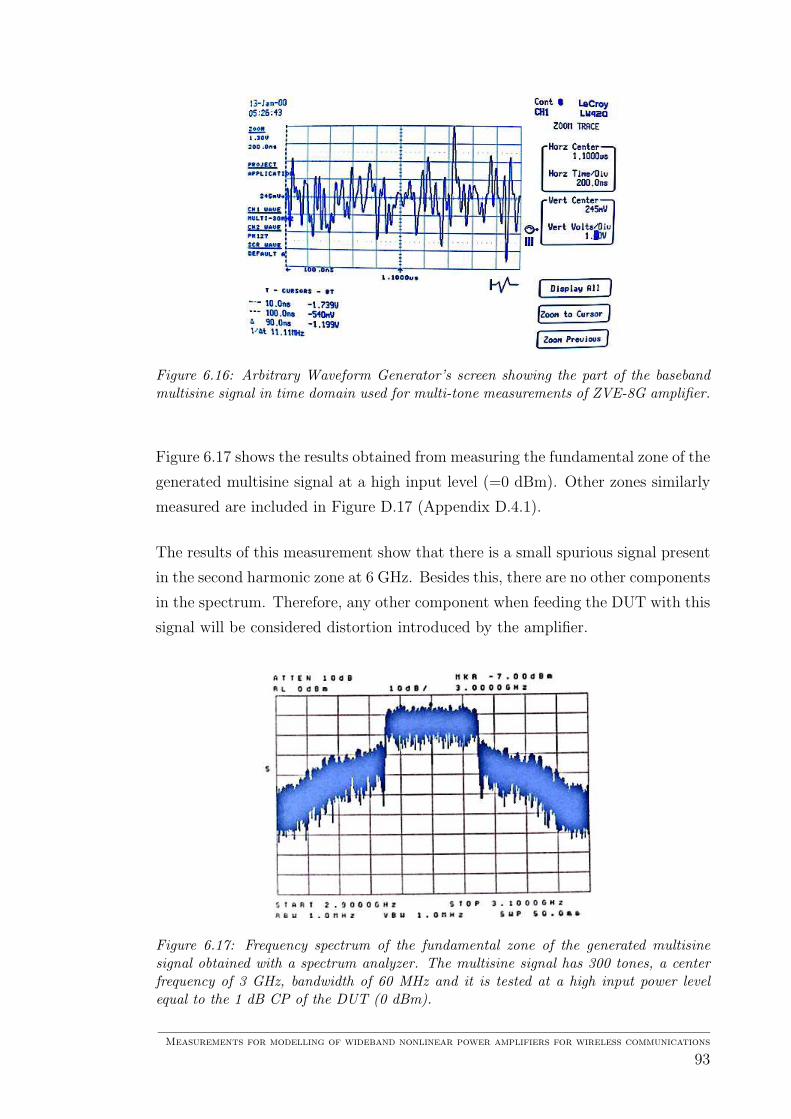
Figure 6.16: Arbitrary Waveform Generator’s screen showing the part of the basebandmultisine signal in time domain used for multi-tone measurements of ZVE-8G amplifier.
Figure 6.17 shows the results obtained from measuring the fundamental zone of the
generated multisine signal at a high input level (=0 dBm). Other zones similarly
measured are included in Figure D.17 (Appendix D.4.1).
The results of this measurement show that there is a small spurious signal present
in the second harmonic zone at 6 GHz. Besides this, there are no other components
in the spectrum. Therefore, any other component when feeding the DUT with this
signal will be considered distortion introduced by the amplifier.
Figure 6.17: Frequency spectrum of the fundamental zone of the generated multisinesignal obtained with a spectrum analyzer. The multisine signal has 300 tones, a centerfrequency of 3 GHz, bandwidth of 60 MHz and it is tested at a high input power levelequal to the 1 dB CP of the DUT (0 dBm).
Measurements for modelling of wideband nonlinear power amplifiers for wireless communications
93

6.4.2 Multisine signal applied to amplifier
Multi-tone measurements were performed by applying the multisine signal of Fi-
gure 6.17 as input signal to the ZVE-8G amplifier. Next, the results of these mea-
surements are presented using examples whenever possible. The data obtained
from multi-tone signal measurements, as well as the full set of screens, can be
found in Appendix D.4.
As an example of the results obtained for low input power levels, Figure 6.18 shows
the frequency spectrum for the measured full span of the DUT operated -20 dBm
input level. This input level falls into the linear zone of the amplifier. Therefore,
no harmonic distortion affects the operation of the amplifier, which means that
there are not frequency components, others than the original and the spurious at
6 GHz, in the resultant frequency spectrum.
Figure 6.18: Frequency spectrum of the measured full span of ZVE-8G amplifier obtainedfrom a multi-tone signal measurement. The input signal has a low input power level equalto -20 dBm.
As previously explained, for low input levels there is not distortion components
introduced by the amplifier. However, when the DUT is operated at high input
levels (≥1 dB CP), harmonic distortion is present in the resultant spectrum, as
shown in the example of Figure 6.19.
Measurements for modelling of wideband nonlinear power amplifiers for wireless communications
94

Second harmonic Third harmonic
Fundamental
Figure 6.19: Frequency spectrum of the fundamental, second harmonic and third har-monic zones of ZVE-8G amplifier obtained from multi-tone signal measurements per-formed with a spectrum analyzer. The multisine input signal has a center frequency of3 GHz, bandwidth of 60 MHz and input power level equal to the DUT’s 1 dB compressionpoint input level (0 dBm).
In order to calculate the Adjacent Channel Power Ratio (ACPR) of an amplifier it
is necessary to measure the average power of the desired bandwidth (PB1) and the
average power at certain offset from the center frequency (PB2) when performing
a multi-tone signal measurement. Figure 6.20 presents an example of these mea-
surements. The average power was obtained by using the SA’s averaging function
with an average factor of 100. PB1 was measured at the center frequency of the
input multisine signal, 3 GHz.
On the other hand, the offset to be used for measuring PB2 should be equal to
the channel spacing specified for a transmission scheme. Generally, when the pur-
pose of the measurements is to model the behavior of an amplifier, a transmission
scheme is not specified and, consequently, there is not a specific channel spacing.
Therefore, and in order to model the worst case scenario, the channel spacing
should be chosen as equal to the bandwidth of the multi-tone signal. Thus, the
offset was chosen as 60 MHz and, subsequently, the average power PB2 was mea-
sured at 2.94 GHz.
Measurements for modelling of wideband nonlinear power amplifiers for wireless communications
95
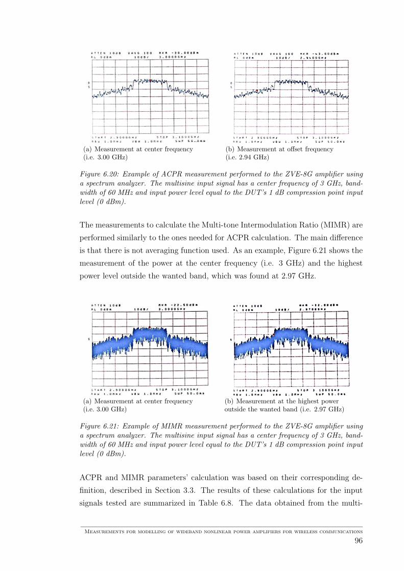
(a) Measurement at center frequency(i.e. 3.00 GHz)
(b) Measurement at offset frequency(i.e. 2.94 GHz)
Figure 6.20: Example of ACPR measurement performed to the ZVE-8G amplifier usinga spectrum analyzer. The multisine input signal has a center frequency of 3 GHz, band-width of 60 MHz and input power level equal to the DUT’s 1 dB compression point inputlevel (0 dBm).
The measurements to calculate the Multi-tone Intermodulation Ratio (MIMR) are
performed similarly to the ones needed for ACPR calculation. The main difference
is that there is not averaging function used. As an example, Figure 6.21 shows the
measurement of the power at the center frequency (i.e. 3 GHz) and the highest
power level outside the wanted band, which was found at 2.97 GHz.
(a) Measurement at center frequency(i.e. 3.00 GHz)
(b) Measurement at the highest poweroutside the wanted band (i.e. 2.97 GHz)
Figure 6.21: Example of MIMR measurement performed to the ZVE-8G amplifier usinga spectrum analyzer. The multisine input signal has a center frequency of 3 GHz, band-width of 60 MHz and input power level equal to the DUT’s 1 dB compression point inputlevel (0 dBm).
ACPR and MIMR parameters’ calculation was based on their corresponding de-
finition, described in Section 3.3. The results of these calculations for the input
signals tested are summarized in Table 6.8. The data obtained from the multi-
Measurements for modelling of wideband nonlinear power amplifiers for wireless communications
96

tone measurements performed, used to calculate ACPR and MIMR can be found
in Appendix D.4.2.
The results presented in Table 6.8, show the expected behavior. ACPR and MIMR
get higher (referenced to the carrier power) as the nonlinearity of the amplifier is
increased (i.e. input level is increased inside the saturation zone), which means
that the distortion outside the desired band gets stronger.
Table 6.8: Results of Adjacent Channel Power Ratio (ACPR) and Multi-tone Intermo-dulation Ratio (MIMR) calculations. The data was obtained using a spectrum analyzerand a multisine input signal.
Signal measured ACPR (dBc) MIMR (dBc)
Plain multisine input signal(at 1 dB CP = 0 dBm) -28.33 -17.33
Input signal applied to DUT(at low input level = -20 dBm) -25.50 -16.00
Input signal applied to DUT(at 1 dB CP = 0 dBm) -13.00 -9.50
6.5 Summary of the chapter
This chapter presents the results of practical measurements based on the theory
and procedures described in Chapters 2 to 5. The setup systems and processes
used for all the measurements are compiled in Appendix B and C, respectively.
Moreover, the figures, data and plots (others than the presented in this chapter)
obtained from the tests can be found in Appendix D.
The results of passive devices were good. After the calibration of the Network
Analyzer (NWA) the maximum deviation from the ideal flat frequency-sweep trace
was 0.05 dB, which is considered small when compared to the amplifier’s specified
gain (i.e. 30 dB). The calibration of the Spectrum Analyzer (SA) was performed
in order to check the correct functioning of the device. Cable attenuation was
measured with the spectrum analyzer, giving a 0.33 dB result. Furthermore, the
measured attenuators nominal value was 40.45 dB, which is correct according to
the specified by the manufacturer (i.e. 40±1.3 dB).
Measurements for modelling of wideband nonlinear power amplifiers for wireless communications
97
Different parameters were obtained using single-tone input signals with a NWA and
a SA. The results were good and inside the amplifier manufacturer’s specifications.
The average gain obtained inside the amplifier’s operational range (i.e. 2 to 8 GHz)
was 33 dB (3 dB more than the minimum specified). From the NWA, frequency-
sweep, AM-AM and AM-PM curves were depicted and the 1 dB compression point
(1 dB CP) was calculated for each of the frequencies measured (results summarized
in Table 6.3). As an example of the reliability of the results obtained from these
measurements, the output 1 dB compression point for a 3 GHz input signal was
+32.49 dBm. The value of this parameter found in the specifications is +30 dB
when the gain of the amplifier is 30 dB. Therefore, the 1 dB CP obtained is
approximately the expected, based on the measured gain (i.e. 33 dB).
With the SA and an input signal of 3 GHz and 0 dBm, the second- and third-
harmonic curves of the ZVE-8G amplifier were obtained and the corresponding
second-order intercept point (IP2) and third-order intercept point(IP3) were cal-
culated. From these, the obtained output IP3 (i.e. +42.12 dBm) was compared
with the expected value (+42.49 dBm), giving a positive result.
The generated signal to be used as input for the two-tone signal measurement was
measured, giving as result components in the two expected frequencies. No other
components were detected for low or high input levels. Therefore, when using
this signal as input to the amplifier tested, any component shown in the output
spectrum will be distortion introduced by the amplifier. Next, the two-tone signal
measurement was performed. The harmonics and intermodulation products were
summarized in Table 6.6 and the intermodulation distortion ratio was calculated,
giving a result of 25 dB.
In order to perform multi-tone signal measurements, a multisine signal was used,
which was measured as well, giving as result the expected spectrum in the fun-
damental zone and a spurious signal in the second harmonic zone. The resultant
spectrum when applying the multisine signal to the amplifier showed no harmonic
distortion for low input power levels and strong distortion for high input levels
(≥1 dB CP), as theoretically predicted. Finally, calculations of the adjacent power
channel ratio and the multi-tone intermodulation ratio showed the expected be-
havior, giving higher levels (referenced to the carrier power) for high input levels,
consequently causing higher nonlinear distortion.
Measurements for modelling of wideband nonlinear power amplifiers for wireless communications
98
Chapter 7
Measurement errors and use of
results
The theory summarized in this thesis was taken to practice in Chapter 6, where
measurements of amplifier nonlinearity were performed. Single-, two- and multi-
tone signals were used in order to obtain different measures and parameters that
are useful for modelling and, furthermore, alleviating the distortion caused by
amplifiers.
In this chapter, two main factors to consider after the performed measurements in
this research are covered. First, an analysis of the possible errors that may have
occurred during the planning and measurement process is done. This analysis
is based on experiences and knowledge acquired during the whole measurement
process. The second aspect to be considered in this chapter is the usefulness of
the measurements, which is supported by an actual example of the application of
the results in modelling the measured amplifier. Finally, examples of the general
use of amplifier measurements are commented and references for these are given.
Measurements for modelling of wideband nonlinear power amplifiers for wireless communications
99

7.1 Discussion of measurement errors
Making accurate measurements is a difficult task since it requires precision during
the whole process of planning, selecting the adequate devices, connecting systems
and reading results. Therefore, the error analysis is a complex process, which
involves a big amount of factors, from connection mismatches to implicit errors in
the measuring devices. This is why, in this section, the intention is not to quantify
the error obtained while performing the measurements but to analyze the possible
causes of these errors and to give recommendations for future measurements which
might require a higher accuracy.
On the statistical point of view, it has been calculated that higher-order Intermo-
dulation Products (IMPs) have higher variance. Therefore, low-order IMPs can
be measured accurately while higher-order ones give more problems. Fortunately,
the lower-order IMPs (usually IMP3) are the main focus of the measurements, as
pointed out in Section 3.2.1. Moreover, it is possible to adjust the variance of the
IMP3 by proper biasing of the amplifier and to fine-tune the phase-shift in order
to obtain more accurate measurement results [92].
Next, the most common error factors occurring during the practical measure-
ments are commented. The first obvious aspect influencing the accuracy of the
measurements is the accuracy of the measuring devices (i.e. network analyzer and
spectrum analyzer). For low input levels the accuracy of the results is limited
by the device’s floor noise and magnitude and phase uncertainty. For high input
levels, compression limits the accuracy. Moreover, generators (i.e. arbitrary wave-
form generator and vector signal generator) can affect the results by introducing
subharmonics and spurious signals.
Before calibrating or measuring, check that all cables and adapters are correctly
tightened in order to avoid errors due to mismatches. If the effect of mismatches
cannot be neglected, it should be kept as constant as possible. This should be
taken into account during the calibration and the measurement itself.
Using an extra adapter when calibrating the measuring devices can produce errors
in measurements. However, in my personal experience, loss due to connectors
when calibrating is higher if an adapter is taken out of the calibration system
Measurements for modelling of wideband nonlinear power amplifiers for wireless communications
100
instead of adding one. In general, the loss caused by adapters is usually very low
(≈< 0.15 dBm). This loss can be minimized by using as few parts as possible.
Moreover, calibration should be done without attenuators, in order to avoid errors
caused by very low power signals confused with the measuring device’s intrinsic
noise.
In the specific case of amplifier measurements, it is highly recommended to make
sure that the amplifier is connected to the system before feeding it with the power
supply. Likewise, it is important not to forget to turn off the power supply of
the amplifier, when finishing working with it. This simple precautions will avoid
damaging the device and, subsequently, erroneous results.
Attention should be paid when setting the measuring devices to obtain a specific
parameter. First, calibration of the measuring device should be correctly done. In
the case of measurements with a network analyzer, the interpolation and correction
features should be turned on before performing any power- or frequency-sweep. On
the other hand, when working with the spectrum analyzer, the “RF output” of the
vector signal generator should be active and for two- and multi-tone measurements
the “Vector” function should be turned on as well.
Other errors in measurements are generated due to the use of input signals that do
not have the properties mentioned in Section 5.1.1, which yield to incorrect results.
For example, when performing an input power level sweep, the input level should
be varied from a low input power level to a level few decibels above the saturation
point of the amplifier indicated on its specifications. This should be done in order
to assure the measurement of the amplifier nonlinearity. Moreover, measurements
should be done only up to a few decibels (1 or 2 dB) above the 1 dB CP. This will
avoid possible oscillations on the output gain for high input power levels, which
occurs as a result of the clipping effect produced by the amplifier at too high input
power levels. Furthermore, the selection of the tone separation (two-tone signal)
and the bandwidth (multi-tone signal) should be done carefully, in order to capture
all the desired intermodulation products.
In general, and in order to perform more accurate measurements, it is necessary to
work with good quality equipment, which can be chosen by analyzing the accuracy
parameters found in any device’s specifications. This should be also taken into
account for other devices, such as adapters, cables and their connectors.
Measurements for modelling of wideband nonlinear power amplifiers for wireless communications
101
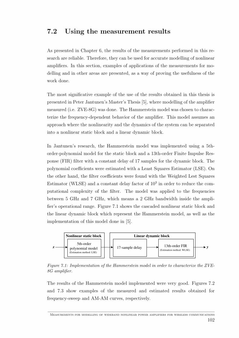
7.2 Using the measurement results
As presented in Chapter 6, the results of the measurements performed in this re-
search are reliable. Therefore, they can be used for accurate modelling of nonlinear
amplifiers. In this section, examples of applications of the measurements for mo-
delling and in other areas are presented, as a way of proving the usefulness of the
work done.
The most significative example of the use of the results obtained in this thesis is
presented in Peter Jantunen’s Master’s Thesis [5], where modelling of the amplifier
measured (i.e. ZVE-8G) was done. The Hammerstein model was chosen to charac-
terize the frequency-dependent behavior of the amplifier. This model assumes an
approach where the nonlinearity and the dynamics of the system can be separated
into a nonlinear static block and a linear dynamic block.
In Jantunen’s research, the Hammerstein model was implemented using a 5th-
order-polynomial model for the static block and a 13th-order Finite Impulse Res-
ponse (FIR) filter with a constant delay of 17 samples for the dynamic block. The
polynomial coefficients were estimated with a Least Squares Estimator (LSE). On
the other hand, the filter coefficients were found with the Weighted Lest Squares
Estimator (WLSE) and a constant delay factor of 103 in order to reduce the com-
putational complexity of the filter. The model was applied to the frequencies
between 5 GHz and 7 GHz, which means a 2 GHz bandwidth inside the ampli-
fier’s operational range. Figure 7.1 shows the cascaded nonlinear static block and
the linear dynamic block which represent the Hammerstein model, as well as the
implementation of this model done in [5].
5th-order
polynomial model (Estimation method: LSE)
17-sample delay 13th-order FIR (Estimation method: WLSE)
Nonlinear static block Linear dynamic block
x y
Figure 7.1: Implementation of the Hammerstein model in order to characterize the ZVE-8G amplifier.
The results of the Hammerstein model implemented were very good. Figures 7.2
and 7.3 show examples of the measured and estimated results obtained for
frequency-sweep and AM-AM curves, respectively.
Measurements for modelling of wideband nonlinear power amplifiers for wireless communications
102
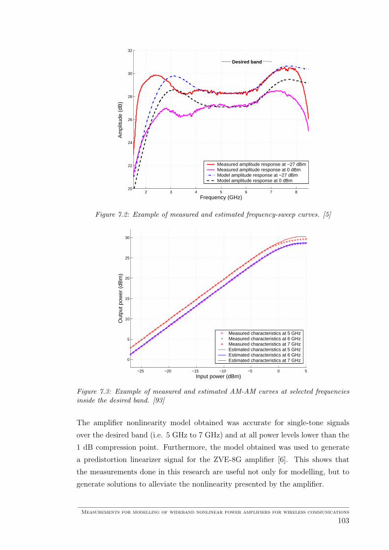
2 3 4 5 6 7 820
22
24
26
28
30
32
Frequency (GHz)
Am
plitu
de (
dB)
Measured amplitude response at −27 dBmMeasured amplitude response at 0 dBmModel amplitude response at −27 dBmModel amplitude response at 0 dBm
Desired band
Figure 7.2: Example of measured and estimated frequency-sweep curves. [5]
−25 −20 −15 −10 −5 0 5
0
5
10
15
20
25
30
Input power (dBm)
Out
put p
ower
(dB
m)
Measured characteristics at 5 GHzMeasured characteristics at 6 GHzMeasured characteristics at 7 GHzEstimated characteristics at 5 GHzEstimated characteristics at 6 GHzEstimated characteristics at 7 GHz
Figure 7.3: Example of measured and estimated AM-AM curves at selected frequenciesinside the desired band. [93]
The amplifier nonlinearity model obtained was accurate for single-tone signals
over the desired band (i.e. 5 GHz to 7 GHz) and at all power levels lower than the
1 dB compression point. Furthermore, the model obtained was used to generate
a predistortion linearizer signal for the ZVE-8G amplifier [6]. This shows that
the measurements done in this research are useful not only for modelling, but to
generate solutions to alleviate the nonlinearity presented by the amplifier.
Measurements for modelling of wideband nonlinear power amplifiers for wireless communications
103
The amplifier modelling topic is widely researched nowadays. Consequently, there
have been several approaches on the way of using measurements similar to the
ones presented in this thesis. For instance, a Wiener-Hammerstein model designed
based on multi-tone measurements of a broad-band RF amplifier [24]; a model for
bandpass nonlinearities based on harmonic measurements [94]; or an approach of
nonlinear spectral regrowth modelling based on measured continuous wave ampli-
fier data [95].
Moreover, measurements of amplifiers are extensively used to prove in a practical
way the theoretical and simulated results of linearization methods, such as a post-
distortion receiver for mobile communications [96] or a third-order intermodulation
reduction method in nonlinear microwave systems [97].
In general, the necessity of representing the nonlinearity of power amplifiers and
linearizers is becoming overwhelming in recent wireless applications, where wide-
band digital modulated signals with high Peak-to-Average Ratio (PAR), such as
third-generation (3G) signals, are used [98]. Therefore, nowadays measurement ap-
plications have the common final aim of improving the efficiency of future wireless
transmissions.
7.3 Summary of the chapter
In this chapter aspects to be considered after performing amplifier measurements
were discussed. First, comments on the possible errors that may have occurred
during the measurements performed in this thesis were given. As previously
commented, high accurate measurements are a difficult task to achieve since many
factors are involved in the process, from which some can be avoided or controlled
but others are inherent to the setup system and to the device under test itself.
Next, the usefulness of measurements similar to the ones presented in this thesis
was analyzed. Measurements of amplifiers were proven to be useful. This fact is
supported by a recent example of the application of the ZVE-8G amplifier measures
obtained in this research on the modelling of the amplifier. Finally, other examples
of the usage of this type of measurements were commented and referred.
Measurements for modelling of wideband nonlinear power amplifiers for wireless communications
104

Chapter 8
Conclusions and future work
This chapter finalizes the work done in this thesis by presenting a brief summary of
the carried out research, the conclusions obtained and recommendations for future
work related to amplifier measurements.
Throughout Chapters 2 and 3, the basic theory about amplifiers was introduced,
including the most common distortion parameters obtained from measurements
using different input signals. Harmonic distortion appearing at frequencies multi-
ple of the fundamental frequency is the main nonlinear effect produced by single-
tone input signals. Moreover, AM-AM and AM-PM characteristic curves respec-
tively show the output amplitude and phase behavior when varying the input
signal. However, it is necessary to perform a frequency-sweep measurement, in
order to represent the memory effects introduced by amplifiers. Furthermore, a
two-tone input signal was used to obtained the intermodulation products in the
output spectrum. The third intermodulation product present in the fundamental
zone is the most important parameter obtained from a two-tone test because it
is the frequency component closest to the fundamental tone and, therefore, it is
difficult to filter out with simple methods. In addition, a multisine signal was
chosen for measuring the effects of a nonlinear amplifier over high peak-to-average
ratio signals.
Chapters 4 and 5 presented the necessary aspects to plan and perform measure-
ments of amplifier nonlinearity. An overview of modelling and estimation methods
was done in order to determine the type of measurements required to characterize
Measurements for modelling of wideband nonlinear power amplifiers for wireless communications
105

the amplifier distortion. Next, the procedure and setup systems to perform single-,
two- and multi-tone signal measurements were presented. Emphasis was made on
the modelling parameters to be obtained from each type of measurement.
The results obtained from performing practical measurements are presented in
Chapter 6. The amplifier used is a Mini-Circuits ZVE-8G wideband high-power
amplifier. Parameters such as the average gain inside the amplifier’s operational
range, the 1 dB compression point and the third intermodulation product were
found with single-tone signal measurements, giving a positive result when com-
pared to the expected values. A two-tone signal was generated and the intermo-
dulation distortion ratio, among other distortion measures, was measured. Finally,
a 300-tone multisine signal was generated. When feeding the amplifier with this
signal the adjacent power channel ratio and the multi-tone intermodulation ratio
were obtained, showing the expected behavior (i.e. higher nonlinear distortion for
higher input levels).
Chapter 7 summarized aspects to be considered after performing amplifier mea-
surements. Comments on the possible errors that may have occurred during the
measurements performed and examples of the usage of the results were given. A re-
cent example of the application of the amplifier measures obtained in this research
on the modelling of the amplifier was described. Finally, complementary infor-
mation needed to fulfil the objective of this research is annexed on Appendices A
to D. This includes the equipment specification, setup systems and processes used,
as well as the full set of results.
The objective of this thesis was to provide the basis to perform accurate measure-
ments of power amplifiers to obtain reliable data for characterizing their nonli-
nearity. The objective was achieved throughout this research with theoretical and
practical work. Next, the main conclusions found in this research are presented.
An extensive variety of parameters can be obtained from amplifier measurements.
In general, it was observed that signals with higher number of tones represent
better the distortion introduced by an amplifier. However, signals with one or two
tones can give an easy-manipulable and clear approximation of the nonlinearity
caused by an amplifier. For instance, it was shown how the frequency-dependent
and frequency-independent behavior of the amplifier can be modelled based on
the AM-AM, AM-PM and frequency-sweep curves obtained from single-tone sig-
Measurements for modelling of wideband nonlinear power amplifiers for wireless communications
106
nal measurements performed in this thesis. Therefore, it is essential to previously
determine the needed parameters for a specific model, in order to better characte-
rize an amplifier.
Moreover, it was determined that highly accurate measurements are a difficult task
to achieve since many aspects are involved in the process. It was found that some
of these factors can be avoided or controlled but others are inherent to the setup
system and to the device under test itself. Therefore, specialized equipment and
careful planning should be considered in order to avoid unnecessary errors and loss
that unavoidably lead to inaccurate results.
Furthermore, the usability of the results obtained from measurements similar to
the ones presented in this thesis was found to be very wide. An example of amplifier
modelling based on measurements done in this research and a literature review on
more applications of measurements in modelling proved this observation. In this
sense, this thesis contribution is summarized into a full set of measurement results,
from which diverse models can be derived.
Finally, there are many more aspects to be considered for future research. Exam-
ples for future work, including some related references, are:
¦ Develop more exact measuring systems. For instance, the three-tone test, which
shows more accurately the effect of adjacent channels in the nonlinear distortion
of an amplifier [99, 100].
¦ Find and perform measuring methods that characterize better the phase distor-
tion and memory effects of amplifiers [101, 102, 103].
¦ Perform multi-tone noise power ratio measurements to analyze in-band distor-
tion caused by an amplifier and make tests with noisy input signals in order to
analyze the effect of amplifier distortion in carrier-to-noise ratio [104, 105, 106].
¦ Analyze the distortion carried by amplifiers in time-domain [107, 108, 109].
¦ Design a predistortion signal, based on a model designed with data obtained
from this measurements and measure its performance with different input signals
(single-, two- and multi-tone) [110, 111].
Measurements for modelling of wideband nonlinear power amplifiers for wireless communications
107
References
[1] Jos, R. Future developments and technology options in cellular phone power
amplifiers: from power amplifier to integrated RF front-end module. In
Proceedings of the 2000 Bipolar/BiCMOS Circuits and Technology Meeting,
MN, USA, 2000. Philips Discrete Semiconductors.
[2] Ahmed, N.; et al. Finite backlog effects on downlink scheduling. Technical
report, Department of Electrical and Computer Engineering. Rice University,
2003.
[3] ACTIX for decisive data. WCDMA radio link engineering basics: lessons
learned from 2G IS-95 CDMA and GSM networks. White paper, 2002.
[4] Costa, E.; et al. Impact of amplifier nonlinearities on OFDM transmission
system performance. IEEE Communications Letters, 2(2), February 1999.
[5] Jantunen, P. Modelling of nonlinear power amplifiers for wireless communi-
cations. Master’s thesis, Helsinki University of Technology, Espoo, Finland,
March 2004.
[6] Cheong, M.; et al. Design of pre-distorters for power ampli-
fiers in future communications systems. In IEEE Nordic Sig-
nal Processing Symposium, NORSIG’04, Espoo, Finland, June 2004.
http://wooster.hut.fi/publications/norsig2004/.
[7] Sedra, A.; et al. Microelectronic circuits. Oxford University Press, New York,
USA, fourth edition, 1998.
[8] Beals, G. Biography of Thomas Alva Edison. Internet: http://www.-
thomasedison.com/biog.htm, 1999.
Measurements for modelling of wideband nonlinear power amplifiers for wireless communications
108
[9] Wolff, C. Radar-basics. Travelling wave tube: physical construction and
functional describing. Internet: http://mitglied.lycos.de/radargrundlagen/-
top-en.html, Germany, 1996-2004.
[10] UltraRF. Application notes: high power solid state circuit design. Internet:
http://www.cree.com/ftp/pub/appnote3.pdf.
[11] Van Fleteren, S. Traveling wave tube vs. solid state amplifiers. Technical
report, Communications and Power Industries (formely Varian Associates),
2000.
[12] Turner, S. D. Reliability advantages of modular solid state power amplifiers
compared to traveling wave tube amplifiers. Technical report, Armed Forces
International, 2003.
[13] Boylestad, R. L.; et al. Electronic devices and circuit theory. Prentice Hall,
Mexico, 6th edition, 1997.
[14] Kenington, P. B. High-linearity RF amplifier design. Artech House, Inc.,
Norwood, MA, USA, 2000.
[15] Sokal, N. O. Class-E RF power amplifiers. QEX, Jaunary/February 2001.
[16] Liang, C-P.; et al. Nonlinear amplifier effects in communications systems.
IEEE Transactions on Microwave Theory and Techniques, 47(8), August
1999.
[17] Andreoli, S.; et al. Nonlinear distortions introduced by amplifier on COFDM
signals. Measurements, effects and compensation techniques. In IEEE
Tyrrhenian Int. Workshop. Itelco R&D and Instituto di Electtronica, Uni-
versita di Perugia, September 1997.
[18] Cheong, M. Y. Constant modulus algorithm based multipath channel es-
timation for OFDM systems with space-time block code. Master’s thesis,
Helsinki University of Technology, Espoo, Finland, November 2002.
[19] Bahai, A.; et al. Multi-carrier digital communications. Theory and applica-
tions of OFDM. Kluwer Academic / Plenum Publishers, NY, USA, 1999.
[20] Maattanen, H.-L. Nonlinear amplification of clipped-filtered multicarrier
signals. Master’s thesis, Helsinki University of Technology, Espoo, Finland,
August 2004.
Measurements for modelling of wideband nonlinear power amplifiers for wireless communications
109
[21] Remley, K. Multisine excitation for ACPR measurements. IEEE MTT-S
Int. Microwave Symp. Dig., June 2003.
[22] Pedro, J.; et al. On the use of multitone techniques for assessing RF compo-
nents’ intermodulation distortion. IEEE Trans. on Microwave Theory and
Techniques, 47(12), December 1999.
[23] Schreurs, D.; et al. Use of multisine signals for efficient behavioural modelling
of RF circuits with short-memory effects. ARFTG 61Philadelphia, June
2003.
[24] Crama, P.; et al. Broad-band measurement and identification of a Wiener-
Hammerstein model for an RF amplifier. 60th ARFTG conference digest,
December 2002.
[25] Sano, M.; et al. Identification of Hammerstein-Wiener system with applica-
tion to compensation for nonlinear distortion. In Proc. SICE Ann. Conf.,
volume 3, August 2002.
[26] Schoukens,J.; et al. Simple methods and insights to deal with nonlinear dis-
tortions in FRF-measurements. Mechanical Systems and Signal Processing,
14(4), 2000.
[27] Braun, M.; et al. Design of minimum crest factor multisinusoidal signals for
plant-friendly identification of nonlinear process systems. In SYSID, CA,
USA, June 2000.
[28] Weiss, M.; et al. Identification of nonlinear cascade systems using paired
multisine signals. IEEE Trans. on Instrumentation and Measurement, 47(1),
February 1998.
[29] Jeruchin, M.; et al. Simulation of communication systems: modelling,
methodology and techniques. KluwerAcademic/Plenum Publishers, NY,
USA, second edition, 2000.
[30] Gutierrez, H.; et al. Nonlinear gain compression in microwave amplifiers
using generalized power-series analysis and transformation of input statistics.
IEEE Trans. Microwave Theory and Tech., 48(10), October 2000.
[31] Guo, Y.; et al. A novel adaptive pre-distorter using LS estimation of SSPA
non-linearity in mobile OFDM systems. In Proc. Int. Symp. on Circuits and
Systems, volume 3, May 2002.
Measurements for modelling of wideband nonlinear power amplifiers for wireless communications
110
[32] Nordsjo, A. An algorithm for adaptive predistortion of certain time-varying
nonlinear high-power amplifiers. In RADAR 2002, October 2002.
[33] Gutierrez, H.; et al. Spectral regrowth in microwave amplifiers using trans-
formation of signal statistics. In IEEE Int. Microwave Symposium Digest,
volume 3, June 1999.
[34] Voros, J. Modeling and identification of wiener systems with two-segment
nonlinearities. IEEE Trans. Control Syst. Tech., 11(2), March 2003.
[35] Saleh, A. Frequency-independent and frequency-dependent nonlinear models
of TWT amplifiers. IEEE Trans. Commun., 29(11), November 1981.
[36] Ghorbani, A.; et al. The effect of solid state power amplifiers (SSPAs)
nonlinearities on MPSK and M-QAM signal transmission. In Proc. Int.
Conf. on Digital Processing of Signals in Communications, September 1991.
[37] Rapp, C. Effects of HPA-nonlinearity on a 4-DPSK/OFDM-signal for a digi-
tal sound broadcasting system. In Proc. of the Second European Conference
on Satellite Communications, Lige, Belgium, October 1991.
[38] White, G.; et al. Modelling of nonlinear distortion in broadband fixed wire-
less access systems. IEEE Electronics Letters., 39(8), April 2003.
[39] Abuelma’atti, M. T. Effect of nonmonotonicity on the intermodulation per-
formance of A/D converters. IEEE Trans. Commun., 33(8), August 1985.
[40] Abuelma’atti, M. T. Frequency-dependent nonlinear quadrature model for
TWT amplifiers. IEEE Trans. Commun., 32(8), August 1984.
[41] Nelles, O. Nonlinear system identification: from classical approaches to neu-
ral network and fuzzy models. Springer–Verlag, Berlin, Germany, 2001.
[42] Bai, E-W. Frequency domain identification of Hammerstein models. IEEE
Trans. Automatic Control, 48(4), April 2003.
[43] Clark, C.; et al. Power amplifier characterization using a two-tone mea-
surement technique. IEEE Trans. Microwave Theory and Techniques, 50(6),
June 2002.
[44] Mathews, J.; et al. Polynomial signal processing. John Wiley & Sons, NY,
USA, 2000.
Measurements for modelling of wideband nonlinear power amplifiers for wireless communications
111

[45] Lesiak, C.; et al. The existence and uniqueness of Volterra series for nonlinear
systems. IEEE Trans. Automatic Control, 23(6), December 1978.
[46] Tummla, M.; et al. Volterra series based modeling and compensation of
nonlinearities in high power amplifiers. In Proc. Int. Conf. on Acoustics,
Speech, and Signal Proc., volume 3, April 1997.
[47] Silva, C.P.; et al. Application of polyspectral techniques to nonlinear model-
ing and compensation. In IEEE MTT-S Internationa Microwave Symposium
Digest, volume 1, AZ, USA, May 2001. Aerosp. Corp., El Segundo.
[48] Kay, S. Fundamentals of statistical signal processing. Prentice Hall Interna-
tional, Inc., NJ, USA, 1993.
[49] Friedlander, B.; et al. The exact Cramer-Rao bound for gaussian autore-
gressive processes. IEEE Trans. Aerospace and Electronic Systems, 25(1),
January 1989.
[50] Peleg, S.; et al. The Cramer-Rao lower bound for signals with constant
amplitude and polynomial phase. IEEE Trans. Signal Processing, 39(3),
March 1991.
[51] Gu, H. Linearization method for finding Cramer-Rao bounds in signal pro-
cessing. IEEE Trans. Signal Processing, 48(2), February 2000.
[52] Stuart, A.; et al. Kendall’s advanced theory of statistics: classical inference
and and the linear model. Oxford University Press, NY, USA, 6 edition,
April 1998.
[53] Rohatgi, V.; et al. An introduction to probability and statistics. Wiley-
Interscience, USA, 2 edition, October 2000.
[54] Eliason, S. Maximum likelihood estimation : logic and practice. SAGE
Publications, USA, August 1993.
[55] Severini, T. Likelihood methods in statistics. Oxford University Press, NY,
USA, January 2001.
[56] Gupta, N.; et al. Computational aspects of maximum likelihood estimation
and reduction in sensitivity function calculations. IEEE Trans. Automatic
Control, 19(6), December 1974.
Measurements for modelling of wideband nonlinear power amplifiers for wireless communications
112

[57] Fang, B. A more direct proof of the minimum variance property of the
linear weighted least-squares estimator. IEEE Trans. Automatic Control,
14(6), December 1969.
[58] Besson, O.; et al. Sinusoidal signals with random amplitude: least-squares
estimators and their statistical analysis. IEEE Trans. Signal Processing,
43(11), November 1995.
[59] Haykin, S. Least-mean-square adaptive filters. Wiley-Interscience, USA,
September 2003.
[60] Laakso, T.; et al. Splitting the unit delay. IEEE Signal Processing Mag.,
13(1), January 1996.
[61] Matyas, L. Generalized method of moments estimation. Cambridge Univer-
sity Press, USA, April 1999.
[62] Powell, J. Notes On method-of-moments estimation. Internet: http://-
emlab.berkeley.edu/users/powell/e241a sp04/mmnotes.pdf. Department of
Economics. University of California, Berkeley.
[63] Bar-Shalom, Y. Estimation with applications to tracking and navigation.
Wiley-Interscience, NY, USA, June 2001.
[64] Pena, D.; et al. A course in time series analysis. Wiley-Interscience, USA,
November 2000.
[65] Ludeman, L. Random processes: filtering, estimation and detection. Wiley-
IEEE Press, NJ, USA, December 2002.
[66] Van Trees, H. Detection, estimation and modulation theory, part I. Wiley-
Interscience, USA, September 2001.
[67] Duda, R. Pattern classification. Wiley-Interscience, USA, 2 edition, October
2000.
[68] Sundresh, T.; et al. Maximum a posteriori estimator for suppression of
interchannel interference in FM receivers. IEEE Trans. Communications,
25(12), December 1977.
[69] Edfors, O.; et al. OFDM channel estimation by singular value decomposition.
IEEE Trans. Communications, 46(7), July 1998.
Measurements for modelling of wideband nonlinear power amplifiers for wireless communications
113

[70] Laverghetta, T. S. Handbook of microwave testing. Artech, USA, 1980.
[71] Shaw, M.; et al. Characterization of a 2 GHz submicron bipolar 60 watt
power transistor with single tone, multi-tone and CDMA signals. In ARFTG
47th, USA, 1996.
[72] Cabot, R. Comparison of nonlinear distortion measurement methods. In
Proceedings of the 11th International AES Conference, 1992.
[73] Schreurs, D.; et al. RF behavioural modelling from multisine measure-
ments: influence of excitation type. In 33rd. European Microwave Conference
(EuMW), Munich, Germany, October 2003.
[74] Agilent Technologies. Introductory operating guide to the Agilent 8780A
vector signal generator, Agilent PN 8780A-1, USA, 1986. Product Note.
[75] LeCroy Corporation, NY, USA. Operator’s manual: LW400 / LW400A/
LW400B WaveStation, April 1999.
[76] Antenna Company Technical Support Team. Intro to SWR. Technical report,
Firestik, AZ, USA, 1996.
[77] Collier, R. J.; et al. Microwave measurements. Peter Peregrinus Ltd., Lon-
don, United Kingdom, second edition, 1989.
[78] Agilent Technologies, USA. Agilent PNA series microwave network analy-
zers: data sheet, September 2002.
[79] Agilent Technologies, USA. Agilent 8560 EC series spectrum analyzers: data
sheet, June 2003.
[80] Lucas, J.R. Basic circuit elements. Technical report, Department of Electri-
cal Engineering, University of Moratuwa, Sri Lanka, November 2001.
[81] Think & Tinker Ltd. The prime source for prototyping equipment and
supplies: Glossary. Internet: http://www.thinktink.com/stack/volumes/-
voliii/reference/glossary.asp#A, July 2004.
[82] Mini-Circuits, NY, USA. Amplifiers, medium high power 50 kHz to 8 GHz:
data sheet.
[83] Agilent Technologies, USA. PNA series network analyzer online help (Dec
2003), December 2003.
Measurements for modelling of wideband nonlinear power amplifiers for wireless communications
114

[84] Katz. E. . Harry Nyquist (biography). Internet: http://www.geocities.com/-
bioelectrochemistry/nyquist.htm, November 2002.
[85] Bennett, W. R. Electrical noise. McGraw Hill Book Company, Inc., New
York, USA, 1960.
[86] Barkley, K. Two-tone IMD measurement techniques. Seven rules to ensure
the best characterization of non-linear RF components. RF test & measure-
ment, June 2001.
[87] Granberg, H. Measuring the intermodulation distortion of linear ampli-
fiers. Motorola semiconductor engineering bulletin. rf application reports,
Motorola Inc., 1993.
[88] Akaiwa, Y. Introduction to digital mobile communication. Wiley-
Interscience, NY, USA, 1st edition, January 1997.
[89] Vuolevi, J.; et al. Distortion in RF power amplifiers. Artech House, Inc.,
MA, USA, 2003.
[90] Naval Air Systems Command. Avionics Department. AIR-4.5 EW Class
Desk. Naval Air Warfare Center. Weapons Division. Avionics Department.
Electronic Warfare Division. Electronic warfare and radar systems engi-
neering handbook. USA., April 1999.
[91] Quick reference guide. Agilent Technologies 8560 E-series and EC-series
spectrum analyzers, USA, November 2000.
[92] Telegdy, A. Extending the dynamic range of RF/microwave intermodulation
measurements by multiple-carrier cancellation. In The 11th IEEE PIMRC
International Symposium, volume 1, London, UK, September 2000.
[93] Jantunen, P.; et al. Measurements and modelling of nonlinear power am-
plifiers. In IEEE Nordic Signal Processing Symposium, NORSIG’04, Espoo,
Finland, June 2004. http://wooster.hut.fi/publications/norsig2004/.
[94] Behravan, A.; et al. A model for bandpass nonlinearities based on harmonic
measurements. In Proceedings of the IEEE Radio and Wireless conference,
MA, USA, August 2003.
Measurements for modelling of wideband nonlinear power amplifiers for wireless communications
115
[95] Van Moer, W.; et al. Measurement-based nonlinear modeling of spectral
regrowth. IEEE Trans. Instrumentation and Measurement, 50(6), December
2001.
[96] Quach, L.; et al. A postdistortion receiver for mobile communications. IEEE
Trans. Vehicular Technology, 42(4), November 1993.
[97] Hu, Y.; et al. A new method of third-order intermodulation reduction in non-
linear microwave systems. IEEE Trans. Microwave Theory and Techniques,
34(2), February 1986.
[98] Boumaiza, S.; et al. Realistic power-amplifiers characterization with appli-
cation to baseband digital predistortion for 3G base stations. IEEE Trans.
Microwave Theory and Techniques, 50(12), December 2002.
[99] Ma, J-G. Effects of the adjacent channels on IP3 of RF amplifiers. Microwave
and Optical Technology Letters. Wiley Periodicals, Inc., 35(1), October 2002.
[100] Vuolevi, J.; et al. Measurement technique for characterizing memory effects
in RF power amplifiers. IEEE Trans. Microwave Theory and Techniques,
49(8), August 2001.
[101] Ghannouchi, F.; et al. Phase distortion measurements for saturated MES-
FETs loaded with arbitrary impedance terminations. In IEEE Instrumen-
tation and Measurement Technology Conference, volume 1, Hamamatsu,
Japan, May 1994. Dept. of Electr. & Comput. Eng., Ecole Polytech. de
Montreal.
[102] Ku, H.; et al. Extraction of accurate behavioral models for power amplifiers
with memory effects using two-tone measurements. In IEEE MTT-S Inter-
national Microwave Symposium Digest, volume 1, WA, USA, June 2002.
[103] Ku, H.; et al. Quantifying memory effects in RF power amplifiers. IEEE
Trans. Microwave Theory and Techniques, 50(12), December 2002.
[104] Upshur, J.; et al. Evaluation of linearity characterization techniques for
multicarrier solid-state power amplifiers. In IEEE MTT-S Symposium on
Technologies for Wireless Applications, BC, Canada, February 1999. COM-
SAT Lab. USA.
Measurements for modelling of wideband nonlinear power amplifiers for wireless communications
116

[105] Mallet, A.; et al. A new satellite repeater amplifier characterization system
for large bandwidth NPR and modulated signals measurements. In IEEE
MTT-S International Microwave Symposium Digest, volume 3, WA, USA,
June 2002. Toulouse Space Center, CNES.
[106] Ku, H.; et al. Prediction of output carrier-to-interference ratios from nonli-
near microwave components driven by arbitrary signals using intrinsic kernel
functions. In IEEE Radio and Wireless Conference, CO, USA, September
2000. Sch. of Electr. & Comput. Eng., Georgia Inst. of Technol.
[107] Clark, C.; et al. Time-domain envelope measurement technique with ap-
plication to wideband power amplifier modeling. IEEE Trans. Microwave
Theory and Techniques, 46(12), December 1998.
[108] Draxler, P.; et al. Time domain characterization of power amplifiers with me-
mory effects. In IEEE MTT-S International Microwave Symposium Digest.
QUALCOMM Inc., June 2003.
[109] Muha, M.; et al. Accurate measurement of wideband modulated signals.
Microwave Journal, 43(6), June 2000.
[110] Meier, I.; et al. Error-feedback for amplifier linearization. In Proceedings
of the 1998 South African Symposium on Communications and Signal Pro-
cessing, Rondebosch, South Africa, September 1998. Dept. of Electr. Eng.,
Stellenbosch Univ.
[111] Bosch, W.; et al. Measurement and simulation of memory effects in predis-
tortion linearizers. IEEE Trans. Microwave Theory and Techniques, 37(12),
December 1989.
Measurements for modelling of wideband nonlinear power amplifiers for wireless communications
117

Appendices
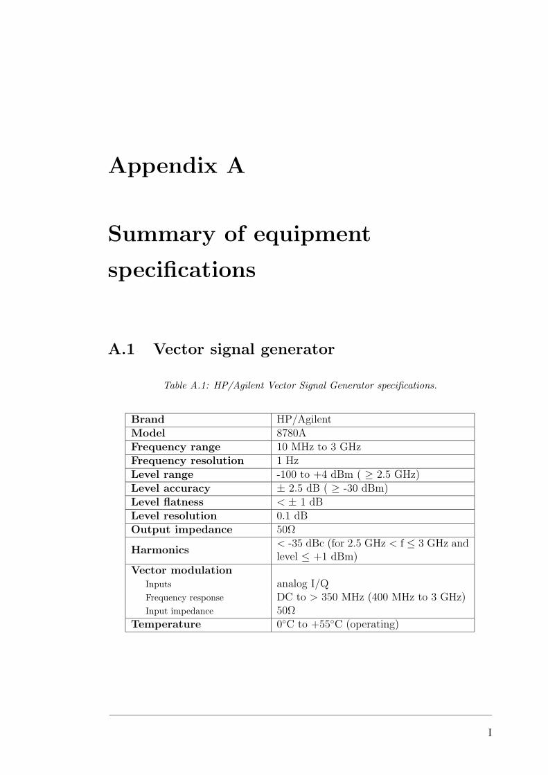
Appendix A
Summary of equipment
specifications
A.1 Vector signal generator
Table A.1: HP/Agilent Vector Signal Generator specifications.
Brand HP/Agilent
Model 8780A
Frequency range 10 MHz to 3 GHz
Frequency resolution 1 Hz
Level range -100 to +4 dBm ( ≥ 2.5 GHz)
Level accuracy ± 2.5 dB ( ≥ -30 dBm)
Level flatness < ± 1 dB
Level resolution 0.1 dB
Output impedance 50Ω
Harmonics< -35 dBc (for 2.5 GHz < f ≤ 3 GHz andlevel ≤ +1 dBm)
Vector modulationInputs analog I/QFrequency response DC to > 350 MHz (400 MHz to 3 GHz)Input impedance 50Ω
Temperature 0C to +55C (operating)
I
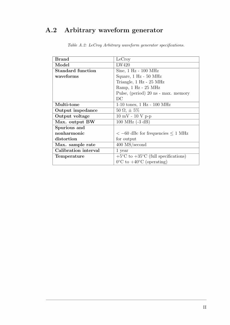
A.2 Arbitrary waveform generator
Table A.2: LeCroy Arbitrary waveform generator specifications.
Brand LeCroy
Model LW420
Standard function Sine, 1 Hz - 100 MHzwaveforms Square, 1 Hz - 50 MHz
Triangle, 1 Hz - 25 MHzRamp, 1 Hz - 25 MHzPulse, (period) 20 ns - max. memoryDC
Multi-tone 1-10 tones, 1 Hz - 100 MHz
Output impedance 50 Ω, ± 5%
Output voltage 10 mV - 10 V p-p
Max. output BW 100 MHz (-3 dB)
Spurious andnonharmonic < −60 dBc for frequencies ≤ 1 MHzdistortion for output
Max. sample rate 400 MS/second
Calibration interval 1 year
Temperature +5C to +35C (full specifications)0C to +40C (operating)
II

A.3 Network analyzer
Table A.3: Agilent Technologies microwave network analyzer specifications.
Brand Agilent Technologies PNA Series
Model E8363A
Frequency range 45 MHz - 40 GHz
Reflection tracking ±1.5 dB (45 MHz to 20 GHz)
Transmission tracking ±2.0 dB (2 MHz to 10 GHz)
Test port outputFrequency resolution 1 HzCW accuracy ±1 ppmPower range -25 to +5 dBm (45 MHz to 10 GHz)Power level accuracy ±1.5 dB (45 MHz to 10 GHz)Power resolution 0.01 dBPhase noise -70 dBc (45 MHz to 10 GHz)Harmonics -23 dBc (for 2nd or 3rd harmonics)Nonharmonic spurious -50 dBc (45 MHz to 20 GHz)
(at nominal output power)
Test port inputNoise floor <-117 dBm
(2 to 10 GHz at 10-Hz IF BW)<-97 dBm(2 to 10 GHz at 1-Hz IF BW)
Receiver compression level <0.6 dB compression at +5 dBm(45 MHz to 20 GHz)
Trace noise magnitude <0.006 dB rms (500 MHz to 20 GHz)Trace noise phase <0.006 rms (500 MHz to 20 GHz)
Measured numberof points 2 to 1601 points per sweep
Temperature 0C to +40C (operating)
III
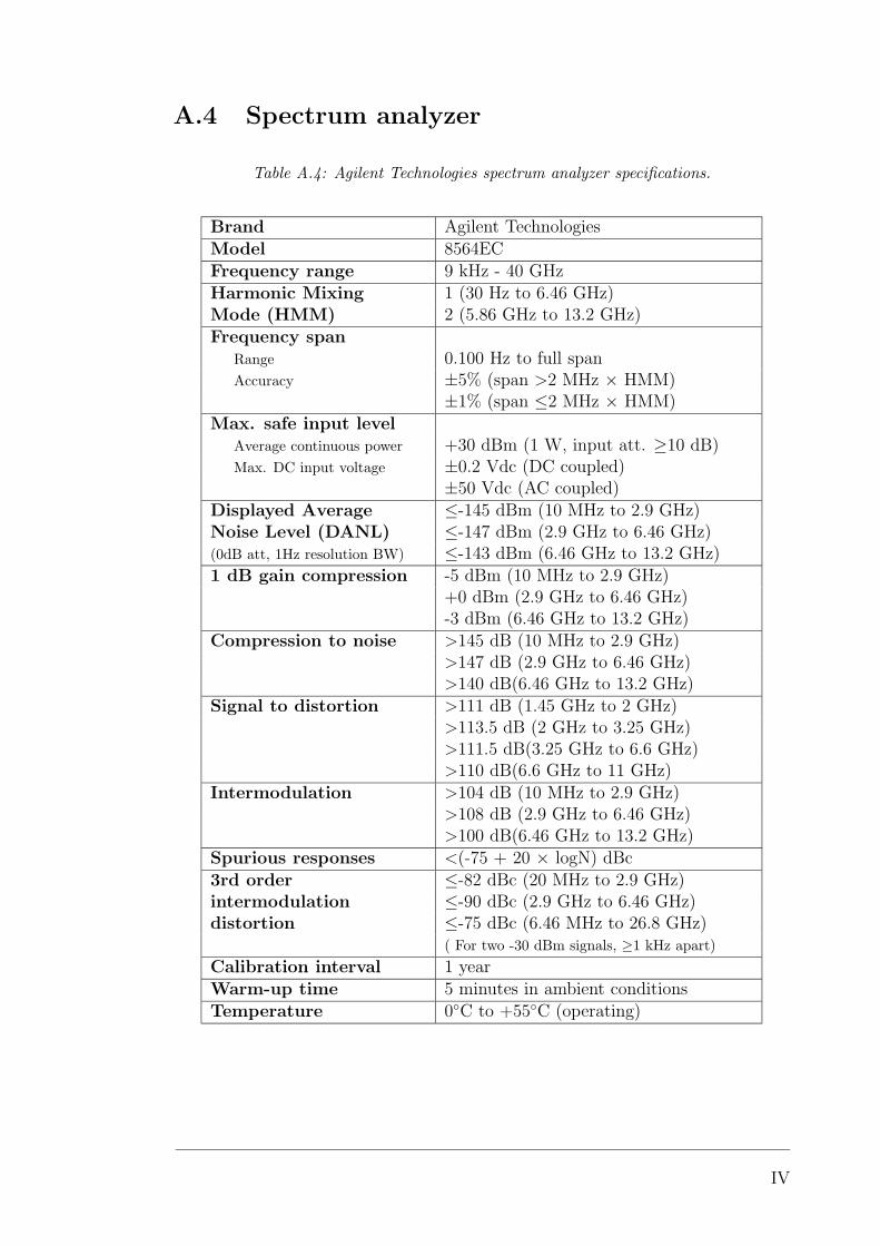
A.4 Spectrum analyzer
Table A.4: Agilent Technologies spectrum analyzer specifications.
Brand Agilent Technologies
Model 8564EC
Frequency range 9 kHz - 40 GHz
Harmonic Mixing 1 (30 Hz to 6.46 GHz)Mode (HMM) 2 (5.86 GHz to 13.2 GHz)
Frequency spanRange 0.100 Hz to full spanAccuracy ±5% (span >2 MHz × HMM)
±1% (span ≤2 MHz × HMM)
Max. safe input levelAverage continuous power +30 dBm (1 W, input att. ≥10 dB)Max. DC input voltage ±0.2 Vdc (DC coupled)
±50 Vdc (AC coupled)
Displayed Average ≤-145 dBm (10 MHz to 2.9 GHz)Noise Level (DANL) ≤-147 dBm (2.9 GHz to 6.46 GHz)(0dB att, 1Hz resolution BW) ≤-143 dBm (6.46 GHz to 13.2 GHz)
1 dB gain compression -5 dBm (10 MHz to 2.9 GHz)+0 dBm (2.9 GHz to 6.46 GHz)-3 dBm (6.46 GHz to 13.2 GHz)
Compression to noise >145 dB (10 MHz to 2.9 GHz)>147 dB (2.9 GHz to 6.46 GHz)>140 dB(6.46 GHz to 13.2 GHz)
Signal to distortion >111 dB (1.45 GHz to 2 GHz)>113.5 dB (2 GHz to 3.25 GHz)>111.5 dB(3.25 GHz to 6.6 GHz)>110 dB(6.6 GHz to 11 GHz)
Intermodulation >104 dB (10 MHz to 2.9 GHz)>108 dB (2.9 GHz to 6.46 GHz)>100 dB(6.46 GHz to 13.2 GHz)
Spurious responses <(-75 + 20 × logN) dBc
3rd order ≤-82 dBc (20 MHz to 2.9 GHz)intermodulation ≤-90 dBc (2.9 GHz to 6.46 GHz)distortion ≤-75 dBc (6.46 MHz to 26.8 GHz)
( For two -30 dBm signals, ≥1 kHz apart)
Calibration interval 1 year
Warm-up time 5 minutes in ambient conditions
Temperature 0C to +55C (operating)
IV
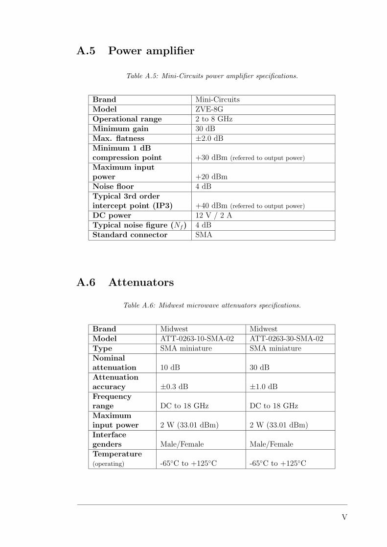
A.5 Power amplifier
Table A.5: Mini-Circuits power amplifier specifications.
Brand Mini-Circuits
Model ZVE-8G
Operational range 2 to 8 GHz
Minimum gain 30 dB
Max. flatness ±2.0 dB
Minimum 1 dBcompression point +30 dBm (referred to output power)
Maximum inputpower +20 dBm
Noise floor 4 dB
Typical 3rd orderintercept point (IP3) +40 dBm (referred to output power)
DC power 12 V / 2 A
Typical noise figure (Nf) 4 dB
Standard connector SMA
A.6 Attenuators
Table A.6: Midwest microwave attenuators specifications.
Brand Midwest Midwest
Model ATT-0263-10-SMA-02 ATT-0263-30-SMA-02
Type SMA miniature SMA miniature
Nominalattenuation 10 dB 30 dB
Attenuationaccuracy ±0.3 dB ±1.0 dB
Frequencyrange DC to 18 GHz DC to 18 GHz
Maximuminput power 2 W (33.01 dBm) 2 W (33.01 dBm)
Interfacegenders Male/Female Male/Female
Temperature(operating) -65C to +125C -65C to +125C
V

Appendix B
Setup systems to perform
measurements
B.1 Setup system to calibrate measuring devices
B.1.1 Setup system to calibrate a network analyzer
Network Analyzer
Adapters
Cables
Internal
generator
output of
Port 1
RF input of
Port 2
Figure B.1: Setup system for calibration of network analyzer.
VI

B.1.2 Setup system to calibrate a spectrum analyzer
Spectrum Analyzer
Adapters
Cables Calibration
output
signal
RF input
Figure B.2: Setup system for calibration of spectrum analyzer.
B.2 Setup system to perform attenuation
measurements
Network Analyzer
Attenuators
Figure B.3: Setup system for attenuation measurements.
VII

B.3 Setup system to perform single-tone signal
measurements
B.3.1 Setup system using a network analyzer
Network Analyzer
OUT IN
Generator Display
Attenuators Amplifier
NWA Logical Interface
(a) Schematic representation
Network Analyzer
Attenuators Amplifier
Cable or adapters
(if needed)
(b) Practical implementation
Figure B.4: Setup system for single-tone signal measurements of amplifiers using anetwork analyzer.
VIII
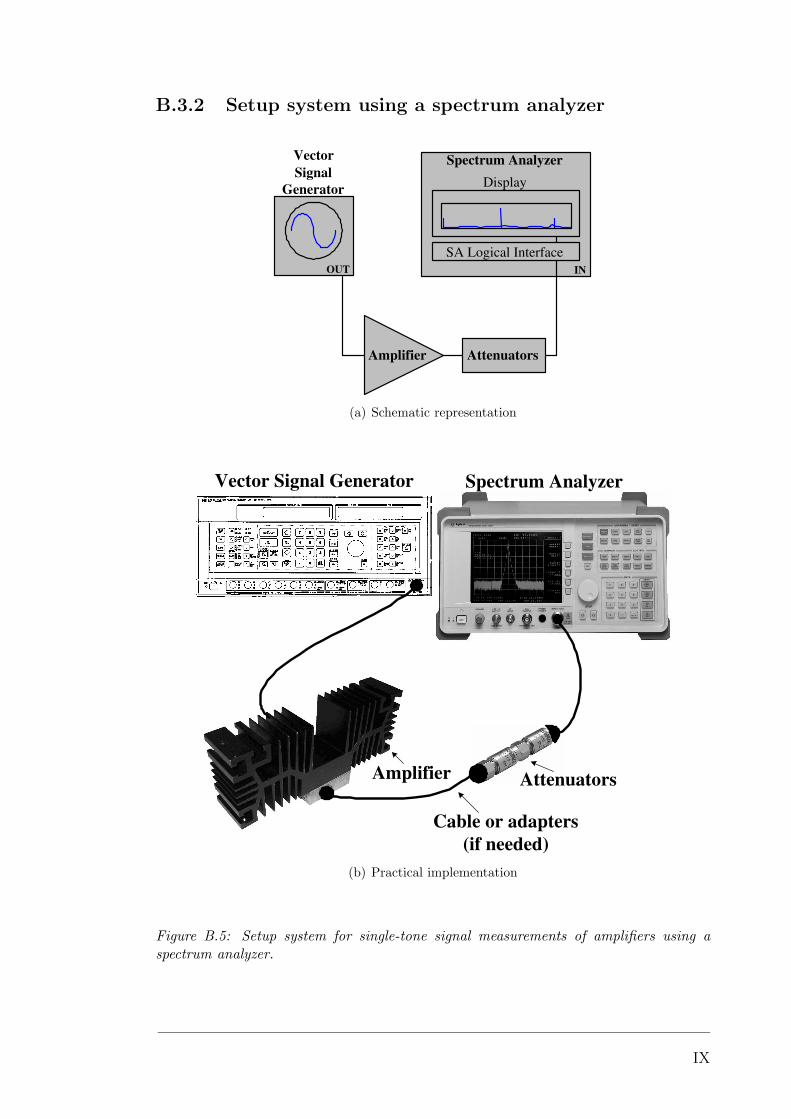
B.3.2 Setup system using a spectrum analyzer
Spectrum Analyzer
IN OUT
Vector
Signal
Generator Display
Attenuators Amplifier
SA Logical Interface
(a) Schematic representation
Spectrum Analyzer
Attenuators Amplifier
Cable or adapters
(if needed)
Vector Signal Generator
(b) Practical implementation
Figure B.5: Setup system for single-tone signal measurements of amplifiers using aspectrum analyzer.
IX
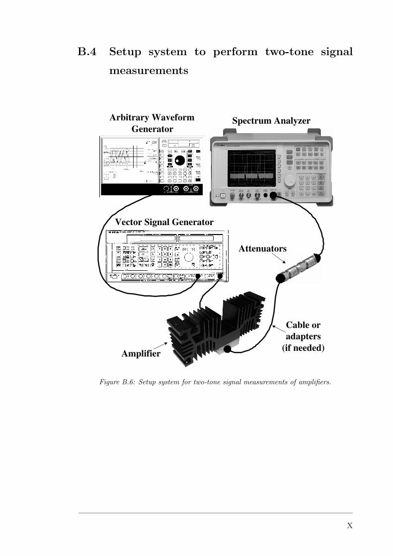
B.4 Setup system to perform two-tone signal
measurements
Spectrum Analyzer
Vector Signal Generator
Arbitrary Waveform
Generator
Attenuators
Amplifier
Cable or
adapters
(if needed)
Figure B.6: Setup system for two-tone signal measurements of amplifiers.
X
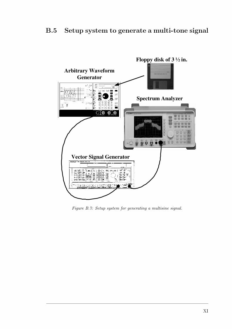
B.5 Setup system to generate a multi-tone signal
Spectrum Analyzer
Arbitrary Waveform
Generator
Floppy disk of 3 ½ in.
Vector Signal Generator
Figure B.7: Setup system for generating a multisine signal.
XI

Appendix C
Processes to perform
measurements
C.1 Process to calibrate measuring devices
C.1.1 Network analyzer calibration
1. Connect calibration system, previously shown in Figure B.1. (Include an
extra connector if necessary)
2. Select from “Channel Setup” panel: Sweep Type → Power Sweep.
3. Select from “Channel Setup” panel: Power.
4. Set “Start Power” at minimum power desired.
5. Set “Stop Power” at maximum power desired.
6. Select from “Channel Setup” panel: Start.
7. Set CW Freq. at the center frequency of the amplifier’s operating range.
8. Select from “Channel Setup” panel: Sweep Type → Linear Frequency.
9. Select from “Channel Setup” panel: Start.
10. Set “Start Frequency” at minimum frequency desired.
11. Select from “Channel Setup” panel: Stop.
12. Set “Stop Frequency” at maximum frequency desired.
13. Select from “Channel Setup” panel: Power.
14. Set “Power Level” at 0 dBm.
XII

15. Check that Power is “ON” (Power ON/off).
16. Select from the main menu bar (at the top of the screen): Sweep → Number
of Points → Custom, and set for the desired number of points to be measured
in the frequency span. Click OK.
17. Select from the main menu bar: Calibration, and set Interpolation “ON”
(Interpolation ON/off).
18. Select from the main menu bar: Calibration → Calibration Wizard.
19. Select “Unguided Calib...” → “Use Mechanical Stds.”
20. Check the box “Create new Cal Set”. Click Next.
21. Select “THRU Response”. Click Next.
22. Click the THRU button (THRU (trans) Por...). Click OK. Click Next. (It
is possible to select to save the Calibration Settings in a specific file and
location in the NWA system. This file can be recalled to get the parameters
just obtained from this calibration.)
The parameters for calibration currently used can be checked at any time by
selecting from the main menu bar: Calibration → Cal-Set, then select the active
CalSet (marked as ∗) and click “Properties”.
C.1.2 Spectrum analyzer calibration
1. Connect calibration system, previously shown in Figure B.2. (Include an
extra connector if necessary)
2. Select from the main panel: Frequency.
3. Set “Center Freq” at the frequency of the calibration signal.
4. Adjust the frequency span if desired by selecting from the main panel: Span
and setting “Span” as desired.
5. Select from “Calibration” panel: Cal → REF LVL ADJ.
6. Use the knob to adjust the peak of the signal to the top of grid.
7. Select “STORE REF LVL” to store the value of the amplitude correction
needed (e.g. zero for no correction).
8. Press “ENTER” from the main panel.
XIII
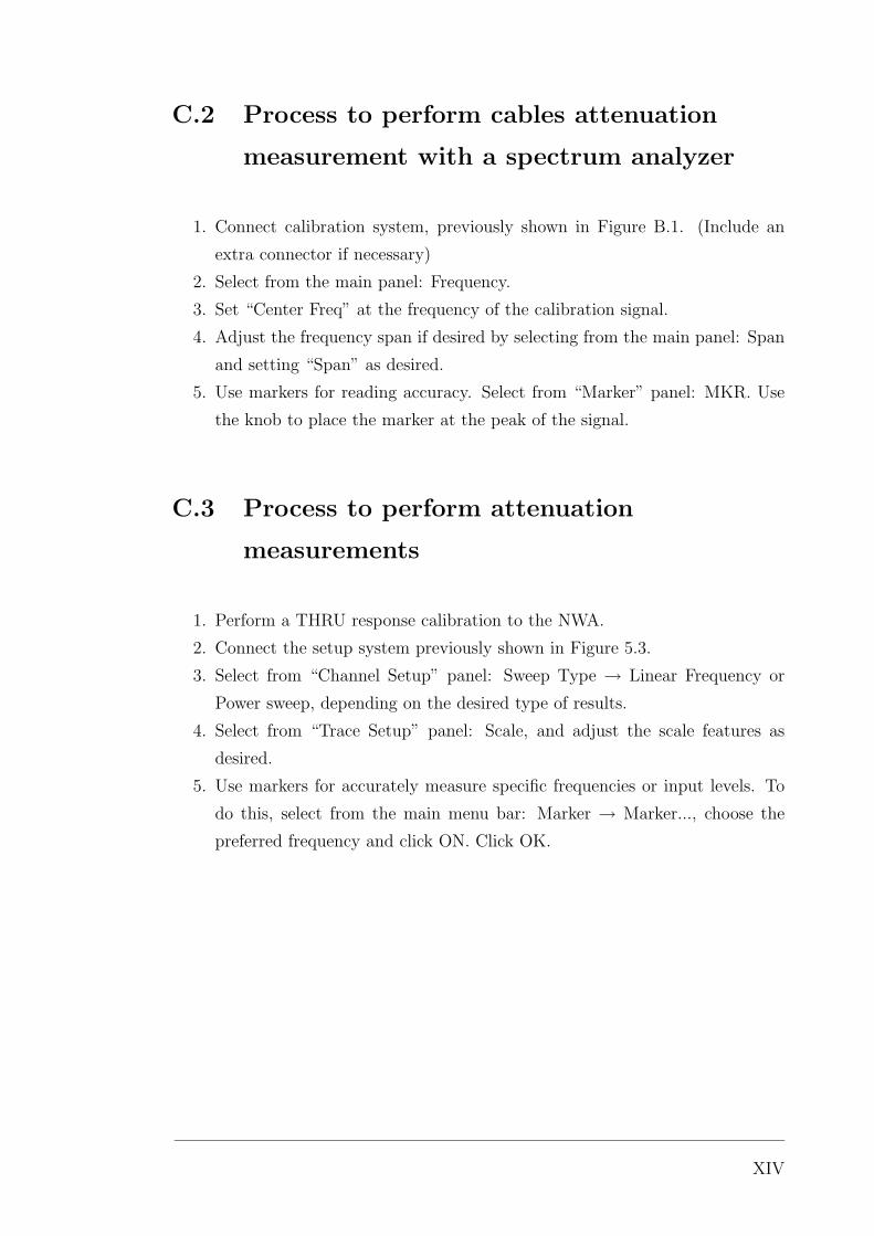
C.2 Process to perform cables attenuation
measurement with a spectrum analyzer
1. Connect calibration system, previously shown in Figure B.1. (Include an
extra connector if necessary)
2. Select from the main panel: Frequency.
3. Set “Center Freq” at the frequency of the calibration signal.
4. Adjust the frequency span if desired by selecting from the main panel: Span
and setting “Span” as desired.
5. Use markers for reading accuracy. Select from “Marker” panel: MKR. Use
the knob to place the marker at the peak of the signal.
C.3 Process to perform attenuation
measurements
1. Perform a THRU response calibration to the NWA.
2. Connect the setup system previously shown in Figure 5.3.
3. Select from “Channel Setup” panel: Sweep Type → Linear Frequency or
Power sweep, depending on the desired type of results.
4. Select from “Trace Setup” panel: Scale, and adjust the scale features as
desired.
5. Use markers for accurately measure specific frequencies or input levels. To
do this, select from the main menu bar: Marker → Marker..., choose the
preferred frequency and click ON. Click OK.
XIV
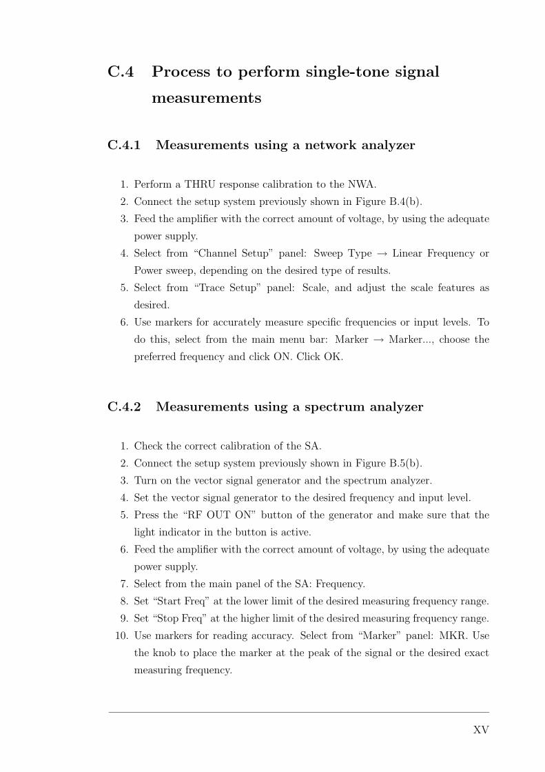
C.4 Process to perform single-tone signal
measurements
C.4.1 Measurements using a network analyzer
1. Perform a THRU response calibration to the NWA.
2. Connect the setup system previously shown in Figure B.4(b).
3. Feed the amplifier with the correct amount of voltage, by using the adequate
power supply.
4. Select from “Channel Setup” panel: Sweep Type → Linear Frequency or
Power sweep, depending on the desired type of results.
5. Select from “Trace Setup” panel: Scale, and adjust the scale features as
desired.
6. Use markers for accurately measure specific frequencies or input levels. To
do this, select from the main menu bar: Marker → Marker..., choose the
preferred frequency and click ON. Click OK.
C.4.2 Measurements using a spectrum analyzer
1. Check the correct calibration of the SA.
2. Connect the setup system previously shown in Figure B.5(b).
3. Turn on the vector signal generator and the spectrum analyzer.
4. Set the vector signal generator to the desired frequency and input level.
5. Press the “RF OUT ON” button of the generator and make sure that the
light indicator in the button is active.
6. Feed the amplifier with the correct amount of voltage, by using the adequate
power supply.
7. Select from the main panel of the SA: Frequency.
8. Set “Start Freq” at the lower limit of the desired measuring frequency range.
9. Set “Stop Freq” at the higher limit of the desired measuring frequency range.
10. Use markers for reading accuracy. Select from “Marker” panel: MKR. Use
the knob to place the marker at the peak of the signal or the desired exact
measuring frequency.
XV
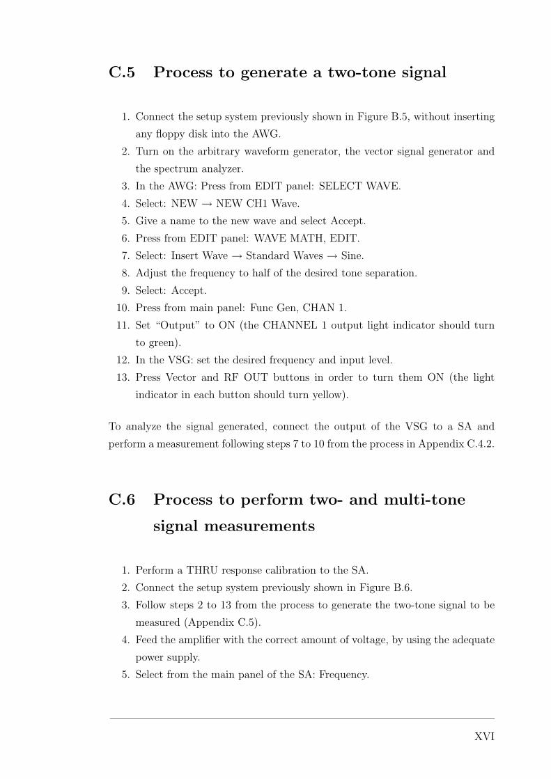
C.5 Process to generate a two-tone signal
1. Connect the setup system previously shown in Figure B.5, without inserting
any floppy disk into the AWG.
2. Turn on the arbitrary waveform generator, the vector signal generator and
the spectrum analyzer.
3. In the AWG: Press from EDIT panel: SELECT WAVE.
4. Select: NEW → NEW CH1 Wave.
5. Give a name to the new wave and select Accept.
6. Press from EDIT panel: WAVE MATH, EDIT.
7. Select: Insert Wave → Standard Waves → Sine.
8. Adjust the frequency to half of the desired tone separation.
9. Select: Accept.
10. Press from main panel: Func Gen, CHAN 1.
11. Set “Output” to ON (the CHANNEL 1 output light indicator should turn
to green).
12. In the VSG: set the desired frequency and input level.
13. Press Vector and RF OUT buttons in order to turn them ON (the light
indicator in each button should turn yellow).
To analyze the signal generated, connect the output of the VSG to a SA and
perform a measurement following steps 7 to 10 from the process in Appendix C.4.2.
C.6 Process to perform two- and multi-tone
signal measurements
1. Perform a THRU response calibration to the SA.
2. Connect the setup system previously shown in Figure B.6.
3. Follow steps 2 to 13 from the process to generate the two-tone signal to be
measured (Appendix C.5).
4. Feed the amplifier with the correct amount of voltage, by using the adequate
power supply.
5. Select from the main panel of the SA: Frequency.
XVI

6. Set “Start Freq” at the lower limit of the desired measuring frequency range.
7. Set “Stop Freq” at the higher limit of the desired measuring frequency range.
8. Use markers for reading accuracy. Select from “Marker” panel: MKR. Use
the knob to place the marker at the peak of the signal or the desired exact
measuring frequency.
C.7 Process to generate a multisine signal
1. Connect the setup system previously shown in Figure B.7.
2. Turn on the arbitrary waveform generator, the vector signal generator and
the spectrum analyzer.
3. Insert the floppy disk containing the file with the multisine data into the
drive of the Arbitrary Waveform Generator (AWG).
4. In the AWG: Press from main panel: PROJECT.
5. Select: Import → What → Matlab.
6. Select: Target File: Import As.
7. Give a name to the new wave and select Accept Name.
8. Make sure that the “Source File” is the desired one and select: Import
(importing the file will take some time, depending on the length of the file).
9. Press from main panel: Func Gen, CHAN 1.
10. Set “Output” to ON (the CHANNEL 1 output light indicator should turn
to green).
11. In the VSG: set the desired frequency and input level.
12. Press Vector and RF OUT buttons in order to turn them ON (the light
indicator in each button should turn yellow).
To analyze the signal generated, connect the output of the VSG to a SA and
perform a measurement following steps 7 to 10 from the process in Appendix C.4.2.
XVII

C.8 Miscellaneous processes
Saving screens in the network analyzer
1. Select from the main menu bar: File → Print to file...
2. Select the location to be saved and write a name for the file.
3. Select from the desired format. (Formats available: bitmap (.bpm), joint
photographic experts group (.jpg) and portable network graphics (.png))
4. Click OK.
Saving data in a file from the network analyzer
1. Select from the main menu bar: File → Save as...
2. Select the location to be saved and write a name for the file.
3. Select Trace format (.s2p), which includes a stimulus response column plus
a real value column and an imaginary value column for each of the four
S-parameters.
4. Click OK.
Using averaging function in the spectrum analyzer
1. Press from control panel: BW
2. Set “VID AVG” to ON.
3. Set the desired average factor (0 to 100) by pressing the desired number of
average factor in the number keypad, followed by pressing “Hz”.
XVIII
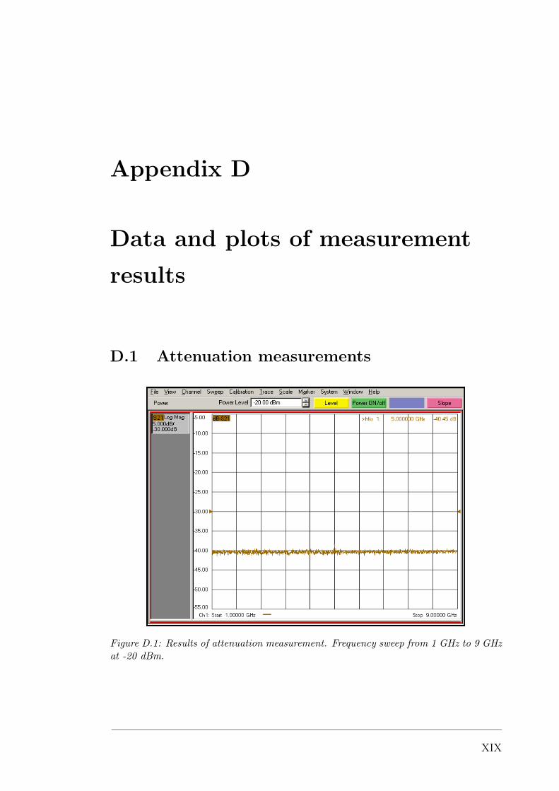
Appendix D
Data and plots of measurement
results
D.1 Attenuation measurements
Figure D.1: Results of attenuation measurement. Frequency sweep from 1 GHz to 9 GHzat -20 dBm.
XIX

Figure D.2: Results of attenuation measurement. Power sweep from -27 dBm to +3 dBmat 2 GHz.
Figure D.3: Results of attenuation measurement. Power sweep from -27 dBm to +3 dBmat 8 GHz.
XX
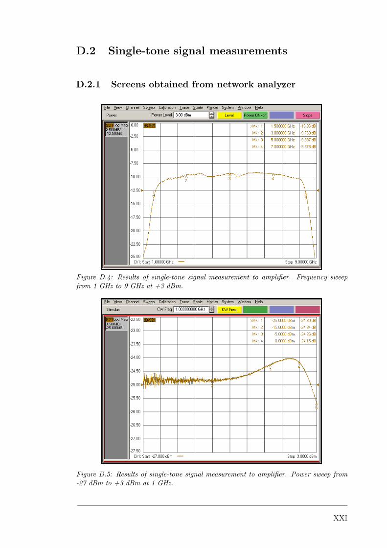
D.2 Single-tone signal measurements
D.2.1 Screens obtained from network analyzer
Figure D.4: Results of single-tone signal measurement to amplifier. Frequency sweepfrom 1 GHz to 9 GHz at +3 dBm.
Figure D.5: Results of single-tone signal measurement to amplifier. Power sweep from-27 dBm to +3 dBm at 1 GHz.
XXI
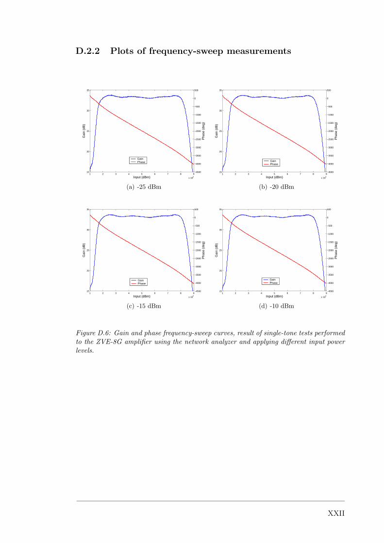
D.2.2 Plots of frequency-sweep measurements
1 2 3 4 5 6 7 8 9
x 109
15
20
25
30
35
Input (dBm)
Gai
n (d
B)
−4500
−4000
−3500
−3000
−2500
−2000
−1500
−1000
−500
0
500
Pha
se (
deg)
GainPhase
(a) -25 dBm
1 2 3 4 5 6 7 8 9
x 109
15
20
25
30
35
Input (dBm)
Gai
n (d
B)
−4500
−4000
−3500
−3000
−2500
−2000
−1500
−1000
−500
0
500
Pha
se (
deg)
GainPhase
(b) -20 dBm
1 2 3 4 5 6 7 8 9
x 109
15
20
25
30
35
Input (dBm)
Gai
n (d
B)
−4500
−4000
−3500
−3000
−2500
−2000
−1500
−1000
−500
0
500
Pha
se (
deg)
GainPhase
(c) -15 dBm
1 2 3 4 5 6 7 8 9
x 109
15
20
25
30
35
Input (dBm)
Gai
n (d
B)
−4500
−4000
−3500
−3000
−2500
−2000
−1500
−1000
−500
0
500
Pha
se (
deg)
GainPhase
(d) -10 dBm
Figure D.6: Gain and phase frequency-sweep curves, result of single-tone tests performedto the ZVE-8G amplifier using the network analyzer and applying different input powerlevels.
XXII
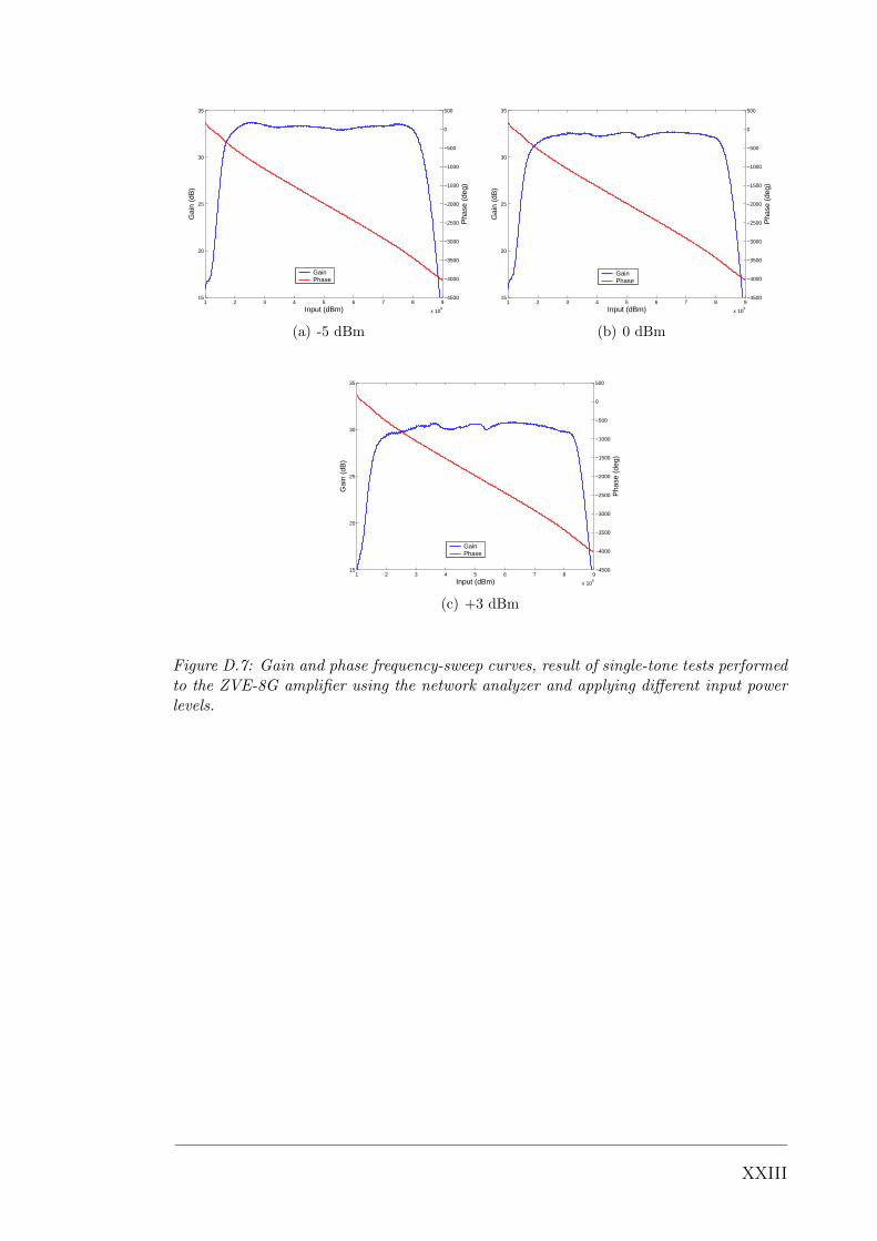
1 2 3 4 5 6 7 8 9
x 109
15
20
25
30
35
Input (dBm)
Gai
n (d
B)
−4500
−4000
−3500
−3000
−2500
−2000
−1500
−1000
−500
0
500
Pha
se (
deg)
GainPhase
(a) -5 dBm
1 2 3 4 5 6 7 8 9
x 109
15
20
25
30
35
Input (dBm)
Gai
n (d
B)
−4500
−4000
−3500
−3000
−2500
−2000
−1500
−1000
−500
0
500
Pha
se (
deg)
GainPhase
(b) 0 dBm
1 2 3 4 5 6 7 8 9
x 109
15
20
25
30
35
Input (dBm)
Gai
n (d
B)
−4500
−4000
−3500
−3000
−2500
−2000
−1500
−1000
−500
0
500
Pha
se (
deg)
GainPhase
(c) +3 dBm
Figure D.7: Gain and phase frequency-sweep curves, result of single-tone tests performedto the ZVE-8G amplifier using the network analyzer and applying different input powerlevels.
XXIII

D.2.3 Plots of power-sweep measurements
−25 −20 −15 −10 −5 0−15
−10
−5
0
5
10
15
20
Input (dBm)
Out
put (
dBm
)
−300
−200
−100
0
100
200
300
Pha
se (
deg)
AM−AMAM−PM
(a) 1 GHz
−25 −20 −15 −10 −5 05
10
15
20
25
30
35
Input (dBm)
Out
put (
dBm
)
−300
−200
−100
0
100
200
300
Pha
se (
deg)
AM−AMAM−PM
(b) 2 GHz
−25 −20 −15 −10 −5 05
10
15
20
25
30
35
Input (dBm)
Out
put (
dBm
)
−300
−200
−100
0
100
200
300
Pha
se (
deg)
AM−AMAM−PM
(c) 3 GHz
−25 −20 −15 −10 −5 05
10
15
20
25
30
35
Input (dBm)
Out
put (
dBm
)
−300
−200
−100
0
100
200
300
Pha
se (
deg)
AM−AMAM−PM
(d) 4 GHz
Figure D.8: Amplitude and phase characteristics obtained from single-tone tests per-formed to the ZVE-8G amplifier using the network analyzer and applying different inputfrequencies.
XXIV

−25 −20 −15 −10 −5 05
10
15
20
25
30
35
Input (dBm)
Out
put (
dBm
)
−300
−200
−100
0
100
200
300
Pha
se (
deg)
AM−AMAM−PM
(a) 5 GHz
−25 −20 −15 −10 −5 05
10
15
20
25
30
35
Input (dBm)
Out
put (
dBm
)
−300
−200
−100
0
100
200
300
Pha
se (
deg)
AM−AMAM−PM
(b) 6 GHz
−25 −20 −15 −10 −5 05
10
15
20
25
30
35
Input (dBm)
Out
put (
dBm
)
−300
−200
−100
0
100
200
300P
hase
(de
g)
AM−AMAM−PM
(c) 7 GHz
−25 −20 −15 −10 −5 05
10
15
20
25
30
35
Input (dBm)
Out
put (
dBm
)
−300
−200
−100
0
100
200
300
Pha
se (
deg)
AM−AMAM−PM
(d) 8 GHz
−25 −20 −15 −10 −5 0
−15
−10
−5
0
5
10
15
Input (dBm)
Out
put (
dBm
)
−300
−200
−100
0
100
200
300
Pha
se (
deg)
AM−AMAM−PM
(e) 9 GHz
Figure D.9: Amplitude and phase characteristics obtained from single-tone tests per-formed to the ZVE-8G amplifier using the network analyzer and applying different inputfrequencies.
XXV

D.2.4 1 dB compression point plots
−10 −8 −6 −4 −2 0 222
24
26
28
30
32
34
36
Input (dBm)
Out
put (
dBm
)
1 dB
−1.16162
30.814
IdealReal
(a) 2 GHz
−10 −8 −6 −4 −2 0 2
24
26
28
30
32
34
36
Input (dBm)
Out
put (
dBm
)
1 dB
−0.192807
32.1504
IdealReal
(b) 4 GHz
−8 −6 −4 −2 0 224
26
28
30
32
34
36
Input (dBm)
Out
put (
dBm
)
1 dB
0.861134
33.0139
IdealReal
(c) 5 GHz
−8 −6 −4 −2 0 224
26
28
30
32
34
36
Input (dBm)
Out
put (
dBm
)1 dB
0.991979
32.9951
IdealReal
(d) 6 GHz
−10 −8 −6 −4 −2 0 224
26
28
30
32
34
36
Input (dBm)
Out
put (
dBm
)
1 dB
0.432303
32.805
IdealReal
(e) 7 GHz
−10 −8 −6 −4 −2 0 2
24
26
28
30
32
34
36
Input (dBm)
Out
put (
dBm
)
1 dB
−0.0125852
32.002
IdealReal
(f) 8 GHz
Figure D.10: 1 dB compression point for ZVE-8G amplifier, calculated for frequenciesmeasured inside the operational band and based on the AM-AM characteristic obtainedfrom the corresponding power-sweep measurement performed with the network analyzer.
XXVI
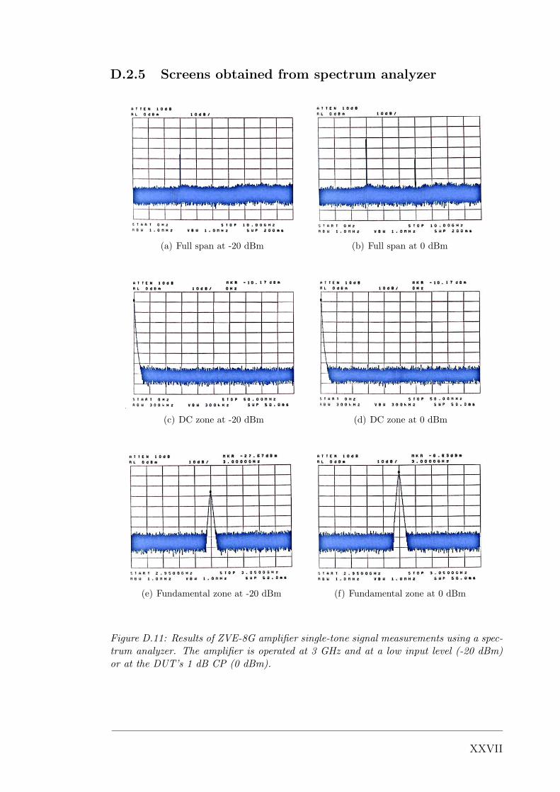
D.2.5 Screens obtained from spectrum analyzer
(a) Full span at -20 dBm (b) Full span at 0 dBm
(c) DC zone at -20 dBm (d) DC zone at 0 dBm
(e) Fundamental zone at -20 dBm (f) Fundamental zone at 0 dBm
Figure D.11: Results of ZVE-8G amplifier single-tone signal measurements using a spec-trum analyzer. The amplifier is operated at 3 GHz and at a low input level (-20 dBm)or at the DUT’s 1 dB CP (0 dBm).
XXVII
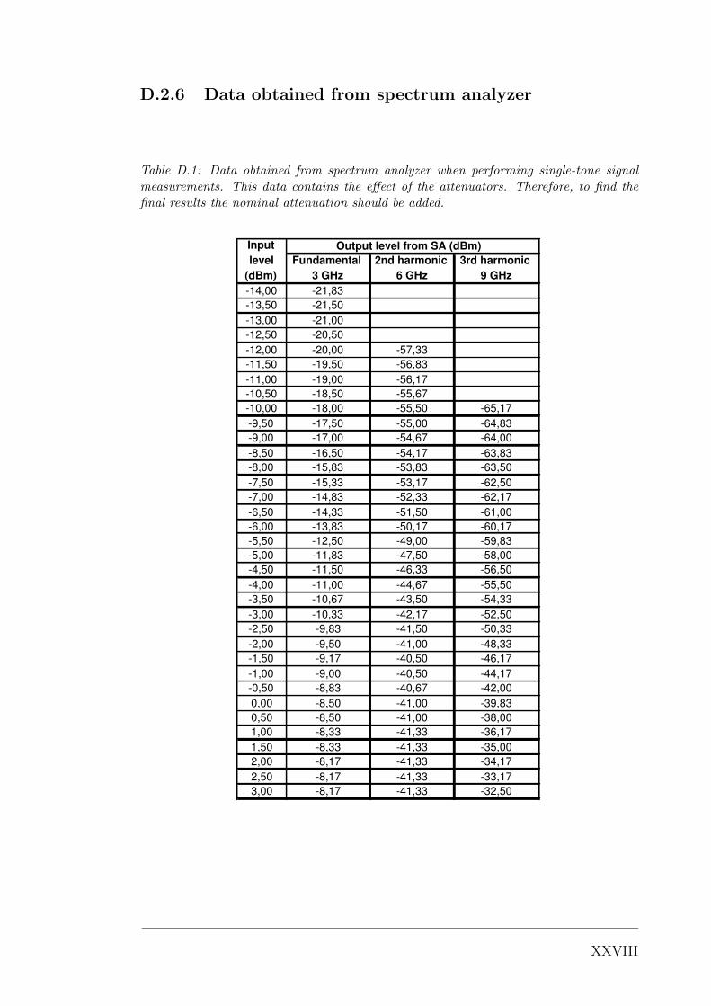
D.2.6 Data obtained from spectrum analyzer
Table D.1: Data obtained from spectrum analyzer when performing single-tone signalmeasurements. This data contains the effect of the attenuators. Therefore, to find thefinal results the nominal attenuation should be added.
Fundamental 2nd harmonic 3rd harmonic
3 GHz 6 GHz 9 GHz
-14,00 -21,83
-13,50 -21,50
-13,00 -21,00
-12,50 -20,50
-12,00 -20,00 -57,33
-11,50 -19,50 -56,83
-11,00 -19,00 -56,17
-10,50 -18,50 -55,67
-10,00 -18,00 -55,50 -65,17
-9,50 -17,50 -55,00 -64,83
-9,00 -17,00 -54,67 -64,00
-8,50 -16,50 -54,17 -63,83
-8,00 -15,83 -53,83 -63,50
-7,50 -15,33 -53,17 -62,50
-7,00 -14,83 -52,33 -62,17
-6,50 -14,33 -51,50 -61,00
-6,00 -13,83 -50,17 -60,17
-5,50 -12,50 -49,00 -59,83
-5,00 -11,83 -47,50 -58,00
-4,50 -11,50 -46,33 -56,50
-4,00 -11,00 -44,67 -55,50
-3,50 -10,67 -43,50 -54,33
-3,00 -10,33 -42,17 -52,50
-2,50 -9,83 -41,50 -50,33
-2,00 -9,50 -41,00 -48,33
-1,50 -9,17 -40,50 -46,17
-1,00 -9,00 -40,50 -44,17
-0,50 -8,83 -40,67 -42,00
0,00 -8,50 -41,00 -39,83
0,50 -8,50 -41,00 -38,00
1,00 -8,33 -41,33 -36,17
1,50 -8,33 -41,33 -35,00
2,00 -8,17 -41,33 -34,17
2,50 -8,17 -41,33 -33,17
3,00 -8,17 -41,33 -32,50
Output level from SA (dBm) Input
level
(dBm)
XXVIII

D.2.7 Plot of fundamental, second harmonic and third
harmonic curves
-30,00
-25,00
-20,00
-15,00
-10,00
-5,00
0,00
5,00
10,00
15,00
20,00
25,00
30,00
35,00
-14,
00
-13,
00
-12,
00
-11,
00
-10,
00
-9,0
0
-8,0
0
-7,0
0
-6,0
0
-5,0
0
-4,0
0
-3,0
0
-2,0
0
-1,0
0
0,00
1,00
2,00
3,00
Input level
Ou
tpu
t le
ve
l
Fundamental
Second harmonic
Third harmonic
Figure D.12: Fundamental, second harmonic and third harmonic curves based on dataobtained from spectrum analyzer when performing single-tone signal measurements. Thedata used for this plot contains the effect of the attenuators. Therefore, to find the finalresults the nominal attenuation should be added.
XXIX

D.3 Two-tone signal measurements
D.3.1 Screens obtained from spectrum analyzer
(a) Full span (b) DC zone
(c) Second harmonic zone (d) Third harmonic zone
Figure D.13: Measurements of the generated two-tone signal obtained with a spectrumanalyzer. The two-tone signal has a center frequency of 3 GHz, tone separation of60 MHz and it is tested at a high input power level equal to the 1 dB CP of the DUT(0 dBm).
XXX
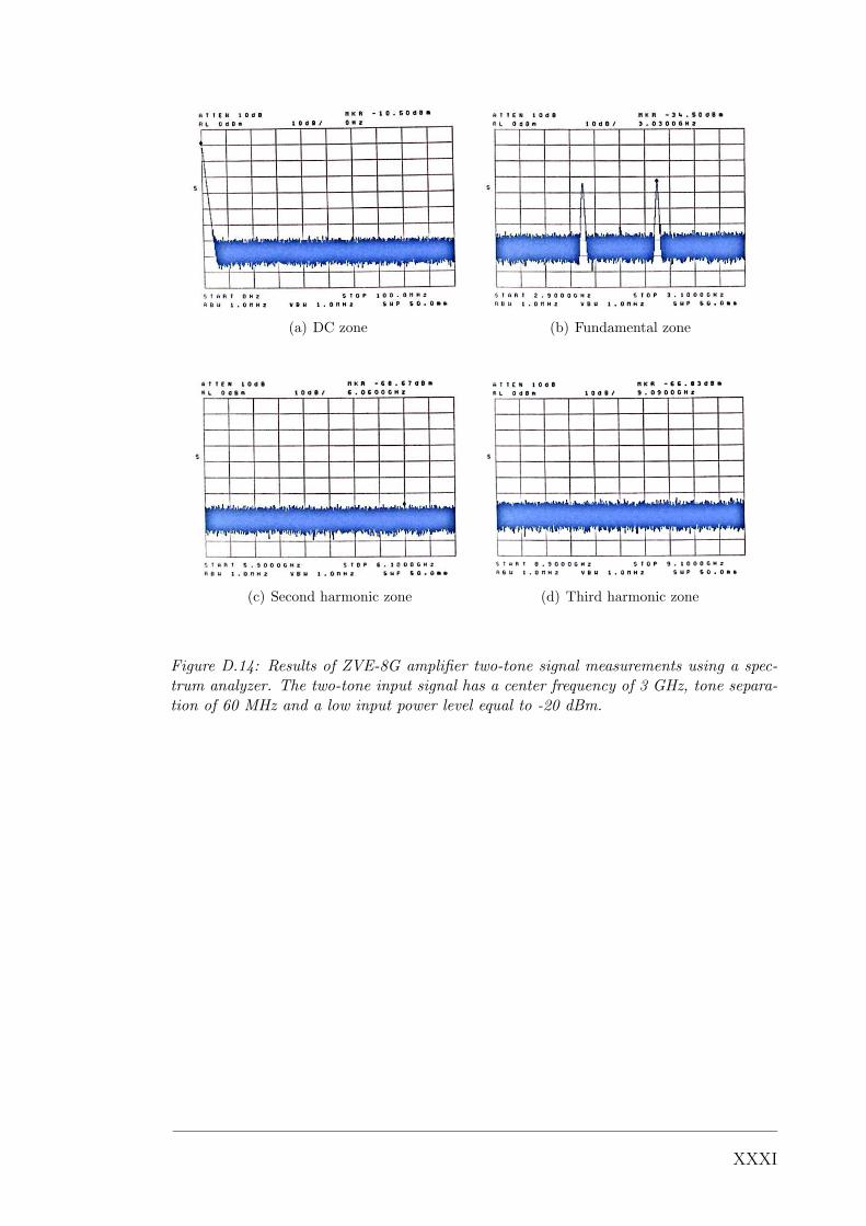
(a) DC zone (b) Fundamental zone
(c) Second harmonic zone (d) Third harmonic zone
Figure D.14: Results of ZVE-8G amplifier two-tone signal measurements using a spec-trum analyzer. The two-tone input signal has a center frequency of 3 GHz, tone separa-tion of 60 MHz and a low input power level equal to -20 dBm.
XXXI
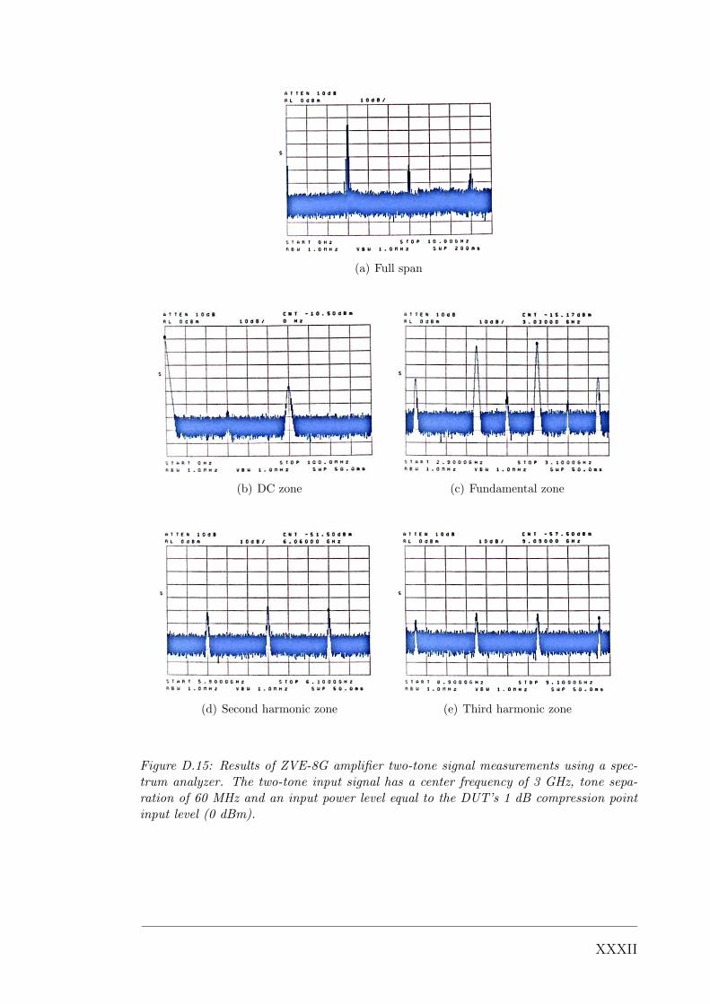
(a) Full span
(b) DC zone (c) Fundamental zone
(d) Second harmonic zone (e) Third harmonic zone
Figure D.15: Results of ZVE-8G amplifier two-tone signal measurements using a spec-trum analyzer. The two-tone input signal has a center frequency of 3 GHz, tone sepa-ration of 60 MHz and an input power level equal to the DUT’s 1 dB compression pointinput level (0 dBm).
XXXII
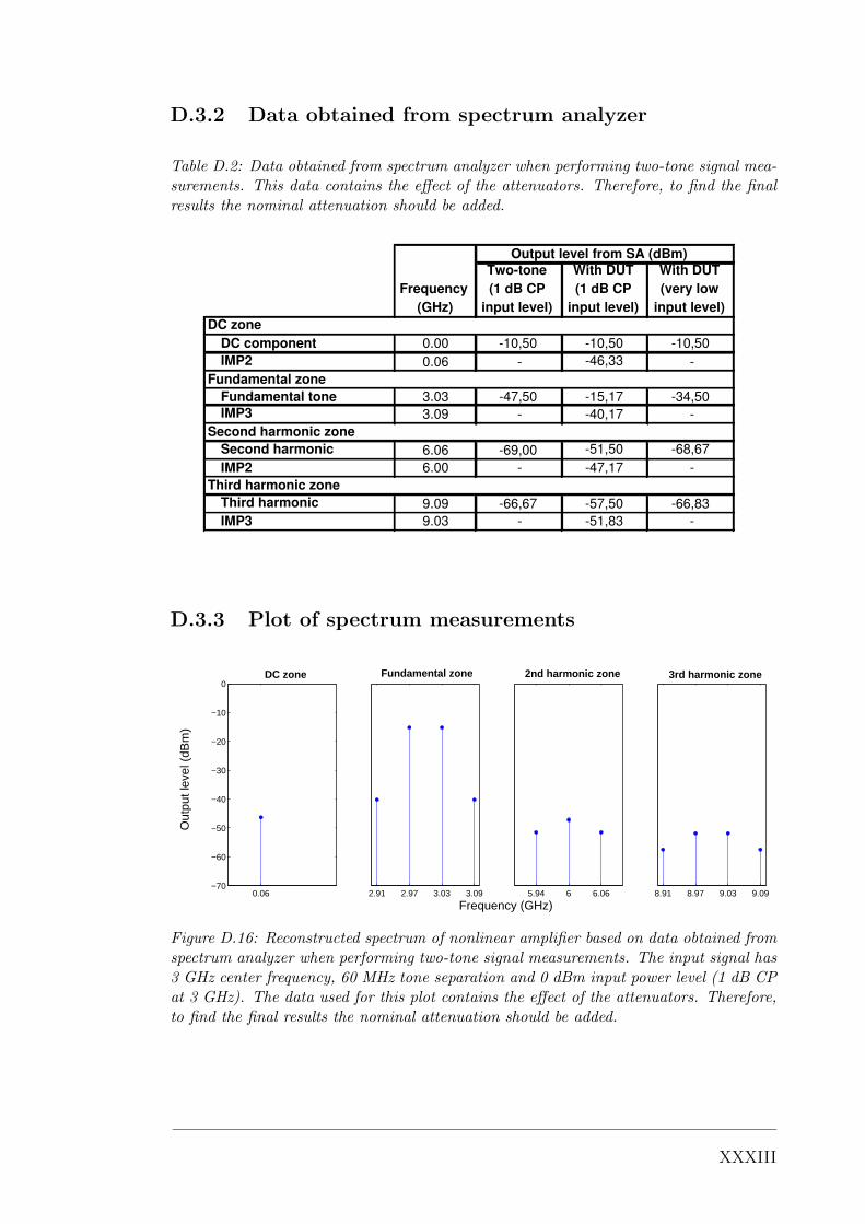
D.3.2 Data obtained from spectrum analyzer
Table D.2: Data obtained from spectrum analyzer when performing two-tone signal mea-surements. This data contains the effect of the attenuators. Therefore, to find the finalresults the nominal attenuation should be added.
DC zone
DC component 0.00 -10,50 -10,50 -10,50
IMP2 0.06 - -46,33 -
Fundamental zone
Fundamental tone 3.03 -47,50 -15,17 -34,50
IMP3 3.09 - -40,17 -
Second harmonic zone
Second harmonic 6.06 -69,00 -51,50 -68,67
IMP2 6.00 - -47,17 -
Third harmonic zone
Third harmonic 9.09 -66,67 -57,50 -66,83
IMP3 9.03 - -51,83 -
Output level from SA (dBm)
Frequency
(GHz)
Two-tone
(1 dB CP
input level)
With DUT
(1 dB CP
input level)
With DUT
(very low
input level)
D.3.3 Plot of spectrum measurements
0.06
0
−10
−20
−30
−40
−50
−60
−70
Out
put l
evel
(dB
m)
2.91 2.97 3.03 3.09 5.94 6 6.06 8.91 8.97 9.03 9.09
Frequency (GHz)
DC zone Fundamental zone 2nd harmonic zone 3rd harmonic zone
Figure D.16: Reconstructed spectrum of nonlinear amplifier based on data obtained fromspectrum analyzer when performing two-tone signal measurements. The input signal has3 GHz center frequency, 60 MHz tone separation and 0 dBm input power level (1 dB CPat 3 GHz). The data used for this plot contains the effect of the attenuators. Therefore,to find the final results the nominal attenuation should be added.
XXXIII

D.4 Multi-tone signal measurements
D.4.1 Screens obtained from spectrum analyzer
(a) Full span
(b) Fundamental zone (c) Fundamental zone (zoom)
(d) Second harmonic zone (e) Third harmonic zone
Figure D.17: Measurements of the generated multisine signal obtained with a spectrumanalyzer. The multisine signal has a center frequency of 3 GHz, bandwidth of 60 MHzand it is tested at a high input power level equal to the 1 dB CP of the DUT (0 dBm).
XXXIV

(a) Fundamental zone (b) Fundamental zone (zoom)
(c) Second harmonic zone (d) Third harmonic zone
Figure D.18: Results of ZVE-8G amplifier multi-tone signal measurements using a spec-trum analyzer. The multisine input signal has a center frequency of 3 GHz, bandwidthof 60 MHz and a low input power level equal to -20 dBm.
XXXV
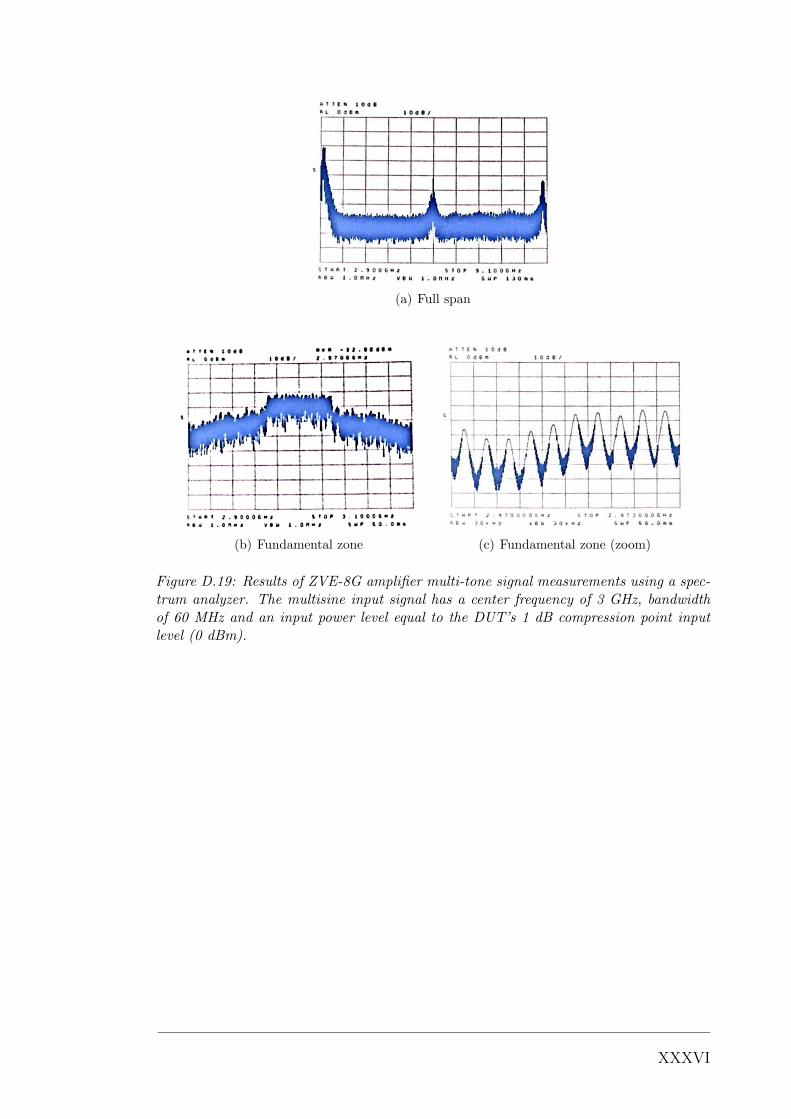
(a) Full span
(b) Fundamental zone (c) Fundamental zone (zoom)
Figure D.19: Results of ZVE-8G amplifier multi-tone signal measurements using a spec-trum analyzer. The multisine input signal has a center frequency of 3 GHz, bandwidthof 60 MHz and an input power level equal to the DUT’s 1 dB compression point inputlevel (0 dBm).
XXXVI
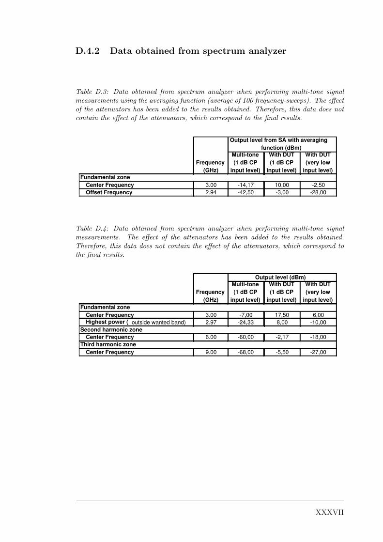
D.4.2 Data obtained from spectrum analyzer
Table D.3: Data obtained from spectrum analyzer when performing multi-tone signalmeasurements using the averaging function (average of 100 frequency-sweeps). The effectof the attenuators has been added to the results obtained. Therefore, this data does notcontain the effect of the attenuators, which correspond to the final results.
Fundamental zone
Center Frequency 3.00 -14,17 10,00 -2,50
Offset Frequency 2.94 -42,50 -3,00 -28,00
Frequency
(GHz)
Output level from SA with averaging
function (dBm)
Multi-tone
(1 dB CP
input level)
With DUT
(1 dB CP
input level)
With DUT
(very low
input level)
Table D.4: Data obtained from spectrum analyzer when performing multi-tone signalmeasurements. The effect of the attenuators has been added to the results obtained.Therefore, this data does not contain the effect of the attenuators, which correspond tothe final results.
Fundamental zone
Center Frequency 3.00 -7,00 17,50 6,00
Highest power ( outside wanted band) 2.97 -24,33 8,00 -10,00
Second harmonic zone
Center Frequency 6.00 -60,00 -2,17 -18,00
Third harmonic zone
Center Frequency 9.00 -68,00 -5,50 -27,00
Frequency
(GHz)
Output level (dBm)
Multi-tone
(1 dB CP
input level)
With DUT
(1 dB CP
input level)
With DUT
(very low
input level)
XXXVII


