
NPS-SP-12-001
NAVAL POSTGRADUATE
SCHOOL
MONTEREY, CALIFORNIA
MODAL TESTING OF THE NPSAT1 ENGINEERING
DEVELOPMENT UNIT
by
Sajoscha Rahn
July 2012
Approved for public release; distribution unlimited.

i
THIS PAGE INTENTIONALLY LEFT BLANK

i
REPORT DOCUMENTATION PAGE Form Approved OMB No. 0704-0188
Public reporting burden for this collection of information is estimated to average 1 hour per response, including the time for reviewing instructions, searching existing data sources, gathering and maintaining the data needed, and completing and reviewing this collection of information. Send comments regarding this burden estimate or any other aspect of this collection of information, including suggestions for reducing this burden to Department of Defense, Washington Headquarters Services, Directorate for Information Operations and Reports (0704-0188), 1215 Jefferson Davis Highway, Suite 1204, Arlington, VA 22202-4302. Respondents should be aware that notwithstanding any other provision of law, no person shall be subject to any penalty for failing to comply with a collection of information if it does not display a currently valid OMB control number. PLEASE DO NOT RETURN YOUR FORM TO THE ABOVE ADDRESS. 1. REPORT DATE (DD-MM-YYYY) 28-09-2012
2. REPORT TYPE Technical Report
3. DATES COVERED (From-To)
4. TITLE AND SUBTITLE Modal Testing of the NPSAT1 Engineering Development Unit
5a. CONTRACT NUMBER 5b. GRANT NUMBER 5c.PROGRAM ELEMENT NUMBER
6. AUTHOR(S) Sajoscha Rahn
5d. PROJECT NUMBER 5e. TASK NUMBER 5f. WORK UNIT NUMBER
7. PERFORMING ORGANIZATION NAME(S) AND ADDRESS(ES) Naval Postgraduate School Monterey, CA
8.PERFORMING ORGANIZATION REPORT NUMBER NPS-SP-12-001
9. SPONSORING / MONITORING AGENCY NAME(S) AND ADDRESS(ES)
10.SPONSOR/MONITOR’S ACRONYM(S)
11.SPONSOR/MONITOR’S REPORT NUMBER(S)
12. DISTRIBUTION / AVAILABILITY STATEMENT Approved for public release; distribution unlimited 13. SUPPLEMENTARY NOTES The views expressed in this thesis are those of the author and do not reflect the official policy or position of the Department of Defense or the U.S. Government. 14. ABSTRACT The purpose of this thesis is to validate a finite element model of the small satellite NPSAT1. A modal test of this satellite will be conducted and the results will be correlated to the FEM simulation results. Furthermore, this thesis provides an overview of modal parameter extraction techniques and the theories behind them. Impact testing is chosen to obtain the data. In the end, the FEM is found to be inaccurate and suggestions are presented for improvements. 15. SUBJECT TERMS 16. SECURITY CLASSIFICATION OF: 17.
LIMITATION OF ABSTRACT
UU
18. NUMBER OF PAGES
8
19a.NAME OF RESPONSIBLE PERSON Dan Sakoda a. REPORT
UNCLASSIFIED b. ABSTRACT UNCLASSIFIED
c. THIS PAGE UNCLASSIFIED 19b. TELEPHONE NUMBER
(include area code) 831-656-3198
Standard Form 298 (Rev. 8-98) Prescribed by ANSI Std. Z39.18

ii
THIS PAGE INTENTIONALLY LEFT BLANK

iii
NAVAL POSTGRADUATE SCHOOL Monterey, California 93943-5000
Daniel T. Oliver Leonard A. Ferrari President Executive Vice President and Provost The report entitled “Modal Testing of the NPSAT1 Engineering Development Unit” was prepared for the Naval Postgraduate School Space Systems Academic Group. Further distribution of all or part of this report is authorized. This report was prepared by: Sajoscha Rahn, Lt. z. S, German Navy Reviewed by: Released by: Rudolf Panholzer, Jeffrey D. Paduan Chairman Vice President and Space Systems Academic Group Dean of Research

iv
THIS PAGE INTENTIONALLY LEFT BLANK

v
ABSTRACT
The purpose of this thesis is to validate a finite element model of the small
satellite NPSAT1. A modal test of this satellite will be conducted and the results
will be correlated to the FEM simulation results. Furthermore, this thesis provides
an overview of modal parameter extraction techniques and the theories behind
them. Impact testing is chosen to obtain the data. In the end, the FEM is found to
be inaccurate and suggestions are presented for improvements.

vi
THIS PAGE INTENTIONALLY LEFT BLANK

vii
DECLARATION
I hereby declare that this thesis has been created by myself using only the
named sources and supplementary equipment.
ERKLÄRUNG
Hiermit erkläre ich, dass die vorliegende Master Arbeit von mir selbstständig und
nur unter Verwendung der angegebenen Quellen und Hilfsmittel angefertigt
wurde.
Monterey, 01. August 2012
Sajoscha Rahn, Lt. z. S.

viii
THIS PAGE INTENTIONALLY LEFT BLANK

ix
TABLE OF CONTENTS
I. INTRODUCTION .................................................................................................. 1 II. THEORY OF MODAL ANALYSIS ....................................................................... 3
A. BASIC CHECK OF DATA ........................................................................ 3 1. Low-frequency asymptotes ......................................................... 3 2. Mode Indicator Functions (MIFs) ................................................ 4
B. PARAMETER EXTRACTION .................................................................. 6 1. SDOF Modal Analysis Methods .................................................. 7
a) Peak-Picking Method .................................................... 8 b) Circle-Fit Method ........................................................... 9 c) Residual Terms ............................................................ 11
2. MDOF Modal Analysis Methods ................................................ 13 a) Complex Exponential Method .................................... 13 b) Rational Fraction Polynomial Method ....................... 16
C. CORRELATING TEST RESULTS AND SIMULATION RESULTS ....... 19 1. Frequency Response Assurance Criterion .............................. 19 2. Modal Assurance Criterion ........................................................ 19
III. MODAL TESTING OF NPSAT1 ....................................................................... 23 A. TEST SETUP ......................................................................................... 23 B. MEASUREMENTS ................................................................................. 24 C. MODAL ANALYSIS ............................................................................... 25
1. Peak-Picking Method on NPSAT1 Data .................................... 25 2. Circle Fit Analysis of NPSAT1 ................................................... 27 3. Complex Exponential Analysis of NPSAT1 in Frequency
Domain .................................................................................... 30 4. Rational Fraction Polynomial Analysis of NPSAT1 ................ 32
IV. CONCLUSION AND OUTLOOK ...................................................................... 37 V. LIST OF REFERENCES ................................................................................... 41

x
THIS PAGE INTENTIONALLY LEFT BLANK

xi
LIST OF FIGURES
Figure 1: Expanded View of NPSAT1 ........................................................................ 2 Figure 2: Complex Mode Indicator Function (CMIF) .................................................. 5 Figure 3: Multivariate Mode Indicator Function (MMIF) .............................................. 6 Figure 4: Nyquist plot of FRF .................................................................................... 10 Figure 5: Example of Stability Diagram .................................................................... 16 Figure 6: Example of Stability Diagram MIF Overlay ................................................ 17 Figure 7: Example of Frequency Shift ...................................................................... 18 Figure 8: Example of 3D and 2D Presentation of MAC ............................................ 21 Figure 9: Test Setup Free Boundary Conditions and Computer Model .................... 24 Figure 10: Fixed Accelerometers .............................................................................. 24 Figure 11: FRF Ref: 123X-; Res: 11X+ .................................................................... 26 Figure 12: Circle Fit Nyquist Plot Response 11X+ Reference 123X- ....................... 28 Figure 13: Circle Fit Single Mode Curve Fit .............................................................. 28 Figure 14: 3D Animation of Mode 14 Using Circle Fit Method ................................. 29 Figure 15: Complex Exponential Mode Selection Z-Reference ................................ 31 Figure 16: Stability Diagram RFP Global X-Reference ............................................ 33 Figure 17: Cluster Diagram RFP Local X-Reference ............................................... 34 Figure 18: Point Mobility FRF Ref: 123X- ................................................................. 37 Figure 19: MAC Simulation vs. RFP local X-Reference ........................................... 38 Figure 20: 3D MAC Simulation vs. RFP local X-Reference ...................................... 38

xii
THIS PAGE INTENTIONALLY LEFT BLANK

xiii
LIST OF TABLES
Table 1: Example of Numerical Presentation of MAC .............................................. 21 Table 2: Mode Table Using Peak-Picking Method ................................................... 27 Table 3: Circle-Fit Results ........................................................................................ 30 Table 4: Modal Parameters Using Complex Exponential Technique ....................... 32 Table 5: Mode Table using RFP Global Solution ..................................................... 33 Table 6: Mode Table Using RFP Local Solution ....................................................... 35

xiv
THIS PAGE INTENTIONALLY LEFT BLANK

xv
NOTATION
[…] matrix
{…} vector
[…]T transpose of matrix
[…]H Hermitian (transpose complex conjugate) of matrix
[…]* complex conjugate of matrix
!!"! modal constant
!!"(!) individual frequency response function element between coordinates j and k (response at j due to excitation at k)
ℎ!"(!) individual impulse response function element between coordinates j and k (response at j due to excitation at k)
i −1
m number of included modes
N total number of modes
!!" ! dynamic compliance or receptance
! viscous damping
! structural damping
! mode shape
! frequency of vibration in Hz
!! natural frequency of rth mode
1
I. INTRODUCTION
This thesis presents the results of a modal test and analysis of the
engineering development unit (EDU) of the NPSAT1 satellite. Furthermore, a
finite element model is examined and correlated to the test-results. In addition,
we will explore the theory of several parameter extraction techniques.
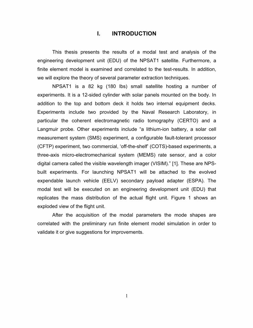
NPSAT1 is a 82 kg (180 lbs) small satellite hosting a number of
experiments. It is a 12-sided cylinder with solar panels mounted on the body. In
addition to the top and bottom deck it holds two internal equipment decks.
Experiments include two provided by the Naval Research Laboratory, in
particular the coherent electromagnetic radio tomography (CERTO) and a
Langmuir probe. Other experiments include “a lithium-ion battery, a solar cell
measurement system (SMS) experiment, a configurable fault-tolerant processor
(CFTP) experiment, two commercial, ‘off-the-shelf’ (COTS)-based experiments, a
three-axis micro-electromechanical system (MEMS) rate sensor, and a color
digital camera called the visible wavelength imager (VISIM).” [1]. These are NPS-
built experiments. For launching NPSAT1 will be attached to the evolved
expendable launch vehicle (EELV) secondary payload adapter (ESPA). The
modal test will be executed on an engineering development unit (EDU) that
replicates the mass distribution of the actual flight unit. Figure 1 shows an
exploded view of the flight unit.
After the acquisition of the modal parameters the mode shapes are
correlated with the preliminary run finite element model simulation in order to
validate it or give suggestions for improvements.
2
Figure 1: Expanded View of NPSAT1

3
II. THEORY OF MODAL ANALYSIS
This chapter describes the complex process of analyzing the data
acquired from modal testing. We will illuminate several different procedures to
extract modal parameters from that data and present some useful tools
developed for this purpose. Furthermore, we will examine the role of correlating
test results with simulated results more closely. It is understood that this
theoretical chapter only accounts for methods used in the experimental section.
This chapter does not present a complete theoretical overview of all possible
methods used in modal analysis today.
A. BASIC CHECK OF DATA
Although preliminary checking of data represents just a crude procedure, it
can be considered a crucial step in modal analysis. The goal of preliminary
checking the data is simply to ensure the acquired FRFs are good enough to be
analyzed. This prevents wasting time and effort on data that subsequently turns
out to be bad data.
1. Low-frequency asymptotes
A simple way to ascertain that the intended boundary conditions have
been achieved is to have a close look at the low-frequency behavior of the FRF.
Using a log-log plot of the FRF, we take a look at the very low frequencies below
the first resonance, because this region correlates to the support conditions
chosen for the test.
In case of a grounded structure, we should see a stiffness-like
characteristic, which means that the FRF approaches a stiffness line
asymptotically at the lowest frequencies. The magnitude should correspond to
that of the static stiffness of the structure.

4
Conversely, in case of a freely supported structure, we should see a
mass-like behavior. However, in practice, there will generally be some rigid body
modes in case of a freely supported structure, interrupting the mass-like trend.
Deviations from this behavior may stem from data not extending far
enough into the lower frequencies or from the intended support conditions not
having been achieved necessitating the test-setup to be revised.
2. Mode Indicator Functions (MIFs)
With the increase of automation, mode indicator functions have been
developed in order to identify natural frequencies more easily, especially in case
of multiple references. In general, test data consist of an n x p Matrix with n being
the number of measurement degrees of freedom (DOFs) and p being the number
of excitation or reference DOFs. Usually, n will be a relatively large number and p
will be 3 or 4. Overall, the principle behind MIFs is an eigenvalue or singular
value decomposition analysis of the FRF-Matrix. A few different MIFs exist and in
this chapter the two commonly used will be examined. Different versions of MIF
employ different formulations leading either to eigenvalue decomposition or
singular value decomposition (SVD). However, both are closely related since the
singular values of a rectangular Matrix [A] are the square root of the eigenvalues
of a square matrix [A]H[A].
Possibly, the most widely used MIF is the Complex Mode Indicator
Function (CMIF). It is defined as a SVD of the FRF-matrix [H(ω)] [2]:
!(!) !×! = !(!) !×! Σ(ω) !×! !(!) !×!! (2.1.
!"#$(!) !×! = Σ(ω) !×!! Σ(ω) !×! (2.2.
The FRF-matrix is decomposed into a matrix of left singular values [U] and
right singular values [V] as well as a rectangular matrix of singular values [Σ], all
of which are frequency dependent. The mode indicator values are provided by
the squares of the singular values and usually plotted on a logarithmic scale. As
5
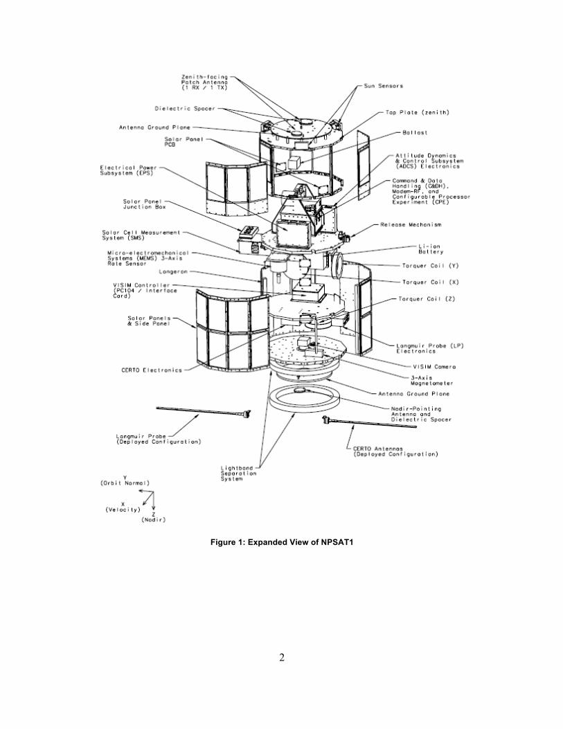
Figure 2 shows, natural frequencies are indicated by large values of the first
CMIF (peaks), and multiple modes can be detected by use of second and third
order CMIF.
Figure 2: Complex Mode Indicator Function (CMIF)
In case of a multiple mode, the second or even third MIF would show a
peak at the same frequency. Additionally, the left singular vector !(!!)
provides an approximation of mode shape for each frequency ωr and the right
singular vector !(!!) provides an approximation of force patterns.
The other common MIF is the Multivariate Mode Indicator Function
(MMIF). This visualization is essentially an eigenvalue decomposition of the FRF-
matrix and solves the problem in equation (2.3).
! ! !! ! ! + ! !
! ! ! ! = ! !! ! ! ! (2.3.
The FRF-matrix has been split up into real [HR] and imaginary [HI] parts.
The solution to this problem is found by identifying the smallest eigenvalue λmin
and corresponding force-eigenvector !!"# . Plotting the solution results in a

6
graph similar to Figure 3. It can be observed that the MMIF identifies natural
frequencies by minima in the graph.
Figure 3: Multivariate Mode Indicator Function (MMIF)
MIFs are very helpful for estimating natural frequencies and validating
acquired data. In connection with parameter extraction techniques, described in
the next section, they truly become powerful tools.
B. PARAMETER EXTRACTION
One purpose of modal analysis is to extract the modal parameters of a
given structure in order to generate the mode shapes and possibly correlating the
results to a previously run simulation. Generally speaking, the analyst can
choose between single degree of freedom (SDOF) methods and multi degree of
freedom (MDOF) methods, however, the test structure more or less dictates
which method to use in order to achieve reasonable results. In this section,
several SDOF and MDOF methods will be presented and their strength and

7
weaknesses will be outlined. This serves the purpose to allow better assessment
of the results obtained by the modal analysis described in the following chapter.
1. SDOF Modal Analysis Methods
The SDOF-approach has been used since the early days of modal testing.
Only in recent times has it been replaced by the more globally working MDOF
methods, although even today the SDOF-approach offers some advantages and
should not be regarded as outdated. In addition it should be noted that the title of
these methods do not refer to the actual degrees of freedom of the tested
structure, but rather that only one resonance is considered at a time. Naturally,
this implies a limitation of the SDOF methods, the major one being that its
accuracy decreases significantly for closely spaced modes. Moreover, this
method is quite a time-consuming task and requires a great amount of user
interaction. Despite its limitations, this method proved to be valuable especially
as a preliminary analysis for quick estimations of the structure’s behavior. Ewins
even states, “that no large-scale modal test should be permitted to proceed until
some preliminary SDOF analyses have been performed” [2].
As we have already seen, SDOF methods rely on the fact that a single
mode dominates the behavior of the structure in the vicinity of a resonance.
Therefore, after [2], we can simplify the algebraic expression of receptance
αjk(ω):
!!"(!) =!!"!
!!! − !! + !!!!!!
!
!!!
(2.4.
First, it is rewritten as
!!" ! =!!"!
!!! − !! + !!!!!!+
!!!!
!!! − !! + !!!!!!
!
!!!!!
(2.5.

8
Now, considering the assumption that in the vicinity of the natural
frequency of mode r, the second term becomes independent of frequency ω and
thus the sum is simplified to the modal constant rBjk. The term for receptance
may now be simplified as:
!!" ! !≃!! ≅!!"!
!!! − !! + !!!!!!+ !!"! (2.6.
This simplification, however, does not diminish the importance of the other
existing modes, but rather simplifies their effect to a constant value, which is
easier to deal with. In fact, the other modes often do have a significant effect.
a) Peak-Picking Method
One of the most straightforward methods is the so-called ‘peak-picking’
method. This method assumes any effect from other modes can be neglected
and that the total response is due to the local mode. Naturally, this method works
reasonably well for structures that exhibit well-separated modes.
[2] describes the method as follows: The first step in ‘peak-picking’ is to
detect the peaks on the FRF plot. One maximum is then taken as natural
frequency ωr of that mode. Next, the corresponding value on the ordinate |Ĥ| is
noted. Following, the ‘half-power points’ are determined as the corresponding
frequencies to !! , which are referred to as ωb and ωa , while !! < !! < !!.
Subsequently, the damping is estimated from formula (2.7).
!! =
!!! − !!!
2!!!= 2!!
(2.7)
Last, the modal constant can be determined by
9
!! = ! !!!!! (2.8)
It is obvious that this method relies heavily on the accuracy of the
maximum FRF level, however, these measurements usually do not provide great
accuracy, since most measurement errors occur in the vicinity of a resonance.
Furthermore, only real modal constants can be estimated by this method. The
other primary limitation is that the single-mode assumption is not strictly correct.
Even if the modes are well separated, the neighboring modes have a significant
influence on the response of the mode in question.
b) Circle-Fit Method
The circle-fit method uses the Nyquist plot of the frequency response data.
For detailed description of the Nyquist plot the reader is referred to chapter 2 in
[2]. In summary, the Nyquist plot produces circle-like curves, which ideally, with
the appropriate parameters would create an exact circle. Depending on the
damping model (viscous or structural) the formulas differ, however the procedure
stays the same. In this case the structural model is chosen and thus we will be
using the receptance form of FRF.
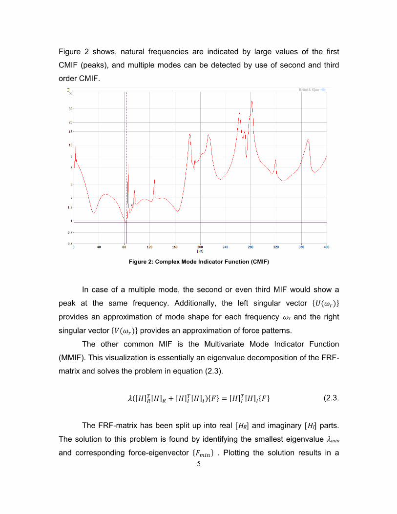
Since the only effect of the modal constant rAjk is to scale the size of the
circle, the basic function for the receptance plot can be used:
! =1
!!! 1− !!!
!+ !!!
(2.9)
In the complex plane, equation (2.9) produces a plot shown in Figure 4.

10
Figure 4: Nyquist plot of FRF
After some algebra, we can obtain the following expression, the reciprocal
of which is the rate of sweep of the locus around the circle.
!!!
!Θ =−!!!!! 1− !
!!! !
2!!! (2.10)
Equation (2.10) reaches the maximum value when = !! , which can be
shown by further differentiation. In this case the damping can be calculated using
equation (2.10). Another technique to acquire the damping is by using two
specific points on the circle ωb and ωa , while !! < !! < !!. The damping
estimates can be obtained from formula (2.11)
!! =
!!! − !!!
!!! !"# Θ!2 + !"# Θ!
2
(2.11)
11
The procedure itself consists of five steps. During the first step, points are
selected for the analysis, either automatically or by the operator. Care should be
taken not to choose points that are influenced by other modes and, ideally, the
selection should encompass 270° of the circle. Furthermore, the range should
not be limited excessively since inaccuracies of the measurements would
become more pronounced. In the end [2] recommends to pick at least six points.
The second step consists of finding a circle-fit for the chosen points. This
is done by means of least-squares deviation. After the specification of the center
and radius, a quality factor is determined, which derives from the mean square
deviation of the selected points from the circle. Generally, an error of 1-2% is
acceptable.
Now the natural frequency is located in the third step and the correlating
damping is obtained. The natural frequency is computed numerically by
practically constructing lines from the center of the circle to a succession of
points around the resonance curve. The angles between those lines are noted
and the rate of sweep is then estimated. From this rate the natural frequency can
be identified.
Step 4 is taken to verify and refine the damping estimates. A set of
damping estimates is calculated using equation (2.11). Now, either a mean value
is computed and taken as the damping for this mode or the values can be
examined individually. Ideally, the damping should be the same, however a
deviation of 4-5% represents a good analysis. To obtain the modal constant we
can now use equation (2.6).
c) Residual Terms
Concluding the SDOF-section, it is essential to introduce the concept of
residual terms. Since it is usually necessary to limit the range of interest in modal
analysis, the residual terms take into account the modes out of range.
When applying the SDOF curve-fit for a series of succeeding modes, a
problem usually occurs when working with the extracted parameters. After the
12
identification of the modes, a construction of a ‘theoretical’ curve that represents
these modes is often desired. However, the regenerated curve is usually a bad
fit, when compared to actual measurements, and this is due to the effect of out-
of-bound modes. Therefore, it is necessary to take modes out of range into
consideration.
For a regenerated FRF curve for the modal series from mode m1 to m2 we
use an equation of the type
!!" ! =!!"!
!!! − !! + !!!!!!
!!
!!!!
(2.12)
The deviation can be seen clearly, when we look at the equation for the
measured data, which accounts for the first mode and the highest mode N, when
it is rewritten as equation (2.14).
!!" ! =!!"!
!!! − !! + !!!!!!
!
!!!
(2.13)
!!" ! = +!!!!
!!!
+!!
!!!!
!!"!
!!! − !! + !!!!!!
!
!!!!!!
(2.14)
The first term represents the lower frequencies and approximates to a
mass-like behavior. The second term relates to the actual modes in the range of
interest, and the third term relates to the higher frequencies, which approximates
to a stiffness effect. Thus, equation (2.14) rewrites as
!!" ! ≅ −1
!!!!"!+
!!"!
!!! − !! + !!!!!!+
1!!"!
!!
!!!!
(2.15)

13
where !!"! and !!"! are the residual mass and stiffness for that FRF.
Naturally, if we extend or limit the range of analysis the residual terms have to be
recalculated.
2. MDOF Modal Analysis Methods
As mentioned earlier, there are some situations for which the SDOF
assumption is inappropriate. This is the case when the structure is extremely
lightly damped or when its modes are closely spaced. The solution is to extract
several modes’ parameters simultaneously in one process. Naturally, this
process is a more complex one and requires an elaborate mathematical
understanding. For the detailed mathematical derivation, the reader is referred to
chapter 4 of [2]. Before continuing to the two MDOF techniques that shall be
discussed, the reader is advised that the idea of residual terms also applies to
MDOF methods.
a) Complex Exponential Method
The complex exponential method as implemented in NX I-deas, is a
MDOF technique that is based on a curve-fitting process in the time-domain. Its
main advantage is that it does not rely on estimates of modal parameters as
starting points. However, it is limited to the use of only one reference location.
For a consideration of multiple references at once, the polyreference method,
which evolved from the complex exponential technique, should be employed [3].
In the first step, we obtain the Impulse Response Function (IRF) via an
Inverse Fourier Transform of the receptance FRF, which leads to an exponential
expression of the IRF:
ℎ!" ! = !!!"!!!!!!
!!!
; !! = −!!!! + !!!! (2.16)
For simplification purposes, we shall change the following notation:

14
!!!" = !! ; !!!!! = !! (2.17)
Note that since the measured FRF usually a discrete function of equally
spaced intervals of frequencies, the IRF also becomes a discrete function of
equally spaced time intervals (Δ! = 1 Δ!). Following this notation, we receive
this system of equations for q samples:
ℎ! = !! + !! +⋯+ !!!ℎ! = !!!! + !!!! +⋯+ !!!!!!ℎ! =⋮
ℎ! =
!!!!! + !!!!! +⋯+ !!!! !!!⋮
!!!!! + !!
!!! +⋯+ !!!! !!!
(2.18)
Now let the number of samples q exceed 4N and we use equation (2.18)
to set up an eigenvalue problem, the solution to which will be the complex natural
frequencies contained in Vr. In order to obtain this solution we introduce
coefficient βi, which eventually leads to the following polynomial:
!! + !!! + !!!! +⋯+ !!!! = 0 (2.19)
We shall now seek the values of the β coefficients to determine the roots
of (2.19) V1, V2, …, Vq which represent the natural frequencies. In order to do so
we let ! ≡ 2! and thus the problem
!!!!! = 0 !"# ! = 1,… ,2!!!
!!!
(2.20)
results in equation (2.21) to be solved.
15
ℎ! ℎ! ℎ! … ℎ!!!!!!!!⋮
= −ℎ!! (2.21)
This process is repeated with a different set of IRF data, always
overlapping for all but one. Thus, the second problem would look like:
ℎ! ℎ! ℎ! … ℎ!!!!!!⋮
= −ℎ!!!! (2.22)
Eventually, this results in a set of 2N linear equations, which can then be
solved for β:
! = − ℎ !! ℎ (2.23)
After having obtained the coefficient β we can now determine the values
V1, V2,…, V2N (2.19) and thus are able to determine the natural frequencies using
(2.17). Furthermore, we may determine the modal constants using equation
(2.24).
! ! = ℎ (2.24)
The complex exponential method is used in the following manner. First, an
estimate for the number of degrees of freedom is made and based upon this the
analysis mentioned above is performed. Subsequently, the extracted modal
parameters are used to create a regenerated FRF, which in turn is compared to
the original measurements. Now, the error between the artificial and the real
curve is computed. This process is then repeated several times, each time using
a different initial estimate of the degrees of freedom. Eventually, as the estimate
of the DOFs approaches the value of the actual DOFs, the error should diminish.
Thus, the modal parameters can be plotted in a so-called stability diagram as
Figure 5 shows. If the initial DOFs estimate is higher than the actual DOFs,
computational modes are created. Generally, they can be identified by their

16
unusually high damping or small modal constants. The stability diagram plots the
results of each iteration (right-hand side axis) and assigns different symbols for
different kind of stabilization:
• stable mode (red diamond)
• vector stable (blue triangle)
• frequency stable (green X)
• damping stable (pink asterisk)
• new mode (cyan cross)
• computational mode (usually filtered, because undesirable)
Figure 5: Example of Stability Diagram
b) Rational Fraction Polynomial Method
The most widely used MDOF frequency domain method is the rational
fraction polynomial method (RFP). It is an advancement of the non-linear least-
squares method and in contrast to its parent, method uses a rational fraction FRF
expression. The advantage the RFP method has over its predecessor is, that the
curve-fitting problem can be formulated as a set of linear equations and thus
allows for a matrix solution.
17
Theoretically, this set of linear equations allows for the solution of every
unknown parameter. However, the RFP method presumes the order of the mode
to be known, when it usually is not and is one of the parameters that are to be
extracted. Therefore, an iteration process is implemented using different values
for the mode order and comparing the results. This leads to the calculation of
genuine modes as well as so called computational or fictional modes. In principle
a mode that repeats after several iterations and is persistent, is most likely a
genuine mode. Modes that vary excessively and occur sporadically throughout
the iteration process are most likely computational modes. Usually, the results of
the iteration process are plotted in a stability diagram (Figure 5) and the analyst
can choose the modes that appear to be the best fit. Modern analysis software
also provides an automatic selection feature. It is at this point, that the MIF come
into action as a powerful tool. In order to help the operator with his/her selection,
the stability diagram can be overlaid with a MIF, so that the modes can be
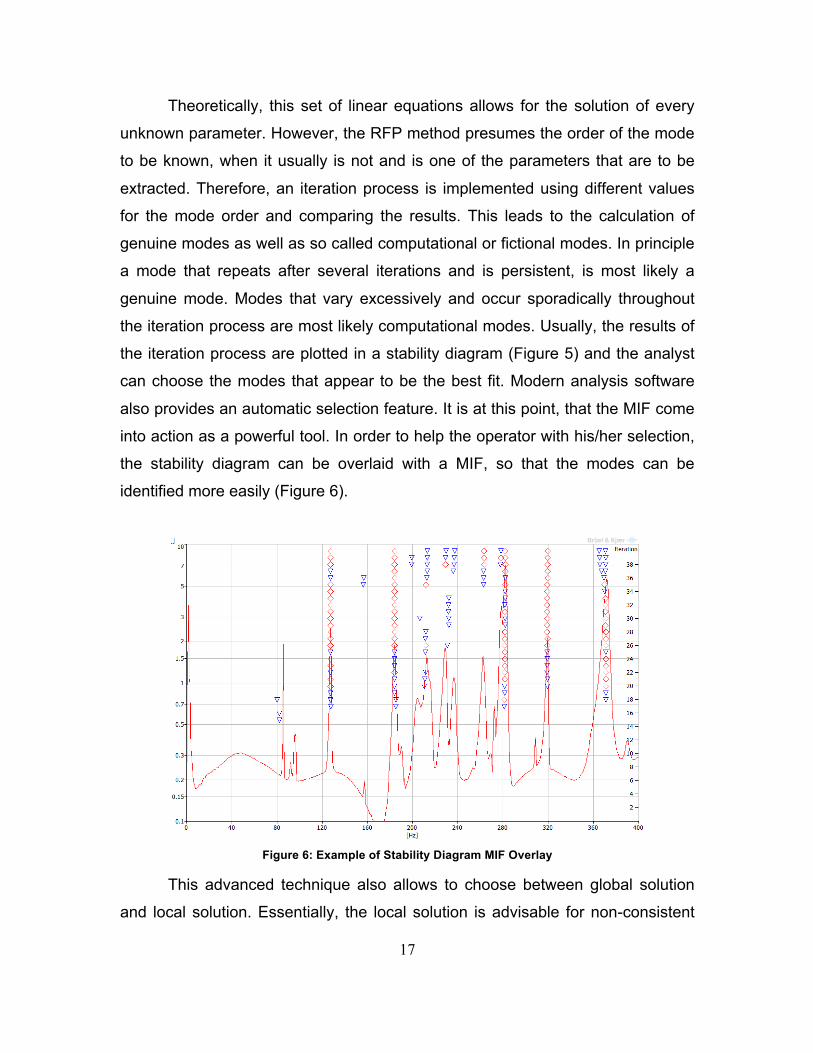
identified more easily (Figure 6).
Figure 6: Example of Stability Diagram MIF Overlay
This advanced technique also allows to choose between global solution
and local solution. Essentially, the local solution is advisable for non-consistent

18
data, which may be caused due to mass-loading. In general, for a complex
structure one may have an inadequate number of accelerometers and is required
to do several measuring cycles during which the accelerometers are moved,
while the force input remains the same Thus, every desired node is measured in
one set of data. However, the change of mass-distribution will cause
discrepancies in the different cycles’ data, resulting in a shift of resonance
frequency. Figure 7 illustrates this effect. Clearly, the resonance appears to be in
a range of frequencies, rather than a single one. The local solution feature allows
for compensation of this effect by calculating a mean value in a specified range.
This mean value is then used for the parameter extraction algorithm.
Figure 7: Example of Frequency Shift
[m/Ns2]
[Hz]

19
C. CORRELATING TEST RESULTS AND SIMULATION RESULTS
In this section, two slightly different concepts shall be discussed. First, the
frequency response assurance criterion (FRAC) is explained, followed by the
introduction of the modal assurance criterion (MAC).
1. Frequency Response Assurance Criterion
The frequency response assurance criterion compares two frequency
response functions and assigns a value between zero and one, with one
representing complete correlation. It is often used for methods with high user
interaction such RFP where the user has to choose a mode on the stability
diagram. In this case, FRAC can be used to correlate the regenerated FRF with
measurement FRF in order to determine whether the parameters extracted
represent a good fit. Ideally, the synthesized and measured FRF should be
linearly related. Furthermore, this feature can be used in any case for validation
of the parameter estimation method. [4] gives the equation this technique uses to
calculate an assurance value:
!"#$!" =!!"(!)!!"∗ (!)
!!!!!!
!
!!"(!)!!"∗ (!)!!!!!! !!"(!)!!"∗ (!)
!!!!!!
(2.25)
2. Modal Assurance Criterion
After the analysis of the experimentally obtained data, the results can be
used to validate a finite element model. For that purpose the modal assurance
criterion has been developed. Although the mode shapes of the simulation and
the shapes of the experiment may differ by number, they can still represent the
same mode, and thus validate the simulation. For further details on MAC, the
reader is referred to [3] and [4].
The modal assurance criterion is a scalar value that can range between
zero and one, with a value close to zero representing low correlation and a value

20
near to one indicating a high correlation. The latter case means that the two
mode shapes represent the same motion but differ by a complex modal scale
factor (MSF). Let m be the total number of modes identified in the bandwidth of
interest, then the MSF is determined by
!"# =!! ! !!!! ! !!
(2.26)
With !!being an m-dimensional vector representing mode shape 1 and !!
being an m-dimensional vector representing mode shape 2. In this notation mode
shape 1 is the reference shape to which shape 2 is compared.
The modal assurance criterion is calculated using the expression
!"# =!!(!) ∗ !!(!)!
!!!!
!!(!) ∗ !!(!)!!!! !!(!) ∗ !!(!)!
!!! (2.27)
There are five reasons why the MAC may take a value near zero:
• the system is non-‐stationary because of changes of mass, stiffness and damping
during testing
• the system is non-‐linear
• there is noise in the reference mode shape
• the chosen parameter extraction technique is invalid
• the mode shapes are linearly independent
If the first four reasons can be eliminated MAC can be used for an
orthogonality check. Although it does not consider mass or stiffness matrices,
MAC can provide an approximation for orthogonality.
The MAC takes a value close to one if:
• the number of DOFs is insufficient to distinguish independent mode shapes
• unmeasured forces to the system influence mode shapes
• the mode shapes consist of coherent noise
21
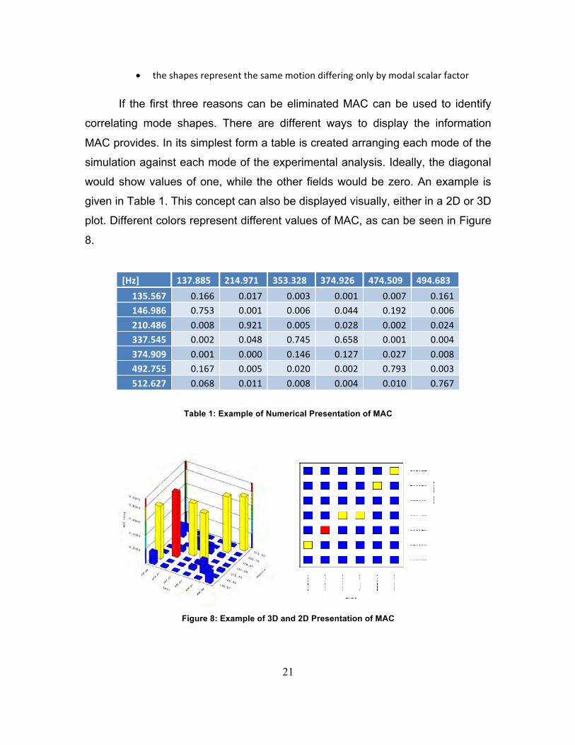
• the shapes represent the same motion differing only by modal scalar factor
If the first three reasons can be eliminated MAC can be used to identify
correlating mode shapes. There are different ways to display the information
MAC provides. In its simplest form a table is created arranging each mode of the
simulation against each mode of the experimental analysis. Ideally, the diagonal
would show values of one, while the other fields would be zero. An example is
given in Table 1. This concept can also be displayed visually, either in a 2D or 3D
plot. Different colors represent different values of MAC, as can be seen in Figure
8.
[Hz] 137.885 214.971 353.328 374.926 474.509 494.683 135.567 0.166 0.017 0.003 0.001 0.007 0.161 146.986 0.753 0.001 0.006 0.044 0.192 0.006 210.486 0.008 0.921 0.005 0.028 0.002 0.024 337.545 0.002 0.048 0.745 0.658 0.001 0.004 374.909 0.001 0.000 0.146 0.127 0.027 0.008 492.755 0.167 0.005 0.020 0.002 0.793 0.003 512.627 0.068 0.011 0.008 0.004 0.010 0.767
Table 1: Example of Numerical Presentation of MAC
Figure 8: Example of 3D and 2D Presentation of MAC

22
THIS PAGE INTENTIONALLY LEFT BLANK
23
III. MODAL TESTING OF NPSAT1
This chapter describes the process of the modal survey of NPSAT1. First
we will examine the test-setup and the reasons for the properties chosen.
Following a brief outline of the test process itself, emphasis will be placed on a
more detailed description of the analysis process.
A. TEST SETUP
The purpose of this thesis is to validate a preliminary run of a finite
element model of NPSAT1. There are some requirements associated with this
task. For further detail on the implications of the choices made in the following
the reader is referred to the preceding Studienarbeit [5].
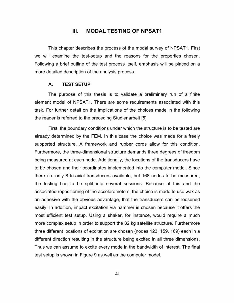
First, the boundary conditions under which the structure is to be tested are
already determined by the FEM. In this case the choice was made for a freely
supported structure. A framework and rubber cords allow for this condition.
Furthermore, the three-dimensional structure demands three degrees of freedom
being measured at each node. Additionally, the locations of the transducers have
to be chosen and their coordinates implemented into the computer model. Since
there are only 8 tri-axial transducers available, but 168 nodes to be measured,
the testing has to be split into several sessions. Because of this and the
associated repositioning of the accelerometers, the choice is made to use wax as
an adhesive with the obvious advantage, that the transducers can be loosened
easily. In addition, impact excitation via hammer is chosen because it offers the
most efficient test setup. Using a shaker, for instance, would require a much
more complex setup in order to support the 82 kg satellite structure. Furthermore
three different locations of excitation are chosen (nodes 123, 159, 169) each in a
different direction resulting in the structure being excited in all three dimensions.
Thus we can assume to excite every mode in the bandwidth of interest. The final
test setup is shown in Figure 9 as well as the computer model.
24
Figure 9: Test Setup Free Boundary Conditions and Computer Model
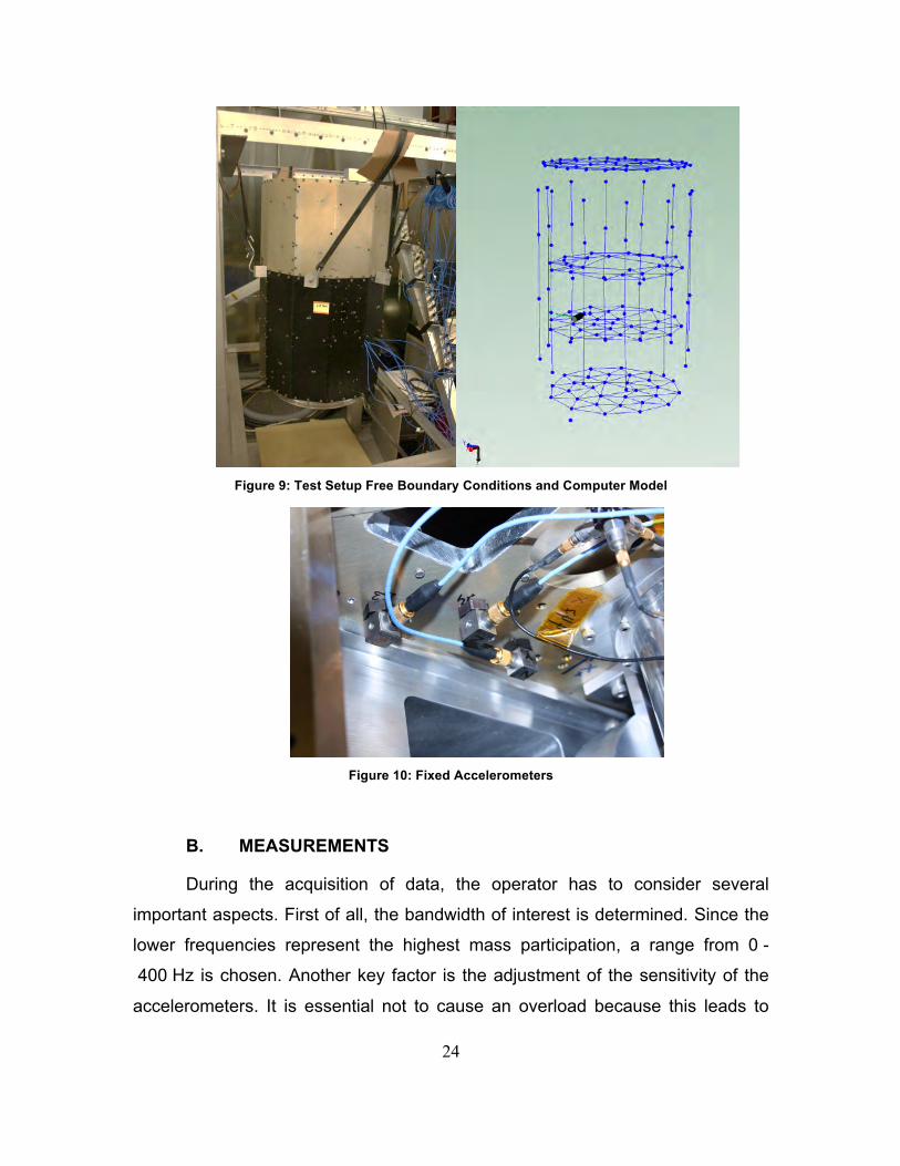
Figure 10: Fixed Accelerometers
B. MEASUREMENTS
During the acquisition of data, the operator has to consider several
important aspects. First of all, the bandwidth of interest is determined. Since the
lower frequencies represent the highest mass participation, a range from 0 -
400 Hz is chosen. Another key factor is the adjustment of the sensitivity of the
accelerometers. It is essential not to cause an overload because this leads to
25
loss of information. However, it is not advisable to have too low a sensitivity
because that introduces noise into the data. Therefore, before starting a
measurement cycle, the sensitivity should be adjusted. In addition, the use of
wax as an adhesive may cause the accelerometers to loosen during data
acquisition. Especially for the measurements taken inside the satellite, this may
not be obvious during the data acquisition. Thus, it is necessary to carefully
check if the accelerometers are still attached after the measurement cycle. It is
advisable to do a preliminary data check after each data acquisition in order to
detect any abnormalities. This possibly saves time during the analysis process if
any cycle has to be repeated or the desired boundary conditions have not been
achieved.
C. MODAL ANALYSIS
During this section we will analyze the obtained data according to the
different methods mentioned in chapter 2. We will follow the path from the easy
and crude SDOF techniques to the more sophisticated MDOF methods. During
the analysis two programs were used. For the SDOF-analysis as well as for the
acquisition of data, the software ‘NX I-deas’ developed by Siemens was used.
For the MDOF-analysis as well as the correlation tasks, ‘PulseReflex’ developed
by Brüel & Kjær was used.
1. Peak-Picking Method on NPSAT1 Data
For initial parameter estimation, we will use the peak-picking method in
order to get an estimate of the modes present. This method represents a fairly
simple technique requiring minimal operator interaction. However, some
limitations may apply because of the rather complex structure.
The first step is to pick the peaks on an FRF graph. During this analysis,
we will emphasize the structural damping and thus use FRF data from the
responses. When viewing the FRF it is already apparent, that the SDOF-
assumption is not fully valid, because of the closely spaced peaks around the 90

26
Hz and 260 Hz area (Figure 11). Furthermore, the range for the analysis is set to
70 Hz – 400 Hz, because of the noise and rigid body modes that appear in the
lower range.
Figure 11: FRF Ref: 123X-; Res: 11X+
After having chosen the frequencies of the peaks, I-deas calculates a
curve-fit. It is also advisable to include residual terms on both ends to
compensate for the influence of out-of-band modes. Comparing the curve-fit
suggestions to the original data, it is obvious that this method does not provide
an accurate estimate for the modal parameters. However, we obtained up to
eleven modes using the Z-direction of excitation and we provide an estimate of
the number of modes to look for using methods that are more sophisticated.
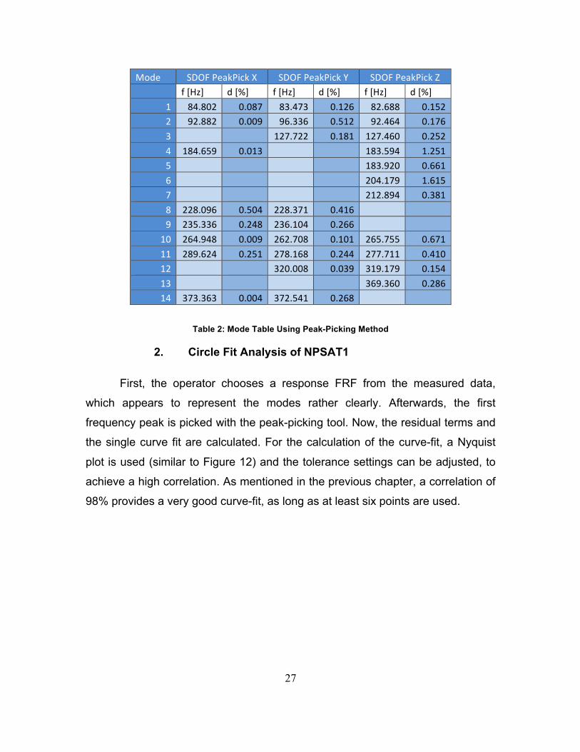
Table 2 shows the results obtained with the peak-pick technique for all three
directions of excitation. Note, that the modes found are already correlated to the
final mode count, thus it can be seen which modes failed to be detected by this
method.
27
Mode SDOF PeakPick X SDOF PeakPick Y SDOF PeakPick Z f [Hz] d [%] f [Hz] d [%] f [Hz] d [%]
1 84.802 0.087 83.473 0.126 82.688 0.152 2 92.882 0.009 96.336 0.512 92.464 0.176 3 127.722 0.181 127.460 0.252 4 184.659 0.013 183.594 1.251 5 183.920 0.661 6 204.179 1.615 7 212.894 0.381 8 228.096 0.504 228.371 0.416 9 235.336 0.248 236.104 0.266
10 264.948 0.009 262.708 0.101 265.755 0.671 11 289.624 0.251 278.168 0.244 277.711 0.410 12 320.008 0.039 319.179 0.154 13 369.360 0.286 14 373.363 0.004 372.541 0.268
Table 2: Mode Table Using Peak-Picking Method
2. Circle Fit Analysis of NPSAT1
First, the operator chooses a response FRF from the measured data,
which appears to represent the modes rather clearly. Afterwards, the first
frequency peak is picked with the peak-picking tool. Now, the residual terms and
the single curve fit are calculated. For the calculation of the curve-fit, a Nyquist
plot is used (similar to Figure 12) and the tolerance settings can be adjusted, to
achieve a high correlation. As mentioned in the previous chapter, a correlation of
98% provides a very good curve-fit, as long as at least six points are used.

28
Figure 12: Circle Fit Nyquist Plot Response 11X+ Reference 123X-
Figure 13: Circle Fit Single Mode Curve Fit
29
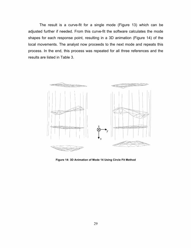
The result is a curve-fit for a single mode (Figure 13) which can be
adjusted further if needed. From this curve-fit the software calculates the mode
shapes for each response point, resulting in a 3D animation (Figure 14) of the
local movements. The analyst now proceeds to the next mode and repeats this
process. In the end, this process was repeated for all three references and the
results are listed in Table 3.
Figure 14: 3D Animation of Mode 14 Using Circle Fit Method
x
z
y

30
Mode CircleFit X CircleFit Y CircleFit Z f [Hz] d [%] f [Hz] d [%] f [Hz] d [%]
1 83.558 0.026 84.527 0.019 86.216 0.246 2 92.970 0.805 94.271 0.689 90.246 0.609 3 122.140 1.020 4 184.712 0.327 185.116 0.187 180.012 1.389 5 204.020 1.470 202.143 1.911 6 213.821 0.522 7 227.786 0.433 229.006 0.116 8 233.787 0.722 233.811 0.900 9 261.742 0.620
10 11 277.457 1.143 12 319.740 0.443 314.065 1.203 13 14 383.873 0.303 373.322 0.057 368.994 1.333
Table 3: Circle-Fit Results
3. Complex Exponential Analysis of NPSAT1 in Frequency Domain
After having gained an overview of possible modes, we can now try to
achieve the best curve-fit and thus the most accurate modal parameters.
Therefore, MDOF techniques represent a more promising approach.
The first step using the complex exponential method is to calculate the
MIF for one set of data. Then, the algorithm can be refined choosing different
options. One very important option is the number of iterations to be used
calculating the stability diagram. In this case, a number of 50 iterations seems
sufficient to distinguish the modes.
As a result, a stability diagram is provided, overlaid with the complex
mode indicator function and one measurement FRF for visual assurance. Figure
15 shows the stability diagram for the Z-reference. The circles represent the

31
modes picked by the operator. The operator chooses the points according to
their influence on the curve-fit and their stabilization. This means that stable
modes are preferred (indicated by a red diamond).
Figure 15: Complex Exponential Mode Selection Z-Reference
Furthermore, the operator constantly watches the FRAC value for the
measurement FRF and regenerated FRF in order to achieve the highest value
possible. Using the complex exponential technique, FRAC values up to 92% can
be achieved. However, FRAC values as low as 20% still exist. The extracted
mode parameters are shown in Table 4.

32
Mode PolyRef Freq X PolyRef Freq Y PolyRef Freq Z f [Hz] d [%] f [Hz] d [%] f [Hz] d [%]
1 85.813 0.058 86.185 0.031 86.917 0.011 2 95.449 0.214 93.983 0.219 93.100 0.061 3 120.919 1.779 127.825 0.302 128.938 0.258 4 184.163 0.595 185.624 0.271 179.375 1.388 5 183.950 0.181 6 203.764 2.317 205.561 3.641 207.777 2.342 7 214.232 0.466 214.887 0.405 213.181 0.937 8 228.200 0.795 229.378 0.870 9 237.687 0.256 235.346 0.954
10 262.839 0.300 262.652 0.502 262.087 0.700 11 276.964 0.417 277.941 0.610 279.128 0.677 12 282.654 0.313 318.550 0.276 13 319.188 0.243 14 372.550 1.002 371.080 0.760 370.635 0.204
Table 4: Modal Parameters Using Complex Exponential Technique
4. Rational Fraction Polynomial Analysis of NPSAT1
In the end, we will use the most sophisticated method available for modal
analysis, the rational fraction polynomial method. First, we will use the global
solution, after which we will move on to the local solution to reduce data
inconsistencies.
The operator’s procedure using the RFP method is very similar to the
complex exponential method. First, the CMIF is calculated and the options of the
algorithm are set. In this case we require 55 iterations to identify the lowest mode
around 85 Hz. Following the settings, the stability diagram is calculated and the
operator can start the curve-fitting process. An example of the stability diagram is
shown in Figure 16. The modes identified using the RFP global method allow for
a FRAC value of up to 95%. Furthermore, the lowest FRAC values are lifted to
around 30%. Thus, we achieved an improvement of accuracy. Table 5 shows the
results of the rational fraction global solution.

33
Figure 16: Stability Diagram RFP Global X-Reference
Mode RFP glob X RFP glob Y RFP glob Z f [Hz] d [%] f [Hz] d [%] f [Hz] d [%]
1 85.482 0.158 85.610 0.085 85.843 0.051 2 94.767 0.001 95.465 0.105 95.113 0.509 3 127.697 0.330 127.372 0.627 127.064 0.424 4 183.894 0.509 184.161 0.750 182.151 0.991 5 190.631 0.137 6 204.541 0.823 202.224 1.494 201.492 0.969 7 213.809 0.832 213.728 0.502 212.551 1.255 8 229.179 0.538 229.337 0.755 231.372 0.841 9 236.096 0.520 236.922 0.525 261.568 0.707
10 263.025 0.478 263.035 0.416 267.525 0.254 11 271.276 0.293 282.032 0.318 280.761 0.285 12 321.021 0.209 319.263 0.217 318.124 0.310 13 368.888 1.458 14 371.472 0.465 370.760 0.768 369.992 0.518
Table 5: Mode Table using RFP Global Solution
However, when scrutinizing the data, it is apparent that frequency shifts
occur during the different measurement cycles. This is most likely caused by

34
mass loading effects. Mass loading occurs when the accelerometers are moved
during the measurement cycles. This results in a slightly different mass
distribution and thus results in a frequency shift of the resonance.
The local solution offers compensation for this effect. Essentially, the
algorithm calculates the modes for each measured FRF and plots it in a cluster
diagram, which is again overlaid with the MIF for visual aid (Figure 17). The
operator can now use an ‘area’-tool to envelop a selection of modes and
calculate the midpoint of that cluster. The extracted parameters are thus a
compromise of all available modes. Furthermore, obvious measurement errors
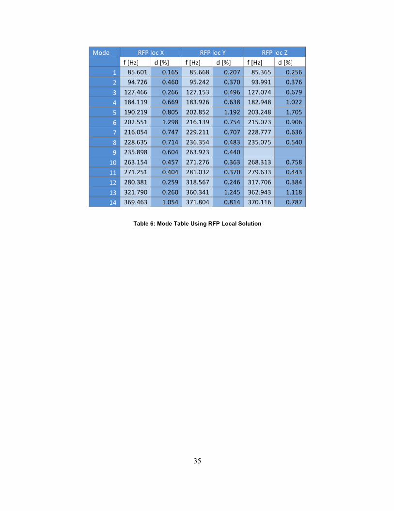
can be left out so they do not influence the result. This method proves to be the
most accurate, as it finds the highest number of modes and allows for a FRAC
value of up to 99%.The average FRAC value is 83.6%. The results are given in
Table 6.
Figure 17: Cluster Diagram RFP Local X-Reference
35
Mode RFP loc X RFP loc Y RFP loc Z f [Hz] d [%] f [Hz] d [%] f [Hz] d [%]
1 85.601 0.165 85.668 0.207 85.365 0.256 2 94.726 0.460 95.242 0.370 93.991 0.376 3 127.466 0.266 127.153 0.496 127.074 0.679 4 184.119 0.669 183.926 0.638 182.948 1.022 5 190.219 0.805 202.852 1.192 203.248 1.705 6 202.551 1.298 216.139 0.754 215.073 0.906 7 216.054 0.747 229.211 0.707 228.777 0.636 8 228.635 0.714 236.354 0.483 235.075 0.540 9 235.898 0.604 263.923 0.440
10 263.154 0.457 271.276 0.363 268.313 0.758 11 271.251 0.404 281.032 0.370 279.633 0.443 12 280.381 0.259 318.567 0.246 317.706 0.384 13 321.790 0.260 360.341 1.245 362.943 1.118 14 369.463 1.054 371.804 0.814 370.116 0.787
Table 6: Mode Table Using RFP Local Solution

36
THIS PAGE INTENTIONALLY LEFT BLANK
37
IV. CONCLUSION AND OUTLOOK
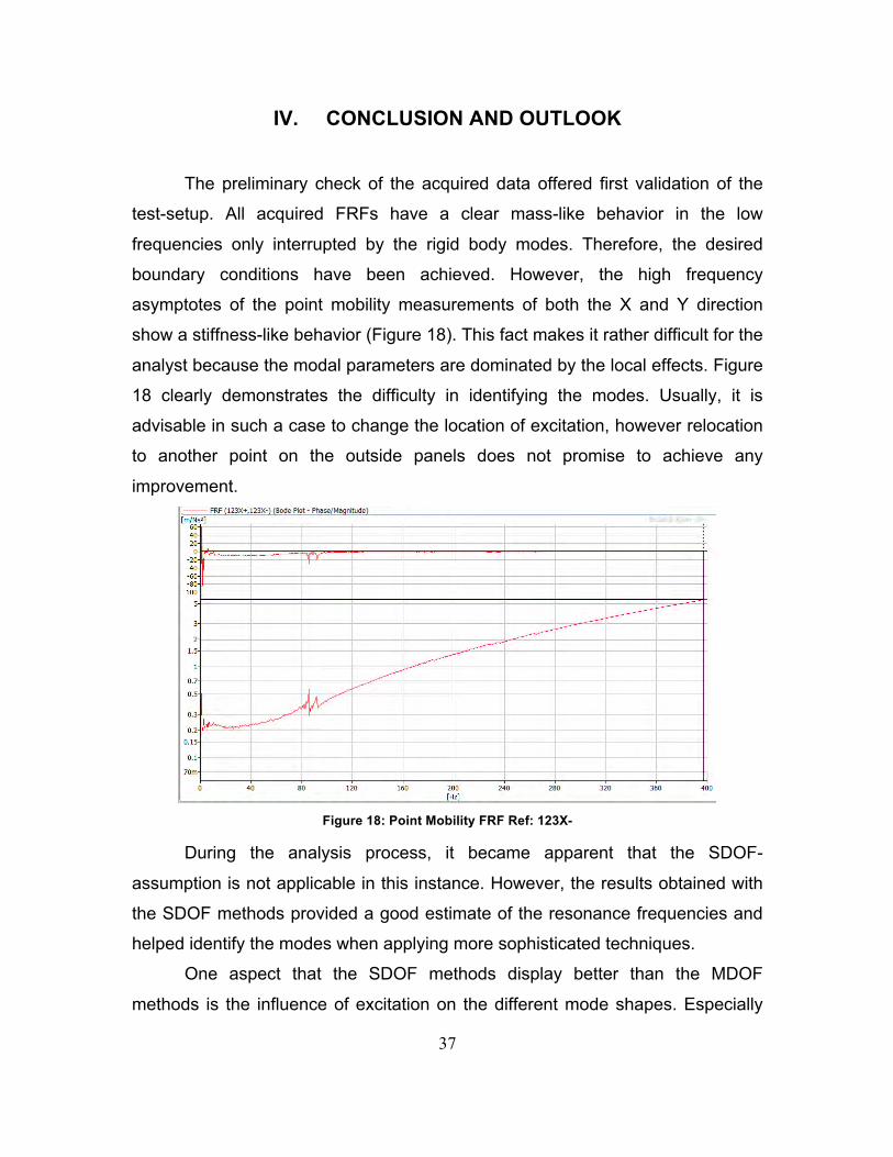
The preliminary check of the acquired data offered first validation of the
test-setup. All acquired FRFs have a clear mass-like behavior in the low
frequencies only interrupted by the rigid body modes. Therefore, the desired
boundary conditions have been achieved. However, the high frequency
asymptotes of the point mobility measurements of both the X and Y direction
show a stiffness-like behavior (Figure 18). This fact makes it rather difficult for the
analyst because the modal parameters are dominated by the local effects. Figure
18 clearly demonstrates the difficulty in identifying the modes. Usually, it is
advisable in such a case to change the location of excitation, however relocation
to another point on the outside panels does not promise to achieve any
improvement.
Figure 18: Point Mobility FRF Ref: 123X-
During the analysis process, it became apparent that the SDOF-
assumption is not applicable in this instance. However, the results obtained with
the SDOF methods provided a good estimate of the resonance frequencies and
helped identify the modes when applying more sophisticated techniques.
One aspect that the SDOF methods display better than the MDOF
methods is the influence of excitation on the different mode shapes. Especially

38
the circle fit method showed that certain mode shapes are excited better in one
direction than the other.
Since the RFP local solution in X direction offers the best curve-fit, it is
chosen to correlate to the FEM results in order to validate the model. For this
task a MAC graph is calculated (Figure 19). As can be seen in the graph the
mode shapes correlate very badly. Moreover, the first mode calculated by the
FEM simulation is located at 200.674 Hz which is significantly higher than the
first mode identified by modal testing (85.601 Hz; RFP local X).
Figure 19: MAC Simulation vs. RFP local X-Reference
Figure 20: 3D MAC Simulation vs. RFP local X-Reference
Simulation
RFP
loca
l X-R
efer
ence

39
Therefore, the FEM is considerably stiffer than the actual structure. This
results from the connections in the model which represent a welded connection
rather than a connection by screws. As a result, the FEM has to be modified by
considering the connection conditions of each part. The model has to be more
flexible for it to reproduce the actual structure of NPSAT1.
In order to validate the test results, each mode table is correlated to the
RFP local X-Reference table. Thus, we can determine if the acquired results are
consistent. First, it is obvious that even the SDOF-methods identify modes that
are in the same range as the modes found by the other techniques. Furthermore,
when correlating the results of the MDOF techniques with the RFP local X
Reference, a clear diagonal trend is apparent. Thus, we can assume that the test
results are in fact valid.
In conclusion, the test results appear to be genuine and the test-setup
provides the demanded boundary conditions. The correlation with the finite
element model, however, proves to be poor and thus the model has to be
improved. It is suggested that the model is made more flexible in order to
reproduce the effects found during the testing. When the FEM has been adapted,
it can be correlated again with the test results and no additional modal analysis is
necessary.

40
THIS PAGE INTENTIONALLY LEFT BLANK

41
V. LIST OF REFERENCES
[1] D. Sakoda, J. A. Horning and S. D. Moseley, Naval Postgraduate School NPSAT1 Small Satellite, 2006.
[2] D. J. Ewins, Modal Testing: Theory, Practice and Application, Second ed., Hertfordshire: Research Studies Press Ltd., 2000.
[3] Siemens, NX I-deas Help Files. [4] R. J. Allemang, "The Modal Assurance Criterion - Twenty Years of Use and
Abuse," Sound and Vibration, August 2003. [5] S. Rahn, "Modal Test of a Substructure of NPSAT1," Monterey, 2012. [6] Agilent Technologies, The Fundamentals of Modal Testing, 1997. [7] D. J. Ewins, Modal Testing: Theory and Practice, Somerset: Research Studies
Press Ltd., 1984. [8] J. P. D. Hartog, Mechanical Vibrations, McGraw-Hill Book Company Inc.,
1956. [9] Brüel & Kjaer, PulseReflex Help Files.


