Download - MULTIDIMENSIONAL SCALING: AN INTRODUCTION
MULTIDIMENSIONAL SCALING:AN INTRODUCTION
William G. JacobyMichigan State University and ICPSR
Workshop in MethodsIndiana UniversityDecember 7, 2012
E-mail: [email protected]: http://polisci.msu.edu/jacoby/iu/mds2012
Begin with an Example
Assume we have information about the Americanelectorate’s perceptions of thirteen prominent politicalfigures from the period of the 2004 presidential election.
Specifically, we have the perceived dissimilarities betweenall pairs of political figures.
With 13 figures, there will be 78 distinct pairs of figures.
Rank-order pairs of political figures, according to theirdissimilarity (from least to most dissimilar).
For convenience, arrange the rank-ordered dissimilarityvalues into a square, symmetric matrix.

Matrix of Perceptual Dissimilarities among 2004Political Figures
George W Bush 0.0 73.0 62 8.0 68.0 20.0 51.5 41.0 24.0 7 25.5 50 5.0John Kerry 73.0 0.0 56 78.0 1.0 54.0 15.0 17.0 47.0 77 37.0 2 74.5Ralph Nader 62.0 56.0 0 72.0 59.0 53.0 60.0 49.0 58.0 70 39.0 57 71.0Dick Cheney 8.0 78.0 72 0.0 74.5 25.5 65.0 51.5 29.0 12 30.0 66 4.0John Edwards 68.0 1.0 59 74.5 0.0 44.0 14.0 16.0 46.0 76 38.0 3 69.0Laura Bush 20.0 54.0 53 25.5 44.0 0.0 42.0 34.0 9.5 23 22.0 45 18.0Hillary Clinton 51.5 15.0 60 65.0 14.0 42.0 0.0 19.0 32.0 67 40.0 13 55.0Bill Clinton 41.0 17.0 49 51.5 16.0 34.0 19.0 0.0 31.0 61 36.0 11 48.0Colin Powell 24.0 47.0 58 29.0 46.0 9.5 32.0 31.0 0.0 28 9.5 35 21.0John Ashcroft 7.0 77.0 70 12.0 76.0 23.0 67.0 61.0 28.0 0 33.0 63 6.0John McCain 25.5 37.0 39 30.0 38.0 22.0 40.0 36.0 9.5 33 0.0 43 27.0Democratic Pty 50.0 2.0 57 66.0 3.0 45.0 13.0 11.0 35.0 63 43.0 0 64.0Republican Pty 5.0 74.5 71 4.0 69.0 18.0 55.0 48.0 21.0 6 27.0 64 0.0
Clearly, there is too much information in this matrix to becomprehensible in its “raw” numeric form!
Instead, try “drawing a picture” of the information in thematrix.

Rules for Drawing the Picture
Each political figure is shown as a point.
Points are located on the surface of the display medium.
For example, the projection screen or a sheet of paper
In any case, a two-dimensional space
Adjust the point locations so that the rank-order of thedistances between pairs of points corresponds as closelyas possible to the rank-ordered dissimilarities betweenpairs of political figures.
The process of constructing the picture from thedissimilarities is multidimensional scaling.

MDS Point Configuration of 2004 Political Figures
MDS Axis 1
MD
S A
xis
2
0
1
2
-1 0 1
G BushKerry
Nader
CheneyEdwards
L Bush
H Clinton
B Clinton Powell
Ashcroft
McCain
Dem Pty Rep Pty

A General Definition of Multidimensional Scaling
A family of procedures for constructing a spatial model ofobjects, using information about the proximities betweenthe objects.
Different “varieties” of MDS
Classical multidimensional scaling (CMDS)
Weighted multidimensional scaling (WMDS)
Unfolding models (or “ideal points models”)
Preference mapping (or “the vector model of preferences”)
Correspondence analysis (CA)

Utility of MDS for Social Research
Reducing dimensionality
Modeling perceptions of survey respondents orexperimental subjects
Flexible with respect to input data
Useful measurement tool
Graphical output
The Map Analogy
A Familiar Task:
Starting with a map (a geometric model)
Can obtain the distances between locations (numeric data)
MDS “Reverses” the Preceding Task:
We begin with distances (numeric data)
Use that information to produce a map (geometric model)

More Formal Representation
Begin with a k × k symmetric matrix, ∆, of “proximities”among k objects.
The proximity between the object represented by the i th rowand the object represented by the j th column is shown bythe cell entry, δij .
Greater proximity between objects i and j corresponds tosmaller values of δij and vice versa.
Therefore, the proximities are often called “dissimilarities.”
Admittedly, this terminology is a bit confusing!
But, there is a reason for it . . .
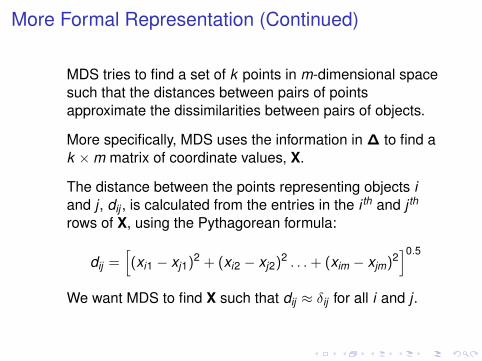
More Formal Representation (Continued)
MDS tries to find a set of k points in m-dimensional spacesuch that the distances between pairs of pointsapproximate the dissimilarities between pairs of objects.
More specifically, MDS uses the information in ∆ to find ak ×m matrix of coordinate values, X.
The distance between the points representing objects iand j , dij , is calculated from the entries in the i th and j th
rows of X, using the Pythagorean formula:
dij =[(xi1 − xj1)2 + (xi2 − xj2)2 . . .+ (xim − xjm)2
]0.5
We want MDS to find X such that dij ≈ δij for all i and j .
More Formal Representation (Continued)
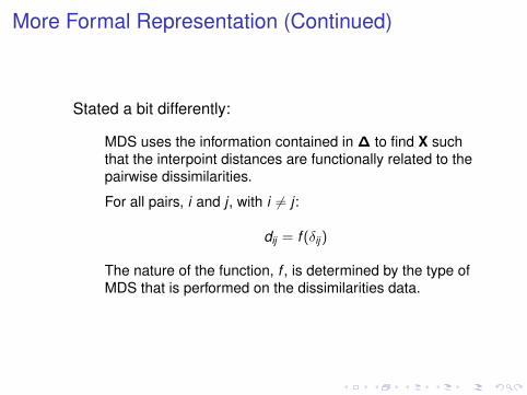
Stated a bit differently:
MDS uses the information contained in ∆ to find X suchthat the interpoint distances are functionally related to thepairwise dissimilarities.
For all pairs, i and j , with i 6= j :
dij = f (δij )
The nature of the function, f , is determined by the type ofMDS that is performed on the dissimilarities data.

Metric MDS
Metric multidimensional scaling requires that distances arerelated to dissimilarities by a linear function:
dij = a + b δij + eij
In the preceding formula, a and b are coefficients to beestimated, and eij is an error term associated with objects iand j .
Stated differently, metric MDS assumes that the inputdissimilarities data are measured at the interval or ratiolevel.

Torgerson’s Procedure for Metric MDS, I
Begin with k × k dissimilarities matrix, ∆
Assume the dissimilarities correspond to distances inm-dimensional space (except for random error)
The k × k matrix of distances between points is D.
The k × k matrix, E, contains random errors.
Hypothesis:∆ = D + E
Objective (stated informally):Find the k ×m coordinate matrix, X, such that entries in Eare as close to zero as possible.
Torgeron’s Procedure for Metric MDS, II
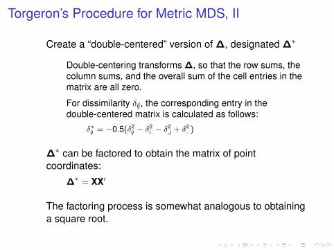
Create a “double-centered” version of ∆, designated ∆∗
Double-centering transforms ∆, so that the row sums, thecolumn sums, and the overall sum of the cell entries in thematrix are all zero.
For dissimilarity δij , the corresponding entry in thedouble-centered matrix is calculated as follows:
δ∗ij = −0.5(δ2ij − δ2
i. − δ2.j + δ2
..)
∆∗ can be factored to obtain the matrix of pointcoordinates:
∆∗ = XX′
The factoring process is somewhat analogous to obtaininga square root.
Torgeron’s Procedure for Metric MDS, III
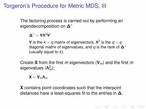
The factoring process is carried out by performing aneigendecomposition on ∆∗
∆∗ = VΛ2V′
V is the k × q matrix of eigenvectors, Λ2 is the q × qdiagonal matrix of eigenvalues, and q is the rank of ∆∗
(usually equal to k ).
Create X from the first m eigenvectors (Vm) and the first meigenvalues (Λ2
m):
X = VmΛm
X contains point coordinates such that the interpointdistances have a least-squares fit to the entries in ∆.

Example, Using Ten American Cities
Driving distances between ten cities (in thousands of miles):Table 1: Table of driving distances between ten American cities (in thousands of miles).
0 0.587 1.212 0.701 1.936 0.604 0.748 2.139 2.182 0.543 ATLANTA 0.587 0 0.920 0.940 1.745 1.188 0.713 1.858 1.737 0.597 CHICAGO 1.212 0.920 0 0.879 0.831 1.726 1.631 0.949 1.021 1.494 DENVER 0.701 0.940 0.879 0 1.374 0.968 1.420 1.645 1.891 1.220 HOUSTON 1.936 1.745 0.831 1.374 0 2.339 2.451 0.347 0.959 2.300 LOS ANGELES 0.604 1.188 1.726 0.968 2.339 0 1.092 2.594 2.734 0.923 MIAMI 0.748 0.713 1.631 1.420 2.451 1.092 0 2.571 2.408 0.205 NEW YORK 2.139 1.858 0.949 1.645 0.347 2.594 2.571 0 0.678 2.442 SAN FRANCISCO 2.182 1.737 1.021 1.891 0.959 2.734 2.408 0.678 0 2.329 SEATTLE 0.543 0.597 1.494 1.229 2.300 0.923 0.205 2.442 2.329 0 WASHINGTON DC
The preceding ∆ is a good example for metric MDS:
We already know m (the dimensionality)
We already know the “shape” of the point configuration

Double-centered version of intercity distance matrix
The following matrix is the ∆∗ obtained whenTorgerson’s transformation is applied to all cells
of the intercity distance matrix, ∆.Table 2: Double-centered version of intercity driving distance matrix.
0.537 0.228 -0.348 0.199 -0.808 0.895 0.697 -1.005 -1.050 0.656 0.228 0.263 -0.174 -0.134 -0.594 0.234 0.585 -0.581 -0.315 0.488 -0.348 -0.174 0.236 -0.092 0.570 -0.563 -0.504 0.681 0.658 -0.463 0.199 -0.134 -0.092 0.352 0.029 0.516 -0.124 -0.163 -0.550 -0.033 -0.808 -0.594 0.570 0.029 1.594 -1.130 -1.499 1.751 1.399 -1.313 0.895 0.234 -0.563 0.516 -1.130 1.617 0.920 -1.542 -1.867 0.918 0.697 0.585 -0.504 -0.124 -1.499 0.920 1.416 -1.583 -1.130 1.222 -1.005 -0.581 0.681 -0.163 1.751 -1.542 -1.583 2.028 1.846 -1.432 -1.050 -0.315 0.658 -0.550 1.399 -1.867 -1.130 1.846 2.124 -1.115 0.656 0.488 -0.463 -0.033 -1.313 0.918 1.222 -1.432 -1.115 1.071
An eigendecomposition is carried out on the preceding ∆∗.
We expect a two-dimensional solution, so we use the firsttwo eigenvectors and the first two eigenvalues.
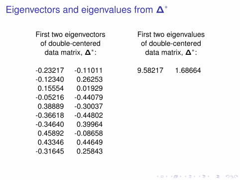
Eigenvectors and eigenvalues from ∆∗
First two eigenvectors First two eigenvaluesof double-centered of double-centered
data matrix, ∆∗: data matrix, ∆∗:
-0.23217 -0.11011 9.58217 1.68664-0.12340 0.262530.15554 0.01929
-0.05216 -0.440790.38889 -0.30037
-0.36618 -0.44802-0.34640 0.399640.45892 -0.086580.43346 0.44649
-0.31645 0.25843

Rescaled Eigenvectors
The eigenvectors are multiplied by the square roots ofthe corresponding eigenvalues to produce the matrix oftwo-dimensional point coordinates: X = V2Λ2
-0.71867 -0.14300 Atlanta-0.38197 0.34095 Chicago0.48149 0.02505 Denver
-0.16147 -0.57246 Houston1.20382 -0.39009 Los Angeles
-1.13352 -0.58185 Miami-1.07228 0.51901 New York1.42058 -0.11244 San Francisco1.34179 0.57986 Seattle
-0.97958 0.33562 Washington D.C.
Point coordinates can be plotted in two-dimensional space

Point Configuration from Metric MDS
Graph of the rescaled eigenvectors:
First rescaled eigenvector
Sec
ond
resc
aled
eig
enve
ctor
−1
0
1
−1 0 1
●
●
●
●
●
●
●
●
●
●
Atlanta
Chicago
Denver
Houston
Los Angeles
Miami
New York
San Francisco
Seattle
Washington DC

Revised Point Configuration from Metric MDS
Graph of the rescaled eigenvectors, first eigenvector reflected:
First rescaled eigenvector, reflected
Sec
ond
resc
aled
eig
enve
ctor
−1
0
1
−1 0 1
●
●
●
●
●
●
●
●
●
●
Atlanta
Chicago
Denver
Houston
Los Angeles
Miami
New York
San Francisco
Seattle
Washington DC
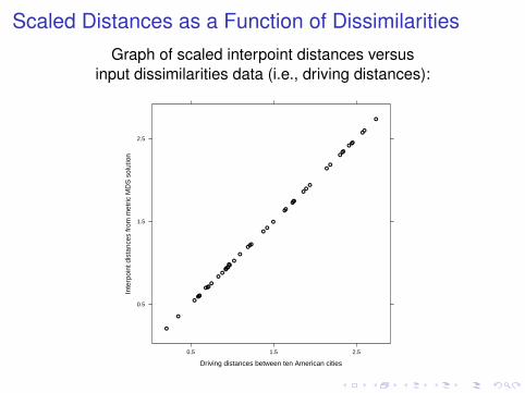
Scaled Distances as a Function of DissimilaritiesGraph of scaled interpoint distances versus
input dissimilarities data (i.e., driving distances):
Driving distances between ten American cities
Inte
rpoi
nt d
ista
nces
from
met
ric M
DS
sol
utio
n
0.5
1.5
2.5
0.5 1.5 2.5
●
●
●
●
●
●
●●
●
●●
●
●
●
●
●
●
●●
●
●
●
●
●
●
●
●
●
●
●
●
●
●
●
●
●
●
●
●
●
●
●
●
●
●

Model Fit, Graphical Assessment
Eigenvalues are related to the variance in thedouble-centered distances that is “explained” by eacheigenvector.
The “Scree plot” shows the eigenvalues plotted in the orderthat they were factored from the dissimilarities matrix.
Useful visual representation of model fit
Logic:
The “important” dimensions in a metric MDS solutionshould account for a large part of the variance in thedissimilarities data.
Dimensions associated primarily with error should accountfor very little variance.

Scree Plot for Metric MDS SolutionGraph of eigenvalues versus order of extraction
in metric MDS of intercity driving distances:
Eigenvector
Eig
enva
lue
0
2
4
6
8
10
2 4 6 8 10
Goodness of Fit Measure for Metric MDS
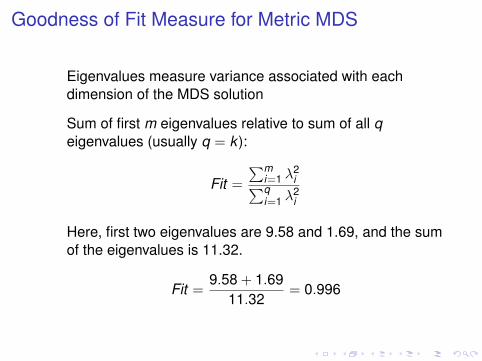
Eigenvalues measure variance associated with eachdimension of the MDS solution
Sum of first m eigenvalues relative to sum of all qeigenvalues (usually q = k ):
Fit =
∑mi=1 λ
2i∑q
i=1 λ2i
Here, first two eigenvalues are 9.58 and 1.69, and the sumof the eigenvalues is 11.32.
Fit =9.58 + 1.69
11.32= 0.996

A Conceptual Leap
So far, we have used physical distances as the input data.
If MDS works for physical distances, then it may also workfor data that can be interpreted as “conceptual distances.”
Many types of data can be interpreted as conceptualdistances.
Usually correspond to ideas like “proximity” and similarity(or dissimilarity)
We will say more about this later . . .
Profile Dissimilarities
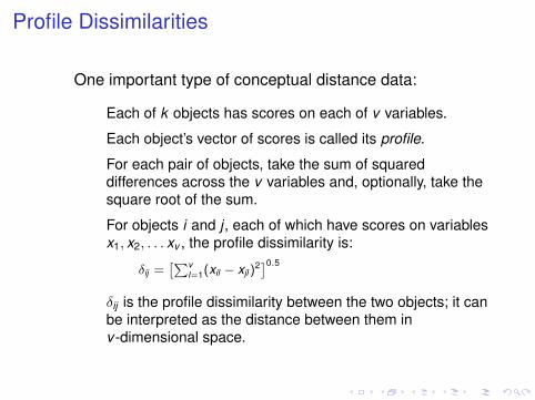
One important type of conceptual distance data:
Each of k objects has scores on each of v variables.
Each object’s vector of scores is called its profile.
For each pair of objects, take the sum of squareddifferences across the v variables and, optionally, take thesquare root of the sum.
For objects i and j , each of which have scores on variablesx1, x2, . . . xv , the profile dissimilarity is:
δij =[∑v
l=1(xil − xjl)2]0.5
δij is the profile dissimilarity between the two objects; it canbe interpreted as the distance between them inv -dimensional space.

Substantive Example, Using Same Ten Cities
Socioeconomic characteristics of ten American cities:Table 3: Socioeconomic characteristics of ten American cities.
Climate,Terrain Housing
Environ.,Health Crime
Transport-ation Education The Arts Recreation Economics
AtlantaChicagoDenver
HoustonLA
MiamiNYCSF
SeattleDC
0.185-0.942-0.899-1.500 1.356-0.198-0.174 1.511 0.879-0.217
-1.338-0.350-0.397-0.789 0.774-0.596 0.580 2.026-0.628 0.719
-0.451 0.977-0.820-0.856 0.636-0.941 2.135-0.156-0.718 0.196
-0.609-1.139-0.498-0.239 0.652 1.617 1.692-0.007-0.876-0.591
0.817 0.423 0.661-1.419-1.585-1.078 0.945 0.752-0.231 0.715
-0.413 1.112-0.100 0.347 0.077-1.046-0.673 0.703-1.647 1.642
-0.700 0.431-0.640-0.470 0.347-0.879 2.520-0.264-0.568 0.225
-1.352-0.201-0.611-0.995 0.640 0.911 0.355 1.142 1.297-1.186
0.327-1.142 1.451 1.848-0.995-0.301-0.966-0.006-0.220 0.005
Table entries are standardized versions of scores assigned to cities in Places Rated Almanac, by RichardBoyer and David Savageau The data are used here with the kind permission of the publisher, Rand McNally.For all but two of the above criteria, the higher the score, the better. For Housing and Crime, the lower thescore the better.
Table entries are standardized versions of scores assigned to cities in PlacesRated Almanac, by Richard Boyer and David Savageau. The data are used herewith the kind permission of the publisher, Rand McNally. For all but two of theabove criteria, the higher the score, the better. For Housing and Crime, the lowerthe score the better.
Use this information to calculate the 10× 10 matrix, ∆, of profile dissimilaritiesbetween the cities.

Profile Dissimilarities Matrix
Profile dissimilarities matrix, ∆∗:Table 4: Matrix of profile dissimilarities for ten American cities.
Atlanta 0.000 3.438 2.036 3.394 4.630 3.930 5.555 4.615 3.330 3.168 Chicago 3.438 0.000 3.635 4.364 3.964 4.740 4.357 4.253 4.299 2.296 Denver 2.036 3.635 0.000 2.333 4.849 3.794 5.674 4.285 3.606 2.994 Houston 3.394 4.364 2.333 0.000 5.016 3.959 6.453 5.517 4.588 3.911 Los Angeles 4.630 3.964 4.849 5.016 0.000 3.361 4.181 3.180 3.611 4.039 Miami 3.930 4.740 3.794 3.959 3.361 0.000 5.234 4.471 2.959 4.906 New York 5.555 4.357 5.674 6.453 4.181 5.234 0.000 4.930 5.535 4.796San Francisco 4.615 4.253 4.285 5.517 3.180 4.471 4.930 0.000 3.894 3.422 Seattle 3.330 4.299 3.606 4.588 3.611 2.959 5.535 3.894 0.000 4.744Washington DC 3.168 2.296 2.994 3.911 4.039 4.906 4.796 3.422 4.744 0.000
Matrix entries are obtained by taking the sum of squared differences between all pairs of rows in Table 3.Apply Torgerson’s formula to double-center this matrix.

Double-Centered Profile Dissimilarities
The ∆∗ matrix:
Atlanta 5.668 0.028 3.373 2.289 -4.232 -0.963 -4.318 -3.394 0.925 0.623 Chicago 0.028 6.211 -0.889 -1.201 -1.097 -4.205 1.890 -1.515 -2.498 3.277 Denver 3.373 -0.889 5.226 5.104 -5.490 -0.658 -5.212 -2.143 -0.251 0.940 Houston 2.289 -1.201 5.104 10.430 -3.712 1.303 -7.334 -5.579 -1.674 0.374 Los Angeles -4.232 -1.097 -5.490 -3.712 7.310 1.931 3.191 3.021 0.771 -1.693 Miami -0.963 -4.205 -0.658 1.303 1.931 7.851 -1.499 -1.644 3.183 -5.298 New York -4.318 1.890 -5.212 -7.334 3.191 -1.499 16.554 0.548 -3.404 -0.416San Francisco -3.394 -1.515 -2.143 -5.579 3.021 -1.644 0.548 8.849 0.477 1.379 Seattle 0.925 -2.498 -0.251 -1.674 0.771 3.183 -3.404 0.477 7.275 -4.805Washington DC 0.623 3.277 0.940 0.374 -1.693 -5.298 -0.416 1.379 -4.805 5.619
Use eigendecomposition to obtain metric MDS solution
But, an important preliminary question . . .

Assessing Dimensionality
What is appropriate dimensionality for the metric MDSsolution?
Could be any number up to k − 1
Competing considerations:
Enough dimensions to account for sufficient variance
Relatively few dimensions to facilitate interpretation
Try examining the scree plot.

Evidence from Scree Plot
Scree plot for eigendecomposition of ∆∗ matrix:
Eigenvector
Eig
enva
lue
0
5
10
15
20
25
30
2 4 6 8 10

Interpreting Scree Plot Evidence
No obvious “elbow” in scree plot
No clear distinction between “important” and “unimportant”dimensions, in terms of variance explained.
Use parsimony for guidance
Use m = 2 so we can visualize the MDS solution easily.

Metric MDS SolutionTwo-dimensional point configuration obtained from metric MDS
of double- centered matrix of profile dissimilarities.
First rescaled eigenvector
Sec
ond
resc
aled
eig
enve
ctor
−2
0
2
−2 0 2
●
●
●
●
●
●
●
●
●
●
Chicago
Denver
Houston
Los Angeles
Miami
New York
San Francisco
Seattle
Washington DC
Atlanta

Goodness of Fit
Calculate fit statistic for the metric MDS solution:
Fit =
∑mi=1 λ
2i∑q
i=1 λ2i
=30.337 + 20.046
81= 0.622
The two-dimensional MDS solution “explains” about 60percent of the variance in the profile dissimilarities
Remaining variance is error
We have assumed the error is random
Is it?

Assessing Errors in Metric MDS Solution
Shepard Diagram for Metric MDS of City Characteristics:
Profile dissimilarities
Inte
rpoi
nt d
ista
nces
in 2
−D
MD
S c
onfig
urat
ion
1
3
5
2 4 6
●
●
●
●
●
●
●
●
●
●
●
●
●
●
●
●
●
●
●
●
●
●
●
●
●
●
●
●
●●
●
●
●
●
●
●
●
●
●
●
●
●
●
●
●

Assessing Errors in Metric MDS Solution
Shepard Diagram for Metric MDS of City Characteristics:
Profile dissimilarities
Inte
rpoi
nt d
ista
nces
in 2
−D
MD
S c
onfig
urat
ion
1
3
5
2 4 6
●
●
●
●
●
●
●
●
●
●
●
●
●
●
●
●
●
●
●
●
●
●
●
●
●
●
●
●
●●
●
●
●
●
●
●
●
●
●
●
●
●
●
●
●

Assessing Errors in Metric MDS Solution
Shepard Diagram for Metric MDS of City Characteristics:
Profile dissimilarities
Inte
rpoi
nt d
ista
nces
in 2
−D
MD
S c
onfig
urat
ion
1
3
5
2 4 6
●
●
●
●
●
●
●
●
●
●
●
●
●
●
●
●
●
●
●
●
●
●
●
●
●
●
●
●
●●
●
●
●
●
●
●
●
●
●
●
●
●
●
●
●

A New Concern
Distances in MDS solution do not appear to be a linearfunction of the dissimilarities.
Instead, distances seem to be monotonically related todissimilarities.
Distances are monotonically related to dissimilarities if, forall i , j , and l , the following holds:
δij < δil =⇒ dij ≤ dil
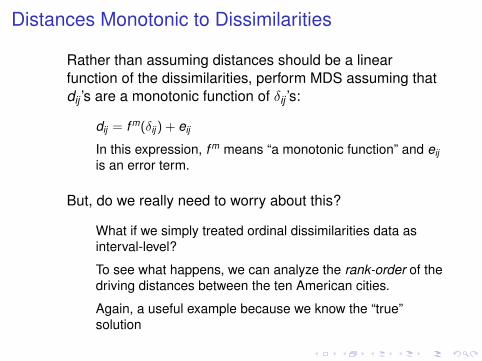
Distances Monotonic to Dissimilarities
Rather than assuming distances should be a linearfunction of the dissimilarities, perform MDS assuming thatdij ’s are a monotonic function of δij ’s:
dij = f m(δij ) + eij
In this expression, f m means “a monotonic function” and eijis an error term.
But, do we really need to worry about this?
What if we simply treated ordinal dissimilarities data asinterval-level?
To see what happens, we can analyze the rank-order of thedriving distances between the ten American cities.
Again, a useful example because we know the “true”solution
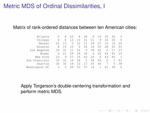
Metric MDS of Ordinal Dissimilarities, I
Matrix of rank-ordered distances between ten American cities:
Atlanta 0 4 22 8 34 6 10 35 36 3 Chicago 4 0 13 15 31 21 9 32 30 5 Denver 22 13 0 12 11 29 27 16 19 26 Houston 8 15 12 0 24 18 25 28 33 23 Los Angeles 34 31 11 24 0 39 42 2 17 37 Miami 6 21 29 18 39 0 20 44 45 14 New York 10 9 27 25 42 20 0 43 40 1 San Francisco 35 32 16 28 2 44 43 0 7 41 Seattle 36 30 19 33 17 45 40 7 0 38 Washington DC 3 5 26 23 37 14 1 41 38 0
Apply Torgerson’s double-centering transformation andperform metric MDS.
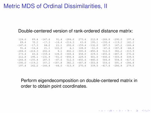
Metric MDS of Ordinal Dissimilarities, II
Double-centered version of rank-ordered distance matrix:Table 6: Double-centered version of rank-ordered intercity distance matrix.
124.6 89.4 -147.6 91.4 -284.6 273.4 212.8 -266.8 -290.0 197.4 89.4 70.2 -17.3 -16.4 -214.3 43.6 195.1 -193.4 -119.2 162.2-147.6 -17.3 64.2 21.1 202.6 -159.4 -132.0 187.5 147.2 -166.4 91.4 -16.4 21.1 122.0 4.1 128.0 -51.0 -47.6 -187.8 -64.0-284.6 -214.3 202.6 4.1 462.2 -300.4 -450.4 512.5 382.2 -313.9 273.4 43.6 -159.4 128.0 -300.4 458.0 229.5 -455.6 -487.8 270.6 212.8 195.1 -131.9 -51.0 -450.4 229.5 401.0 -440.6 -303.8 339.5-266.8 -193.4 187.5 -47.6 512.5 -455.6 -440.6 566.8 554.6 -417.6-290.0 -119.2 147.2 -187.8 382.2 -487.8 -303.8 554.6 591.4 -286.8 197.4 162.2 -166.4 -64.0 -313.9 270.6 339.5 -417.6 -286.8 279.0
Perform eigendecomposition on double-centered matrix inorder to obtain point coordinates.

Metric MDS of Ordinal Dissimilarities, III
The point coordinate matrix, X = V2Λ2, obtained fromeigendecomposition of the double-centered, rank-ordered,
distance matrix:
Rescaled Eigenvectors:The following are the point coordinates obtained
by performing a metric MDS (i.e., eigendecompositionof the double-centered matrix) on rank-ordered distances.
Dim 1 Dim 2Atlanta 12.699841 -2.0733232Chicago 7.518241 5.8125445Denver -8.266138 -1.2161737Houston 2.508042 -10.8456988LA -20.611218 -6.5285933Miami 18.556184 -9.7896715NYC 17.935017 9.4370549SF -24.342714 -0.5662753Seattle -21.999173 10.2237850DC 16.001918 5.5463514

Metric MDS of Ordinal Dissimilarities, IV
Two-dimensional configuration obtained from metric MDS ofrank-ordered intercity distances:
First rescaled eigenvector, reflected
Sec
ond
resc
aled
eig
enve
ctor
, ref
lect
ed
−20
0
20
−20 0 20
●
●
●
●
●
●
●
●
●
●
AtlantaDenver
Houston
Los Angeles
Miami
New York
San Francisco
Seattle
Washington DCChicago
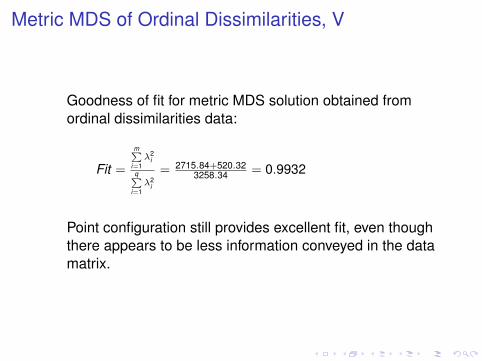
Metric MDS of Ordinal Dissimilarities, V
Goodness of fit for metric MDS solution obtained fromordinal dissimilarities data:
Fit =
m∑i=1λ2
i
q∑i=1λ2
i
= 2715.84+520.323258.34 = 0.9932
Point configuration still provides excellent fit, even thoughthere appears to be less information conveyed in the datamatrix.

Assessment
Metric MDS of ordinal data seems to work . . .
But, it is problematic
It is “cheating” with respect to data characteristics.
It imposes an implicit assumption about relative sizes ofdifferences between dissimilarities
Concept of “variance” is undefined for ordinal data
Therefore, it is inappropriate to use theeigendecomposition, which maximizes variance explainedby successive dimensions.
For these reasons, use a different strategy with ordinaldissimilarities data!

Nonmetric Multidimensional Scaling
General strategy:
Obtain scaling solution in a specified dimensionality
If fit is adequate, stop and report results
If fit is poor, try solution in higher dimensionality
General procedure:
Begin with initial configuration of points in space.
Move points around, as necessary, to make distancesbetween points monotonic with dissimilarities.
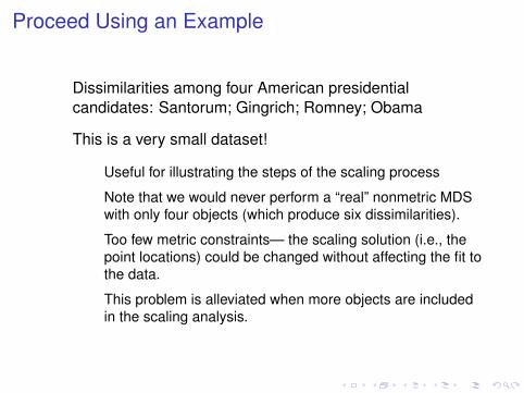
Proceed Using an Example
Dissimilarities among four American presidentialcandidates: Santorum; Gingrich; Romney; Obama
This is a very small dataset!
Useful for illustrating the steps of the scaling process
Note that we would never perform a “real” nonmetric MDSwith only four objects (which produce six dissimilarities).
Too few metric constraints— the scaling solution (i.e., thepoint locations) could be changed without affecting the fit tothe data.
This problem is alleviated when more objects are includedin the scaling analysis.
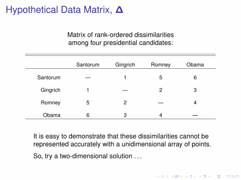
Hypothetical Data Matrix, ∆
Matrix of rank-ordered dissimilaritiesamong four presidential candidates:
Santorum Gingrich Romney Obama
Santorum — 1 5 6
Gingrich 1 — 2 3
Romney 5 2 — 4
Obama 6 3 4 —
It is easy to demonstrate that these dissimilarities cannot berepresented accurately with a unidimensional array of points.
So, try a two-dimensional solution . . .
Strategy for Nonmetric MDS
Start with random configuration of points intwo-dimensional space
We do not take this configuration seriously as a scalingsolution; it just provides a “neutral starting position.”
Use Pythagorean formula to calculate distances betweenpoints in the random configuration
Distances should be monotonic to dissimilarities data, butthey probably are not.
Move points around to create a new configuration that iscloser to the objective of a monotonic relationship betweendissimilarities and distances
Want to be as efficient with movements as possible— nounnecessary movements.
Distances and Disparities
Create a set of “target distances” that can be compared tocurrent actual distances in order to guide point movements
These target distances are called “disparities” in the MDSliterature
There is a disparity (target distance) associated with eachdistance between a pair of points.
The disparity associated with distance dij is designated d̂ij .
The disparities guide the point movements
If two points are too close together, then the disparity will belarger than the current distance (i.e., d̂ij > dij ); if they aretoo far apart, then the disparity will be smaller than thecurrent distance (i.e., d̂ij < dij )
Properties of Disparities
Disparities are characterized by two important properties:
1. Disparities are as similar to the actual distances as possible
That is, the correlation between the distances and thedisparities (rdij d̂ij
) is maximized.
2. Disparities are always monotonic to dissimilarities, even ifthe associated distances are not.
That is, if δij < δil then d̂ij ≤ d̂il , even if dij > dil
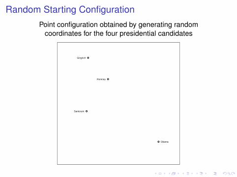
Random Starting ConfigurationPoint configuration obtained by generating random
coordinates for the four presidential candidates
●
●
●
●
Santorum
Gingrich
Romney
Obama
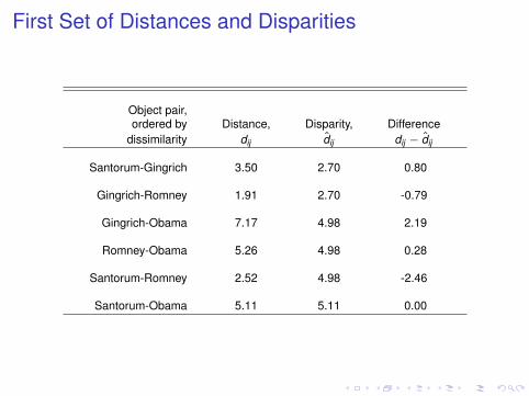
First Set of Distances and Disparities
Object pair,ordered by Distance, Disparity, Difference
dissimilarity dij d̂ij dij − d̂ij
Santorum-Gingrich 3.50 2.70 0.80
Gingrich-Romney 1.91 2.70 -0.79
Gingrich-Obama 7.17 4.98 2.19
Romney-Obama 5.26 4.98 0.28
Santorum-Romney 2.52 4.98 -2.46
Santorum-Obama 5.11 5.11 0.00
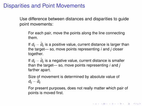
Disparities and Point Movements
Use difference between distances and disparities to guidepoint movements:
For each pair, move the points along the line connectingthem.
If dij − d̂ij is a positive value, current distance is larger thanthe target— so, move points representing i and j closertogether.
If dij − d̂ij is a negative value, current distance is smallerthan the target— so, move points representing i and jfarther apart.
Size of movement is determined by absolute value ofdij − d̂ij
For present purposes, does not really matter which pair ofpoints is moved first.

Second Point ConfigurationPoint configuration obtained after making first set of
moves, based upon previously-calculated disparities:
●
●
●
●
Santorum
Gingrich
Romney
Obama
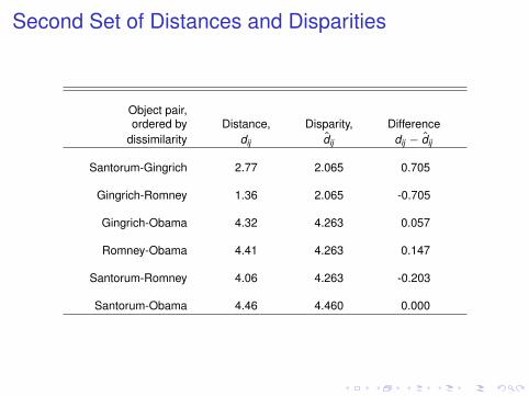
Second Set of Distances and Disparities
Object pair,ordered by Distance, Disparity, Difference
dissimilarity dij d̂ij dij − d̂ij
Santorum-Gingrich 2.77 2.065 0.705
Gingrich-Romney 1.36 2.065 -0.705
Gingrich-Obama 4.32 4.263 0.057
Romney-Obama 4.41 4.263 0.147
Santorum-Romney 4.06 4.263 -0.203
Santorum-Obama 4.46 4.460 0.000

Third Point ConfigurationPoint configuration obtained after making second set ofmoves, based upon second set of calculated disparities:
●
●
●
●
Santorum
Gingrich
Romney
Obama
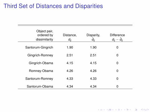
Third Set of Distances and Disparities
Object pair,ordered by Distance, Disparity, Difference
dissimilarity dij d̂ij dij − d̂ij
Santorum-Gingrich 1.90 1.90 0
Gingrich-Romney 2.51 2.51 0
Gingrich-Obama 4.15 4.15 0
Romney-Obama 4.26 4.26 0
Santorum-Romney 4.33 4.33 0
Santorum-Obama 4.34 4.34 0

Final Nonmetric MDS Solution
With the third set of points, the disparities are always equalto the actual interpoint distances
The distances are monotonic to the ordinal dissimilarities
There is no reason to carry out further point movements
The objective of the nonmetric MDS has been achieved
This solution fits data perfectly
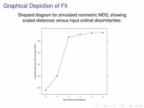
Graphical Depiction of FitShepard diagram for simulated nonmetric MDS, showing
scaled distances versus input ordinal dissimilarities:
Input ordinal dissimilarities
Inte
rpoi
nt d
ista
nces
from
non
met
ric M
DS
2.0
2.5
3.0
3.5
4.0
1 2 3 4 5 6

Need for a Measure of Fit
Perfect fit in scaling solution really only due to artificialnature of problem
Problematic, because too few metric constraints in data tocreate sufficiently stable scaling solution
Using nonmetric MDS on “real” data
More objects to be scaled
More difficult to obtain a perfect solution
But, often can reach a very good solution
Need to develop a fit measure that provides a summary ofdegree to which a nonmetric MDS solution achieves itsanalytic objective

Fit Statistic for Nonmetric MDS
Logic:
Want distances to be monotonic to dissimilarities
Disparities are as close to distances as possible, but alsomonotonic to dissimilarities
So, develop a measure that summarizes how different thedistances are from the disparities
Kruskal’s Stress1 coefficient:
Stress1 =
#pairs∑
i 6=j(dij − d̂ij)
2
#pairs∑i 6=j
d2ij
0.5
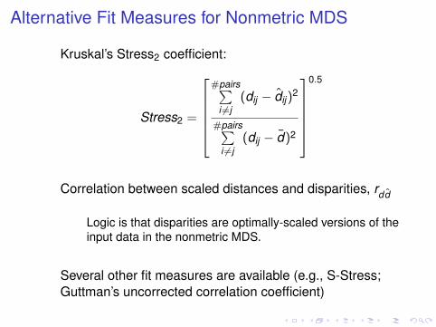
Alternative Fit Measures for Nonmetric MDS
Kruskal’s Stress2 coefficient:
Stress2 =
#pairs∑
i 6=j(dij − d̂ij)
2
#pairs∑i 6=j
(dij − d̄)2
0.5
Correlation between scaled distances and disparities, rdd̂
Logic is that disparities are optimally-scaled versions of theinput data in the nonmetric MDS.
Several other fit measures are available (e.g., S-Stress;Guttman’s uncorrected correlation coefficient)

Procedure for a “Real” Nonmetric MDS Routine
The value of the Stress coefficient is a function of the pointcoordinates in the current configuration (which are used tocalculate the distances and, indirectly, the disparities).
Therefore, can calculate the partial derivatives of Stress,relative to the coordinates:
∂Stress1
∂xip
For i = 1,2, . . . , k and p = 1,2, . . . ,m
Partial derivatives show how Stress changes when pointcoordinates are changed by a minute amount
Therefore, change point coordinates in ways that make thepartial derivatives the smallest possible negative values.
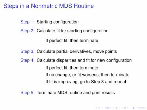
Steps in a Nonmetric MDS Routine
Step 1: Starting configuration
Step 2: Calculate fit for starting configuration
If perfect fit, then terminate
Step 3: Calculate partial derivatives, move points
Step 4: Calculate disparities and fit for new configuration
If perfect fit, then terminate
If no change, or fit worsens, then terminate
If fit is improving, go to Step 3 and repeat
Step 5: Terminate MDS routine and print results
Input Data for Nonmetric MDS Example
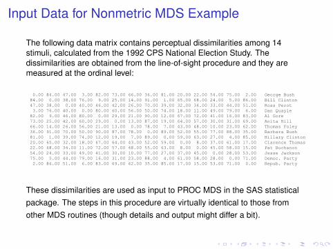
The following data matrix contains perceptual dissimilarities among 14stimuli, calculated from the 1992 CPS National Election Study. Thedissimilarities are obtained from the line-of-sight procedure and they aremeasured at the ordinal level:
Table 9: Input data for nonmetric multidimensional scaling
The following data matrix contains information from the 1992 CPS National Election Study. It is a square,symmetric matrix showing the electorate's perceived dissimilarities between each of the fourteen stimulidescribed below. The data are obtained from the line-of-sight procedure, and they are measured at the ordinallevel.
0.00 84.00 47.00 3.00 82.00 73.00 66.00 36.00 81.00 20.00 22.00 54.00 75.00 2.00 George Bush 84.00 0.00 38.00 76.00 9.00 25.00 14.00 91.00 1.00 65.00 68.00 24.00 5.00 86.00 Bill Clinton 47.00 38.00 0.00 40.00 46.00 42.00 26.00 70.00 39.00 32.00 34.00 33.00 44.00 51.00 Ross Perot 3.00 76.00 40.00 0.00 80.00 60.00 56.00 50.00 74.00 18.00 11.00 49.00 79.00 6.00 Dan Quayle 82.00 9.00 46.00 80.00 0.00 29.00 21.00 90.00 12.00 67.00 72.00 41.00 16.00 83.00 Al Gore 73.00 25.00 42.00 60.00 29.00 0.00 13.00 87.00 19.00 64.00 57.00 30.00 31.00 69.00 Anita Hill 66.00 14.00 26.00 56.00 21.00 13.00 0.00 78.00 7.00 43.00 48.00 10.00 23.00 62.00 Thomas Foley 36.00 91.00 70.00 50.00 90.00 87.00 78.00 0.00 89.00 52.00 55.00 77.00 88.00 35.00 Barbara Bush 81.00 1.00 39.00 74.00 12.00 19.00 7.00 89.00 0.00 59.00 63.00 27.00 4.00 85.00 Hillary Clinton 20.00 65.00 32.00 18.00 67.00 64.00 43.00 52.00 59.00 0.00 8.00 37.00 61.00 17.00 Clarence Thomas 22.00 68.00 34.00 11.00 72.00 57.00 48.00 55.00 63.00 8.00 0.00 45.00 58.00 15.00 Pat Buchanon 54.00 24.00 33.00 49.00 41.00 30.00 10.00 77.00 27.00 37.00 45.00 0.00 28.00 53.00 Jesse Jackson 75.00 5.00 44.00 79.00 16.00 31.00 23.00 88.00 4.00 61.00 58.00 28.00 0.00 71.00 Democ. Party 2.00 86.00 51.00 6.00 83.00 69.00 62.00 35.00 85.00 17.00 15.00 53.00 71.00 0.00 Repub. Party
The preceding dissimilarities matrix is used as input to PROC MDS in the SAS statistical package. Note thatthe steps in this procedure are virtually identical to those that would be produced by MDS routines in mostother statistical packages (although the details might differ a bit).These dissimilarities are used as input to PROC MDS in the SAS statisticalpackage. The steps in this procedure are virtually identical to those fromother MDS routines (though details and output might differ a bit).
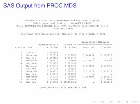
SAS Output from PROC MDS
Nonmetric MDS of 1992 Candidates and Political FiguresMultidimensional Scaling: Data=WORK.CAND92
Shape=TRIANGLE Cond=MATRIX Level=ORDINAL UNTIE Coef=IDENTITY Dim=2Formula=1 Fit=1
Mconverge=0.01 Gconverge=0.01 Maxiter=100 Over=2 Ridge=0.0001
Convergence MeasuresBadness-of-Fit Change in -------------------------
Iteration Type Criterion Criterion Monotone Gradient------------------------------------------------------------------------
0 Initial 0.108466 . . .1 Monotone 0.072379 0.036086 0.064224 0.5839702 Gau-New 0.057607 0.014772 . .3 Monotone 0.053911 0.003696 0.018435 0.2990024 Gau-New 0.052272 0.001639 . .5 Monotone 0.047879 0.004393 0.019191 0.2075586 Gau-New 0.047028 0.000851 . .7 Monotone 0.045217 0.001811 0.012829 0.1553768 Gau-New 0.044913 0.000304 . .9 Monotone 0.044012 0.000901 0.008895 0.10513210 Gau-New 0.043765 0.000247 . 0.01680611 Gau-New 0.043758 0.000006436 . 0.005644
Convergence criteria are satisfied.
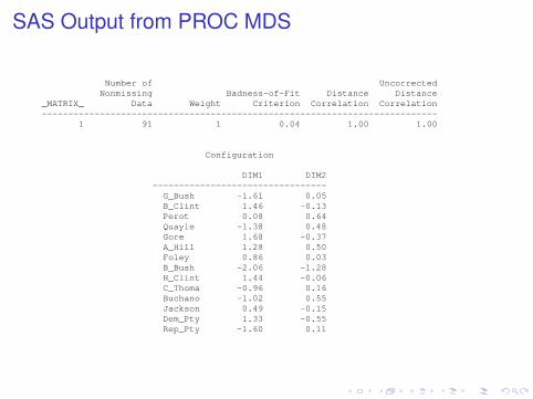
SAS Output from PROC MDS
Number of UncorrectedNonmissing Badness-of-Fit Distance Distance
_MATRIX_ Data Weight Criterion Correlation Correlation---------------------------------------------------------------------------
1 91 1 0.04 1.00 1.00
Configuration
DIM1 DIM2---------------------------------G_Bush -1.61 0.05B_Clint 1.46 -0.13Perot 0.08 0.64Quayle -1.38 0.48Gore 1.68 -0.37A_Hill 1.28 0.50Foley 0.86 0.03B_Bush -2.06 -1.28H_Clint 1.44 -0.06C_Thoma -0.96 0.16Buchano -1.02 0.55Jackson 0.49 -0.15Dem_Pty 1.33 -0.55Rep_Pty -1.60 0.11
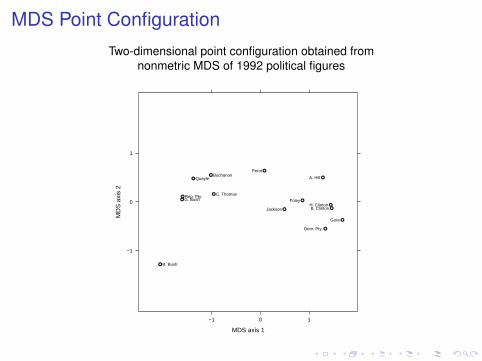
MDS Point ConfigurationTwo-dimensional point configuration obtained from
nonmetric MDS of 1992 political figures
MDS axis 1
MD
S a
xis
2
−1
0
1
−1 0 1
●
●
●
●
●
●
●
●
●
●
●
●
●
●G. Bush
Quayle
B. Bush
C. Thomas
Buchanon
Rep. Pty.
B. Clinton
Perot
Gore
A. Hill
FoleyH. Clinton
Jackson
Dem. Pty.
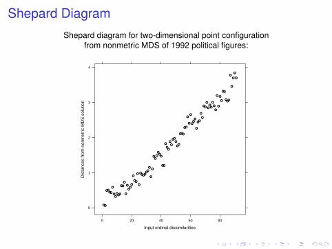
Shepard DiagramShepard diagram for two-dimensional point configuration
from nonmetric MDS of 1992 political figures:
Input ordinal dissimilarities
Dis
tanc
es fr
om n
onm
etric
MD
S s
olut
ion
0
1
2
3
4
0 20 40 60 80
●
●
●
●
●
●
●
●
●
●
●
●
●
●
●
●
●
●
●
●
●
●
●
●
●
●●
●
●
●
●
●
●
●●
●
●
●
●
●
●
●
● ●
●
●
●
●
●
●
●
●
●
●
●
●
●
●
●
●
●
●
●
●
●
●
●
●
●
●
●
●
●
●
●
●
●
●
●
●
●
●
●
●
●
●
●
●
●
●
●
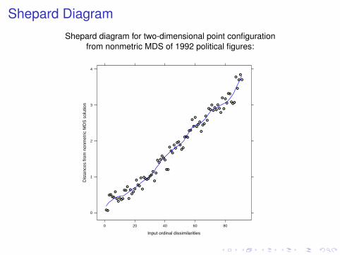
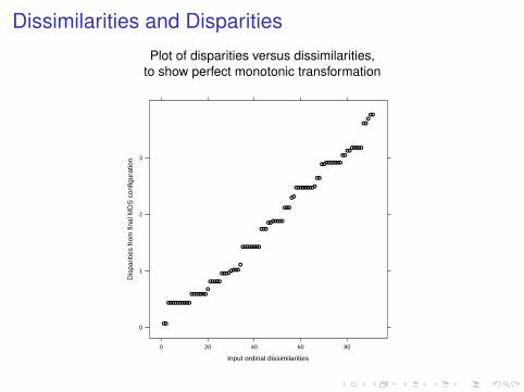
Dissimilarities and DisparitiesPlot of disparities versus dissimilarities,
to show perfect monotonic transformation
Input ordinal dissimilarities
Dis
parit
ies
from
fina
l MD
S c
onfig
urat
ion
0
1
2
3
0 20 40 60 80
●
●
●
●
●
●
●
●
●
●
●
●
●
●
●
●
●
●
●
●
●
●
●
●
●
●
●
●●
●
●
●
●
●
●
●
●
●
●
●
●
●
●
●
●
●
●
●
●
●
●
●
●
●
●
●
●
●
●
●
●
●
●
●
●
●
●
●
●
●
●
●
●
●
●
●●
●
●
●
●
●
●
●
●
●
●
●●
●
●

Interpreting an MDS Solution
Metric and nonmetric versions of CMDS only determinerelative distances between points in scaled m-space
The locations of the coordinate axes for the pointconfiguration are completely arbitrary
Final MDS point configuration usually rotated to a “varimax”orientation
Point coordinates usually standardized to a mean of zeroon each axis and a variance of 1.0 (or some other specifiedvalue)
Axes have no intrinsic substantive importance orinterpretation!

Interpretation Strategies for MDS
Generally, try to look for two kinds of structure in an MDSsolution:
Interesting directions within the m-space
A direction would usually be “interesting” if points that fall atopposite sides of the space correspond to objects that arecontrasting with respect to some substantive characteristic
Interesting groups of points within the m-space
A grouping of points would be “interesting” if the objectscorresponding to the grouped points are differentiated fromthe other objects in terms of some recognizable substantivecharacteristic
Of course, both kinds of structure can occursimultaneously, within a single MDS solution.
Some Cautions About Interpretation
Simplicity of underlying model and potential for graphicalrepresentation of scaling results both facilitateinterpretation
For many purposes, simply “eyeballing” the pointconfiguration is sufficient for interpretation
But, visual interpretation has potential limitations:
It is much more difficult when m > 2, and almost impossiblewhen m > 3.
Highly subjective— we may see structured patterns that arenot really there
For these reasons, it is useful to employ more systematicmethods for interpreting an MDS solution

Embedding External Variables
Researcher often has prior hypotheses about dimensionsthat differentiate objects in MDS analysis
Useful to obtain “external” measures of the objects alongthese dimensions, separate from the data employed for theMDS
If point configuration really does conform to variability ofthe objects along the external criterion variable, then wecan embed an axis representing that dimension within theMDS space
Simple regression procedure for doing so . . .

Embedding External Criterion Variables
Assume an external variable, Y , is available:
Each of the k objects in the MDS have scores on theexternal variable, y1, y2, . . . , yk .
Regress Y on the MDS coordinate axes (Dim1, Dim2, . . . ,Dimk ):
yi = α + β1 Dim1i + β2 Dim2i + . . .+ βk Dimki + ei
If regression equation fits well (i.e., R2 is large), then Y isconsistent with the spatial configuration of objects
Inserting External Variable into MDS Space
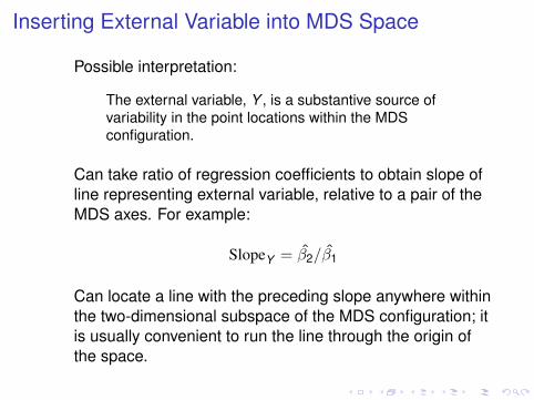
Possible interpretation:
The external variable, Y , is a substantive source ofvariability in the point locations within the MDSconfiguration.
Can take ratio of regression coefficients to obtain slope ofline representing external variable, relative to a pair of theMDS axes. For example:
SlopeY = β̂2/β̂1
Can locate a line with the preceding slope anywhere withinthe two-dimensional subspace of the MDS configuration; itis usually convenient to run the line through the origin ofthe space.
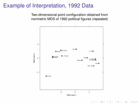
Example of Interpretation, 1992 DataTwo-dimensional point configuration obtained fromnonmetric MDS of 1992 political figures (repeated)
MDS axis 1
MD
S a
xis
2
−1
0
1
−1 0 1
●
●
●
●
●
●
●
●
●
●
●
●
●
●G. Bush
Quayle
B. Bush
C. Thomas
Buchanon
Rep. Pty.
B. Clinton
Perot
Gore
A. Hill
FoleyH. Clinton
Jackson
Dem. Pty.
Theoretical Predictions
Public perceptions of political figures are affected by twofactors:
Ideology
Overall popularity
Operationalize the two variables:
LC: A scale ranging from -100 to 100, with negative valuesindicating liberal positions, positive values indicatingconservative positions
AFF: A 0-100 scale, with larger values corresponding togreater popularity

Data Matrix with External Variables
Table 10: External criteria for interpreting directions within the MDS solution.
Substantive theory suggests that citizens' perceptions of political figures are affected by at least two factors: Thepopularity of each political figure, and the ideology usually associated with that political figure. Are the nonmetricmultidimensional scaling results from the 1992 NES consistent with this theoretical perspective? In order to testthese hypotheses, we obtain information on the overall popularity and the perceived ideological position of eachof the scaled political figures. In the data shown below, the variables D1 and D2 are the coordinate axes obtainedfrom the MDS analysis. The variable AFFECT measures popularity (on a 0-100 scale, with higher valuesindicating greater public approval) and LC measures perceived ideological position (with negative valuesindicating more liberal positions, and positive values showing relatively conservative positions).
D1: D2: AFFECT: LC: NAME: -1.61 0.05 52 27 G. Bush 1.46 -0.13 56 -22 B. Clinton 0.08 0.64 45 0 Perot -1.38 0.48 42 29 Quayle 1.68 -0.37 57 -18 Gore 1.28 0.50 49 -19 A. Hill 0.86 0.03 48 -9 Foley -2.06 -1.28 67 12 B. Bush 1.44 -0.06 54 -17 H. Clinton -0.96 0.16 45 15 C. Thomas -1.02 0.55 42 19 Buchanon 0.49 -0.15 47 -16 Jackson 1.33 -0.55 59 -19 Dem. Pty. -1.60 0.11 52 22 Rep. Pty.

OLS Estimates for Ideology, 1992 Data
Ideology equation:
LCi = 0.289− 13.343 Dim1i + 8.657 Dim2i + ei
R2 = 0.940
SlopeLC = 8.657−13.343 = −0.649
Draw line representing ideology dimension into configuration

Inserting Ideology Dimension
Two-dimensional point configuration withliberal-conservative dimension inserted
MDS axis 1
MD
S a
xis
2
−1
0
1
−1 0 1
●
●
●
●
●
●
●
●
●
●
●
●
●
●G. Bush
Quayle
B. Bush
C. Thomas
Buchanon
Rep. Pty.
B. Clinton
Perot
Gore
A. Hill
FoleyH. Clinton
Jackson
Dem. Pty.
Lib−Con Dimension

OLS Estimates for Popularity, 1992 Data
Popularity equation:
AFFi = 51.054 + 0.655 Dim1i − 12.622 Dim2i + ei
R2 = 0.832
SlopeAFF = −12.6220.655 = −19.270
Draw line representing popularity dimension into configuration
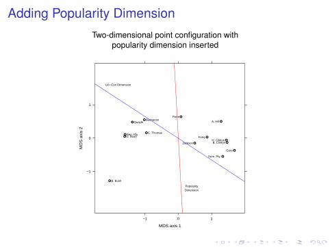
Adding Popularity DimensionTwo-dimensional point configuration with
popularity dimension inserted
MDS axis 1
MD
S a
xis
2
−1
0
1
−1 0 1
●
●
●
●
●
●
●
●
●
●
●
●
●
●G. Bush
Quayle
B. Bush
C. Thomas
Buchanon
Rep. Pty.
B. Clinton
Perot
Gore
A. Hill
FoleyH. Clinton
Jackson
Dem. Pty.
Lib−Con Dimension
PopularityDimension
Finding Groups of Points in MDS Solution
Cluster analysis is a family of methods for creatingtaxonomies of objects
Divides objects into a set of (usually) mutually exclusivecategories
Objects that are close to each other are placed into acommon cluster; more distant objects are placed intodifferent clusters.
There are many varieties of cluster analysis

Hierarchical Cluster Analysis
Begin with each object in a separate cluster
Proceed through k − 1 steps, creating a new cluster oneach step
On each step, join together the two closest clusters
The location of each new cluster is (usually) the meanlocation of the objects contained in the cluster
At the k − 1 step, all objects are joined in a common cluster
Diagram called the “dendrogram” traces the steps of theclustering process.
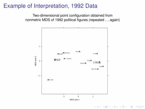
Example of Interpretation, 1992 DataTwo-dimensional point configuration obtained from
nonmetric MDS of 1992 political figures (repeated . . . again)
MDS axis 1
MD
S a
xis
2
−1
0
1
−1 0 1
●
●
●
●
●
●
●
●
●
●
●
●
●
●G. Bush
Quayle
B. Bush
C. Thomas
Buchanon
Rep. Pty.
B. Clinton
Perot
Gore
A. Hill
FoleyH. Clinton
Jackson
Dem. Pty.

Cluster Analysis of 1992 MDS Solution
Dendrogram from hierarchical cluster analysis:
Dendrogram for MDS_92 cluster analysis
L2 d
issi
mila
rity
mea
sure
0
2.60935
G R Q B C B B H G D A F J PB e u u T _ C C o e H o a eu p a c h B l l r m i l c rs P y h o u i i e P l e k oh t l a m s n n t l y s t
y e n a h t t y oo n
Figure 15: Dendrogram for hierarchical cluster analysis of two-dimensional point configuration obtained fromnonmetric MDS of 1992 political figures.

More Caveats about Interpretation
Most MDS solutions are amenable to several differentsubstantive solutions
Objective strategies (i.e., external variables, clusteranalysis) can show that scaling results are consistent withsome particular interpretation
Objective methods can never be used to find the single,“true” meaning of an MDS point configuration
This apparent uncertainty bothers some researchers . . .
MDS and Scientific Theories
In fact, the tentative nature of an MDS interpretation is nodifferent from the general process of scientific theoryconstruction and testing:
The analyst demonstrates that the empirical data (MDSsolution, in this case) are consistent with a specific story(i.e., a theory)
The story becomes the accepted version of reality . . .
Until someone demonstrates that another story (i.e.,theory) provides a better description of the same data.

Data for MDS
Direct dissimilarity judgments about stimuli
Physical distances
Profile dissimilarities (sum-of-squared differencemeasures)
Confusion measures
Temporal change rates
LOS dissimilarities
Correlations (problematic)
Potential Problems with MDS
Too few stimuli in nonmetric MDS
Local minima
Degenerate solutions
Nonstandardized terminology
MDS usually regarded as data analytic procedure, not astatistical model