Download - MRFs and Segmentation with Graph Cuts

MRFs and Segmentation with Graph Cuts
Computer VisionCS 543 / ECE 549
University of Illinois
Derek Hoiem
02/24/10

Today’s class
• Finish up EM
• MRFs
• Segmentation with Graph Cuts
i
j
wij

EM Algorithm: Recap
1. E-step: compute
2. M-step: solve
• Determines hidden variable assignments and parameters that maximize likelihood of observed data
• Improves likelihood at each step (reaches local maximum)• Derivation is tricky but implementation is easy
)(,|
,||,log|,logE )(t
xzpppt
xzzxzx
z
)()1( ,||,logargmax tt pp
xzzxz
EM Demos
• Mixture of Gaussian demo
• Simple segmentation demo

“Hard EM”• Same as EM except compute z* as most likely
values for hidden variables
• K-means is an example
• Advantages– Simpler: can be applied when cannot derive EM– Sometimes works better if you want to make hard
predictions at the end• But
– Generally, pdf parameters are not as accurate as EM

Missing Data Problems: OutliersYou want to train an algorithm to predict whether a photograph is attractive. You collect annotations from Mechanical Turk. Some annotators try to give accurate ratings, but others answer randomly.
Challenge: Determine which people to trust and the average rating by accurate annotators.
Photo: Jam343 (Flickr)
Annotator Ratings
108928

Missing Data Problems: Object Discovery
You have a collection of images and have extracted regions from them. Each is represented by a histogram of “visual words”.
Challenge: Discover frequently occurring object categories, without pre-trained appearance models.
http://www.robots.ox.ac.uk/~vgg/publications/papers/russell06.pdf

n is the total count of the histogram

What’s wrong with this prediction?
P(foreground | image)

Solution
P(foreground | image)
Encode dependencies between pixels
edgesji
jiNi
i datayyfdatayfZ
dataP,
2..1
1 ),;,(),;(1
),;( y
Labels to be predicted Individual predictions Pairwise predictions
Normalizing constant

Writing Likelihood as an “Energy”
edgesji
jiNi
i datayypdataypZ
dataP,
2..1
1 ),;,(),;(1
),;( y
edgesji
jii
i datayydataydataEnergy,
21 ),;,(),;(),;( y
“Cost” of assignment yi
“Cost” of pairwise assignment yi ,yj

Markov Random Fields
edgesji
jii
i datayydataydataEnergy,
21 ),;,(),;(),;( y
Node yi: pixel label
Edge: constrained pairs
Cost to assign a label to each pixel
Cost to assign a pair of labels to connected pixels

Markov Random Fields
• Example: “label smoothing” gridUnary potential
0 10 0 K1 K 0
Pairwise Potential
0: -logP(yi = 0 ; data)1: -logP(yi = 1 ; data)
edgesji
jii
i datayydataydataEnergy,
21 ),;,(),;(),;( y
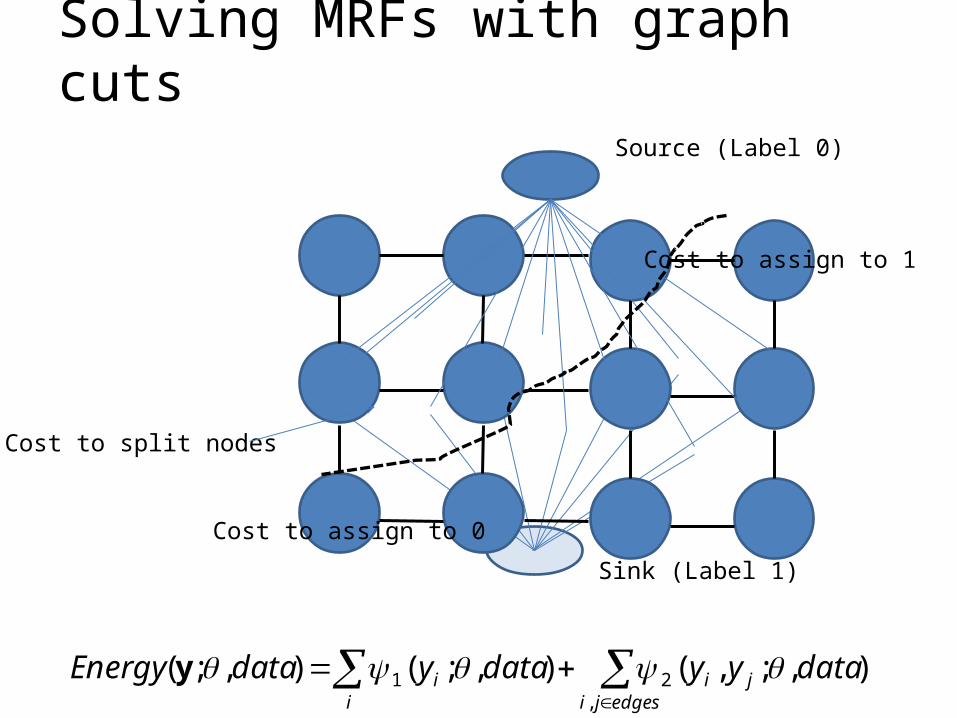
Solving MRFs with graph cuts
edgesji
jii
i datayydataydataEnergy,
21 ),;,(),;(),;( y
Source (Label 0)
Sink (Label 1)
Cost to assign to 1
Cost to assign to 0
Cost to split nodes

Solving MRFs with graph cuts
edgesji
jii
i datayydataydataEnergy,
21 ),;,(),;(),;( y
Source (Label 0)
Sink (Label 1)
Cost to assign to 0
Cost to assign to 1
Cost to split nodes

GrabCut segmentation
User provides rough indication of foreground region.
Goal: Automatically provide a pixel-level segmentation.

Grab cuts and graph cuts Grab cuts and graph cuts
User Input
Result
Magic Wand (198?)
Intelligent ScissorsMortensen and Barrett (1995)
GrabCut
Regions Boundary Regions & Boundary
Source: Rother

Colour Model Colour Model
Gaussian Mixture Model (typically 5-8 components)
Foreground &Background
Background G
R
Source: Rother

Graph cuts Boykov and Jolly (2001)
Graph cuts Boykov and Jolly (2001)
Image Min Cut
Cut: separating source and sink; Energy: collection of edges
Min Cut: Global minimal enegry in polynomial time
Foreground (source)
Background(sink)
Source: Rother

Colour Model Colour Model
Gaussian Mixture Model (typically 5-8 components)
Foreground &Background
Background
Foreground
BackgroundG
R
G
RIterated graph cut
Source: Rother

GrabCut segmentation
1. Define graph – usually 4-connected or 8-connected
2. Define unary potentials– Color histogram or mixture of Gaussians for
background and foreground
3. Define pairwise potentials
4. Apply graph cuts5. Return to 2, using current labels to compute
foreground, background models
2
2
21 2
)()(exp),(_
ycxc
kkyxpotentialedge
));((
));((log)(_
background
foreground
xcP
xcPxpotentialunary

What is easy or hard about these cases for graphcut-based segmentation?

Easier examples
GrabCut – Interactive Foreground Extraction 10

More difficult Examples
Camouflage & Low Contrast Harder CaseFine structure
Initial Rectangle
InitialResult
GrabCut – Interactive Foreground Extraction 11


Lazy Snapping (Li et al. SG 2004)

Using graph cuts for recognition
TextonBoost (Shotton et al. 2009 IJCV)

Using graph cuts for recognition
TextonBoost (Shotton et al. 2009 IJCV)
Unary Potentials
Alpha Expansion Graph Cuts

Limitations of graph cuts
• Associative: edge potentials penalize different labels
• If not associative, can sometimes clip potentials
• Approximate for multilabel– Alpha-expansion or alpha-beta swaps
Must satisfy

Graph cuts: Pros and Cons• Pros
– Very fast inference– Can incorporate data likelihoods and priors– Applies to a wide range of problems (stereo,
image labeling, recognition)• Cons
– Not always applicable (associative only)– Need unary terms (not used for generic
segmentation)• Use whenever applicable

More about MRFs/CRFs
• Other common uses– Graph structure on regions– Encoding relations between multiple scene
elements
• Inference methods– Loopy BP or BP-TRW: approximate, slower, but
works for more general graphs

Further reading and resources
• Graph cuts– http://www.cs.cornell.edu/~rdz/graphcuts.html– Classic paper: What Energy Functions can be Minimized via Graph Cuts?
(Kolmogorov and Zabih, ECCV '02/PAMI '04)
• Belief propagationYedidia, J.S.; Freeman, W.T.; Weiss, Y., "Understanding Belief Propagation and Its Generalizations”, Technical Report, 2001: http://www.merl.com/publications/TR2001-022/
• Normalized cuts and image segmentation (Shi and Malik)http://www.cs.berkeley.edu/~malik/papers/SM-ncut.pdf
• N-cut implementation http://www.seas.upenn.edu/~timothee/software/ncut/ncut.html

Next Class• Gestalt grouping
• More segmentation methods


