
AGRODEP Stata Training documents are designed to give AGRODEP members a brief overview of
basic Stata commands needed in AGRODEP training courses. These documents have been reviewed but
have not been subject to a formal external peer review via IFPRI’s Publications Review Committee; any
opinions expressed are those of the author(s) and do not necessarily reflect the opinions of AGRODEP or
of IFPRI.
AGRODEP Stata Training
April 2013
Module 1
Introduction to Stata
Manuel Barron1 and Pia Basurto
2
1 University of California, Berkeley, Department of Agricultural and Resource Economics
2 University of California, Santa Cruz, Department of Economics
1
Module 1 – Introduction to Stata
1. Introduction
These notes are designed for AGRODEP members with little prior experience using Stata. Stata is a
statistical processing package that can be used for data management and to perform statistical analysis.
This tutorial will provide background information and introduce you to commands that will be necessary
in AGRODEP training courses. Please note that the information presented here is about Stata and not
about econometrics. We will not discuss statistical properties or parameter interpretation; we will focus
on presenting the basic commands that you will need to use for those tasks. The topics covered in
AGRODEP training courses may require some advanced commands not presented in this tutorial. Those
details will be covered by the course instructor.
2. Getting Started
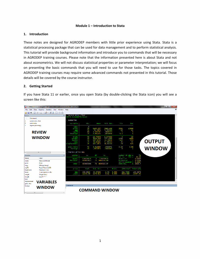
If you have Stata 11 or earlier, once you open Stata (by double-clicking the Stata icon) you will see a
screen like this:
2
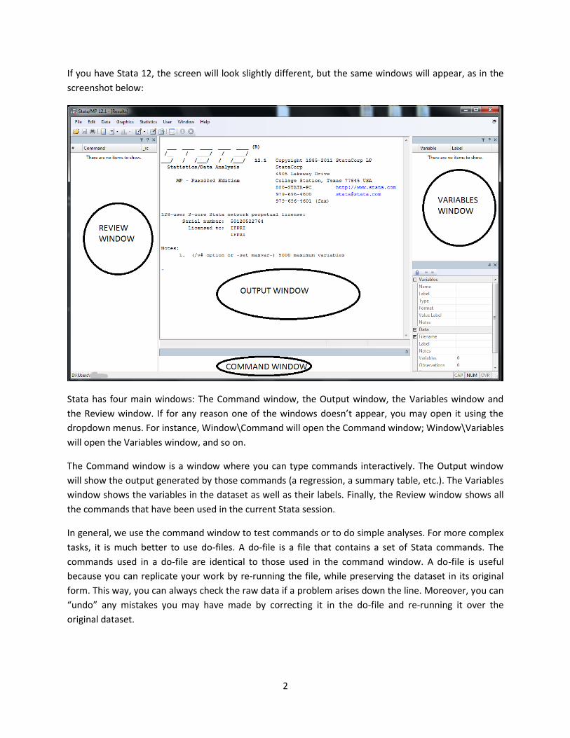
If you have Stata 12, the screen will look slightly different, but the same windows will appear, as in the
screenshot below:
Stata has four main windows: The Command window, the Output window, the Variables window and
the Review window. If for any reason one of the windows doesn’t appear, you may open it using the
dropdown menus. For instance, Window\Command will open the Command window; Window\Variables
will open the Variables window, and so on.
The Command window is a window where you can type commands interactively. The Output window
will show the output generated by those commands (a regression, a summary table, etc.). The Variables
window shows the variables in the dataset as well as their labels. Finally, the Review window shows all
the commands that have been used in the current Stata session.
In general, we use the command window to test commands or to do simple analyses. For more complex
tasks, it is much better to use do-files. A do-file is a file that contains a set of Stata commands. The
commands used in a do-file are identical to those used in the command window. A do-file is useful
because you can replicate your work by re-running the file, while preserving the dataset in its original
form. This way, you can always check the raw data if a problem arises down the line. Moreover, you can
“undo” any mistakes you may have made by correcting it in the do-file and re-running it over the
original dataset.

3
To get started, we will use a dataset commonly used in Stata’s help files: the “auto.dta” dataset, which
contains information about automobiles. In these notes, the words in courier new font are
commands that you should type in the command window (or do-file). When we refer to commands in
the text, we will use italics.
In these notes we will use boxes like the one below to show commands in the Do-files or the Command
Window, results from the Output Window, or contents from Help files. The first line in the box will tell
you what the box represents. For instance, the box below refers to a command window. You don’t need
to type the line “* Command Window”, you just need to type the line “doedit”.
To open a do-file, click on the “New do-file editor” icon on the menu bar, or type doedit on the
Command Window.
* Command Window
doedit
The next figure shows what a do-file looks like. There are several icons at the top. The most important
ones are:
NEW: to open a new do-file
OPEN: to open an existing do-file
SAVE: to save the current do-file
DO or EXECUTE: to execute the commands
4
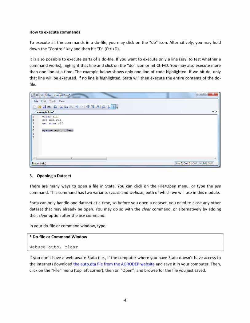
How to execute commands
To execute all the commands in a do-file, you may click on the “do” icon. Alternatively, you may hold
down the “Control” key and then hit “D” (Ctrl+D).
It is also possible to execute parts of a do-file. If you want to execute only a line (say, to test whether a
command works), highlight that line and click on the “do” icon or hit Ctrl+D. You may also execute more
than one line at a time. The example below shows only one line of code highlighted. If we hit do, only
that line will be executed. If no line is highlighted, Stata will then execute the entire contents of the do-
file.
3. Opening a Dataset
There are many ways to open a file in Stata. You can click on the File/Open menu, or type the use
command. This command has two variants sysuse and webuse, both of which we will use in this module.
Stata can only handle one dataset at a time, so before you open a dataset, you need to close any other
dataset that may already be open. You may do so with the clear command, or alternatively by adding
the , clear option after the use command.
In your do-file or command window, type:
* Do-file or Command Window
webuse auto, clear
If you don’t have a web-aware Stata (i.e., if the computer where you have Stata doesn’t have access to
the internet) download the auto.dta file from the AGRODEP website and save it in your computer. Then,
click on the “File” menu (top left corner), then on “Open”, and browse for the file you just saved.

5
You will see a line like the following in the Output window. In the Output Window, every line of
commands executed by Stata starts with a period. If you open the auto.dta file using the menus, you will
see the following output in the Output Window.
*Output Window
. use "C:\Users\Stata_Training\auto.dta", clear
(of course, instead of “C:\Users\Stata_Training\auto.dta” you will see the route in your own computer).
The command as it appeared in the output window would have opened the “auto.dta” dataset.
If your command contains an error, Stata will produce a red error message on the output screen. Error
messages can be specific. For instance, if we type ebuse instead of webuse, the error message will read:
“unrecognized command: ebuse”. This is quite specific, because it says there is a problem with the
command name. Other times, the error message may be much more general, for example: “syntax
error”. This means there is an error in the syntax, but Stata doesn’t point directly at what is causing the
problem.
If you run a do-file, any error will make it stop. You need to correct the error and run the do-file again.
This happens plenty of times every time anyone (even advanced users) use Stata or any other
programming language, so don’t get disappointed!
You can set a working directory with the cd command. Once you set the working directory, you may
refer to any file in that directory without writing the whole path in your do-file. Stata will know to look
for a file there, or to save your file in that directory. You may type cd in the command window to see
the current working directory. Setting a working directory is especially helpful when your do-file includes
more than one file, or when you use the outreg2 command to export your regression results to other
programs outside Stata (like Excel or Word).
* Do-file – not using cd
use "C:\Users\Stata_Training\auto.dta", clear
… more stata commands…
save "C:\Users\Stata_Training\auto_v2.dta", replace
* Do-file – using cd
cd "C:\Users\Stata_Training\"
use "auto.dta", clear
… more stata commands…
save "auto_v2.dta", replace

6
4. Logical operators: “and”, “or”, “if”, “not”
Before we start using commands, we should discuss logical operators. You can use the “if” logical
operator to perform an operation in a subset of observations that fulfill a certain condition. Let’s look at
an example.
*Do file or Command Window
count
count if foreign==1
The count command counts the total number of observations (i.e. the number of rows in a dataset). The
count if foreign==1 line counts the number of observations that have the value of foreign equal to one.
Note that Stata uses two equal signs after if. In general, Stata uses two equal signs if it is asked to
evaluate a value, and one equal sign if it is asked to alter a value. We will see more of this when we
discuss variable generation. Using an incorrect number of equal signs is one of the most common
mistakes when writing a Stata command. Always check that the number of signs is appropriate when
Stata produces an error message.
The following commands introduce four new operators: <, >, |, and &. The < and > operators mean “less
than” and “greater than”. When followed by a = operator, <= means “less than or equal to”, and >=
means “greater than or equal to”. In addition, | means “OR”, while & means “AND”.
*Do file or Command Window
count if weight<=2000 | weight>=4000
count if weight<2000 & weight>4000
Thus, the line count if weight<=2000 | weight>=40 counts the number of cars that weigh either less than
(or equal to) 2,000 pounds or more than (or equal to) 4,000 pounds. In the same way, the next line
counts the number of cars that weigh less than 2,000 pounds and more than 4,000 pounds. This last line
is a trick, since no car can possibly weigh less than 2,000 and more than 4,000 pounds at the same time.
Even though the second line makes no sense mathematically, Stata will return 0 rather than produce an
error, because there is no error in the syntax.
We can use more than one condition in an if statement. In these cases, we should use parentheses to
ensure that Stata understands the hierarchy of our conditions, in a similar way in which parentheses are
used in mathematics to indicate the order of operations.
*Do file or Command Window
count if (weight<=2000 & foreign==1) | foreign==0
This will count the number of cars that are either foreign and less than (or equal to) 2,000 pounds, or
not foreign (irrespective of their weight).
7
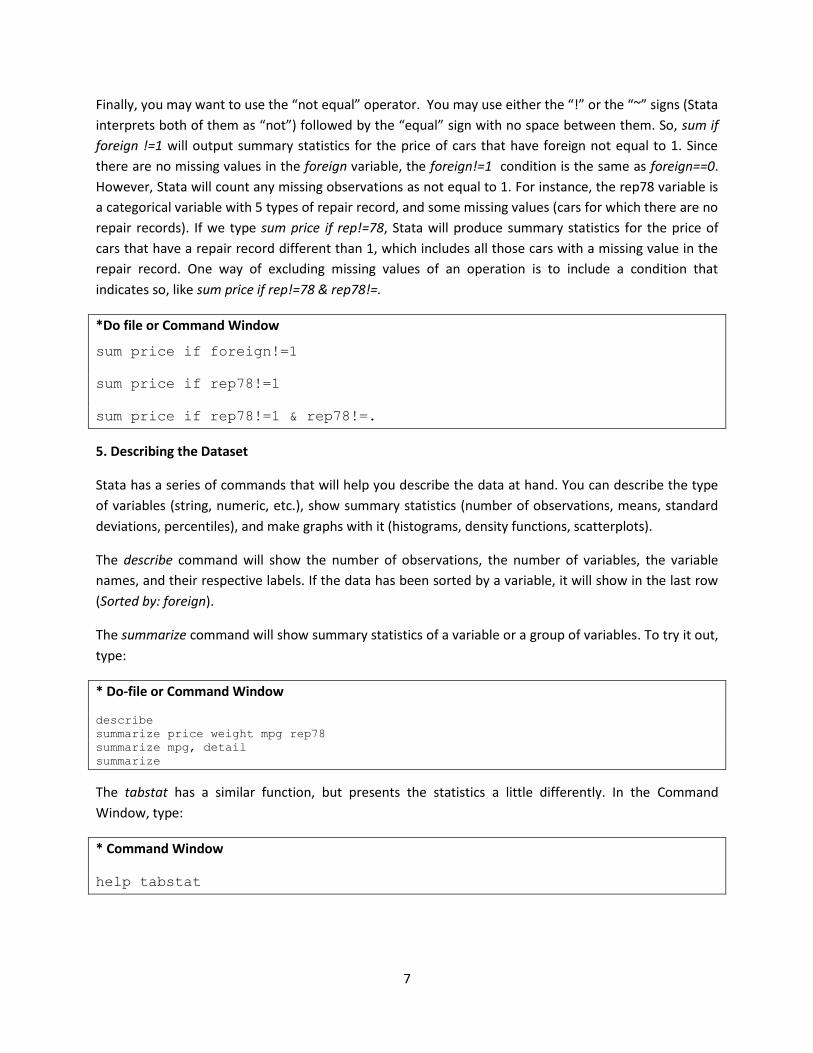
Finally, you may want to use the “not equal” operator. You may use either the “!” or the “~” signs (Stata
interprets both of them as “not”) followed by the “equal” sign with no space between them. So, sum if
foreign !=1 will output summary statistics for the price of cars that have foreign not equal to 1. Since
there are no missing values in the foreign variable, the foreign!=1 condition is the same as foreign==0.
However, Stata will count any missing observations as not equal to 1. For instance, the rep78 variable is
a categorical variable with 5 types of repair record, and some missing values (cars for which there are no
repair records). If we type sum price if rep!=78, Stata will produce summary statistics for the price of
cars that have a repair record different than 1, which includes all those cars with a missing value in the
repair record. One way of excluding missing values of an operation is to include a condition that
indicates so, like sum price if rep!=78 & rep78!=.
*Do file or Command Window
sum price if foreign!=1
sum price if rep78!=1
sum price if rep78!=1 & rep78!=.
5. Describing the Dataset
Stata has a series of commands that will help you describe the data at hand. You can describe the type
of variables (string, numeric, etc.), show summary statistics (number of observations, means, standard
deviations, percentiles), and make graphs with it (histograms, density functions, scatterplots).
The describe command will show the number of observations, the number of variables, the variable
names, and their respective labels. If the data has been sorted by a variable, it will show in the last row
(Sorted by: foreign).
The summarize command will show summary statistics of a variable or a group of variables. To try it out,
type:
* Do-file or Command Window
describe
summarize price weight mpg rep78
summarize mpg, detail
summarize
The tabstat has a similar function, but presents the statistics a little differently. In the Command
Window, type:
* Command Window
help tabstat
8
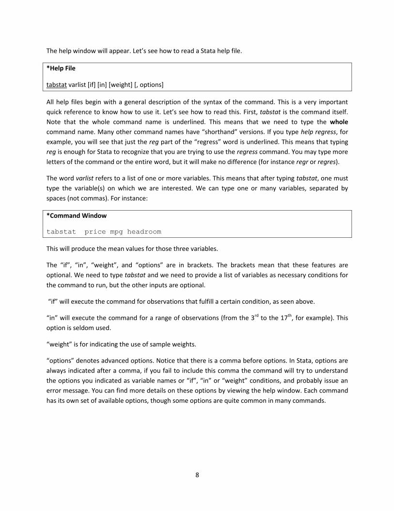
The help window will appear. Let’s see how to read a Stata help file.
*Help File
tabstat varlist [if] [in] [weight] [, options]
All help files begin with a general description of the syntax of the command. This is a very important
quick reference to know how to use it. Let’s see how to read this. First, tabstat is the command itself.
Note that the whole command name is underlined. This means that we need to type the whole
command name. Many other command names have “shorthand” versions. If you type help regress, for
example, you will see that just the reg part of the “regress” word is underlined. This means that typing
reg is enough for Stata to recognize that you are trying to use the regress command. You may type more
letters of the command or the entire word, but it will make no difference (for instance regr or regres).
The word varlist refers to a list of one or more variables. This means that after typing tabstat, one must
type the variable(s) on which we are interested. We can type one or many variables, separated by
spaces (not commas). For instance:
*Command Window
tabstat price mpg headroom
This will produce the mean values for those three variables.
The “if”, “in”, “weight”, and “options” are in brackets. The brackets mean that these features are
optional. We need to type tabstat and we need to provide a list of variables as necessary conditions for
the command to run, but the other inputs are optional.
“if” will execute the command for observations that fulfill a certain condition, as seen above.
“in” will execute the command for a range of observations (from the 3rd to the 17th, for example). This
option is seldom used.
“weight” is for indicating the use of sample weights.
“options” denotes advanced options. Notice that there is a comma before options. In Stata, options are
always indicated after a comma, if you fail to include this comma the command will try to understand
the options you indicated as variable names or “if”, “in” or “weight” conditions, and probably issue an
error message. You can find more details on these options by viewing the help window. Each command
has its own set of available options, though some options are quite common in many commands.

9
Let’s see how we can use this in an example. In your Do-File or Command Window, type:
*Do-file or Command Window
tabstat price mpg headroom if foreign==1
We just generated the means for the same variables, but only for the subset of foreign cars.
*Do-file or Command Window
tabstat price mpg headroom if price>6500
We just generated the means for the same variables, but only for expensive cars (those that cost more
than $6,500).
*Do-file or Command Window
tabstat price mpg headroom if price>6500 & foreign==0
This command generates the means for those same variables, for cars that are both expensive and
domestic.
In the tabstat command, the statistics option is pretty important. It tells us which statistics can be
calculated with tabstat. As you have seen, if you specify nothing, tabstat will report the mean value (this
is called a default option, and most commands have one predetermined). But tabstat can also report the
number of observations with valid data, the sum, maximum, minimum, range, standard deviation,
variance, coefficient of variation, the standard error of the mean, as well as several moments of the
distribution: the skewness, kurtosis, percentiles, and the interquartile range. For example,
* Do-file or Command Window
tabstat price mpg headroom if price>=6500, stats(mean sd p50 kurtosis)
would show the mean, the standard deviation, the median (50th percentile) and the kurtosis for the
price, miles per gallon (mpg) and headroom variables for the subset of expensive cars.
We can also present the results split by groups. In this case, we split the results between foreign and
domestic cars:
* Do-file or Command Window
tabstat price mpg headroom, stats(mean sd p50 kurtosis) by(foreign)
The statistics are reported in the order you put them in the command line. The first one is the mean, the
second line reports the standard deviation, the third line reports the 50th percentile (the median), and
the last line reports the kurtosis.

10
If you scroll down further in the help window, you will see more details about the command tabstat, and
at the very bottom you will see examples of how the command can be used. In the case of tabstat, the
examples are:
* Help File
Examples
Setup
. sysuse auto
Show the mean (by default) of price, weight, mpg, and rep78
. tabstat price weight mpg rep78
Show the mean (by default) of price, weight, mpg, and rep78 by categories of foreign
. tabstat price weight mpg rep78, by(foreign)
The commands are the lines that start with a period (but when you type them, don’t put a period). Your
do file would look like the text in the box below:
* Do-file
use "C:\Users\Stata_Training\auto.dta", clear
summarize price weight mpg rep78
tabstat price weight mpg rep78
tabstat price weight mpg rep78, by(foreign)
6. Comments and Line Breakers
It is useful to include comments in a do-file to remind ourselves of what it is that we are doing. This is
especially handy if we want to understand a do-file written a few months (or years) ago.
The * symbol used at the beginning of a line tells Stata that the text following it is a comment, not an
instruction it needs to execute.
*Do file
clear all
* open the auto dataset and produce some basic descriptive statistics
use "C:\Users\Stata_Training\auto.dta", clear
summarize price weight mpg rep78
tabstat price weight mpg rep78, by(foreign)

11
Sometimes our command lines may be quite long. We can tell Stata that the command follows in the
next line by using three consecutive / symbols: ///.
*Do file
clear all
* open the auto dataset and produce some basic descriptive statistics
use "C:\Users\Stata_Training\auto.dta", clear
summarize price weight ///
mpg rep78
This tells Stata that, after reading summarize price weight it should go to the next line for the
continuation of the command, before running the command.
7. Wrapping-Up
In this module we have shown how to use do files, open a dataset, and how to describe the data. We
have briefly covered the use of logical operators, and we have shown how to read a help file. In the next
module we will talk about how to generate variables, how to create useful graphs with simple
commands, and we will introduce log files.


