
Faculty of Engineering and Technology
Master Program of Computing
Modified Binary Cuckoo Searchusing rough set theory for
Feature Selection
نظرية و حل مشكلة اختيار املعامل ابستخدام خوارزمية حبث الوقواق الثنائية املعدلة جمموعات االستقراب
Author:
Ahmed Fayez Alia
Supervisor:
Dr. Adel Taweel
Committee:
Dr. Adel Taweel
Dr. Abualseoud Hanani
Dr. Hashem Tamimi
This Thesis was submitted in partial fulfillment of the requirements
for the Master’s Degree in Computing from the Faculty of Graduate
Studies at Birzeit University, Palestine
30/5/2015

Declaration of Authorship
I, Ahmed Fayez Alia, declare that this thesis titled, ’Modified Binary Cuckoo
Search using rough set theory for Feature Selection’ and the work presented in it
are my own. I confirm that:
� This work was done wholly or mainly while in candidature for a research
degree at this University.
� Where any part of this thesis has previously been submitted for a degree or
any other qualification at this University or any other institution, this has
been clearly stated.
� Where I have consulted the published work of others, this is always clearly
attributed.
� Where I have quoted from the work of others, the source is always given.
With the exception of such quotations, this thesis is entirely my own work.
� I have acknowledged all main sources of help.
� Where the thesis is based on work done by myself jointly with others, I have
made clear exactly what was done by others and what I have contributed
myself.
Signed:
Date:
i

ii

Abstract
Modified Binary Cuckoo Search using rough set theory for Feature
Selection
by Ahmed Fayez Alia
Feature Selection (FS) for classification is an important process to find the mini-
mal subset of features from original data by removing the redundant and irrelevant
features. This process aims to improve the classification accuracy, shorten compu-
tational time of classification algorithms, and reduce the complexity of classifica-
tion model. Rough Set Theory (RST) is one of the effective approaches for feature
selection, but it uses complete search to search for all combinations of features
and uses dependency degree to evaluate these combinations. However, due to its
high cost, complete search is not feasible for large datasets. In addition, RST, as
it replies on the use nominal features, it cannot deal efficiently with mixed and
numerical datasets [1]. Therefore, Meta-Heuristics algorithms especially nature
inspired search algorithms have been widely used to replace the reduction part in
RST. In addition other factors such as frequent values are used with dependency
degree to improve the performance of RST for mixed and numerical datasets.
This thesis aims to propose a new filter feature selection approach for classifica-
tion by developing a modified BCS algorithm, and a new objective function based
on RST that utilizes distinct values to select the minimum number of features
in an improved computational time yet without significantly reducing the perfor-
mance of classification for nominal, mixed, and numerical datasets with different
characteristics.
In the evaluation, our work and baseline approach are evaluated on sixteen datasets
that are taken from the UCI repository of machine learning database. Also our
work is compared with two known filter FS approaches (genetic and particle swarm
optimization with correlation feature selection). Decision tree and naıve bays
classification algorithms are used for measuring the classification performance of
all approaches that are used in the evaluation. The results show our approach
achieved best feature reduction for all mixed, all numerical, and most of nominal
datasets compared to other approaches. Also our work achieved less computational
time for all datasets compared to the baseline approach.

iv
ملخص
جمموعات نظرية و حل مشكلة اختيار املعامل ابستخدام خوارزمية حبث الوقواق الثنائية املعدلة االستقراب
بياانتجملومة اتمن من املعامل قل مد ممكن اتتنيي ي مللية مملة يااجا يفمشكلة اختيار املعامل ه اتعللية ميات اتتنيي . يذمعلومات يامة خلوارز ةي و تقدم زاتة املعامل اتيت يا حتوي صلية من طريق إاأل
. ل خوارزميات اتتنيي من قب ئهوتقليل اتوقت املطلوب تبيا وتبسيطه اتتنيي منوذج ىل حتسني قةهتدف إشامل ، وتكيما تستخدم اتبحث اتاتفعاتة يف اختيار املعامل قاتطر حدى نظرية جملومات اياستقراب ي إ
اتبحث يذه احللول. وتكن طريقةيضا تستخدم رجة ايامتلا ية تتقوميكية، واتلبحث يف كل احللول املل فقط ة رجة ايامتلا ية فعاتفإن ، اضافة اىل ذتك جمللومات اتبياانت اتضخلة مياسبةاتشامل مكلفة وغري
اتعليا وخنوصا اخلوارزميات املستوحاه اءخوارزميات ايا فإن . تذتك nominalجمللومات اتبياانت من اتيوع ، شامل يف طريقة جملومات اياستقراباصبحت تستخدم بشكل واسع تتحل حمل اتبحث اتمن اتطبيعة
تستخدم مع رجة ايامتلا ية تتحسني ا اء جملومات اتيت ابياضافة اىل موامل اخرى مثل اتقيم املتكررة .يف خمتل انواع جملومات اتبياانت اياستقراب
ن خالل تطوير م اىل تقدمي طريقة جديدة ملعاجلة مشكلة اختيار املعامل يف اتتنيي ة هتدف حذه اياطرو ياتقيم املتكرره و ملى نظرية جملومات اياستقراب تعتلدخوارزمية اتوقواق اتثيائية وتطوير اتة يدف جديده
، وان تتنيي ا خوارزميات ا اءكفاءة ياختيار اقل مد ممكن من املعامل بوقت قليل ومن ون تقليل واضح يف .اخلنائص يف تيومةامل بياانتاتجملومات انواع خمتلفة من يكون فعايا ملى
. مث قليا مبقارنة ملليا بثالثة UCIماخوذة من جملومة بياانت 16 ملليا ملى بتقومي يف مرحلة اتتقييم، قليا اتطريقة )اتثيائية ونظرية اياستقراب قبل تعديلملاخوارزمية اتوقواق من نفس اتفئة: معروفة طرق اخرى خوارزمية ) ا مت استخدام خوارزميات اتتنيي زمية اسراب اتطيور واخلوارزمية اجلييية. ايضر خواو . اياساسية(
مي ا اء اتتنيي يف يذه اتطرق اياربعة.تقو من اجل (naïve Bayesشجرة اختاذ اتقرار وخوارزمية
يا اجلديده حققت افضل اتيتائج ملى مستوى مد املعامل املختارة ابياضافة اىل قيماظمرت اتيتائج ان طريقتا اء اتتنيي مقارنة ابتطرق اياخرى اتيت استخدمت يف اتتجارب يف معظم جملومات اتبياانت. ايضا اتطريقة
اتتجارب. اجلديدة مقارنة ابتطريقة اياساسية احتاجت وقت اقل يف كل جملومات اتبياانت املستخدمة يف

Acknowledgements
I would like to express my sincere gratitude to those who gave me the assistance
and support during my master study especially my wife.
I would like to thank all three professors, Dr. adel taweel, Dr. Abualseoud Hanani
Dr. Hashem Tamimi, who served on my thesis committee. Their comments and
suggestions were invaluable. My deepest gratitude and appreciation goes to my
supervisors Dr. Adel Taweel for his continuous support and advice at all stages of
my work.
Special thanks for DR. Majdi Mafarjeh who helped me to choose the field of this
thesis.
Another word of special thanks goes to Birzeit University, especially for all those
in the Faculty of Graduate Studies / Computing Program
I wish to thank my collegues (especially Ibrahim Amerya and Khalid Barham) and
my fellow students (especially Ali Aljadda) for their encouragement and support.
v

Contents
Declaration of Authorship i
Abstract iii
Acknowledgements v
Contents vi
List of Figures ix
List of Tables x
Abbreviations xi
1 Introduction 1
1.1 Introduction . . . . . . . . . . . . . . . . . . . . . . . . . . . . . . . 1
1.2 Problem Statement . . . . . . . . . . . . . . . . . . . . . . . . . . . 2
1.3 Research Motivation . . . . . . . . . . . . . . . . . . . . . . . . . . 5
1.3.1 Why Feature Selection is important . . . . . . . . . . . . . . 5
1.3.2 Challenges of Feature Selection . . . . . . . . . . . . . . . . 5
1.3.3 Why Binary Cuckoo Search . . . . . . . . . . . . . . . . . . 6
1.3.4 Why Rough Set Theory . . . . . . . . . . . . . . . . . . . . 7
1.3.5 Limitations of Existing Work . . . . . . . . . . . . . . . . . 7
1.4 Research Goals . . . . . . . . . . . . . . . . . . . . . . . . . . . . . 8
1.5 Research Methodology . . . . . . . . . . . . . . . . . . . . . . . . . 9
1.6 Organization of the Thesis . . . . . . . . . . . . . . . . . . . . . . 10
2 Background 11
2.1 Classification . . . . . . . . . . . . . . . . . . . . . . . . . . . . . . 11
2.1.1 Data Representation . . . . . . . . . . . . . . . . . . . . . . 11
2.1.2 Learning and Evaluation . . . . . . . . . . . . . . . . . . . . 12
2.1.3 Classification Performance . . . . . . . . . . . . . . . . . . . 13
vi

Contents vii
2.1.4 Classification Algorithms . . . . . . . . . . . . . . . . . . . 14
2.1.4.1 Decision Tree . . . . . . . . . . . . . . . . . . . . . 14
2.1.4.2 Naıve Bayes . . . . . . . . . . . . . . . . . . . . . . 15
2.2 Feature Selection . . . . . . . . . . . . . . . . . . . . . . . . . . . . 15
2.2.1 General Feature Selection Steps . . . . . . . . . . . . . . . . 15
2.2.2 Filter and Wrapper approaches . . . . . . . . . . . . . . . . 17
2.3 Summary . . . . . . . . . . . . . . . . . . . . . . . . . . . . . . . . 17
3 Literature Review 19
3.1 Introduction . . . . . . . . . . . . . . . . . . . . . . . . . . . . . . . 19
3.2 Rough Set Theory . . . . . . . . . . . . . . . . . . . . . . . . . . . 21
3.3 Ant Colony Optimization . . . . . . . . . . . . . . . . . . . . . . . . 24
3.4 Particle Swarm Optimization . . . . . . . . . . . . . . . . . . . . . 25
3.5 Artificial Bee Colony . . . . . . . . . . . . . . . . . . . . . . . . . . 26
3.6 Cuckoo Search . . . . . . . . . . . . . . . . . . . . . . . . . . . . . . 27
3.7 Comparison . . . . . . . . . . . . . . . . . . . . . . . . . . . . . . . 31
3.8 Summary . . . . . . . . . . . . . . . . . . . . . . . . . . . . . . . . 31
4 Proposed Algorithm 33
4.1 Introduction . . . . . . . . . . . . . . . . . . . . . . . . . . . . . . . 33
4.2 New Objective Function . . . . . . . . . . . . . . . . . . . . . . . . 35
4.2.1 Frequent values . . . . . . . . . . . . . . . . . . . . . . . . . 36
4.2.2 Dependency Degree . . . . . . . . . . . . . . . . . . . . . . . 37
4.2.3 Balancing between the Percentage of Distinct Values andDependency Degree . . . . . . . . . . . . . . . . . . . . . . . 37
4.2.4 Balancing Between the Quality and Number of Selected Fea-tures . . . . . . . . . . . . . . . . . . . . . . . . . . . . . . . 38
4.3 New Initialization Mechanisms . . . . . . . . . . . . . . . . . . . . . 38
4.4 New Updating Mechanisms . . . . . . . . . . . . . . . . . . . . . . 41
4.4.1 New Global Search . . . . . . . . . . . . . . . . . . . . . . . 42
4.4.2 New Local Search . . . . . . . . . . . . . . . . . . . . . . . . 42
4.4.3 Global versus local Ratio (New Switching Mechanism) . . . 43
4.5 New Stopping Criterion . . . . . . . . . . . . . . . . . . . . . . . . 43
4.6 Summary . . . . . . . . . . . . . . . . . . . . . . . . . . . . . . . . 45
5 Evaluation and Results 46
5.1 Evaluation Methodology . . . . . . . . . . . . . . . . . . . . . . . . 46
5.1.1 Datasets selection . . . . . . . . . . . . . . . . . . . . . . . . 46
5.1.2 Evaluation method . . . . . . . . . . . . . . . . . . . . . . . 49
5.1.3 Benchmarking and Experiment Design . . . . . . . . . . . . 50
5.1.3.1 Training, Learning and Test Sets . . . . . . . . . . 51
5.1.3.2 Feature Reduction . . . . . . . . . . . . . . . . . . 52
5.2 Results and Discussion . . . . . . . . . . . . . . . . . . . . . . . . . 52
5.2.1 Comparisons between MBCSFS and BCSFS . . . . . . . . . 53
5.2.2 Analysis of Computational Time . . . . . . . . . . . . . . . 57

Contents viii
5.2.3 Analysis of convergence . . . . . . . . . . . . . . . . . . . . . 58
5.2.4 Analysis of New Objective Function ”3OG” . . . . . . . . . 60
5.2.5 Classification Performance Before and After MBCSFS . . . 63
5.2.6 Comparisons between MBCSFS, PSO with CFS, and Ge-netic with CFS . . . . . . . . . . . . . . . . . . . . . . . . . 63
5.3 Summary . . . . . . . . . . . . . . . . . . . . . . . . . . . . . . . . 66
6 Conclusion 68
6.1 Introduction . . . . . . . . . . . . . . . . . . . . . . . . . . . . . . . 68
6.2 Contributions . . . . . . . . . . . . . . . . . . . . . . . . . . . . . . 69
6.2.1 Objective function . . . . . . . . . . . . . . . . . . . . . . . 69
6.2.2 Modified Binary Cuckoo Search . . . . . . . . . . . . . . . . 69
6.3 Results . . . . . . . . . . . . . . . . . . . . . . . . . . . . . . . . . . 70
6.4 Limitations and Assumptions . . . . . . . . . . . . . . . . . . . . . 71
6.5 Future Work . . . . . . . . . . . . . . . . . . . . . . . . . . . . . . . 72
A Rough Set Theory 73
B Levy Flights 75
C New Stopping Criterion 77
D Classifications of Dimensionality Reduction 79
Bibliography 80

List of Figures
2.1 Example of Dataset . . . . . . . . . . . . . . . . . . . . . . . . . . . 12
2.2 General FS steps . . . . . . . . . . . . . . . . . . . . . . . . . . . . 16
4.1 Probability Mass Function for Traditional Initialization Mechnisim . 40
4.2 Probability Mass Function of New Initialization Mechanism . . . . . 41
5.1 Experiment Design Steps . . . . . . . . . . . . . . . . . . . . . . . . 51
5.2 Comparisons Between MBCSFS and BCSFS for Nominal Datasets . 55
5.3 Comparisons Between MBCSFS and BCSFS for Mixed Datasets . . 55
5.4 Comparisons Between MBCSFS and BCSFS for Numerical Datasets 56
5.5 Time Difference Between MBCSFS and BCSFS (%) . . . . . . . . . 58
5.6 Number of iterations needed to reach the best features subset . . . 58
5.7 Time Difference Between MBCSFS convergence and BCSFS con-vergence . . . . . . . . . . . . . . . . . . . . . . . . . . . . . . . . . 59
5.8 MBCSFS vs MBCSFS T for Nominal Datasets (Accuracy, SR%) . . 62
5.9 MBCSFS vs MBCSFS T for Mixed and Numerical Datasets (Accu-racy, SR%) . . . . . . . . . . . . . . . . . . . . . . . . . . . . . . . 62
5.10 Classification Accuracy Before and After MBCSFS . . . . . . . . . 63
5.11 General Comparison between MBCSFS, PSO, and Genetic approaches 65
5.12 SR% of MBCSFS, PSO, and Genetic . . . . . . . . . . . . . . . . . 65
5.13 Classification Accuracy of MBCSFS, PSO, and Genetic . . . . . . . 66
D.1 Classification of Dimensionality Reduction . . . . . . . . . . . . . . 79
ix

List of Tables
2.1 Confusion Matrix . . . . . . . . . . . . . . . . . . . . . . . . . . . . 13
3.1 Applications of CS in different domains . . . . . . . . . . . . . . . . 29
5.1 Datasets . . . . . . . . . . . . . . . . . . . . . . . . . . . . . . . . . 47
5.2 Results of BCSFS and MBCSFS . . . . . . . . . . . . . . . . . . . . 54
5.3 Computational Time of BCSFS and MBCSFS . . . . . . . . . . . . 57
5.4 Smallest feature subsets for BCSFS . . . . . . . . . . . . . . . . . . 59
5.5 Results of MBCSFS with 3OG and MBCSFS with traditional ob-jective function . . . . . . . . . . . . . . . . . . . . . . . . . . . . . 61
5.6 Results of MBCSFS, Genetic with CFS, and PSO with CFS . . . . 64
A.1 Information System . . . . . . . . . . . . . . . . . . . . . . . . . . 74
C.1 Our Work Searching on Mushroom and Libras Movement Datasets 78
x

Abbreviations
FS Feature Selection
NIAs Nature Inspired Algorithms
NIA Nature Inspired Algorithm
RST Rough Set Theory
RSTDD Rough Set Theory Dependency Degree
CS Cuckoo Search
BCS Binary Cuckoo Search
MBCSFS Modifed Binary Cuckoo Search based on rough set
theory for Feature Selection
UCI University of California at Irvine
DT Decision Tree
NB Naıve Bayes
POS Positive Region
ACO Ant Colony Optimization
ACOFS Ant Colony Optimization based on Feature Selection
in Rough Set Theory
ACOAR an efficient Ant Colony Optimization approach to Attribute
Reduction in rough Set theory
AntRSAR Finding Rough Set Reducts with Ant Colony Optimization
RSFSACO Rough Set approach to Feature Selection based on Ant
Colony Optimization
PSORSFS Feature selection based on Rough Sets and Particle Swarm
Optimization
ARRSBP An Attribute Reduction of Rough Set Based on PSO
xi

Abbreviations xii
SPSO-RR supervised hybrid feature selection based on PSO and rough sets
for medical diagnosis
ABC Artificail Bee Colony
NDABC Novel Discrete Artificial Bee Colony Algorithm for Rough
Set based fetaure Selection
BeeRSAR a Novel Rough Set Reduct Algorithm for Medical Domain
Based on Bee Colony Optimization
BeeIQR an Independent Rough Set Theory Approach Hyprid with Artificial
Bee Colony Algorithm for Dimensionality Reduction
OPF Optimum-Path Forest
BCSFS Binary Cuckoo Search based on RST for Feature Selection
3OG Three Objectives and Global
CFS Correlation based on Feature Selection
Recc Recall average
DA Difference Accuracy between accuracy of all
features and accuracy of feature subset
Prec Precision average
Acc Acuuracy
CQA Congressional Quarterly Almanac
MBCSFS T Modifed Binary Cuckoo Search using Traditional objective
function for Feature Selection
PCA Principle Component Analysis
CCA Canonical Correlation Analysis
BCOA Binary Cuckoo Optimization Algorithm for
Feature Selection in High-Dimensional Datasets
NKK K-Nearest Neighbor

This thesis is dedicated to:
My Mother’s Soul
My Father
My dearest wife, who leads me through the valley of
darkness with light of hope and support
My kids: Oday, and ShamMy Brothers and Sister
xiii

Chapter 1
Introduction
This chapter introduces the thesis. It describes the problem statement, motiva-
tions, goal and objectives, and organization of the thesis.
1.1 Introduction
The rapid grow of the volume of the data in many fields, such as web, scientific
data, business data, presents several challenges to researcher to develop more
efficient data mining methods to extract useful and meaningful information [2, 3].
Datasets are often structured as database table which its records are called objects,
and its columns are called features which describe each object [4]. Classification
is an important example of data mining, which aims to classify each object in the
dataset into different groups [5, 6].
There is a large number of features in datasets which causes major problem for
classification known as curse of dimensionality [3, 7] . Curse of dimensionality
causes exponential increase in the size of search space with adding extra dimensions
(features) for learning classification algorithm, and it makes the data sparser.
In more details, the curse of dimensionality causes the following problems for
classification [3, 7]:
• Reduces the classification accuracy.
• Increases the classification model complexity.
1

Chapter 1. Introduction 2
• Increases the computational time.
• Be a problem in storage and retrieval.
Usually, datasets have three types of features [3, 7]: First type is relevant features
which provide useful information to learning classification algorithms. Second
type is irrelevant features which provide no useful information to classification
algorithms. Last type is redundant features that provide no more information
than the currently selected features to classification algorithms. Redundant and
irrelevant features are not useful for classification, this means removal of these
features does not affect the useful information in the datasets for classification,
and it helps to solve the curse of dimensionality problem [4, 5]. But usually,
determining which features are relevant is very difficult before data collection, and
before knowing the effects of redundant/irrelevant on classification algorithms.
This means we faced feature selection problem, in other words, the goal of feature
selection is that to determine the relevant features [3].
1.2 Problem Statement
Feature Selection (FS) is a general problem for data mining, which aims to select
the most relevant features that are necessary and sufficient to the target concept
[4]. Nowadays, the amount of data is growing rapidly due to rapid growth in
technologies of data collection and storage. This means, the number of datasets
is growing rapidly, datasets are larger and more complex. This increases the
importance of FS nowadays and the need for data mining algorithms to extract
the knowledge automatically from these large and complex datasets. This thesis
will study the FS for classification.
Koller and Sahami [6] defined FS as ” choose a subset of features for improving
the classification performance or reducing the complexity of the model without
significantly decreasing the classification accuracy of the classifier built using only
the selected features ”.
Number of selected features without significantly reducing the classification per-
formance (Features Reduction), computational time, and datasets characteristics
are three factors used to evaluate the FS approaches [3]. In general, good FS

Chapter 1. Introduction 3
approaches are capable to achieve features reduction in short computational time
for different datasets with different characteristics such as different number of fea-
tures, different number of objects, different types(nominal, mixed, and numerical
datasets. section 2.1.1 explains these types ) , and different number of classes [3, 8].
FS has two conflicting objectives (maximizing the classification performance with
minimizing the number of features), for this, FS is multi objective problem [8, 9].
In general, the search strategy which is used to select the candidate feature subsets
and objective function which is used to evaluate these candidate subsets are two
main steps in any FS approach [3, 10]. Search strategy uses three strategies to
search for subset of features which are: complete, heuristic and meta-heuristic
search. Complete Search is very expensive because it covers all combinations of
features. Heuristic Search is faster than complete search because it makes smart
choices to select the near optimal subset without searching in all combination of
features. Meta-heuristic needs less number of assumptions to find the near optimal
feature subset compared to heuristic search. The objective function is responsible
for determining the relevancy of the generated feature subset candidate towards
classifier algorithms [3, 10].
Existing FS approaches are categorized into two categories: Filter approaches and
wrapper approaches. Filter approaches select the feature subset independently
from any classifier algorithms using statistical characteristics (such as dependency
degree [11] and information measure [12]) of the data to evaluate these subset of
features. But the wrapper approaches include a classification algorithm as a part
of the objective function to evaluate the selected feature subsets. Filter approaches
are much faster and more general than wrapper approaches [3]. This research is
interested in filter FS approaches.
FS is an optimization problem that is the problem of finding the best solution from
all feasible solutions [5]. In general, meta-heuristics algorithms are very efficient
for optimization problems with very large search space [13]. Meta-heuristics algo-
rithms represent a group of approximate techniques that aim to provide good so-
lutions computed in a reasonable time for solving optimization problems, but does
not guarantee the optimality of the obtained solutions [13, 14]. Nature Inspired
Algorithms (NIAs) are a population meta-heuristic type that improves multiple
candidate solutions concurrently [14], and they are developed based on character-
istics of biological systems. NIAs are widely used in search strategy for FS. Also

Chapter 1. Introduction 4
Rough Set Theory Dependency Degree (RSTDD) is widely used as objective func-
tion for FS to measures the dependency between the combinations of features and
class labels using dataset alone without complexity [15–17]. [18–26] are examples
of filter FS approaches that combine RSTDD and NIAs.
Most approaches that use NIAs and RSTDD suffer from high computational cost,
local optimal, slow convergence, weak global convergence, and hence not suitable
for different datasets with different characteristics such as sizes, and features types
[13, 27]. Therefore the Cuckoo Search (CS) is a powerful search algorithm in
many areas, because it uses efficient local and global search mechanism (Hybrid
mechanism) [28, 29]. At each iteration, CS uses global search to generate initial
solutions for local search that makes a little modification to the solutions to find
the nearest optimal feature subset [28].
CS is a NIA from the reproduction strategy of cuckoo birds. The advantages
of CS are that it has quick and efficient convergence, less complexity, easier to
implement, and fewer parameters compared with other NIAs [28–30]. Recently,
two approaches have been reported to use Binary Cuckoo Search (BCS) to solve
FS [31, 32], Unfortunately, [31] is a wrapper approach, and [32] is a filter approach
with some limitations(see section 3.6 for details). BCS is a binary version of
the CS, in which the search space is modeled as a binary string. According to
experiments, the BCS algorithm used in [31] provides an efficient search algorithm
for datasets that have less than 20 features (see section 4.3), but there is a potential
to improve it to become faster, and more efficient for datasets that have large
number of features.
According to [33], classification algorithms prefer the feature subsets which have
high frequent values and high relevancy. But the RSTDD uses the dependency
degree to evaluate the feature subset regardless of the frequent values, for this,
most RSTDD objective functions are efficient for nominal datasets only [1]. In
other words, RSTDD is inefficient for mixed and numerical datasets.
This thesis aims to develop new filter FS approach called Modified Binary Cuckoo
Search based on rough set theory for Feature Selection (MBCSFS) to achieve
feature reduction with improved computational time for nominal, mixed, and nu-
merical datasets with different number of features, objects, and number of classes
by modifying the BCS and developing a new objective function based on RSTDD,
and distinct values.

Chapter 1. Introduction 5
1.3 Research Motivation
1.3.1 Why Feature Selection is important
As a computer power and data collection technologies grow, the huge amount
of data is growing rapidly. This means many large and complex datasets are
available that need to be analyzed to extract useful knowledge. Data mining
such as classification has been used widely to search for meaningful patterns in
datasets to extract useful knowledge. But larger datasets, the more complex the
classification algorithms needed to improve the accuracy, and reduce the cost. FS
aims to reduce the number of features of datasets by selecting the relevant features
to achieve the following benefits[2, 3, 5] :
• Improving the performance of classification.
• Reducing the complexity of classification model.
• Reducing the computational time.
• Reducing the storage requirements.
• Providing a better understanding of the data.
• Help to improve the scalability issues.
1.3.2 Challenges of Feature Selection
• FS is a multi-objective problem which aims to balance between the two con-
flicting objectives [74]. Two objectives, one of them maximizes the classifi-
cation performance and the other minimizes the number of selected features.
Many FS approaches succeed to find the high classification performance, but
they fail to find minimum number of features.
• Datasets have different characteristics, such as number of features, number
of objects, features types. This makes it difficult to find an approach suitable
for all datasets. Some of FS approaches are not suitable for large datasets
[18–20]. Also some approaches are not efficient for mixed and numerical
datasets such as FS approaches that use RSTDD only [21, 22].
Chapter 1. Introduction 6
• The size of the search space grows exponentially. This means the number of
possible subsets of features is 2n, n is the number of features in the dataset,
this makes the complete search impractical [4]. To solve this problem, the FS
approaches use variety of smart techniques to search for subset of features
without searching in all possible subsets of features [4]. Meta-heuristics
algorithms especially NIAs are very efficient for optimization problems such
as FS [13]. But most existing approaches suffer from high computational
time and weak convergence.
1.3.3 Why Binary Cuckoo Search
BCS is a suitable algorithm to address the search strategy in feature selection
problems for of the following reasons:
• BCS uses a vector of binary bits to represent a search space and a candidate
feature subsets. This is appropriate to feature selection problem. Where the
size of a vector is the number of features in the search space, and the value
in each bit shows whether the corresponding feature is selected or not (1
means selected, 0 means not) [18, 34].
• The search space of FS is large [3], this often causes high computational cost,
slow convergence, and weak global convergence. BCS is less expensive and
can converge faster than other approaches and it is able to effectively search
in large spaces to find the best solution, because it uses global search and
efficient local search [13, 27].
• BCS is easier to implement and it needs fewer parameters compared with
other NIAs [31].
• To the best of our knowledge, one filter approach [32], and one wrapper
approach[31] used BCS to solve the FS. They have shown that BCS has the
potential to address feature selection problem, and that it suffers from some
problems especially for large datasets, such as weak convergence, needs extra
number of iteration to find the best solution and mostly miss small optimal
solution. There is a potential to modify BCS for FS to solve these problems
.

Chapter 1. Introduction 7
1.3.4 Why Rough Set Theory
Rough Set Theory (RST) is a mathematical tool to data analysis and data mining,
RST provides RSTDD to measures the dependency between the features [16, 17,
35]. RSTDD is widely used in FS to build objective function to guide the search
algorithms to optimal/nearest solution by calculating the dependencies between
the feature subsets and class labels. RSTDD is efficient method for the following
reasons [16, 17, 35, 36]:
• It does not need any preliminary or additional information about data.
• It allows evaluating the significance of data.
• It is easy to understand.
• Relatively cheaper, when compared to other methods.
1.3.5 Limitations of Existing Work
Filter FS approaches that combine NIAs and RSTDD are efficient approaches, But
most of them suffer from some limitations. Slow, weak convergence, and complex
implementation problems increase the computational time of search algorithm
such as approaches that used ant colony optimization algorithm [17, 18, 20]. Some
approaches do not cover all search space (weak convergence) which increases the
potential to miss nearest optimal feature subsets, in other words, these approaches
generate the feature subsets that have around half number of available features,
which means, these approaches miss the small and large optimal feature subset,
especially on datasets that have 70 features in the best case, 70 features is selected
from experiments results of [21–26, 31] . Also some approaches are affected by poor
initial solutions such as [21–23] . Other approaches use hybrid search mechanism
to increase the efficiency of convergence, but the local search in this mechanism
is weak, and the global search does not cover all search space such as approaches
[24–26]. BCS that is used in [31, 32] approach uses hybrid mechanism, but the
global search does not cover all search space, while the local search is very strong.
There is a potential to improve BCS’s global search to make the BCS faster and
cover most of the search space.

Chapter 1. Introduction 8
RSTDD is used in many filter FS to create their objective function [18–26]. But
RSTDD has a main drawback which is inefficient for mixed and numerical datasets
[1]. Classification algorithms prefer the feature subsets that their features are
relevant and have more frequent values [33]. RSTDD measures the relevancy
without measuring the frequent values in each subset. Therefore RSTDD is a bad
indicator for classification performance in mixed and numerical datasets, because
the frequent values in features in these datasets is varies significantly.
1.4 Research Goals
The overall goal of this thesis is to improve the BCS and develop a new objective
function to propose a new filter FS approach for classification. We refer to our new
approach as is MBCSFS, and it aims to reduce the number of selected features
without significant reduction of classification performance in short computational
time for mixed, nominal, and numerical datasets with different number of features,
objects, and classes. To achieve this overall goal, the following research objectives
have been established:
• Developing new initialization mechanism which is dividing the initialization
mechanism to three parts to cover most of search space. The first part
generates randomly small feature subsets. Second part generates randomly
medium feature subsets. Last part generates randomly large feature subsets.
This mechanism helps to increase the speed of convergence, and it makes the
convergence covers most of the search space.
• Developing new global search which is also divided to three parts as new
initialization mechanism to make the convergence more efficient.
• New stopping criterion is proposed to stop the algorithm when in three
successive iterations there are no improvement in the current solution. This
helps to reduce the computational time.
• New objective function based on RSTDD and distinct values was developed
to guide the MBCS to feature subsets that have minimum number of features
and maximum classification accuracy. This objective function calculates the
quality of feature subsets by balancing between the dependency, distinct

Chapter 1. Introduction 9
values and their size. The function used RSTDD to measure the dependency
between the selected features and class labels. It used distinct values to
measure the frequent values for feature subsets.
• In order to examine the performance of the proposed algorithm (MBCSFS),
it is compared to BCSFS which is described as the baseline of MBCSFS,
and it is the first approach that combines the RSTDD [19] and BCS [31],
genetic [37] with correlation feature selection [38], and particle swarm opti-
mization [39] with correlation feature selection [38] these approaches are run
on sixteen datasets (UCI repository of machine learning database [40]). To
evaluate these approaches, Decision Tree [41], and naıve Bayes [42] classifi-
cation algorithms are used to measure the precision, recall and accuracy for
each approach and each run .
1.5 Research Methodology
This section describes the research methodology that was followed.
• To conduct a literature of filter FS approaches for classification to identify
recent approaches in the area, and identify limitations of existing approaches.
• To develop a new filter FS approach using NIA and RSTDD to improve the
performance of FS for nominal, mixed and numerical datasets with different
characteristics.
• To develop an evaluation methodology for the new approach using the base-
line approach, known similar filter FS approaches, classification algorithms,
and datasets with different characteristics.
• To select nominal,mixed and numerical datasets with different number of fea-
tures, different number of objects and different number of classes. And then
conduct experiments based on the evaluation methodology by running de-
veloped approach, baseline approach and known similar filter FS approaches
on selected datasets. And we will use known classification algorithms to
evaluate these approaches.
• To analyze experiment’s results by comparing the results of developed ap-
proach with the baseline approach and known similar filter FS approaches.

Chapter 1. Introduction 10
Number of selected features, performance of classification(accuracy,precision
and recall), and computational time are factors to consider for comparisons.
1.6 Organization of the Thesis
The remainder of this thesis is structures as follows:
Chapter 2: Background. Presents the basic concepts of classification and
feature selection.
Chapter 3: Literature Review. Reviews traditional related works in feature
selection, and focuses on current filter feature selection which combines the NIAs
and RSTDD.
Chapter 4: Proposed algorithm. Proposes new filter feature selection ap-
proach that improves the current BCS, and it develops new objective function
based on RSTDD and distinct values.
Chapter 5: Evaluation and Results. Examines the performance of our ap-
proach, and compared it to three other approaches. First approach is a baseline
of our approach (BCSFS). Genetic and particle swarm optimization with correla-
tion feature selection are the second and third approaches. Then, the results are
evaluated by decision tree and naive bayes classification algorithms, and results
are discussed.
Chapter 6: Conclusion. It discusses the conclusions of thesis, limitations and
assumptions, and also suggests some possible future work.

Chapter 2
Background
This chapter aims to provide a general discussion of the concepts needed to under-
stand the rest of the thesis. It covers basic concepts of classification and feature
selection.
2.1 Classification
The main goal of classification is to classify unseen objects to predefined classes as
accurately as possible [2–4]. Classification algorithm uses a group of objects which
is each object is classified into classes to build classification model. Classification
model takes the values of the features of an unseen object as input and then
predicts the classes of these objects [2–4]. The following sections review the data
representation, learning and evaluation, classification performance, classification
algorithms, and main challenge of classification.
2.1.1 Data Representation
This research focuses on the structured dataset as representation system for clas-
sification. Numbers of attributes are defined as properties of an object to help
understand and extract hidden useful information from datasets. These attributes
are called features. A structured dataset is represented as one database table,
where each column represents a particular feature, and every row is an object,
See Figure 2.1 [4]. Each object is represented in a vector of values, each value
11
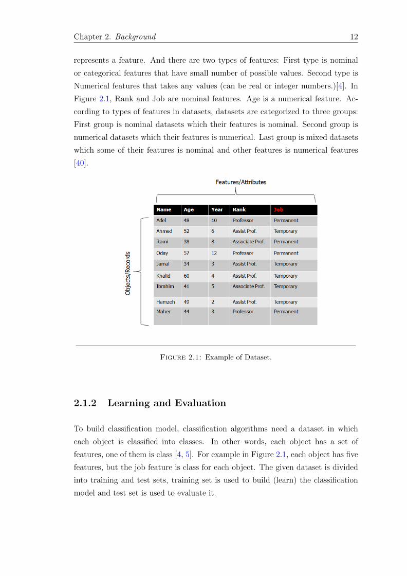
Chapter 2. Background 12
represents a feature. And there are two types of features: First type is nominal
or categorical features that have small number of possible values. Second type is
Numerical features that takes any values (can be real or integer numbers.)[4]. In
Figure 2.1, Rank and Job are nominal features. Age is a numerical feature. Ac-
cording to types of features in datasets, datasets are categorized to three groups:
First group is nominal datasets which their features is nominal. Second group is
numerical datasets which their features is numerical. Last group is mixed datasets
which some of their features is nominal and other features is numerical features
[40].
Figure 2.1: Example of Dataset.
2.1.2 Learning and Evaluation
To build classification model, classification algorithms need a dataset in which
each object is classified into classes. In other words, each object has a set of
features, one of them is class [4, 5]. For example in Figure 2.1, each object has five
features, but the job feature is class for each object. The given dataset is divided
into training and test sets, training set is used to build (learn) the classification
model and test set is used to evaluate it.

Chapter 2. Background 13
2.1.3 Classification Performance
Accuracy is one important measure that is used to evaluate the performance of
classification [4]. To calculate the classification accuracy, it is applied on test set,
then count the number of correct predictions and divide it by the total number of
predictions, multiply it by 100 to convert it into a percentage. But the accuracy
is not enough to evaluate the performance in some datasets, especially when most
objects are assigned to specific class. For this, we need another measures to eval-
uate a classification performance for each class in dataset in addition to accuracy
that evaluates the overall correctness of the classifier [43, 44].
Precision and Recall are very efficient to evaluate the classification model for each
class when the accuracy is high. Precision is a fraction of correct predictions for
specific class from the total number of predictions (Error + Correct) for the same
class. Recall (also known as sensitivity) is a fraction of correct predictions for
the specific class from the total number of objects that belong to the same class
[43, 44].
Most classification algorithms summarize the results in confusion matrix [45]. It
contains information about predicted and actual classifications. Table 2.1 shows
the confusion matrix for two classes (A and B), and the entries as follows.
Predicted
Class A Class B
Actual Class A TA FB
Class B FA TB
Table 2.1: Confusion Matrix.
TA: the number of correct predictions that an object is A.
FA: the number of incorrect of predictions that an object is A.
TB: the number of correct predictions that an object is B.
FB: the number of incorrect predictions that an object is B.
Accuracy(Overall) =TA+ TB
TA+ FB + FA+ TB(2.1)

Chapter 2. Background 14
Precision(A) =TA
TA+ FA(2.2)
Recall(A) =TA
TA+ FB(2.3)
2.1.4 Classification Algorithms
Many classification algorithms have been proposed to build the classification model.
Decision Tree and naıve Bayes two different types of classification algorithms that
are most common[3, 4, 46]. This section reviews briefly the decision tree and naıve
Bayes classification algorithms that will be used in this thesis to measure the clas-
sification performance, For more details about Decision Tree and naıve Bayes, you
can visit [46].
2.1.4.1 Decision Tree
Decision Tree (DT) is a method for approximating discrete valued functions [4]
and it summarizes training set in the form of a decision tree. Nodes in the tree
correspond to features, branches to their associated values, and leaves of the tree
correspond to classes. To classify a new instance, one simply examines the features
tested at the nodes of the tree and follows the branches corresponding to their
observed values in the instance. Upon reaching a leaf, the process terminates, and
the class at the leaf is assigned to the instance [3].
To build a DT from training data, DT’s algorithms use greedy approach to search
over features using a certain criterion such as gain and gini index to evaluate
the features in order to select the best feature for splitting the input training
set(objects) into smaller subsets to create a tree of rules. In more details, if the
subsets of objects belong to the same class, then the node is class label. But if the
subsets of objects belong to more than one class, then split it to smaller subsets.
Recursively apply these procedures to each subset until a stop criterion is met
[41, 46].

Chapter 2. Background 15
2.1.4.2 Naıve Bayes
Naıve Bayes (NB) is a simple probabilistic classification algorithm that uses Bayes
theorem with independent assumption between the features to predict class mem-
bership probabilities. It calculates the probability of unseen instance based on each
class, then it assigns this instance to the class with the highest probability. Learn-
ing with the NB is straightforward and involves simply estimating the probabilities
from the training set. NB is easy to construct and efficient for huge datasets, but it
is weak when applied on datasets that have many redundant features, this means,
NB is a good classification algorithm to evaluate the FS approaches over redundant
features [3, 42].
2.2 Feature Selection
FS studies how to select minimum subset of features from the original set while
keeping high accuracy in representing the original features in short computational
time [2, 3]. according to[3] FS is ” process that chooses an optimal subset of
features according to a certain criterion”. This section reviews some concepts that
is related to FS. The Following section reviews general FS steps, filter FS, and
wrapper FS.
2.2.1 General Feature Selection Steps
In general, FS algorithms (approaches) include five basic steps: Initial subset,
generation strategy, objective function, stopping criterion, and validation step
[3, 10]. See figure 2.2. Generation strategy starts from initial step to generate
new subset of features for objective function (evaluation step) to measure the
quality of it. Algorithm continues generating new candidate subsets of features
until stopping criterion is met. FS steps are discussed as follows.
Initialization: Any FS algorithm (approach) starts from initial subset or subsets
of features. There are three types of initial subset. First, empty subset. Second,
full subset. And the last is random subset [3, 10].
Search Strategy: is responsible to generate new candidate subset of features to
objective function. It starts from one of the initial subsets: Empty subset, features

Chapter 2. Background 16
Figure 2.2: General FS steps [8].
are added. Full subset, features are removed. Random subset, features are added,
or removed or created randomly. Complete, random and heuristic are types to
generate the next candidate subset of features [3, 10].
• Complete Search: Searches for all combinations of subsets of features. If the
number of features in search space is n, this means the number of subsets
of features is 2n. But this type of search is very expensive and sometimes is
impractical.
• Heuristic Search: Makes smart choices to select the near optimal subset
without searching in all combination of features. It is fast, but it does find
the optimal solution.
• Meta-heuristics Search: Like heuristic Search, but Meta-heuristics Search
has faster, and more efficient convergence compared to heuristic Search.
Objective Function: is responsible to determine the quality of subsets of fea-
tures. This function is very important in any FS algorithms, because it guides the
algorithm to find the optimal subset of features.
Stopping criterion: is responsible to stop the algorithm when the candidate of
subset features met the objective function (found the best solution), or the number
of iterations reached the maximum [10? ]

Chapter 2. Background 17
Validation: This step is not a part of FS algorithm to search for subset of features.
It is responsible to validate/evaluate the FS algorithm by validating the selected
subset of features on the test set [3]. The results are compared with previous
results to determine the performance of algorithm [3].
All steps are important for FS approaches, but the search strategy, and objective
function are two main factors for determining the efficiency of FS approaches.
2.2.2 Filter and Wrapper approaches
According to objective function, FS approaches are generally categorized into filter
and wrapper approaches. Filter approaches select the feature subset independently
from any classification algorithms, and the subset of features are evaluated using
certain criterion such as dependency degree [11], distance measure [8] and infor-
mation measure[12]. In this type, objective function is indicator for classification
performance. FOCUS [47], RELIEF[48], LVF[38], Greedy search[49] are filter FS
approaches. Also, [18–26] are filter FS approaches that combine NIAs with rough
set theory. These approaches will be reviewed in next chapter.
Wrapper approaches include classification algorithm as part of the objective func-
tion to evaluate the selected feature subsets. In other words, classification algo-
rithm performance used objective function to evaluate the subset of features [2, 3].
Sequential forward selection[50], Sequential backward selection[51], linear forward
selection[52], PSO[53], ACO[54] are wrapper FS approaches.
Wrapper approaches give high classification accuracy on a particular classification
algorithm, because it mixed between the classification algorithm and objective
function. But it is very expensive, because each evaluation includes a training
processes and testing processes of the classification algorithm[55]. While filter
approaches are much faster and more general than wrapper approaches [2, 3].
This thesis focuses on filter approaches.
2.3 Summary
This chapter presented some of the essential background concepts for FS and
classification, as a basis for the work in this thesis.

Chapter 2. Background 18
The next chapter reviews typical related works in filter FS.

Chapter 3
Literature Review
This chapter reviews related works in filter feature selection for classification. In
general, dimensionality reduction approaches can be categorized into feature ex-
traction (transformation) and FS [1]. Feature extraction approaches apply a trans-
formation to dataset to project it into a new feature space with lower dimension,
and they need to make mapping between the original feature space to a new feature
space [1, 56]. Principle Component Analysis (PCA)[57] and Canonical Correlation
Analysis (CCA)[58] are examples of feature extraction. Where as FS, which the
work of this thesis focuses on, selects a subset of features from the original dataset
without any transformation and mapping. FS approaches are divided into two
main groups: First, ranked approaches which failed to find the nearest optimal fea-
ture subset. Second, feature subset approaches which are divided to three groups:
Complete, heuristic, and meta-heuristics approaches. Meta-heuristics approaches
are capable of finding the nearest optimal feature subset in shortest computational
time. NIAs are a very efficient type of meta-heuristics for FS’s search strategy.
This thesis aims to develop a new filter FS based on NIA and RSTDD, for this,
we focus on filter FS approaches that use NIA in their search strategy and use
RSTDD in their objective function. Appendix D shows the map of classifications
of dimensionality reduction.
3.1 Introduction
In general, chapter two reviews the classification and FS, and it shows the im-
portance of FS for classification. A lot of work of FS has been developed from
19

Chapter 3. Literature Review 20
70’s , and most of these FS approaches try to achieve three goals: First is feature
reduction which means select the minimum number of features without significant
reduction of classification performance. Second is short computational time. And
the last to support different data characteristics, which means the FS is efficient
for nominal, mixed, and numerical datasets with different number of features,
different number of objects, different number of classes, and different areas [3].
FS approaches are categorized into two groups [59, 60]: First is ranked approaches
which depend on single feature evaluation to select the best feature subsets.
Ranked approaches measure the score (quality) of each feature, and then these
features are ranked according to their score to select the best subset. Relief is a
ranked approach [48]. The main problem in these approaches, is that the relevant
features cannot be evaluated independently from the other features, therefore the
subset of top ranked features, may include high number of irrelevant and redun-
dant features. While the combination of different ranked features may contain
low number of irrelevant and redundant features [59, 61–63]. This means, ranked
approaches are not capable to achieve the optimal feature reduction, but they are
cheap. To avoid this problem, many FS are implemented with feature subset eval-
uation instead of single feature evaluation, these approaches are a second group
which is a feature subset approaches. Also feature subset approaches are catego-
rized into three groups based on search strategy that used in these approaches to
complete, heuristic, and meta-heuristics approaches [60].
Complete approaches search for all possible feature subsets to find the optimal
feature subset, this means, the number of feature subsets needs to be generated
is 2n, where n is the number of features. These approaches achieve the feature
reduction, but they are very expensive (exponential time), practically impossible
[3, 60, 64]. Focus approach is example of complete approaches [47]. Heuristic Ap-
proaches try to find the best feature subset without searching in all possible feature
subsets to reduce the computational time compared to complete approaches. The
complexity time of heuristic is quadratic, but the complete is exponential [60, 64].
In general, heuristic approaches apply local changes to the current feature subset
to reach to best feature subset. The main drawbacks of heuristic approaches are
they do not guarantee the optimal feature subsets, and it stuck to the local op-
timal which mean the neighbor solutions is worse than the current solution, and
the current solution is worse than global optimum [3, 60]. Greedy Search [49] is
example of heuristic approaches which are like ranked approaches do not achieve
Chapter 3. Literature Review 21
the feature reduction. Recently, meta-heuristic approaches show more desirable
results compared to previous approaches.
FS is optimization problem which is the problem of finding the best solution from
all feasible solutions [6], meta-heuristics algorithms are very efficient for this type
of problems [13, 14]. Meta-heuristics algorithms represent a group of approxi-
mate techniques that aim to provide good solutions computed in a reasonable
time for solving optimization problems, but does not guarantee the optimality
of the obtained solutions [13, 14]. In general, meta-heuristics algorithms have
more efficient, and fast convergence compared to heuristic algorithms [14]. NIAs
are powerful type of meta-heuristics algorithms which improve the population of
solutions in each iteration, and they are developed based on characteristics of bio-
logical systems like ants, bee, swarm of birds to find the source of food, and cuckoo
reproduction, therefore some of NIAs can be called biology inspired[65, 66]. The
main idea in these systems, agents/particles corporate with each other by an indi-
rect communication medium to discover the food sources, or achieve some things
[25]. The advantages of NIAs: They may incorporate mechanisms to avoid getting
trapped in local optima. They can be easily implemented. Also these algorithms
are able to find best/optimal solution in a reasonable time due to efficient conver-
gence [13].
Recently, many of filter FS that combines NIAs with RSTDD are widely used
to develop their objective function such as [18–26], because RSTDD is efficient,
easy to implement, no need to any additional information about data, and cheap
compared to mutual information and entropy methods [30, 73]. Following sections
review nine filter FS that combine NIA with RSTDD [18–26], in addition to two
FS approaches that use NIA without RSTDD [31, 32]. To easy reviewing these
approaches, firstly, RSTDD is reviewed, then ten approaches are revived according
to the NIA which is used in them.
3.2 Rough Set Theory
RST was developed by Zdzislaw Pawlak in the early 1982s [15] as a mathemat-
ical tool that deals with classificatory analysis of data table(structured dataset).
RSTDD and positive region are two important issues in data analysis to dis-
cover the dependency between the feature subsets and class labels. Positive region

Chapter 3. Literature Review 22
(POSp(Q)) contain all objects that can be classified to classes of Q using infor-
mation in P. The RSTDD can be defined in equation 3.1 [17, 35, 67]. Appendix
A contain more details about RST.
γP (Q) =|posP (Q)||U |
(3.1)
Where |U | is the total number of objects, |posP (Q)| is the number of objects in a
positive region, and γP (Q) is the dependency between feature subset p and classes
Q.
In the literature there are two frequently used objective functions that use RSTDD
and balancing it with the number of selected features (size of feature subset).
Jensen et al.[19] proposed the first one (equation 3.2) as follows:
Objectivefunction(P ) = γP (Q) ∗ |C| − |P ||c|
(3.2)
Also Xiangyang Wang et al. [21] proposed a second multi objective objective
function(equation 3.3) as follows:
Objectivefunction(P ) = α ∗ γP (Q) + (1− α) ∗ |C| − |P ||C|
(3.3)
Where |C| is the total features, |P | is the number of selected features, Q is class,
and γP (Q) is the dependency degree between feature subset and class label Q,
α belong to [0,1] and it is a parameter to control the importance of dependency
degree and subset size. Normally, the value of α is 0.9 to give most importance to
the dependency than the size of subset[21].
RSTDD is an indicator for classification performance, it gives the same impor-
tance to all feature subsets that have the same dependency degree, and this is not
correct for all feature subsets for classification algorithm. In general, features that
have more frequent values and higher relevance are more desirable to classification
algorithms, it helps these algorithms to build a classification model in easier and
faster way, and better classification performance[33]. For these reasons, RSTDD
is efficient for nominal datasets that their features have roughly the small set of
values, but inefficient for mixed and numerical datasets that have some features

Chapter 3. Literature Review 23
with large and different number of frequent values, and low frequent values in
some other features [1]. RSTDD measures the dependency between the feature
subset and class labels without measuring the frequent values. Measuring the de-
pendency in nominal datasets is enough because their features have high frequent
values, but in mixed and numerical datasets, it is necessary to measure the fre-
quent values in addition to dependency, because there is a big difference in number
of frequent values between features in each dataset, and the number of frequent
values in most numerical features is very low which helps to increase the value of
dependency degree between the subset and class label regardless of the average of
frequent values in these subsets.
Finally, RSTDD is inefficient for mixed and numerical datasets, one goal of this
thesis is to develop new objective function based on RSTDD with improved effi-
ciency for nominal, mixed, and numerical datasets. This means approaches [18–26]
that use RSTDD in their objective function are inefficient for mixed and numerical
datasets.
Before reviewing approaches [18–26] according to the search strategy (NIAs), we
define NIAs’ search mechanisms which plays an important role in the effective-
ness of each NIA. Local, global, and hybrid search are mechanisms that are used
in NIAs to update the population of feature subsets to solve the FS [68]. Local
Search aims to find the best possible solution to a problem (Global Optimum) by
iteratively moving from current solution to better neighbor solution. But some-
times, current solution is better than all neighbors’ solutions, and it is worse than
global optimum. In this case, the local search suffers from local optimum problem
and stops searching. The advantage of local search is that it is relatively efficient
(fast), but it is affected by poor initial solutions, and it does not guarantee the
global convergence [14, 68]. Global Search searches for the candidate solution in
all the search space until it finds the best solution or reaches maximum iterations.
But it is slow [14, 68]. Hybrid Search aims to increase the convergence more
efficiency (to avoid be trapped in local optimum), and to guarantee the global
convergence as soon as possible by using global search to generate initial solutions
for local search [68].

Chapter 3. Literature Review 24
3.3 Ant Colony Optimization
Ant Colony Optimization (ACO) is a NIA presented by Dorigo et al in 1992 [69],
it simulates the behavior of real ants that use chemical material called pheromone
to find the shortest path between their nest and the food source. And when each
ant finds the food it returns to nest laying down a pheromone trail that evaporate
over time, then each ant follows the path that has large amount of pheromone[69].
ACO uses graph to represent the search space, features are represented as nodes,
and edges between the nodes determine the best next connected feature. Every
ant selects one node then uses a suitable method (Heuristic measures) and amount
of pheromone material on each connected edge to select the best connected node
to construct the population of candidate feature subsets [69].
We found three approaches in the literature for feature selection based on ACO
and RST. The first approach is Ant Colony Optimization based on Feature Se-
lection in Rough Set Theory (ACOFS)[20]. An efficient Ant Colony Optimization
approach to Attribute Reduction in rough Set theory (ACOAR)[18] is the sec-
ond approach. The last approach is Finding Rough Set Reducts with Ant Colony
Optimization(AntRSAR) [19].
The three approaches update the pheromone trails on each edge after constructing
each solution, but in ACOAR the pheromone values are limited between the upper
and lower trail limits to increase the efficiency of algorithm.
The heuristic measure in the AntRSAR approach uses entropy information, but
ACOFS and ACOAR use RSTDD which makes ACOFS and ACOAR cost less
compared to AntRSAR, because the entropy information is expensive compared
to RSTDD.
In general, ACO has some drawbacks. First, complex implementation and slow
convergence, because it uses graph to represent the search space [13, 14]. Complex
implementation and slow convergence means, these approaches that use ACO are
very expensive, and not suitable for large datasets (maximum size of datasets that
are used in experiments of these approaches is 69 features [18–20]).

Chapter 3. Literature Review 25
3.4 Particle Swarm Optimization
Particle swarm optimization (PSO) is a NIA developed by Kennedy and Eberhart
[70]. In nature, PSO simulates the movements of a flock of birds around food
sources, a flock of birds moving over an area where they can smell a hidden source
of food. The one who is closest to the food tweets loudly, and the other birds tweet
around in its direction. This means the birds closer to the target tweets louder.
This work continues until one of the birds find the food [70, 71].
PSO uses Particles as birds to search for the best solution in search space which are
represented in binary representation. The position of each particle is a possible
solution and the best solution is the closest position of particle to the target
(food). Particles move in the search space to search for the best solution by
updating the position of each particle based on the experience of its own and its
neighboring particles. Each particle has three vectors, first vector represents the
current position, second one for the velocity of particle, and the last one represents
the best previous position that is called personal best (pbest). But the algorithm
stores the best solution in all particles in a vector called global best solution
(gbest) [70]. [21–23] are filter FS approaches that use PSO to generate population
of candidate feature subsets.
We found three approaches in the literature for solving FS using PSO and RSTDD,
the first is Feature selection based on Rough Sets and Particle Swarm Optimization
(PSORSFS) [21], the second is An Attribute Reduction of Rough Set Based on
PSO (ARRSBP) [22], and the last is supervised hybrid feature selection based on
PSO and rough sets for medical diagnosis (SPSO-RR) [23].
Xiangyang Wang, et al (PSORSFS) [21] added limitation to the particle velocity to
avoid local optima, and move the particle to near global optimal solution. Because
high velocity moves the particle far away from global optimal, and low velocity
causes the local optimal.
Hongyuan Shen, et al ARRSBP [22] changed the values of weight parameter from
0.1 to 0.9 to balance between the pbest and gbest in generations.
H. Hannah Inbara, et al (SPSO-RR) [23] developed two algorithms for medical
datasets. First, it combines the PSO and quick reduct based on dependency
degree. And second algorithm combines the PSO and relative reduct based on
relative dependency.

Chapter 3. Literature Review 26
In general, PSO is easy to implement, and cheap. But it has weak convergence,
trapped into local optimum when it is applied on large datasets (maximum size
of datasets that used in experiments of these approaches is 57 features) [70, 71].
Also PSO is affected by the poor initial solutions [71].
3.5 Artificial Bee Colony
Artificail Bee Colony(ABC) algorithm is a NIA that is inspired by the natural
foraging behavior of honey bees. ABC is proposed by Karaboga [72]. In nature
the colony consist of three types of bees, employed bees, onlooker bees, and scout
bees. The foraging process starts by scout bees that move randomly to discover
the food sources. When the scout bees find the food sources, they return to their
hive and then start dancing (Waggle dance) to share their information about the
quality of food sources with onlooker bees, then depending on this information
more bees are recruited (employed bees) to the richness food source, but if any
bee finds the food source is poor, the bees call scout bees to discover randomly
new source food and so on [72, 73].
The position of a food source represents a possible solution using binary repre-
sentation, and the nectar amount of food source considered as the quality of the
solution. Each bee tries to find the best solution. ABC combines the global search
and local search to find the best solution [72, 73]. The ABC algorithm starts with
the n scout bees that select randomly population of candidate solutions as initial
solutions. Then, these solutions are evaluated, and it selects the candidate solu-
tions that have maximum quality for local search, and the remaining for global
search to construct new population of candidate solutions. Then the quality of
each solution in new population is evaluated, if the algorithm gets the best solution
then the algorithm stops, otherwise it continues searching until it finds the best
solution or arrives to maximum number of iterations [72, 73]. [24–26]are filter FS
approaches use ABC to generate population of candidate feature subsets.
We found three approaches in the literature for solving FS using ABC and RSTDD,
the first is a Novel Discrete Artificial Bee Colony Algorithm for Rough Set based
fetaure Selection(NDABC) [24], and second is a Novel Rough Set Reduct Algo-
rithm for Medical Domain Based on Bee Colony Optimization BeeRSAR [25], and

Chapter 3. Literature Review 27
the last is an Independent Rough Set Theory Approach Hyprid with Artificial Bee
Colony Algorithm for Dimensionality Reduction (BeeIQR) [26].
Yurong Hu, et al. [24] combined ABC and RSTDD to solve FS in an efficient
way. This approach changed one feature by either adding one feature or removing
one randomly in local search, a major weakness of this approach. And it uses a
random mechanism in global search.
Suguna,et al [25, 26] proposed two approaches that are similar in all things except
the initial population started from feature core(Start from set of features) , but
[26] started randomly. In local search, more than one feature is randomly changed
with some criteria, and random strategy is used in global search.
In general, ABC is a very efficient algorithm that solves the local optimal problem
by using hybrid search mechanism. But the local search in this algorithm causes
slow convergence [27]. Also these approaches[24–26] are not suitable for large
datasets (maximum size of datasets that used in experiments of these approaches
is 69 features[24–26]).
3.6 Cuckoo Search
Cuckoo Search (CS) is a new and powerful NIA algorithm that was developed
by Yang and Deb in 2009[14]. CS is a search algorithm inspired by the breeding
behavior of cuckoos and L’evy flight behavior of some birds and fruit flies which
is a special case of random walks [28, 31, 32, 74]. The reproduction strategy for
Cuckoo is aggressive. Cuckoos use the nests of other host birds to lay their eggs
in, and rely on these birds for hosting the egg. Sometimes the other host birds
discover these strange eggs and they either throw these strange eggs or leave their
nest and build a new one. Cuckoos lay eggs that look like the pattern and color
of the native eggs to reduce the probability of discovering them. If the egg of the
cuckoo hatches first, then the cuckoo chick destroys all eggs in the nest to get all
the food that is provided by its host bird [28, 75].
Algorithmically, each nest represents a solution, CS aims to replace the ”not so
good” solution (nest) with a new one that is better. CS uses local and global
search (Hybrid search) to update the population of solutions, local search update

Chapter 3. Literature Review 28
the solutions that have highest quality, and the rest of solutions are replaced with
new solutions randomly in global search.
Many optimization problems in different domains are solved in by CS to achieve
improved efficiency, table 3.1 is repeated here from [76] to show some of these
applications for convince. For further details and applications, see [77].
Binary Cuckoo Search for feature selection [31, 87], and Binary Cuckoo Optimiza-
tion Algorithm for Feature Selection in High-Dimensional Datasets(BCOA) [32]
are two approaches that use BCS. But the first approach is a wrapper approach,
and the second is a filter approach. To the best of our knowledge, [31, 32] are the
only two FS approaches that use BCS alone in their search strategy. The following
paragraphs explain these two approaches in details.
Binary representation: Search space is modeled as a binary n-bit string, where
n is the number of features [31, 32]. BCS represents each nest as a binary vector,
where each 1 corresponds to a selected feature and 0 otherwise. This means each
nest represents a candidate solution, and each egg represents a feature.
Initialization strategy: Generating an initial population of n nests randomly by
initializing each nest with a vector of binary value. Both [31, 32] use this strategy
which does not cover all search space ( see section 4.3 for more details).
Objective Function: [31] uses Optimum-Path Forest (OPF) classification al-
gorithm [88] in its objective function. But BCOA[32] uses mutual information
(expensive[19]) in its objective function. This step is replaced by a new objective
function to develop a new filter FS approach (MBCSFS) to improve the compu-
tational time.
Local And Global Search Switching: Existing approaches use threshold value
(Value of objective function =25%) to control the nests that are used in local
search and global search. Nests that have a quality more than 25% are used for
local search, and the remaining nests for global search. But the threshold in [32]
is not clearly specified.
Local Search: BCS updates each nest that has a quality more than the predefined
threshold using Levy Flights which is a main point of strength of CS. More details
on Levy Flights can be found in appendix B. Both [31, 32] use Levy Flights in
their local search.

Chapter 3. Literature Review 29
Authors Methods Task of CS/Application
Davar Giveki et.al[78] Modified Cuckoo SearchWith SVM
To optimize two parameters Cand γ for SVM/ Classification
Milos MADICet.al[79]
Cuckoo Search With Ar-tificial Neural Networks
Surface Roughness Optimiza-tion In CO2 Laser Cutting/Laser cutting AISI 304 stainlesssteel
Ivona et.al [80] Cuckoo Search Multilevel Image ThresholdingSelection/ Segmentation of im-ages
M. Prakash et.al [81] Cuckoo Search Optimizing Job Scheduling /Job Scheduling for Grid Com-puting
Koffka Khan et.al [82] Cuckoo Search WithNeural Network
Optimizing Neural NetworkWeights/ Compute Health andSafety risk index for employeesusing NSCS
Moe Moe Zaw et.al[83]
Cuckoo Search Document Clustering/ WebDocument Clustering: 7 sectorbenchmark data set
Akajit Saelim et.al[84]
Modified Cuckoo Search Optimizing Path/ To locatethe best possible server in dis-tributed systems
Rui Tang et.al [25] K-Means And CuckooSearch
Optimize K-Means/Clustering
Ehsan et.al [85] Improved CuckooSearch With Feed For-ward Neural Network
Optimize Network WeightsAnd Convergence Rate OfCuckoo Search/ Classificationof Iris and breast cancer datasets
Sean P. Walton [86] Modified Cuckoo Search Optimization Of Functions/Applied to aerodynamic shapeoptimization and mesh opti-mization
D. Rodrigues et.al[31, 87]
Binary Cuckoo Search Feature Selection/ Theft de-tection in power distributionsystems for two datasets com-mercial and industrial obtainedfrom a Brazilian electricalpower company
MahmoodMoghadasian et.al[32]
Binary Cuckoo Op-timization Algorithmfor Feature Selectionin High-DimensionalDatasets
Feature Selection/ Search forfeature subset on six medicaldatasets
Table 3.1: Applications of CS in different domains[76, 77].
Chapter 3. Literature Review 30
Global Search: [31] uses the same technique in initial strategy to replace the
nests that have quality less than the a predefined threshold (25%). But the [32]
use Levy Flights in its global search, this means [32] uses local search only to
update the population of solutions.
Stopping Criterion: The algorithm in this approach stops when the number
of iterations reaches the maximum predefined by the user. But the Stopping
Criterion in [32] is not clearly specified.
In their Evaluation:
[31] approach uses parameters as α =0.1, threshold =0.25, iteration=10, popula-
tion=30, and applies it on two small datasets obtained from a Brazilian electrical
power company. This approach has been compared with some NIAs such as: bi-
nary particle swarm optimization and Binary firefly algorithm [89]. Results show
that BCS is efficient for FS, and it achieved the maximum accuracy or the same
classifier accuracy as other algorithms. But BCS has been found the fastest.
[32] approach uses parameters as α =0.5 to 0.9, maximum number of itera-
tion=1000, and applies it on six numerical and medical datasets. K-Nearest
Neighbor (KNN) classification algorithm is selected to measure the classification
accuracy. Results show the BCOA achieves better feature reduction compared to
other approaches that are used in its evaluation, but its evaluation is not clearly
specified, such as the approaches that are used in comparisons.
In general, CS algorithm[28] is a new and powerful NIA, and it uses hybrid mecha-
nism search to find the optimal solution, while its local search is very efficient, not
trapped in local optimal, and its implementation is simple. Unfortunately, [31] is a
wrapper FS, and its BCS is inefficient for datasets that have more than 20 features
and the number of features in optimal features subset is less than 25% from total
features(Section 4.3 explains why). [32] is a filter approach that uses expensive
objective function(mutual information is expensive[19]), and it uses local search
without global search, this means the search mechanism of search algorithm that
is used in [32] is not hybrid mechanism, while the main efficient point for CS is
the hybrid mechanism[28].

Chapter 3. Literature Review 31
3.7 Comparison
This section shows the general comparison between ACO, PSO, ABC, and BCS for
FS. ACO is very complex compared to PSO, ABC, CS, because it uses graph repre-
sentation compared to other that use binary representation, and ACO needs more
parameters than other. This makes the ACO most expensive. PSO, ABC, and
BCS use binary representation which makes the implementation of them mostly
cheap. The convergence of ABC and BCS is more efficient compared to ACO
and PSO, because the ABC and CS use hybrid search mechanism. But the CS
has more efficient convergence compared to ABC which its local search is very
weak compared to CS that use least number of parameters compared to other.
This mean, CS has fastest, most efficient convergence, easiest implementation,
and needs less parameters compared to other, and according to my knowledge, No
filter FS that use BCS is available.
Unfortunately, approaches [18–26, 31] that are reviewed in this chapter are not
efficient for datasets which have more than 70 features in best case (the number of
features is determined according to experiments of [18–26]) . Also they [18–26] are
not efficient for mixed and numerical datasets because they use RSTDD in their
objective function. Also BCS approach[31] is expensive because it is a wrapper
approach. But there is a potential to improve the BCS that is used in them to
become more efficient and fast by developing new filter FS.
3.8 Summary
This chapter reviewed the related works for filter Feature Selection(FS), and it
focuses on filter FS that combines the RSTDD and NIA.
Ranked and feature subset are types of FS approaches, ranked approaches are
cheap, but they failed to achieve the feature reduction. In feature subset FS ,
there are three types: Complete approaches that achieve feature reduction, but
they are very expensive. Heuristic approaches are cheap but they do not achieve
feature reduction. Recently, meta-heuristics approaches are cheap and mostly
achieve feature reduction.
NIAs are efficient type of meta-heuristics algorithms, ACO, PSO, ABC are NIAs
that are used in many filter FS approaches. ACO approaches are very expensive

Chapter 3. Literature Review 32
and complex, PSO and ABC are cheap and easy to implement compared to ACO,
but ABC has more efficient convergence than PSO, because ABC uses hybrid
search mechanism to update the population of solutions, but the main drawbacks
of ABC its that it is weak local search. For this, many researchers use CS to solve
many optimization problems in several domains, because the CS use hybrid search
mechanism, and its local search is very strong. BCS is binary model of CS, and it
is used to solve FS.
BCS that is used in approach[31] has some of drawbacks, such as its inefficient for
datasets that have more than 20 features. But the performance of BCS can be
improved to increase the efficiency and speed of convergence.
The main limitation of the approaches are reviewed, first, they are efficient for
datasets that have less or equal 70 features in best case, and most of them that
used RSTDD in their objective function are inefficient for mixed and numerical
datasets.
Next chapter presents the proposed algorithm .

Chapter 4
Proposed Algorithm
This chapter proposes a new classification filter feature selection approach that
is called Modified Binary Cuckoo Search based on rough set theory for Feature
Selection (MBCSFS). MBCSFS improves the binary cuckoo search by developing
new initialization, global updating, and local updating, switching and termina-
tion mechanisms. Also MBCSFS develops new objective function to measure the
dependency between the combination of features and class labels using RSTDD,
and it measures the average number of distinct values of feature subsets. MBCSFS
aims to find the minimum feature subset without significant reduction in classifica-
tion performance with in best achievable computational time for nominal, mixed,
and numerical datasets with different sizes.
4.1 Introduction
FS for classification aims to minimize the number of features and maximize the
classification performance, for this FS is called multi objective problem [90]. Two
main factors are needed to develop filter FS approach. The first is a search strategy
to search in the search space for a candidate feature subsets, and the second is an
objective function responsible to evaluate these candidate feature subsets to find
the best subset that has less number of features, highest relevancy to class labels,
and highest frequent values . NIAs are generally efficient for searching [66], CS is
a new and a powerful NIA [28], and BCS is a binary version of the CS [31, 32].
33

Chapter 4. Proposed Algorithm 34
In the literature, filter FS approaches especially that combine NIAs and use
RSTDD failed to perfrom well in many datasets, that are mixed and numerical
datasets, and datasets that have more than 76 features [18–26]. BCS algorithm
used in [31] is a good search algorithm for datasets which have less than 20 fea-
tures, see section 4.3 . But there is a potential to improve the convergence of BCS
algorithm to become faster, and more efficient for datasets that have more than
20 features (experiments in chapter 5 prove modified BCS is more efficient up to
617 features).
MBCSFS is a new classification filter FS approach that has the following contri-
butions:
• According to my knowledge, MBCSFS is the first classification filter FS
approach that uses BCS and RSTDD.
• Developed a new objective function that uses RSTDD and number of dis-
tinct values to achieve improved efficiency for nominal, mixed, and numerical
datasets.
• Improving the BCS
– New initialization and new global search mechanisms to speed the con-
vergence, and guarantee the global convergence.
– New local search to decrease the number of iterations needed to find the
global optimal solution, and to increase the chance to find this solution.
– New switching mechanism: guarantee the local and global search in
each iteration to increase the efficiency of convergence.
– New termination mechanism to achieve improved computational time
over the baseline BCSFS.
The pseudo code of Basic BCS with the traditional objective function [19](BCSFS)
is shown in algorithm 4.1. The main difference between the existing approach that
used BCS [31] and the algorithm 4.1, is the objective function shown in step 3.1
in this algorithm. BCSFS is described as the baseline to test the performance of
the newly proposed algorithms (MBCSFS).
The remainder of this chapter is organized as follows. The second section presents
the new objective function. The third section describes the new initialization

Chapter 4. Proposed Algorithm 35
Input:
Trainingset
Number of nests n.
Value of Pa .// To control of local and global search
Number of maximum iteration T.
Output: optimal feature subset g_best.
Step 1: Initialize the population of solutions by random method.
Step 2: t=1.
Step 3: Repeat
Step 3.1: Evaluate the population (n nests/ solutions) by equation (3.2)
Step 3.2: Sort the population of candidate solutions descending
according to objective function.
Step 3.3: if g_best< first solution, then g_best=first solution
Step 3.4: (Global Search) Select the worst nests (solutions) which their quality are
less than Pa (0.25) and replace them to new solutions randomly.
Step 3.5: (Local Search) Select the best nests (remaining nests/solutions),
and update them using L´evy flights.
Step 4: t=t+1.
Step 5: Until (t > T).
Step 6: Output g_best.
Algorithm 4.1: Pseudo Code of Basic BCS with traditional Objective func-tion [19] (BCSFS).
mechanism. New updating mechanisms are presented in the fourth section. New
stopping criterion mechanism is described in fifth section. The sixth section pro-
vides summary of this chapter.
4.2 New Objective Function
In general, feature subset that has high relevancy to class labels, and high frequent
values in its features, helps to increase the classification performance in many
classification algorithms [33]. High frequent values means the chance to repeat
these values which are used to build classification model in future is high, but the
high frequent values alone is not enough to give a good indicator for classification

Chapter 4. Proposed Algorithm 36
performance, because the dependency between the feature subset and class label
may be low. RSTDD is good theory to measure the dependency between the
feature subset and class labels, but it is not enough alone as a good indicator
for classification performance in all datasets especially datasets that have low and
different frequent values(Mixed and numerical datasets).
Objective functions [19, 27] that use RSTDD are good when they are applied on
nominal datasets, or the datasets which have the same number of frequent values.
But RSTDD is not efficient when applied on mixed and numerical datasets which
their features have number of different frequent values.
Therefore it is necessary to develop a new efficient objective function that is capa-
ble to evaluate the feature subset by balancing between three objectives (frequent
values, dependency degree, and number of selected features). We give Three Ob-
jectives and Global (3OG) name for this objective function. We develop 3OG
objective function in the following sections:
4.2.1 Frequent values
Feature has high frequent values, means the number of distinct values in this
feature is low. We use the number of distinct values and total number of objects
to calculate the percentage of distinct values in each feature, and this is indicator
for frequent values, see equation 4.1. This equation gives low percentage when the
frequent values is high. For example, ZOO dataset [40] has 100 objects, its animal
name feature has 100 values, and eggs feature has two values. Eggs feature has high
frequent values, equation 4.1 gives 2% as a percentage of distinct values for eggs
feature. But the frequent values of animal name feature is very low (no frequent
values), and the result of equation 4.1 for animal name feature is 1. Remember
the relationship between the frequent values and equation 4.1 is inverse.
Distinct%(R) =|Distinct values(R)|
|Objects|(4.1)
Where R is a subset of features, distinct values(R) is the average of number of
distinct values for R features, and objects is the number of total objects in dataset.

Chapter 4. Proposed Algorithm 37
4.2.2 Dependency Degree
We use RSTDD (equation 3.1) to measure the dependency between the feature
subset and class labels.
4.2.3 Balancing between the Percentage of Distinct Values
and Dependency Degree
In general, high dependency degree is a good indicator for relevancy between the
feature subset and class label. Low distinct percentage for feature subset is a
good indicator for high frequent values. In other words, feature subset which has
maximum dependency degree and minimum unique values percentage is desirable
for classification algorithms [33]. This means, the dependency degree is close to
one (100%) and percentage of unique values is close to zero. We develop equation
4.2 to balance between them.
Quality%(R) = DependencyDegree%(R)− UniqueV alues%(R) (4.2)
Equation 4.2 gives high quality when the feature subset is more desirable for clas-
sification algorithms. For example, in Zoo dataset, assume there are two feature
subsets. First subset is {Animal name, aquatic, domestic}, and distinct % for
it is 34%, and dependency degree is 100%Second subset is {hair, milk, predator,
backbone, venomous} and average of distinct % for it is 2%, and dependency
degree is 96%. As dependency degree, first subset is the best, because it has
higher dependency degree compared to second. But when we measure the classifi-
cation accuracy of both subsets using decision tree J48 in Weka, the accuracy for
first subset is 43%, and 93% for second subset. This means the second subset is
better than first subset, because the second subset has high frequent values and
high dependency degree. Dependency degree (first subset) gives bad indicator
for classification algorithm (Decision tree J48), because it has low frequent values
compared to second subset.
When applying our equation 4.2 for both subsets, quality (first subset) is 100%
- 34%=66%, but the quality (second subset) =96%-2%=94%. As equation 4.2,
second subset achieves better classification accuracy compared to the first subset.

Chapter 4. Proposed Algorithm 38
4.2.4 Balancing Between the Quality and Number of Se-
lected Features
FS is multi objective problem, maximum classification performance, and minimum
number of selected features are objectives of FS. Equation 4.2 achieves the first
objective only, now we modify this equation to achieve two objectives, see equation
4.3.
Quality(R) = Equation4.2 ∗ |C| − |R||C|
(4.3)
Where C is the number of available features, R is the number of selected features.
The idea of this balancing is taken from equation 3.2.
Following sections explain how the BCS is improved to achieve faster global con-
vergence.
4.3 New Initialization Mechanisms
In BCS [31], in its initialization strategy, each solution (or nest) is randomly ini-
tialized, as shown in pseudo code 4.1. Given its binary selection, from a search
space, the probability of every feature belonging successfully to the selected fea-
tures category for search has a 50% chance of being selected [60]. The aim is to
maximize the number of different features, to cover a wide range from across the
search space, that are selected for each solution search. A good initialization strat-
egy is, thus, one capable of generating initial nests with as many different number
of features across the full range as possible, such that the selected features for the
search space cover most of the possible numbers of selected features. For example,
assume the total number of features in a search space is 50, this means, the possi-
ble number of features to select for the search ideally should be from any of 0 to
50. A good initialization strategy is one that allows selecting most of the possible
numbers of selected features from across the range from 0 to 50, not one that just
perhaps centers its selection of features from around 20-30 of the search space for
example.
However, the pseudo code in 4.1 does not guarantee to generate the most pos-
sible numbers of selected features, to cover a wide range, from across the search

Chapter 4. Proposed Algorithm 39
space. To understand the reason behind that, let’s discuss the probability theory
of this pseudo code (Traditional initialization strategy). The number of successes
in a sequence of n (total number of features) independent selected or not selected
experiments is the binomial distribution [60], with each success has probability p
(50%), and the n (in our case is the total number of features) play a main role in
determining the probability of numbers of successes(selected features). The prob-
ability of getting exactly k successes in n trials is given by the probability mass
function. Figure 4.1 shows some examples of the probability mass function, first
example ( n=9 features) shows the initial strategy has a good chance to cover most
possible numbers of selected features. But in the second example(n=20 features)
show the probability of generating feature subsets that have less than four features
or more than 16 features is close to zero. While the third example(n=33) shows the
probability of generating feature subsets that have less than 10 features or more
than 25 features is close to zero. And in the last example(n=90 features), feature
subsets which have less than 30 features or more than 60 features have probability
close to zero to select in the initial strategy. In general, Binomial distribution
shows the probability is very small to select the feature subsets with a number of
features less than 25% or more than 75% of total number of features that is more
than 20. In other words, this initialization strategy misses the small and large
optimal feature subsets. Also the experiments in chapter 5 shows similar results,
table 5.4 in chapter 5 shows the smallest feature subset that can be selected via
this initialization strategy with different number of features.
For nest=1 to population size do
For egg=0 to totalFeatures-1 do
Solution [nest] [egg] =random (0, 1) // 1 means selected, 0 means removed
Pseudo code 4.1: Initialization Mechanism for BCSFS .
This strategy does not help the BCS to cover most the the search space (cover most
of the possible numbers of selected features), and this causes weak convergence. To
investigate the initialization strategy in BCS for FS, new mechanism that divides
the initialization strategy to three parts is proposed to increase the efficiency of
convergence and speed of BCS. In other words, the main goal of the splitting is
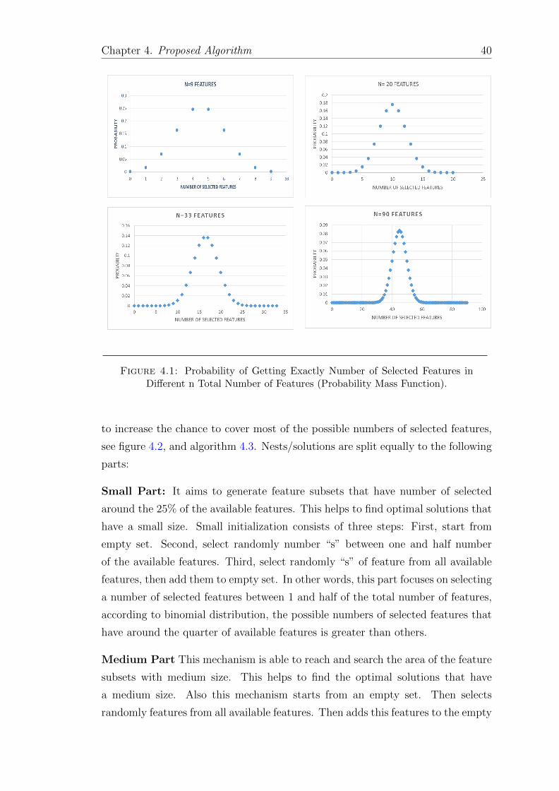
Chapter 4. Proposed Algorithm 40
Figure 4.1: Probability of Getting Exactly Number of Selected Features inDifferent n Total Number of Features (Probability Mass Function).
to increase the chance to cover most of the possible numbers of selected features,
see figure 4.2, and algorithm 4.3. Nests/solutions are split equally to the following
parts:
Small Part: It aims to generate feature subsets that have number of selected
around the 25% of the available features. This helps to find optimal solutions that
have a small size. Small initialization consists of three steps: First, start from
empty set. Second, select randomly number “s” between one and half number
of the available features. Third, select randomly “s” of feature from all available
features, then add them to empty set. In other words, this part focuses on selecting
a number of selected features between 1 and half of the total number of features,
according to binomial distribution, the possible numbers of selected features that
have around the quarter of available features is greater than others.
Medium Part This mechanism is able to reach and search the area of the feature
subsets with medium size. This helps to find the optimal solutions that have
a medium size. Also this mechanism starts from an empty set. Then selects
randomly features from all available features. Then adds this features to the empty

Chapter 4. Proposed Algorithm 41
Figure 4.2: Probability Mass Function of New Initialization Mechanism.
set. We see this initialization focuses on the feature subsets that have around half
number of available features. This part is same as the traditional initialization
strategy, see figure 4.1 that shows the possible numbers of selected features that
have around the half number of available features is greater than others.
Large Part: This mechanism is capable of searching for the feature subsets that
are selected close to the number of available features. This helps to find the
optimal solutions that have around 75% of number of available features. Large
initialization consists of three steps: First, Start from full set. Second, select
random number “s” between the one and half the number of available features,
then select randomly ”s”’ features. Third, remove these features from full set.
4.4 New Updating Mechanisms
In general, local and global search are two mechanisms that are used to update
the population of solutions. Local search aims to improve the current solutions by
applying small modifications to them in the hope of finding a better one (global
optimal) in shorter computation time. But this mechanism (local search) may be
unable to prove global optimality, because the initial solutions affect it. Global
search does not depend on the initial solutions to find the global optimal, but it
needs a large number of iterations to find the global optimal if possible. Many

Chapter 4. Proposed Algorithm 42
algorithms combine local and global search in a new mechanism to avoid the
disadvantages of them [28, 72]. Global search is used to generate new candidate
solutions that are used by the local search to find global or nearest optimal solution.
CS is one of these algorithms, and it has very efficient local search mechanism
compared to other algorithms. BCS [31] as CS is efficient, but there is a potential to
improve the local and global search to BCS to become faster, and guarantee global
convergence. Following sections explain how to improve the updating mechanisms.
4.4.1 New Global Search
The main key of global search is to cover all search space as much as possible to
guarantee the global convergence, and increases the speed of it. But the global
search in BCS and some other approaches does not achieve this key when the
search space has more than 20 features, because it uses the same strategy that is
used in the initial strategy. Therefore it’s necessary to modify BCS’s global search
to as much of the search space as possible. As a new initialization mechanism,
the global search divides the searching into three parts: First part is small search
that focuses on feature subsets which size is around the 25% of available features.
Second part is medium search that is interested in the subsets which size is around
half number of the available features. Last part is large search that focuses on the
subsets which size is around the 75% from available features, see algorithm 4.3.
4.4.2 New Local Search
Local search applies small modifications to improve the current solutions to find
the local optimal solutions that hopefully lead to global optimal or nearest of it.
Remember, the goal of local search is speeding up the convergence to get the global
optimal solution in less number of iterations. BCS uses levy flight to move from
the current solution to a new one. Step size α in levy flight is main factor in local
search. The higher value of α means increasing the size of the modifications. The
value of α in BCS is fixed (Typically is 0.25), this means the modification is large
and same size in all iterations. Initially we need a large modification to increase
the diversity of feature subset, but if this size stays large, this causes going far away
from global optimal solution. To improve the local search, according to [85] our
approach modifies the value of α to become variable instead of being fixed. In the

Chapter 4. Proposed Algorithm 43
early generations, the size of modifications must be large enough to increase the
diversity of feature subsets, then the size of modifications must be decreased in the
following iterations to avoid going far from the optimal solutions (and reducing
the number of iterations) is needed to get the optimal subsets. Therefore, the
value of α decreases as the number of iterations increases.
4.4.3 Global versus local Ratio (New Switching Mecha-
nism)
BCS uses the probability P to control the nests for local and global search, Nests
that have quality (result of objective function) less than P are updated by global
search, and remaining nests are updated by local search. But there is a problem
in this mechanism. Assume the quality of all nests is more than P or less than P
in some iteration, this means, BCS become local or global search instead of hybrid
search. Please note, a hybrid search mechanism helps to increase the efficiency of
convergence. We develop a new switching mechanism that guarantees the local
and global search are run in each iteration to increase the chance to find the best
feature subset in a lesser number of iterations. New switching mechanism divides
the population into two parts: first part has the nests that have the highest quality
for local search, and the second part has the remaining nests for global search. The
ratio of these parts is determined by user.
4.5 New Stopping Criterion
It is very difficult to determine if the algorithm finds the optimal feature subset
or not, because the evaluation of feature subset depends on its size and quality.
For this reason, most existing approaches uses maximum iterations to stop the
algorithm. In most cases, this causes wasting much time without improving the
solutions. For example, maximum iteration is 20, third iteration finds the best
feature subset, and algorithm continues searching until it reaches maximum iter-
ations without improvement over the feature subset that was found in the third
iteration. This means, the time of seventeen iterations is wasted without any use.
Therefore, a new stopping criterion is proposed to stop the algorithm before reach-
ing maximum iterations, which is to stop if there was no chance to improve the

Chapter 4. Proposed Algorithm 44
best feature subset. The idea of this criterion is when in a number of successive
iterations(determined by user) there is no improvement in the best feature subset,
the algorithm stops. See algorithm 4.3.
Parameters in algorithm 4.3 has the same values as those used in our experiments.
Input:
Trainingset
Number of nests n.
Number of maximum iteration T.
Number of successive iteration stopCriterion.
Local versus global ratio ratio.
Total number of features features
Output: optimal feature subset g_best.
Step 1: Divide equally the population of n nests into three parts to initialize them.
Step 1.1(Small part): Initialize each nest in this part by selecting randomly number of
Features around the quarter of features.
Step 1.2(Medium part): Initialize each nest in this part by selecting randomly number of
Features around the half of features.
Step 1.3(Large part): Initialize each nest in this part by selecting randomly number of
features around the Three quarters of features.
Step2: While (t<T or stop Criterion) do
Step 2.1: Evaluate each nest using 3OG objective function.
Step2.2: Sort the nests descending according to the value of 3OG.
Step 2.3: if (g_best< first nest)
g_best=first nest
Step2.4: Divide the population of n nests according the predefined ratio
into best nests and worst nests parts.
Step2.4.1 (local search): Update the best nests using levy flight.
Step 2.4.2(Global search): Update the worst nests as Step 1.
Step2.5: t=t+1.
Step 3: Print g_best.
Algorithm 4.3: Pseudo Code of Modified Binary Cuckoo Search based onRough Set Theory for Feature Selection(MBCSFS).

Chapter 4. Proposed Algorithm 45
4.6 Summary
The goal of this chapter is developing a new filter BCS for FS to improve the
performance of the basic BCS, which is expected to achieve feature reduction in
short computational time for different datasets with different characteristic (sizes,
types, classes). To achieve that goal, all main parts in BCS were modified to
speed up the convergence, guarantee the global convergence, and achieve efficient
evaluation for feature subsets.
New objective function based on RSTDD and distinct values was developed to
guide the MBCSFS to feature subsets that have minimum number of features
with maximum classification performance. This objective function calculates the
quality of feature subsets by balancing between the relevancy, frequent values
and their size. The function used RSTDD to measure the relevancy between the
selected features and class labels. And it used distinct values to measure the
frequent values of feature subsets.
This chapter shows the new initialization and new global search mechanisms.
MBCSFS divides the initialization and global search to three parts to make it
suitable for different sizes of datasets and guarantee the global convergence. First
part is for small optimal solution. Second part is for medium size. And the last
part is for large size of optimal solutions.
Also this chapter shows the modification of local search mechanism that aims to
increase the chance to find the global optimal solution in less number of iterations.
The main idea is that the size of modifications of the current solutions is decreasing
when the number of generations/iterations is increased.
New stopping criterion is proposed in this chapter to stop the algorithm when in
three successive iterations there is no improvement in the current solution. This
helps to avoid wasting time without any use.
Next chapter shows the design of the MBCSFS and experiments to evaluate it
(MBCSFS), and compares it to baseline, particle swarm optimization, and genetic
algorithms approaches.

Chapter 5
Evaluation and Results
In order to evaluate the performance of MBCSFS, thesis takes an empirical ap-
proach by comparing it to three filter FS approaches after applying them on 16
datasets.Thesis selects filter FS approaches in evaluation, because MBCSFS is a
filter approach.
This chapter aims to show the datasets and the methodology evaluation used
in the experiments, also it discusses the results of MBCSFS compared to base-
line(BCSFS), Genetic[37] with Correlation based on Feature Selection(CFS)[38],
and PSO[39] with CFS approaches.
5.1 Evaluation Methodology
This section describes the methodology we detected to evaluate our work.
5.1.1 Datasets selection
In order to evaluate the performance of MBCSFS, a group of experiments have
been run on sixteen datasets, where these datasets are taken from the University
of California at Irvine, known as the UCI data repository of machine learning
database [40]. UCI classifies datasets for classification according to types of their
features to three groups: First is nominal or categorical group which contains
28 datasets. Numerical or continuous is the second group which contains 137
46

Chapter 5. Experimental Design and Evaluation 47
datasets, and the last is mixed group which has 37 datasets. These feature types
are illustrated in chapter 2.
Our approach aims to achieve feature reduction for nominal, mixed, and numerical
datasets with different characteristics especially different number of features in
addition to different number of objects and different number of classes. To evaluate
this, sixteen datasets that posses these characteristics are selected randomly as
follows: Four datasets from nominal group, four datasets from mixed group, and
eight datasets from numerical group. Table 5.1 shows these datasets and their
characteristics, each dataset is made available as a text file of a CSV format.
# Dataset Features Objects Class
Values.
Domain
(Area)
Nominal Datasets
1 Congressional Voting Records 16 435 26 Social
2 Mushroom 22 8124 2 Life
3 Soybean(small) 35 386 19 Life
4 Lung Cancer 56 32 3 Life
Mixed Datasets
5 Zoo 17 101 7 Life
6 Hepatitis 19 155 2 Life
7 German Credit Data 20 1000 2 Financial
8 Dermatology 33 366 6 Life
Numerical Datasets
9 Breast Cancer Wisconsin (Original) 9 699 2 Life
10 Wine 13 178 3 Physical
11 Segment 19 1500 7 Computer
12 Spectf 44 80 2 Life
13 Connectionist Bench (Sonar) 60 208 2 Physical
14 Libras Movement 90 360 15 N/A
15 Musk (Version 1) 168 476 2 Physical
16 ISOLET-test 617 1559 26 Computer
Table 5.1: Datasets.
The following is a brief description of the datasets.
Congressional Voting Records. This dataset includes votes for each of the
U.S. houses of representatives’ congressmen on the 16 key votes identified by the
Congressional Quarterly Almanac (CQA). There are 16 nominal features in this
dataset, and each one has two distinct values. 435 objects are classified into two
classes, 168 objects for the first class, 267 objects for second class.
Mushroom. It contains records drawn from the audubon society field guide to
north American mushrooms. This dataset has 22 nominal features with different

Chapter 5. Experimental Design and Evaluation 48
number of distinct values( from 2 to 12). Also it has 8124 objects that are classified
roughly to two classes.
Soybean(small). The task is to diagnose diseases in soybean plants. It has 35
nominal features that have from 1 to 7 distinct values. There are 47 objects which
are classified to 4 classes, one class has 17 objects and each class in remaining
classes has 10 objects.
Lung Cancer. It has 55 nominal features with 2 to 4 distinct values. There are
32 objects, 9 objects for first class, 23 objects for second class.
Zoo. It has 17 features (16 nominal features, 1 numerical feature). Most of
nominal features have two distinct values, but the numerical feature has 6 distinct
values. 101 objects are classified into seven classes, 41 objects for mammal class, 20
objects for bird class, 5 objects for reptile class, 13 objects for fish class, 4 objects
for amphibian class, 8 objects for insect class, and 10 objects for invertebrate class.
Hepatitis. It has 19 features, 7 numerical features which have from 30 to 85
distinct values, and 12 nominal features which have 2 distinct values. This dataset
has 155 objects, 32 objects belong to one class, and remaining objects belong to
second class.
German Credit Data. It has 7 numerical features which have 3 to 921 distinct
values, and 13 nominal features which have from 2 to 10 distinct values. 1001
objects are classified into two classes, 701 objects for good class, 300 objects for
bad class.
Dermatology. This dataset has 34 features, one feature is numerical which has
60 number of distinct values, and 33 nominal features which have distinct values
from 2 to 4. 366 objects are classified into six classes, 61 objects for first class,
112 objects for second class, 72 objects for third class, 52 for fourth class, 49 for
fifth class, and 20 objects for sixth class.
Breast Cancer Wisconsin. It is obtained from the university of wisconsin
hospitals, it has 9 numerical features, each one has ten distinct values. There are
699 objects, 458 objects classified into benign class, and the remaining objects are
classified into malignant class.
Wine. The data of this dataset are the results of a chemical analysis of wines
grown in the same region in Italy. It has 13 numerical features with different

Chapter 5. Experimental Design and Evaluation 49
number of distinct values (from 39 to 133 unique values). There are 178 objects
in this dataset, 59 objects are classified into first class, 71 to second class, and 48
objects are classified into third class.
Segment. This dataset describes diagnosing of cardiac Single Proton Emission
Computed Tomography (SPECT) images. It has 44 numerical features with dif-
ferent number of unique values (from 21 to 36 distinct values). Also it has 80
objects which are classified equally into two classes.
SPECTf. This dataset describes diagnosing of cardiac Single Proton Emission
Computed Tomography (SPECT) images. It has 44 numerical features with dif-
ferent number of distinct values (from 21 to 36 distinct values). Also it has 80
objects which are classified equally into two classes.
Connectionist Bench (Sonar). It has 60 numerical features with different num-
ber of distinct values(from 109 to 208). Also it has 208 objects roughly classified
into two classes.
Libras Movement. It has 90 numerical features, and they have number of unique
values from 172 to 235. There are 360 objects classified equally into 15 classes.
Musk (Version 1). This dataset describes a set of 92 molecules of which 47
are judged by human experts to be musks and the remaining 45 molecules are
judged to be non-musks. The goal is to learn to predict whether new molecules
will be musks or non-musks. This dataset has 168 numerical features with different
number of distinct values(from 32 to 476). And it has 476 objects are classified
into two classes. 207 objects for first class, 269 for second class.
ISOLET-test. This dataset has 617 numerical features with different number of
distinct values (from 2 to 1420). Also it has 1559 objects are classified equally to
26 classes.
5.1.2 Evaluation method
To evaluate how effective FS is to a classification algorithms, two general evaluation
approaches are commonly employed: direct and indirect [3]. The direct approach
is used when the certain relevant features of a dataset are already known, and an
algorithm is directly evaluated for FS against them. However, often we do not

Chapter 5. Experimental Design and Evaluation 50
have a prior knowledge of the relevant features about the datasets. Hence, most
FS approaches use the indirect approach which does not need any prior knowledge
about datasets. Indirect approach uses classification algorithms to measure the
classification performance (in item of accuracy, Precision, and recall) for selected
features [3, 18–26].
Two main comparisons are commonly used in the indirect approach to evaluate
the FS. First, before and after comparison which measures the classification per-
formance of all available features and for selected features. Second comparison,
checks the efficiency of a specific FS approach by comparing it to other FS ap-
proaches. Number of selected features or size reduction (size reduction is the
percentage between the number of removed features and all available features),
classification performance, and computational time are three factors that may be
used in this comparison. To examine whether FS is proper for different classifi-
cation algorithms, at least two different types of classification algorithms need to
be used to measure the classification performance. NB and DT are common algo-
rithms that are used to evaluate FS , they efficient and easy to construct [3]. More
details for these classification algorithms were provided in chapter 2 [3, 63, 91].
Given that we do not have prior knowledge of the datasets, the indirect evaluation
approach is appropriate for our case. We will employ the indirect evaluation com-
bined with ”before and after” comparison to compare our developed approach/al-
gorithm(MBCSFS) with the baseline approach(BCSFS). In addition, it will be
compared to genetic [37] with CFS [38] and PSO [39] with CFS [38]. Different two
classification types (DT [41] and NB [42]) are used to measure the classification
performance for all approaches that are used in the experiments. Classification
performance means in this thesis, accuracy, precision, and recall classification mea-
surements, see section 2.1.3.
5.1.3 Benchmarking and Experiment Design
All implementations are run on a personal computer running Windows 7 with (i5)
2.4 GHZ processor and 6GB memory. MBCSFS and BCSFS are implemented with
PHP language in same implementation and hardware. Genetic[37] with CFS [38]
and PSO[39] with CFS are known filter FS approaches, and they are implemented
in Weka tool[104]. We selected the genetic and PSO, because they are common
NIAs for FS, and they are implemented in Weka tool [92]. Also CFS is implemented
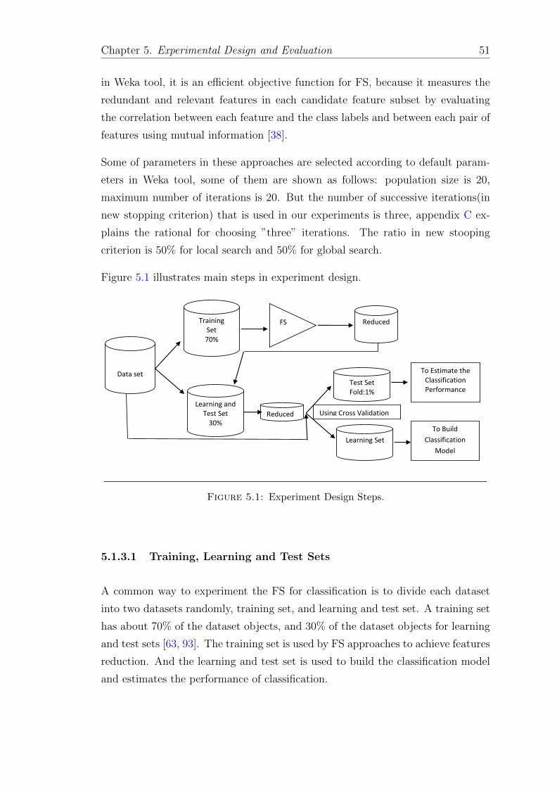
Chapter 5. Experimental Design and Evaluation 51
in Weka tool, it is an efficient objective function for FS, because it measures the
redundant and relevant features in each candidate feature subset by evaluating
the correlation between each feature and the class labels and between each pair of
features using mutual information [38].
Some of parameters in these approaches are selected according to default param-
eters in Weka tool, some of them are shown as follows: population size is 20,
maximum number of iterations is 20. But the number of successive iterations(in
new stopping criterion) that is used in our experiments is three, appendix C ex-
plains the rational for choosing ”three” iterations. The ratio in new stooping
criterion is 50% for local search and 50% for global search.
Figure 5.1 illustrates main steps in experiment design.
Training Set 70%
Data set
Learning and Test Set
30% Reduced
To Build
Classification
Model
FS Reduced
Set
Test Set Fold:1%
Learning Set
Using Cross Validation
To Estimate the Classification Performance
Figure 5.1: Experiment Design Steps.
5.1.3.1 Training, Learning and Test Sets
A common way to experiment the FS for classification is to divide each dataset
into two datasets randomly, training set, and learning and test set. A training set
has about 70% of the dataset objects, and 30% of the dataset objects for learning
and test sets [63, 93]. The training set is used by FS approaches to achieve features
reduction. And the learning and test set is used to build the classification model
and estimates the performance of classification.

Chapter 5. Experimental Design and Evaluation 52
In this work, we use K-fold cross-validation [94] that as is implemented in the
Weka tool to split the learning and test set into two disjoint sets to build the
classification model and estimate the classification performance. When an object
belongs to the test set, its class is hidden from the classification model built based
on the learning set only. In particular, K-fold cross-validation splits the learning
and test set into K subsets, then learning set is created on K-1 subsets, and test
set is created on the remaining subset, the size of k is 1% from learning and test
set. the process is repeated with several partitions to calculate the classification
performance.
5.1.3.2 Feature Reduction
We found, running the experiments five times was sufficient to obtain a good
comparison results between the two. Running the experiments longer than five
times did not provide additional value of comparison. Number of selected features
(features subset), and computational time are recorded for each run. In the next
step, run that achieved best classification accuracy is selected. Also PSO and
genetic approaches are run for each training set to achieve good feature reduction,
the number of selected features are recorded for each run. Remember, MBCSFS is
implemented in different environment from PSO [39], and genetic [37] approaches.
According to [3] DT and NB are common classification algorithms that are used
to estimate the classification performance, DT and NB are two algorithms from
top ten data mining algorithms, and they do not need complex initial parameters
[46]. For this, we use DT ”J48”[41] and NB[42] classification algorithms which
are implemented with Weka tool to measure the classification performance for
all approaches that are used in our experiments by applying these classification
algorithms on each reduced learning set to build the classification model that is
applied on test set to measure the classification performance. Also we measure
the classification performance for all datasets before and after FS.
5.2 Results and Discussion
In this section, MBCSFS is compared to BCSFS and other FS approaches, Table
5.2 shows the results of the comparison between the MBCSFS and BCSFS. Table

Chapter 5. Experimental Design and Evaluation 53
5.3 shows the computational time for MBCSFS and BCSFS approaches. Table
5.4 shows the smallest feature subset which is converged by BCSFS. Comparison
between 3OG and traditional objective functions is found in table 5.5. Table 5.6
compares the performance of MBCSFS for FS to genetic and PSO approaches.
Differences in accuracy is considered significant when it is more than 5% [91], and
it is considered the same when it is less than 1%[63].
5.2.1 Comparisons between MBCSFS and BCSFS
Table 5.2 shows the experimental results of MBCSFS and BCSFS with sixteen
datasets. We note, no significant difference between average of precision and aver-
age of recall, for this, accuracy is enough to evaluate the classification performance
for most datasets which are used in experiments. Following paragraphs discuss
these results.
Nominal Datasets . Table 5.2, Figure 5.2 show that MBCSFS and BCSFS
achieve the same size reduction, DT accuracy, and NB accuracy for congressional
voting records dataset. In Mushroom, Soybean (small), Lung Cancer datasets,
MBCSFS and BCSFS achieve better or roughly same DT accuracy, and NB accu-
racy, but MBCSFS achieves significant size reduction compared to BCSFS. The
main reasons for these results are: 3OG and traditional objective functions [19]
have roughly the same efficiency for nominal datasets. Also MBCSFS convergence
is better when the number of available features is more than 20 features, and the
best feature subset is less than quarter of available features, see section 5.3.3. For
this, MBCSFS achieves better reduction
Mixed Datasets Table 5.2, figure 5.3 show MBCSFS achieves better feature
reduction in all mixed datasets compared to BCSFS. In zoo dataset, MBCSFS
achieves less size reduction, but it improves the classification accuracy (DT ac-
curacy=13%, NB accuracy=26.7%). MBCSFS achieves the same size reduction,
and significantly better classification accuracy according to DT and NB compared
to BCSFS in Hepatitis and German Credit Data. But in Dermatology dataset,
MBCSFS achieves better size reduction and classification accuracy (DT and NB)
than BCSFS. Reasons for these results, 3OG objective function is more efficient
than traditional objective function for mixed datasets (number of distinct values

Chapter 5. Experimental Design and Evaluation 54
Dataset Method Size SR% Decision Tree % Naive Bayes %
Acc. Prec. Rec. DA Acc. Prec. Rec. DA
Nominal Datasets
Congressional Voting Records
All 16 96.7 96.8 96.8 90.1 90.5 90.1
MBCSFS 6 62.50 95.38 95.6 95.4 -1.32 94.6 94.6 94.6 4.5
BCSFS 6 62.50 95.38 95.6 95.4 -1.32 94.6 94.6 94.6 4.5
Mushroom
All 22 100 100 100 95.8 96 95.8
MBCSFS 4 81.82 98.4 98.5 98.4 -1.6 98.3 98.4 98.3 2.5
BCSFS 6 72.73 99.7 99.8 99.8 -0.3 98.1 98.3 98.2 2.3
Soybean(small)
All 35 95.7 96.5 95.7 97.8 98.1 97.9
MBCSFS 4 88.57 85.7 74.6 85.7 -10 100 100 100 2.2
BCSFS 15 71.43 85.7 75.5 85.7 -10 92.8 94 92.9 -5
Lung Cancer
All 56 50 50 50 56.2 55.3 56.3
MBCSFS 7 83.93 66.6 75.6 66.7 16.6 66.6 66.7 66.7 10.4
BCSFS 18 67.86 37.5 31.3 37.5 -12.5 62.5 39.1 62.5 6.3
Mixed Datasets
Zoo
All 17 93 95 93 94 94.6 94.1
MBCSFS 7 58.8 93 95 93 0 96.7 97.8 96.7 2.7
BCSFS 5 70.59 80 70 80 -13 70 70.6 70 -24
Hepatitis
All 19 80 80.2 80 83.2 84.1 83.2
MBCSFS 4 78.94 84.7 86.9 86.4 4.7 86.9 86.6 86.9 3.7
BCSFS 4 78.94 71.7 68.4 71.7 -8.3 73.9 72 73.9 -9.3
German Credit Data
All 20 71.2 69.4 71.1 35.1 74.7 35.1
MBCSFS 6 70.00 68 67.3 68 -3.2 71.3 69.8 71.3 36.2
BCSFS 6 70.00 67.3 62.1 67.3 -3.9 68 64.5 68 32.9
Dermatology
All 34 95.9 96 95.9 97.5 97.7 97.5
MBCSFS 10 70.59 93.6 94.7 93.6 -2.3 98.1 98.4 98.2 0.6
BCSFS 12 64.71 88.1 88.8 88.2 -7.8 93.6 94.1 93.6 -3.9
Numerical Datasets
Breast Cancer Wisconsin (Original)
All 9 93.9 93 93 96.1 96.3 96.1
MBCSFS 3 66.67 97.6 97.6 97.6 3.7 98.1 98.1 98.1 2
BCSFS 3 66.67 97.6 97.6 97.6 3.7 98.1 98.1 98.1 2
Wine
All 13 91.5 91.6 91.6 97.7 97.8 97.8
MBCSFS 3 76.92 87.3 87.3 87.1 -4.2 94.4 94.9 94.5 -3.3
BCSFS 2 84.62 83 82.9 83 -8.5 84.9 84.8 84.9 -12.8
Segment
All 19 96.4 96.4 96.4 81.2 83.3 81.3
MBCSFS 3 84.21 92.65 92.9 92.7 -3.75 83.1 82.9 83 1.9
BCSFS 6 68.42 80.5 80.4 80.6 -15.9 67.8 67.8 67.6 -13.4
Spectf
All 44 66.25 67.1 66.3 80 82 80
MBCSFS 6 86.3 75 75.7 75 8.75 83.33 84.3 83.3 3.33
BCSFS 15 65.91 62.5 65.1 62.5 -3.75 75 75.7 75 -5
Connectionist Bench (Sonar)
All 60 70.2 70.2 70.2 67.3 67.3 66.9
MBCSFS 13 78.33 79 78.9 79 8.7 67.7 67.4 67.7 0.4
BCSFS 22 63.33 72.5 72.3 72.6 2.31 70.9 75 71 3.6
Libras Movement
All 90 64.4 65.8 64.4 62.2 63.6 62.2
MBCSFS 7 92.22 60.5 60.6 60.6 -3.9 62.9 63.3 63 0.7
BCSFS 37 58.89 45.3 43.5 45.4 -19.1 51.8 56.2 51.9 -10.4
Musk (Version 1)
All 168 100 100 100 76.8 77.5 76.9
MBCSFS 7 95.83 96.2 97.7 96.2 -3.8 84.6 85.3 84.6 7.8
BCSFS 71 57.74 56.6 32.1 56.6 -43.4 69.9 69.9 69.9 -6.9
ISOLET-test
All 617 78 78.3 78.1 83.7 84.8 83.8
MBCSFS 51 91.73 76.2 76.4 75.9 -1.8 80.3 81.4 80.4 -3.4
BCSFS 283 54.13 64.3 64.9 64.3 -13.7 73.2 75.8 73.3 -10.5
All: Original Datasets. Size: Number of features. SR: Percentage of size reduction against all features Acc: Accuracy. Prec: Precession
Average. Rec: Recall Average. DA: Difference accuracy between accuracy of all features and accuracy of feature subset
Table 5.2: Results of BCSFS and MBCSFS.

Chapter 5. Experimental Design and Evaluation 55
in their features is different), MBCSFS is more efficient than BCSFS when the
number of available features is more than 20 features (dermatology dataset).
Figure 5.2: Comparisons Between MBCSFS and BCSFS for NominalDatasets(SR% and Classification Accuracy).
Figure 5.3: Comparisons Between MBCSFS and BCSFS for MixedDatasets(SR% and Classification Accuracy).
Numerical Datasets. According to Table 5.2, figure 5.4, MBCSFS and BCSFS
achieve the same feature reduction in Breast Cancer Wisconsin (Original) dataset,
because the number of available features is 9 (less than 20 features), and the
number of distinct values of its features is the same. In wine dataset, MBCSFS
achieves less size reduction, but it achieves significant improvement of classification
accuracy (DT and NB) compared to BCSFS. Main reason for this, 3OG objective
function is more efficient than traditional objective function for this dataset which
its features have different number of distinct values. In ISOLET dataset, BCSFS
failed to achieve the feature reduction, it selects around half number of available
features compared to MBCSFS which selects 8% from available features without
significant classification accuracy reduction. High number of distinct values (close

Chapter 5. Experimental Design and Evaluation 56
to total number of objects) for most of this dataset’s features, and the BCSFS’s
weak convergence are two main reasons for this results. High number of distinct
values and number of selected features make the RSTDD full dependency (100%)
for feature subsets which makes the BCSFS convergence uses local update only to
update the population of solutions, and this means, BCSFS is trapped into local
optimal.
Figure 5.4: Comparisons Between MBCSFS and BCSFS for NumericalDatasets(SR% and Classification Accuracy).
In remaining datasets, MBCSFS achieves better significant size reduction than
BCSFS (from 15.7% to 38.1%), with significant improvement in the classification
accuracy according to DT and NB(except sonar dataset, there is no significant
reduction of classification accuracy according to NB). MBCSFS has better efficient
convergence than BCSFS, especially when the number of available features for
these datasets is more than 20 features. Also 3OG objective is more efficient than
traditional objective function when the datasets have different number of distinct
values in their features
Finally, MBCSFS and BCSFS have the same efficiency when they are applied
on datasets that have less than 20 features, and their features have roughly the
same number of distinct values. But MBCSFS is more efficient than BCSFS when
they are applied on datasets that have more than 20 features, and their features
have different number of unique values. According to balancing between the size
reduction and classification accuracy, MBCSFS is more efficient than BCSFS in 14
datasets, and both approaches have the same efficiency in remaining two datasets.

Chapter 5. Experimental Design and Evaluation 57
5.2.2 Analysis of Computational Time
Table 5.3 shows the computational time of BCSFS and MBCSFS in seconds for
each dataset. Most of their computational time was spent in the objective func-
tion procedures such as calculating the number of distinct values and dependency
degree. Objective function runs twenty times (population size.) in each iteration.
In spite of the extra time needed for the new objective function that is used in
MBCSFS, MBCSFS took less time (about 34.4% from BCSFS time) than BCSFS
in all datasets, see figure 5.5. The main reason for this difference is that less num-
ber of iterations is needed in MBCSFS to reach to best feature subset, because
MBCSFS has fast and efficient convergence compared to BCSFS, and MBCSFS
stops when three successive iterations do not improve the value of objective func-
tion, but the BCSFS continues searching for best solution until it reaches maximum
number of iterations (20 iterations).
Dataset BCSFS MBCSFS
Itr. # Time(S) Time(S) For Convergence Itr. # Time(S)
Breast Cancer Wisconsin (Original)
7 3.68599 1.682 4 1.4092
Wine 10 1.053916 0.642 6 0.551574
Hepatitis 12 0.95728 0.7490 6 0.440
Congressional Voting Records 4 1.864377 0.6159 2 0.4217
Zoo 13 0.574956 0.532 4 0.240
Segment 18 13.07107 12.78 4 5.010
German Credit Data 7 7.49066 3.31 1 1.644
Mushroom 12 63.00201 50.46 3 19.73
Dermatology 3 5.51263 1.355 2 1.496
Soybean(small) 8 0.696 0.403 4 0.271
Spectf 13 1.45408 1.216 7 0.824
Lung Cancer 5 0.861 0.287 1 0.184
Connectionist Bench (Sonar) 19 3.064 2.93 3 0.894
Libras Movement 9 6.336 3.793 3 2.033
Musk (Version 1) 14 12.624 10.59 9 9.715
ISOLET-test 1 168.7582 16.091 3 55.398
Itr. #: Number of iterations needed to find the solution. Time(S): Time in seconds needed for approach
(20iterationas) to find the best feature subset. Time(S) for convergence: Time in seconds for BCSFS needed for
number of iterations that found the best feature subset
Table 5.3: Computational Time of BCSFS and MBCSFS.

Chapter 5. Experimental Design and Evaluation 58
0
20
40
60
80
100
120
BCSFS MBCSFS
Figure 5.5: Time Difference Between MBCSFS and BCSFS (%).
5.2.3 Analysis of convergence
This section discusses the efficiency of MBCSFS convergence, table 5.2 shows
that MBCSFS can converge the datasets with different sizes (from 9 features to
617 features), but the BCSFS’s convergence efficiency decreases as the number of
features increases more than 20, and the best features subset is the one which has
less than quarter of available features, see table 5.4. BCSFS can select about the
quarter of available features when the size of dataset is less than or equal to 20,
for this, we can consider the BCSFS convergence is efficient for the datasets that
have less than 20 features. Also 4.3 discussed these results theoreticaly.
0
2
4
6
8
10
12
14
16
18
20
BCSFS- Itr. # MBCSFS- Itr. #
Figure 5.6: Number of iterations needed to reach the best features subset
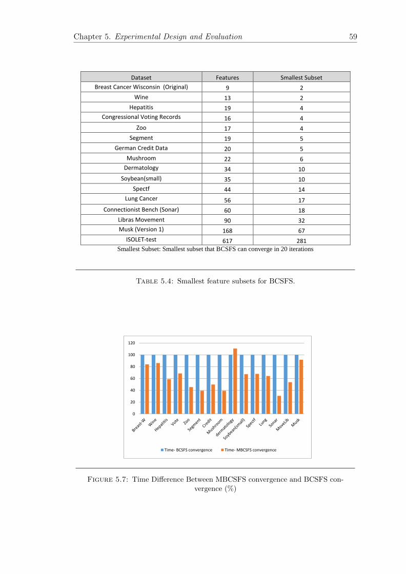
Chapter 5. Experimental Design and Evaluation 59
Dataset Features Smallest Subset
Breast Cancer Wisconsin (Original) 9 2
Wine 13 2
Hepatitis 19 4
Congressional Voting Records 16 4
Zoo 17 4
Segment 19 5
German Credit Data 20 5
Mushroom 22 6
Dermatology 34 10
Soybean(small) 35 10
Spectf 44 14
Lung Cancer 56 17
Connectionist Bench (Sonar) 60 18
Libras Movement 90 32
Musk (Version 1) 168 67
ISOLET-test 617 281 Smallest Subset: Smallest subset that BCSFS can converge in 20 iterations
Table 5.4: Smallest feature subsets for BCSFS.
0
20
40
60
80
100
120
Time- BCSFS convergence Time- MBCSFS convergence
Figure 5.7: Time Difference Between MBCSFS convergence and BCSFS con-vergence (%)

Chapter 5. Experimental Design and Evaluation 60
Now we evaluate the number of iterations needed to find the best feature subset.
Isolet-test dataset has numerical features that have very high number of distinct
values (low frequent values) in its features, and BCSFS selects about the half num-
ber of available features. This means, the value of traditional objective function
is 100%, which means BCSFS’s convergence use local update only to generate
new candidate feature subsets after the first iteration (BCSFS trapped into local
optimal). Table 5.3, and figure 5.6 show the number of iteration needed to find
the best features subset in both approaches. MBCSFS needs 57% iterations from
BCSFS iterations to find the best features subset in these datasets. Time for each
iteration in MBCSFS needs more time compared to BCSFS, because the 3OG
objective function cost more than traditional objective function[19], in general
MBCSFS convergence needs less time compared to BCSFS convergence ,because
it needs less number of iteration to find the best feature subset.
Figure 5.7 shows the time difference in percentage for convergence for both ap-
proaches. MBCSFS convergence needs less time compared to BCSFS convergence
in 14 datasets, because MBCSFS needs less significant number of iterations to
converge the search space in these datasets compared to BCSFS, but in dermatol-
ogy, the difference in number of iterations between them is little( one iteration),
for this, MBCSFS needs a little bit more time compared to BCSFS to find the
best feature subset. But in isolet-test dataset, BCSFS failed to achieve feature
reduction
5.2.4 Analysis of New Objective Function ”3OG”
To evaluate the new objective function ”3OG”, traditional objective function[19] is
combined to MBCSFS instead of 3OG objective function to construct MBCSFS T
approach which is implemented with PHP language, and it run five times for each
training set, then the classification performance are measured using NB and DT
that are implemented in Weka tool. Table 5.5 shows the experimental results of
MBCSFS and MBCSFS T.
According to table 5.5, and figure 5.8, 3OG objective function and traditional
objective function [19] have the same efficiency when they are applied on the
nominal datasets that have the same or roughly same number of distinct values in
their features.
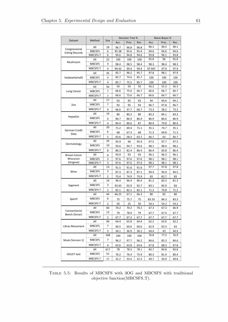
Chapter 5. Experimental Design and Evaluation 61
Dataset Method Size Decision Tree % Naive Bayes %
Acc. Prec. Rec. Acc. Prec. Rec.
Congressional Voting Records
All 16 96.7 96.8 96.8 90.1 90.5 90.1
MBCSFS 6 95.38 95.6 95.4 94.6 94.6 94.6
MBCSFS-T 6 94.6 94.8 94.6 93.8 94.1 93.8
Mushroom
All 22 100 100 100 95.8 96 95.8
MBCSFS 4 98.4 98.5 98.4 98.3 98.4 98.3
MBCSFS-T 4 99.42 99.4 99.4 97.947 97.9 97.9
Soybean(small)
All 35 95.7 96.5 95.7 97.8 98.1 97.9
MBCSFS 4 85.7 74.6 85.7 100 100 100
MBCSFS-T 4 85.7 75.5 85.7 100 100 100
Lung Cancer
All 56 50 50 50 56.2 55.3 56.3
MBCSFS 7 66.6 75.6 66.7 66.6 66.7 66.7
MBCSFS-T 7 66.6 75.6 66.7 66.6 66.7 66.7
Zoo
All 17 93 95 93 94 94.6 94.1
MBCSFS 7 93 95 93 96.7 97.8 96.7
MBCSFS-T 4 66.6 47.7 66.7 73.3 58.2 73.3
Hepatitis
All 19 80 80.2 80 83.2 84.1 83.2
MBCSFS 4 84.7 86.9 86.4 86.9 86.6 86.9
MBCSFS-T 4 84.4 86.6 87 80.4 79.8 80.4
German Credit Data
All 20 71.2 69.4 71.1 35.1 74.7 35.1
MBCSFS 6 68 67.3 68 71.3 69.8 71.3
MBCSFS-T 5 63.6 58.3 63.7 66.7 63 66.7
Dermatology
All 34 95.9 96 95.9 97.5 97.7 97.5
MBCSFS 10 93.6 94.7 93.6 98.1 98.4 98.2
MBCSFS-T 8 86.3 82.4 86.4 86.4 83.8 86.4
Breast Cancer Wisconsin (Original)
All 9 93.9 93 93 96.1 96.3 96.1
MBCSFS 3 97.6 97.6 97.6 98.1 98.1 98.1
MBCSFS-T 3 97.6 97.6 97.6 98.1 98.1 98.1
Wine
All 13 91.5 91.6 91.6 97.7 97.8 97.8
MBCSFS 3 87.3 87.3 87.1 94.4 94.9 94.5
MBCSFS-T 2 75.4 74.9 75.9 83 82.7 83
Segment
All 19 96.4 96.4 96.4 81.2 83.3 81.3
MBCSFS 3 92.65 92.9 92.7 83.1 82.9 83
MBCSFS-T 2 82.1 82.1 82.1 71.2 70.8 71.2
Spectf
All 44 66.25 67.1 66.3 80 82 80
MBCSFS 6 75 75.7 75 83.33 84.3 83.3
MBCSFS-T 2 50 25 50 54.1 54.2 54.2
Connectionist Bench (Sonar)
All 60 70.2 70.2 70.2 67.3 67.3 66.9
MBCSFS 13 79 78.9 79 67.7 67.4 67.7
MBCSFS-T 2 67.7 67.2 67.7 67.7 67.7 67.7
Libras Movement
All 90 64.4 65.8 64.4 62.2 63.6 62.2
MBCSFS 7 60.5 60.6 60.6 62.9 63.3 63
MBCSFS-T 5 36.1 36.9 36.1 44.4 43 44.4
Musk (Version 1)
All 168 100 100 100 76.8 77.5 76.9
MBCSFS 7 96.2 97.7 96.2 84.6 85.3 84.6
MBCSFS-T 4 63.6 63.8 63.6 67.8 68.3 67.8
ISOLET-test
All 617 78 78.3 78.1 83.7 84.8 83.8
MBCSFS 51 76.2 76.4 75.9 80.3 81.4 80.4
MBCSFS-T 17 32.2 33.4 32.3 49.7 50.9 49.8
Table 5.5: Results of MBCSFS with 3OG and MBCSFS with traditionalobjective function(MBCSFS T).

Chapter 5. Experimental Design and Evaluation 62
Figure 5.8: MBCSFS vs MBCSFS T for Nominal Datasets (Accuracy, SR%).
Table 5.5 results, and figure 5.9 shows that 3OG objective function is more efficient
than traditional objective function for mixed and numerical datasets. 3OG helps
the MBCSFS to achieve size reduction without significant classification accuracy
reduction, but traditional objective function makes the BCSFS achieve significant
size reduction with significant reduction of classification accuracy. But in breast
cancer wisconsin (original) dataset, both objective functions have the same ef-
ficiency, because the features in this dataset have the same number of distinct
values.
Figure 5.9: MBCSFS vs MBCSFS T for Mixed and Numerical Datasets (Ac-curacy, SR%).
Generally, 3OG and traditional objective function have the same efficiency for
nominal datasets, and the datasets which their features have roughly the same
distinct of values. But the 3OG objective function is more efficient for mixed and
numerical datasets which their features have different number of distinct values.
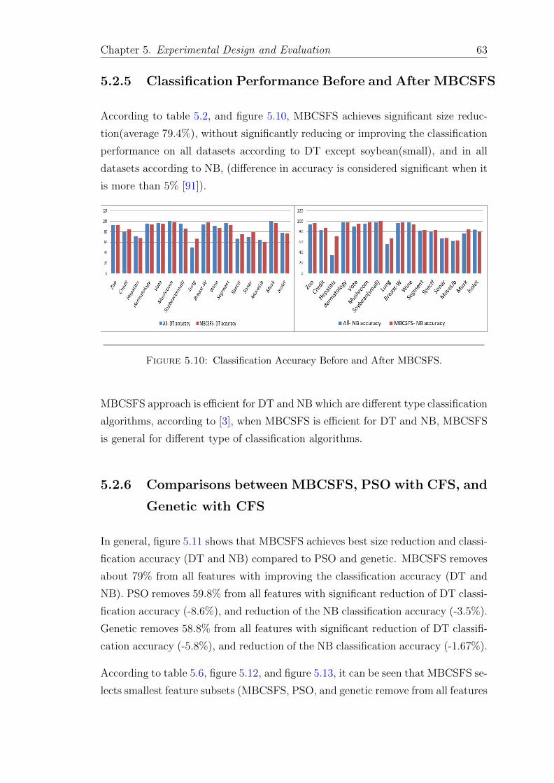
Chapter 5. Experimental Design and Evaluation 63
5.2.5 Classification Performance Before and After MBCSFS
According to table 5.2, and figure 5.10, MBCSFS achieves significant size reduc-
tion(average 79.4%), without significantly reducing or improving the classification
performance on all datasets according to DT except soybean(small), and in all
datasets according to NB, (difference in accuracy is considered significant when it
is more than 5% [91]).
Figure 5.10: Classification Accuracy Before and After MBCSFS.
MBCSFS approach is efficient for DT and NB which are different type classification
algorithms, according to [3], when MBCSFS is efficient for DT and NB, MBCSFS
is general for different type of classification algorithms.
5.2.6 Comparisons between MBCSFS, PSO with CFS, and
Genetic with CFS
In general, figure 5.11 shows that MBCSFS achieves best size reduction and classi-
fication accuracy (DT and NB) compared to PSO and genetic. MBCSFS removes
about 79% from all features with improving the classification accuracy (DT and
NB). PSO removes 59.8% from all features with significant reduction of DT classi-
fication accuracy (-8.6%), and reduction of the NB classification accuracy (-3.5%).
Genetic removes 58.8% from all features with significant reduction of DT classifi-
cation accuracy (-5.8%), and reduction of the NB classification accuracy (-1.67%).
According to table 5.6, figure 5.12, and figure 5.13, it can be seen that MBCSFS se-
lects smallest feature subsets (MBCSFS, PSO, and genetic remove from all features
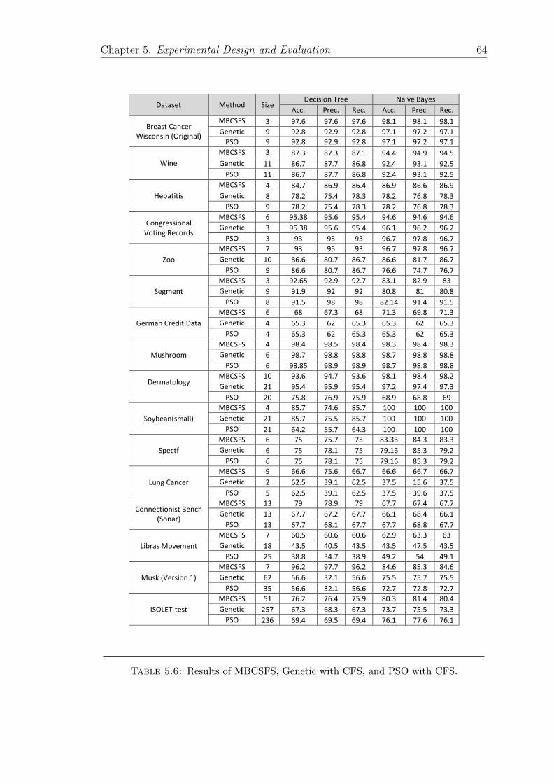
Chapter 5. Experimental Design and Evaluation 64
Dataset Method Size
Decision Tree Naive Bayes
Acc. Prec. Rec. Acc. Prec. Rec.
Breast Cancer Wisconsin (Original)
MBCSFS 3 97.6 97.6 97.6 98.1 98.1 98.1
Genetic 9 92.8 92.9 92.8 97.1 97.2 97.1
PSO 9 92.8 92.9 92.8 97.1 97.2 97.1
Wine
MBCSFS 3 87.3 87.3 87.1 94.4 94.9 94.5
Genetic 11 86.7 87.7 86.8 92.4 93.1 92.5
PSO 11 86.7 87.7 86.8 92.4 93.1 92.5
Hepatitis
MBCSFS 4 84.7 86.9 86.4 86.9 86.6 86.9
Genetic 8 78.2 75.4 78.3 78.2 76.8 78.3
PSO 9 78.2 75.4 78.3 78.2 76.8 78.3
Congressional Voting Records
MBCSFS 6 95.38 95.6 95.4 94.6 94.6 94.6
Genetic 3 95.38 95.6 95.4 96.1 96.2 96.2
PSO 3 93 95 93 96.7 97.8 96.7
Zoo
MBCSFS 7 93 95 93 96.7 97.8 96.7
Genetic 10 86.6 80.7 86.7 86.6 81.7 86.7
PSO 9 86.6 80.7 86.7 76.6 74.7 76.7
Segment
MBCSFS 3 92.65 92.9 92.7 83.1 82.9 83
Genetic 9 91.9 92 92 80.8 81 80.8
PSO 8 91.5 98 98 82.14 91.4 91.5
German Credit Data
MBCSFS 6 68 67.3 68 71.3 69.8 71.3
Genetic 4 65.3 62 65.3 65.3 62 65.3
PSO 4 65.3 62 65.3 65.3 62 65.3
Mushroom
MBCSFS 4 98.4 98.5 98.4 98.3 98.4 98.3
Genetic 6 98.7 98.8 98.8 98.7 98.8 98.8
PSO 6 98.85 98.9 98.9 98.7 98.8 98.8
Dermatology
MBCSFS 10 93.6 94.7 93.6 98.1 98.4 98.2
Genetic 21 95.4 95.9 95.4 97.2 97.4 97.3
PSO 20 75.8 76.9 75.9 68.9 68.8 69
Soybean(small)
MBCSFS 4 85.7 74.6 85.7 100 100 100
Genetic 21 85.7 75.5 85.7 100 100 100
PSO 21 64.2 55.7 64.3 100 100 100
Spectf
MBCSFS 6 75 75.7 75 83.33 84.3 83.3
Genetic 6 75 78.1 75 79.16 85.3 79.2
PSO 6 75 78.1 75 79.16 85.3 79.2
Lung Cancer
MBCSFS 9 66.6 75.6 66.7 66.6 66.7 66.7
Genetic 2 62.5 39.1 62.5 37.5 15.6 37.5
PSO 5 62.5 39.1 62.5 37.5 39.6 37.5
Connectionist Bench (Sonar)
MBCSFS 13 79 78.9 79 67.7 67.4 67.7
Genetic 13 67.7 67.2 67.7 66.1 68.4 66.1
PSO 13 67.7 68.1 67.7 67.7 68.8 67.7
Libras Movement
MBCSFS 7 60.5 60.6 60.6 62.9 63.3 63
Genetic 18 43.5 40.5 43.5 43.5 47.5 43.5
PSO 25 38.8 34.7 38.9 49.2 54 49.1
Musk (Version 1)
MBCSFS 7 96.2 97.7 96.2 84.6 85.3 84.6
Genetic 62 56.6 32.1 56.6 75.5 75.7 75.5
PSO 35 56.6 32.1 56.6 72.7 72.8 72.7
ISOLET-test
MBCSFS 51 76.2 76.4 75.9 80.3 81.4 80.4
Genetic 257 67.3 68.3 67.3 73.7 75.5 73.3
PSO 236 69.4 69.5 69.4 76.1 77.6 76.1
Table 5.6: Results of MBCSFS, Genetic with CFS, and PSO with CFS.

Chapter 5. Experimental Design and Evaluation 65
Figure 5.11: General Comparison between MBCSFS, PSO, and Genetic ap-proaches .
79.87%, 49.7%, and 46.8% respectively) without significant reduction of classifica-
tion performance (DT and NB) from available features on breast cancer wisconsin
(original), zoo, Hepatitis, mushroom, dermatology,Soybean(small) , libras move-
ment, musk (version 1), wine, segment, and ISOLET-test datasets.
0
20
40
60
80
100
120
MBCSFS-SR% PSO- SR% Genetic- SR%
Figure 5.12: SR% of MBCSFS, PSO, and Genetic .
In spectf, and connectionist bench (sonar) datasets, MBCSFS, PSO, and genetic
achieves the same size reduction, and three approaches achieve the same DT classi-
fication accuracy in spectf dataset, while MBCSFS improves the NB classification
accuracy, but PSO and genetic achieve reduction of NB classification accuracy
in the same dataset. In connectionist bench (sonar) MBCSFS achieves better
classification accuracy according to DT and NB.
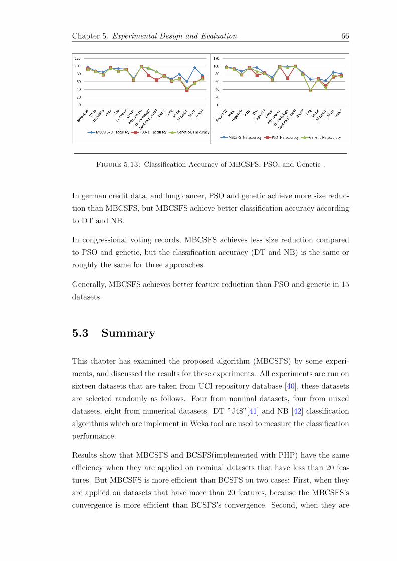
Chapter 5. Experimental Design and Evaluation 66
Figure 5.13: Classification Accuracy of MBCSFS, PSO, and Genetic .
In german credit data, and lung cancer, PSO and genetic achieve more size reduc-
tion than MBCSFS, but MBCSFS achieve better classification accuracy according
to DT and NB.
In congressional voting records, MBCSFS achieves less size reduction compared
to PSO and genetic, but the classification accuracy (DT and NB) is the same or
roughly the same for three approaches.
Generally, MBCSFS achieves better feature reduction than PSO and genetic in 15
datasets.
5.3 Summary
This chapter has examined the proposed algorithm (MBCSFS) by some experi-
ments, and discussed the results for these experiments. All experiments are run on
sixteen datasets that are taken from UCI repository database [40], these datasets
are selected randomly as follows. Four from nominal datasets, four from mixed
datasets, eight from numerical datasets. DT ”J48”[41] and NB [42] classification
algorithms which are implement in Weka tool are used to measure the classification
performance.
Results show that MBCSFS and BCSFS(implemented with PHP) have the same
efficiency when they are applied on nominal datasets that have less than 20 fea-
tures. But MBCSFS is more efficient than BCSFS on two cases: First, when they
are applied on datasets that have more than 20 features, because the MBCSFS’s
convergence is more efficient than BCSFS’s convergence. Second, when they are

Chapter 5. Experimental Design and Evaluation 67
applied on mixed and numerical datasets, because 3OG objective function in
MBCSFS is more efficient than traditional objective function in BCSFS . When
balancing between the size of reduction and classification accuracy, MBCSFS is
more efficient than BCSFS in 14 datasets, and both approaches have the same
efficiency in two datasets.
MBCSFS’s convergence is more efficient than BCSFS, and it needs 57% iterations
from BCSFS, also MBCSFS has efficient stopping criterion compared to BCSFS.
For this, MBCSFS took lesser time (about 34.4% from BCSFS time) than BCSFS.
3OG and traditional objective function have the same efficiency for nominal datasets,
and the datasets which their features have roughly the same number distinct of val-
ues. But the 3OG objective function is efficient for mixed and numerical datasets
which their features have different number of distinct values, compared to tra-
ditional objective function which is inefficient for them. Main reason for these
results, 3OG measure the frequent values in addition to RSTDD to guide the
search algorithm to best subset of features, but the traditional objective function
use RSTDD only.
MBCSFS is compared to genetic with CFS, and PSO with CFS which are imple-
mentd in Weka tool, MBCSFS achieves better feature reduction compared to PSO
and genetic on 15 datasets.

Chapter 6
Conclusion
This chapter conclude the thesis. A summary of literature review is presented
with focus on the main contributions, results, limitations and assumptions, and
future work.
6.1 Introduction
In our literature review, we focused on meta-heuristic filter FS approaches espe-
cially NIAs. Because NIAs approaches have been shown to have faster and more
efficient convergence compared to heuristic approaches which have slower and less
efficient convergence, and complete approaches which are very expensive. In the
exiting literature, there are many filter FS that used RSTDD to evaluate the can-
didate feature subsets that were generated from NIAs, that RSTDD relatively
cheaper, easier to implement, and does not need any preliminary or additional
information about data. The main drawback of these approaches is that of the
efficiency of convergence decreases as the number of features increases. And these
approaches are inefficient for mixed and numerical datasets [18–26]
.
Chapter 4 proposed a new filter FS for classification based on BCS , RSTDD and
distinct values to achieve feature reduction for nominal, mixed, and numerical
datasets with different characteristics of datasets especially different number of
features achieving in shorter computational time.
68

Chapter 6. Conclusion 69
The rest of this chapter presents the conclusion including contributions, summary
of results, limitation and assumptions. Also it presents potential research areas
for future work.
6.2 Contributions
The main contributions of this thesis, the development of new objective function,
and a modified BCS algorithm ( Chapter 4). These contribution are summarized
as bellow :
6.2.1 Objective function
A new objective function (3OG) has been developed to select the feature subset
that achieve maximum classification performance, and minimum number of fea-
tures for nominal, mixed, and numerical datasets, by combining RSTDD [19] and
distinct values. RSTDD measures the dependency between the feature subsets
and class labels. Distinct values measure the average number of distinct values in
feature subset to help the 3OG selects the subset that has more frequent values to
achieve more efficient results for mixed and numerical datasets as well as nominal
datasets. Finally, 3OG selects the minimum feature subset that has maximum
dependency to class labels (Maximum RSTDD) and maximum frequent values
(minimum number of distinct values) to achieve maximum classification perfor-
mance for nominal, mixed, and numerical datasets .
6.2.2 Modified Binary Cuckoo Search
The thesis developed a modified BCS algorithm by developing a new initialization,
global, local, switching, and stopping criterion mechanisms. Following paragraphs
show these points:
Initialization and Global Search: The initialization and global mechanisms
can significantly increase the performance of our work (MBCSFS) to reduce the
number of features and computational time.

Chapter 6. Conclusion 70
Our work divided the initialization and global mechanism to three parts to make
it faster as well as converge for datasets with different number of features. First
part converge small optimal solution (about 25% from total features). Second part
converge medium size(about 50% from total features). And the last part converge
large size of optimal solutions(about 75% from total features).
New Local Search: aims to increase the chance to find the global optimal so-
lution in a lesser number of iterations. The main idea is that the size of modifi-
cations of the current solutions decreases as the number of generations/iterations
increases.
New Switching Criterion: The switching criterion can improve the performance
of our work to solve local optimum problem.
We developed a new switching mechanism by dividing the nests equally for local
and global search, to guarantee that local and global searches are run in each iter-
ation. As shown, in chapter 5, this helped significantly improve the performance
of the algorithm.
New Stopping Criterion: Similarly the stopping criterion can significantly in-
crease the performance of our work to reduce the computational time.
We developed a new stopping criterion by stopping the algorithm after three suc-
cessive iterations if there is no improvement in the current solution.
Results show that our work achieved more efficient convergence for datasets that
have different number of features (up to 617 features), and it improve the compu-
tational time than BCS.
6.3 Results
Our work is evaluated by comparing it to the baseline algorithm (BCSFS), as well
as with genetic [37] with CFS and PSO [39] with CFS [38] approaches. Our work
and baseline approach were implemented in PHP, for the genetic with CFS and
PSO with CFS, the native Weka implementation was used. These approaches were
run on 16 datasets taken from UCI, and these approaches were evaluated by DT
and NB classification algorithms, using their native Weka implementation.

Chapter 6. Conclusion 71
Results show our work achieved better feature reduction on 14 datasets, and the
same feature reduction on two datasets compared to the baseline approach. Our
work took lesser time compared to the baseline approach on the datasets. Our
work also achieved significant size reduction without significant reduction in accu-
racy compared to classification accuracy for all features for nominal, mixed, and
numerical datasets(except soybean(small) according to DT). It also achieved bet-
ter feature reduction on 15 datasets compared to genetic and PSO approaches.
These results are described in the following points.
• Our work and baseline approach achieved the same size reduction for nominal
datasets that have less than 20 features, but ours achieved better feature re-
duction compared to BCSFS for all datasets that have more than 20 features.
This means, our work has better convergence compared to the baseline, and
3OG is more efficient( maximum classification performance with minimum
number of features) than the traditional objective function for mixed and
numerical datasets.
• Our work took less time (about 34.4% of BCSFS time) than the baseline
approach in all datasets, faster convergence, more efficient convergence, and
new stopping criterion for MBCSFS are the main reason for it.
• Our work achieved significant size reduction (about 79% on average), without
significantly reducing the classification accuracy on 15 datasets(less than 5%
from accuracy of all features ). Efficient convergence and efficient 3OG
objective function are the main reasons for it.
• Our work removed 79% from all features with improve the classification accu-
racy according to DT and NB . While PSO removed 59.8% from all features
with significant reduction of classification accuracy (DT:-8.6%, NB:-3.5%).
But genetic removed 58.8% from all features without significant reduction
of classification accuracy (DT:-5.8%, NB:-1.67%).
6.4 Limitations and Assumptions
16 datasets with different characteristics were selected to evaluate our work for
many characteristics such as difefrent number of features, different types, different

Chapter 6. Conclusion 72
number of classes, and different number of objects, but it is impossible that these
datasets cover all characteristics such as all number of features, all number of
objects, and all number of classes. This section explains some of assumptions and
limitations of our works as follows:
• We assumed all datasets do not have missing values.
• The maximum number of features that is used in the experiments is 617,
thus we could not ascertain how the algorithm would scale for datasets with
larger number of features.
• Our work achieved feature reduction for datasets that have from 2 to 26
classes, and from 36 to 8124 objects, similarly, we could not ascertain how
the algorithm would scale for datasets with larger number of objects or
classes.
6.5 Future Work
This section presents the main areas for future work for our work as follows:
• This thesis used distinct values to develop new objective function, but the
unique features, and the big difference between the numbers of distinct values
for each feature decrease the performance of our work. Therefore we need to
investigate the performance of our work by dealing these the two limitations
of our objective function.
• Maximum number of features are used in this thesis is 617, to investigate the
capability of our work on datasets that greater than 1000 features, alternative
initialization and global search would need to be further investigated to
develop a more dynamic approach to automatically subdivide the datasets
to search groups that provide optimal efficient computation.
Appendix A
Rough Set Theory
Rough Set Theory(RST) was developed by Zdzislaw Pawlak in the early 1982s
[15] as a mathematical tool that deals with classificatory analysis of data table.
Many researchers are very interested in RST, and applied it in many domains for
many reasons. First, it provides efficient methods for finding hidden patterns in
data. Second, it allows to reduce original data without additional information
about data. Third, It is easy to understand. Fourth, it allows to evaluate the
significance of data using data alone[16, 17]. Basic concepts of RST is discussed
below.
Information table or information system: Dataset in RST is called informa-
tion table or information system. Let I=(U,A), where I is information table/system
, U is a nonempty set of finite objects and A is a nonempty set of attributes/fea-
tures. In table A.1, {a,b,c,d,e} are features, but the features consist of four
conditional features and one decision feature(Class) D={e}. {0,1,2,3,4,5,6,7} are
objects[15–17].
Indiscernibility: Any subset P of A determines a binary relation IND(P) on U,
which is called an indiscernibility relation. Indiscernibility(IND) is equivalence
relation on the set U, where all the values are identical in relation to a subset of
attributes. For example, if P={b,c}, IND(P) creates the following partitions of U:
U/IND(P)
Positive region: Let P and Q be equivalence relations over U , then the positive
region contains all objects of U that can be classified to classes of U/Q using
information in attributes/features P [19,20.30,31]. For example, let P ={b,c} and
73
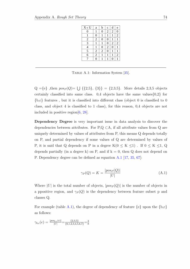
Appendix A. Rough Set Theory 74
X ϵ U a b c d e
0 1 0 2 2 0
1 0 1 1 1 2
2 2 0 0 1 1
3 1 1 0 2 2
4 1 0 2 0 1
5 2 2 0 1 1
6 2 1 1 1 2
7 0 1 1 0 1
Table A.1: Information System [35].
Q ={e} ,then posP (Q)=⋃{{2,5}, {3}} = {2,3,5}. More details 2,3,5 objects
certainly classified into same class. 0,4 objects have the same values{0,2} for
{b,c} features , but it is classified into different class (object 0 is classified to 0
class, and object 4 is classified to 1 class), for this reason, 0,4 objects are not
included in positive region[6, 28].
Dependency Degree is very important issue in data analysis to discover the
dependencies between attributes. For P,Q ⊂A, if all attribute values from Q are
uniquely determined by values of attributes from P, this means Q depends totally
on P, and partial dependency if some values of Q are determined by values of
P, it is said that Q depends on P in a degree K(0 ≤ K ≤1) . If 0 ≤ K ≤1, Q
depends partially (in a degree k) on P, and if k = 0, then Q does not depend on
P. Dependency degree can be defined as equation A.1 [17, 35, 67]:
γP (Q) = K =|posP (Q)||U |
(A.1)
Where |U | is the total number of objects, |posP (Q)| is the number of objects in
a ppositive region, and γP (Q) is the dependency between feature subset p and
classes Q.
For example (table A.1), the degree of dependency of feature {e} upon the {b,c}as follows:
γb,c(e) =|posb,c(e)|
|U | = {2,3,5}{0,1,2,3,4,5,6,7}=3
8

Appendix B
Levy Flights
In nature, many animals and insects search for food by moving to the next location
based on the current location. This behavior of search called levy flight that is
a special case of random walks where the step size has a Levy tailed probability
distribution to maximize the guarantee and speed of convergence [74]. Step sizes
is the main factor of the efficiency of levy flight search. Levy flight is modeled
in the equation B.1. Remember each solution must be a binary vector, but this
equation does not return a binary bit. In order to build a binary vector for each
solution, existing study uses equation B.3 and equation B.4 for each feature at
each new candidate solution.
𝑥𝑖,𝑗𝑡+1 = 𝑥𝑖,𝑗
𝑡 +α ⊕ L´evy(λ) (B.1)
L´evy ∼ u = t−λ (B.2)
Where xt+1(i,j) represents the jth egg(feature) at ith nest(solution) in iteration t , α is
the step size(α >0) scaling factor of the problem, In most cases, we can use α=1.
⊕ means entry-wise multiplications, and λ: Levy distribution coefficient (0 < λ ≤3). Random step length(Levy(λ) is calculated from power low by the equation
B.2.
75

Appendix B. Levy Flights 76
S(x(i,j) t+1 ) =
1
1+𝑒−𝑥𝑖,𝑗
𝑡+1 (B.3)
x(i,j) t+1 = (B.4)
1 , S(x(i,j) t+1 ) >σ
0 , Otherwise
Where σ ∈[0,1], in iteration t .

Appendix C
New Stopping Criterion
It is very difficult to determine if the algorithm finds the optimal feature subset
or not, because the evaluation of feature subset depends on its size and quality.
For this reason, most of existing approaches uses maximum iterations to stop the
algorithm. In most cases, this causes wasting much time without improving the
solutions.
Table C.1 shows our work searching for two datasets. First dataset is mushroom
which has 22 features and 8124 objects. Second dataset is libras lovement that has
90 features and 360 objects. Our work finds the best feature subset for mushroom
dataset in sixth iteration, and in the libras lovement dataset in third iteration,
while algorithm continue searching to reach the maximum number of iterations in
both datasets. This means, our work wastes much time without any use. Accord-
ing to results in table C.1, when three successive iterations do not improve the
current best solution, this means, there is no a chance to improve them, and the
algorithm must stop before reaching to maximum number of iterations.
77

Appendix C. New Stopping Criterion 78
Mushroom Dataset
Itr# Number of Selected Features Values of objective function “3OG”
1 6 0.7264
2 13 0.4086
3 6 0.7265
4 8 0.6358
5 5 0.7718
6 3 0.8627
7 7 0.6809
8 8 0.6355
9 7 0.6810
10 6 0.7263
11 6 0.7263
12 9 0.59014
13 10 0.5447
14 9 0.590
15 4 0.8170
16 5 0.7718
17 5 0.7720
18 11 0.4994
19 19 0.7266
Libras Movement Dataset
Itr# Number of Selected Features Values of objective function “3OG”
1 5 0.3255
2 7 0.3056
3 5 0.3494
4 7 0.3265
5 20 0.2783
6 9 0.33003
7 6 0.3209
8 20 0.26837
9 9 0.3130
10 5 0.31282
11 11 0.3012
12 19 0.278
13 7 0.325
14 4 0.320
15 21 0.279
16 10 0.3344
17 13 0.29368
18 10 0.31023
19 5 0.3426
Table C.1: Our Work Searching on Mushroom and Libras Movement Datasets.

Appendix D
Classifications of Dimensionality
Reduction
Dimintionality Reduction
Feature Selection
Ranked Approaches
Feature Subset Evaluation
Complete Approaches
Heuristic Approaches
Meta-heuristic Approaches
Nature Inspired
Approaches
Ant Colony Optimization
Particle Swarm Optimization
Artificial Bee Colony
Cuckoo Search
Binary Cuckoo Search
Non-nature Inspired
Approaches
Feature Extration/Transform
ation
Linear Approaches
Non-linear Approaches
Figure D.1: Classification of Dimensionality Reduction.
79

Bibliography
[1] Richard Jensen. Combining rough and fuzzy sets for feature selection. PhD
thesis, School of Informatics, University of Edinburgh, 2005.
[2] Oded Maimon and Lior Rokach. Introduction to knowledge discovery and
data mining. In Data Mining and Knowledge Discovery Handbook, pages
1–15. Springer, 2010.
[3] Huan Liu and Hiroshi Motoda. Feature selection for knowledge discovery and
data mining. Springer Science & Business Media, 1998.
[4] Pang-Ning Tan, Michael Steinbach, and Vipin Kumar. Introduction to data
mining. 1st. Boston: Pearson Addison Wesley. xxi, 2005.
[5] Huimin Zhao, Atish P Sinha, and Wei Ge. Effects of feature construction
on classification performance: An empirical study in bank failure prediction.
Expert Systems with Applications, 36(2):2633–2644, 2009.
[6] Daphne Koller and Mehran Sahami. Toward optimal feature selection. Stan-
ford InfoLab, 1996.
[7] Iffat A Gheyas and Leslie S Smith. Feature subset selection in large dimen-
sionality domains. Pattern recognition, 43(1):5–13, 2010.
[8] Nojun Kwak and Chong-Ho Choi. Input feature selection for classification
problems. Neural Networks, IEEE Transactions on, 13(1):143–159, 2002.
[9] Luiz S Oliveira, Robert Sabourin, Flavio Bortolozzi, and Ching Y Suen. Fea-
ture selection using multi-objective genetic algorithms for handwritten digit
recognition. In Pattern Recognition, 2002. Proceedings. 16th International
Conference on, volume 1, pages 568–571. IEEE, 2002.
[10] Manoranjan Dash and Huan Liu. Feature selection for classification. Intelli-
gent data analysis, 1(3):131–156, 1997.
80

Bibliography 81
[11] Lei Yu and Huan Liu. Efficient feature selection via analysis of relevance and
redundancy. The Journal of Machine Learning Research, 5:1205–1224, 2004.
[12] Pablo A Estevez, Michel Tesmer, Claudio A Perez, and Jacek M Zurada.
Normalized mutual information feature selection. Neural Networks, IEEE
Transactions on, 20(2):189–201, 2009.
[13] Zahra Beheshti and Siti Mariyam Hj Shamsuddin. A review of population-
based meta-heuristic algorithms. Int. J. Adv. Soft Comput. Appl, 5(1):1–35,
2013.
[14] El-Ghazali Talbi. Metaheuristics: from design to implementation, volume 74.
John Wiley & Sons, 2009.
[15] Zdzis law Pawlak. Rough sets. International Journal of Computer & Infor-
mation Sciences, 11(5):341–356, 1982.
[16] Zdzis law Pawlak. Rough sets: Theoretical aspects of reasoning about data,
volume 9. Springer Science & Business Media, 1991.
[17] Zdzis law Pawlak. Some issues on rough sets. In Transactions on Rough Sets
I, pages 1–58. Springer, 2004.
[18] Liangjun Ke, Zuren Feng, and Zhigang Ren. An efficient ant colony optimiza-
tion approach to attribute reduction in rough set theory. Pattern Recognition
Letters, 29(9):1351–1357, 2008.
[19] Richard Jensen and Qiang Shen. Finding rough set reducts with ant colony
optimization. In Proceedings of the 2003 UK workshop on computational
intelligence, volume 1, 2003.
[20] Majdi Mafarja and Derar Eleyan. Ant colony optimization based feature
selection in rough set theory. vol, 1:244–247.
[21] Xiangyang Wang, Jie Yang, Xiaolong Teng, Weijun Xia, and Richard Jensen.
Feature selection based on rough sets and particle swarm optimization. Pat-
tern Recognition Letters, 28(4):459–471, 2007.
[22] Hongyuan Shen, Shuren Yang, and Jianxun Liu. An attribute reduction of
rough set based on pso. In Rough Set and Knowledge Technology, pages 695–
702. Springer, 2010.

Bibliography 82
[23] H Hannah Inbarani, Ahmad Taher Azar, and G Jothi. Supervised hybrid
feature selection based on pso and rough sets for medical diagnosis. Computer
methods and programs in biomedicine, 113(1):175–185, 2014.
[24] Yurong Hu, Lixin Ding, Datong Xie, and Shenwen Wang. A novel discrete
artificial bee colony algorithm for rough set-based feature selection. Interna-
tional Journal of Advancements in Computing Technology, 4(6), 2012.
[25] N Suguna and K Thanushkodi. A novel rough set reduct algorithm for medical
domain based on bee colony optimization. arXiv preprint arXiv:1006.4540,
2010.
[26] Nambiraj Suguna and Keppana G Thanushkodi. An independent rough set
approach hybrid with artificial bee colony algorithm for dimensionality reduc-
tion. American Journal of Applied Sciences, 8(3):261, 2011.
[27] Zahra Beheshti and Siti Mariyam Hj Shamsuddin. A review of population-
based meta-heuristic algorithms. Int. J. Adv. Soft Comput. Appl, 5(1):1–35,
2013.
[28] Xin-She Yang and Suash Deb. Cuckoo search via levy flights. In Nature
& Biologically Inspired Computing, 2009. NaBIC 2009. World Congress on,
pages 210–214. IEEE, 2009.
[29] Sangita Roy and Sheli Sinha Chaudhuri. Cuckoo search algorithm using levy
flight: A review. I.J. Modern Education and Computer Science, 2013.
[30] K Waqas, R Baig, and S Ali. Feature subset selection using multi-objective
genetic algorithms. In Multitopic Conference, 2009. INMIC 2009. IEEE 13th
International, pages 1–6. IEEE, 2009.
[31] Douglas Rodrigues, Luis AM Pereira, TNS Almeida, Joao Paulo Papa,
AN Souza, Caio CO Ramos, and Xin-She Yang. Bcs: A binary cuckoo search
algorithm for feature selection. In Circuits and Systems (ISCAS), 2013 IEEE
International Symposium on, pages 465–468. IEEE, 2013.
[32] Mahmood Moghadasian and Seyedeh Parvaneh Hosseini. Binary cuckoo op-
timization algorithm for feature selection in high-dimensional datasets. In-
ternational Conference on Innovative Engineering Technologies, 2014.
[33] W Loh. Classification and regression tree methods. in’encyclopedia of statis-
tics in quality and reliability’(eds ruggeri, kenett, faltin) pp. 315-323, 2008.

Bibliography 83
[34] Gilbert Laporte and Ibrahim H Osman. Routing problems: A bibliography.
Annals of Operations Research, 61(1):227–262, 1995.
[35] Richard Jensen and Qiang Shen. Semantics-preserving dimensionality re-
duction: Rough and fuzzy-rough-based approaches. IEEE Transactions on
Knowledge and Data Engineering, 17(1):1, 2005.
[36] Guangming Lang, Qingguo Li, and Lankun Guo. Discernibility matrix simpli-
fication with new attribute dependency functions for incomplete information
systems. Knowledge and information systems, 37(3):611–638, 2013.
[37] David E Goldberg. Genetic algorithms in search, optimization and machine
learning addison-wesley, 1989. Reading, MA, 1989.
[38] Mark A Hall. Correlation-based feature selection for machine learning. PhD
thesis, The University of Waikato, 1999.
[39] Alberto Moraglio, Cecilia Di Chio, and Riccardo Poli. Geometric particle
swarm optimisation. In Genetic Programming, pages 125–136. Springer, 2007.
[40] Christopher J Merz and Patrick M Murphy. {UCI} repository of machine
learning databases. 1998.
[41] Steven L Salzberg. C4. 5: Programs for machine learning by j. ross quinlan.
morgan kaufmann publishers, inc., 1993. Machine Learning, 16(3):235–240,
1994.
[42] George H John and Pat Langley. Estimating continuous distributions in
bayesian classifiers. In Proceedings of the Eleventh conference on Uncertainty
in artificial intelligence, pages 338–345. Morgan Kaufmann Publishers Inc.,
1995.
[43] Zhiyong Lu, Duane Szafron, Russell Greiner, Paul Lu, David S Wishart, Brett
Poulin, John Anvik, Cam Macdonell, and Roman Eisner. Predicting subcellu-
lar localization of proteins using machine-learned classifiers. Bioinformatics,
20(4):547–556, 2004.
[44] E Costa, A Lorena, ACPLF Carvalho, and A Freitas. A review of performance
evaluation measures for hierarchical classifiers. In Evaluation Methods for
Machine Learning II: papers from the AAAI-2007 Workshop, pages 1–6, 2007.

Bibliography 84
[45] Foster Provost and Ron Kohavi. Guest editors’ introduction: On applied
research in machine learning. Machine learning, 30(2):127–132, 1998.
[46] Xindong Wu, Vipin Kumar, J Ross Quinlan, Joydeep Ghosh, Qiang Yang,
Hiroshi Motoda, Geoffrey J McLachlan, Angus Ng, Bing Liu, S Yu Philip,
et al. Top 10 algorithms in data mining. Knowledge and Information Systems,
14(1):1–37, 2008.
[47] Hussein Almuallim and Thomas G Dietterich. Learning boolean concepts in
the presence of many irrelevant features. Artificial Intelligence, 69(1):279–305,
1994.
[48] Kenji Kira and Larry A Rendell. The feature selection problem: Traditional
methods and a new algorithm. In AAAI, volume 2, pages 129–134, 1992.
[49] Nojun Kwak and Chong-Ho Choi. Input feature selection for classification
problems. Neural Networks, IEEE Transactions on, 13(1):143–159, 2002.
[50] A Wayne Whitney. A direct method of nonparametric measurement selection.
Computers, IEEE Transactions on, 100(9):1100–1103, 1971.
[51] Thomas Marill and David M Green. On the effectiveness of receptors in
recognition systems. Information Theory, IEEE Transactions on, 9(1):11–17,
1963.
[52] Martin Gutlein, Eibe Frank, Mark Hall, and Andreas Karwath. Large-scale
attribute selection using wrappers. In Computational Intelligence and Data
Mining, 2009. CIDM’09. IEEE Symposium on, pages 332–339. IEEE, 2009.
[53] Shih-Wei Lin, Kuo-Ching Ying, Shih-Chieh Chen, and Zne-Jung Lee. Parti-
cle swarm optimization for parameter determination and feature selection of
support vector machines. Expert systems with applications, 35(4):1817–1824,
2008.
[54] Rahul Karthik Sivagaminathan and Sreeram Ramakrishnan. A hybrid ap-
proach for feature subset selection using neural networks and ant colony op-
timization. Expert systems with applications, 33(1):49–60, 2007.
[55] Anuradha Purohit, Narendra S Chaudhari, and Aruna Tiwari. Construction
of classifier with feature selection based on genetic programming. In Evo-
lutionary Computation (CEC), 2010 IEEE Congress on, pages 1–5. IEEE,
2010.

Bibliography 85
[56] Jung-Yi Lin, Hao-Ren Ke, Been-Chian Chien, and Wei-Pang Yang. Classi-
fier design with feature selection and feature extraction using layered genetic
programming. Expert Systems with Applications, 34(2):1384–1393, 2008.
[57] Svante Wold, Kim Esbensen, and Paul Geladi. Principal component analysis.
Chemometrics and intelligent laboratory systems, 2(1):37–52, 1987.
[58] Kimberly Welsh Johnson and Naomi S Altman. Canonical correspondence
analysis as an approximation to gaussian ordination. Environmetrics, 10(1):
39–52, 1999.
[59] Darrall Henderson, Sheldon H Jacobson, and Alan W Johnson. The theory
and practice of simulated annealing. In Handbook of metaheuristics, pages
287–319. Springer, 2003.
[60] Mohammad-Reza Feizi-Derakhshi and Manizheh Ghaemi. Classifying dif-
ferent feature selection algorithms based on the search strategies. Interna-
tional Conference on Machine Learning, Electrical and Mechanical Engineer-
ing, 2014.
[61] Isabelle Guyon and Andre Elisseeff. An introduction to variable and feature
selection. The Journal of Machine Learning Research, 3:1157–1182, 2003.
[62] Roberto Ruiz, Jose C Riquelme, and Jesus S Aguilar-Ruiz. Fast feature rank-
ing algorithm. In Knowledge-Based Intelligent Information and Engineering
Systems, pages 325–331. Springer, 2003.
[63] Bing Xue, Mengjie Zhang, and Will N Browne. Particle swarm optimisa-
tion for feature selection in classification: Novel initialisation and updating
mechanisms. Applied Soft Computing, 18:261–276, 2014.
[64] Manoranjan Dash and Huan Liu. Feature selection for classification. Intelli-
gent data analysis, 1(3):131–156, 1997.
[65] Bing Xue, Mengjie Zhang, and Will N Browne. Multi-objective particle swarm
optimisation (pso) for feature selection. In Proceedings of the 14th annual con-
ference on Genetic and evolutionary computation, pages 81–88. ACM, 2012.
[66] Iztok Fister Jr, Xin-She Yang, Iztok Fister, Janez Brest, and Dusan Fister.
A brief review of nature-inspired algorithms for optimization. arXiv preprint
arXiv:1307.4186, 2013.

Bibliography 86
[67] Silvia Rissino and Germano Lambert-Torres. Rough set theory–fundamental
concepts, principals, data extraction, and applications. Data Mining and
Knowledge Discovery in Real Life Applications, page 438, 2009.
[68] Jan Kuratko and Stefan Ratschan. Combined global and local search for the
falsification of hybrid systems. In Formal Modeling and Analysis of Timed
Systems, pages 146–160. Springer, 2014.
[69] Marco Dorigo, Vittorio Maniezzo, and Alberto Colorni. Ant system: opti-
mization by a colony of cooperating agents. Systems, Man, and Cybernetics,
Part B: Cybernetics, IEEE Transactions on, 26(1):29–41, 1996.
[70] Riccardo Poli, James Kennedy, and Tim Blackwell. Particle swarm optimiza-
tion. Swarm intelligence, 1(1):33–57, 2007.
[71] S Binitha and S Siva Sathya. A survey of bio inspired optimization algo-
rithms. International Journal of Soft Computing and Engineering, 2(2):137–
151, 2012.
[72] B Basturk and Dervis Karaboga. An artificial bee colony (abc) algorithm for
numeric function optimization, ieee swarm intelligence symposium 2006, may
12–14, 2006. Indianapolis, Indiana, USA, 2006.
[73] DT Pham, A Ghanbarzadeh, E Koc, S Otri, S Rahim, and M Zaidi. The bees
algorithm-a novel tool for complex optimisation problems. In Proceedings of
the 2nd virtual international conference on intelligent production machines
and systems (IPROMS 2006), pages 454–459, 2006.
[74] Xin-She Yang and Suash Deb. Engineering optimisation by cuckoo search. In-
ternational Journal of Mathematical Modelling and Numerical Optimisation,
1(4):330–343, 2010.
[75] JB Jona and N Nagaveni. Ant-cuckoo colony optimization for feature selection
in digital mammogram. Pakistan journal of biological sciences: PJBS, 17(2):
266–271, 2014.
[76] Sanket Kamat and Asha Gowda Karegowda. A brief survey on cuckoo search
applications. International Conference On Advances in Computer & Com-
munication Engineering, 2014.

Bibliography 87
[77] Iztok Fister Jr, Xin-She Yang, Dusan Fister, and Iztok Fister. Cuckoo search:
a brief literature review. In Cuckoo search and firefly algorithm, pages 49–62.
Springer, 2014.
[78] Davar Giveki, Hamid Salimi, GholamReza Bahmanyar, and Younes
Khademian. Automatic detection of diabetes diagnosis using feature weighted
support vector machines based on mutual information and modified cuckoo
search. arXiv preprint arXiv:1201.2173, 2012.
[79] Milos Madic and Miroslav Radovanovic. Application of cuckoo search algo-
rithm for surface roughness optimization in co 2 laser cutting. Annals of the
Faculty of Engineering Hunedoara-International Journal of Engineering, 11
(1), 2013.
[80] Ivona Brajevic, Milan Tuba, and Nebojsa Bacanin. Multilevel image thresh-
olding selection based on the cuckoo search algorithm. In Advances in Sensors,
Signals, Visualization, Imaging and Simulation, 2012.
[81] M Prakash, R Saranya, K Rukmani Jothi, and A Vigneshwaran. An optimal
job scheduling in grid using cuckoo algorithm. Int. J. Comput. Sci. Telecomm,
3(2):65–69, 2012.
[82] Koffka Khan and Ashok Sahai. Neural-based cuckoo search of employee health
and safety (hs). Int. J. Intell. Syst. Appl.(IJISA), 5(2):76–83, 2013.
[83] Moe Moe Zaw and Ei Ei Mon. Web document clustering using cuckoo search
clustering algorithm based on levy flight. International Journal of Innovation
and Applied Studies, 4(1):182–188, 2013.
[84] Akajit Saelim, Suwanna Rasmequan, Pusit Kulkasem, Krisana Chinnasarn,
and Annupan Rodtook. Migration planning using modified cuckoo search
algorithm. In Communications and Information Technologies (ISCIT), 2013
13th International Symposium on, pages 621–626. IEEE, 2013.
[85] Ehsan Valian, Shahram Mohanna, and Saeed Tavakoli. Improved cuckoo
search algorithm for feedforward neural network training. International Jour-
nal of Artificial Intelligence & Applications, 2(3):36–43, 2011.
[86] S Walton, O Hassan, K Morgan, and MR Brown. Modified cuckoo search: a
new gradient free optimisation algorithm. Chaos, Solitons & Fractals, 44(9):
710–718, 2011.

Bibliography 88
[87] LAM Pereira, D Rodrigues, TNS Almeida, CCO Ramos, AN Souza, X-S
Yang, and JP Papa. A binary cuckoo search and its application for feature
selection. In Cuckoo Search and Firefly Algorithm, pages 141–154. Springer,
2014.
[88] JoaO P Papa, Alexandre X FalcaO, Victor Hugo C De Albuquerque, and Joao
Manuel RS Tavares. Efficient supervised optimum-path forest classification
for large datasets. Pattern Recognition, 45(1):512–520, 2012.
[89] Rafael Falcon, Marcio Almeida, and Amiya Nayak. Fault identification with
binary adaptive fireflies in parallel and distributed systems. In Evolutionary
Computation (CEC), 2011 IEEE Congress on, pages 1359–1366. IEEE, 2011.
[90] K Waqas, R Baig, and S Ali. Feature subset selection using multi-objective
genetic algorithms. In Multitopic Conference, 2009. INMIC 2009. IEEE 13th
International, pages 1–6. IEEE, 2009.
[91] Neil Parthalain, Qiang Shen, and Richard Jensen. A distance measure ap-
proach to exploring the rough set boundary region for attribute reduction.
Knowledge and Data Engineering, IEEE Transactions on, 22(3):305–317,
2010.
[92] Geoffrey Holmes, Andrew Donkin, and Ian H Witten. Weka: A machine
learning workbench. In Intelligent Information Systems, 1994. Proceedings of
the 1994 Second Australian and New Zealand Conference on, pages 357–361.
IEEE, 1994.
[93] Kevin K Dobbin and Richard M Simon. Optimally splitting cases for training
and testing high dimensional classifiers. BMC medical genomics, 4(1):31,
2011.
[94] Juan D Rodriguez, Aritz Perez, and Jose A Lozano. Sensitivity analysis of
k-fold cross validation in prediction error estimation. Pattern Analysis and
Machine Intelligence, IEEE Transactions on, 32(3):569–575, 2010.


