Modeling Terrestrial Ecosystem Distribution, Mapping Threats and Updating Protected Area
Information
Leonardo SotomayorSouth America Conservation Region
Terrestrial Ecosystems
• A layer of contiguous vegetation-based ecological systems as conservation targets
• Contracted NatureServe to develop the classification (Josse et al 2003), but had no map
• Project lead by Roger Sayre (now at USGS)• Data now being used for various applications
including preliminary biodiversity assessments and effective conservation measures
• Data is undergoing final updates and revisions prior to distribution
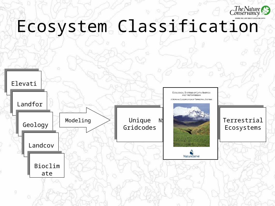
Ecosystem Classification
ElevationElevation
Unique Gridcodes
Unique Gridcodes
LandformLandform
GeologyGeology
LandcoverLandcover
BioclimateBioclimate
Terrestrial Ecosystems
Terrestrial Ecosystems
Modeling NS Classification
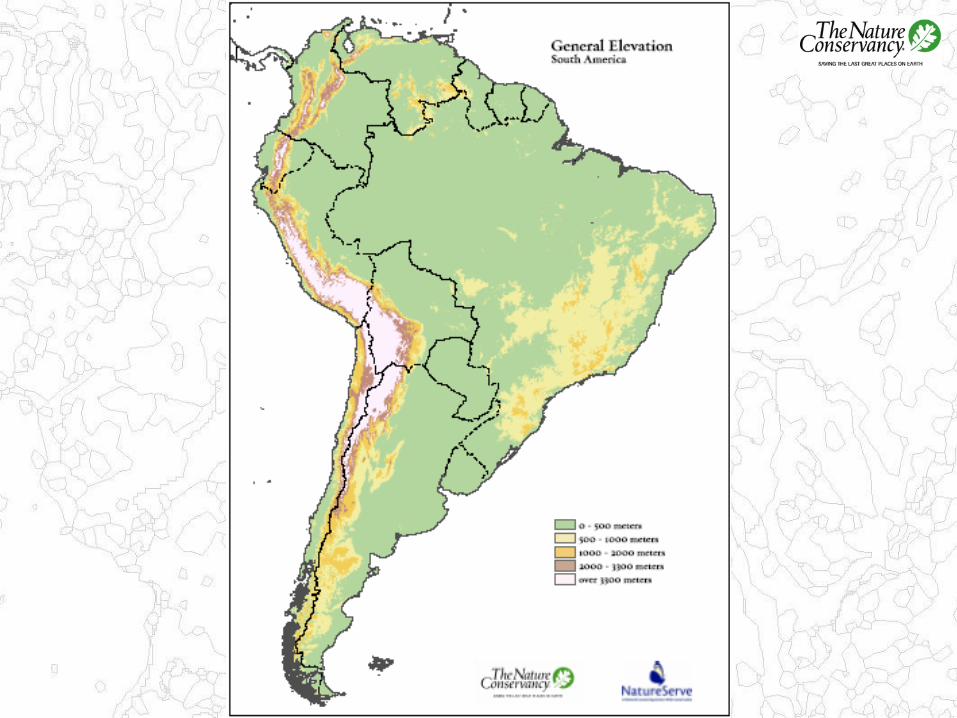
Elevation
• 450 Meter Digital Elevation Model Data (DEM) produced by WWF from 90 meter SRTM DEM data.
• Classification is based primarily on floristics:– 0 - 500m: corresponds to lowlands– 500 - 1000m: transitional mixed flora of the
piedmont, in the case of massive ridges like the Andes; or is already montane, with a different set of species, in the case of low ridges
– 1000 - 3300m: two life zones in the mountains, mostly forest covered
– Over 3300m: treelines for the Andes
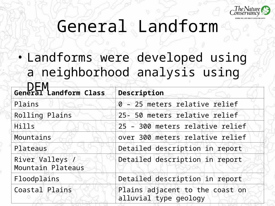
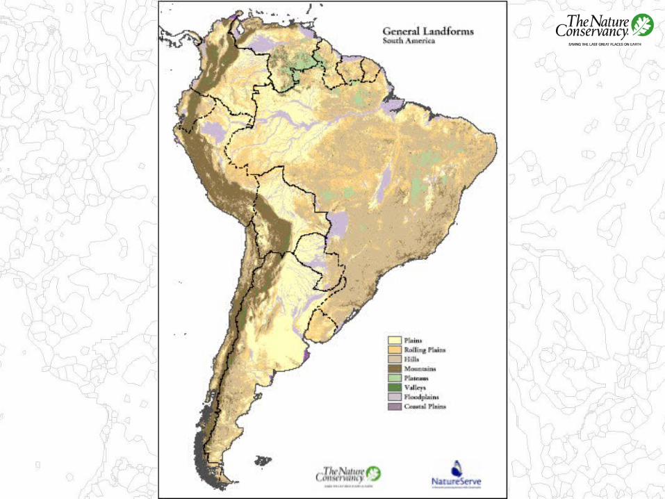
General Landform
• Landforms were developed using a neighborhood analysis using DEM
General Landform Class Description
Plains 0 – 25 meters relative relief
Rolling Plains 25- 50 meters relative relief
Hills 25 – 300 meters relative relief
Mountains over 300 meters relative relief
Plateaus Detailed description in report
River Valleys / Mountain Plateaus Detailed description in report
Floodplains Detailed description in report
Coastal Plains Plains adjacent to the coast on alluvial type geology
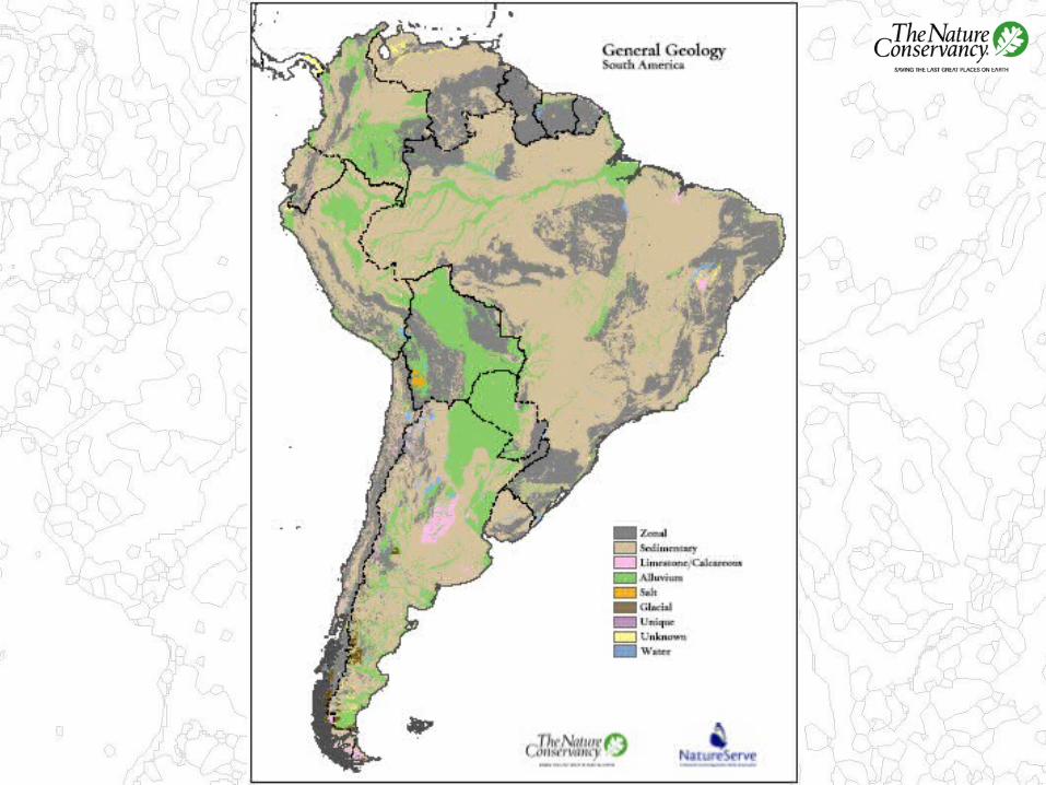
General Geology
• Detailed geology data was purchased from Geologic Data Systems Inc. (GDS).
• Compiled geological information from over 50 published maps to create a digital geology map of South America.
• Data for Brazil was compiled at 1:1,000,000 scale with the remainder of South America at 1:500,000 scale.
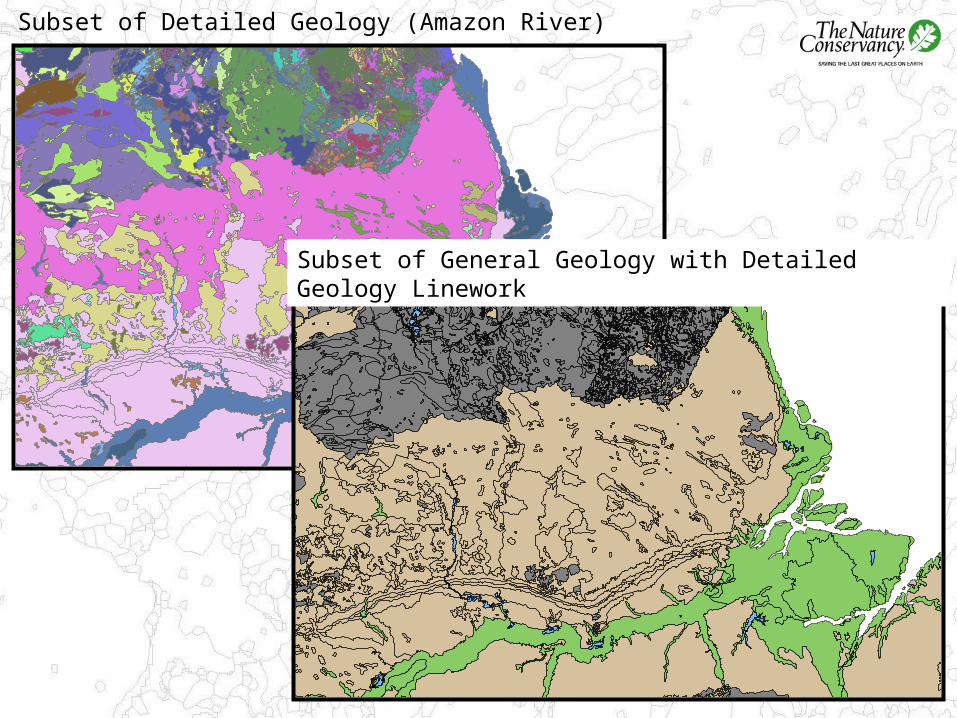
Subset of Detailed Geology (Amazon River)
Subset of General Geology with Detailed Geology Linework
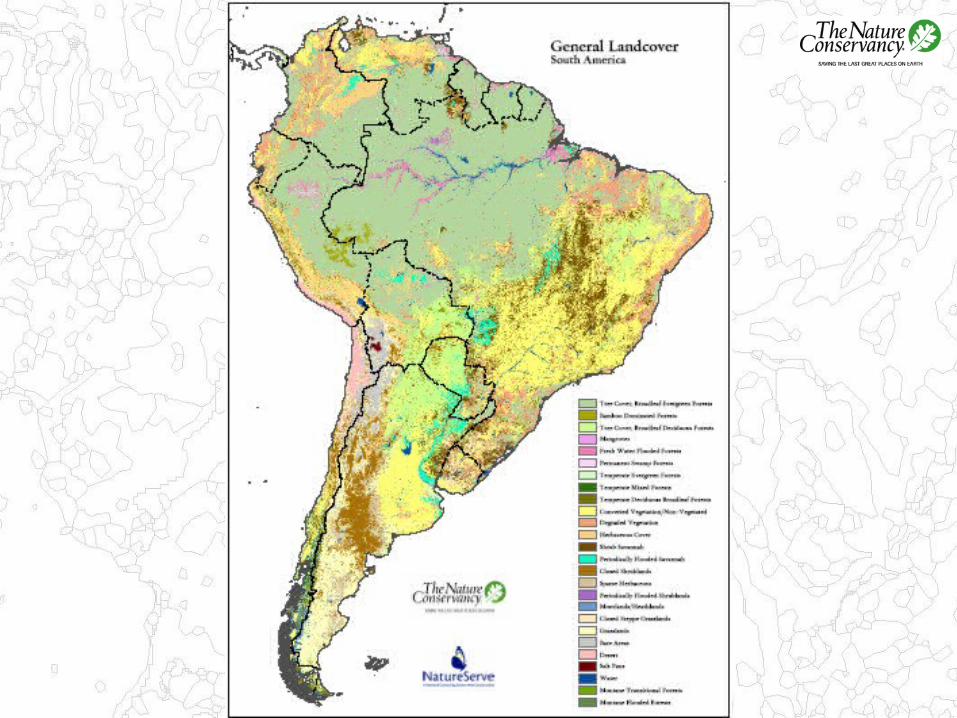
General Land Cover
• South America GLC 2000 (Global Land Cover 2000)
• 1 km resolution at the equator, resampled to 450 meters
• Generalized from 57 classes to 18 classes to reduce the natural complexity of the data
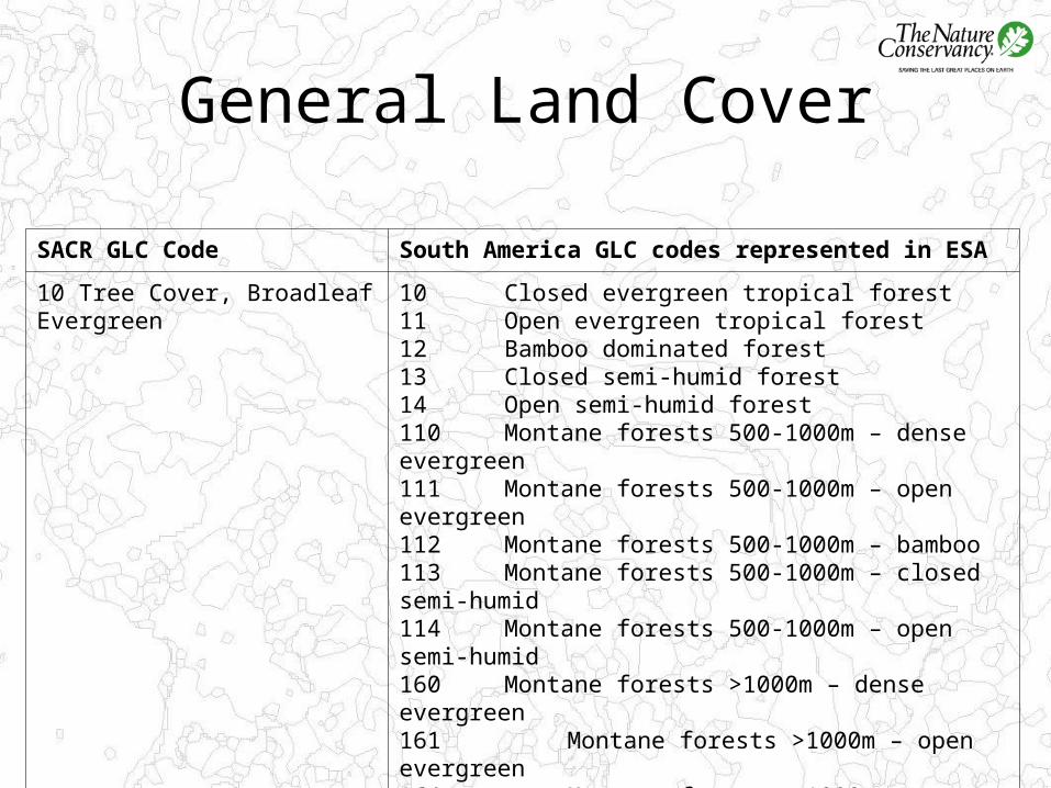
General Land Cover
SACR GLC Code South America GLC codes represented in ESA
10 Tree Cover, Broadleaf Evergreen 10 Closed evergreen tropical forest11 Open evergreen tropical forest12 Bamboo dominated forest13 Closed semi-humid forest14 Open semi-humid forest110 Montane forests 500-1000m – dense evergreen111 Montane forests 500-1000m – open evergreen112 Montane forests 500-1000m – bamboo 113 Montane forests 500-1000m – closed semi-humid114 Montane forests 500-1000m – open semi-humid160 Montane forests >1000m – dense evergreen161 Montane forests >1000m – open evergreen164 Montane forests >1000m – open semi humid
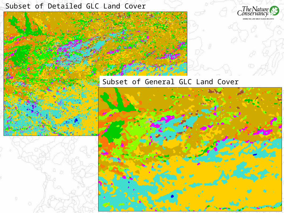
Subset of Detailed GLC Land Cover
Subset of General GLC Land Cover
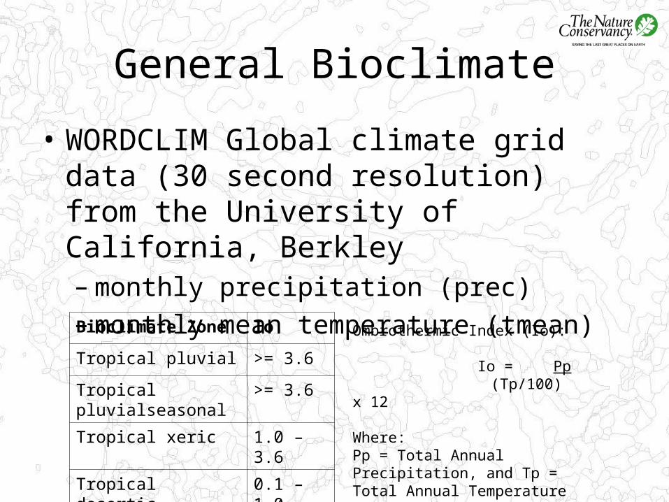
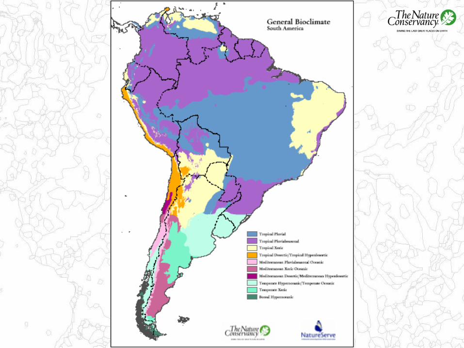
General Bioclimate
• WORDCLIM Global climate grid data (30 second resolution) from the University of California, Berkley– monthly precipitation (prec)– monthly mean temperature (tmean)Bioclimate Zone Io
Tropical pluvial >= 3.6
Tropical pluvialseasonal
>= 3.6
Tropical xeric 1.0 – 3.6
Tropical desertic 0.1 – 1.0
Tropical hyperdesertic < 0.1
Ombrothermic Index (Io):
Io = Pp (Tp/100) x 12
Where:Pp = Total Annual Precipitation, and Tp = Total Annual Temperature
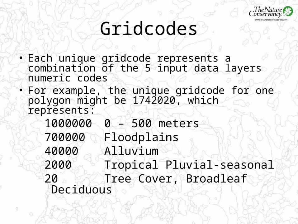
Gridcodes
• Each unique gridcode represents a combination of the 5 input data layers numeric codes
• For example, the unique gridcode for one polygon might be 1742020, which represents:
1000000 0 – 500 meters700000 Floodplains40000 Alluvium2000 Tropical Pluvial-seasonal20 Tree Cover, Broadleaf
Deciduous
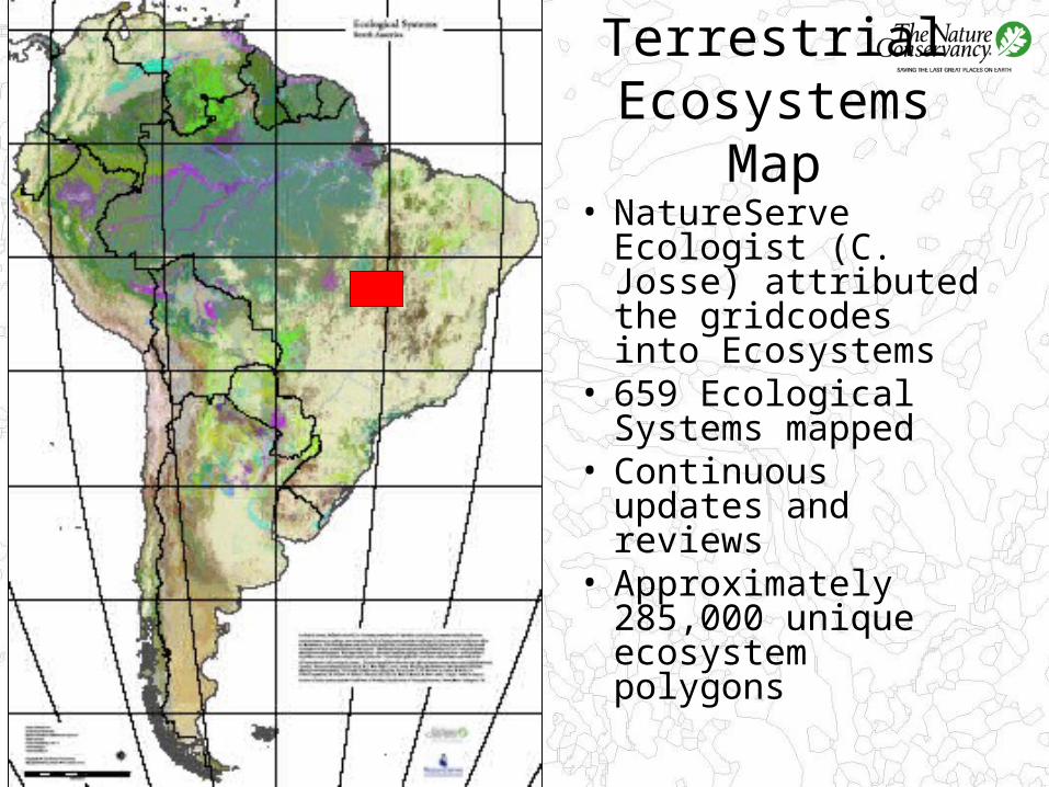
• NatureServe Ecologist (C. Josse) attributed the gridcodes into Ecosystems
• 659 Ecological Systems mapped
• Continuous updates and reviews
• Approximately 285,000 unique ecosystem polygons
Terrestrial Ecosystems Map
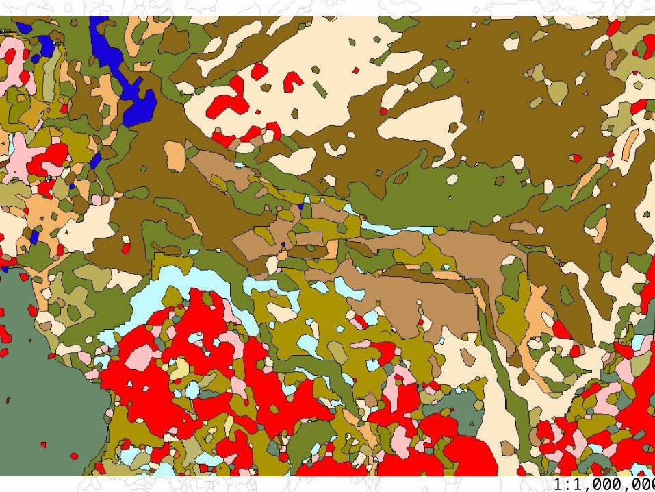
1:1,000,000
Current Human Activity
South America Threat to Biodiversity Assesment
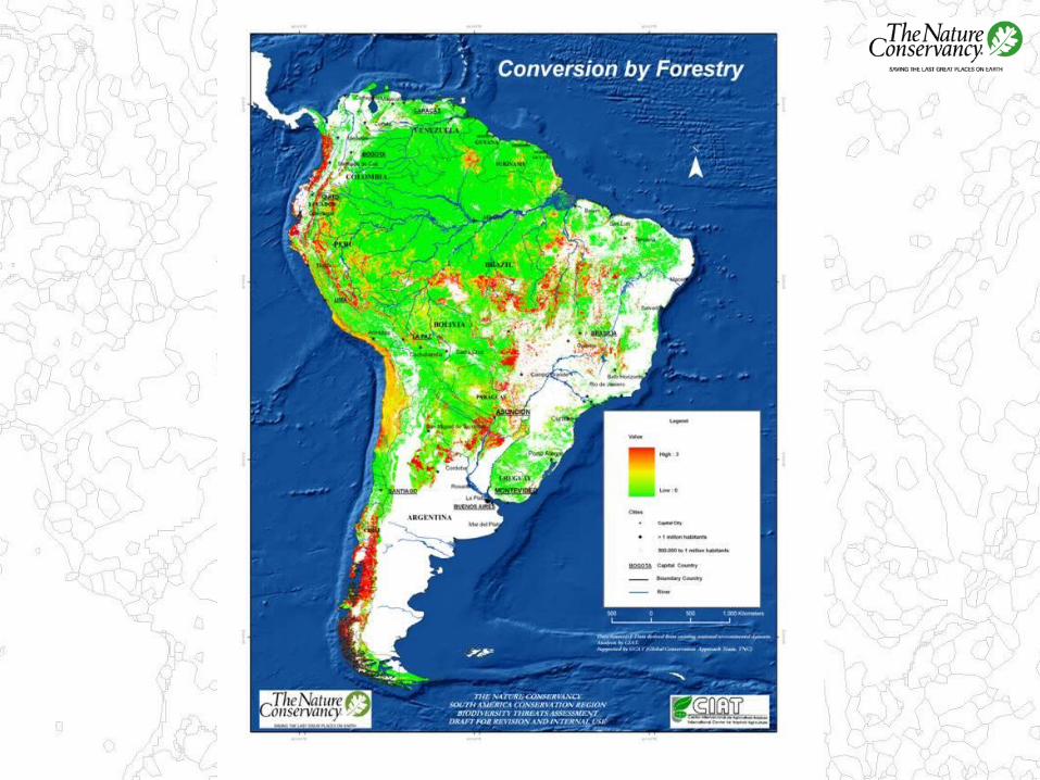
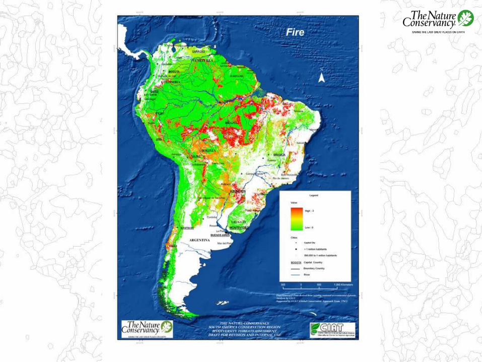
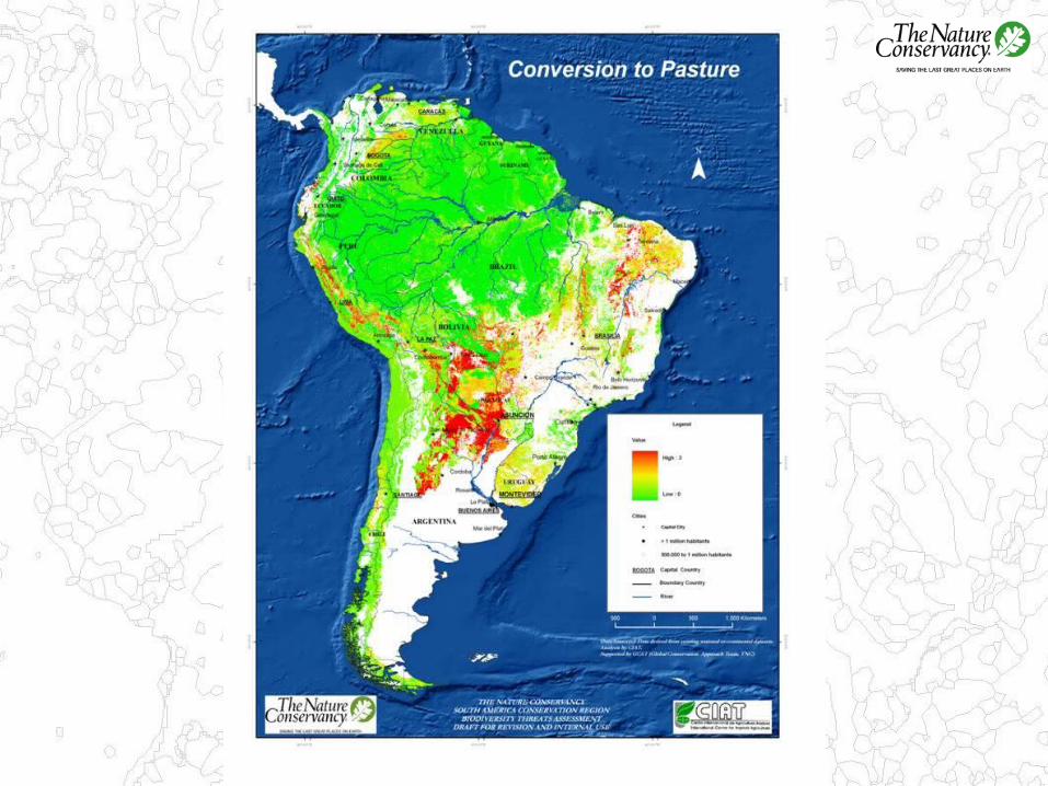
Threats to Biodiversity
• Conversion to pasture• Conversion to agriculture• Infrastructure• Invasive species• Conversion by forestry activities• Fire (in ecosystems without fire regimes)• Pollution• Mining• Oil and gas exploration
Accessibility
• Calculate km/hr to cross 1km cells of roads, rivers, railroads, borders, landcover (glc2000), urban areas (nightlights)
• Merge above and represent the time in minutes
• Factor in elevation, slope
• Divide by 60 to convert to hours, then by 1000 to convert meters to km
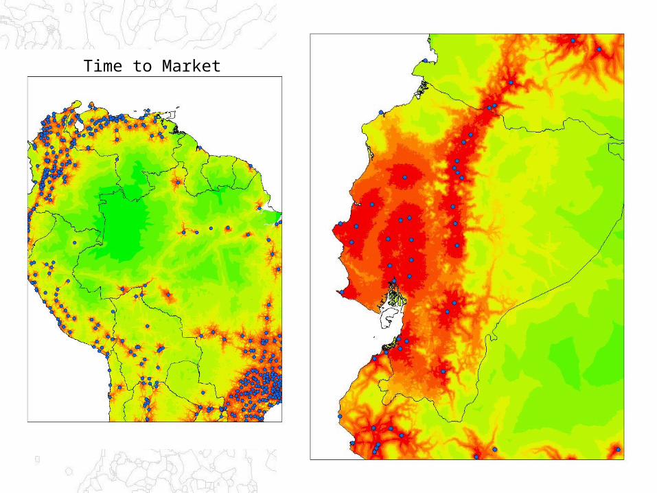
Time to Market
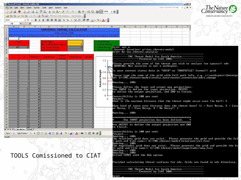
TOOLS Comissioned to CIAT


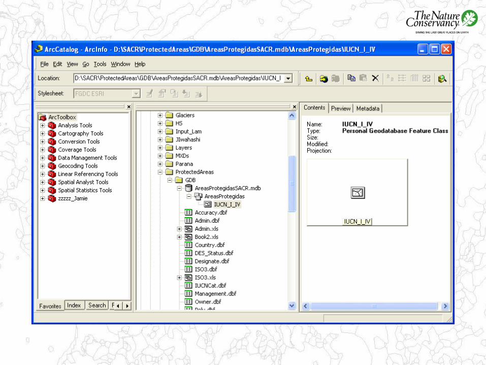
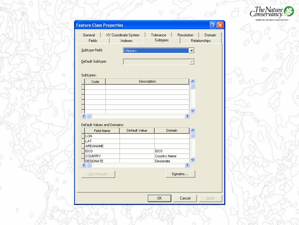
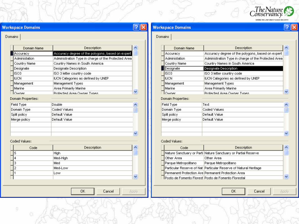
Protected Areas
Data Collection using WDPA as the Standard and improving the
database
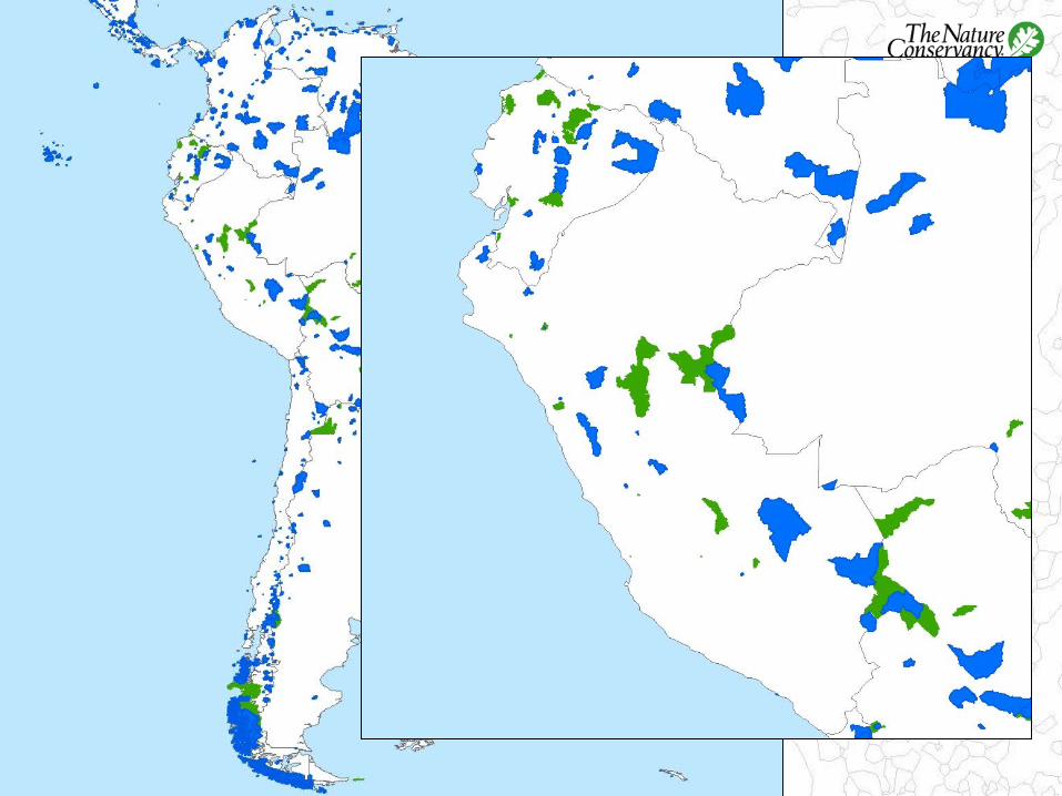
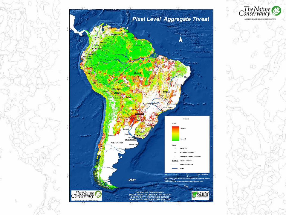
Effective Conservation
• We use the Protected Areas information, Biodiversity information and Threats Analysis
• Estimating how well conservation is doing as a measure
• Monitor conservation efforts
• Find conservation gaps


