Me
Ta
Ub
8
a
A
R
R
2
A
A
K
G
A
M
T
A
P
W
1
T
v
f
f
o
C
t
a
t
i
c
bh0
Process Safety and Environmental Protection 1 1 1 ( 2 0 1 7 ) 375–387
Contents lists available at ScienceDirect
Process Safety and Environmental Protection
journa l h om ep age: www.elsev ier .com/ locate /ps ep
odeling of gas adsorption by aerosol plumesmitted from industrial sources
ov Elperina, Andrew Fominykha, Itzhak Katrab, Boris Krasovitova,∗
Department of Mechanical Engineering, The Pearlstone Center for Aeronautical Engineering Studies, Ben-Gurionniversity of the Negev, P.O. Box 653, 8410501, IsraelDepartment of Geography and Environmental Development, Ben-Gurion University of the Negev, P.O. Box 653,410501, Israel
r t i c l e i n f o
rticle history:
eceived 6 February 2017
eceived in revised form 21 May
017
ccepted 7 June 2017
vailable online 4 August 2017
eywords:
as adsorption
ir pollutants
ass transfer
urbulent diffusion
erosol particles
M2.5–10
ind velocity measurements
a b s t r a c t
Adsorption of trace atmospheric gases by aerosol particles contributes to the evolution of
concentration distribution of the trace constituents and can affect subsequent chemical
reactions in the atmosphere. We suggest a two dimensional model of adsorption of trace
atmospheric constituents by aerosol particles in air pollution plume emitted from an indus-
trial source. The model is based on an application of theory of turbulent diffusion in the
atmospheric boundary layer (ABL) in conjunction with plume dispersion model and model
of gas adsorption by porous solid particles. The wind velocity profiles used in the simu-
lations were fitted from our data previously obtained in field measurements conducted in
the Northern Negev (Israel) using the experimental wind mast. The developed model allows
analyzing spatial and temporal evolution of adsorbate concentration in the gaseous phase
as well as in the particulate matter. The adsorbate concentration distributions are calcu-
lated for the particulate matter PM2.5–10, which is typical for industrial emissions. Analysis
is performed for different meteorological conditions and atmospheric stability classes. It
is shown that the concentration of gases adsorbed by aerosol plume strongly depends on
the level of atmospheric turbulence. The obtained results are compared with the available
experimental data.
© 2017 Institution of Chemical Engineers. Published by Elsevier B.V. All rights reserved.
1998). Atmospheric trace gases adsorbed by PM10 can be transported to
. Introduction
he Earth’s atmosphere contains a variety of aerosols emitted from
arious natural and anthropogenic sources such as fires, volcanoes,
actory stacks, vehicle emissions etc. Atmospheric measurements per-
ormed during last decades revealed an increase of concentrations
f aerosols and active trace gases in the atmosphere, such as HNO3,
O2, SO2 (see, e.g. Rhind, 2009; Boucher, 2015). These findings point to
he importance of investigation of active trace gas scavenging in the
tmosphere due to gas adsorption by aerosols. Scavenging of active
race gases due to gas adsorption in atmospheric transport modeling
s becoming more significant in view of global warming and climate
hange. Indeed, the rise of atmospheric temperature increases a num-
∗ Corresponding author. Fax: +972 8 6472813.E-mail addresses: [email protected] (T. Elperin), [email protected]
[email protected] (B. Krasovitov).ttp://dx.doi.org/10.1016/j.psep.2017.06.022957-5820/© 2017 Institution of Chemical Engineers. Published by Elsev
ber and intensity of dust storms (see, e.g. Johansen, 2009). Emission of
aerosols also increases due to arid and semi-arid lands expansion and
industrial activity. Some trace atmospheric gases, such as nitric acid,
nitrous oxide, iodine, dimethyl sulfide (DMS) are effectively adsorbed
by atmospheric aerosols including carbon based particulate matter
emitted from industrial sources. Adsorption of trace atmospheric
gases by atmospheric aerosols can lead to appreciable changes in the
atmospheric composition and atmospheric properties. For instance,
HNO3 adsorption by mineral dust and carbon based industrial aerosols
depletes nitrogen oxides precursors of the O3 and decreases ozone con-
centration in the atmosphere (see Umann et al., 2005; Choi and Leu,
c.il (A. Fominykh), [email protected] (I. Katra), [email protected],
the large distances. In particular, gaseous nitric acid (HNO3) can survive
ier B.V. All rights reserved.
376 Process Safety and Environmental Protection 1 1 1 ( 2 0 1 7 ) 375–387
List of symbols
a, b Coefficients depending on stability class anddistance from the emission source (see Eq. (2))
ap Particle radius
Bi = aKg/D(p)g Biot number
c Concentrationcp Specific heat capacitydp Diameter of aerosol particleDg Coefficient of molecular diffusion of active gas
in airD
(p)g Coefficient of diffusion of trace gas in a particle
g Gravitational accelerationH Effective stack height or emission heightHA Henry’s constant of adsorptionhA Height of ABLKii Diagonal components of eddy diffusivityKg Coefficient of mass transferm = HA Ssp Dimensionless Henry’s constant of adsorp-
tionk von Karman constantl Turbulent mixing lengthL Monin–Obukhov lengthQ Pollutant emission rateqz Vertical heat fluxRi Richardson numberRiC Critical gradient Richardson numberSa Rate of gas adsorptionSsp Specific surface area of solid particlet TimeT Absolute ambient air temperatureT0 Temperature at the reference heightu Mean wind velocityu* Friction velocityV Volumex Downwind coordinatey Crosswind coordinatez Vertical coordinatez0 Aerodynamic surface roughness length
Greek symbols˛, Coefficients depending on stability class (see
Eq. (2))� Adiabatic lapse rate� Potential temperature� Coefficient of gas adsorption (see Eq. (5))� Density�y, �z Dispersion parameters� Shear stress at the surface levelϕs Volume fraction of solid phase Concentration of aerosol particles
Subscriptsa AirD Diffusiveg Gass Solid
Superscriptsp Particle
long transport distances since dry and wet deposition rate of PM10 is
much smaller than dry and wet deposition rate of gaseous HNO3 (see,
e.g. Dentener et al., 1996). Consequently, gas adsorption by atmospheric
pollutant aerosols can be responsible for intercontinental transport of
active trace gases in the atmosphere.
Atmospheric aerosols influence global climate directly by scattering
and absorbing solar radiation. They can also act as cloud condensation
nuclei (CCN) and ice nuclei (IN) (see, e.g. Fitzgerald et al., 2015) and
change the reflectivity and lifetime of clouds. Adsorption of active trace
atmospheric gases, such as HNO3 and SO2 by atmospheric aerosols
change the optical properties of aerosols, in particular their scattering
and solar radiation absorption properties and enhances absorption of
solar radiation by aerosol particles. Variation of optical properties of
aerosols changes visibility in the atmosphere (see, e.g. Kokhanovsky,
2008). Aging of atmospheric aerosol particles due to adsorption of NOx
enhances their CCN and IN properties. Adsorption of water vapor by
atmospheric aerosols decreases air humidity even in the absence of
vapor condensation.
As indicated in the report of the International Agency for Research
on Cancer (IARC, 2013) the predominant sources of outdoor air pollu-
tion are transportation, stationary power generation, agricultural and
industrial emissions. For a fixed particle volume fraction small particles
have a larger particle surface area that enhances their chemical action
in the human body, e.g. they can cause fibrosis of the lung (see Zhang
et al., 2012). Small aerosols can also adsorb microbes causing infectious
diseases; they can cause blockage in the lungs and degrade resis-
tance to diseases, harm human health and children’s lung development
(Schwartz et al., 1996; Wilson and Suh, 1997; Pope, 2000; Huang et al.,
2003). Some biological aerosols contain viruses, rickettsia, chlamydia,
bacteria, actinomycetes, fungi, and bryophytes, all of which are related
to human diseases (Kanaani et al., 2008).
Theoretical estimate of the rate of adsorption of active trace gas by
spherical aerosol particle was done by Chamberlain et al. (1960) fol-
lowing the approach suggested by Fuchs (1934) for the evaporation of
small droplets. Inspired by studies of Chamberlain et al. (1960), Megaw
(1965) and Garland (1967), a number of theoretical and experimental
investigations were carried out to determine the rate of gas scaveng-
ing due to gas adsorption by single aerosol particles. Hu et al. (2013)
developed a mathematical model of mass transfer controlled by two
phases during active trace gas adsorption by stagnant homogeneous
spherical porous particle and solved numerically nonstationary equa-
tion of diffusion for the dispersed phase with corresponding initial and
boundary conditions. It was assumed that porous particle was initially
free of active gas and as boundary conditions the authors applied con-
ditions of the absence of sink or source of active gas at a center of
particle and the third order boundary condition at gas-particle inter-
phase. Hu et al. (2013) showed that when Bi/m < 0.1, concentration of
adsorbed gas in a dispersed phase can be assumed uniform and the
problem of active trace gas adsorption by solid porous particle reduces
to the solution of the first-order ordinary differential equation with ini-
tial condition. Theoretical predictions agree with experimental results
for semi-volatile organic compounds adsorption by solid particles. Gas
adsorption by particle having a non-uniform porosity, composed of a
nonporous core and a porous outer shell (see e.g., Rounds and Pankow,
1990), was analyzed by Liu et al. (2013). Kalberer et al. (1999) performed
experimental study of adsorption of nitrogen dioxide gas by ensemble
of carbon aerosol particles in low ppb range, pertinent to tropospheric
NO2 concentrations. The size of aerosol particles in the experiments
was of the same order of magnitude as the mean free path of NO2
molecules in air and the typical particle number density in the exper-
iments was 2 × 106 cm−3. It was shown that gaseous NO2 scavenging
by soot particles is governed by chemisorption reaction which is zero-
order in NO2.
Several studies by Murata et al. (1987) and Noguchi et al. (1988, 1990)
were devoted to detailed experimental investigation of gaseous iodine-
131 scavenging by aerosols having different size. Murata et al. (1987)
investigated I-131 adsorption by small incense stick aerosol particles
having the size only by a factor 2 or 3 exceeding the mean free path of
I-131 molecules in air. Noguchi et al. (1988) investigated I-131 adsorp-
tion by large fly-ash aerosols having a significantly larger size than the
Process Safety and Environmental Protection 1 1 1 ( 2 0 1 7 ) 375–387 377
m
a
t
m
i
s
t
t
r
a
t
m
m
t
p
2
2
IaeospitsGpp
woataPccp
wPocespstdee
ean free path of I-131 molecules in air. In the following paper these
uthors studied iodine adsorption by small aerosol particles having
he size of the same order of magnitude as a mean free path of I-131
olecules in air (see Noguchi et al., 1990). In all the above mentioned
nvestigations the authors developed isotherms of adsorption of atmo-
pheric, fly-ash and incense-stick aerosols for I-131 and investigated
he dependence of adsorbed amount of I-131 by aerosols on the reac-
ion time. It was shown that I-131 adsorption by incense stick aerosol
eaches equilibrium after 2 min while the time of saturation for fly-ash
nd atmospheric aerosols is 3–5 times larger.
In the present study we suggest a two dimensional model of adsorp-
ion of trace atmospheric constituents by carbon based particulate
atter in air pollution plume emitted from industrial source. The
odel is based on the application of theory of turbulent diffusion in
he atmospheric boundary layer (ABL) in conjunction with plume dis-
ersion model and model of gas adsorption by porous solid particles.
. Description of the model
.1. Governing equations
n this section, we describe the model of gas adsorption byerosol particles in air pollution plume. Consider an aerosolmission source such as a factory smoke stack. The originf the coordinate system is placed at the base of the smoketack and x-axis is aligned in the downwind direction. Aerosollume rises from the smokestack, levels off and propagates
n x-axis direction while spreading in y-axis and z-axis direc-ions. We assume that the plume is emitted at the effectivetack height H and that air pollutant dispersion is described byaussian distribution. In this case, the Gaussian plume modelrovides the following concentration distribution of aerosolarticles at any downwind distance (see e.g., De Nevers, 1995):
(x, y, z) = Q
2uH�y�zexp
(− y
2
�2y
) [exp
{− (z − H)2
2�2z
}
+ exp
{− (z + H)2
2�2z
}], (1)
here Q is the pollution emission rate; H is the effective heightf the centerline of the pollutant plume; uH is the wind speedt the point of release; �y and �z are the crosswind and ver-ical dispersion coefficients, correspondingly. The horizontalnd vertical dispersion coefficients, �y and �z, depend on theasquill stability classes named A, B, C, D, E, F and G wherebylass A is the most unstable or the most turbulent class, andlass G is the most stable or the least turbulent class. Thearameters �y and �z are determined as follows:
�y = 103x tan �/2.15 �z = axb, (2)
here x is the distance (in km); � = − ln (x) is one-halfasquil’s ϑ (in degrees); ˛, ˇ, a and b are coefficients dependingn stability class and distance from the emission source andan be obtained from the table of parameters for �y and �z (see.g., Turner, 1994; Beychok, 1994). Gaussian models assume theteady-state atmosphere and large time for transport and dis-ersion of aerosols and gases. Although in the atmosphereuch uniform conditions rarely occur, in spite of these limita-ions the Gaussian model is widely used. This model is welleveloped, includes empirical parameterization and has been
xperimentally validated. In our previous study (see Elperint al., 2016), in order to validate the turbulence parameteriza-tion for our Gaussian pollution dispersion model, includingscavenging from Gaussian air pollution plumes and puffs,we compared the results of numerical calculations with theexperimental data obtained during tracer experiments per-formed by Karlsruhe group (Thomas et al., 1983; Thomasand Nester, 1984). Elperin et al. (2016) showed that despite ofthe scatter in experimental data points (Thomas et al., 1983;Thomas and Nester, 1984), at the distances up to 8 km from thesource the agreement of the model with the experimental datais quite fair. The latter assertion is supported by Scorer (1978,see Chapter 10) who noted that concentration of gaseous pol-lutants in the atmosphere can be measured only with theexperimental error of 100–200%.
Mass transfer of active trace gas (adsorbate) in theatmospheric boundary layer (ABL) can be described byadvection–diffusion equation:
∂cg
∂t+ ui
∂cg
∂xi= − ∂u
′ic′g∂xi
− Sa, i = 1, 2, 3, (3)
where cg is the mean concentration of the active trace gas in
ABL, ui are the components of mean wind velocity, u′ic
′g are
components of turbulent fluxes, Sa is the rate of gas adsorp-tion. Hereafter we adopted the turbulence closure based onthe hypothesis of the gradient transport (K-theory) (Seinfeldand Pandis, 2016):
u′ic
′g = −Kii
∂cg
∂xi, i = 1, 2, 3 , (4)
where Kii are the diagonal components of eddy diffusivity ten-sor. It is assumed that the concentration of active trace gas inthe atmosphere is substantially lower that the concentrationof the carrier gas. Hereafter we assume that (i) vertical motionsof air are inhibited and particles and gases are transportedby advection in a horizontal direction; (ii) the wind is unidi-rectional and (iii) the wind velocity depends on the verticalcoordinate only. The Monin–Obukhov (M–O) theory is in excel-lent agreement with experimental data in the case when thedensity stratification in the atmospheric surface layer (ASL)does not deviate too widely from neutral stratification (seee.g. Chapter 4 in Monin and Yaglom, 1971). At the same time,recent experimental evidence has shown that the above the-ory does not adequately describe the ASL in regimes of strongconvection and strong static stability (Hunt, 1998; Zilitinkevichand Calanca, 2000). Generally speaking, convective ASLsare affected by the near-surface convergence flow patternswhich feed the buoyancy-driven semi-organized updraughts,embracing the entire PBL (Zilitinkevich and Calanca, 2000).Moreover, recent studies showed (e.g. Mahrt, 1999; Mauritsenet al., 2007; Grisogono et al., 2007) that the surface-layer for-mulations based on the M–O theory are often not applicable instatically stable conditions. In our investigation we consideredthe stack height that is typical for the industrial emissionsin the Northern Negev region in Israel (≈ 20 m). However, forthe above reasons we do not confine ourselves to consideringtransport of active gases and particles in the surface layer. Inthe steady state case two-dimensional concentration distribu-tion of diffusive adsorbate in a turbulent flow is governed bythe following advection–diffusion equation:
( )
u∂cg∂x= ∂
∂zK(z)
∂cg
∂z− �()cg. (5)

378 Process Safety and Environmental Protection 1 1 1 ( 2 0 1 7 ) 375–387
Table 1 – Pasquil–Gifford stability classes correlated withRichardson number.
Richardsonnumbera
Atmosphericstability
Pasquill–Giffordstability class
Ri ≥ 0.25 Very stable G0 < Ri < 0.25 Stable E–FRi = 0 Neutral D−0.3 < Ri < 0 Unstable C–BRi ≤ −0.3 Very unstable A
a
ducted in the Northern Negev using an experimental windmast. A 10-m wind mast was equipped with 6 cup anemome-
Table 2 – Pasquil–Gifford stability classes correlated withMonin–Obukhov length.
Monin–Obukhovlengtha (m)
Atmosphericstability
Pasquill–Giffordstability class
L < −20 Unstable C−20 ≤ L ≤ −7 Unstable BL > −7 Very unstable A
Boundary conditions for Eq. (5) read:
∂cg
∂z= 0 at z = 0 (6)
cg = cg,∞ at z = hA (7)
cg(0, z) = cg,∞. (8)
In Eq. (5) the term �()c is the rate of loss of active gas dueto adsorption by aerosol particles and K(z) is vertical diffusioncoefficient; hA is the height of ABL. The coefficient �() in Eq.(5) has a similar meaning as the scavenging coefficient in thecase of wet deposition of soluble gases or aerosol particles byrain (Elperin et al., 2011, 2014, 2016, 2017). For stable boundarylayer (SBL) inside the ABL the coefficient K(z) in Eq. (5) can becalculated using the scheme proposed by Blackadar (1979):
K(z) ={
1.1 (RiC − Ri) l2|�u/�z|RiC Ri ≤ RiC
0.001 Ri > RiC
, (9)
where Ri is the gradient Richardson number; RiC is the criti-cal gradient Richardson number (RiC ≈ 0.25); �z is model layerthickness; l is the turbulent mixing length that is parameter-ized as follows:
l = k · z, z ≤ zm
l = k · zm, z > zm. (10)
In Eq. (10) k = 0.4 is von Karman constant and zm accordingto Blackadar’s scheme (see Blackadar, 1979) is assumed to be200 m. The gradient Richardson number is defined as follows:
Ri = g
T
(∂�/∂z)
(∂u/∂z)2, (11)
where g is gravitational acceleration; T is absolute ambient airtemperature, and � is potential temperature. The formula forthe potential temperature reads:
� = T − ��z, (12)
where � is the adiabatic lapse rate; � ≈ − 10−2 K/m over the dis-tance to the mixing depth. Goossens and Offer (1990) showedthat in the Northern Negev area the depth of the ABL, thatcorresponds to the mixing depth, is of the order of 500–600 m.In this case, the potential temperature � is approximatelyequal to the thermodynamic temperature T within 2% error.In meteorology Richardson number is used for characteriza-tion of degree of stratification of the atmospheric boundarylayer. Correlation of the atmosphere stability classes withRichardson number was investigated in numerous studies(see e.g. Sedefian and Bennett, 1980; Zoumakis and Kelessis,1991; Mohan and Siddiqui, 1998; Schnelle, 2001). In the presentstudy we use the correlation for the stability class with theRichardson number suggested by Schnelle (2001) (see Table 1).An alternative model of turbulent transport in stably strati-fied ABL that is based on turbulence energetics and does not
employ the notion of the critical Richardson number was sug-gested by Zilitinkevich et al. (2013).Schnelle (2001).
In the unstable ABL coefficient K(z) can be expressed asfollows (see Dyer, 1974):
K(z) = ku∗z� (z/L)
. (13)
For our purposes in Eq. (13) we used the generally acceptedsimilarity function � (z/L) of Businger et al. (1971), which is asuitable fit to large quantities of experimental data (see e.g.,Seinfeld and Pandis, 2016):
� (z/L) = (1 − 15z/L)−1/4. (14)
For unstable conditions z/L < 0, where L = − �acpT0u3∗
kgqzis the
Monin–Obukhov length, �a is the ambient air density, T0 is theambient temperature at the reference height, g is gravitationalconstant, and qz is the vertical heat flux. The correlation ofPasquill–Gifford stability classes with Monin–Obukhov lengthbased on Praire Grass databases for 44 experiments is sug-gested by Hanna et al. (1990) and is shown in Table 2.
The mean wind velocity profile for the studied case isrequired for simulating the PM dispersion and concentrationdistribution of active gas after emission of aerosol particlesfrom the stack. In ABL the wind profile can be described bythe semiempirical logarithmic law (see, e.g., Shao, 2008):
u = u∗k
ln(z
z0
). (15)
In Eq. (15) u∗ = √�/�a ∝ � is friction velocity, which is a scaling
parameter proportional to the velocity gradient in boundarylayer flow; � is the shear stress at the surface level and �a is airdensity; � is standard deviation of velocity fluctuations (seee.g., Bagnold, 1941; Shao, 2008; Kok et al., 2012); k is the vonKarman constant; z0 is the aerodynamic surface roughnesslength that is approximately equal 1/30 of the field rough-ness elements height in turbulent flow (see e.g., Bagnold, 1941,Chapter 4). In the Negev area roughness elements’ height(pebbles and shrubs) is of the order of 0.2–0.3 m (Offer andGoossens, 1994). Measurements of wind profiles were con-
a Hanna et al. (1990).

Process Safety and Environmental Protection 1 1 1 ( 2 0 1 7 ) 375–387 379
tgtattv9
2
IacwtstgbgatftUte(t
wagKg(Sopei
c
wg
I
c
Table 3 – Henry’s law constant of adsorption of activegases NO2, HNO3 and I-131 by carbon-based aerosolsand coefficient of molecular diffusion in air Dg attemperature T = 298 K.
Gas NO2 HNO3 I-131
HA [cm] 25a 104c 104d
Dg[cm2/s] 0.14b 0.11b 0.08d
a Kalberer et al. (1999).b Seinfeld & Pandis (2016).c Munoz and Rossi, (2002).d Noguchi et al. (1988).
ers positioned at: 0.68, 1.18, 2.0, 3.36, 5.64 and 9.43 m aboveround level (AGL). The instruments record wind speeds inhe range of 0–50 m/s with the accuracy of ±0.49 m/s and with
time interval of 1 min. The anemometers were calibrated inhe laboratory before the field measurements. The best fit tohe experimental data is determined for the friction (shear)elocity u∗ = 0.27 m/s and the roughness z0 = 1.6 × 10⁻³ m with5% confidence bounds (for details see Katra et al., 2016).
.2. Gas adsorption by PM
n order to evaluate the sink term �()cg in Eq. (5) let us considerdsorption of active atmospheric trace gas from a mixtureontaining inert gas and suspended small porous particleshereby velocity of particles is equal to a gas velocity. Assume
hat particles are distributed uniformly in gas-particle suspen-ion and the volume fraction of solid phase ϕs is constant. Athe initial time t = 0 particles begin to adsorb an active traceas from the atmosphere. The size of particles is supposed toe considerably larger than a free path length of molecules in aaseous phase. The characteristic aspect of gas adsorption bytmospheric aerosols is a very low concentration of an activerace gas in the atmosphere. This allows us to use a linearorm of the isotherm of adsorption for the analysis of massransfer, c
(p)g = mcg or U = HA cg at gas–solid interface, where
is adsorbed amount of active gas. Distribution of concen-ration inside a particle is uniform and time-dependent (see,.g. Hu et al. 2013). Following the approach suggested by Hales2002), time derivative of the radius-average concentration ofhe adsorbed gas in a porous particle reads:
dc(p)g (t)
dt= 1�D
(mcg(t) − c
(p)g (t)
), (16)
here c(p)g is the volume-average concentration of the
dsorbed gas in a particle, cg is concentration of an active traceas in a gaseous phase, a is a particle radius, �D = (ap·m)/(3Kg),
g = Dg/ap, Dg is the coefficient of molecular diffusion of activeas in air, ap is the average radius of the solid particles. In Eq.16) m = HASsp, where HA is the Henry’s constant of adsorption,
sp is the specific surface area of solid particle. Volume fractionf particles is equal to ϕs = nVp, n is the number density of solidarticles and Vp = 4
3a3p is the volume of the particle. For an
nsemble-average concentration field the following equalitys valid:
g(t) = cg0 − ϕsc(p)g (t), (17)
here cg0 is an initial concentration of active trace gas in aaseous phase.
Substituting Eq. (17) into Eq. (16), we obtain:
dc(p)g (t)
dt+ c
(p)g (t)
�D(1 + mϕs) = m
�Dcg0. (18)
f c(p)g (t) = 0 at t = 0, solution of Eq. (18) reads:
[ ( )]
(p)g (t) = mcg01 + mϕs1 − exp − (1 + mϕs)t
�D. (19)
Consequently
cg(t) = cg0
{1 − mϕs
1 + mϕs
[1 − exp
(− (1 + mϕs)t
�D
)]}. (20)
The rate of adsorption is determined by the following equa-tion:
dcg(t)dt
= −�cg(t). (21)
Substituting Eq. (20) into Eq. (21) we obtain the followingexpression for the coefficient �:
� =mϕs�
−1D exp
(− (1+mϕs)t
�D
)1 − mϕs
1+mϕs
[1 − exp
(− (1+mϕs)t
�D
)] . (22)
Eq. (22) implies that in the case when m → ∞, � = mϕs�−1D .
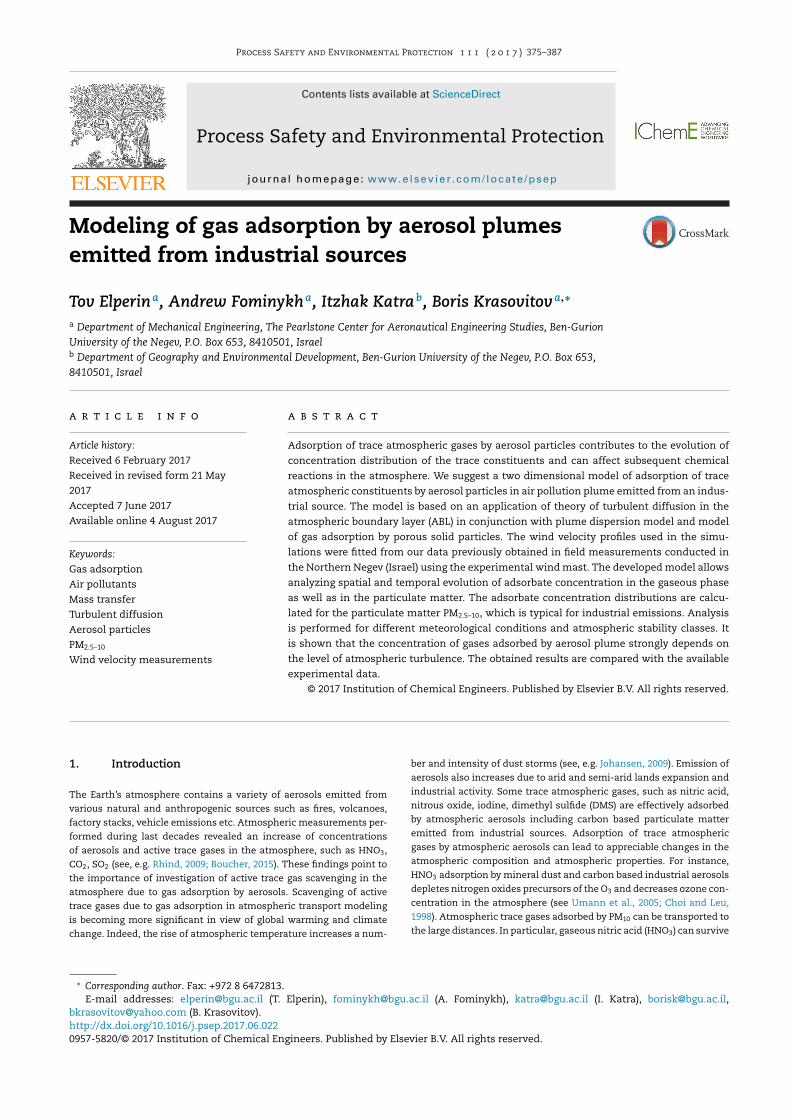
The dependences of the coefficient � vs. time (see Eq. (22))for active gases NO2 and HNO3 and different values of volumefraction of solid phase ϕs are shown in Fig. 1a and b. The valuesof Henry’s law constant of adsorption of active gases NO2 andHNO3 by carbon-based aerosols m and coefficient of moleculardiffusion in air Dg that we have used in our calculations, arepresented in Table 3. Inspection of Fig. 1a and b reveals that thedependence of coefficient � on time is nonlinear and that gasadsorption by gas-particle suspension requires a long time.Furthermore, as can be seen from Fig. 1b, in the case of adsorp-tion of nitric acid HNO3, the time of adsorption is quite large(more than one hour). Therefore, depending on concentrationof the particulate matter, the time of adsorptive scavenging ofvarious trace atmospheric gases varies in the range from a fewminutes to a few hours.
The suggested model of gas adsorption by PM was appliedfor calculation of amount of adsorbed active gas vs. time.Theoretical results were compared with the experimentalmeasurements for iodine gas adsorption by fly-ash aerosolparticles conducted by Noguchi et al. (1988). In the experi-ments of Noguchi et al. (1988) the iodine gas was obtainedby sublimation of a crystal of iodine which was produced byreaction of sodium iodine and potassium dichromate. A dustfeeder generated the fly-ash aerosol in these experiments.Concentration of aerosol particles was measured with con-densation nucleus counter. In the experiments of Noguchiet al. (1988) a mixture of fly-ash aerosol and iodine gaspassed through a cylindrical glass reaction vessel so that par-ticulate iodine could be formed by adsorption of iodine byaerosol. In the experiments, two types of glass vessels hav-
ing volumes 8 l (100 cm length and 10 cm diameter) for a shorttime reaction and 155 l (120 cm length and 45 cm diameter)
380 Process Safety and Environmental Protection 1 1 1 ( 2 0 1 7 ) 375–387
Fig. 1 – Dependence of coefficient � vs. time for the gases:(a) NO ; (b) HNO .
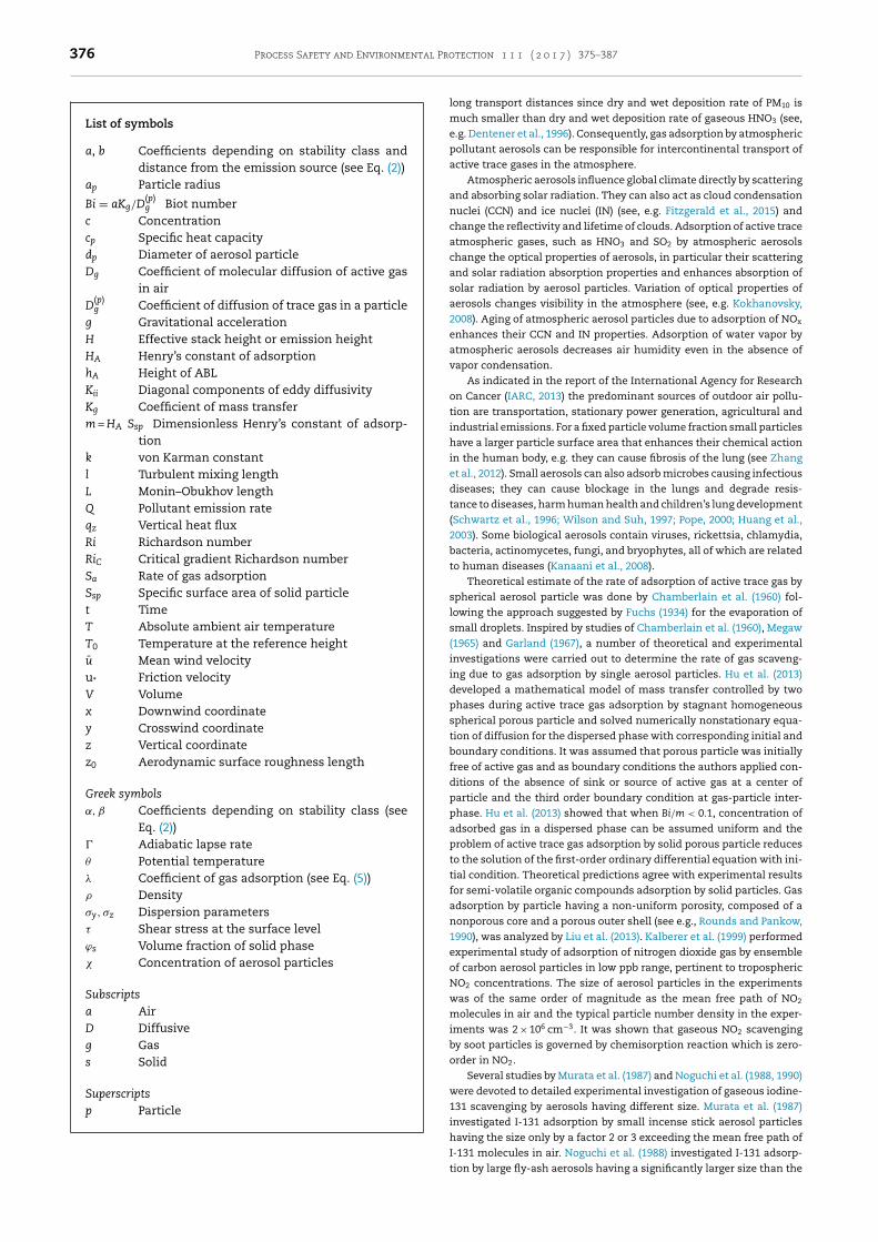
Fig. 2 – Dependence of adsorbed amount of iodine vs. time(cg0 = 1.5 × 10⁻¹⁰ g/cm3, n = 1.02 × 104 cm−3).
2 3
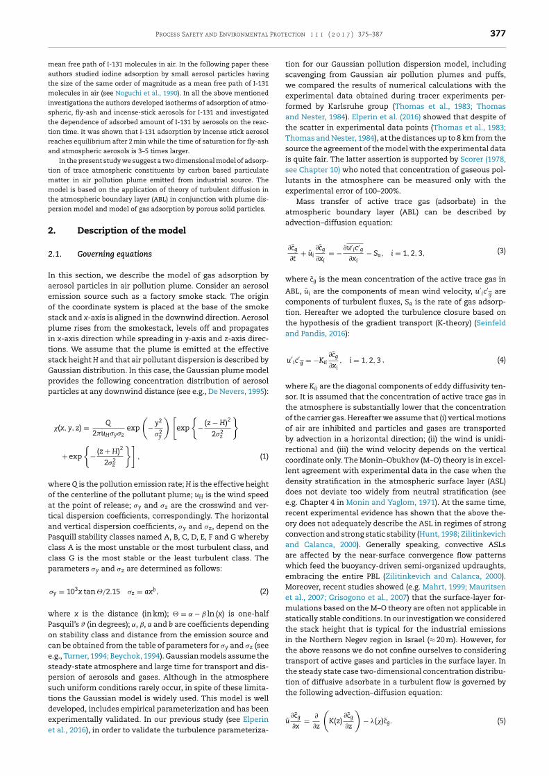
for a long time reaction were used. After the adsorption,the adsorbed particulate iodine and non-adsorbed gaseousiodine were trapped separately using iodine species discrim-inating sampler. The concentration of adsorbed particulateiodine and gaseous iodine was measured with a scintillationcounter. The experiments of Noguchi et al. (1988) were per-formed for cg0 = 5.4 × 10⁻¹⁴ g/cm3 and n = 9, 100 cm−3and forcg0 = 1.5 × 10⁻¹⁰ g/cm3 and n = 10, 200 cm−3 (see Figs. 2 and 3).Average diameter of aerosol particles in experiments wasequal to 0.622 �m. Calculations were performed for specificsurface area of a particles equal to 100 m2 cm−3, typical forcarbon-based aerosols (see, e.g. Kittelson 1998). The effect ofthe specific surface area of particles on the amount of theadsorbed gas is readily apparent from Eq. (19). The larger thevalue of specific surface area of a particle, the larger is theamount of gas that this particle can adsorb (see, e.g. Eq. (19))because the dimensionless Henry’s constant of adsorptionm = HASsp increases with the increase of the specific surface
area of particles. Therefore, the larger is the value of specificsurface area of particles, the more effective is the process ofactive trace gas adsorption by aerosol plume. For very large val-ues of specific surface area of particles and Henry’s constantof adsorption HA the value of the coefficient of gas adsorption� in Eq. (22) is independent of Henry’s constant of adsorptionHA and specific surface area of a particle Ssp.
Results of calculations using Eq. (19) are presented in
Figs. 2 and 3. In Figs. 2 and 3 U = c(p)g S−1
sp , specific surface areaof a particle Ssp = 100 m2 cm−3, density of porous particles wasequal to 1 g cm−3. The value of Henry’s constant of adsorptionfor I-131 was taken from a study of Noguchi et al. (1988) and isequal to 104 cm (see Table 3). Inspection of Figs. 2 and 3 showsthat despite the scatter in experimental data points the agree-ment of the model with the experimental data is quite fair. Theagreement between the experimental results and theoreticalresults presented at Fig. 3 is better than in Fig. 2, because oflesser scattering of experimental results presented in Fig. 3than those in Fig. 2.
Fig. 3 – Dependence of adsorbed amount of iodine vs time(cg0 = 5.4 × 10⁻¹⁴ g/cm3, n = 9.1 × 103 cm−3).

Process Safety and Environmental Protection 1 1 1 ( 2 0 1 7 ) 375–387 381
3
Agcwa
a
�
wabcrN
Fasn
. Numerical simulations
s can be seen from Eq. (5), the term of rate of loss of activeas due to adsorption by aerosol particles �()c depends on theoncentration distribution of aerosol particles at any down-ind distance which is determined by Eq. (1). Taking into
ccount that t = x/u and n = 34�pa3
pEq. (22) can be rewritten
s follows:
=mϕs�
−1D exp
(− (1+mϕs)x
u�D
)1 − mϕs
1+mϕs
[1 − exp
(− (1+mϕs)x
u�D
)] , (23)
here ϕs = /�p and �p is the average particle density. Thedvection–diffusion Eq. (5) supplemented with the initial andoundary conditions (6)–(8) was solved numerically. In theourse of numerical calculations the local coefficient �() was
ecalculated using Eqs. (1) and (23) for the each mesh point.umerical analysis of a gas adsorption by air pollution plumeig. 4 – Distribution of aerosol particles concentration in Gaussiatmosphere calculated in xz-plane at y = 0 (effective stack heighttable atmosphere); (a) distribution of aerosol particles concentraitrogen dioxide NO2; (c) distribution of concentration of nitric ac
described by the advection–diffusion Eq. (5) supplementedwith the initial and boundary conditions (6)–(8) was performedusing MATLAB numerical toolbox.
4. Results and discussion
Using the wind velocity profiles obtained in field measure-ments (Katra et al., 2016) and Eq. (23) for the coefficient �() weperformed numerical analysis of the model of gas adsorptionby aerosol plumes described by the advection–diffusion Eq. (5)supplemented with the initial and boundary conditions (6)–(8).Calculations were performed for the typical industrial emis-sions with the source release rate Q = 10 g/s containing PM2.5–10
particulate matter. The analysis was performed for differ-ent atmospheric conditions categorized by various stabilityclasses. The developed model was applied for the numeri-cal analysis of adsorption of trace atmospheric gases such as
nitrogen dioxide NO2 and nitric acid HNO3 by industrial plumecontaining PM2.5–10 carbon based aerosol particles. It must ben plume and concentration of trace gases in the H = 20 m, source release rate Q = 10 g/s, stability class F —tion in Gaussian plume; (b) distribution of concentration ofid HNO3.

382 Process Safety and Environmental Protection 1 1 1 ( 2 0 1 7 ) 375–387
Fig. 5 – Concentration profiles of atmospheric trace gases inatmosphere calculated in xz-plane at y = 0 (speed of winduH = 6.36 m/s at the height of release, source release rateQ = 10 g/s and effective stack height H = 20 m, Richardsonnumber Ri = 0.2); (a) nitrogen dioxide NO2; (b) nitric acid
noted that the concentration of active gas is much smallerthan concentration of the carrier gas. For instance, the typi-cal AQI (average quality index) for NO2 in the Northern Negevregion in Israel is 41 (≈43 ppb).
Distribution of aerosol particles concentration in Gaussianplume calculated in xz-plane at y = 0 is shown in Fig. 4a. Calcu-lations were performed for the dimensionless concentrationof particulate matter, Cs = uH2/Q , and stable atmosphericconditions (Ri = 0.2) which correspond to the stability class F.
Wind speed uH = 6.36 m/s at the height of release H = 20 mwas calculated using the wind velocity profiles fitted fromdata obtained by Katra et al. (2016) in the field measurementsconducted in the Northern Negev (Israel). Distributions of con-centration of nitric acid HNO3 and nitrogen dioxide NO2 in theatmosphere are shown in Fig. 4b and c. Calculations were per-formed for the relative concentration cg/cg,∞ of active trace gas(where cg is mean local concentration of active gas and cg,∞is the mean concentration of active gas in the atmospherefar from the plume). The values of Henry’s law constant ofadsorption of NO2 and HNO3 by carbon-based aerosols andcoefficient of molecular diffusion in air Dg are given in Table 3for the temperature T = 298 K. As can be seen from these plotsin the inner region near the centerline of the plume HNO3 isalmost fully adsorbed by carbon based aerosol particles whileonly less than 2% of nitrogen dioxide can be adsorbed insidethe plume by aerosol particles emitted from the stack. In thecalculation of concentration distributions of nitric acid HNO3
and nitrogen dioxide NO2 the logarithmic wind profiles fittedfrom data obtained by Katra et al. (2016) were used.
In order to analyze the effect of gas adsorption of tracegases by plume the vertical concentration profiles of NO2 andHNO3 were calculated and shown in Fig. 5a and b. Calcula-tions were performed for the relative concentration cg/cg,∞of active trace gas. The curves in Fig. 5a and b were plot-ted for different distances from the source of release: 25, 50,250 and 500 m and 25, 50, 500 and 2500 m, respectively. Theresults presented in Fig. 5a and b are obtained for Richardsonnumber Ri = 0.2 (stability class F, see Table 1). As can be seenfrom Fig. 5a and b in the stable atmosphere the zone withlow concentration of active gas is located in the vicinity ofthe plume centerline. Moreover, inspection of Figs. 4a and 5ashows that in the case of adsorption of nitrogen dioxide NO2
by aerosol plume the concentration of active gas is a mono-tonically decreasing function of the distance from the source.This is not the case when we consider adsorption of highlyadsorbing gas. In the case of adsorption of nitric acid HNO3
(Fig. 5b), in the near field plume the concentration of active gasalong its centerline decreases with distance from the sourceand then slightly increases while concentration of particulatematter in the plume is a monotonically decreasing function ofthe distance from the source (see Fig. 4a). At the same time,the ground level concentration of active gas decreases withthe distance from the source. The reason is that in the case ofadsorption of highly adsorbing gas such as nitric acid, the con-centration gradient of the active gas near the centerline of theplume is large and the distribution of active gas concentrationstrongly depends on the effect of turbulent diffusion.
In the case of neutral atmospheric conditions (Ri = 0) cor-responding to the stability class D distribution of aerosolparticles concentration in Gaussian plume calculated in xz-plane at y = 0 is shown in Fig. 6a. Calculations were performedfor the dimensionless concentration of particulate matter,
Cs = uH2/Q . The values of height of release, wind of speedat the height of release, source release rate etc. are the sameHNO3.
as in the previous calculations. Distributions of concentrationof nitrogen dioxide NO2 and nitric acid HNO3 in the neutralatmosphere calculated in xz-plane at y = 0 are shown in Fig. 6band c.
As can be seen from these plots in the inner region nearthe centerline the concentration of active gases is lower thanin the exterior region. Furthermore, comparison of Figs. 4b, cand 6b, c shows that in the neutral atmosphere concentrationof active gases in the inner region near the centerline of theplume is higher that in the stable atmosphere.
We also analyzed gas adsorption of nitrogen dioxide andnitric acid by aerosol plume in the unstable atmosphere. In theunstable ABL coefficient of turbulent diffusion K(z) was calcu-lated using Eq. (13) (see Dyer, 1974). Calculations we performed
for the Monin–Obukhov length L = −18 m that is correlatedwith the stability class B (unstable atmosphere). Concentra-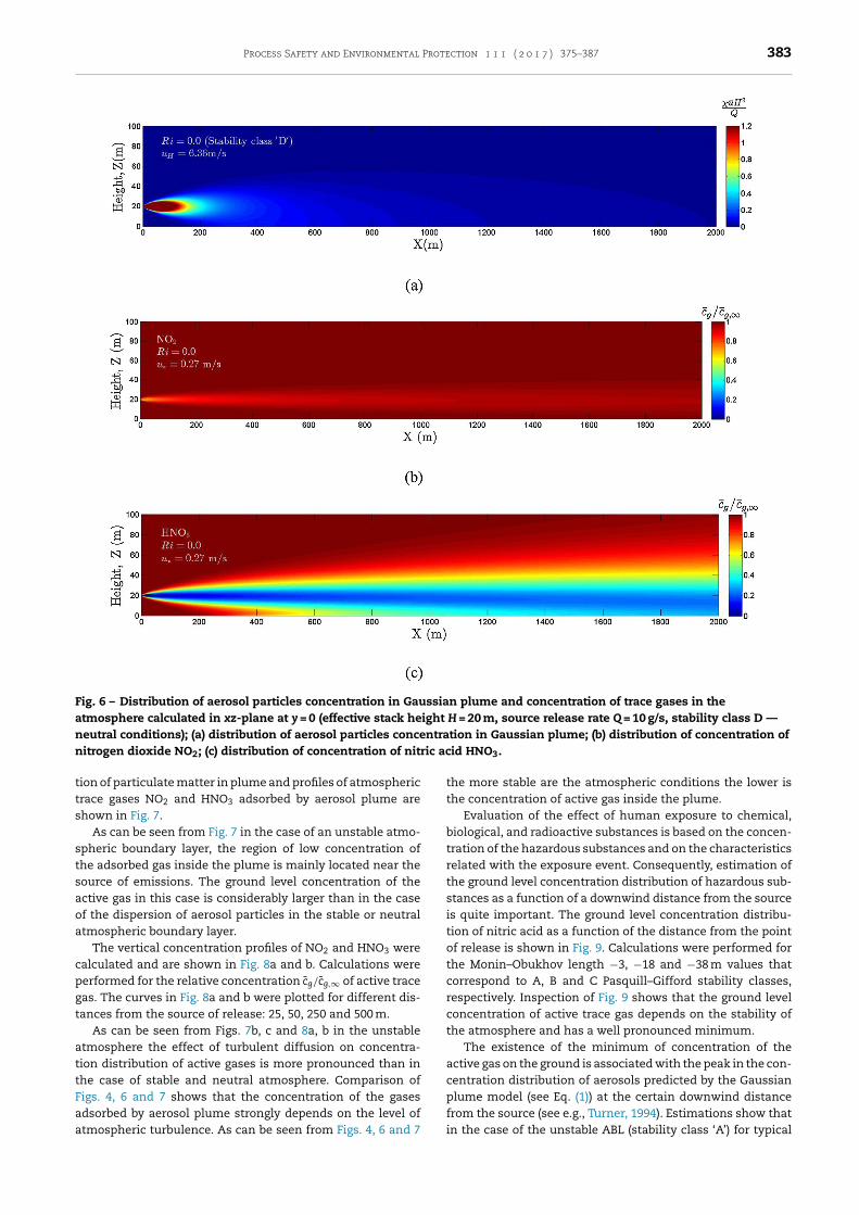
Process Safety and Environmental Protection 1 1 1 ( 2 0 1 7 ) 375–387 383
Fig. 6 – Distribution of aerosol particles concentration in Gaussian plume and concentration of trace gases in theatmosphere calculated in xz-plane at y = 0 (effective stack height H = 20 m, source release rate Q = 10 g/s, stability class D —neutral conditions); (a) distribution of aerosol particles concentration in Gaussian plume; (b) distribution of concentration ofn ric ac
tts
stsaoa
cpgt
attFaa
itrogen dioxide NO2; (c) distribution of concentration of nit
ion of particulate matter in plume and profiles of atmosphericrace gases NO2 and HNO3 adsorbed by aerosol plume arehown in Fig. 7.
As can be seen from Fig. 7 in the case of an unstable atmo-pheric boundary layer, the region of low concentration ofhe adsorbed gas inside the plume is mainly located near theource of emissions. The ground level concentration of thective gas in this case is considerably larger than in the casef the dispersion of aerosol particles in the stable or neutraltmospheric boundary layer.
The vertical concentration profiles of NO2 and HNO3 werealculated and are shown in Fig. 8a and b. Calculations wereerformed for the relative concentration cg/cg,∞ of active traceas. The curves in Fig. 8a and b were plotted for different dis-ances from the source of release: 25, 50, 250 and 500 m.
As can be seen from Figs. 7b, c and 8a, b in the unstabletmosphere the effect of turbulent diffusion on concentra-ion distribution of active gases is more pronounced than inhe case of stable and neutral atmosphere. Comparison ofigs. 4, 6 and 7 shows that the concentration of the gasesdsorbed by aerosol plume strongly depends on the level of
tmospheric turbulence. As can be seen from Figs. 4, 6 and 7id HNO3.
the more stable are the atmospheric conditions the lower isthe concentration of active gas inside the plume.
Evaluation of the effect of human exposure to chemical,biological, and radioactive substances is based on the concen-tration of the hazardous substances and on the characteristicsrelated with the exposure event. Consequently, estimation ofthe ground level concentration distribution of hazardous sub-stances as a function of a downwind distance from the sourceis quite important. The ground level concentration distribu-tion of nitric acid as a function of the distance from the pointof release is shown in Fig. 9. Calculations were performed forthe Monin–Obukhov length −3, −18 and −38 m values thatcorrespond to A, B and C Pasquill–Gifford stability classes,respectively. Inspection of Fig. 9 shows that the ground levelconcentration of active trace gas depends on the stability ofthe atmosphere and has a well pronounced minimum.
The existence of the minimum of concentration of theactive gas on the ground is associated with the peak in the con-centration distribution of aerosols predicted by the Gaussianplume model (see Eq. (1)) at the certain downwind distancefrom the source (see e.g., Turner, 1994). Estimations show that
in the case of the unstable ABL (stability class ‘A’) for typical
384 Process Safety and Environmental Protection 1 1 1 ( 2 0 1 7 ) 375–387
Fig. 7 – Distribution of aerosol particles concentration in Gaussian plume and concentration of trace gases in theatmosphere calculated in xz-plane at y = 0 (effective stack height H = 20 m, source release rate Q = 10 g/s, stability class B —unstable conditions); (a) distribution of aerosol particles concentration in Gaussian plume; (b) distribution of concentration
itric
of nitrogen dioxide NO2; (c) distribution of concentration of nrates of industrial emissions and low wind velocities the dis-tance from the smokestack having the height 20 m where theground concentration of aerosol particles reaches the maxi-mum is of the order of 102 m (Turner, 1994; Elperin et al. 2016).This downwind distance approximately corresponds to thedistance of the minimum of the ground-level concentration ofthe active gas. Such estimations may be useful for the assess-ments of human exposure to gaseous contaminants in theatmosphere and can be used in various air quality models.
5. Conclusions
In this study we suggest a two dimensional model of adsorp-tion of trace atmospheric gases by aerosol particles in airpollution plume emitted from industrial source. The modelis based on an application of theory of turbulent diffusionin the atmospheric boundary layer (ABL) in conjunction withthe plume dispersion model and model of gas adsorptionby porous solid particles. In the calculations the verticalmean wind velocity profiles are fitted from the field measure-ments data conducted in the Northern Negev (Israel) usingthe experimental wind mast (Katra et al., 2016). The adsorbateconcentration distributions are calculated for the particulate
matter PM2.5–10, which is typical for industrial emissions inNorthern Negev (Israel). The analyses of the obtained resultsacid HNO3.
are performed for different meteorological conditions andatmospheric stability classes.
It is demonstrated that spatial evolution of active gas con-centration in the gaseous phase strongly depends on thestability of the atmosphere and efficiency of adsorption ofvarious gases by particulate matter. In particular, it is shownthat in stable and very stable atmosphere the concentra-tion of poorly adsorbing gases such as nitrogen dioxide NO2
monotonically decreases along the plume centerline with thedistance from point of release. In the case of highly adsorbinggases such as nitric acid HNO3 in the near field of the plumethe concentration of active gas along its centerline decreaseswith the distance from the source and then slightly increaseswhile the concentration of particulate matter in the plumedecreases monotonically with the distance from the source.In the case of adsorption of highly adsorbing gas in the sta-ble atmosphere, the concentration gradients of the active gasnear the centerline of the plume are large, and the distributionof active gas concentration strongly depends on the effect ofturbulent diffusion. In the unstable atmosphere the concen-tration distribution patterns for poorly and highly adsorbinggases are similar and differ only by the values of concentra-tion. In the case of the unstable atmosphere we calculated the
ground level concentration distribution of active gases as afunction of the distance from the point of release. It is shown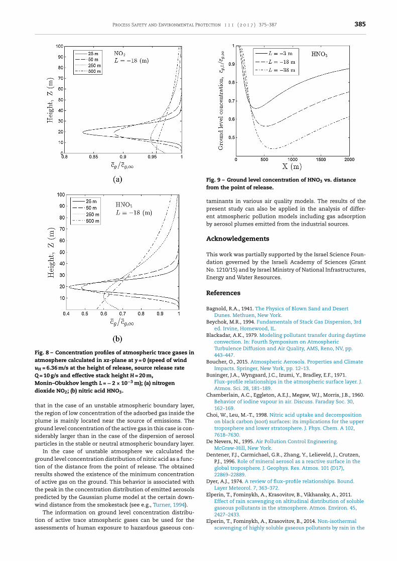
Process Safety and Environmental Protection 1 1 1 ( 2 0 1 7 ) 375–387 385
Fig. 8 – Concentration profiles of atmospheric trace gases inatmosphere calculated in xz-plane at y = 0 (speed of winduH = 6.36 m/s at the height of release, source release rateQ = 10 g/s and effective stack height H = 20 m,Monin–Obukhov length L = − 2 × 10⁻³ m); (a) nitrogend
ttpgsp
gtrotpw
ta
Fig. 9 – Ground level concentration of HNO3 vs. distance
ioxide NO2; (b) nitric acid HNO3.
hat in the case of an unstable atmospheric boundary layer,he region of low concentration of the adsorbed gas inside thelume is mainly located near the source of emissions. Theround level concentration of the active gas in this case is con-iderably larger than in the case of the dispersion of aerosolarticles in the stable or neutral atmospheric boundary layer.
In the case of unstable atmosphere we calculated theround level concentration distribution of nitric acid as a func-ion of the distance from the point of release. The obtainedesults showed the existence of the minimum concentrationf active gas on the ground. This behavior is associated withhe peak in the concentration distribution of emitted aerosolsredicted by the Gaussian plume model at the certain down-ind distance from the smokestack (see e.g., Turner, 1994).
The information on ground level concentration distribu-
ion of active trace atmospheric gases can be used for thessessments of human exposure to hazardous gaseous con-from the point of release.
taminants in various air quality models. The results of thepresent study can also be applied in the analysis of differ-ent atmospheric pollution models including gas adsorptionby aerosol plumes emitted from the industrial sources.
Acknowledgements
This work was partially supported by the Israel Science Foun-dation governed by the Israeli Academy of Sciences (GrantNo. 1210/15) and by Israel Ministry of National Infrastructures,Energy and Water Resources.
References
Bagnold, R.A., 1941. The Physics of Blown Sand and DesertDunes. Methuen, New York.
Beychok, M.R., 1994. Fundamentals of Stack Gas Dispersion, 3rded. Irvine, Homewood, IL.
Blackadar, A.K., 1979. Modeling pollutant transfer during daytimeconvection. In: Fourth Symposium on AtmosphericTurbulence Diffusion and Air Quality, AMS, Reno, NV, pp.443–447.
Boucher, O., 2015. Atmospheric Aerosols. Properties and ClimateImpacts. Springer, New York, pp. 12–13.
Businger, J.A., Wyngaard, J.C., Izumi, Y., Bradley, E.F., 1971.Flux–profile relationships in the atmospheric surface layer. J.Atmos. Sci. 28, 181–189.
Chamberlain, A.C., Eggleton, A.E.J., Megaw, W.J., Morris, J.B., 1960.Behavior of iodine vapour in air. Discuss. Faraday Soc. 30,162–169.
Choi, W., Leu, M.-T., 1998. Nitric acid uptake and decompositionon black carbon (soot) surfaces: its implications for the uppertroposphere and lower stratosphere. J. Phys. Chem. A 102,7618–7630.
De Nevers, N., 1995. Air Pollution Control Engineering.McGraw-Hill, New York.
Dentener, F.J., Carmichael, G.R., Zhang, Y., Lelieveld, J., Crutzen,P.J., 1996. Role of mineral aerosol as a reactive surface in theglobal troposphere. J. Geophys. Res. Atmos. 101 (D17),22869–22889.
Dyer, A.J., 1974. A review of flux–profile relationships. Bound.Layer Meteorol. 7, 363–372.
Elperin, T., Fominykh, A., Krasovitov, B., Vikhansky, A., 2011.Effect of rain scavenging on altitudinal distribution of solublegaseous pollutants in the atmosphere. Atmos. Environ. 45,2427–2433.
Elperin, T., Fominykh, A., Krasovitov, B., 2014. Non-isothermalscavenging of highly soluble gaseous pollutants by rain in the

386 Process Safety and Environmental Protection 1 1 1 ( 2 0 1 7 ) 375–387
atmosphere with non-uniform vertical concentration andtemperature distributions. Meteorol. Atmos. Phys. 125,197–211.
Elperin, T., Fominykh, A., Krasovitov, B., 2016. Effect of raindropsize distribution on scavenging of aerosol particles fromGaussian air pollution plumes and puffs in turbulentatmosphere. Process Saf. Environ. Prot. 102, 303–315.
Elperin, T., Fominykh, A., Krasovitov, B., 2017. Wet precipitationscavenging of soluble atmospheric trace gases due tochemical absorption in inhomogeneous atmosphere.Meteorol. Atmos. Phys. 129, 1–15.
Fitzgerald, E., Ault, A.P., Zauscher, M.D., Mayol-Bracero, O.L.,Prather, K.A., 2015. Comparison of the mixing state oflong-range transported Asian and African mineral dust.Atmos. Environ. 115, 19–25,http://dx.doi.org/10.1016/j.atmosenv.2015.04.031.
Fuchs, N.A., 1934. Concerning the evaporation rate of smalldroplets in gases. Physikalische Zeitschrift der Sowjetunion 6,224–243.
Garland, J.A., 1967. Adsorption of iodine by atmospheric particles.J. Nucl. Energy 21, 687–700.
Goossens, D., Offer, Z., 1990. A wind tunnel simulation and fieldverification of desert dust deposition (Avdat ExperimentalStation, Negev Desert). Sedimentology 37, 7–22.
Grisogono, B., Kraljevic, L., Jericevic, A., 2007. The low-levelkatabatic jet height versus Monin–Obukhov height. Q. J. R.Meteorol. Soc. 133, 2133–2136.
Hales, J.M., 2002. Wet removal of pollutants from Gaussianplumes: basic linear equations and computationalapproaches. J. Appl. Meteorol. 41, 905–918.
Hanna, S.R., Chang, J.S., Strimaitis, D.G., 1990. Uncertainties insource emission rate estimates using dispersion models.Atmos. Environ. 24A (12), 2971–2980.
Hu, K., Chen, Q., Hao, J.H., 2013. Influence of suspended particleson indoor semi-volatile organic compounds emission. Atmos.Environ. 79, 695–704,http://dx.doi.org/10.1016/j.atmosenv.2013.07.010.
Huang, S.L., Hsu, M.K., Chan, C.C., 2003. Effects of submicrometerparticle compositions on cytokine production and lipidperoxidation of human bronchial epithelial cells. Environ.Health Perspect. 111 (4), 478–482.
Hunt, J.C.R., 1998. Eddy dynamics and kinematics of convectiveturbulence. In: Plate, J.E., et al. (Eds.), Buoyant Convection inGeophysical Flows. Kluwer, Boston, MA, USA, NATO ASISeries. Series C, Mathematical and Physical Sciences, 513.
IARC, 2013. In: Straif, K., Cohen, A., Samet, J. (Eds.), Air Pollutionand Cancer. Scientific Publication No. 161. InternationalAgency for Research on Cancer.
Johansen, B.E., 2009. The Encyclopedia of Global WarmingScience and Technology. Greenwood, Santa Barbara, Calif.
Kalberer, M., Ammann, M., Gaggeler, H.W., Baltensperger, U.,1999. Adsorption of on carbon aerosol particles in the low ppbrange. Atmos. Environ. 33, 2815–2822.
Kanaani, H., Hargreaves, M., Ristovski, Z., et al., 2008. Depositionrates of fungal spores in indoor environments, factorseffecting them and comparison with non-biological aerosols.Atmos. Environ. 42 (30), 7141–7154.
Katra, I., Elperin, T., Fominykh, A., Krasovitov, B., Yizhaq, H., 2016.Modeling of particulate matter transport in atmosphericboundary layer following dust emission from source areas.Aeolian Res. 20, 147–156.
Kittelson, D.B., 1998. Engines and nanoparticles: a review. J.Aerosol Sci. 29, 575–588.
Kokhanovsky, A.A., 2008. Aerosol Optics. Light Absorption andScattering by Particles in the Atmosphere. Springer, Berlin,New York, ISBN 978-3-540-23734-1, 153 pp.
Kok, J.F., Parteli, E.J.R., Michaels, T.I., Bou Karam, D., 2012. Thephysics of windblown sand and dust. Rep. Prog. Phys. 75,106901, http://dx.doi.org/10.1088/0034-4885/75/10/106901.
Liu, C., Shi, S., Weschler, C., Zhao, B., Zhang, Y., 2013. Analysis ofthe dynamic interaction between SVOCs and airborne
particles. Aerosol Sci. Technol. 47, 125–136.Mahrt, L., 1999. Stratified atmospheric boundary layers. Bound.Layer Meteorol. 90, 375–396,http://dx.doi.org/10.1023/A:1001765727956.
Mauritsen, T., Svensson, G., Zilitinkevich, S., Esau, I., Enger, L.,Grisogono, B., 2007. A total turbulent energy closure model forneutrally and stably stratified atmospheric boundary layers. J.Atmos. Sci. 64, 4113–4126,http://dx.doi.org/10.1175/2007JAS2294.1.
Megaw, W.J., 1965. The adsorption of iodine on atmosphericparticles. J. Nucl. Energy A/B 19, 555–595.
Mohan, M., Siddiqui, T.A., 1998. Analysis of various schemes forthe estimation of atmospheric stability classification. Atmos.Environ. 32 (21), 3775–3781.
Monin, A.S., Yaglom, A.M., 1971. Statistical Fluid Mechanics, vol.I. MIT Press, Cambridge, MA, USA.
Murata, M., Noguchi, H., Kato, S., Kokuby, M., 1987. Study onadsorption behavior of radioiodine gas using incense stickaerosol. Jpn. J. Health Phys. 22, 21–30.
Munoz, M.S.S., Rossi, M.J., 2002. Heterogeneous reactions of withflame soot generated under different combustion conditions.Phys. Chem. Chem. Phys. 4, 5110–5118.
Noguchi, H., Murata, M., Suzuki, K., 1988. Adsorption ofradioactive iodine gas onto fly ash aerosol. Jpn J. Health Phys.23, 19–26.
Noguchi, H., Murata, M., Suzuki, K., 1990. Adsorption ofradioactive iodine gas onto atmospheric aerosol. Jpn. J. HealthPhys. 25, 209–219.
Offer, Z.Y., Goossens, D., 1994. The use of topographic scalemodels in predicting eolian dust erosion in hilly areas: fieldverification of a wind tunnel experiment. Catena 22, 249–263.
Pope III, C.A., 2000. Review: epidemiological basis for particulateair pollution health standards. Aerosol Sci. Technol. 32, 4–14.
Rhind, S.M., 2009. Anthropogenic pollutants: a threat toecosystem sustainability? Philos. Trans. R. Soc. B 364,3391–3401.
Rounds, S.A., Pankow, J., 1990. Application of a radial diffusionmodel to describe gas/particle sorption kinetics. Environ. Sci.Technol. 24, 1378–1386.
Schnelle, K.B., 2001. In: Meyers, R.A. (Ed.), Atmospheric DiffusionModeling, Encyclopedia of Physical Science & Technology,Atmospheric Science. , 3rd ed. Academic Press.
Schwartz, J., Dockery, D.W., Neas, L.M., 1996. Is daily mortalityassociated specially with fine particles? J. Air Waste Manage.Assoc. 46, 927–939.
Sedefian, L., Bennett, E., 1980. A comparison of turbulenceclassification schemes. Atmos. Environ. 14 (7), 741–750.
Scorer, R.S., 1978. Environmental Aerodynamics. Wiley, New York.Seinfeld, J.H., Pandis, S.N., 2016. Atmospheric Chemistry and
Physics: From Air Pollution to Climate Change, 3rd ed. JohnWiley & Sons Inc., Hoboken, New Jersey.
Shao, Y., 2008. Physics and Modelling of Wind Erosion. KluwerAcademic Publishers, Dordrecht.
Thomas, P., Hubschmann, W., Schuttelkopf, H., Vogt, S., 1983.Experimental Determination of the Atmospheric DispersionParameters at the Karlsruhe Nuclear Research Centerfor160 m and 195 m Emission Heights Part 1: Measured Data.KfKReport 3456, pp. 174.
Thomas, P., Nester, K., 1984. Experimental Determination oftheAtmospheric Dispersion Parameters at the KarlsruheNuclearResearch Center for 160 m and 195 m EmissionHeights. Part 2: Evaluation of Measurements. KfK Report 3457,pp. 102.
Turner, D.B., 1994. Workbook of Atmospheric DispersionEstimates: An Introduction to Dispersion Modeling, 2nd ed.Lewis Publishers, London.
Umann, B., Arnold, F., Schaal, C., Hanke, M., Uecker, J., Aufmhoff,H., Balkanski, Y., Van Dingenen, R., 2005. Interaction ofmineral dust with gas phase nitric acid and sulfur dioxideduring the MINATROC II field campaign: first estimate of theuptake coefficient gamma (HNO3) from atmospheric data. J.Geophys. Res. Atmos. 110 (D22), D22306,
http://dx.doi.org/10.1029/2005JD005906.
Process Safety and Environmental Protection 1 1 1 ( 2 0 1 7 ) 375–387 387
W
Z
Z
Richardson number on stability in the surface layer. Bound.Layer Meteorol. 57, 407–414.
ilson, W.E., Suh, H.H., 1997. Fine particles and coarse particles:concentration relationships relevant to epidemiologic studies.J. Air Waste Manage. Assoc. 47, 1238–1249.
hang, R.-J., Ho, K.-F., Shen, Z.-X., 2012. The role of aerosol inclimate change, the environment, and human health. Atmos.Oceanic Sci. Lett. 5 (2), 156–161,http://dx.doi.org/10.1080/16742834.2012.11446983.
ilitinkevich, S., Calanca, P., 2000. An extended similarity theory
for the stably stratified atmospheric surface layer. Q. J. R.Meteorol. Soc. 126, 1913–1923.Zilitinkevich, S., Elperin, T., Kleeorin, N., Rogchevskii, I., Esau, I.,2013. A Hierarchy of energy-and flux-budget (EFB) turbulenceclosure models for stably stratified geophysical flows. Bound.Layer Meteorol. 146, 341–373.
Zoumakis, N.M., Kelessis, A.G., 1991. The dependence of the bulk


