Transportation Research Part E 47 (2011) 474–489

Contents lists available at ScienceDirect

Transportation Research Part E

journal homepage: www.elsevier .com/locate / t re

Modal freight transport required for production of US goods and services

Rachael Nealer ⇑, Christopher L. Weber, Chris Hendrickson, H. Scott MatthewsCarnegie Mellon University, 5000 Forbes Ave., Pittsburgh, PA 15213, United States

a r t i c l e i n f o

Article history:Received 28 May 2010Received in revised form 29 September2010Accepted 31 October 2010

Keywords:Freight movementCommodity flowModal freight transportationSupply chainInput–output analysis

1366-5545/$ - see front matter � 2010 Published bdoi:10.1016/j.tre.2010.11.015

⇑ Corresponding author. Address: 5000 Forbes AvE-mail address: rnealer@gmail.com (R. Nealer).

a b s t r a c t

In this paper we develop a model which approximates the upstream supply chains forembodied transportation in products. The sector with the largest embodied freight trans-portation in consumption is petroleum products followed by government services, con-struction, and food products. Overall, pipeline contributes 7% to the total embodiedfreight movement per sector, air transport is generally under 1%, water is 5%, and railand truck transportation are the most dominant modes (14% each) for domestic freighttransportation for the average sector. International water is the largest mode (60%) evencompared to domestic modes, and international air contributes less than 1%.

� 2010 Published by Elsevier Ltd.

1. Introduction

Transportation is ubiquitous in the supply chain of goods and services, in the shipment of intermediate inputs, as well asin the delivery of final goods. For example, in the case of automobiles, glass is shipped to windshield manufacturers, wind-shields are shipped to auto manufacturers, and autos are shipped to dealers where consumers buy them. Knowing theembodied transportation needed for the manufacturing and distribution of each product is useful when considering issuessuch as fuel cost changes, traffic congestion, and resiliency and security of the various modes of transportation (Smith et al.,2005). Over the past decades, supply chains and the logistics networks supporting them have become more global, faster,more complex, and more important in the US economy (US DOT, 2010; Meixell and Gargeya, 2005). Broad-scale develop-ments in information and communications technology (ICT) and micro-scale management of businesses (such as just-in-time manufacturing) have increased the visibility and importance of logistics in the world economy (Womack et al.,1990; Klassen, 2000). At the same time, growing awareness of environmental issues such as climate change and air qualityhas made it more important that these increasingly intensive activities are performed in a sustainable way. Since transpor-tation contributes to 33% of US CO2 emissions and large portions of several criteria air pollutants (58% of NOX, 36% of VOCs,and 77% of CO), it is clearly important in efforts to promote environmental sustainability and green supply chain manage-ment (US EPA, 2004; Sheu et al., 2004). Transportation also represents a major investment of public funds, with over $45billion invested in transportation infrastructure by the federal government in 2006 and a comparable amount by stateand local agencies (CBO, 2007).

Understanding the preferred methods of transportation, amounts of commodities shipped, and kinds of commoditiesshipped can provide insight into the resiliency of the transportation system and project future infrastructure improvementsnecessary to create more reliable and efficient methods of transportation. International transportation of both goods andpeople deserves particular mention. International freight transportation to the US (in ton-km) was approximately equal

y Elsevier Ltd.

e., 115 Porter Hall, Pittsburgh, PA 15213, United States. Tel.: +1 412 268 2940; fax: +1 412 268 781.

R. Nealer et al. / Transportation Research Part E 47 (2011) 474–489 475

to total domestic freight ton-km in 2002, as globalization of production increased traffic considerably. The impacts of this areimportant as well, e.g., the emissions associated with international transport are not currently linked to products or coveredby global climate laws (Peters and Hertwich, 2008; Sanchez, 2009; Weber and Matthews, 2008).

It is particularly important to understand the direct and indirect impacts of freight transportation because the totalembodied transportation is likely to be much larger than the direct transportation of a given final product. Decision-makersmay thus underestimate the importance or impacts of transportation to their products. Understanding potential modal vul-nerabilities (e.g., strikes, infrastructure failure) and the response to increasing fuel prices can be useful for managing the riskassociated with transportation. Furthermore, future policies and means to improve efficiency of transportation can be mod-eled at the national level with this research. In this work, we develop a model which approximates the upstream supplychains for embodied transportation in products. We estimate direct, first tier, indirect, and total freight transport require-ments by mode for production in each of 428 interconnected US economic sectors. Here we define ‘‘direct’’ transportationto represent the final delivery of the purchased good to a final consumer. Since service sectors do not produce physical goods,direct transportation would be zero for all service sectors. Service sectors account for approximately 100 sectors out of thetotal 428. First tier transportation represents transportation associated with a sector’s direct inputs from its suppliers. Indi-rect transportation is transportation required in the upstream supply chain. Total, or embodied, transportation is the amountof transportation required to produce a final product or service, and is the sum of direct and indirect transportation for asingle product or service. For example, the direct transportation requirements of an assembled automobile includes deliveryto the sales lot whereas total embodied transportation would include movement of the inputs needed at the assembly line(e.g., the windshield, tires, etc.), transportation to produce these parts from raw materials, transport of raw ores and mate-rials from mines, etc.

Using input–output analysis (IOA), we estimate ‘‘total embodied ton-kilometers’’ across the supply chain of products,similar to past work that has estimated total embodied energy use or emissions across the supply chain for various products(Facanha and Horvath, 2006; Weber and Matthews, 2008). Additionally, this model will quickly estimate direct andupstream transportation estimates for individual economic sectors, which can be further disaggregated into transportationrequired for the final products each sector produces. The model will be available on the Internet at www.eiolca.net fortransportation and sustainability researchers who wish to pursue their own inquiries.

This paper first discusses the model development, including a discussion of the data sources used and their correspondinguncertainties. The two allocation methods used to estimate the direct and indirect transportation for the economic sectorsare detailed in Section 2. The final results are sensitive to the allocation method and show the sectors with the most embod-ied transportation. Section 3 displays the results of the model. Sections 4 and 5 conclude the paper with a brief discussion ofthe results, conclusion, and motivation for future work.

2. Methods and data

There are many studies that quantify the impacts of the direct transportation used to transport US products (Chapman,2007; Corbett and Winebrake, 2007; Vanek and Morlok, 1998). However there are few studies that include the supply chaintransportation embodied in products and services (Facanha and Horvath, 2006). Given the importance of transportation dueto environmental and infrastructure issues, and the growing importance of freight transportation, economic and environ-mental researchers have long tried to understand the interdependence of the productive sectors of an economy and the sup-porting transportation sectors (Leontief and Strout, 1963; Matthews et al., 2001; Williams and Tagami, 2003; Wilson, 1970).Two useful methods for such analyses are input–output analysis (IOA), an economic framework for modeling economy-widesectoral interactions, and life-cycle assessment (LCA), an engineering framework for analyzing the total cradle-to-graveeffects associated with processes, goods and services (Curran, 1996; Horowitz and Planting, 2006; Leontief, 1970; Vigonet al., 1993). The IOA methodology has been used in several studies to determine the embodied transportation in foodproducts, embodied water, and embodied discharge pollution for various US products (Blackhurst et al., 2009; Lave et al.,1995; Weber and Matthews, 2008). Weber and Matthews (2008) is fundamentally similar to the work done for this model,however here we consider the transportation requirements for all US products, not just embodied transportation in foodproducts consumed by households. We further refine the model by evaluating the importance of allocation methods. Thispaper focuses on the development of transportation-focused IOA methods that may later improve tools to assess the lifecycle energy and environmental impacts of produced goods.

The input–output analysis (IOA) framework, first developed by Leontief (Leontief, 1970), is the core of the model. Thetotal output of an economy, represented by vector x, can be expressed as the sum of intermediate consumption, Ax, and finaldemand, y:

x ¼ Axþ y ð1Þ

The square matrix of 428 by 428, A, is the economy’s direct requirements matrix with columns representing the fraction ofinputs purchased from other economic sectors for each of the 428 sectors and the rows representing the IO sectors. Whensolved for total output, x, this equation yields:

x ¼ ðI � AÞ�1y ð2Þ

where the inverted (I � A) matrix represents the so-called Leontief inverse (Miller and Blair, 1985).

476 R. Nealer et al. / Transportation Research Part E 47 (2011) 474–489

The transportation requirements matrix, Dm, shows the direct modal transportation requirements j to produce the eco-nomic output from sector i. The physical meaning of Dm is the transportation purchased to transport a sector’s final goodto any other sector. The seven modes modeled here are air, water, truck, rail, pipeline, international air and internationalwater. The matrix Dm is multiplied by the inverse of the diagonalized vector of the individual sector output inverses, x, toproduce a 428 by 7 final matrix in ton-km per dollar Fm:

Fm ¼ DmdiagðxÞ�1 ð3Þ

This ton-km estimate per sector by mode is transposed and multiplied by the Leontief inverse to estimate the total (directand indirect) embodied transportation by mode (Tm) for each sector for an arbitrary final demand, y:

Tm ¼ F 0mðI � AÞ�1y ð4Þ

The two matrices Fm and Tm can be used to estimate direct and total (direct plus indirect) transportation for production ofparticular goods and services (represented by y). For example, the automobile manufacturing (AM) sector has direct trans-portation of FAM multiplied by the inverse of xAM, where xAM is the automobile manufacturing output. Given the interactionsbetween sectors in the A matrix, we know that for every dollar of output of the automobile manufacturing sector there areinputs from the tire manufacturing sector, the glass manufacturing sector, the steel manufacturing sector, etc. These specificinputs, along with all other supply chain inputs, are calculated using the Leontief inverse.

We also estimate what we refer to as the total embodied transportation in the economy (TETE) of all goods and services,when y represents the entire 2002 US demand for each sector, totaling trillions of dollars.

To populate the data of the transportation flow input–output model, the purely economic requirements need to be linkedwith other information. In the case of this model, data on the transportation requirements of each sector are needed. To cre-ate an estimate of ton-km used for each of the 428 US economic sectors, we created a bridge between commodities made bythose sectors and freight transportation estimates. Future work may link ton-km estimates with data on energy and envi-ronmental effects from burning fuels in vehicles.

The direct requirements matrix, A, is acquired from the Bureau of Economic Analysis data of the 2002 US economy. The2002 Benchmark Input–Output tables are prepared by the Bureau of Economic Analysis and also based on the EconomicCensus. The IO tables summarize interacting economic input and output of industrial sectors and the requirements neededfrom the sectors to make commodities (BEA, 2009). These data are organized using the North American IndustryClassification System (NAICS) which organizes industries by similar processes. At the most detailed level the IO tables aredisaggregated into 428 sectors.

The 428 by 7 matrix Dm is the allocated Commodity Flow Survey freight data. The Commodity Flow Survey (CFS) data areprovided by a partnership between the US Census Bureau, US Department of Commerce, Bureau of Transportation Statistics,and the US Department of Transportation (BTS, 2009). CFS data are organized via Standard Classification of TransportedGoods (SCTG) codes. At the most disaggregated level of detail there are 284 sectors. The most valuable information forour model were data on ton-miles moved, which were converted into units of ton-km (1 ton-km = 0.621 ton-miles).

The total output vector, x, and the total consumption demand vector, y, are both derived from the BEA 2002 Benchmark IOtables. The vector x is used in Eq. (3) to normalize the freight data by sector and mode. The y vector is used in Eq. (4) to cal-culate the final embodied transportation of all US products and services.

Unfortunately, the 2002 CFS and 2002 Benchmark IO tables are not presented at the same level of detail or with the samecommodity or industry classifications. As a result, we developed two methods of allocating the SCTG freight data to appro-priate economic sectors. Overall, there are many ways to allocate commodities to economic sectors and vice versa. The firstmethod used allocates the freight transport data from the reported 284 CFS (SCTG) categories to the 428 IO commodity sec-tors using an assumed mapping bridge, but introduces uncertainty due to the level of data aggregation in the CFS. The secondallocation method uses values of transport services purchased for each economic sector (from the BEA use table) multipliedby an assumed average ton-km per dollar estimate for each mode. Both methods produce individual and often similar esti-mates of ton-km per sector, and are used as min–max estimates for uncertainty analysis. For each allocation method, thetotal amount of freight transportation allocated is validated to ensure it sums to the total ton-km data provided by the2002 CFS. The process for each allocation method is described in Sections 2.1 and 2.2, respectively, and in Appendix A. Thereare also two other difficulties with the CFS data: the lack of any international data and inadequate pipeline data. To supple-ment the CFS data we use other data sources as discussed in Sections 2.3 and 2.4.

2.1. Estimates of transportation requirements via mapping allocation of CFS

The first allocation method allocates CFS sectors into IO sectors using an assumed mapping bridge and creates the directfreight transportation matrix (Dm). The CFS surveys companies for domestic freight movement of their final product com-modities by single or multiple modes, organized by SCTG code. SCTG codes are presented at three levels of detail: two-digit,three-digit, and four-digit. For example, the SCTG ‘‘other agricultural products’’ (two-digit) is disaggregated into fruit, soyabeans, oil seeds, bulbs, live flowers, and fresh-cut flowers (three-digit), and even more disaggregated to fresh fruit, driedfruit, vegetables, soya beans, oil seeds, bulbs, live flowers, fresh-cut flowers, raw tobacco, raw cotton, and other (four-digit).For the purposes of this paper only the three-digit and four-digit data were used. Important sectors, such as coal, are evident

R. Nealer et al. / Transportation Research Part E 47 (2011) 474–489 477

at all levels of detail. The three-digit level of detail is broken down into 133 sectors by transportation mode. At the four-digitlevel there are 284 sectors but, unlike the three-digit level, CFS only reports the total ton-km and is not disaggregated bymode due to data restriction and confidentiality issues. For our estimates, we assumed the total modal breakdown at thethree-digit SCTG level also applies to the corresponding four-digit level total freight data under the three-digit SCTG.

The CFS commodities at the four-digit level generally correspond to commodity sectors in the 2002 Benchmark IO tables,but some assumptions were needed to map the data from CFS to the IO sectors. Since official mapping is not available theSCTG and NAICS sector descriptions were used to develop this concordance. There are three ways the CFS data maps into theIO sectors: multiple CFS sectors map to a single IO sector; a single CFS sector maps to multiple IO sectors; or a single CFSsector maps into a single IO sector. The difficulty in the mapping process occurs when multiple CFS sectors are allocated intoa single IO sector. In this scenario we used an economic allocation taken from the IO detailed item output table (provided byBEA). A detailed example can be found in Appendix A of this paper (see Table 7).

Another necessary allocation was to represent the multiple mode transportation data given in the detailed CFS as singlemode transportation to make the freight data similar to the IO data. The CFS data collection allows companies to report theiruse of transportation by single or multiple modes. Multiple mode commodity shipments in CFS have little detail about themass or distance shipped. For example, CFS summarizes there are 45 billion ton-km in the multiple mode ‘‘truck and water’’,but only 30 billion ton-km are disaggregated due to withheld data or because too much sampling variability prevented it tobe reported. We assumed the total 45 billion ton-km should be allocated to water, since water has more withheld valuescompared to the other modes. Table 1 shows the assumed concordances for all multiple modes. While this introduces uncer-tainty in individual commodity modal shares, it is offset by the fact that the multiple modes represent only 5% of total CFSton-km data. In reality, the data are likely reported by respondents for only the dominant single mode while some companieschoose to report the multiple modes.

2.2. Estimates of transportation requirements via economic allocation of CFS

The second allocation method maps the CFS sectors to IO sectors using an economic allocation. The BEA provides the 2002Benchmark Use table, which shows purchases used for the production of commodities. The columns of the Use table showhow much in goods or services (including transportation) in dollars each sector purchases. The economic allocation methoduses data from the Benchmark IO Use table on transportation services in dollars and multiplies by a constant ‘‘ton-kilometerper dollar’’ to estimate ton-km. The ‘‘ton-kilometer per dollar’’ cost estimate is found by dividing the total ton-km per modeof the CFS data by the total expenditure on each mode from the 2002 Benchmark IO table (BEA, 2009). Table 2 summarizesthe ton-km per dollar estimation process by mode which was verified using public BTS data on freight revenue per ton-mile(BTS, 2003). The total CFS ton-km row is the normalized freight data (Fm) for each mode as estimated by summing CFS dataover all commodities, whereas the total IO expenditure row is the output in dollars found in the IO use table.

Table 2 shows the similar magnitude of domestic truck and rail in terms of ton-km. The most money is spent on trucktransportation, but it is second to air as the most expensive mode to transport goods, with water being the least expensive.It is expected that air, the most expensive, is also the least used when transporting goods, and can explain the large differ-ence between the CFS estimated $/ton-km and the BTS estimate for air. The largest difference is in truck transportation and islikely explained because the BTS estimate includes common carriers.

2.3. International transport

A significant amount of the embodied supply chain of products consumed in the US occurs outside the US. However, sincethe CFS has no data on transport outside of the US, we use additional data sources to estimate international air and water

Table 1Multiple mode to single mode allocation.

Multiple mode Allocated to single mode

Truck and rail RailRail and water WaterTruck and water WaterParcel Truck

Table 2Summary of domestic freight transportation data used for economic allocation by mode.

Mode Air Rail Truck Water

Total CFS ton-km (million) 9390 2,100,000 2,050,000 692,000Total IO expenditure (million $) 9940 36,800 174,000 4080Average estimated $/ton-km 1.1 0.018 0.083 0.0059BTS freight revenue per ton-km 0.48 0.014 0.17 0.0045

478 R. Nealer et al. / Transportation Research Part E 47 (2011) 474–489

transportation by sector. This estimated international transport has been previously documented by Weber and Matthews(Weber and Matthews, 2008). Import statistics of mass by vessel and air, port of entry, and trading partner from the US Cen-sus (US Census, 2005) were combined with estimates of air travel distance (great circle distances between airports) andwater travel distance (along shipping lanes) (NIMA, 2001, 2002) to obtain estimates of ton-km of freight transported forthe imported share of the domestic supply of each sector (Weber and Matthews, 2008). The international travel by airand water to the port of entry (airport or water port) was assumed to represent the entirety of international transport intothe country, and domestic transport averages from CFS were assumed to apply from the port of entry. For products producedin other countries and imported to the US, the transportation embodied in the product would be the same as if it had beenmade in the US. For example, the transportation required for a computer made in China is assumed to be the same as if itwere produced in the US. The international transportation between China and the US in then added in the internationaltransportation vector. The US customs coded import statistics were mapped to IO economic sectors using an existing bridgedeveloped by BEA (2002). These values were normalized by total domestic output in dollars similar to the domestic ton-kmvalues. This method makes the inherent assumption that the share of imports in all domestic purchases is constant. Forexample, purchases of refined petroleum by all sectors are assumed to have the same national average share of importedrefined petroleum and thus the same split of domestic and international transport necessary to supply it.

2.4. Pipeline transportation

Both the CFS and IO data underestimate the freight transported by pipeline. CFS notes that its data does not include crudeoil shipments, a commodity within the oil and gas extraction sector that is mostly transported by pipeline (BTS, 2009). The IOdata cannot be converted to freight movement from the transportation costs in the same method as the other modes becausethe CFS data lacks pipeline freight estimates. Therefore, pipeline freight movement was estimated based on 2002 data fromthe National Transportation Statistics (NTS) (BTS, 2006). Similarly, NTS estimates for natural gas transported by pipelinewere used in place of CFS data. The natural gas point estimate is placed in the natural gas distribution sector (#221200)and the oil point estimate is placed in the oil refineries sector (#324110). It is assumed that all other sectors buy refinedpetroleum, not crude oil, and all refined petroleum requires the input of crude oil. Even though the pipeline estimates aresupplemented by the NTS data, freight data in the petroleum refineries and natural gas sectors also contain movement byother modes. CFS data was used for the non-pipeline freight movement estimates for those sectors. Since only one datasource is used for the pipeline estimates there is no simulation or uncertainty modeled for the pipeline transportationestimates.

2.5. Normalization and simulation

Once domestic and international data were combined and adjusted for pipeline transportation, they were normalized bydomestic commodity output (Eq. (3)). A uniform distribution was assumed between the two allocation method estimates forthe domestic transportation requirements of each sector. Uniform distributions were chosen since there is no detailed infor-mation known about the two estimates or the distribution that defines them. Thus, the two estimates using the mapping andeconomic allocation methods were used as boundaries in which a random sample was selected between them for each sectorby mode. 1000 iterations were simulated, though even at 100 iterations the values begin to converge. Eq. (3) and a MonteCarlo simulation is used to estimate the normalized CFS freight data (Fm) using both mapping and economic allocation meth-ods as boundary values, resulting in Fm transportation matrix in ton-km/$ by sector.

TETE is estimated via Eq. (4) for 1000 iterations to determine the output distribution of total transportation requirementsby sector and mode. The final embodied transportation ton-km estimation matrix is 428 � 7 � 1000, with 428 sectors, 7modes, and 1000 iterations. The results are analyzed and documented in Sections 3 and 4 of this paper.

3. Results

We first present the results of the two allocation methods then follow with simulation results. The CFS data mappingmethod and the economic method produce two distinct estimates of ton-km transported by IO commodity sector and mode.

Fig. 1 shows the distributions of freight movement by mode and allocation method. The values of the normalized CFSfreight data (Fm) are sorted and plotted against the quantity of sectors for each mode. The y-axis is the allocated freightin millions of ton-km. The x-axis is the number of sectors that have freight allocated and continues to the 428th sector,but for visualization purposes only the top 10 sectors are shown. For further visual clarity, the higher values on the y-axisare also truncated, and some values are not shown. Internatonal water has many sectors with large freight requirements,whereas pipeline has large values in only two sectors due to the small number of goods transported by this mode.1 The largevalues for international water movement are skewed by water transportation of oil and gas products. Truck and water ton-kmare close in magnitude, but truck has a few large values, and water has many small values. Air has only a few non-zero values

1 Other goods are transported by pipeline, such as water and wastewater. We only model the transportation of oil and natural gas because they contribute tothe supply chain of the production of goods within the US. Water is also in the supply chain of goods (see Blackhurst et al., 2009).

Fig. 1. Sorted magnitude of direct freight transportation ton-km data (in millions) by sector for two allocation methods.

Table 3Absolute value of difference between allocation methods and corresponding statistics by mode.

Air Rail Truck Water

Number of non-zero sectors 301 313 312 297Mean (ton-km/$) 0.0060 0.83 0.77 0.60% Change in meana 207 �49 6 25Std. Dev. (ton-km/$) 0.043 2.9 2.2 4.4Coeff. of variation 7.2 3.5 2.9 7.290th% (ton-km/$) 0.0055 1.6 1.5 0.6350th% (ton-km/$) 0.0010 0.29 0.25 0.01310th% (ton-km/$) 0.00016 0.10 0.015 0.00035

a Average percentage difference of the economic allocation from the commodity flow survey mapping allocation.

R. Nealer et al. / Transportation Research Part E 47 (2011) 474–489 479

and they are small, similar to international air. The total area under each curve is equal to the total direct transportation of eachmode in millions of ton-km.

A comparison of the normalized allocated estimates (Fm) is shown in Table 3. This table shows statistics of the absolutedifference between the CFS mapping and economic allocation estimates of ton-km per dollar. These estimates demonstratehow sensitive the model is to the choice of allocation method. These values represent the absolute value of the differencebetween the estimation methods for each sector by mode. The international transport and pipeline differences are equalto zero (and not shown) since only one estimation method was used for these modes due to limited data availability.

The number of non-zero sectors are those sectors in which the two allocation methods (mapping and economic) differ intheir estimations of direct freight transportation. There are many service sectors (approximately 100) that do not requiretransportation by either allocation method, so the number of non-zero sectors is important when comparing air and waterto truck and rail, since air and water have fewer non-zero sectors than rail and truck. The robustness of the estimations arequalified by the more non-zero sectors available, and the fewer non-zero sectors show more data are available for that mode.The mean and standard deviation are often lower than the individual allocation methods, however this is not always thecase. Nonetheless, the fact that the differences between the two allocation methods are so large illustrates the considerableuncertainties for estimating the direct movement of goods as well as the total embodied ton-km moved by any individualdetailed input–output sector. The lowest coefficients of variation (COV), in rail and truck, suggest that for these modes thetwo allocation methods predict similar ton-km per dollar estimates for each sector. The two methods have similar truckmean estimates (6% difference) and the economic method underestimates rail by almost half (�49%).The percent changein the mean represents how much the mapping and economic allocation methods differ.

480 R. Nealer et al. / Transportation Research Part E 47 (2011) 474–489

Next we discuss the results aggregated into 28 broad categories to simplify visual comparison as shown in Table 4 (Huanget al., 2009).

Fig. 2 shows the results of the allocated CFS freight data (Dm) aggregated into the 28 sectors of Table 4. The stacked barsshow the average values of Dm by mode for each allocation method. The error bars represent the high and low of the twoallocation methods. The aggregate ‘‘mining’’ group requires about 5.4 billion ton-km of freight transportation to deliverits products, such as coal, oil, and ores. About half of this amount is moved by international water transportation (mostlydue to the transport of imported petroleum). Only one other aggregated group (refined petroleum and basic chemicals)has direct freight movement above 1 billion ton-km. Fig. 2 shows the high dependence of international water, domestic railand truck shipping across many sectors. It also shows that despite the differences in the allocation methods described above,in general the data agree fairly well, especially in sectors with large transportation requirement.

Note that given the data sources to create the model, the ton-km directly demanded by service sectors to deliver productsare zero. This makes intuitive sense because service sectors produce virtual goods; therefore no delivery transportation isrequired for these products. These estimates include only freight transport, not that of customers or employees, whichwas separately estimated by Huang et al. (2009).

Fig. 2 generally shows very little air and pipeline transportation across sectors, and large amounts of truck and water(domestic and international) transportation. The portion of rail or truck transport by sector depends mostly on the valueof the sector’s output—sectors with higher value such as food, chemicals, and apparel tend to be moved by truck. For inter-national freight movement there is no uncertainty since there is only one point estimate for each international estimate,which is why in Table 3 the absolute value of the difference between the sectors is equal to zero for all the statistics.Fig. 3 shows the TETE results by mode for the aggregated 28 sectors.

The sector with the largest embodied freight transportation in consumption is final petroleum products (e.g. gasoline, die-sel, asphalt, etc.) followed by government services, construction, food products, vehicle manufacturing and utilities. This isreasonable when considering what people usually consume and use in large volumes: gas, food, utilities, vehicles, and con-structed public infrastructure. The error bars represent the combined modal 5th and 95th percentiles of the one thousandsimulation iterations for each sector.

Pipeline transport is much more present in each sector compared to Fig. 2 showing that oil and natural gas (the only prod-ucts in the model transported by pipeline) are significant contributors to the upstream activities associated with every sec-tor. Rail transport has also become more present than was shown in the direct transportation for similar reasons—itsdominant commodities moved, mining and raw agricultural products are now embedded in the production of electricity(for coal mining) and final goods. Overall, international water transportation has the largest modal share in ton-km, and di-rect transportation accounts for approximately 27% of the total embodied transportation averaged across all sectors. The ser-vice sectors have embodied ton-km values that become very evident and rival the total freight of many manufacturing

Table 4List of 28 aggregate sector labels.

Index Industry Sector abbrv.

1 Agriculture Ag2 Mining Mine3 Power Generation Power4 Construction Const5 Food, Beverage, and Tobacco Food6 Clothes and Shoes App7 Forest Products For8 Petroleum and Basic Chemicals Petro9 Chemical Products and Drugs Chem

10 Plastics and Rubber Plas11 Non-metallic Minerals Min12 Metals Met13 Fabricated Metal F. Met14 Machinery Manufacturing Mach15 Electronics and Electrical Eqmt EE16 Transportation Vehicle and Eqmt Veh17 Other Manufacturing O. Mfg18 Transportation Trarisrj19 Wholesale, Retail, and Warehousing Wh/R20 Financial, Insurance, and Real Estate IFTR21 Professional Services Prof22 Education Edu23 Healthcare and Social Assistance Health24 Entertainment Enter25 Other Services O. Srv26 Non-electric Utilities Util27 Government Gov28 Other Other

Fig. 2. The allocated direct ton-km aggregated into 28 sectors by mode including international movement. Uncertainty bars represent the two estimates,stacks represent average.

R. Nealer et al. / Transportation Research Part E 47 (2011) 474–489 481

sectors; they contribute to approximately 26% of the total embodied ton-km consumed annually, excluding utilities and gov-ernment sectors. It is also interesting to compare Figs. 2 and 3 to see that the many of the sectors that contribute largeamounts of direct transportation often have a small amount of total (Tm) transportation. Take the mining sector as an exam-ple: there are large amounts of heavy mining products being produced and transported (shown in Fig. 2) that are not con-sumed as final products, but rather as inputs to final products (shown in Fig. 3).

The model uncertainty related to each aggregated sector varies significantly. The sector with the most uncertainty is thenon-electric utilities sectors (Util); this is evident in Fig. 3. The education sectors (Edu), mining sectors (Mine), and othermanufacturing sectors (O. Mfg) also have large model uncertainties in proportion to their total embodied transportationconsumed.

The values above can be further disaggregated into the ton-km necessary for different types of final consumption de-mand. The types of consumption within the total final demand are households, fixed investment, exports, and government.Households consume the most embodied transportation at approximately 63% of US total consumption, followed by exports(10%), fixed investment (22%), and government (5%). The service sectors in particular are mostly consumed by householddemand, whereas fixed investment is mostly driven by freight to support the construction sector.

Relating the direct to total by means of a ratio is also relevant to determine which sectors are using higher amounts ofdirect transportation compared to upstream transportation and vice versa.

Fig. 4 is a visual comparison of the direct to total transportation requirement ratio using the direct transportation as esti-mated by Dm and total transportation as estimated by the embodied transportation (TETE). Of the 28 sectors, 16 have bothdirect and total embodied transportation requirements. Some sectors are not available for comparison since they have noassociated direct transportation requirements (such as service sectors). The sectors on the right of the graph require moredirect transportation as a proportion of the total supply chain logistics. Chemical Products and Drugs, Machinery Manufac-turing, and Plastics and Rubbers need the least direct transportation and more total embodied transportation, implying alonger supply chain with relatively small delivery requirements. The other aggregated sectors’ ratios range from 0.2 to

Fig. 3. Total embodied transportation in the US economy (ton-km) aggregated into 28 broad sectors by mode. Uncertainty bars show the 5th and 95thpercentiles of the 1000 simulation iterations.

Fig. 4. Sorted distribution of direct to total embodied transportation of the economy ratio for the 28 aggregated sectors.

482 R. Nealer et al. / Transportation Research Part E 47 (2011) 474–489

0.6, bounded by Non-metallic Minerals, Other Manufacturing, and Agriculture, which collectively have the highest ratios ofdirect transportation to total transportation. These goods tend to be bulkier and have shorter supply chains, thus requiringmore delivery transport than upstream transport.

R. Nealer et al. / Transportation Research Part E 47 (2011) 474–489 483

When analyzing the disaggregated 428 sectors, there are approximately 150 sectors (35% of all sectors) that have positivelog ratios, meaning they use more direct transportation than indirect transportation. The largest outlier is fishing, followedby other leather products, photo equipment manufacturing, vegetable and melon farming, pottery, ceramics, and plumbingfixture manufacturing. There are many sectors that use more direct transportation than indirect transportation. However,when they are aggregated, as shown above, the sector outliers are averaged in with other sectors.

Another relevant result is the percentage share of each mode in the total supply chain ton-km (Tm) per sector. Fig. 5 showsthese results for the aggregated sectors. Even though pipeline is used as a direct method of freight transport by only twosectors, it is a large contributor to the total profile of freight movement per sector reinforcing the assumption that mostsectors buy fuel from the oil and gas sector in the supply chain of producing their own commodities leading to large relativeton-km (especially for service sectors) in pipeline transport. Air transport is under a few percent for every sector (maximum3% for international air in apparel), and rail and truck transportation are the most dominant modes (14% each) for domesticfreight transportation for the average sector. International water is the largest mode of transport overall, with an average of60% per sector, prominently due to petroleum imports in the supply chain of producing goods and services.

To better illustrate how real-world supply chain freight requirements can be estimated in this model, we estimated thetop ten transportation-intense sectors in the supply chain of a $20,000 vehicle in the Automobile Manufacturing sector(#336111) in 2002. Note that this dollar amount is in producer, not purchaser, price basis.

Overall, row 1 of Table 5 illustrates that approximately 25,000 ton-km (35%) of freight movement in the supply chain ofan automobile are required for the final delivery of a vehicle. This delivery movement (Dm) would include delivering thevehicles to sales lots. In this table the upstream movement in ton-km is further disaggregated into the specific needs ofthe sector. For example to make a vehicle the auto manufacturing sector needs vehicle parts from the motor vehicle partsmanufacturing sector (#336300). This movement of parts is approximately 6000 total ton-km (the first tier ton-km). As asecond example, if the iron and steel mills (#331110) sell steel to the motor vehicle parts manufacturing sector, that trans-portation will be a portion of the iron and steel mills total transportation (ton-km) required. Another portion of transporta-tion would be the automobile sector’s direct purchases from the iron and steel mills, shown as 120 ton-km in the first tiercolumn (i.e., for body parts fabricated at the car plant). This first tier transportation required column is the amount of trans-portation required to move all of the direct inputs necessary to make the vehicle.

Of the parts shipped approximately 40% are shipped internationally. Physically, a vehicle weighs approximately 2 tonstherefore the average vehicle travels 13,000 km to the vehicle sales lot. Approximately 25% of the total ton-km value isshipped via international water which may partially explain the large amount of total ton-km associated with this sector.

The top ten sectors needing transportation for the final automobile represent 47% of the upstream ton-km movementassociated with the automobile manufacturing sector, not including the delivery transportation. This example shows the

Fig. 5. Percentage share of each mode for the total embodied transportation for the economy (ton-km) for each sector estimate.

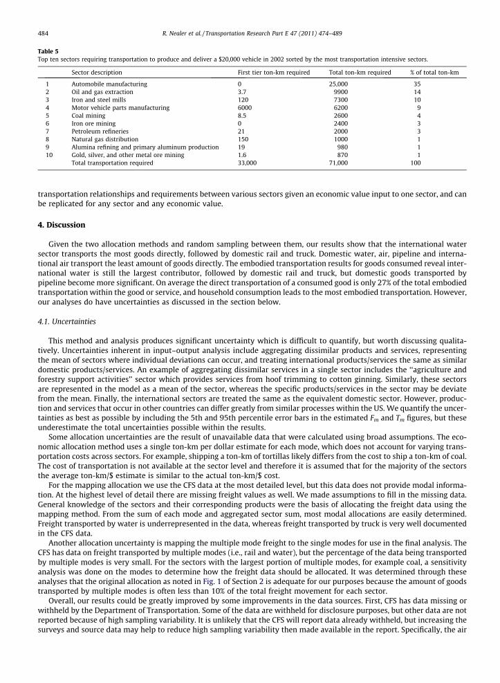
Table 5Top ten sectors requiring transportation to produce and deliver a $20,000 vehicle in 2002 sorted by the most transportation intensive sectors.

Sector description First tier ton-km required Total ton-km required % of total ton-km

1 Automobile manufacturing 0 25,000 352 Oil and gas extraction 3.7 9900 143 Iron and steel mills 120 7300 104 Motor vehicle parts manufacturing 6000 6200 95 Coal mining 8.5 2600 46 Iron ore mining 0 2400 37 Petroleum refineries 21 2000 38 Natural gas distribution 150 1000 19 Alumina refining and primary aluminum production 19 980 110 Gold, silver, and other metal ore mining 1.6 870 1

Total transportation required 33,000 71,000 100

484 R. Nealer et al. / Transportation Research Part E 47 (2011) 474–489

transportation relationships and requirements between various sectors given an economic value input to one sector, and canbe replicated for any sector and any economic value.

4. Discussion

Given the two allocation methods and random sampling between them, our results show that the international watersector transports the most goods directly, followed by domestic rail and truck. Domestic water, air, pipeline and interna-tional air transport the least amount of goods directly. The embodied transportation results for goods consumed reveal inter-national water is still the largest contributor, followed by domestic rail and truck, but domestic goods transported bypipeline become more significant. On average the direct transportation of a consumed good is only 27% of the total embodiedtransportation within the good or service, and household consumption leads to the most embodied transportation. However,our analyses do have uncertainties as discussed in the section below.

4.1. Uncertainties

This method and analysis produces significant uncertainty which is difficult to quantify, but worth discussing qualita-tively. Uncertainties inherent in input–output analysis include aggregating dissimilar products and services, representingthe mean of sectors where individual deviations can occur, and treating international products/services the same as similardomestic products/services. An example of aggregating dissimilar services in a single sector includes the ‘‘agriculture andforestry support activities’’ sector which provides services from hoof trimming to cotton ginning. Similarly, these sectorsare represented in the model as a mean of the sector, whereas the specific products/services in the sector may be deviatefrom the mean. Finally, the international sectors are treated the same as the equivalent domestic sector. However, produc-tion and services that occur in other countries can differ greatly from similar processes within the US. We quantify the uncer-tainties as best as possible by including the 5th and 95th percentile error bars in the estimated Fm and Tm figures, but theseunderestimate the total uncertainties possible within the results.

Some allocation uncertainties are the result of unavailable data that were calculated using broad assumptions. The eco-nomic allocation method uses a single ton-km per dollar estimate for each mode, which does not account for varying trans-portation costs across sectors. For example, shipping a ton-km of tortillas likely differs from the cost to ship a ton-km of coal.The cost of transportation is not available at the sector level and therefore it is assumed that for the majority of the sectorsthe average ton-km/$ estimate is similar to the actual ton-km/$ cost.

For the mapping allocation we use the CFS data at the most detailed level, but this data does not provide modal informa-tion. At the highest level of detail there are missing freight values as well. We made assumptions to fill in the missing data.General knowledge of the sectors and their corresponding products were the basis of allocating the freight data using themapping method. From the sum of each mode and aggregated sector sum, most modal allocations are easily determined.Freight transported by water is underrepresented in the data, whereas freight transported by truck is very well documentedin the CFS data.

Another allocation uncertainty is mapping the multiple mode freight to the single modes for use in the final analysis. TheCFS has data on freight transported by multiple modes (i.e., rail and water), but the percentage of the data being transportedby multiple modes is very small. For the sectors with the largest portion of multiple modes, for example coal, a sensitivityanalysis was done on the modes to determine how the freight data should be allocated. It was determined through theseanalyses that the original allocation as noted in Fig. 1 of Section 2 is adequate for our purposes because the amount of goodstransported by multiple modes is often less than 10% of the total freight movement for each sector.

Overall, our results could be greatly improved by some improvements in the data sources. First, CFS has data missing orwithheld by the Department of Transportation. Some of the data are withheld for disclosure purposes, but other data are notreported because of high sampling variability. It is unlikely that the CFS will report data already withheld, but increasing thesurveys and source data may help to reduce high sampling variability then made available in the report. Specifically, the air

R. Nealer et al. / Transportation Research Part E 47 (2011) 474–489 485

and water transportation have many more missing values than truck and rail. These missing values had to be assumed andcould change the results of the model, although they are not likely to significantly change them because the allocation relieson other CFS data.

Second, the CFS sectors at the most disaggregated level are not described sufficiently to map without uncertainty to the IOsectors. For the freight estimates that did not have a clear CFS to IO sector allocation we assumed that the economic output ofthe sectors as representative of the freight required for that sector. If the results of the CFS were organized similar to the IOsectors or an official mapping was created by the sources it would increase the ease of analyzing the data in terms of freightmovement and economic activity. At the least more detailed descriptions of the sectors in the CFS data at the most aggre-gated level would be a great benefit to future IOA/LCA analyses.

Third, there is no modal data for the most disaggregated level of detail. Additional data on the mode of transportation forthe sectors at the highest level of disaggregation would eliminate the sector specific error associated with how the commod-ities are transported.

Fourth, the CFS has multiple categories of modes that are not consistently reported. There are single modes (i.e., watertransport), detailed single modes (i.e., shallow water transport), and multiple modes (i.e., water and rail transport). Somemodes are represented in one category and some are represented in multiple categories. Furthermore, there are ‘‘unknown’’and ‘‘other multiple’’ modes that are not described in any detail. The inconsistencies, though often small, can be describedand reported with more detail to reduce the uncertainty of the type of transport of the commodities within the correspond-ing sectors.

Lastly, both methods have poor data on pipeline transportation; therefore, the National Transportation Statistics (NTS)published by the Bureau of Transportation Statistics was used. In our model pipeline only affects two sectors: petroleumrefineries and natural gas distribution. Both the CFS data and the BEA data are underestimates of the US pipeline data, withCFS not even accounting for crude oil transportation. Since the transport of gas is withheld in many cases, the NST data arethe most exhaustive data known.

Modeling freight transportation for the US has a significant amount of uncertainty. The CFS and IO data alone have theirown flaws. Specifically, the CFS and IO data are not good at estimating rail and water freight transportation, however, the CFSdoes estimate truck well. Pipeline and international imports are modeled using one data source each, which does not allowthe inclusion of any uncertainty as the other single modes do. This could have a very large effect on the accuracy of the modelbecause the vectors are very large compared to the domestic data. Further information on international transport wouldgreatly improve the accuracy of our model. However, other studies (Weber and Matthews, 2008) show similar transportationratios when comparing 1997 and 2002 direct and total freight transportation for food products. A noticeable difference thatoccurred over the five years is the increased use of international water to transport food products, as well as increasedimports of petroleum and petroleum products in food supply chains.

5. Conclusion

We find that for both the normalized CFS freight data (Fm) and the total embodied transportation (Tm) matrices, interna-tional water transportation is the dominant method of transportation for domestically consumed goods and services,followed by domestic truck and rail. This shows the importance of international trade for the logistics industry and forsupply chains in general. Pipeline transportation is increasingly significant when considering the supply chain of the con-sumption of goods and services. For the total embodied transportation of the economy (TETE) in 2002, the most transportintensive sectors are petroleum products, construction, food, government, vehicle manufacturing, and utilities. Understand-ing these relationships can lead to determining more efficient ways to reduce transportation costs, as well as energy andenvironmental costs economy-wide. Targeting the trucking industry and analyzing the trucking share of each industrymay suggest non-road alternative modes of transportation are sufficient thus reducing traffic congestion on our alreadycrowded roads. Knowing the international transportation shares and the distance goods are shipped can help to identifygoods that may benefit from more domestic production and those where more localized production is feasible. Sectors utilizemodes of transportation differently, and analyzing how they transport their goods could provide insight into the risks asso-ciated with each mode and how to manage it. Similarly, modeling the transportation effects of increasing fuel prices mayyield valuable information on the risks associated with uncertain costs. Additionally, transportation shifts to more efficientmodes as well as increasing mode efficiencies can be modeled per sector and nationally. Sectors with large transportationrequirements can be identified and further explored to find alternatives that reduce costs, energy, and emissions, associatedwith transporting goods. This model could help decision-makers prioritize ways of reducing costs, energy, and emissionswithin the transportation sector while taking the supply chain of disaggregated sectors into account.

This research adds to the literature a supply chain model that estimates the ton-km for each sector in the US economywhich is important in understanding freight movement and modal resiliency. Little research has calculated the embodiedtransportation of products, and this information can be important to decision-makers. Relating this estimated freight move-ment to energy required, greenhouse gas emissions, transportation costs, and time may lead to more effective policies inreducing the freight transportation emissions, create more efficient infrastructure, and minimize risks associated with fuelcosts and infrastructure failure. All these applications can reveal more information about the freight transportation industrythat can bring better and more efficient policies that effect transportation and environmental costs.

Table 6Example allocation when multiple CFS sectors map into a single IO sector.

CFS sector Ton-km (Mil) IO sector Ton-km (Mil)

Soya beans 87,900 Oilseed farming 95,200Oil seeds and nuts, except olives and soya beans 7300

Table 7Example allocation when one CFS sector maps into multiple IO sectors.

CFS Sector Ton-km (Mil) IO Sector Output ($Mil) Allocation (%) Ton-km ($Mil)

Fresh or dried nuts 1180 Tree nut farming 3500 30 360Snack food manufacturing 8000 70 800Sum 11,500

Table 8Applying modal breakdown from three-digit to four-digit CFS data.

Three-digit CFSsector

Mode Three-digit ton-km bymode (Mil)

Percent oftotal (%)

Four-digit CFSsector

Four-digit ton-km (Mil)

ModalBreakdown

Four-digit ton-km bymode (Mil)

Paints Truck 9480 93 Paints 9400 Truck 8700Water S 0.3 Water 28Rail 680 6.7 Rail 630Air 6 0.0006 Air 0.05Total 10,200 Total 9400

Table 9Example economic allocation calculation for Oilseed Farming.

Air Rail Truck Water

Oilseed farming IO Sector Transportation Costs 70 377 588 54Average Estimated Ton-km/$Mil 0.95 57.2 11.78 169.70Estimated Oilseed farming Ton-km (Mil) 67 21,600 6930 9160

486 R. Nealer et al. / Transportation Research Part E 47 (2011) 474–489

Acknowledgements

We would like to thank the National Science Foundation for financial support of this project under Grant number0755672. Any opinions, findings, and conclusions or recommendations expressed in this material are those of the author(s)and do not necessarily reflect the views of the National Science Foundation. They also thank Catherine Izard of Carnegie Mel-lon University for assistance, and the reviewers for their time and comments.

Appendix A. Estimated Ton-km calculation examples

A.1. Mapping CFS freight data to IO sectors

When multiple CFS commodity sectors are mapped to a single IO commodity sector (i.e., because the definition of the IOsector includes both commodities) the calculation is a simple summation of the ton-km of the CFS sectors. An example of thisallocation is the ton-km of the CFS SCTG sector ‘‘Soya beans’’ and ‘‘Oil seeds and nuts, except olives and soya beans’’ whichare mapped to the ton-km of ‘‘Oilseed farming’’ IO sector (#1111A0). Table 8 details the actual calculation.

Additional information is needed to allocate the CFS data to multiple IO sectors. The IO detailed item output use table wasused to economically allocate a portion of the CFS sector to multiple IO sectors within the mapping estimation method (24).Table 8 shows the example of this when mapping the CFS commodity of ‘‘Fresh or dried nuts’’ into the IO sectors of ‘‘Tree nutfarming’’ (#111335) and ‘‘Snack food manufacturing’’ (#311910) since fresh or dried nuts are listed under both industry IOcommodity descriptions. Using the IO detailed item output table we determine that the ‘‘Tree nut farming’’ IO industry sectoraccounts for 30% of the expenditures associated with the ‘‘Fresh or dried nuts’’ IO sector, with the remaining 70% of theexpenditures related to the ‘‘Snack food manufacturing’’ IO sector. We then extrapolate the expenditure percentages tothe ton-km estimates for the final allocation of 3500 ton-km to ‘‘Tree nut farming’’ and 8000 to ‘‘Snack food manufacturing’’(see Table 9).

R. Nealer et al. / Transportation Research Part E 47 (2011) 474–489 487

The last type of allocation of the CFS freight data are related to the modal split of transportation per sector. At the highest,most disaggregated, level of commodity data there is no detail on the mode of transportation. Therefore, the mode percent-ages from the CFS three-digit level are calculated with respect to the total and applying it to the given total ton-km at thefour-digit level. An example calculation is shown in Table 10. This example is for the case where one three-digit sector goesinto two four-digit sector, which is why the totals are not identical, and the remaining 800 ton-km are allocated to the otherpaint and varnish four-digit sector in the same modal proportions shown in Table 10. Generally, multiple four-digit sectorsmake up one three-digit sector in which the percentages derived from the three-digit data will hold throughout each asso-ciated four-digit sector.

A.2. Economic allocation of CFS data

The economic allocation method is the multiplication of the transportation costs per mode derived from the IO use tableand an average estimated ton-km per dollar estimate. The average estimated ton-km per dollar estimate by mode is shownin Table 11 and the calculation to find the estimated ton-km using the IO data for the Oilseed farming sector is displayed inTable 5. Multiplying the transportation costs in $Mil per sector and the average estimated ton-km per $Mil results in an esti-mated ton-km (in millions).

Note that the economic and mapping allocations result in different estimates, however the total ton-km for all sectorssum to the same amount. The difference lies within how the total ton-km are allocated to the individual sectors.

Appendix B. Statistical data on CFS and IO allocation methods

Table 3 shows statistics of the normalized mapping allocation method across all 428 sectors (with sectors equal to zeroremoved from the analysis of each mode). It statistically describes how the data is allocated using the mapping allocationand can be compared to Table 12 with the economic allocation statistics to see how they differ in allocation methods.

The non-zero sectors range from 2 to 308 out of the 428 sectors for pipe and truck, respectively. Truck and rail have thelargest total ton-km per dollar estimates which shows the ubiquity of these modes when not considering upstream supplychain transportation. The coefficient of variation (Std. Dev./Mean) is small for modes with less variation between the sectors.Also note the large standard deviations for each mode compared to the mean showing that within the 428 sectors there is alot of variance in both total modal freight requirements and modal splits. The total values exhibit less variation than modalvalues since different sectors will tend to use different transportation methods given the relative value to weight ratio oftheir products, geographical distribution, and other factors. However, if the top five ton-km per dollar estimates are removedfrom the data the coefficient of variation (COV) decreases by approximately 80% for air, 50% for rail, 20% for truck, and 60% forwater, showing that outliers are significant in this data.

The 10th, 50th (median), and 90th percentiles show the skew of the data distributions. The data with a 90th percentileclose to the median will have a probability distribution function that is skewed to the right. All the modes, with the exceptionof pipeline, show that there are fewer high estimates than low estimates, and all the probability distributions functions arethus skewed right.

Both international water and air are shown separately in Table 4, which shows statistics on the international freightmovement and which do not differ between the allocation methods.

The data underlying Table 4 have more non-zero sectors compared to domestic transport and are similar to the amount ofdata available for the most prevalent sources of domestic freight movement, rail and truck. The largest commodity shippedby international water transport is crude oil, representing 54% of total international ton-km. Similar to the domestic modesof transportation the standard deviation is relatively high compared to the mean, however the coefficient of variation is rea-sonably low. Again the 10th, 50th, and 90th percentiles show a probability distrubition function skewed to the right, in otherwords the low values of ton-km per dollar are more frequent across the sectors.

Table 5 shows that the statistical results are similar for the economically allocated ton-km vector but there is more sectorto sector variability.

Table 10Statistics of CFS mapping allocation for freight transport by input output sector and mode (excluding sectors with zero transport).

Mapping allocation

Air Pipe Rail Truck Water

Number of non-zero sectors 217 2 237 307 285Total (ton-km/$) 1.7 11 165 206 94Mean (ton-km/$) 0.0076 5.5 0.70 0.67 0.33Std. Dev. (ton-km/$) 0.051 0.75 3.5 1.3 2.7Coeff. of variation 6.7 0.14 5.0 2.0 8.190th% (ton-km/$) 0.0070 5.9 1.1 1.5 0.2850th% (ton-km/$) 0.0012 5.5 0.026 0.30 0.01010th% (ton-km/$) 0.00015 5.0 0.0019 0.015 0.00035

Table 11Statistics for international freight transport by IO sector and mode excluding sectors with zero transport.

Intl. Air Intl. Water

Number of non-zero sectors 296 300Mean (ton-km/$) 0.014 1.4Std. Dev. (ton-km/$) 0.041 5.4Coeff. of variation 2.9 3.990th% (ton-km/$) 0.025 2.450th% (ton-km/$) 0.0033 0.2310th% (ton-km/$) 0.00012 0.0073

Table 12Statistics for economic allocation of freight transport by input output sector and mode (excluding sectors with zero transport).

Economic allocation

Air Pipe Rail Truck Water

Number of non-zero sectors 291 2 312 289 158Mean (ton-km/$) 0.0025 5.5 1.4 0.63 0.26Standard deviation (ton-km/$) 0.0030 0.75 12 2.5 0.75Coefficient of variation 1.2 0.14 8.9 3.9 2.890th% (ton-km/$) 0.0049 5.9 1.4 1.2 0.7850th% (ton-km/$) 0.0018 5.5 0.30 0.042 0.04410th% (ton-km/$) 0.00038 5.0 0.13 0.0028 0.0036

488 R. Nealer et al. / Transportation Research Part E 47 (2011) 474–489

The economic allocation has large standard deviations as well as higher coefficient of variation (COV) for air, rail andwater, but lower COV for truck. This demonstrates that the economic method allocates air, rail, and water freight transpor-tation with more variation throughout the sectors compared to the mapping method, it is most likely due to sectors not pay-ing the same value per ton-km. Rail transport has the largest mean estimate, which differs from the mapping allocationmethod. Truck transport has the second largest mean ton-km per dollar estimate. When removing the top five sectors ofthe most ton-km per dollar estimates the COV for air decreases 20%, rail decreases 85% and truck decreases 40%, and waterdecreases 30%. Note that pipeline estimates for each allocation method is the same since they are point estimates taken fromNST. All the modes in the economic allocation method are also skewed to the right, similar to the mapping allocation. Eventhe number of non-zero sectors differs from the mapping allocation, which is further detailed in the Table 6 in the differenceof methods.

References

Bureau of Economic Analysis, 2002. Concordance between 2002 Input–Output Commodity Codes and Foreign Trade Harmonized Codes. <http://bea.gov/industry/io_benchmark.htm#2002data>.

Bureau of Economic Analysis, 2009. 2002 Benchmark Input–Output Accounts. Bureau of Economic Analysis, Department of Commerce. <http://www.bea.gov/industry/io_benchmark.htm>.

Blackhurst, B.M., Hendrickson, C., Vidal, J.S.I., 2009. Direct and indirect water withdrawals for US industrial sectors. Environmental Science & Technology 44(6), 2126–2130.

Bureau of Transportation Statistics, 2003. Table 3-17: Average Freight Revenue per Ton-mile. Bureau of Transportation Statistics. <http://www.bts.gov/publications/national_transportation_statistics/html/table_03_17.html>.

Bureau of Transportation Statistics, 2006. Table Table 1-46b: US Ton-Miles of Freight. Bureau of Transportation Statistics, US Department of Transportation.<http://www.bts.gov/publications/national_transportation_statistics/html/table_01_46b.html>.

Bureau of Transportation Statistics, 2009. Commodity Flow Survey 2002. US Department of Commerce, Services Division, Washington, DC. <http://www.bts.gov/publications/commodity_flow_survey/>.

Congressional Budget Office, 2007. Trends in Public Spending in Transportation and Water Infrastructure, 1956 to 2004. Congress of the United States,Congressional Budget Office.

Chapman, L., 2007. Transport and climate change: a review. Journal of Transport Geography 15, 354–367.Corbett, J., Winebrake, James, 2007. Sustainable movement of goods; energy and environmental implications of trucks, trains, ships, and planes.

Environmental Management, 8–12.Curran, M.A., 1996. Environmental Life-cycle Assessment. McGraw-Hill, New York.Facanha, C., Horvath, A., 2006. Environmental assessment of freight transportation in the US. International Journal of Life-cycle Assessment 11 (4), 229–239.Horowitz, K.A., Planting, M.A., 2006. Concepts and Methods of the US Input–Output Accounts. US Bureau of Economic Analysis, Washington, DC.Huang, Y.A., Weber, C.L., Matthews, H.S., 2009. Categorization of scope 3 emissions for streamlined enterprise carbon footprinting. Environmental Science &

Technology 43 (22), 8509–8515.Klassen, R.D., 2000. Just-in-time manufacturing and pollution prevention generate mutual benefits in the furniture industry. Interfaces 30 (3), 95–106.Lave, L.B., Cobas-Flores, E., Hendrickson, C.T., McMichael, F.C., 1995. Using input–output analysis to estimate economy-wide discharges. Environmental

Science & Technology 29 (9), 420A–426A.Leontief, W., 1970. Environmental repercussions and the economic structure: an input–output approach. The Review of Economics and Statistics 52 (3),

262–271.Leontief, W.W., Strout, A., 1963. Multiregional input–output analysis. In: Barna, T. (Ed.), Structural Interdependence and Economic Development. Macmillan,

London.Matthews, H.S., Hendrickson, C.T., Soh, D.L., 2001. Environmental and economic effects of E-commerce: a case study of book publishing and retail logistics.

Transportation Research Record 1763, 6–12.

R. Nealer et al. / Transportation Research Part E 47 (2011) 474–489 489

Meixell, M.J., Gargeya, V.B., 2005. Global supply chain design: a literature review and critique. Transportation Research Part E: Logistics and TransportationReview 41 (6), 531–550.

Miller, R.E., Blair, P.D., 1985. Input–Output Analysis: Foundations and Extensions, 1 ed. Prentice-Hall, Englewood Cliffs, NJ.National Imagery and Mapping Agency, 2001. Distances between Ports. National Imagery and Mapping Agency.National Imagery and Mapping Agency, 2002. World Airports – DAFIF. National Imagery and Mapping Agency.Peters, G.P., Hertwich, E.G., 2008. CO2 embodied in international trade with implications for global climate policy. Environmental Science and Technology 42

(5), 1401–1407.Sanchez, M., 2009. Email for energy use of current fleet of US computers and computer monitors. In: Weber, C.L. (Ed.), Pittsburgh, PA.Sheu, Jiuh-Biing, Chou, Yi-Hwa, Hu, Chun-Chia, 2004. An integrated logistics operational model for green-supply chain management. Transportation

Research Part E: Logistics and Transportation Review 41 (4), 287–313.Smith, A., et al., 2005. The Validity of Food Miles as an Indicator of Sustainable Development. UK DEFRA, London, pp. 1–117.US Census, 2005. US Imports and Exports of Merchandise Monthly DVD-ROM. US Census Foreign Trade Division, Washington, DC.US Department of Transportation, Research and Innovative Technology Association, Bureau of Transportation Statistics, 2010. Freight Transportation:

Global Highlights, Washington, DC.US Environmental Protection Agency, 2004. National Air Quality and Emissions Trends Report, 2003 Special Studies Edition Office of Air Quality and

Standards, Air Quality Strategies and Standards Division.Vanek, F.M., Morlok, Edward K., 1998. Freight energy use disaggregated by commodity. Transportation Research Record 1641, 3–8.Vigon, B.W., Tolle, D.A., Cornaby, B.W., Latham, H.C., Harrison, C.L., Boguski, T.L., Hunt, R.G., Sellers, J.D., 1993. Life Cycle Assessment: Inventory Guidelines

and Principles. US Environmental Protection Agency, Washington, DC.Weber, C.L., Matthews, H.S., 2008. Food-miles and the relative climate impacts of food choices in the United States. Environmental Science & Technology 42

(10), 3508–3513.Williams, E., Tagami, T., 2003. Energy use in sales and distribution via E-commerce and conventional retail. Journal of Industrial Ecology 6 (2), 99–114.Wilson, A.G., 1970. Interregional commodity flows: entropy maximizing procedures. Geographical Analysis 2, 255–282.Womack, J.P., Jones, D.T., Roos, D., 1990. The Machine that Changed the World. Rawson Associates, New York.

Glossary

Coefficient of variation (COV): The standard deviation divided by the mean yields a normalized measure of the variation of data; the larger the COV the morevariation within the data.

Direct Transportation: Fm; Freight transportation of a final product, not including any consumer transportation.Final Demand: Consumption demand of the US in 2002.First Tier Transportation: Freight transportation of the final product or service and all of its direct inputs.Indirect/Supply Chain Transportation: The transportation associated with all the processes needed to produce a final product or service.Input–output analysis (IOA): An economic framework for modeling economy-wide sectoral interactions.International transportation: The sum of US water and air international exports.Life Cycle Assessment (LCA): An engineering framework for analyzing the total cradle-to-grave environmental pressures associated with processes, goods

and services.Leontief inverse: Commodity-by-commodity form of the direct requirements matrix; mathematically, the inverse of the I matrix minus the requirements

matrix.Monte Carlo simulation: Numerical integration using random selections within set boundaries; used to model implicit uncertainty of the variables.Sectors: Grouped industries similar in production of goods and services that are subgroups the US economy.Ton-kilometer: Unit of measurement for both weight and distance.Total Transportation: fm; Sum of direct and indirect (upstream) transportation.Total Embodied Transportation of the Economy (TETE): Total freight movement necessary to produce goods and services for the demand of the 2002 US

economy.