
MixSIH: a mixture model for single individual haplotyping
Hirotaka Matsumoto , Hisanori Kiryu
Department of Computational Biology
Graduate School of Frontier Sciences
The University of Tokyo

• Introduction
– What is haplotype ?
– What is Single Individual Haplotyping (SIH)?
– An unnoticed problem in SIH (No confidence score)
• Methods
– Probabilistic model for SIH (Simplified version)
– Confidence score based on our model
– Actual model and optimization procedure
• Results
– Dataset
– Comparison of accuracies
– Other analyses
2

Introduction
• Human somatic cells are diploid and contain two homologous copies of chromosomes.
• The two chromosomes differ at a number of loci such as SNP.
3
homologous
A G T T C
A A T T C
SNP

What is haplotype ?
• Haplotype is the combination of alleles on a single chromosome.
• If there are two heterozygous loci, there are two possible haplotypes.
4
---A ATG CT---
---AAATGGCT---
---AGATGTCT--- A G G T
---AAATGTCT---
---AGATGGCT---
? genotype
haplotype
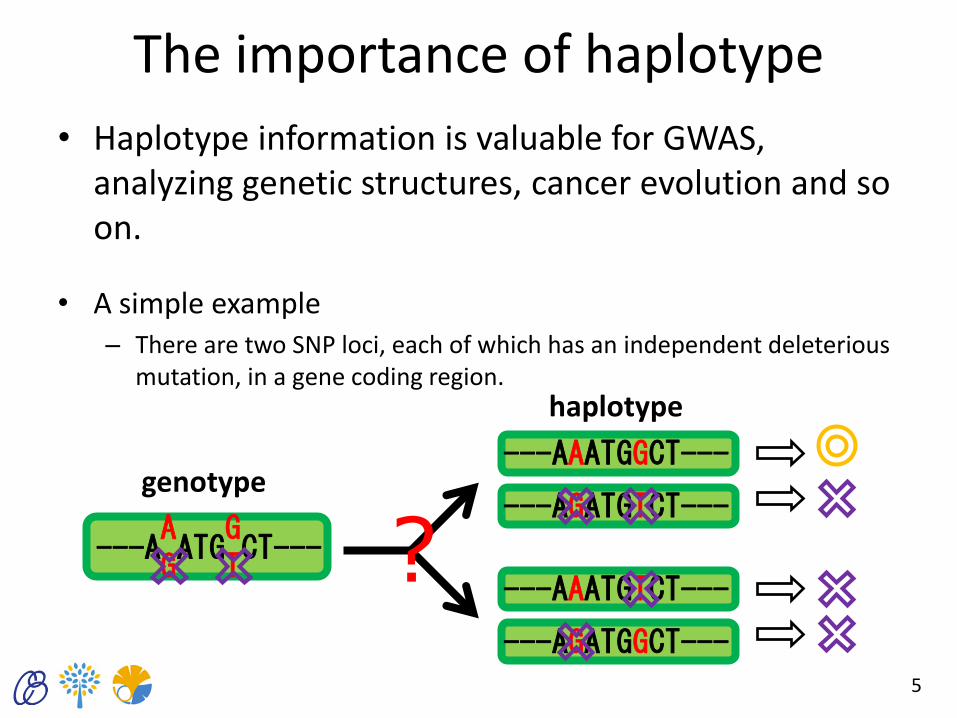
The importance of haplotype
• Haplotype information is valuable for GWAS, analyzing genetic structures, cancer evolution and so on.
• A simple example – There are two SNP loci, each of which has an independent deleterious
mutation, in a gene coding region.
5
---A ATG CT---
---AAATGGCT---
---AGATGTCT--- A G G T
---AAATGTCT---
---AGATGGCT---
? genotype
haplotype

Approaches for haplotype inference
• It is difficult to determine haplotypes experimentally, and there are several computational approaches for haplotype inference.
1. Statistically construct a set of haplotypes from population
genotypes. (statistical haplotype phasing)
2. Reconstruct haplotypes by using genotypes of pedigree.
3. Infer an individual’s haplotypes from sequenced DNA
fragments. (single individual haplotyping (SIH))
6
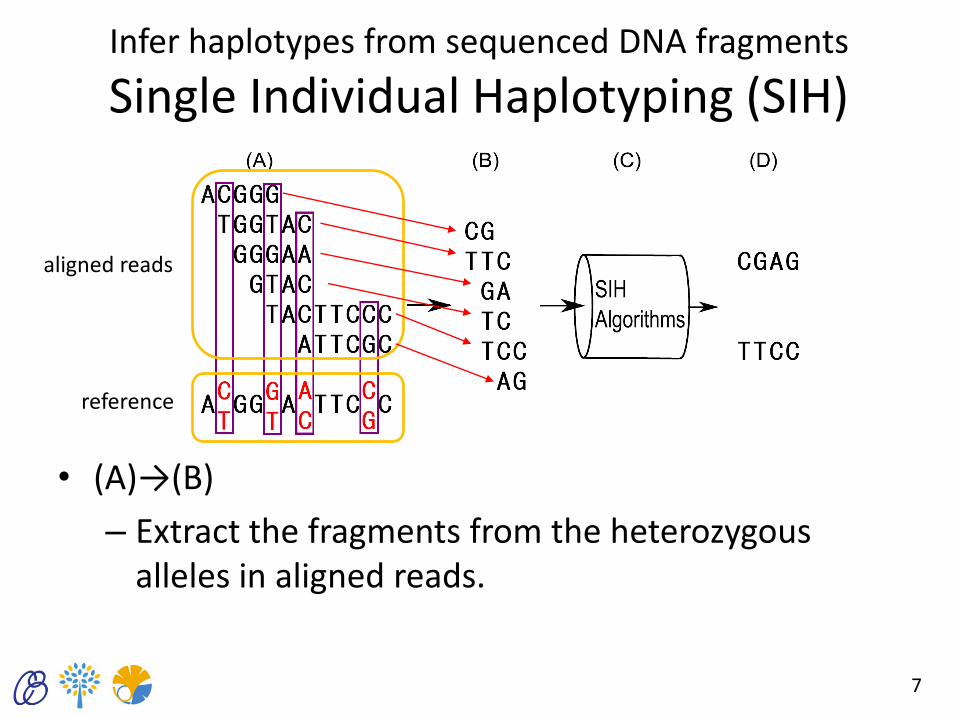
Infer haplotypes from sequenced DNA fragments
Single Individual Haplotyping (SIH)
• (A)→(B)
– Extract the fragments from the heterozygous alleles in aligned reads.
7
aligned reads
reference

Infer haplotypes from sequenced DNA fragments
Single Individual Haplotyping (SIH)
• (B)→(D) (i)
– Co-occurrence of alleles in the same read (intra).
8

Infer haplotypes from sequenced DNA fragments
Single Individual Haplotyping (SIH)
• (B)→(D) (ii)
– Overlap between the reads (inter).
9

The problem and the view of SIH
• SIH uses the reads which span multiple heterozygous loci.
– next-generations sequencing is not long enough
– Sanger sequencing is too expensive
• This situation is changing rapidly with the advent of experimental techniques.
– real-time single molecule sequencing
– fosmid pool-based next generation sequencing
10

Important point in haplotype inference
• The haplotype information which contains errors is likely to lead to wrong results in downstream analyses. – In detecting the recombination events
• To use haplotype information in downstream analyses while avoiding such harmful influence of errors, it is important not only to assemble haplotypes as long as possible but also to provide means to extract highly reliable haplotype regions.
11

The problem of SIH algorithms
• In the statistical haplotype phasing, reliable haplotype regions are determined by selecting the blocks of limited haplotype diversity and level of linkage disequilibrium (LD).
• Although there are many algorithms for SIH, none of these algorithms can provide confidence scores to extract reliable haplotype regions.
• We developed an algorithm which provides the confidence scores of the regions.
12
• Introduction
– What is haplotype ?
– What is Single Individual Haplotyping (SIH)?
– An unnoticed problem in SIH (No confidence score)
• Methods
– Probabilistic model for SIH (Simplified version)
– Confidence score based on our model
– Actual model and optimization procedure
• Results
– Dataset
– Comparison of accuracies
– Other analyses
13

Notation
• We only consider the heterozygous sites and represent them as binary.
• We extract the heterozygous alleles from the DNA sequenced reads and describe these reads as “fragments”.
14
mapped reads
reference
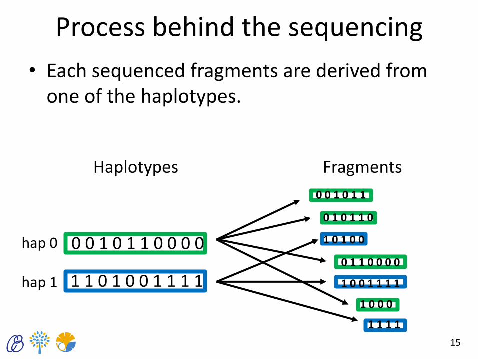
Process behind the sequencing
• Each sequenced fragments are derived from one of the haplotypes.
15
0 0 1 0 1 1 0 0 0 0
1 1 0 1 0 0 1 1 1 1
0 0 1 0 1 1
0 1 0 1 1 0
1 0 1 0 0
0 1 1 0 0 0 0
1 0 0 0
1 0 0 1 1 1 1
1 1 1 1
hap 0
hap 1
Haplotypes Fragments

Observed data
• The contents of the fragments are only observed and haplotype states and the derivation of the fragments are not observed.
16
?
?
0 0 1 0 1 1
0 1 0 1 1 0
0 1 1 0 0 0 0
1 0 1 0 0
1 0 0 0
1 0 0 1 1 1 1 ?
Observed data (input data)
1 1 1 1
hap 0
hap 1
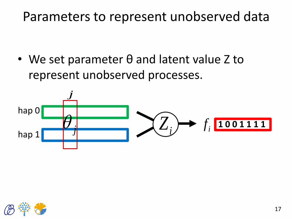
Parameters to represent unobserved data
1 0 0 1 1 1 1 if
17
jhap 0
hap 1
j
iZ
• We set parameter θ and latent value Z to represent unobserved processes.

Parameters to represent unobserved data
1 0 0 1 1 1 1
if if
if
18
jhap 0
hap 1
j
1. Zi is the latent value to represent the derivation of fi
1
0
0
1 orZi
hap 0 hap 1
hap 0 hap 1

Parameters to represent unobserved data
1 0 0 1 1 1 1 if
19
jhap 0
hap 1
j
2. θj is the set of parameters to represent the state of site j
0 1
1 0
a:
j
b:
bj
aj
j
,
,
1,, bjaj

Parameters to represent unobserved data
1 0 0 1 1 1 1 if
20
jhap 0
hap 1
j
The probability is as follows;
Z j
Z
fXk
hfk
Z j
Z
iiii
ji
i
iki
jihfPjhPfP1
0 )(
),(,
1
0
,
,
, 5.0),|()()|(
)|( ifP
if ih 5.0)1()0( ii hPhP
)( ifXk if・ ・
・
b
ahf iki
),( ,
if
if )0,1()1,0(),(
)1,1()0,0(),(
,
,
orhf
orhf
iki
iki
where is the derivation of and
means the site which covers

Parameters optimization and haplotype inference
• Optimizing Z and θ simultaneously is impossible, and we use EM algorithm for optimization.
• The haplotypes of site j is the state whose probability is higher than another.
– If
21
N
i Z j
Z
iii
N
i
ijihfPjhPfPFP
1
1
01
,),|()()|()|(
bjaj ,, 0 1
a: j

Confidence score of a site
22
• The confidence of connection of haplotypes at site j is calculated from the optimized parameter.
where
)|)((
)|)((log
)|(
)|(log)(tyconnectivi
jFP
jFP
FP
FPj
)(,
)(,
,,,,
,,,,
jk
jk
akbkbkak
bkbkakak

Confidence score of a site
23
• This is the illustration of “connectivity”.
)|)((
)|)((log
)|(
)|(log)(tyconnectivi
jFP
jFP
FP
FPj
hap 0
hap 1
hap 0
hap 1 )( jF
)|)(( jFP )|)(( jFP
j

Confidence score of a region
24
)(tyconnectivimin),(MC21
21 jjjjjj
• We extend “connectivity” to the confidence scores of the regions (MC).
• MC is the minimum ”connectivitiy” in the region.
• We tested whether reliable regions could be extracted by using MC values.

Actual model
• Add sequencing error term
• Define the prior distribution and optimize parameter with Variational Bayes EM (VBEM) algorithm.
25
),(,)(
),(,
)(
),(,,,,
)1(),|(),|(iki
i
iki
i
iki hfkfXk
hfkii
fXk
hfkii hfPhfP

Actual parameter optimization
• Iterative twist operations to avoid sub-optimal solutions.
26
)|()|( if FPFP
① ② ③ ④
⑤
① ② ③ ④ ⑤
Do Variational Bayes EM with initial parameter. Select the site which has smallest “connectivity”. Do VBEM with twisted parameter. Compare the probabilities and select better parameter. Iterate from step ② until smallest connectivity over 7.0.

• Introduction
– What is haplotype ?
– What is Single Individual Haplotyping (SIH)?
– An unnoticed problem in SIH (No confidence score)
• Methods
– Probabilistic model for SIH (Simplified version)
– Confidence score based on our model
– Actual model and optimization procedure
• Results
– Dataset
– Comparison of accuracies
– Other analyses
27
Dataset (Simulation data)
• True data
– Generate M binary heterozygous loci randomly.
• Input data
– Replicate each true haplotype c times and randomly divide them into subsequences of length between l1 and l2. Then randomly flipped the binary values of the fragment from 0(1) to 1(0) with probability e.
28

Dataset (Real data)
• Input data
– Duitama’s work who conducted fosmid pool-based NGS for HapMap trio child NA12878 from the CEU population.
• True data
– Haplotypes of about 82% (1.36*10^6/1.65*10^6) sites are determined by trio-based statistical phasing method and are conducted by 1000 Genomes Project.
29

Fosmid pool-based NGS (1)
30
① ②
Genomic DNA is fragmented into pieces of length about 40 kilo-bases and construct fosmid library. Fosmid clones are randomly partitioned into barcoded 32 pools.
① ②

Fosmid pool-based NGS (2)
31
③
Sequencing and mapping. Reads draw a block which corresponds to a fosmid library. Convert a block into a fragment.
③
④
⑤
reference
A C G G
A G A
G A C G G
A G ⑤
④

True data (Trio-based data)
32
A|C|A|G C|G|T|G
A|C|T|G A|G|T|T
A|C|A|G C|G|T|T

True data (Trio-based data)
33
A|C|A|G C|G|T|G
A|C|T|G A|G|T|T
A|C|A|G C|G|T|T
C ? A T A ? T G
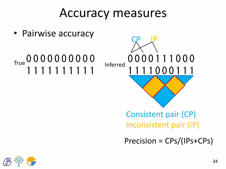
Accuracy measures
• Pairwise accuracy
34
0 0 0 0 0 0 0 0 0 0 1 1 1 1 1 1 1 1 1 1
0 0 0 0 1 1 1 0 0 0 1 1 1 1 0 0 0 1 1 1
True Inferred
Consistent pair (CP) Inconsistent pair (IP)
Precision = CPs/(IPs+CPs)
CP IP
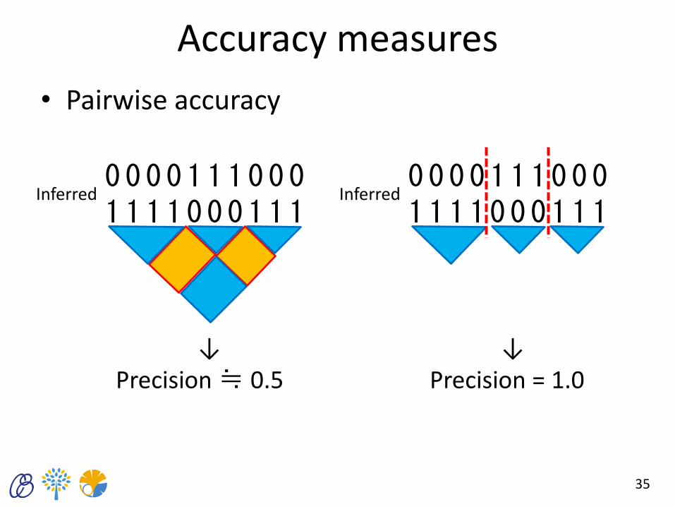
Accuracy measures
• Pairwise accuracy
35
0 0 0 0 1 1 1 0 0 0 1 1 1 1 0 0 0 1 1 1
Inferred 0 0 0 0 1 1 1 0 0 0 1 1 1 1 0 0 0 1 1 1
Inferred
↓ ↓ Precision ≒ 0.5 Precision = 1.0

Comparison of Pairwise Accuracies
• The allows indicate the threshold of MC.
36
Simulation data Real data

Comparison of Pairwise Accuracies
• The precisions without MC threshold is almost same.
37
Simulation data Real data

Comparison of Pairwise Accuracies
• The precision of MixSIH increases with high MC threshold.
38
Simulation data Real data
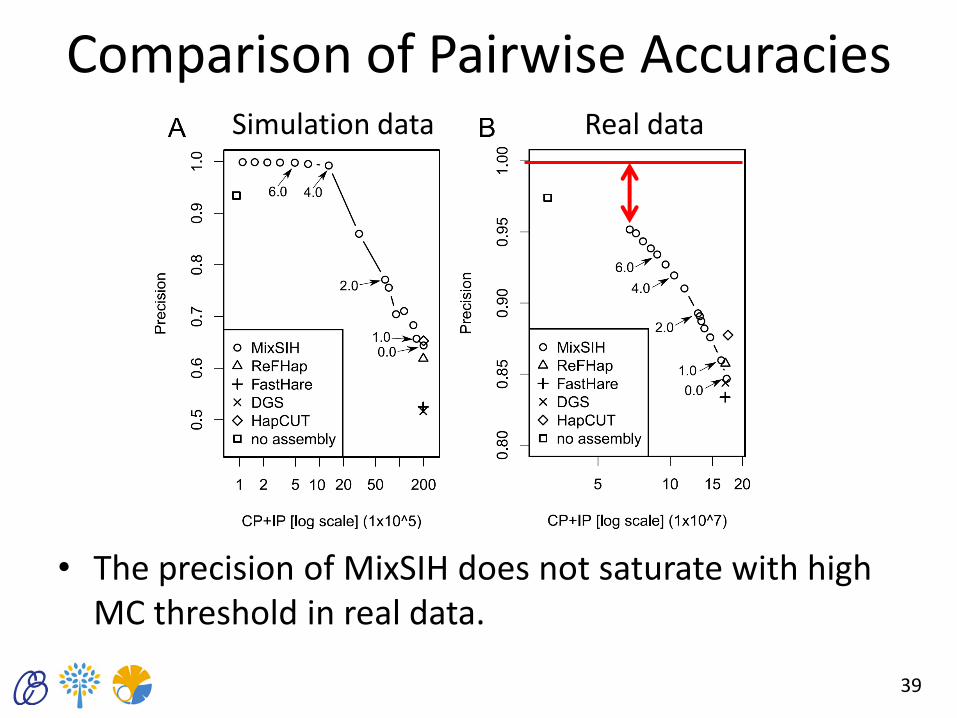
Comparison of Pairwise Accuracies
• The precision of MixSIH does not saturate with high MC threshold in real data.
39
Simulation data Real data

Problem of fosmid pool-based NGS
• Fosmid pool-based NGS has potential to produce chimeric fragment accidentally.
40
homologous
① ②
③
④
① ② ③④

• Calculate the “chimerity” of the fragment by comparing the true haplotypes data.
• Remove the fragments whose chimerity are over 10 which correspond to the case that 1.65% of the fragments were removed.
41
Remove the chimeric fragments
where n(f,h) is the number of sites at which the fragment f matches with the true haplotype h f<=i and f>j represent the left and right parts of the fragment f divided at site j, and α0=0.028 is The empirical sequence error rate.

Pairwise accuracy on the real data in which the chimeric fragments are removed
• The precision of MixSIH reaches that of unassembled prediction.
42
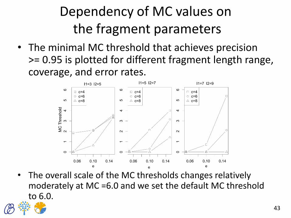
Dependency of MC values on the fragment parameters
• The minimal MC threshold that achieves precision >= 0.95 is plotted for different fragment length range, coverage, and error rates.
• The overall scale of the MC thresholds changes relatively moderately at MC =6.0 and we set the default MC threshold to 6.0.
43
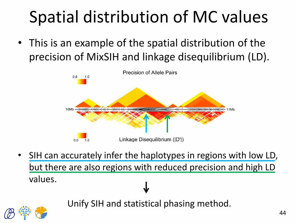
Spatial distribution of MC values
44
• This is an example of the spatial distribution of the precision of MixSIH and linkage disequilibrium (LD).
• SIH can accurately infer the haplotypes in regions with low LD, but there are also regions with reduced precision and high LD values.
Unify SIH and statistical phasing method.

Optimality of inferred parameters
• Test whether our iterative optimization method succeed to avoid sub-optimal solutions.
• The parameters converge to the global optimum upon repeating the twist operation.
45

Running time
• Our method applies the VBEM algorithm repeatedly and hence is rather slow.
• Considering the number of heterozygous sites, it is roguhly estimated that MixSIH takes about 15 days to finish haplotyping for the chromosome-wide data.
46

Conclusion
• We have developed a probabilistic model for SIH and defined the minimal connectivity (MC) score.
• Our algorithm can extract highly accurate haplotype regions by using MC values.
• We have also found evidence that there are a small number of chimeric fragments in an existing dataset of fosmid pool-based NGS, and these fragments considerably reduce the quality of the SIH.
47
Acknowledgement • Department of Computational Biology, the University of Tokyo
– Hisanori Kiryu
– Kiryu Lab. Members
• Tsukasa Fukunaga
• Yuki Kashihara
• Risa Kawaguchi
48


