
MIT OpenCourseWare http://ocw.mit.edu
6.047 / 6.878 Computational Biology: Genomes, Networks, EvolutionFall 2008
For information about citing these materials or our Terms of Use, visit: http://ocw.mit.edu/terms.
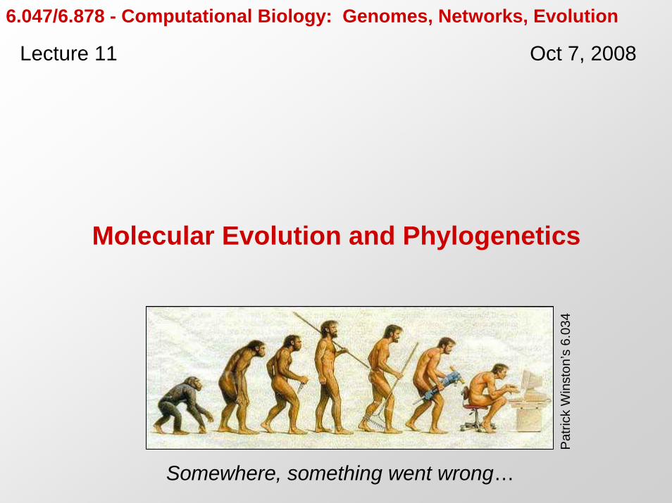
Molecular Evolution and Phylogenetics
6.047/6.878 - Computational Biology: Genomes, Networks, Evolution
Lecture 11 Oct 7, 2008
Somewhere, something went wrong…
Pat
rick
Win
ston
’s 6
.034

Challenges in Computational Biology
DNA
4 Genome Assembly
Gene FindingRegulatory motif discovery
Database lookup
Gene expression analysis9
RNA transcript
Sequence alignment
Evolutionary Theory7TCATGCTATTCGTGATAATGAGGATATTTATCATATTTATGATTT
Cluster discovery10 Gibbs samplingProtein network analysis12
Emerging network properties14
13 Regulatory network inference
Comparative Genomics
RNA folding
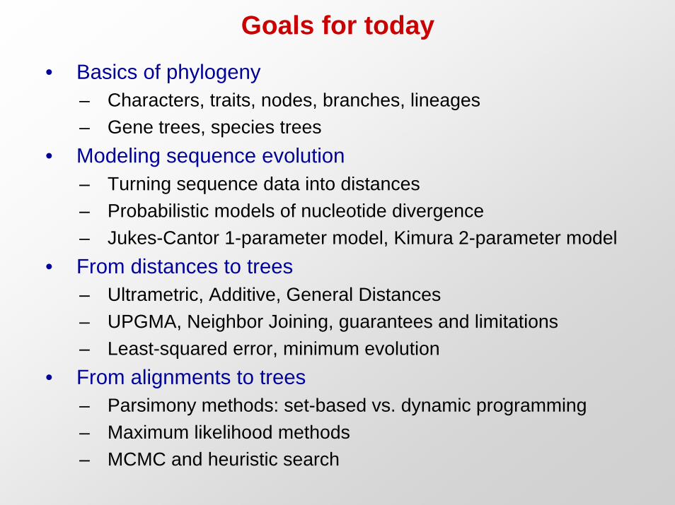
Goals for today• Basics of phylogeny
– Characters, traits, nodes, branches, lineages– Gene trees, species trees
• Modeling sequence evolution– Turning sequence data into distances– Probabilistic models of nucleotide divergence– Jukes-Cantor 1-parameter model, Kimura 2-parameter model
• From distances to trees– Ultrametric, Additive, General Distances– UPGMA, Neighbor Joining, guarantees and limitations– Least-squared error, minimum evolution
• From alignments to trees– Parsimony methods: set-based vs. dynamic programming– Maximum likelihood methods– MCMC and heuristic search

Open questions (?)
• Panda– Bear or raccoon?
• Out of Africa– mitochondrial evolution story?
• Human evolution– Did we ever meet Neanderthal?
• Primate evolution– Are we chimp-like or gorilla-like?
• Vertebrate evolution– How did complex body plans arise?
• Recent evolution– What genes are under selection?
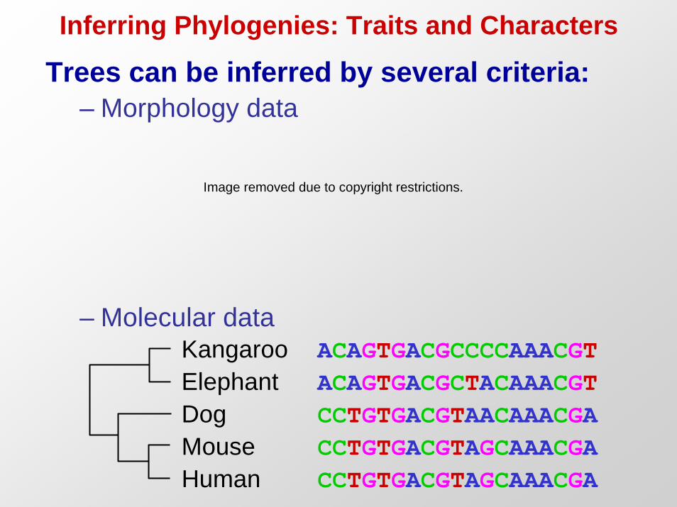
Inferring Phylogenies: Traits and Characters
Trees can be inferred by several criteria:– Morphology data
– Molecular dataKangaroo ACAGTGACGCCCCAAACGTElephant ACAGTGACGCTACAAACGTDog CCTGTGACGTAACAAACGAMouse CCTGTGACGTAGCAAACGAHuman CCTGTGACGTAGCAAACGA
Image removed due to copyright restrictions.
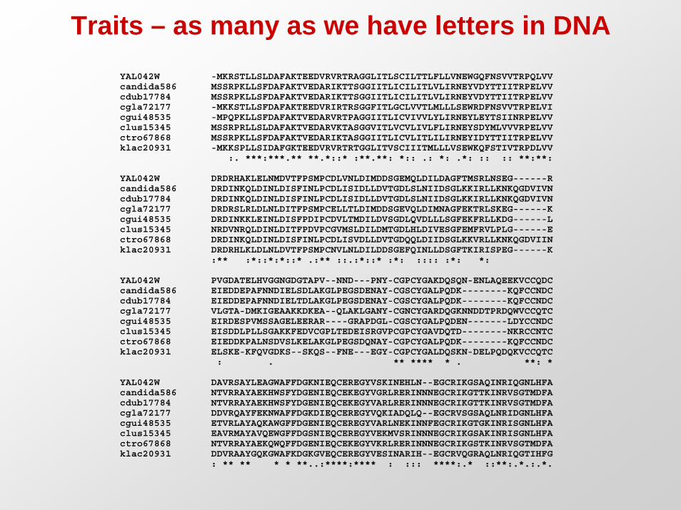
Traits – as many as we have letters in DNAYAL042W -MKRSTLLSLDAFAKTEEDVRVRTRAGGLITLSCILTTLFLLVNEWGQFNSVVTRPQLVVcandida586 MSSRPKLLSFDAFAKTVEDARIKTTSGGIITLICILITLVLIRNEYVDYTTIITRPELVVcdub17784 MSSRPKLLSFDAFAKTVEDARIKTTSGGIITLICILITLVLIRNEYVDYTTIITRPELVVcgla72177 -MKKSTLLSFDAFAKTEEDVRIRTRSGGFITLGCLVVTLMLLLSEWRDFNSVVTRPELVIcgui48535 -MPQPKLLSFDAFAKTVEDARVRTPAGGIITLICVIVVLYLIRNEYLEYTSIINRPELVVclus15345 MSSRPRLLSLDAFAKTVEDARVKTASGGVITLVCVLIVLFLIRNEYSDYMLVVVRPELVVctro67868 MSSRPKLLSFDAFAKTVEDARIKTASGGIITLICVLITLILIRNEYIDYTTIITRPELVVklac20931 -MKKSPLLSIDAFGKTEEDVRVRTRTGGLITVSCIIITMLLLVSEWKQFSTIVTRPDLVV
:. ***:***.** **.*::* :**.**: *:: .: *: .*: :: :: **:**:
YAL042W DRDRHAKLELNMDVTFPSMPCDLVNLDIMDDSGEMQLDILDAGFTMSRLNSEG------Rcandida586 DRDINKQLDINLDISFINLPCDLISIDLLDVTGDLSLNIIDSGLKKIRLLKNKQGDVIVNcdub17784 DRDINKQLDINLDISFINLPCDLISIDLLDVTGDLSLNIIDSGLKKIRLLKNKQGDVIVNcgla72177 DRDRSLRLDLNLDITFPSMPCELLTLDIMDDSGEVQLDIMNAGFEKTRLSKEG------Kcgui48535 DRDINKKLEINLDISFPDIPCDVLTMDILDVSGDLQVDLLLSGFEKFRLLKDG------Lclus15345 NRDVNRQLDINLDITFPDVPCGVMSLDILDMTGDLHLDIVESGFEMFRVLPLG------Ectro67868 DRDINKQLDINLDISFINLPCDLISVDLLDVTGDQQLDIIDSGLKKVRLLKNKQGDVIINklac20931 DRDRHLKLDLNLDVTFPSMPCNVLNLDILDDSGEFQINLLDSGFTKIRISPEG------K
:** :*::*:*::* .:** ::.:*::* :*: :::: :*: *:
YAL042W PVGDATELHVGGNGDGTAPV--NND---PNY-CGPCYGAKDQSQN-ENLAQEEKVCCQDCcandida586 EIEDDEPAFNNDIELSDLAKGLPEGSDENAY-CGSCYGALPQDK--------KQFCCNDCcdub17784 EIEDDEPAFNNDIELTDLAKGLPEGSDENAY-CGSCYGALPQDK--------KQFCCNDCcgla72177 VLGTA-DMKIGEAAKKDKEA--QLAKLGANY-CGNCYGARDQGKNNDDTPRDQWVCCQTCcgui48535 EIRDESPVMSSAGELEERAR----GRAPDGL-CGSCYGALPQDEN-------LDYCCNDCclus15345 EISDDLPLLSGAKKFEDVCGPLTEDEISRGVPCGPCYGAVDQTD--------NKRCCNTCctro67868 EIEDDKPALNSDVSLKELAKGLPEGSDQNAY-CGPCYGALPQDK--------KQFCCNDCklac20931 ELSKE-KFQVGDKS--SKQS--FNE---EGY-CGPCYGALDQSKN-DELPQDQKVCCQTC
: . ** **** * . **: *
YAL042W DAVRSAYLEAGWAFFDGKNIEQCEREGYVSKINEHLN--EGCRIKGSAQINRIQGNLHFAcandida586 NTVRRAYAEKHWSFYDGENIEQCEKEGYVGRLRERINNNEGCRIKGTTKINRVSGTMDFAcdub17784 NTVRRAYAEKHWSFYDGENIEQCEKEGYVARLRERINNNEGCRIKGTTKINRVSGTMDFAcgla72177 DDVRQAYFEKNWAFFDGKDIEQCEREGYVQKIADQLQ--EGCRVSGSAQLNRIDGNLHFAcgui48535 ETVRLAYAQKAWGFFDGENIEQCEREGYVARLNEKINNFEGCRIKGTGKINRISGNLHFAclus15345 EAVRMAYAVQEWGFFDGSNIEQCEREGYVEKMVSRINNNEGCRIKGSAKINRISGNLHFActro67868 NTVRRAYAEKQWQFFDGENIEQCEKEGYVKRLRERINNNEGCRIKGSTKINRVSGTMDFAklac20931 DDVRAAYGQKGWAFKDGKGVEQCEREGYVESINARIH--EGCRVQGRAQLNRIQGTIHFG
: ** ** * * **..:****:**** : ::: ****:.* ::**:.*.:.*.
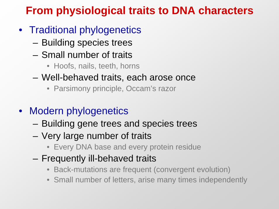
From physiological traits to DNA characters
• Traditional phylogenetics– Building species trees– Small number of traits
• Hoofs, nails, teeth, horns– Well-behaved traits, each arose once
• Parsimony principle, Occam’s razor
• Modern phylogenetics– Building gene trees and species trees– Very large number of traits
• Every DNA base and every protein residue– Frequently ill-behaved traits
• Back-mutations are frequent (convergent evolution)• Small number of letters, arise many times independently
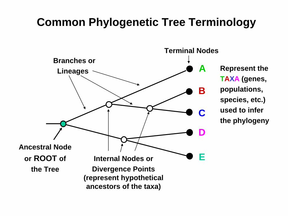
Ancestral Nodeor ROOT of
the TreeInternal Nodes orDivergence Points
(represent hypothetical ancestors of the taxa)
Branches orLineages
Terminal Nodes
A
B
C
D
E
Represent theTAXA (genes,populations,species, etc.)used to inferthe phylogeny
Common Phylogenetic Tree Terminology
Taxon A
Taxon B
Taxon C
Taxon D
11
1
6
3
5
genetic change
Taxon A
Taxon B
Taxon C
Taxon D
time
Taxon A
Taxon B
Taxon C
Taxon D
no meaning
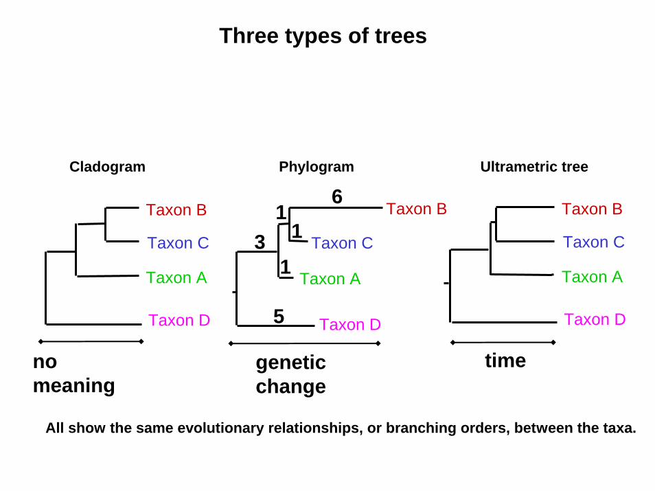
Three types of trees
Cladogram Phylogram Ultrametric tree
All show the same evolutionary relationships, or branching orders, between the taxa.
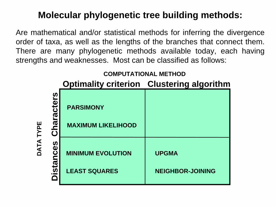
Molecular phylogenetic tree building methods:
Are mathematical and/or statistical methods for inferring the divergence order of taxa, as well as the lengths of the branches that connect them. There are many phylogenetic methods available today, each havingstrengths and weaknesses. Most can be classified as follows:
COMPUTATIONAL METHOD
Clustering algorithmOptimality criterion
Cha
ract
ers
Dis
tanc
es
PARSIMONY
MAXIMUM LIKELIHOOD
UPGMA
NEIGHBOR-JOINING
MINIMUM EVOLUTION
LEAST SQUARES
DA
TA T
YPE
2. Modeling evolution
Inferring evolutionary distance
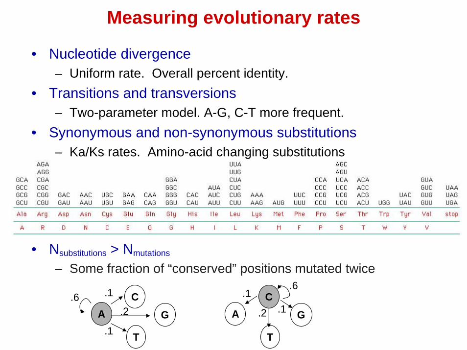
Measuring evolutionary rates
• Nucleotide divergence– Uniform rate. Overall percent identity.
• Transitions and transversions– Two-parameter model. A-G, C-T more frequent.
• Synonymous and non-synonymous substitutions– Ka/Ks rates. Amino-acid changing substitutions
• Nsubstitutions > Nmutations
– Some fraction of “conserved” positions mutated twice
AC
G
T
AC
G
T
.1
.1
.2.6
.6.1
.2 .1
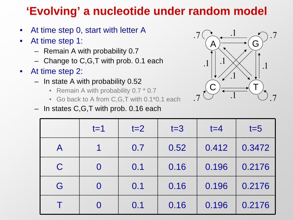
‘Evolving’ a nucleotide under random model
A G
C T
.1
.1.1
.1
.1
.1
.7.7
.7.7
• At time step 0, start with letter A• At time step 1:
– Remain A with probability 0.7– Change to C,G,T with prob. 0.1 each
• At time step 2: – In state A with probability 0.52
• Remain A with probability 0.7 * 0.7• Go back to A from C,G,T with 0.1*0.1 each
– In states C,G,T with prob. 0.16 each
t=1 t=2 t=3 t=4 t=5
A 1 0.7 0.52 0.412 0.3472
C 0 0.1 0.16 0.196 0.2176
G 0 0.1 0.16 0.196 0.2176
T 0 0.1 0.16 0.196 0.2176

Modeling Nucleotide EvolutionDuring infinitesimal time Δt, there is not enough time for two
substitutions to happen on the same nucleotide
So we can estimate P(x | y, Δt), for x, y ∈ {A, C, G, T}
Then let
P(A|A, Δt) …… P(A|T, Δt)S(Δt) = … …
P(T|A, Δt) …… P(T|T, Δt)
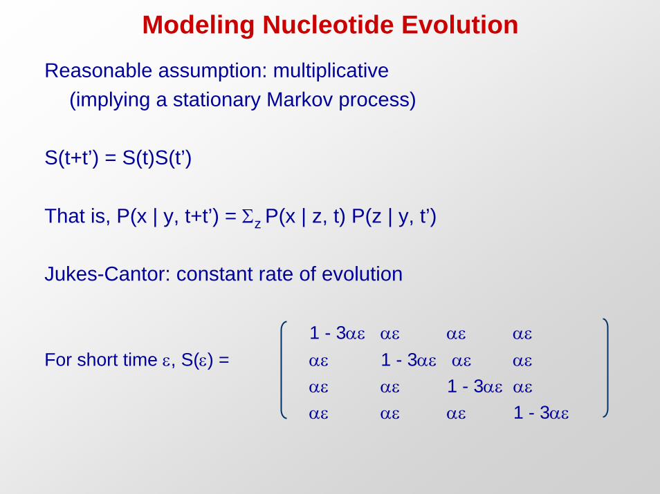
Modeling Nucleotide EvolutionReasonable assumption: multiplicative
(implying a stationary Markov process)
S(t+t’) = S(t)S(t’)
That is, P(x | y, t+t’) = Σz P(x | z, t) P(z | y, t’)
Jukes-Cantor: constant rate of evolution
1 - 3αε αε αε αεFor short time ε, S(ε) = αε 1 - 3αε αε αε
αε αε 1 - 3αε αεαε αε αε 1 - 3αε
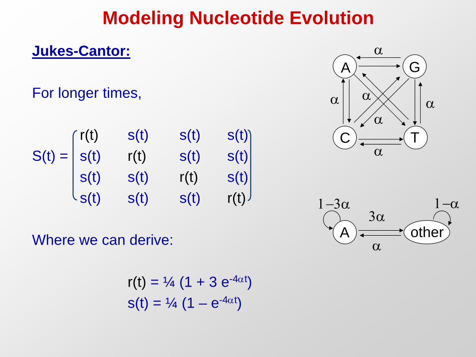
Modeling Nucleotide EvolutionJukes-Cantor:
For longer times,
r(t) s(t) s(t) s(t)S(t) = s(t) r(t) s(t) s(t)
s(t) s(t) r(t) s(t)s(t) s(t) s(t) r(t)
Where we can derive:
r(t) = ¼ (1 + 3 e-4αt)s(t) = ¼ (1 – e-4αt)
A G
C T
A other3α
1−3α
α
1−α
α
αα
α
α
α

Modeling Nucleotide Evolution
Kimura:
Transitions: A/G, C/TTransversions: A/T, A/C, G/T, C/G
Transitions (rate α) are much more likely than transversions (rate β)
r(t) s(t) u(t) u(t)S(t) = s(t) r(t) u(t) u(t)
u(t) u(t) r(t) s(t)u(t) u(t) s(t) r(t)
Where s(t) = ¼ (1 – e-4βt)u(t) = ¼ (1 + e-4βt – e-2(α+β)t)r(t) = 1 – 2s(t) – u(t)
A G C T
AG
C
T

Distance between two sequences
Given (well-aligned portion of) sequences xi, xj,
Define dij = distance between the two sequences
One possible definition:dij = fraction f of sites u where xi[u] ≠ xj[u]
Better model (Jukes-Cantor):dij = - ¾ log(1 – 4f / 3)
r(t) = ¼ (1 + 3 e-4αt)s(t) = ¼ (1 – e-4αt)
Observed F = [ 0.1, 0.2, 0.3, 0.4, 0.5, 0.6, 0.7])Actual D = [0.11, 0.23, 0.38, 0.57, 0.82, 1.21, 2.03]
3. From distances to trees
Ultrametric, additive, and generaldistance matrices
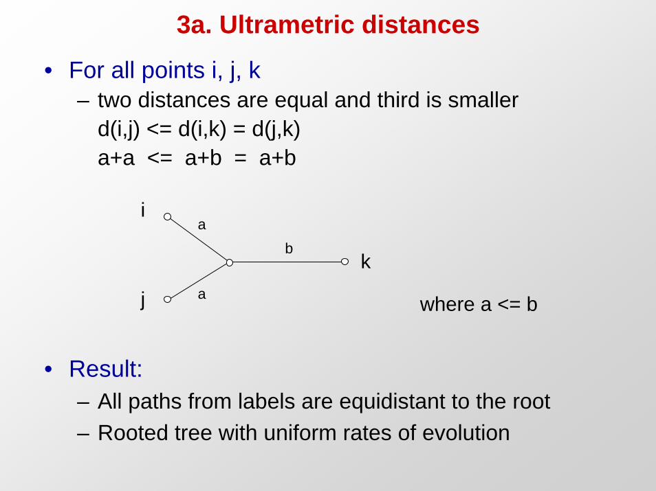
3a. Ultrametric distances
• For all points i, j, k– two distances are equal and third is smaller
d(i,j) <= d(i,k) = d(j,k)a+a <= a+b = a+b
a
a
b
i
j
k
where a <= b
• Result: – All paths from labels are equidistant to the root– Rooted tree with uniform rates of evolution
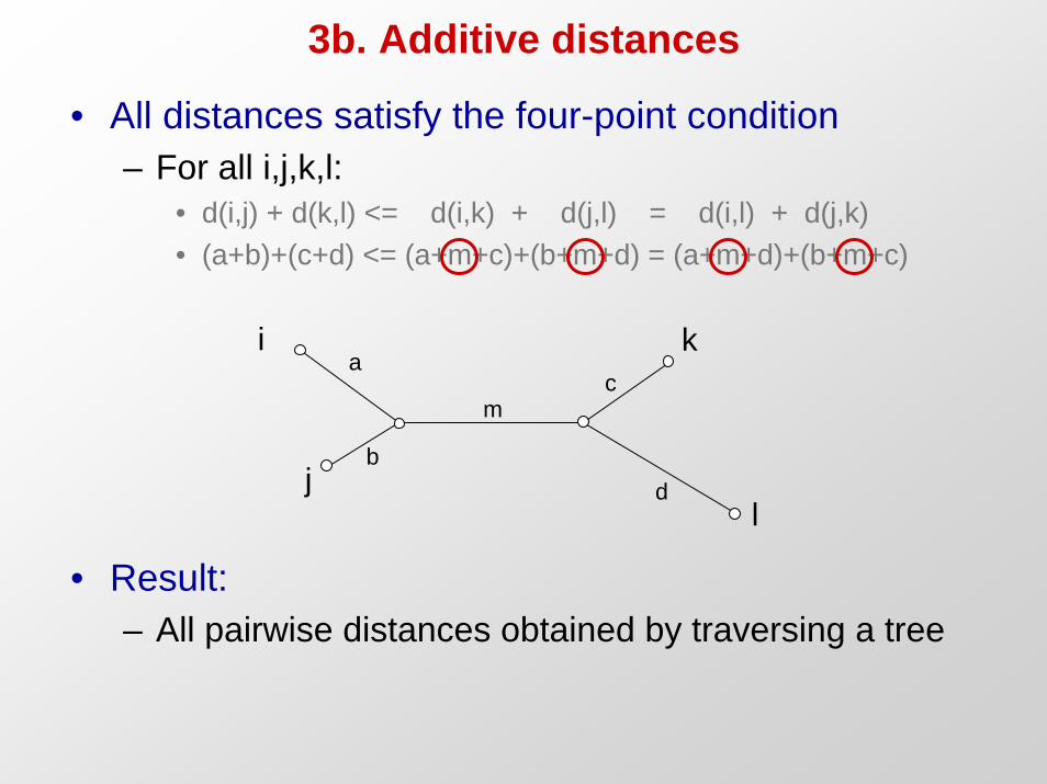
3b. Additive distances
• All distances satisfy the four-point condition– For all i,j,k,l:
• d(i,j) + d(k,l) <= d(i,k) + d(j,l) = d(i,l) + d(j,k)• (a+b)+(c+d) <= (a+m+c)+(b+m+d) = (a+m+d)+(b+m+c)
• Result: – All pairwise distances obtained by traversing a tree
a
b
m
i
j
k
l
c
d
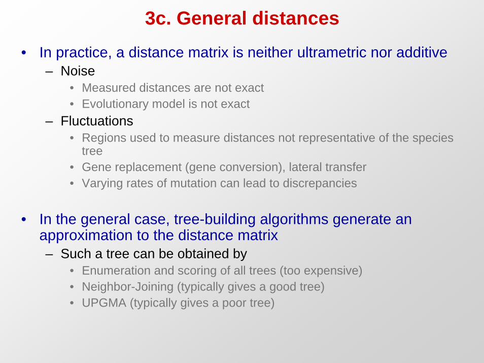
3c. General distances• In practice, a distance matrix is neither ultrametric nor additive
– Noise• Measured distances are not exact• Evolutionary model is not exact
– Fluctuations• Regions used to measure distances not representative of the species
tree• Gene replacement (gene conversion), lateral transfer• Varying rates of mutation can lead to discrepancies
• In the general case, tree-building algorithms generate an approximation to the distance matrix– Such a tree can be obtained by
• Enumeration and scoring of all trees (too expensive)• Neighbor-Joining (typically gives a good tree)• UPGMA (typically gives a poor tree)
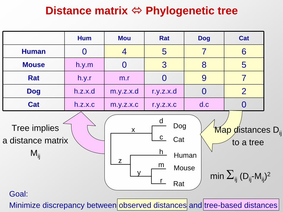
Distance matrix Phylogenetic tree
Hum Mou Rat Dog Cat
Human 0 4 5 7 6Mouse h.y.m 0 3 8 5
Rat h.y.r m.r 0 9 7Dog h.z.x.d m.y.z.x.d r.y.z.x.d 0 2Cat h.z.x.c m.y.z.x.c r.y.z.x.c d.c 0
Human
Dog
Cat
Mouse
Rat
d
cx
hz m
yr
Goal: Minimize discrepancy between observed distances and tree-based distances
Map distances Dij
to a treeTree implies
a distance matrixMij
min Σij (Dij-Mij)2
4. Tree-building algorithms
Mapping a distance matrix to a tree
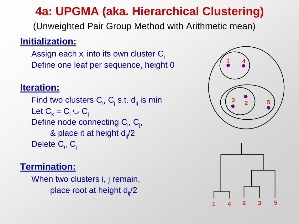
4a: UPGMA (aka. Hierarchical Clustering)
Initialization:Assign each xi into its own cluster Ci
Define one leaf per sequence, height 0
Iteration:Find two clusters Ci, Cj s.t. dij is minLet Ck = Ci ∪ CjDefine node connecting Ci, Cj,
& place it at height dij/2Delete Ci, Cj
Termination:When two clusters i, j remain,
place root at height dij/2
1 4
3 2 5
1 4 2 3 5
(Unweighted Pair Group Method with Arithmetic mean)
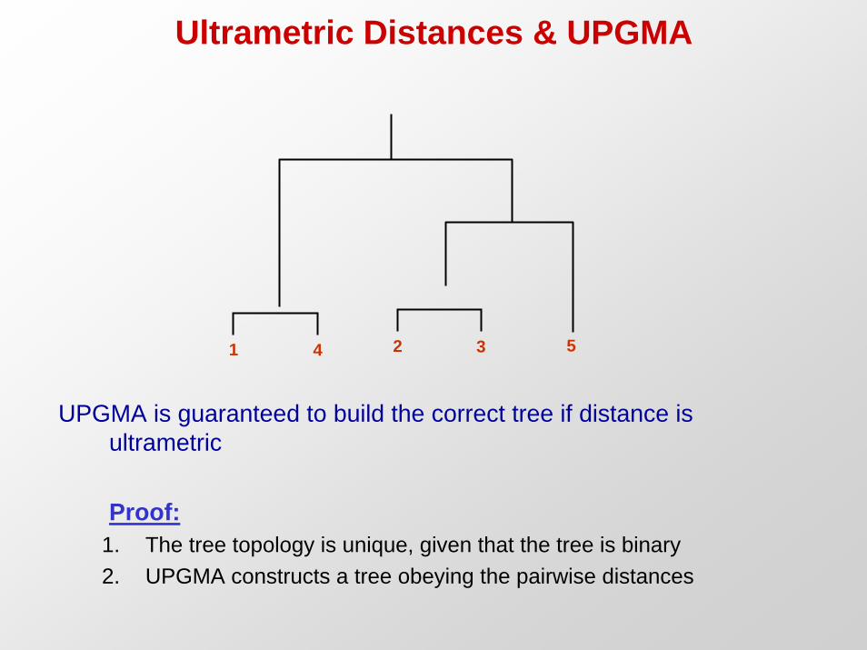
Ultrametric Distances & UPGMA
UPGMA is guaranteed to build the correct tree if distance is ultrametric
Proof:1. The tree topology is unique, given that the tree is binary2. UPGMA constructs a tree obeying the pairwise distances
1 4 2 3 5
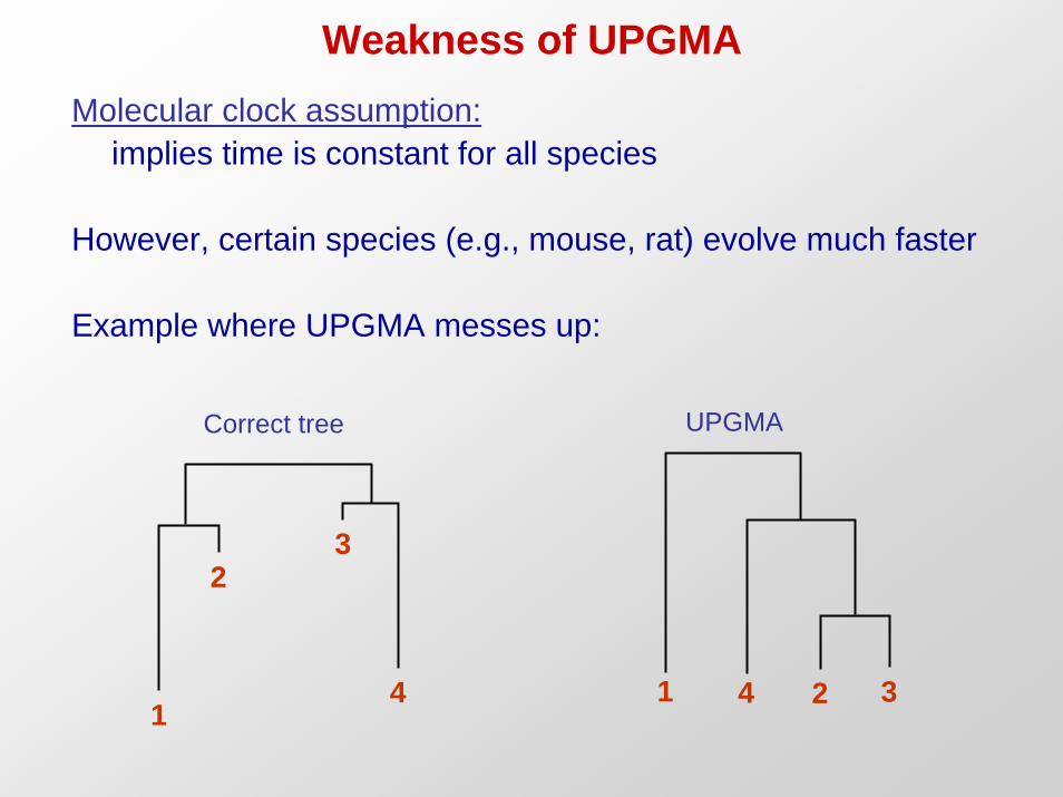
Weakness of UPGMAMolecular clock assumption:
implies time is constant for all species
However, certain species (e.g., mouse, rat) evolve much faster
Example where UPGMA messes up:
23
41
1 4 32
Correct tree UPGMA
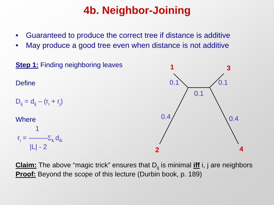
4b. Neighbor-Joining
• Guaranteed to produce the correct tree if distance is additive• May produce a good tree even when distance is not additive
Step 1: Finding neighboring leaves
Define
Dij = dij – (ri + rj)
Where1
ri = –––––Σk dik|L| - 2
Claim: The above “magic trick” ensures that Dij is minimal iff i, j are neighborsProof: Beyond the scope of this lecture (Durbin book, p. 189)
1
2 4
0.1 0.1
0.4 0.4
3
0.1
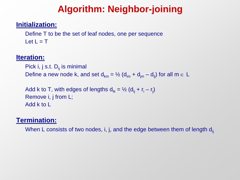
Algorithm: Neighbor-joiningInitialization:
Define T to be the set of leaf nodes, one per sequenceLet L = T
Iteration:Pick i, j s.t. Dij is minimalDefine a new node k, and set dkm = ½ (dim + djm – dij) for all m ∈ L
Add k to T, with edges of lengths dik = ½ (dij + ri – rj)Remove i, j from L; Add k to L
Termination:When L consists of two nodes, i, j, and the edge between them of length dij

5. Alignment-based algorithms
Parsimony (set-based)Parsimony (Dynamic Programming)
Maximum Likelihood
5a. Parsimony• One of the most popular methods
Idea:Find the tree that explains the observed sequences with a minimal number of substitutions
Two computational sub-problems:
1. Find the parsimony cost of a given tree (easy)
2. Search through all tree topologies (hard)
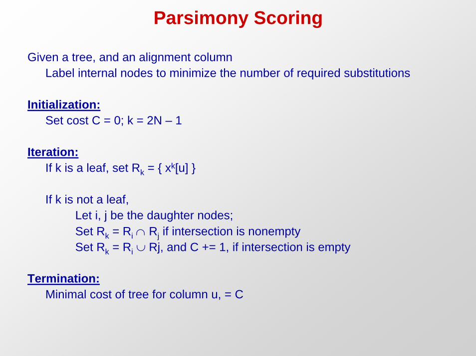
Parsimony Scoring
Given a tree, and an alignment columnLabel internal nodes to minimize the number of required substitutions
Initialization:Set cost C = 0; k = 2N – 1
Iteration:If k is a leaf, set Rk = { xk[u] }
If k is not a leaf,Let i, j be the daughter nodes;Set Rk = Ri ∩ Rj if intersection is nonemptySet Rk = Ri ∪ Rj, and C += 1, if intersection is empty
Termination:Minimal cost of tree for column u, = C

Example
A B B
{A, B}C+=1
{A, B}C+=1
{A}
{A} {B} {A} {B}A
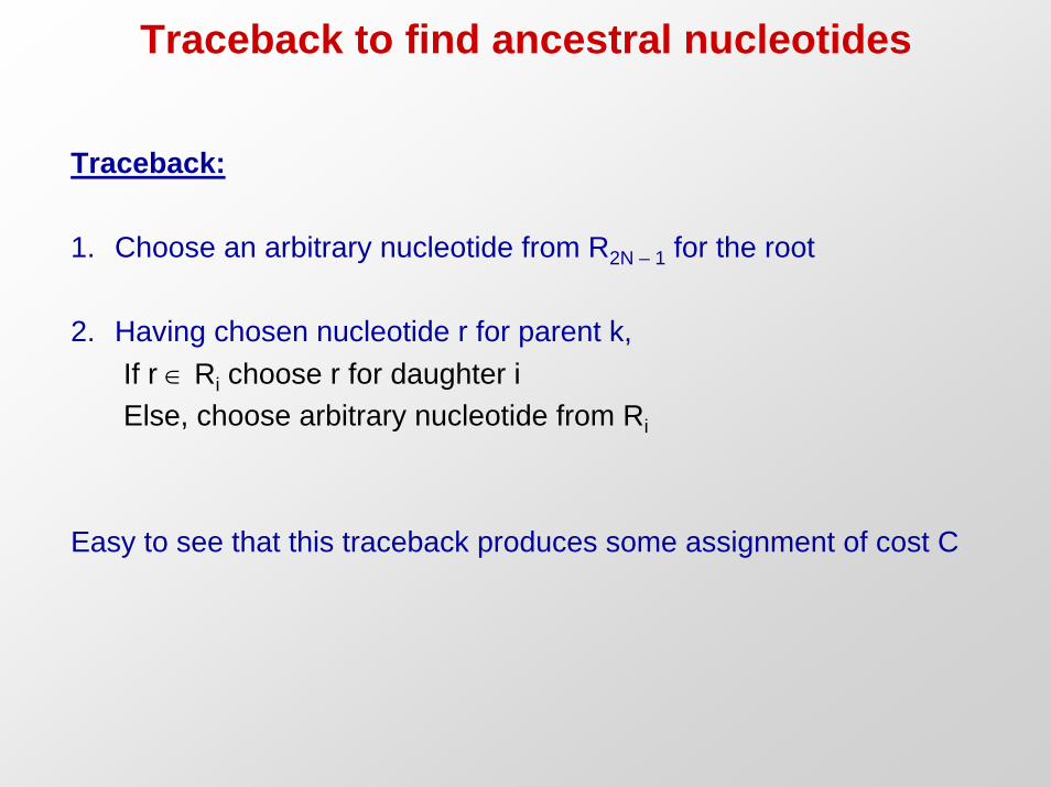
Traceback:
1. Choose an arbitrary nucleotide from R2N – 1 for the root
2. Having chosen nucleotide r for parent k, If r ∈ Ri choose r for daughter iElse, choose arbitrary nucleotide from Ri
Easy to see that this traceback produces some assignment of cost C
Traceback to find ancestral nucleotides
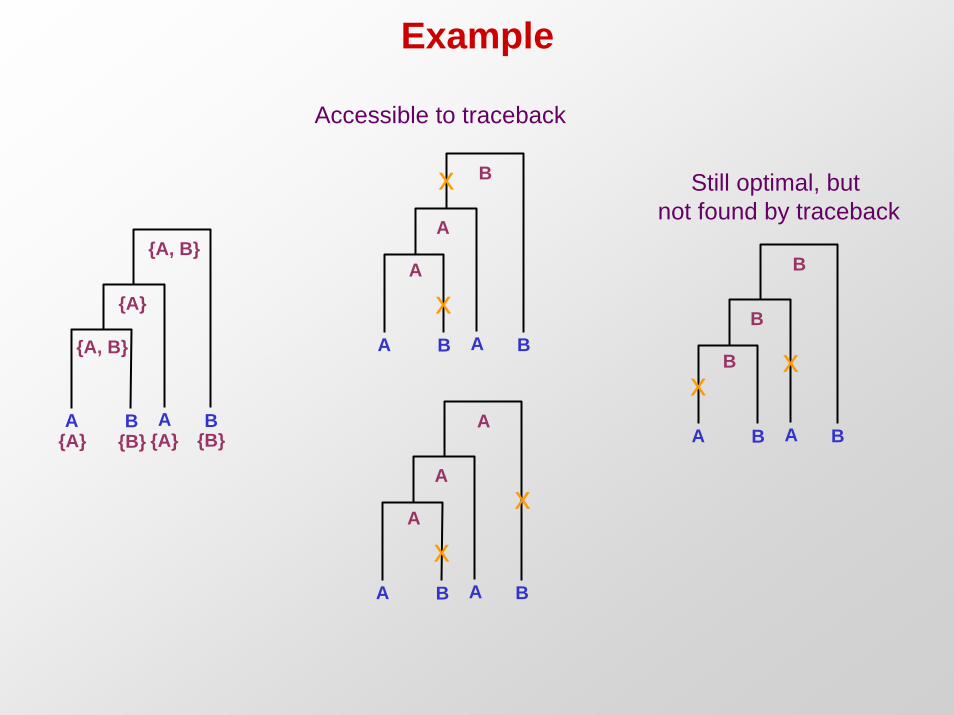
Example
A B A B
{A, B}
{A, B}
{A}
{A} {B} {A} {B}
A B A B
A
A
Ax
x
A B A B
A
B
A
x
x
A B A B
B
B
B
xx
Accessible to traceback
Still optimal, but not found by traceback
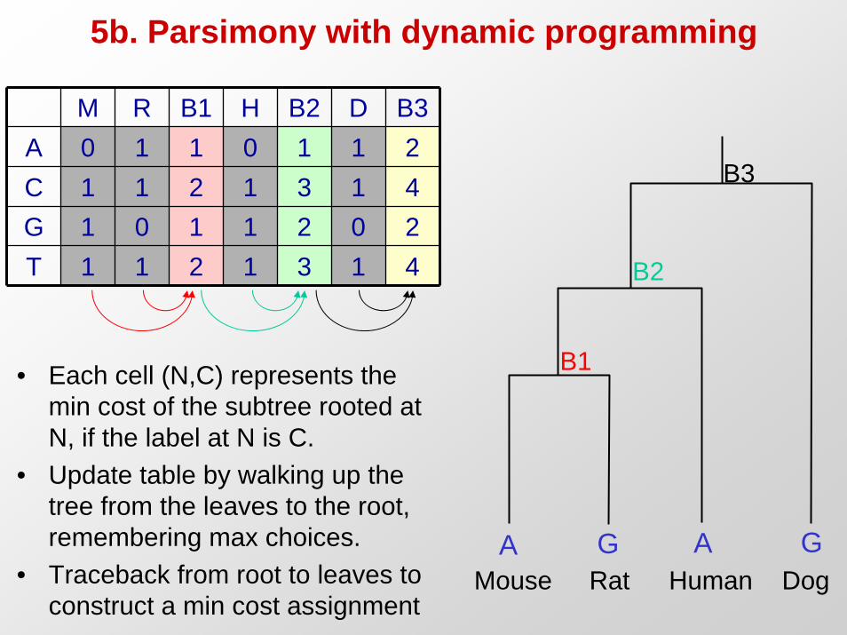
5b. Parsimony with dynamic programming
M R B1 H B2 D B3A 0 1 1 0 1 1 2C 1 1 2 1 3 1 4G 1 0 1 1 2 0 2T 1 1 2 1 3 1 4
• Each cell (N,C) represents the min cost of the subtree rooted at N, if the label at N is C.
• Update table by walking up the tree from the leaves to the root, remembering max choices.
• Traceback from root to leaves to construct a min cost assignment
A G A GMouse Rat Human Dog
B1
B2
B3

5c. Maximum Likelihood MethodsInput: Proposed topology TOutput: Prob. that proposed tree gave rise to observed dataSearch: Heuristic MCMC search for max likelihood tree.
B^,T^ = argmaxB,T P(D,B,T)= argmaxB,T P(D|B,T) P(B,T)
Likelihood P(Data|BranchLengths,Topology)Prior P(B,T): typically uniform/can use to guide search
Iterate: Iterate over proposed topologies. • Given current topology T, branch lengths B:
– Propose many alternative (T’,B’), by modifying existing T T’, and inferring branch lengths B’ that maximize P(D|B’,T’)
– Evaluate P(D|B,T) and P(D|B’,T’)– Select one T’ at random based on increase in likelihood
• Heuristics for proposing new topology T’– Nearest-neighbor interchange, subtree cut-and-paste, rotations
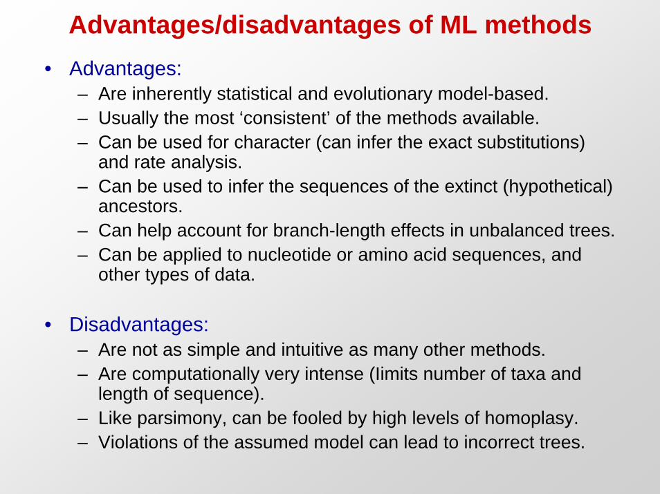
Advantages/disadvantages of ML methods• Advantages:
– Are inherently statistical and evolutionary model-based.– Usually the most ‘consistent’ of the methods available.– Can be used for character (can infer the exact substitutions)
and rate analysis.– Can be used to infer the sequences of the extinct (hypothetical)
ancestors.– Can help account for branch-length effects in unbalanced trees.– Can be applied to nucleotide or amino acid sequences, and
other types of data.
• Disadvantages:– Are not as simple and intuitive as many other methods.– Are computationally very intense (Iimits number of taxa and
length of sequence).– Like parsimony, can be fooled by high levels of homoplasy.– Violations of the assumed model can lead to incorrect trees.
Bootstrapping to get the best trees
Main outline of algorithm
1. Select random columns from a multiple alignment – one column can then appear several times
2. Build a phylogenetic tree based on the random sample from (1)
3. Repeat (1), (2) many (say, 1000) times
4. Output the tree that is constructed most frequently

Summary• Basics of phylogeny
– Characters, traits, nodes, branches, lineages– Gene trees, species trees
• Modeling sequence evolution– Turning sequence data into distances– Probabilistic models of nucleotide divergence– Jukes-Cantor 1-parameter model, Kimura 2-parameter model
• From distances to trees– Ultrametric, Additive, General Distances– UPGMA, Neighbor Joining, guarantees and limitations– Least-squared error, minimum evolution
• From alignments to trees– Parsimony methods: set-based vs. dynamic programming– Maximum likelihood methods– MCMC and heuristic search

Extra Time?

Recitation tomorrow: Gene vs. Species evolution• Genes can start diverging before species separate
– Genetic polymorphism within population could exist– After divergence, forms evolve differently in each species– Gene divergence could predate species diverge– Gene tree topology could be misleading
A
B
X Y Z
AB
X Y Z
• Solution: Use multiple genes to infer a species tree
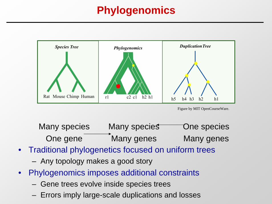
Phylogenomics
• Traditional phylogenetics focused on uniform trees– Any topology makes a good story
• Phylogenomics imposes additional constraints– Gene trees evolve inside species trees– Errors imply large-scale duplications and losses
Many speciesOne gene
One speciesMany genes
Many speciesMany genes
h1r1 c1c2 h2 h1 h2h3h4h5HumanChimpMouseRat
Species Tree Phylogenomics Duplication Tree
Figure by MIT OpenCourseWare.

Extending traditional max likelihood methods
• Traditional max likelihood (phylogenetics)
B^,T^ = argmaxB,T P(D,B,T)argmaxB,T P(D|B,T) P(B,T)
• Extended likelihood function (phylogenomics)
B^,T^ = argmaxB,T P(D,B,T,R|E)argmaxB,T P(D|B,T) P(B|T,R,E)P(R|T,E)P(T|E)
Likelihood of data givenproposed branch lengths
Likelihood of proposed branch lengths (given species evolution)
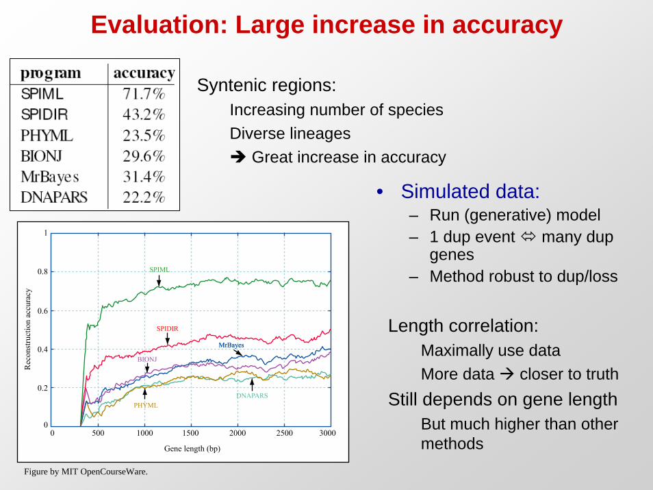
Evaluation: Large increase in accuracy
• Simulated data: – Run (generative) model– 1 dup event many dup
genes– Method robust to dup/loss
Syntenic regions: Increasing number of speciesDiverse lineages
Great increase in accuracy
Length correlation: Maximally use dataMore data closer to truth
Still depends on gene lengthBut much higher than other methods
Rec
onst
ruct
ion
accu
racy
0
0.2
0.4
0.6
0.8
1
Gene length (bp)
0 500 1000 1500 2000 2500 3000
SPIML
DNAPARSPHYML
SPIDIR
BIONJ
MrBayesMrBayes
Figure by MIT OpenCourseWare.


