Mathematical modelling of some aspects of
intracellular second messenger signalling
Greg LemonS
IDERE ·ME
NS ·EADE
M·MUTAT
O
A thesis submitted in fulfilmentof the requirements for the degree of
Doctor of Philosophy
School of Mathematics and Statistics
University of Sydney
August, 2003
Declaration
The work presented in this thesis is a result of my own investigation unless otherwise
stated. No material contained in this thesis has been accepted for the award of a degree
or diploma at any other university.
Greg Lemon.
October 3, 2003
i
Author’s Note
Most of the material contained in this thesis also appears in the form of refereed journal
articles.
Chapters 2, 3 and 4 have been published as the papers Lemon et al. (2003a), Lemon
et al. (2003b) and Lemon et al. (2003d) respectively, with only minor textual changes.
Part of Chapter 2 also appears in the article Lemon et al. (2003c), which is a conference
paper presented at the Annual Computational Neuroscience meeting, 2002. The results
of Chapters 2 and 3 were the subject of the conference presentation Lemon et al. (2002).
The material that has not appeared elsewhere consists of (a) the introduction, Chapter
1 and (b) the subsection of Appendix C dealing with the case of fast membrane kinetics
for the interaction of GFP-PHD with the cell membrane.
ii
Abstract
This thesis contains a theoretical investigation of several different aspects of second
messenger signalling inside single cells, using mathematical modelling techniques. The
thesis is divided into three parts.
In the first part, a detailed mathematical model is presented governing the dynamics of
subcellular chemical species, starting from the application of external ligand through
to the production of inositol 1,4,5-trisphosphate (IP3) and ultimately to the release of
Ca2+ from internal stores. The model is then used to quantify experimental data of
the purinergic stimulation of 1321N1 human astrocytoma cells (Garrad et al., J. Biol.
Chem. 273 (1998), 29437-29444).
In the second part, a mathematical model is presented for the dynamics of the Green
Fluorescent Protein-Pleckstrin Homology Domain (GFP-PHD) fusion construct. Bound-
ary layer techniques are used to derive a simplified set of equations that describe
changes in cytosolic and membrane GFP-PHD fluorescence. These equations are used
to deduce the spatial and temporal changes of IP3 concentrations inside cells. The
model is also used in conjunction with the complete signal transduction model from
the first part to quantify GFP-PHD fluorescence data of the purinergic stimulation of
Madin-Darby canine kidney epithelial cells (Hirose et al., Science 284 (1999), 1527-
1530).
In the third part of the thesis, the propagation of saltatory calcium waves through
confined intracellular spaces is considered. The existence, stability and speed of these
waves are shown to depend critically on the values of the model parameters. The
results are applied to the case of calcium waves propagating in the subsarcolemmal
regions of atrial myocytes (Kockskamper et al., Biophys. J. 81 (2001), 2590-2605).
iii

Acknowledgements
Firstly I wish to thank my supervisor, Associate Professor Bill Gibson, and my associate
supervisor, Professor Max Bennett, for their support and guidance. I am indebted for
their helping to keep my work accessible to biologists.
I also wish to acknowledge the help of all staff and students of the School of Mathematics
and Statistics who in any way assisted me in my work. In particular I would like to give
thanks to my fellow PhD students Greg Woodbury and Joshua van Kleef with whom
I had many stimulating discussions. Thanks also to Charlie Macaskill and Rosemary
Thompson for their friendly encouragement. I must also give special thanks to the
administrative and computer systems staff within the school, whose kind assistance
was so important.
I gratefully acknowledge the financial support of an Australian Postgraduate Award,
Sydney University Sesqui grants U4120, U4218, U4066 and small ARC grant A2496.
Finally, I would like to thank my mother and father, whose devotion to me and their
commitment to my education made this thesis possible.
iv

Contents
1 Introduction 1
1.1 Intracellular signal transduction . . . . . . . . . . . . . . . . . . . . . . 1
1.2 Fluorescent indicators in cell biology . . . . . . . . . . . . . . . . . . . 6
1.3 Intracellular Ca2+ waves . . . . . . . . . . . . . . . . . . . . . . . . . . 11
2 Modelling calcium and inositol 1,4,5-trisphosphate dynamics follow-
ing receptor activation 18
2.1 Introduction . . . . . . . . . . . . . . . . . . . . . . . . . . . . . . . . . 18
2.2 Methods . . . . . . . . . . . . . . . . . . . . . . . . . . . . . . . . . . . 20
2.2.1 Regulation of metabotropic receptor activity . . . . . . . . . . . 20
2.2.2 G-protein cascade . . . . . . . . . . . . . . . . . . . . . . . . . . 24
2.2.3 Cytosolic Ca2+ dynamics . . . . . . . . . . . . . . . . . . . . . . 27
2.2.4 Initial conditions and methods of solution . . . . . . . . . . . . 28
2.3 Results . . . . . . . . . . . . . . . . . . . . . . . . . . . . . . . . . . . . 30
2.3.1 Model predictions for desensitization and sequestration . . . . . 30
2.3.2 Parameter value selection . . . . . . . . . . . . . . . . . . . . . 38
2.4 Discussion . . . . . . . . . . . . . . . . . . . . . . . . . . . . . . . . . . 42
3 Modelling the dynamics of the green fluorescent protein-pleckstrin
homology domain construct 47
3.1 Introduction . . . . . . . . . . . . . . . . . . . . . . . . . . . . . . . . . 47
v
3.2 Methods . . . . . . . . . . . . . . . . . . . . . . . . . . . . . . . . . . . 49
3.2.1 Spatial and temporal dynamics of the pleckstrin homology do-
main - green fluorescent protein construct . . . . . . . . . . . . 49
3.2.2 Mathematical model of the GFP-PHD dynamics . . . . . . . . . 51
3.2.3 Reductions and simplifications of the mathematical model . . . 52
3.2.4 The simplified equations of the GFP-PHD dynamics . . . . . . 55
3.2.5 The case of uniform membrane species distributions . . . . . . . 55
3.2.6 GFP-PHD translocation due to PIP2 depletion . . . . . . . . . . 57
3.2.7 Relation between GFP-PHD concentration and fluorescence . . 57
3.2.8 Approximate solution of the GFP-PHD equations . . . . . . . . 58
3.2.9 Mathematical model for metabotropic receptor activation, de-
sensitization and sequestration . . . . . . . . . . . . . . . . . . . 58
3.2.10 Summary . . . . . . . . . . . . . . . . . . . . . . . . . . . . . . 59
3.3 Results . . . . . . . . . . . . . . . . . . . . . . . . . . . . . . . . . . . . 60
3.3.1 Model predictions for desensitization based on fluorescence data 60
3.3.2 Parameter value selection . . . . . . . . . . . . . . . . . . . . . 68
4 Fire-Diffuse-Fire calcium waves in confined intracellular spaces 73
4.1 Introduction . . . . . . . . . . . . . . . . . . . . . . . . . . . . . . . . . 73
4.2 Methods . . . . . . . . . . . . . . . . . . . . . . . . . . . . . . . . . . . 75
4.2.1 Model for Ca2+ release and uptake . . . . . . . . . . . . . . . . 75
4.2.2 Existence and stability of Ca2+ waves . . . . . . . . . . . . . . . 79
4.3 Results . . . . . . . . . . . . . . . . . . . . . . . . . . . . . . . . . . . . 82
4.4 Discussion . . . . . . . . . . . . . . . . . . . . . . . . . . . . . . . . . . 97
Appendices 100
A Detailed mathematical model of the G protein cascade . . . . . . . . . 100
vi

B Proof of modification of GDP-GTP exchange rate . . . . . . . . . . . . 108
C Boundary layer analysis for the GFP-PHD equations . . . . . . . . . . 110
D Competitive effects between GFP-PHD and PLC . . . . . . . . . . . . 117
E Approximate solution of the GFP-PHD equations . . . . . . . . . . . 120
F Computational methods used in Chapter 4 . . . . . . . . . . . . . . . 123
G Derivation of the expression for the Ca2+ concentration due to a spark 125
References 127
vii

List of Figures
Chapter 1
1.1 Schematic diagram of intracellular release of Ca2+ inside a cell through
multiple signalling pathways. . . . . . . . . . . . . . . . . . . . . . . . . 5
1.2 Image of a vascular smooth muscle cell showing P2Y2 receptors localized
in clusters. . . . . . . . . . . . . . . . . . . . . . . . . . . . . . . . . . . 5
1.3 Sequential images showing the time variations of GFP-PHD fluorescence
in a smooth muscle cell exposed to ATP. . . . . . . . . . . . . . . . . . 9
1.4 Images showing the intracellular dynamics of Ca2+ and IP3 using GFP-
PHD. . . . . . . . . . . . . . . . . . . . . . . . . . . . . . . . . . . . . . 10
1.5 Train of Ca2+ sparks in a tracheal smooth muscle cell. . . . . . . . . . . 14
1.6 Electron micrograph of a longitudinally cut atrial myocyte. . . . . . . . 14
1.7 Subsarcolemmal Ca2+ waves observed in an atrial myocyte . . . . . . . 15
Chapter 2
2.1 Schematic diagram of the complete signal transduction model . . . . . 22
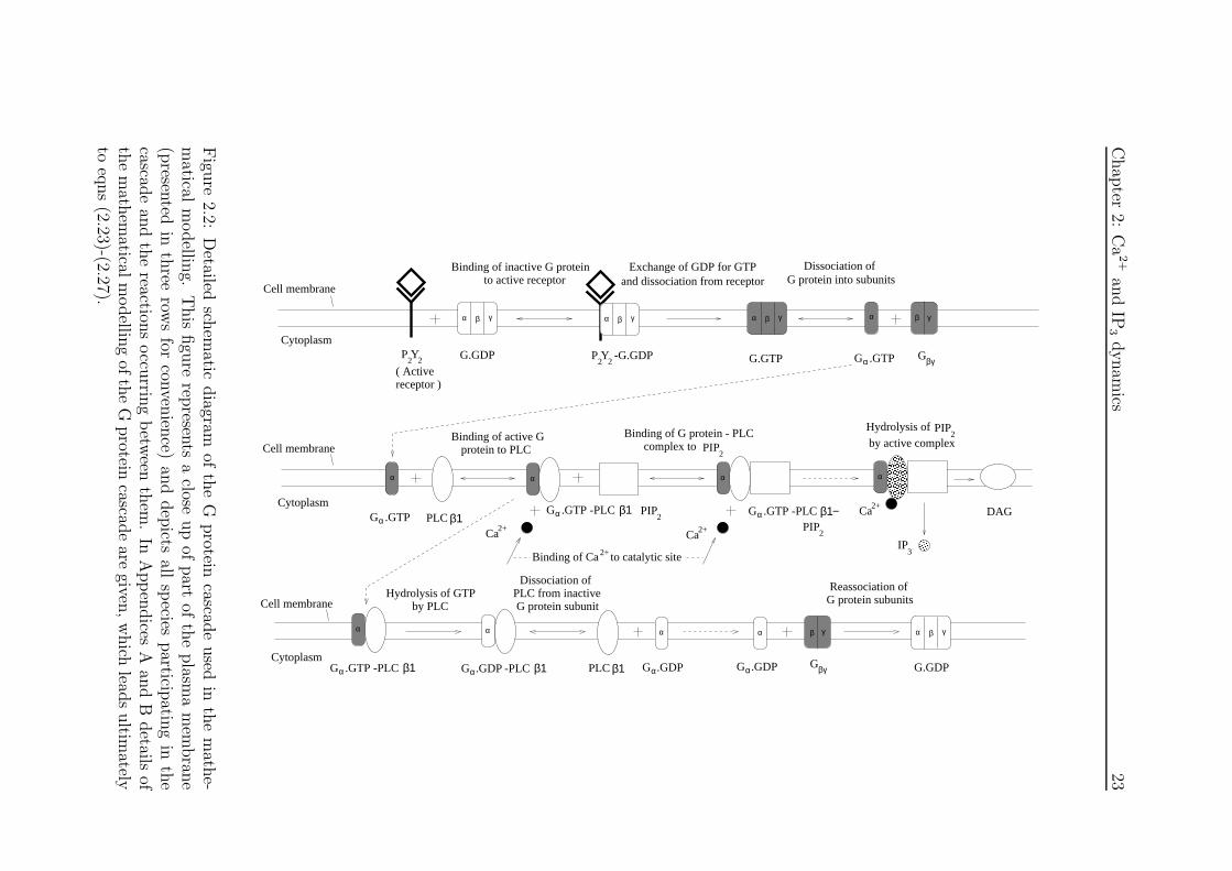
2.2 Detailed schematic diagram of the G protein cascade used in the math-
ematical modelling . . . . . . . . . . . . . . . . . . . . . . . . . . . . . 23
2.3 Experimental and theoretical numbers of surface receptors, (a) as a func-
tion of ligand concentration and (b) as a function of time following a step
application of 1 mM UTP . . . . . . . . . . . . . . . . . . . . . . . . . 32
2.4 Variations in the real parts of the eigenvalues of eqns (2.13) and (2.14)
with respect to ligand concentration . . . . . . . . . . . . . . . . . . . . 33
viii

2.5 Theoretical cytosolic IP3 and Ca2+ concentrations and amounts of PIP2
and Gα ·GTP as functions of time for a step application of 1 mM of UTP 34
2.6 Variations in (a) peak and (b) steady-state values of IP3 concentration
with respect to ligand concentration . . . . . . . . . . . . . . . . . . . . 35
2.7 Examples of Ca2+ concentration transients used for constructing activa-
tion and desensitization curves . . . . . . . . . . . . . . . . . . . . . . . 37
Chapter 3
3.1 Schematic diagram of the GFP-PHD system . . . . . . . . . . . . . . . 50
3.2 Summary of the reactions occurring in the membrane and in the cytosol
and the translocation of GFP-PHD between the two regions . . . . . . 52
3.3 The equilibrium relative change in fluorescence as a function of IP3 con-
centration in a single cell . . . . . . . . . . . . . . . . . . . . . . . . . . 61
3.4 The time course of experimental and theoretical fluorescence data . . . 62
3.5 Theoretical relative fluoresence changes with respect to time for the first
5 seconds after a step application of 3 µM ATP . . . . . . . . . . . . . 63
3.6 Peak (a) and steady-state (b) IP3 concentrations as functions of ligand
concentration . . . . . . . . . . . . . . . . . . . . . . . . . . . . . . . . 66
3.7 Experimental and theoretical maximum change in relative fluorescence
as functions of applied ligand concentration . . . . . . . . . . . . . . . 67
Chapter 4
4.1 Schematic diagram of the intracellular space through which the Ca2+
waves propagate . . . . . . . . . . . . . . . . . . . . . . . . . . . . . . . 76
4.2 Bifurcation diagrams of the channel parameter α with respect to channel
firing time difference ∆ for different domain widths, w . . . . . . . . . 84
4.3 Bifurcation diagrams of α with respect to ∆ for different domain heights,
h . . . . . . . . . . . . . . . . . . . . . . . . . . . . . . . . . . . . . . . 85
4.4 Figure showing the variations in wave speed and channel parameter crit-
ical value, αc, with domain height . . . . . . . . . . . . . . . . . . . . . 86
ix
4.5 (a) Ca2+ wavefront profiles for α = 0.25, h = 0.1 and w = 10 in the
absence of Ca2+ pumps, (b) corresponding time courses of Ca2+ concen-
tration . . . . . . . . . . . . . . . . . . . . . . . . . . . . . . . . . . . . 88
4.6 Ca2+ concentration, c, with respect to x and z on the plane y = 0 in the
presence of SR Ca2+ pumps . . . . . . . . . . . . . . . . . . . . . . . . 89
4.7 Bifurcation diagram of α with respect to ∆ for different values of the
SR pump rate, γsr . . . . . . . . . . . . . . . . . . . . . . . . . . . . . 91
4.8 Bifurcation diagrams of α with respect to ∆ in the presence of SR pumps
for different domain heights, h . . . . . . . . . . . . . . . . . . . . . . . 92
4.9 Bifurcation diagrams of α with respect to ∆ for different arrangements
of the SR and SL pumps . . . . . . . . . . . . . . . . . . . . . . . . . . 93
4.10 (a) Bifurcation diagrams of α with respect to ∆ for different values of
the channel opening time, τ , (b) wavefront profiles for the case τ = 1
and α = 0.01 . . . . . . . . . . . . . . . . . . . . . . . . . . . . . . . . 96
x
List of Tables
Chapter 2
2.1 Model parameter values used in Chapter 2 . . . . . . . . . . . . . . . . 41
Chapter 3
3.1 Model parameter values used in Chapter 3 . . . . . . . . . . . . . . . . 70
xi
List of Abbreviations Used
ATP adenosine triphosphate
Ca2+ calcium
CICR Ca2+ induced Ca2+ release
EC excitation-contraction
ER endoplasmic reticulum
FDF fire-diffuse-fire
GFP green fluorescent protein
GFP-PHD green fluorescent protein-pleckstrin homology domain
GP green fluorescent protein (abbreviation of GFP)
IICR IP3 induced Ca2+ release
IP3 inositol 1,4,5-trisphosphate
MDCK Madin-Darby canine kidney
NA noradrenaline
PHD pleckstrin homology domain
PIP2 phosphatidylinositol 4,5-bisphosphate
PLC phospholipase C
SERCA sarcoplasmic/endoplasmic reticulum Ca2+ ATPase
SL sarcolemma
SR sarcoplasmic reticulum
STOC spontaneous transient outward current
UTP uridine triphosphate
xii

1
Chapter 1
Introduction
This thesis contains a theoretical investigation of three different but related topics
relating to intracellular second messenger signalling in isolated cells. These topics are
addressed in the three subsequent chapters. In the present chapter, the background
will be given for each topic and the scope of this thesis placed in the broader context
of the study of cell physiology.
1.1 Intracellular signal transduction
The behaviour of a cell can be modified by signals from its external environment in a
number of different ways. Chemical signals can enter a cell by their being passively or
actively transported through the cell membrane, by being endocytosed in vesicles, or
by diffusing through gap junctions. They can also act directly on receptor molecules
in the cell membrane which can in turn trigger a cascade of events inside the cell.
These receptor activating ‘primary’ messenger chemicals fall into three broad functional
groups, (1) those that elicit a specific physiological response, for example an action
potential, muscle contraction or chemotaxis; (2) those that alter gene expression, that
is, change the way protein manufacture is specified by the nucleus; and (3) those that
stimulate the proliferation of cells, that is, change the rate of cell division.
Receptors belong to one of two subtypes, the ionotropic receptors or the metabotropic
receptors. Ionotropic receptors are ligand gated ion channels in the cell membrane, an
example being the NMDA receptor which plays a vital role in the generation of post
synaptic action potentials in neurons. In contrast, metabotropic receptors relay the
primary messenger stimulus by bringing about the generation of secondary signalling
molecules, or ‘second messengers’ inside the cell (Fig. 1.1). The most important second
Chapter 1: Introduction 2
messengers are cyclic AMP (cAMP) and calcium (Ca2+), both of which have a diverse
range of targets within cells. cAMP is involved in signalling pathways controlling cell
division and gene expression. Ca2+ plays a vital role in subcellular processes such as
vesicle secretion, membrane excitability and muscle contraction. It can also cause cell
death (apoptosis) in the case where there is an abnormally high mitochondrial Ca2+
concentration (Berridge et al., 1998).
A process common to many cell types by which metabotropic receptor activation re-
leases intracellular Ca2+ is where the receptors activate G-proteins which then acti-
vate the enzyme phospholipase C (PLC). PLC breaks down the membrane lipid phos-
phatidylinositol 4,5-bisphosphate (PIP2) leading to the formation of the intermediate
second messenger, inositol 1,4,5-trisphosphate (IP3) (Berridge, 1993). IP3 diffuses from
the membrane into the cell and acts on receptors located on internal stores of Ca2+, the
endoplasmic reticulum (ER) or sarcoplasmic reticulum (SR) in the case of myocytes
(contractile cells), leading to an increase in Ca2+ concentration in the cell. Release
of Ca2+ from the ER/SR is due to two main receptor types, the IP3 channel and the
ryanodine channel (so called because of its high sensitivity to the plant alkaloid ryan-
odine). The IP3 sensitive channel opens upon binding of both IP3 and Ca2+ and hence
is said to exhibit both IP3 induced Ca2+ release (IICR) and Ca2+ induced Ca2+ release
(CICR). However, the ryanodine channel is insensitive to IP3 and exhibits only CICR.
Despite the important role of metabotropic receptor pathways in the Ca2+ dynamics of
cells, there is at present no complete theoretical model for the complete process leading
from receptor activation through to intracellular Ca2+ release. One of the aims of this
thesis is to address this need and in Chapter 2 a mathematical model is developed
which incorporates realistic modelling for the different parts of the signalling pathway.
Features such as internalization and desensitization of receptors, depletion of PIP2,
activation of PLC by Ca2+, realistic IP3 channel characteristics and buffering of Ca2+
are all included, being factors likely to affect the time course of intracellular Ca2+ and
IP3 concentration upon application of agonist. As discussed in Chapter 2, CICR due
to ryanodine receptors is assumed to be negligible and is not included in the modelling.
Except where otherwise stated, exchange of ions through channels in the cell membrane
is also neglected.
In deriving the model, the various chemical species are assumed to be distributed uni-
formly in the cell membrane and cytosol. The resulting mathematical model is in the
form of a set of non-linear ordinary differential equations (ODEs) containing a number
of undetermined parameters. Values for these parameters are obtained when consider-
ation of the model is given with regard to data of in vitro experiments conducted on

Chapter 1: Introduction 3
specific cell systems.
There are many different types of G protein coupled membrane receptors to which such
a model could be applicable. This thesis, however, is concerned with the P2Y2 recep-
tor, a member of the P2 class of receptors (reviewed by Harden et al., 1995), which
binds purinergic ligands such as adenosine triphosphate (ATP) and uridine triphos-
phate (UTP). The P2Y2 receptor is present in a wide variety of different cell types and
the regulation of intracellular Ca2+ in which it plays a role has many purposes. For
example, activation of P2Y2 receptors by UTP in airway epithelial cells increases Ca2+
activated chloride ion secretion through the cell membrane, and may form the basis of
improved therapies for cystic fibrosis (Knowles et al., 1991).
The P2Y2 receptor is present in the membrane of the 1321N1 human astrocytoma cells
(Garrad et al., 1998) to which application of the model is given in Chapter 2, and is
also expressed in Madin-Darby canine kidney (MDCK) epithelial cells (Hirose et al.,
1999), to which the model is applied to in Chapter 3. Where possible, parameter values
were obtained from previously published data. Other parameter values were obtained
by adjusting the parameters so that the theoretical predictions of the model fitted the
experimental results.
Quantifying the relationships between chemical species in the form of a mathematical
model and applying it to real experimental data is important for several reasons. For
example, the model predictions can be compared with experimental results to validate
and refine the theory on which the modelling is based. It can also allow predictions to
be made about unknown quantities in an experiment, such as species concentrations
and values of parameters. Also, the modelling can sometimes uncover interesting rela-
tionships between quantities, such as that between the rate of PIP2 depletion and time
course of Ca2+ and IP3 concentration in cells which is a key finding of this thesis.
In vivo, different ligands may simultaneously act on a cell (see Fig. 1.1, A). For example
both noradrenaline (NA) and ATP are cotransmitters released at the neuromuscular
junction causing contraction of rat tail artery smooth muscle cells (Stjarne and Stjarne,
1995). Also, the same kind of ligand can act on more than one type of receptor, to
liberate intracellular Ca2+ through multiple signalling pathways (Fig. 1.1, B). In the
previous example, NA acts simultaneously on the α1 and α2 adrenergic G-protein
coupled receptors bringing about contraction through IICR. In some cases, the same
type of receptor can work by simultaneously activating different intracellular pathways
(Fig. 1.1, C). For example, during fertilization of sea urchin eggs, internal Ca2+ is mo-
bilized due to the production of the second messengers IP3, adenosine diphosphoribose
(cADPR) and nicotinic acid adenine dinucleotide phosphate (NAADP+) (Da Silva and
Chapter 1: Introduction 4
Guse, 2000). As discussed in Chapter 2 the P2Y2 receptor can activate distinct path-
ways comprising different G-protein and PLC species, albeit to release the same second
messenger, IP3.
The reasons for multiple signalling pathways for the same primary messenger is be-
lieved to include (a) the need for the safety of having built-in redundancy, (b) the
provision of Ca2+ responses of different amplitude and duration for the fine tuning of
the physiological response; and (c) the need to ensure localized Ca2+ release by spa-
tial localization of molecules constituting the different signalling pathways (Da Silva
and Guse, 2000). Point (b) appears to be the case for the rat tail artery where ATP
and NA mediate a biphasic contractile response with the former contributing a rapid
‘phasic’ response and the latter a slow ‘tonic’ response. Point (c) may be true of the
P2Y2 receptor, which is in some cases localized in patches on the cell membrane (see
Fig. 1.2, also Sromek and Harden, (1998); Fig. 6A). PIP2 has also been shown to
be localized in caveolae, small flask shaped infoldings of the plasma membrane 70-100
nm in diameter, which indicates that IP3 production may be heterogeneous in the cell
membrane (Pike and Casey, 1996). Spatial localization of receptors and PIP2 in non-
overlapping domains would suggest the importance of membrane diffusion of PLC and
G-protein molecules to provide signal coupling across the membrane.
In Chapter 2 discussion is given of how the mathematical model developed in that
chapter could be extended to include the more detailed aspects of signalling pathways
described above.
Chapter 1: Introduction 5
���������������
���������������
Second messengers
Ca2+
cellmembrane
A
B
Ligand
C
Receptor
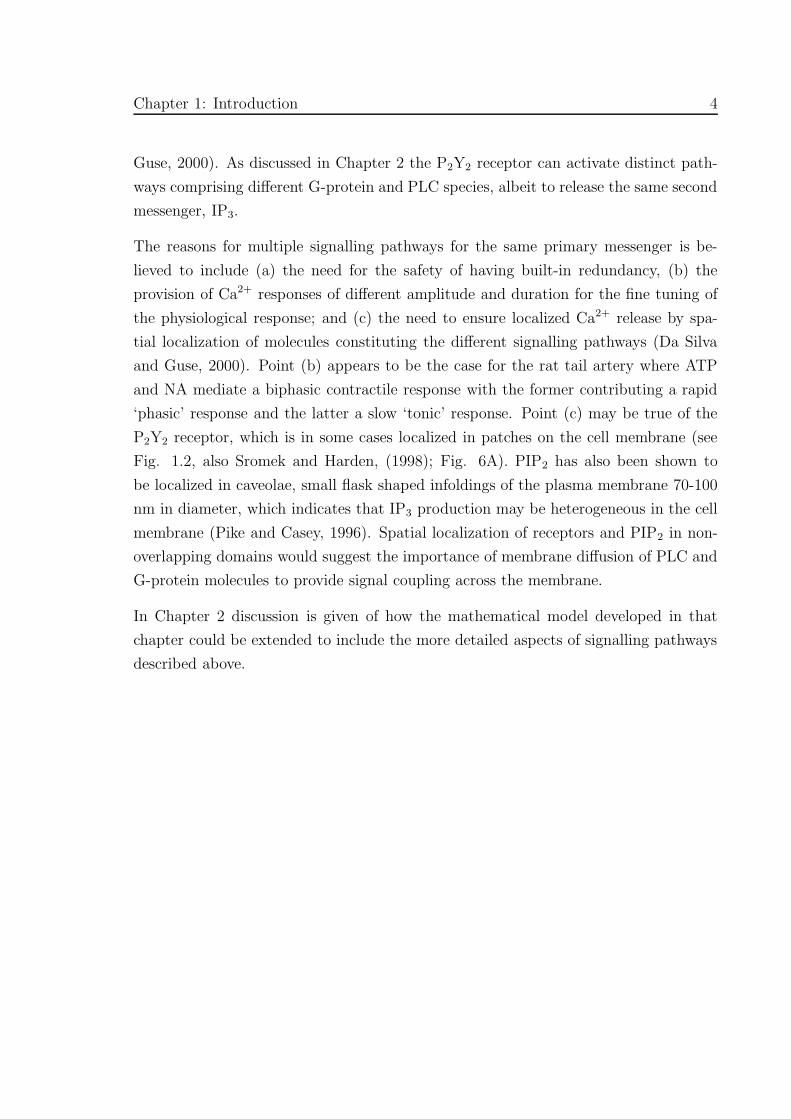
Figure 1.1: Schematic diagram of intracellular release of Ca2+ inside a cell mediated byother second messengers (filled circles) (A) due to the different extracellular primarymessengers (ligands) working through different receptors, (B) due to the same pri-mary messenger working through different receptors and (C) due to the same primarymessenger and receptor working through different intracellular pathways.
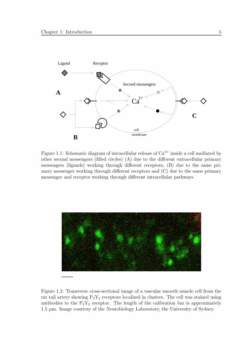
Figure 1.2: Transverse cross-sectional image of a vascular smooth muscle cell from therat tail artery showing P2Y2 receptors localized in clusters. The cell was stained usingantibodies to the P2Y2 receptor. The length of the calibration bar is approximately1.5 µm. Image courtesy of the Neurobiology Laboratory, the University of Sydney.
Chapter 1: Introduction 6
1.2 Fluorescent indicators in cell biology
Fluorescent indicators play an important role in the experimental study of cell pro-
cesses. A fluorescent probe molecule introduced into a cell may preferentially bind to
some other molecule inside the cell, or if it is transfected into the cell (written into the
cells genome), may be expressed preferrentally in certain parts of the cell. Using opti-
cal microscopy techniques, the presence and spatial location of intracellular molecules
and organelles can then be visualized. A probe that is proving highly useful for this
procedure is the green fluorescent protein (GFP), a protein occurring naturally in the
jellyfish Aequorea victoria (reviewed in Tsien, 1998). For example, GFP attached to
sarcoplasmic/endoplasmic reticulum Ca2+-ATPase proteins (SERCA) has been used
to visualize the dynamics of SERCA molecules in the endoplasmic reticulum and the
alveolar sacs of Paramecium cells (Hauser et al., 2000). Similar results may come
from studying the tissues of ANDi, a transgenic rhesus monkey created by infecting
unfertilized eggs with the gene for GFP (Chan et al., 2001).
The fluorescence or (photon) absorption properties of some probes change upon binding
with ions such as Ca2+, for a review see Tsien (1989). Some examples of Ca2+ sensitive
probes are fura-2, which exhibits a shift in absorbance spectra to shorter wavelengths
upon binding of Ca2+, and fluo-3 where Ca2+ binding results in an increase in efficiency
of fluorescence. This effect is widely used by experimentalists to image spatial and
temporal changes in Ca2+ concentration within live cells. The probes are introduced
into the cell by micro-injection or by being permeable to the cell membrane. Optical
microscopy techniques can then be used to image the probe. Confocal microscopes are
useful for obtaining plane cross-sectional images of probe distributions in cells.
The chemical properties of the probe can have a significant effect on the dynamics of
intracellular Ca2+. If the concentration of the probe is large relative to the amount of
free Ca2+, significant amounts of Ca2+ maybe bound to the indicator thereby critically
altering the supply of Ca2+ in the cytosol. The binding of Ca2+ to a probe slows the
rate of diffusion of Ca2+ (Wagner and Keizer, 1994) in the same way as endogenous
buffers (hence Ca2+ indicators are frequently referred to as ‘buffers’). Saturation of the
binding of Ca2+ with the probe and the slow rate of binding relative to fast intracel-
lular Ca2+ events, for example Ca2+ sparks, also affects the relation between the Ca2+
concentration and the indicator response. Therefore it is often necessary to include the
presence of the Ca2+ indicators in the modelling as has been done in Chapter 2, see
also Smith et al. (1998) for a study of the effects of Ca2+ buffers on sparks. However,
the concentration of the indicator within a cell is usually not known precisely and esti-
mates or typical values are often used. The inexactness of measuring the concentration
Chapter 1: Introduction 7
of the Ca2+ indicator is a problem particularly with probes such as fluo-3 where the
dependence of fluorescence on Ca2+ concentration depends on the concentration of the
indicator.
This thesis makes much use of experimental data where fluorescent probes for Ca2+
have been used. In Chapters 2 and 3 measurements of Ca2+ concentrations expressed
as molar quantities were obtained from experiments that used fura-2. In Chapter 4,
the experimental data of images of Ca2+ sparks used fluo-4.
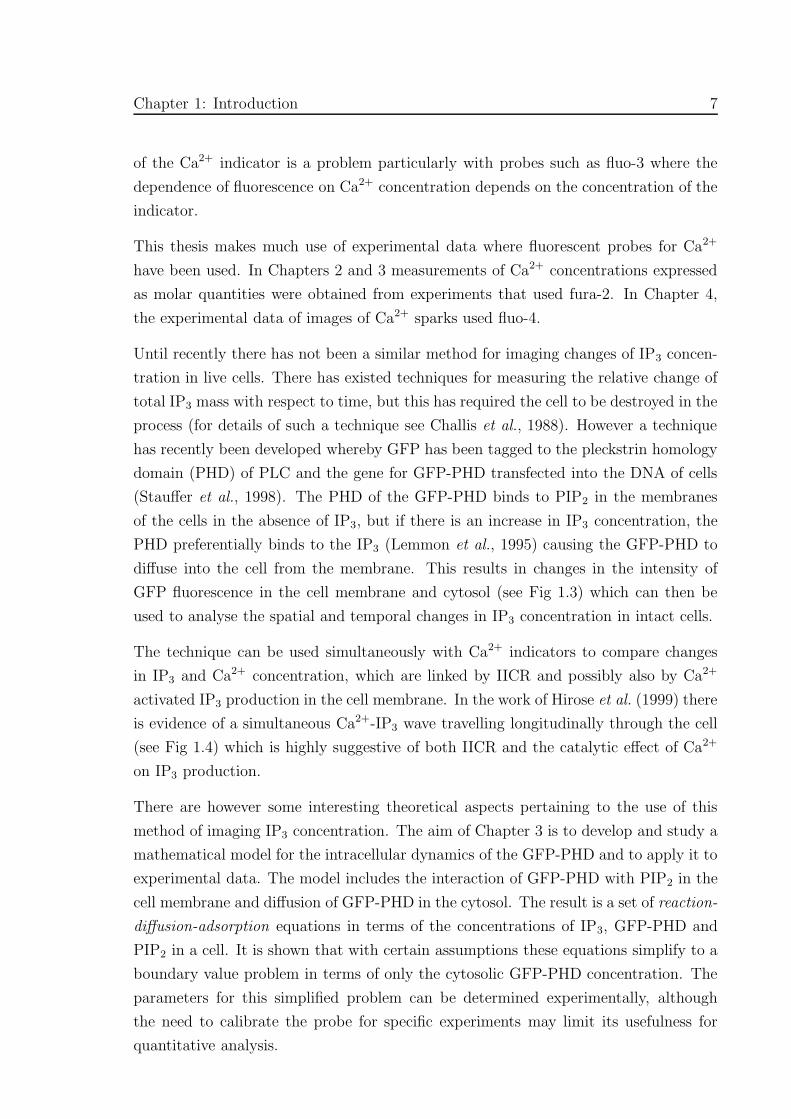
Until recently there has not been a similar method for imaging changes of IP3 concen-
tration in live cells. There has existed techniques for measuring the relative change of
total IP3 mass with respect to time, but this has required the cell to be destroyed in the
process (for details of such a technique see Challis et al., 1988). However a technique
has recently been developed whereby GFP has been tagged to the pleckstrin homology
domain (PHD) of PLC and the gene for GFP-PHD transfected into the DNA of cells
(Stauffer et al., 1998). The PHD of the GFP-PHD binds to PIP2 in the membranes
of the cells in the absence of IP3, but if there is an increase in IP3 concentration, the
PHD preferentially binds to the IP3 (Lemmon et al., 1995) causing the GFP-PHD to
diffuse into the cell from the membrane. This results in changes in the intensity of
GFP fluorescence in the cell membrane and cytosol (see Fig 1.3) which can then be
used to analyse the spatial and temporal changes in IP3 concentration in intact cells.
The technique can be used simultaneously with Ca2+ indicators to compare changes
in IP3 and Ca2+ concentration, which are linked by IICR and possibly also by Ca2+
activated IP3 production in the cell membrane. In the work of Hirose et al. (1999) there
is evidence of a simultaneous Ca2+-IP3 wave travelling longitudinally through the cell
(see Fig 1.4) which is highly suggestive of both IICR and the catalytic effect of Ca2+
on IP3 production.
There are however some interesting theoretical aspects pertaining to the use of this
method of imaging IP3 concentration. The aim of Chapter 3 is to develop and study a
mathematical model for the intracellular dynamics of the GFP-PHD and to apply it to
experimental data. The model includes the interaction of GFP-PHD with PIP2 in the
cell membrane and diffusion of GFP-PHD in the cytosol. The result is a set of reaction-
diffusion-adsorption equations in terms of the concentrations of IP3, GFP-PHD and
PIP2 in a cell. It is shown that with certain assumptions these equations simplify to a
boundary value problem in terms of only the cytosolic GFP-PHD concentration. The
parameters for this simplified problem can be determined experimentally, although
the need to calibrate the probe for specific experiments may limit its usefulness for
quantitative analysis.

Chapter 1: Introduction 8
Solution of the simplified equations for the case of cylindrical and circular cells reveals
the presence of a delay in the diffusing of GFP-PHD between the membrane and
cytosol. Also the modelling reveals that PIP2 depletion causes translocation of GFP-
PHD to the cytosol. This complicates the relation between GFP-PHD fluorescence and
IP3 concentration in cases where there is significant depression of PIP2 levels during
agonist stimulation.
In Chapter 3 the model for the dynamics of the GFP-PHD is also used in conjunction
with the complete cell model given in Chapter 2, to quantify Ca2+ and GFP-PHD
fluorescence data for the purinergic stimulation of MDCK cells with ATP (Hirose et
al., 1999).
Chapter 1: Introduction 9
t = 0 t ≈ 1min t ≈ 2min t ≈ 3min t ≈ 4min
Figure 1.3: Sequential images showing the time variations of GFP-PHD fluorescencein a smooth muscle cell exposed to ATP at t = 0. The reduction of fluorescenceintensity over time on parts of the cell membrane is evidence of the translocationof GFP-PHD from these areas due to the presence of IP3 or PIP2 depletion. Theretention of membrane GFP-PHD seen at the end regions of the cell could be due totrapping of GFP-PHD by peripheral SR or preferential trafficking of PIP2 to theseregions. The length of the calibration bar is approximately 1 µm. Images courtesy ofthe Neurobiology Laboratory, the University of Sydney.

Chapter 1: Introduction 10
Figure 1.4: Images showing the intracellular dynamics of Ca2+ and IP3 in an MDCKepithelial cell. The time courses of the signals from the regions indicated by the num-bered boxes are plotted. The presence of a simultaneous Ca2+-IP3 wave is indicated bythe elevation of GFP-PHD fluorescence simultaneously with Ca2+ concentration. Thisfigure is taken from Fig. 4 of Hirose et al. (1999).

Chapter 1: Introduction 11
The use of the GFP-PHD as a probe for IP3 is receiving increasing interest by ex-
perimentalists. It is envisaged that the modelling techniques and results contained in
Chapter 3 will prove useful in future application of the GFP-PHD probe in experi-
ments. Indeed, at the time this thesis was in the final stages of completion, a paper
was published (Xu et al., 2003) detailing an experimental and mathematical modelling
study of bradykinin induced changes in N1E-115 neuroblastoma cells. The study con-
tains an independently devised model for the GFP-PHD dynamics and also includes
a simple mathematical model for phosphoinositide turnover in the membrane of these
cells. The results of that paper show agreement with the time course of PIP2 recovery
after treatment with agonist predicted in Chapter 2 and also that both IP3 generation
and PIP2 depletion cause translocation of GFP-PHD to the cytosol.
1.3 Intracellular Ca2+ waves
The experimental data used in Chapters 2 and 3, namely that of the purinergic stimu-
lation of 1321N1 cells and MDCK cells, exhibits a Ca2+ and IP3 response that increases
over a period of tens of seconds, and decreases over a period of several minutes. Over
these time scales, the concentration of Ca2+ and IP3 can be assumed to be homoge-
neous through the cytosol, assuming that the processes in the model are not spatially
dependent. Under these assumptions there is no need to incorporate diffusion of Ca2+
or IP3 into the model. In some cases however, evidence shows that there is distinc-
tive heterogeneity in the release of intracellular Ca2+. This heterogeneity can take the
form of Ca2+ wave fronts propagating through the cell or spontaneous, highly localized
releases of Ca2+ called ‘sparks’.
Ca2+ waves usually occur when Ca2+ is released from Ca2+ sensitive ion channels
located in the ER/SR. Typically the spatial extent of the wave front is much longer
than the characteristic distance between the release channels. In this limit, Ca2+
release into the cytosol can be assumed to occur from channels distributed continuously
through the ER/SR. The fine structure of the ER/SR, which is believed to be a network
of interconnected tubules, is usually ignored in modelling studies and assumed to be
a continuum. However, there is evidence that the ER/SR can comprise spatially and
functionally distinct parts (Golovina and Blaustein, 1997). In some cells the peripheral
ER/SR, which is located close to the cell membrane, becomes effectively a barrier
between the cell membrane and the bulk of the cell. The dynamics of Ca2+ in the space
between the peripheral ER/SR and the cell membrane, called the ‘subsarcolemmal’
space in the case of myocytes, differs from that in the bulk of the cell. Thus the

Chapter 1: Introduction 12
character of the Ca2+ waves in these peripheral regions will be quite different from
those in the central part. For example in the rat megakaryocyte (Thomas et al., 2001)
and Xenopus laevis egg (Fontanilla and Nuccitelli, 1998), Ca2+ waves in the peripheral
parts of the cell are observed to travel with a greater speed than those in the central
part.
In essence, intracellular Ca2+ waves arise from the non-linear relation between Ca2+
concentration and Ca2+ channel current coupled to diffusion of Ca2+ in the cytosol.
However, modelling studies show that wave propagation can also depend on the inter-
play of a variety of factors such as the presence of SERCA and cell membrane pumps,
ER/SR leaks and cytosolic Ca2+ buffering (Jafri and Keizer, 1995). Ca2+ waves are im-
portant physiologically because they allow small, localized increases of cytosolic Ca2+
to trigger global release of Ca2+ through the cell.
Mathematical models of systems exhibiting Ca2+ waves typically comprise sets of cou-
pled reaction-diffusion equations. Although strictly speaking cell systems always have
three space dimensions, the dominant mode of propagation often has fewer dimen-
sions. For example in long thin cells such as myocytes, Ca2+ concentration equilibrates
rapidly in the transverse direction and so wave propagation can be modelled in only
the longitudinal direction. In spherically shaped cells such as Oocytes, fertilization
Ca2+ wavefronts observed in the equatorial plane viewed under a confocal microscope
appear planar, warranting the use of a model with two space dimensions (Wagner et
al., 1998).
The other type of heterogeneity of intracellular release, that of ‘sparks’ of Ca2+, results
from the release of Ca2+ from discrete openings of clusters of ryanodine sensitive chan-
nels located in the ER/SR. Discrete openings of clusters of IP3 sensitive channels can
also occur in some cases, causing localized release of Ca2+ called ‘puffs’ (Parker and
Yao, 1991). Ca2+ sparks can occur spontaneously but their probability also exhibits
dependence on Ca2+ concentration owing to their CICR properties (Gyorke and Fill,
1993). The spontaneous nature of sparks is evident in whole cell Ca2+ measurements
which take on a spiky, noise-like appearance due to contributions by sparks at different
sites within the cell (see Fig 1.5). Whereas the locations of the sites of sparks may
be anywhere inside a cell, the occurrence of sparks near the cell membrane can be of
special physiological significance. In smooth muscle, sparks near the cell membrane
open large conductivity Ca2+ sensitive potassium (BK) channels which brings about
spontaneous transient outward currents (STOCs). These are thought to provide a neg-
ative feedback mechanism for contraction by hyperpolarizing the cell membrane and
thereby reducing activated Ca2+ entry through voltage gated L-type Ca2+ channels in
Chapter 1: Introduction 13
the membrane (Jaggar et al., 2000).
In cardiac cells, Ca2+ sparks play an important role in excitation-contraction (EC)
coupling whereby an action potential induces contraction of the cell. The main means
of electrical coupling between cardiac cells are gap junctions (Severs, 1995) which
connect the cytoplasms of adjacent cells and permit the exchange of small molecules
(< 1 kDa) between them. These allow intercellular waves arising from the sinoatrial
node (the pacemaker of the heart) to propagate through the heart tissue. Thus the
‘primary message’ to bring about contraction in cardiac muscle is communicated via
gap junctions, whereas in smooth muscle tissue the signal is communicated by both
gap junctions and neurotransmitter, which is released from varicosities on the cells and
activates metabotropic and ionotropic receptors. The depolarization of the membrane
of the myocyte which occurs during an action potential triggers Ca2+ influx through
voltage gated L-type channels in the sarcolemma (SL) which in turn triggers Ca2+
sparks. Unlike in smooth muscle, the dominant mode of intracellular Ca2+ release in
cardiac cells is CICR through ryanodine channels.
Ventricular myocytes have infoldings in the SL known as T-tubules, which allows an
action potential to propagate (speed of the order 1×104 µm.(ms)−1) deep inside the
cell. This activates sparks inside the dyadic cleft, which is the space between the
SL at the end of the T-tubule and sarcoplasmic reticulum. T-tubules are thought to
allow rapid release of intracellular Ca2+ and concomitant cell contraction, bypassing
the need for Ca2+ to be released by way of a radially propagating Ca2+ wave which is
far slower (of the order 0.1 µm.(ms)−1) (Brette and Orchard, 2003). Atrial myocytes,
like other cardiac cells such as pacemaker and Purkinje cells, do not possess T-tubules
but appear to have structures homologous to dyadic clefts, where the SR and SL are
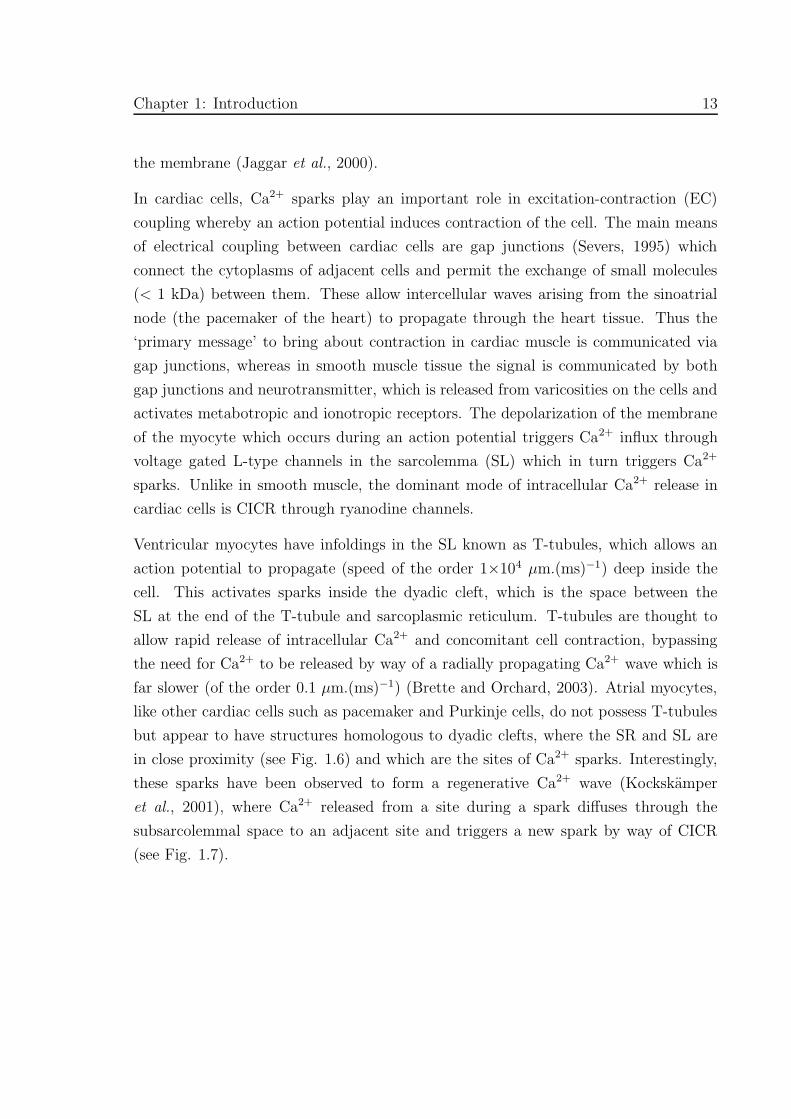
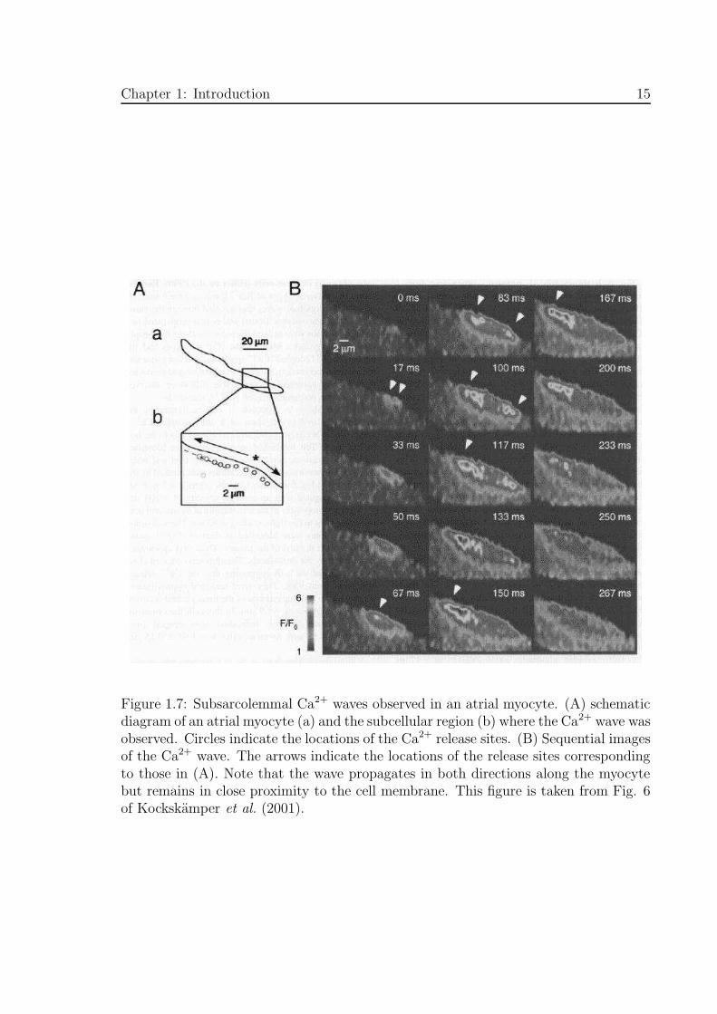
in close proximity (see Fig. 1.6) and which are the sites of Ca2+ sparks. Interestingly,
these sparks have been observed to form a regenerative Ca2+ wave (Kockskamper
et al., 2001), where Ca2+ released from a site during a spark diffuses through the
subsarcolemmal space to an adjacent site and triggers a new spark by way of CICR
(see Fig. 1.7).

Chapter 1: Introduction 14
Figure 1.5: Time course of global Ca2+ in a tracheal smooth muscle cell revealing atrain of Ca2+ sparks. This figure is taken from Fig. 7 of Pabelick et al. (1999), for thecase of no extracellular Ca2+.
∨ ∨
Figure 1.6: Electron micrograph of a longitudinally cut atrial myocyte. The locationsof two peripheral couplings are marked by arrows. The length of the calibration bar is200 nm. This figure is taken from Fig. 9 of Kockskamper et al. (2001).
Chapter 1: Introduction 15
Figure 1.7: Subsarcolemmal Ca2+ waves observed in an atrial myocyte. (A) schematicdiagram of an atrial myocyte (a) and the subcellular region (b) where the Ca2+ wave wasobserved. Circles indicate the locations of the Ca2+ release sites. (B) Sequential imagesof the Ca2+ wave. The arrows indicate the locations of the release sites correspondingto those in (A). Note that the wave propagates in both directions along the myocytebut remains in close proximity to the cell membrane. This figure is taken from Fig. 6of Kockskamper et al. (2001).

Chapter 1: Introduction 16
A mathematical model for these subsarcolemmal Ca2+ waves is developed and analysed
in Chapter 4, using an adaptation of the so called fire-diffuse-fire (FDF) model for
Ca2+ waves (Keizer et al., 1998; Keizer and Smith, 1998). Various simplifications are
made in the modelling, for example despite the highly non-uniform dimensions of the
subsarcolemmal region (see Fig. 1.6) the domain is modelled as a perfectly rectangular
space, infinite in extent in the direction of propagation (see Fig. 4.1). Also, the Ca2+
pump rate for pumps in the SR and SL, and the amount of Ca2+ bound to buffers is
assumed to depend linearly on Ca2+ concentration. This approach to the modelling
differs from that taken in Chapters 2 and 3, where all aspects of the model were
treated as realistically as possible. Nevertheless, this allows analytic solutions to be
obtained for the Ca2+ concentration due to a spark, whereas solution of a fully non-
linear reaction-diffusion formulation on a domain of infinite extent would be highly
problematic.
The ease of computation of solutions to the model equations facilitates the compre-
hensive bifurcation analysis of the solutions given in Chapter 4. This contrasts with
the approach taken in Chapters 2 and 3 where the main aim was to determine specific
parameter values for the model equations from experimental data. This bifurcation
analysis of the solutions of the model equations shows how the existence, stability and
speed of these restricted Ca2+ waves depend critically on the values of the model pa-
rameters. It is likely that these results will carry over into computational studies that
use more realistic modelling such as a more detailed geometry of the subsarcolemmal
space. It is plausible that atrial myocytes make use of the confined subsarcolemmal
space to amplify, direct and hasten intracellular Ca2+ release longitudinally through
the cell during the EC process.
It is interesting to ask whether in some cells peripheral membranes can trap IP3 pro-
duced in the membrane and restrict its diffusion into the central parts of the cell.
This question could perhaps be answered using the GFP-PHD technique discussed in
Chapter 3, to image IP3 concentrations in these restricted domains.
Chapter 1: Introduction 17
Although the model applies to Ca2+ waves in the subsarcolemmal regions of cells
specifically atrial myocytes (Kockskamper et al., 2001), the results show more generally
how the nature of the cell in the vicinity of the release site may have a significant
effect on the Ca2+ released in a propagating wavefront. For example, in some cells
Ca2+ release might be confined by the tortuous nature of the ER/SR or by other
intracellular organelles such as mitochondria. Therefore, even for continuum models
of Ca2+ waves using a reaction-diffusion formulation, it may not be appropriate to use
reaction terms based solely on the properties of ion channels that have been isolated
in lipid membranes.

18
Chapter 2
Modelling calcium and inositol1,4,5-trisphosphate dynamicsfollowing receptor activation
In this chapter, a mathematical account is given of the processes governing the time
courses of calcium ions (Ca2+), inositol 1,4,5-trisphosphate (IP3) and phosphatidylinos-
itol 4,5-bisphosphate (PIP2) in single cells following the application of external agonist
to metabotropic receptors. A model is constructed that incorporates the regulation of
metabotropic receptor activity, the G protein cascade and the Ca2+ dynamics in the cy-
tosol. It is subsequently used to reproduce observations on the extent of desensitization
and sequestration of the P2Y2 receptor following its activation by uridine triphosphate
(UTP). The theory predicts the dependence on agonist concentration of the change
in the number of receptors in the membrane as well as the time course of disappear-
ance of receptors from the plasmalemma, upon exposure to agonist. In addition, the
extent of activation and desensitization of the receptor, using the Ca2+ transients in
cells initiated by exposure to agonist, is also predicted. Model predictions show the
significance of membrane PIP2 depletion and resupply on the time course of IP3 and
Ca2+ levels. Results of the modelling also reveal the importance of receptor recycling
and PIP2 resupply for maintaining Ca2+ and IP3 levels during sustained application of
agonist.
2.1 Introduction
Agonist-induced activation of second messenger systems plays an important role in
the mobilization of stored Ca2+ inside cells (Berridge, 1993; Miyazaki, 1995). A first
stage in this process is the binding of a ligand to a G-protein coupled receptor, the
Chapter 2: Ca2+ and IP3 dynamics 19
metabotropic receptor. This sets off a cascade of events leading to the activation of the
enzyme phospholipase C (PLC) which hydrolyses the membrane-bound phospholipid,
phosphatidylinositol 4,5-bisphosphate (PIP2) to inositol 1,4,5-trisphosphate (IP3) and
diacylglycerol. IP3 then diffuses into the cytosol and interacts with Ca2+ channels in the
endoplasmic reticulum (ER) causing the release of stored Ca2+ (Tsien and Tsien, 1990;
Amundson and Clapham, 1993). At present there is no complete and unified model of
the processes enumerated above, starting from the binding of ligand to metabotropic
receptors and leading, via a G-protein cascade, to the production of IP3 and the release
of Ca2+ from the endoplasmic reticulum.
Although there is no comprehensive model of the events that occur after ligand binding
to metabotropic receptors, theoretical consideration has been given to various elements
of the process. A number of models have been proposed for the interactions between
receptors, ligands and G-proteins (Zigmond et al., 1982; Linderman and Lauffenburger,
1988; Lauffenburger and Linderman, 1993; French and Lauffenburger, 1997) with the
cubic ternary model (Weiss et al., 1996a,b) providing the most general description of
the interaction between the three species. Monte Carlo style simulations have also
been used to analyse the possible stochastic nature of the interactions (Mahama and
Linderman, 1994; Felber et al., 1996; Shea and Linderman, 1997). The discovery of
desensitization of receptors following phosphorylation on ligand binding with subse-
quent internalization of the receptors has prompted the inclusion of these processes in
more recent attempts to build quantitative models (Riccobene et al., 1999; Adams et
al., 1998).
Modelling the formation of IP3 by the hydrolysis of PIP2, followed by the dynamics
of Ca2+ and IP3 in the cytosol, has also been attempted. These models may include
PIP2 depletion and replenishment (Haugh et al., 2000) and also show how IP3 can
induce Ca2+ oscillations (Cutherbertson and Chay, 1991; De Young and Keizer, 1992;
Atri et al., 1993) as well as Ca2+ waves (Jafri and Keizer, 1994, 1995; Schaff et al.,
1997). With the discovery of elementary Ca2+ events, such as ‘sparks’ and ‘blips’, that
arise from the behaviour of either single ion channels or clusters of them, concentration
has centred on modelling these formations following the opening of IP3-sensitive Ca2+
channels (Smith et al., 1998; Swillens et al., 1998).
Although quantitative models of the action of hormones in inducing secretion have
recently been presented (Blum et al., 2000) there is as yet no comprehensive model of
how activation of metabotropic receptors leads to a response. Construction of such a
model involves consideration of ligand-receptor binding and its desensitization through
phosphorylation and internalization (Fig. 2.1, Box A), of the G-protein cascade leading
Chapter 2: Ca2+ and IP3 dynamics 20
to production of IP3 (Fig. 2.1, Box B) and finally of the IP3-induced Ca2+ release from
the endoplasmic reticulum (Fig. 2.1, Box C). A unified model is presented here and
used to predict observations on the results of P2Y2 receptor stimulation by ligands.
2.2 Methods
This section contains the basic equations that define the model. In order to stream-
line the presentation, additional considerations involved in constructing the model are
reserved for the Discussion section and detailed mathematical derivations are given in
Appendices A and B.
2.2.1 Regulation of metabotropic receptor activity
The regulation of metabotropic receptor activity has several components: phosphory-
lation of the receptors and their uncoupling from G-proteins; sequestration or inter-
nalization of the receptors; down-regulation of the receptors as a consequence of their
destruction in lysozomes or alternatively dephosphorylation and recycling of the recep-
tors to the membrane. The model presented here is an adaptation of that given by
Hoffman et al. (1996) for the N-formyl peptide receptor for neutrophils, the difference
being that internalized receptors are allowed to recycle to the surface. The elements of
the model are depicted in Fig. 2.1 within the box marked A, where reactions involving
ligand (L) and receptors (R) are given. Receptors on the cell surface bind extracellular
ligand reversibly, with forward and backward rate constants k+1 and k−1 , respectively.
It is assumed that ligand is not depleted by binding with receptors and hence has a
predetermined concentration.
Receptors occupied with ligand, LR, are phosphorylated irreversibly to LRP at a rate
kp but phosphorylated receptors, RP , remain free to interact with the ligand, with
possibly different binding kinetics governed by rates k±2 (Hoffman et al., 1996; Adams
et al., 1998; Riccobene et al., 1999). Phosphorylation causes desensitization of the
receptors and so G-protein may only be activated by unphosphorylated receptors (R
and LR), as indicated by the broken lines joining boxes A and B in Fig. 2.1. The
model presented here has an aspect in common with the cubic ternary complex model
(Weiss et al., 1996a,b) in that G-proteins are allowed to bind to receptors which are
both bound and unbound with ligand. However, analysis of the model as given in
Appendices A and B shows that with certain assumptions the receptor/ligand and G-
protein systems largely decouple and only the proportion of activated receptors needs

Chapter 2: Ca2+ and IP3 dynamics 21
to be specified in the G-protein cascade model.
Phosphorylated receptors are internalized at a rate that is dependent on agonist oc-
cupancy and this is incorporated into the model by having the bound phosphorylated
receptors, LRP , internalized at rate ke. These internalized receptors, RI , are then
dephosphorylated and recycled back to the surface at a rate kr.
The equations describing the processes depicted in Box A of Fig. 1 are:
d[R]
dt= −k+
1 [L][R] + k−1 [LR] + kr[RI ], (2.1)
d[LR]
dt= k+
1 [L][R] − (k−1 + kp)[LR], (2.2)
d[LRP ]
dt= k+
2 [L][RP ] − (k−2 + ke)[LRP ] + kp[LR], (2.3)
d[RP ]
dt= −k+
2 [L][RP ] + k−2 [LRP ], (2.4)
d[RI ]
dt= −kr[RI ] + ke[LRP ], (2.5)
where [L] denotes the concentration of ligand L, [R] and [LR] are the numbers of
unbound and bound receptors, [RP ] and [LRP ] are the corresponding phosphorylated
quantities and [RI ] is the number of internalized receptors. Adding eqns (2.1)-(2.5)
gives zero and so
[R] + [LR] + [LRP ] + [RP ] + [RI ] = [RT ], (2.6)
where [RT ], the total number of receptors, is a constant.
The kinetics of ligand binding are considered to be fast relative to the other processes
in the model. Eqns (2.1)-(2.5) can be combined to leave only the slow kinetics, giving
d[RS]
dt= kr[RI ] − kp[LR], (2.7)
d[RSP ]
dt= −ke[LRP ] + kp[LR], (2.8)
where [RS] = [R]+ [LR] is the total number of unphosphorylated surface receptors and
[RSP ] = [RP ] + [LRP ] is the total number of phosphorylated surface receptors.
Chapter 2: Ca2+ and IP3 dynamics 22
3IP
Ca2+
Ca2+
Ca2+Ca2+
IP3Ca2+
IP3 channel
2+
Ca2+
��
Ca
2
C
Leak
pump
Endoplasmic reticulum
PIPCytosol
B
LRL + R L + R
k
LR
R
+1
k-
A
r k
k -
k+
kk
1 2
e
p
2
p
p
I
G G PIP2
3IP
PLCR, LR
Membrane
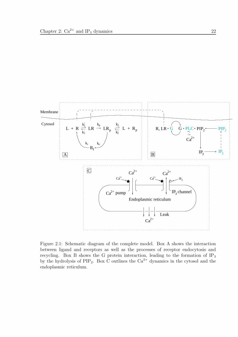
Figure 2.1: Schematic diagram of the complete model. Box A shows the interactionbetween ligand and receptors as well as the processes of receptor endocytosis andrecycling. Box B shows the G protein interaction, leading to the formation of IP3
by the hydrolysis of PIP2. Box C outlines the Ca2+ dynamics in the cytosol and theendoplasmic reticulum.
Chap
ter2:
Ca
2+
and
IP3
dynam
ics23
-PLC β1−
3
α β γ
α β γ
P Y 2 2 .GTPGα
.GTPGα.GTPGα -PLC β1 .GTPGα Ca2+
Ca2+
PLC β1.GTPGα -PLC β1 .GDPGα
Ca2+
Gβγ
Gβγ.GDPGα
G.GTPP Y 2 2
PLC β1
Binding of active Gprotein to PLC
PIP2
Hydrolysis ofby active complexPIP
2
Binding of G protein - PLCcomplex to
Binding of inactive G proteinto active receptor
Exchange of GDP for GTPand dissociation from receptor G protein into subunits
Dissociation of
Dissociation of PLC from inactiveG protein subunit
Reassociation of
by PLC G protein subunits
PIP2
� � � �� � � �� � � �� � � �� � � �� � � �� � � �� � � �� � � �� � �� � �� � �� � �� � �� � �� � �� � �� � �
� � �� � �� � �� � �� �� �� �� �
Hydrolysis of GTP
Cytoplasm
Cell membrane
2+Binding of Ca to catalytic site
2PIP
Cytoplasm
Cell membrane
( Active
Cytoplasm
Cell membrane
G.GDP
G.GDPαG
α α α
.GDP
α
β1-PLC
α α
DAG
receptor )
α
IP
-G.GDP
α
γβ
α
γβα γβ αβ γ
Figu
re2.2:
Detailed
schem
aticdiagram
ofth
eG
protein
cascade
used
inth
em
athe-
matical
modellin
g.T
his
figu
rerep
resents
aclose
up
ofpart
ofth
eplasm
am
embran
e(p
resented
inth
reerow
sfor
conven
ience)
and
dep
ictsall
species
particip
ating
inth
ecascad
ean
dth
ereaction
soccu
rring
betw
eenth
em.
InA
ppen
dices
Aan
dB
details
ofth
em
athem
aticalm
odellin
gof
the
Gprotein
cascade
aregiven
,w
hich
leads
ultim
atelyto
eqns
(2.23)-(2.27).

Chapter 2: Ca2+ and IP3 dynamics 24
Applying the rapid ligand kinetics assumption (compare the rapid buffer approxima-
tion: Wagner and Keizer, 1994) gives the following relations:
[R] =K1[R
S]
K1 + [L], (2.9)
[LR] =[L][RS ]
K1 + [L], (2.10)
[LRP ] =[L][RS
P ]
K2 + [L], (2.11)
[RP ] =K2[R
SP ]
K2 + [L], (2.12)
where K1 = k−1 /k+1 , K2 = k−2 /k
+2 . Substituting into eqns (2.7)-(2.8) and using (2.6)
gives
d[RS]
dt= kr[RT ] −
(kr +
kp[L]
K1 + [L]
)[RS] − kr[R
SP ], (2.13)
d[RSP ]
dt= [L]
(kp[R
S]
K1 + [L]− ke[R
SP ]
K2 + [L]
). (2.14)
It is likely that some fraction of the surface receptors do not recycle, perhaps through
being immobile, and are prevented from being endocytosed (see, for example, Zigmond
et al., 1982, where there is a discrepancy between the theoretical and experimental
surface receptor numbers at equilibrium.) This effect is incorporated into the present
model by supposing that a fraction ξ of receptors are mobile, so that the total number
of mobile receptors is now ξ[RT ] and the remaining receptors, numbering (1 − ξ)[RT ],
are immobile and are assumed not to participate in second-messenger signalling.
The equilibrium solution of eqns (2.13) and (2.14), that is, the solution for which the
ligand concentration has been held constant for a very long time, is found by setting
d[RS]/dt = d[RSP ]/dt = 0 and solving for [RS] and [RS
P ]. This gives the equilibrium
number of surface receptors, [RSE] = lim
t→∞([RS] + [RS
P ]), as
[RSE] =
kr
[1 +
kp
ke
(K2 + [L]
K1 + [L]
)]
[kr +
kp[L]
K1 + [L]+krkp
ke
(K2 + [L]
K1 + [L]
)]ξ[RT ] + (1 − ξ)[RT ]. (2.15)
2.2.2 G-protein cascade
The elements of this part of the overall model are shown in Box B of Fig. 2.1, and
involve the hydrolysis of membrane-bound PIP2, its subsequent replenishment and the
degradation of IP3 in the cytosol. A simplified model for the G-protein cascade is used,
Chapter 2: Ca2+ and IP3 dynamics 25
where the activation rate of G-protein is proportional to both the amount of active
receptor and inactive G-protein (G·GDP) and the deactivation rate is proportional to
the amount of active G-protein (Gα ·GTP). Whereas the ligand bound receptor (LR)
most strongly activates PLC, there is the possibility that the unbound receptor (R)
may also contribute to IP3 production, albeit at a lower rate, and this is taken to
account for the basal concentration of IP3. The resulting equation for the amount of
Gα · GTP, denoted by [G], is
d[G]
dt= ka(δ + ρr)([GT ] − [G]) − kd[G], (2.16)
where ka and kd are the G-protein activation and deactivation rate parameters, [GT ]
is the total number of G-protein molecules, δ is the ratio of the activities of the ligand
unbound and bound receptor species and ρr is the ratio of the number of ligand bound
receptors to the total number of receptors, ρr = [LR]/(ξ[RT ]), so from eqn (2.10),
ρr =[L][RS]
ξ[RT ](K1 + [L]). (2.17)
The assumptions involved in the derivation of the simplified model are that the binding
of subspecies participating in the G-protein cascade (see Fig. 2.2) is rapid relative to
the other time scales in the model and this binding is well below saturation. Additional
requirements are that the dissociation of G·GTP into the subunits Gα · GTP, Gβγ is
irreversible, as is also the association of the Gα·GDP and Gβγ subunits into G·GDP.
Full details of the modelling of the G-protein cascade, leading to the above simplified
version, are given in Appendix A.
PLC (PLC-β) is considered to be fully activated when bound to both Gα · GTP and
Ca2+. Although, as shown in Appendix A, the model allows for a contribution by
unbound PLC towards the hydrolysis of PIP2 (Rhee and Bae, 1997), this has been not
been included here. The rate of hydrolysis of PIP2, assuming rapid kinetics for the
binding of Ca2+, is rh[PIP2] where [PIP2] is the number of PIP2 molecules and the rate
coefficient is
rh = α
([Ca2+]
Kc + [Ca2+]
)[G], (2.18)
where α is an effective signal gain parameter, [Ca2+] is the cytosolic Ca2+ concentration
and Kc is the dissociation constant for the Ca2+ binding site on the PLC molecule.
Details of the derivation of eqn (2.18) are given in Appendix A. Hydrolysis of PIP2
forms IP3 molecules at a rate rh[PIP2] and these are free to diffuse into the cytosol
where they are degraded by intracellular kinases. The degradation of IP3 is assumed
to occur at a rate kdeg and hence the equation for the total number of IP3 molecules,
[IP3], isd[IP3]
dt= rh[PIP2] − kdeg[IP3]. (2.19)
Chapter 2: Ca2+ and IP3 dynamics 26
Replenishment of PIP2 is required for IP3 production to be maintained over sustained
periods of agonist stimulation. Although the means by which this regeneration takes
place is complex (Batty et al., 1998; Takenawa et al., 1999; Cockcroft and De Matteis,
2001), the essentials of this process are captured by assuming that there exists an
intracellular pool of phospholipid, [H] (see Fig. 2.1, Box B) to which IP3 is degraded.
This phospholipid is then phosphorylated and returned to the cell surface at a constant
rate rr, so the equations for the numbers of PIP2 and hydrolysed IP3 molecules are
thus
d[PIP2]
dt= −rh[PIP2] + rr[H], (2.20)
d[H]
dt= kdeg[IP3] − rr[H]. (2.21)
Adding eqns (2.19),(2.20) and (2.21) and integrating over time shows that [PIP2] +
[IP3]+ [H] = [(PIP2)T] where [(PIP2)T] is the constant total number of PIP2 molecules
and so eqn (2.20) can be written
d[PIP2]
dt= −(rh + rr)[PIP2] − rr[IP3] + rr[(PIP2)T]. (2.22)
Later work will require the molar concentration of IP3, so [IP3] is now replaced by
Naν[IP3] where ν is the volume of the cell, Na is Avogadro’s constant and [IP3] is the
molar concentration of IP3.
The full equations for the G-protein cascade are thus
d[G]
dt= ka(δ + ρr)([GT ] − [G]) − kd[G], (2.23)
d[IP3]
dt= rhN
−1a ν−1[PIP2] − kdeg[IP3], (2.24)
d[PIP2]
dt= −(rh + rr)[PIP2] − rrNaν[IP3] + rr[(PIP2)T], (2.25)
rh = α
([Ca2+]
Kc + [Ca2+]
)[G], (2.26)
ρr =[L][RS]
ξ[RT ](K1 + L). (2.27)
In principle, these equations enable calculation of the amount [G] of activated G-
protein, the amount [PIP2] of PIP2 and the concentration [IP3] of IP3 (see below for
details of the solution method). The missing ingredient is the free cytosolic Ca2+
concentration, [Ca2+], and this requires a model for the Ca2+ dynamics in the cytosol
and endoplasmic reticulum (Box C of Fig. 2.1), for which the crucial input is the IP3
concentration, [IP3].
Chapter 2: Ca2+ and IP3 dynamics 27
2.2.3 Cytosolic Ca2+ dynamics
The cytosol contains an endoplasmic reticulum (ER) which behaves as a Ca2+ store
and exchanges Ca2+ with the cytosol via IP3 sensitive channels, Ca2+ pumps and leaks.
Both the cytosol and the ER are assumed to contain Ca2+ buffers. The following model
is an adaptation of the one given by Li and Rinzel (1994) for simplified IP3 channel
kinetics, but includes rapid Ca2+ buffering as described by Wagner and Keizer (1994).
The equation governing the concentration of free cytosolic Ca2+, [Ca2+], is
d[Ca2+]
dt= β
{εr
[η1m
3∞h
3 + η2
]([Ca2+
ER] − [Ca2+]) − η3
(([Ca2+])2
k23 + ([Ca2+])2
)}, (2.28)
where [Ca2+ER
] is the concentration of free Ca2+ in the ER, β is related to the buffering
(see below), η1, η2 and η3 are effective permeability constants for the IP3 channels,
membrane leakage and Ca2+ pumps respectively and k3 is the pump dissociation con-
stant. The quantity h is the fraction of IP3 channels not yet inactivated by Ca2+
binding, and its time course is governed by the differential equation
dh
dt=h∞ − h
τh, (2.29)
where
τh =1
a2(ζ + [Ca2+]), (2.30)
h∞ =ζ
ζ + [Ca2+], (2.31)
ζ = d2[IP3] + d1
[IP3] + d3, (2.32)
where d1, d2, d3 and a2 are channel kinetic parameters and [IP3] is the concentration
of IP3 in the cytosol. The remaining quantity is
m∞ =
([IP3]
d1 + [IP3]
)([Ca2+]
d5 + [Ca2+]
). (2.33)
The Ca2+ buffers in the cytosol are assumed to comprise an endogenous stationary
buffer and an exogenous mobile buffer, in this case fura-2. The buffering function β is
defined as
β =
(1 +
Ke[Be]
(Ke + [Ca2+])2+
Kx[Bx]
(Kx + [Ca2+])2
)−1
(2.34)
where [Be] and Ke are the total concentration and dissociation constant, respectively, of
the endogenous buffer and [Bx], Kx are the corresponding parameters for the exogenous
buffer.
Chapter 2: Ca2+ and IP3 dynamics 28
The Ca2+ buffer in the ER is assumed to be of high concentration and low affinity,
implying that the total concentration of Ca2+ in the ER, [(Ca2+ER
)T], is approximately
equal to that bound to the buffer and thus approximately equal to ([BER]/KER)[Ca2+ER
]
where [BER] is the total concentration of ER buffer andKER is the ER buffer dissociation
constant.
The conservation condition for total Ca2+, both bound and unbound in cytosol and
ER, is
εr[(Ca2+ER
)T] + [(Ca2+cyt
)T] = [(Ca2+)T], (2.35)
where εr is the ratio of the ER volume to the cytosol volume and [(Ca2+)T] is the
total concentration of Ca2+ in terms of the cytosolic volume. Substituting the above
approximations and also the ratio γ of free to total Ca2+ in the cytosol,
γ =
(1 +
[Be]
Ke + [Ca2+]+
[Bx]
Kx + [Ca2+]
)−1
, (2.36)
into eqn (2.35), gives the relation between free ER Ca2+and free cytosolic Ca2+:
[Ca2+ER
] =KER
[BER]εr
([(Ca2+)T] − [Ca2+]/γ
). (2.37)
The free Ca2+ concentration, [Ca2+], is determined by solving eqns (2.28) and (2.29),
with the definitions (2.30)-(2.34),(2.36),(2.37) and with initial values of [Ca2+] and h.
2.2.4 Initial conditions and methods of solution
The stimulus applied to the cells is taken to be a step application of agonist,
[L](t) =
{0 if t < 0,[L] if t ≥ 0.
(2.38)
Eqns (2.13),(2.14),(2.23)-(2.27) and (2.28)-(2.29), with the appropriate initial condi-
tions, suffice to determine the transient in the modelled quantities for this stimulus.
The basal levels of [PIP2], [Ca2+], [IP3] and h, respectively [PIP2]bas, [Ca2+]bas, [IP3]bas
and hbas were determined by integrating the equations for a sufficiently long time prior
to agonist stimulation. The basal level of Gα ·GTP, [G]bas, can be determined exactly
by setting d[G]/dt = 0 in eqn (2.23) and noting that [L] = 0 implies ρr = 0. Solving
for G gives
[G]bas =kaδ[GT ]
kaδ + kd. (2.39)
Chapter 2: Ca2+ and IP3 dynamics 29
The appropriate initial conditions for the model equations are thus
[RS](0) = ξ[RT ], [RSP ](0) = 0, [G](0) = [G]bas,
[PIP2](0) = [PIP2]bas, [IP3](0) = [IP3]bas, [Ca2+](0) = [Ca2+]bas,
h(0) = hbas.
(2.40)
Approximate expressions for [PIP2]bas, [Ca2+]bas, [IP3]bas and hbas, can be obtained
as follows. The parameter values governing the Ca2+ dynamics are such that in the
absence of ligand the contribution of the IP3 channels to the Ca2+ current across the
ER membrane is small compared to that of the leak and pumps. Also, both the free
and total cytosolic Ca2+ is small compared to the free and total ER Ca2+. Using these
approximations, eqn (2.37) becomes
[Ca2+ER
] =KER[(Ca2+)T]
[BER]εr
and at equilibrium the free Ca2+ concentration as given by eqn (2.28) reduces to
η2KER[(Ca2+)T]
[BER]− η3[Ca2+]2
k23 + [Ca2+]2
= 0. (2.41)
Solving eqn (2.41) for [Ca2+] gives an approximation for [Ca2+]bas:
[Ca2+]bas =k3√
η3[BER]
η2KER[(Ca2+)T]− 1
. (2.42)
Next, approximate expressions for [IP3]bas and [PIP2]bas can be found by setting d[IP3]/dt =
d[PIP2]/dt = 0 in eqns (2.24) and (2.25) with rh = (rh)bas = α
([Ca2+]bas
Kc + [Ca2+]bas
)[G]bas.
Solving for [IP3] and [PIP2] gives
[IP3]bas =(rh)basrr[(PIP2)T]
νNa (kdeg((rh)bas + rr) + (rh)basrr), (2.43)
[PIP2]bas =kdegrr[(PIP2)T]
kdeg((rh)bas + rr) + (rh)basrr, (2.44)
and the parameter δ in eqn (2.39) may be chosen to give the desired value of [IP3]bas.
Finally, eqn (2.29) implies that in equilibrium h = h∞ and substituting [Ca2+]bas and
[IP3]bas into eqn (2.31) and (2.32) gives the approximation for hbas,
hbas =d2(d1 + [IP3]bas)
d1d2 + [IP3]bas([Ca2+]bas + d2) + d3[Ca2+]bas
. (2.45)
The non-linear nature of the equations for the Ca2+ dynamics precludes an analytic
solution to the full equations and solutions were instead computed numerically using
Chapter 2: Ca2+ and IP3 dynamics 30
the MATLAB computer package. However, the equations for [RS] and [RSP ], eqns (2.13)
and (2.14), are linear and an explicit solution can be determined. The solution for the
total number of surface receptors, [RST ], given the stimulus (2.38) and initial conditions
of eqn (2.40) is
[RST ] =
[RT ], if t < 0,
[RSE] +
([RT ] − [RSE])
(λ2 − λ1)
[λ2e
λ1t − λ1eλ2t], if t ≥ 0,
(2.46)
where the eigenvalues λ1, λ2 are the roots of the quadratic equation
λ2 +
(kr +
kp[L]
K1 + [L]+
ke[L]
K2 + [L]
)λ+
(kr +
kp[L]
K1 + [L]
)ke[L]
K2 + [L]+
krkp[L]
K1 + [L]= 0.
(2.47)
It is of interest to note that for sufficiently high ligand concentration one eigenvalue
depends only on the desensitization parameter kp and the other depends only on the
internalization and recycling parameters ke and kr. This dependence occurs when [L]
is sufficiently large that the term krke[L]/(K2 + [L]) in the constant term of eqn (2.47)
is negligible compared to the other two terms. In this case, eqn (2.47) reduces to an
equation that has solutions
λ1 =−kp[L]
K1 + [L], (2.48)
λ2 = −kr −ke[L]
K2 + [L]. (2.49)
In the limit [L] → ∞ these solutions are λ1,∞ = −kp and λ2,∞ = −(kr + ke).
The full set of parameters used in the model together with their numerical values are
listed in Table 2.1. References are given to those parameters whose values were obtained
from the literature. Other parameters were determined by fitting the solutions of the
equations to the experimental data of Garrad et al. (1998) in this chapter and Hirose
et al. (1999) in the following chapter. This procedure is discussed in detail below.
2.3 Results
2.3.1 Model predictions for desensitization and sequestration
The theory developed above is now used to calculate the effects of applying UTP to
P2Y2 receptors, where comparison can be made with the experimental results of Garrad
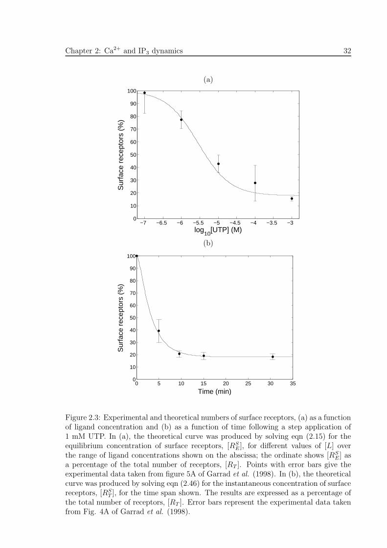
et al. (1998). Figure 2.3(a) shows the equilibrium number of surface receptors [RSE],
Chapter 2: Ca2+ and IP3 dynamics 31
computed using eqn (2.15), expressed as a percentage of [RT ], as a function of the
concentration of UTP. Also shown is the corresponding experimental data taken from
Fig. 5A of Garrad et al. (1998). The transient behaviour of the number of surface
receptors, following a 1 mM application of UTP at t = 0, is shown in Fig. 2.3(b),
where the solid line comes from the solution of eqn (2.46) and the points with error
bars are experimental values from Fig. 4A of Garrad et al. (1998).
Eqn (2.46) shows that the theoretical transient in Fig. 2.3(b) can be expressed as the
linear combination of the two solutions eλ1t and eλ2t, where the eigenvalues λ1 and λ2
are solutions of eqn (2.47). Figure 2.4 shows the variations in the real parts of these
two eigenvalues with respect to ligand concentration. The large relative difference in
magnitude between the eigenvalues is evident for ligand concentrations above about
1 µM. Here, the eigenvalues are real and so any solution is the sum of two decaying
exponential terms. The transient in [RST ] shown in Fig. 2.3(b) comprises two such
terms plus a constant term due to the immobile receptors, as seen from eqn (2.46).
The asymptotic values of the two curves labelled λ1 and λ2 in Fig. 2.4 are −0.0300
s−1 and −0.00622 s−1 which are in good agreement with the theoretical limiting values
of λ1 and λ2: λ1,∞ = −0.03 s−1 and λ2,∞ = −6.175 × 10⁻³ s−1. The approximations
for λ1 and λ2 given by eqns (2.48) and (2.49) are good also for [L]=1 mM. Because of
the large relative difference between the eigenvalues, for a sufficiently long time after
agonist application (≈ 2 minutes) the contribution of the eλ1t term can be ignored
and the transient in [RST ] shown in Fig. 2.3(b) can thus be approximated by a single
exponential term proportional to exp(−0.00618t). In the vicinity of 0.1 µM there is a
range of ligand concentrations for which the eigenvalues have imaginary parts, meaning
that [RST ] exhibits damped oscillatory behaviour; however, the imaginary parts turn
out to be too small for these oscillations to be readily observed over the time scale
used.
Figures 2.5(a)-(d) show the theoretical transients in IP3 concentration, Ca2+ concen-
tration, amount of PIP2 and amount of activated G-protein (Gα.GTP), respectively,
for a 1 mM application of UTP at t = 0. These transients were obtained from eqns
(2.13),(2.14) and (2.23)-(2.29), using initial conditions given by eqn (2.40). In Figs
2.5(a) -(c), solutions are plotted for three different values of the PIP2 replenishment
rate parameter : rr=10, 0.1 and 0.015 s−1. The smaller the value of rr the greater the
maximum depletion in the amount of PIP2 (Fig. 2.5(c)) and the faster the rate of decay
of the IP3 and Ca2+ concentrations (Fig. 2.5(a) and (b)). Lowering the value of rr
lowers the peak IP3 concentration and to a lesser extent the peak Ca2+ concentration.
The peak in activated G-protein (7.1%) is low due to the low ratio of ka to kd; also,
the amount of activated G-protein does not depend on rr.
Chapter 2: Ca2+ and IP3 dynamics 32
(a)
−7 −6.5 −6 −5.5 −5 −4.5 −4 −3.5 −30
10
20
30
40
50
60
70
80
90
100
log10
[UTP] (M)
Sur
face
rec
epto
rs (
%)
(b)
0 5 10 15 20 25 30 350
10
20
30
40
50
60
70
80
90
100
Time (min)
Sur
face
rec
epto
rs (
%)
Figure 2.3: Experimental and theoretical numbers of surface receptors, (a) as a functionof ligand concentration and (b) as a function of time following a step application of1 mM UTP. In (a), the theoretical curve was produced by solving eqn (2.15) for theequilibrium concentration of surface receptors, [RS
E], for different values of [L] overthe range of ligand concentrations shown on the abscissa; the ordinate shows [RS
E] asa percentage of the total number of receptors, [RT ]. Points with error bars give theexperimental data taken from figure 5A of Garrad et al. (1998). In (b), the theoreticalcurve was produced by solving eqn (2.46) for the instantaneous concentration of surfacereceptors, [RS
T ], for the time span shown. The results are expressed as a percentage ofthe total number of receptors, [RT ]. Error bars represent the experimental data takenfrom Fig. 4A of Garrad et al. (1998).
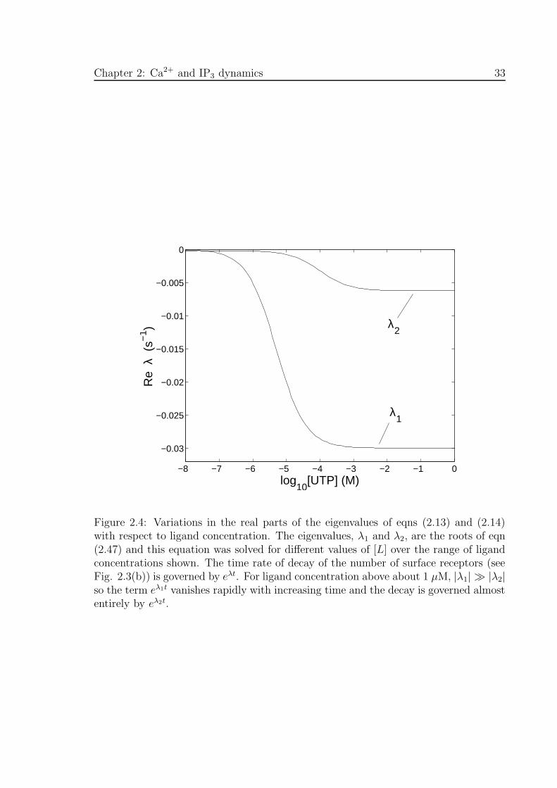
Chapter 2: Ca2+ and IP3 dynamics 33
−8 −7 −6 −5 −4 −3 −2 −1 0
−0.03
−0.025
−0.02
−0.015
−0.01
−0.005
0
log10
[UTP] (M)
Re
λ (
s−1 )
λ1
λ2
Figure 2.4: Variations in the real parts of the eigenvalues of eqns (2.13) and (2.14)with respect to ligand concentration. The eigenvalues, λ1 and λ2, are the roots of eqn(2.47) and this equation was solved for different values of [L] over the range of ligandconcentrations shown. The time rate of decay of the number of surface receptors (seeFig. 2.3(b)) is governed by eλt. For ligand concentration above about 1 µM, |λ1| � |λ2|so the term eλ1t vanishes rapidly with increasing time and the decay is governed almostentirely by eλ2t.
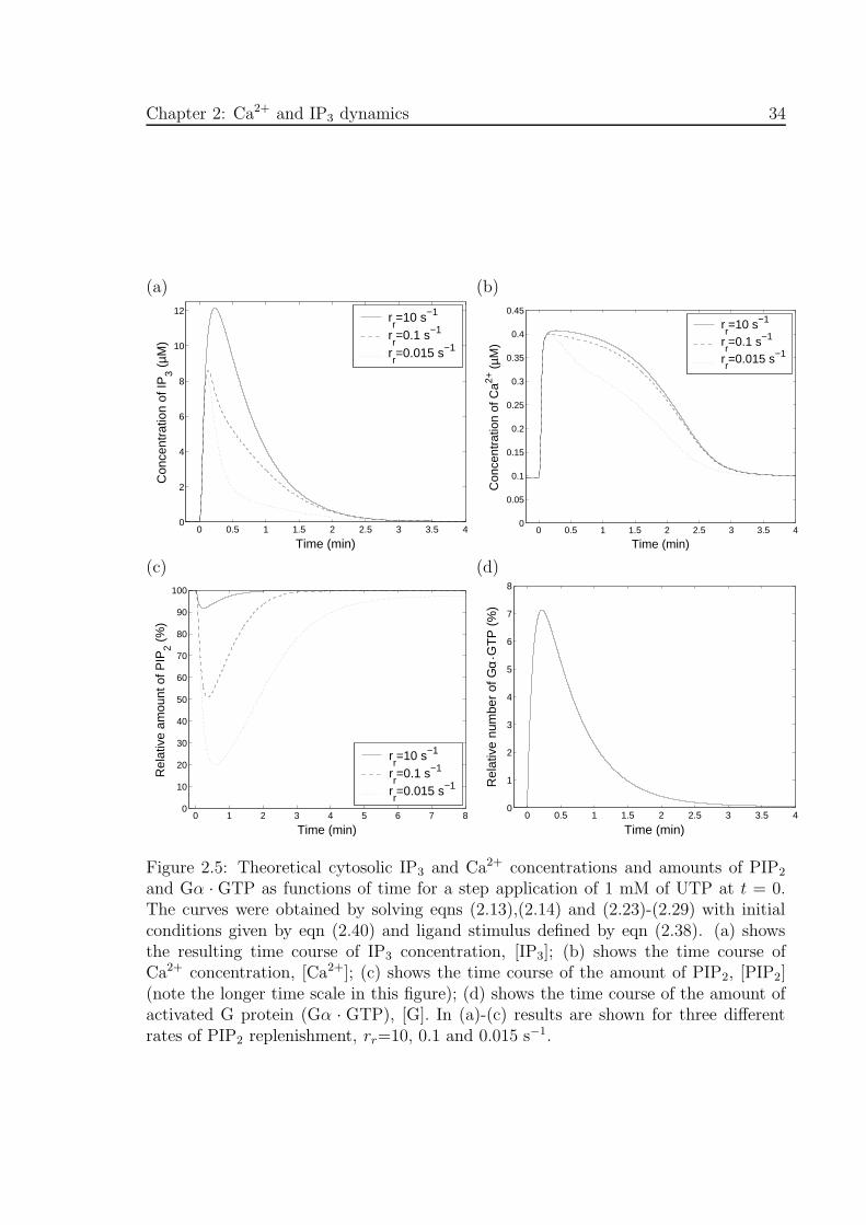
Chapter 2: Ca2+ and IP3 dynamics 34
(a) (b)
0 0.5 1 1.5 2 2.5 3 3.5 40
2
4
6
8
10
12
Time (min)
Con
cent
ratio
n of
IP3 (
µM)
rr=10 s−1
rr=0.1 s−1
rr=0.015 s−1
0 0.5 1 1.5 2 2.5 3 3.5 40
0.05
0.1
0.15
0.2
0.25
0.3
0.35
0.4
0.45
Time (min)
Con
cent
ratio
n of
Ca2+
(µM
)
rr=10 s−1
rr=0.1 s−1
rr=0.015 s−1
(c) (d)
0 1 2 3 4 5 6 7 80
10
20
30
40
50
60
70
80
90
100
Time (min)
Rel
ativ
e am
ount
of P
IP2 (
%)
rr=10 s−1
rr=0.1 s−1
rr=0.015 s−1
0 0.5 1 1.5 2 2.5 3 3.5 40
1
2
3
4
5
6
7
8
Time (min)
Rel
ativ
e nu
mbe
r of
Gα
GT
P (
%)
.
Figure 2.5: Theoretical cytosolic IP3 and Ca2+ concentrations and amounts of PIP2
and Gα · GTP as functions of time for a step application of 1 mM of UTP at t = 0.The curves were obtained by solving eqns (2.13),(2.14) and (2.23)-(2.29) with initialconditions given by eqn (2.40) and ligand stimulus defined by eqn (2.38). (a) showsthe resulting time course of IP3 concentration, [IP3]; (b) shows the time course ofCa2+ concentration, [Ca2+]; (c) shows the time course of the amount of PIP2, [PIP2](note the longer time scale in this figure); (d) shows the time course of the amount ofactivated G protein (Gα · GTP), [G]. In (a)-(c) results are shown for three differentrates of PIP2 replenishment, rr=10, 0.1 and 0.015 s−1.
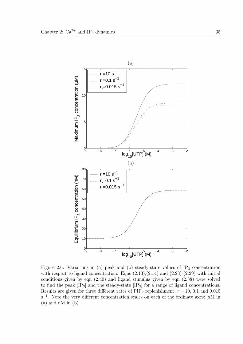
Chapter 2: Ca2+ and IP3 dynamics 35
(a)
−9 −8 −7 −6 −5 −4 −3 −20
5
10
15
log10
[UTP] (M)
Max
imum
IP3 c
once
ntra
tion
(µM
) rr=10 s−1
rr=0.1 s−1
rr=0.015 s−1
(b)
−9 −8 −7 −6 −5 −4 −3 −20
10
20
30
40
50
60
70
80
log10
[UTP] (M)
Equ
ilibr
ium
IP3 c
once
ntra
tion
(nM
) rr=10 s−1
rr=0.1 s−1
rr=0.015 s−1
Figure 2.6: Variations in (a) peak and (b) steady-state values of IP3 concentrationwith respect to ligand concentration. Eqns (2.13),(2.14) and (2.23)-(2.29) with initialconditions given by eqn (2.40) and ligand stimulus given by eqn (2.38) were solvedto find the peak [IP3] and the steady-state [IP3] for a range of ligand concentrations.Results are given for three different rates of PIP2 replenishment, rr=10, 0.1 and 0.015s−1. Note the very different concentration scales on each of the ordinate axes: µM in(a) and nM in (b).
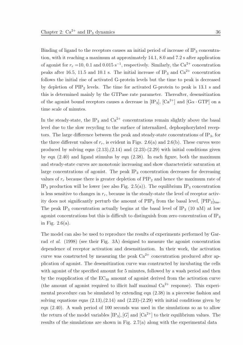
Chapter 2: Ca2+ and IP3 dynamics 36
Binding of ligand to the receptors causes an initial period of increase of IP3 concentra-
tion, with it reaching a maximum at approximately 14.1, 8.0 and 7.2 s after application
of agonist for rr =10, 0.1 and 0.015 s−1, respectively. Similarly, the Ca2+ concentration
peaks after 16.5, 11.5 and 10.1 s. The initial increase of IP3 and Ca2+ concentration
follows the initial rise of activated G-protein levels but the time to peak is decreased
by depletion of PIP2 levels. The time for activated G-protein to peak is 13.1 s and
this is determined mainly by the GTPase rate parameter. Thereafter, desensitization
of the agonist bound receptors causes a decrease in [IP3], [Ca2+] and [Gα · GTP] on a
time scale of minutes.
In the steady-state, the IP3 and Ca2+ concentrations remain slightly above the basal
level due to the slow recycling to the surface of internalized, dephosphorylated recep-
tors. The large difference between the peak and steady-state concentrations of IP3, for
the three different values of rr, is evident in Figs. 2.6(a) and 2.6(b). These curves were
produced by solving eqns (2.13),(2.14) and (2.23)-(2.29) with initial conditions given
by eqn (2.40) and ligand stimulus by eqn (2.38). In each figure, both the maximum
and steady-state curves are monotonic increasing and show characteristic saturation at
large concentrations of agonist. The peak IP3 concentration decreases for decreasing
values of rr because there is greater depletion of PIP2 and hence the maximum rate of
IP3 production will be lower (see also Fig. 2.5(a)). The equilibrium IP3 concentration
is less sensitive to changes in rr, because in the steady-state the level of receptor activ-
ity does not significantly perturb the amount of PIP2 from the basal level, [PIP2]bas.
The peak IP3 concentration actually begins at the basal level of IP3 (10 nM) at low
agonist concentrations but this is difficult to distinguish from zero concentration of IP3
in Fig. 2.6(a).
The model can also be used to reproduce the results of experiments performed by Gar-
rad et al. (1998) (see their Fig. 3A) designed to measure the agonist concentration
dependence of receptor activation and desensitization. In their work, the activation
curve was constructed by measuring the peak Ca2+ concentration produced after ap-
plication of agonist. The desensitization curve was constructed by incubating the cells
with agonist of the specified amount for 5 minutes, followed by a wash period and then
by the reapplication of the EC50 amount of agonist derived from the activation curve
(the amount of agonist required to illicit half maximal Ca2+ response). This experi-
mental procedure can be simulated by extending eqn (2.38) in a piecewise fashion and
solving equations eqns (2.13),(2.14) and (2.23)-(2.29) with initial conditions given by
eqn (2.40). A wash period of 100 seconds was used in the simulations so as to allow
the return of the model variables [IP3], [G] and [Ca2+] to their equilibrium values. The
results of the simulations are shown in Fig. 2.7(a) along with the experimental data
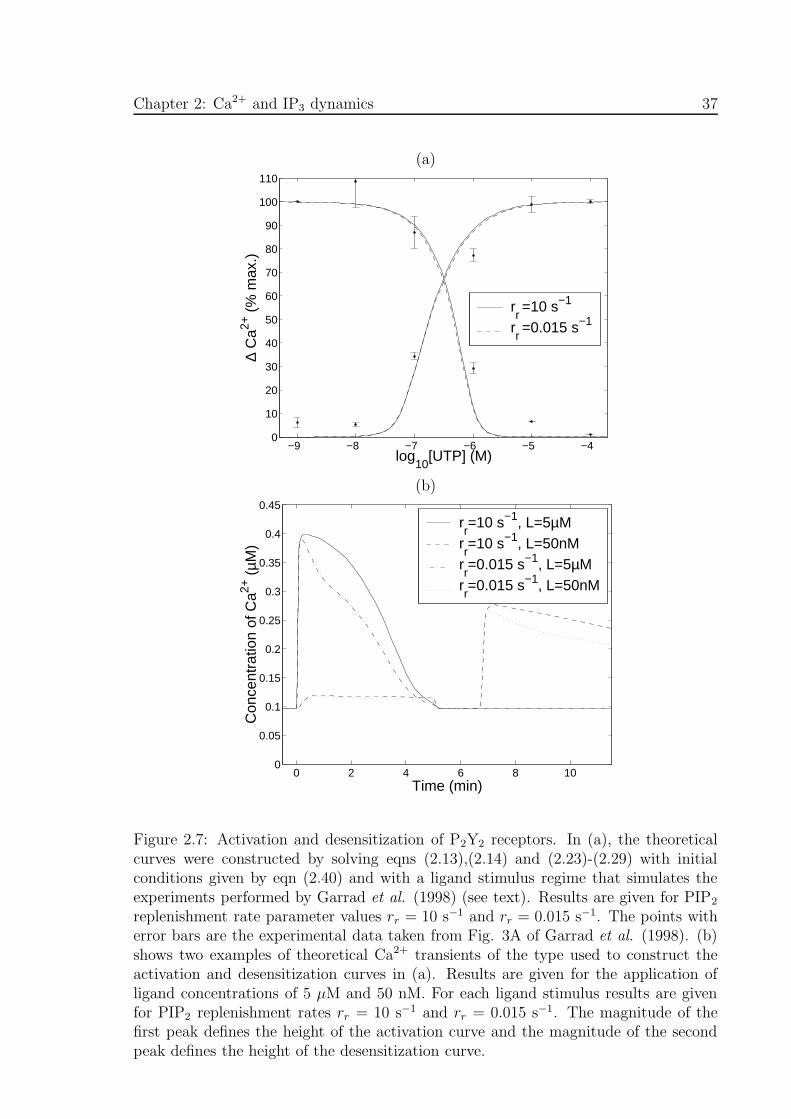
Chapter 2: Ca2+ and IP3 dynamics 37
(a)
−9 −8 −7 −6 −5 −40
10
20
30
40
50
60
70
80
90
100
110
log10
[UTP] (M)
∆ C
a2+ (
% m
ax.)
rr=10 s−1
rr=0.015 s−1
(b)
0 2 4 6 8 100
0.05
0.1
0.15
0.2
0.25
0.3
0.35
0.4
0.45
Time (min)
Con
cent
ratio
n of
Ca2+
(µM
)
rr=10 s−1, L=5µM
rr=10 s−1, L=50nM
rr=0.015 s−1, L=5µM
rr=0.015 s−1, L=50nM
Figure 2.7: Activation and desensitization of P2Y2 receptors. In (a), the theoreticalcurves were constructed by solving eqns (2.13),(2.14) and (2.23)-(2.29) with initialconditions given by eqn (2.40) and with a ligand stimulus regime that simulates theexperiments performed by Garrad et al. (1998) (see text). Results are given for PIP2
replenishment rate parameter values rr = 10 s−1 and rr = 0.015 s−1. The points witherror bars are the experimental data taken from Fig. 3A of Garrad et al. (1998). (b)shows two examples of theoretical Ca2+ transients of the type used to construct theactivation and desensitization curves in (a). Results are given for the application ofligand concentrations of 5 µM and 50 nM. For each ligand stimulus results are givenfor PIP2 replenishment rates rr = 10 s−1 and rr = 0.015 s−1. The magnitude of thefirst peak defines the height of the activation curve and the magnitude of the secondpeak defines the height of the desensitization curve.
Chapter 2: Ca2+ and IP3 dynamics 38
from Garrad et al. (1998), Fig. 3A. The shape of the desensitization curve is a
result of there being a low desensitization rate at low agonist concentrations, thus
leaving an abundance of unphosphorylated receptors when the agonist is re-applied.
At high agonist concentrations most of the receptors have been phosphorylated by
the time agonist is applied a second time, hence leading to a smaller response. The
activation and desensitization curves have been plotted for both rr = 10 s−1 and
rr = 0.015 s−1 (the curves for the case of rr = 0.1 s−1 have not been shown because
they do not markedly differ from those of the case rr = 10 s−1). The smaller the
value of rr, the greater the depletion of PIP2 from the membrane over the course of
the experiment and hence the smaller the Ca2+ response after the second application
of agonist. However, the desensitization curves for the two choices of rr are both
consistent with the experimental data. For rr = 10 s−1, the theoretically determined
EC50 and IC50 levels (the latter being the amount of agonist required to produce half
maximal desensitization) values were 180 nM and 489 nM respectively. For comparison,
the experimental values for EC50 and IC50 determined by Garrad et al. (1998) are 250
± 30 nM and 430 ± 100 nM (for the wild-type receptor).
Fig. 2.7(b) shows theoretical Ca2+ transients resulting from the simulated experimental
procedure used to construct the theoretical activation-desensitization curves in Fig.
2.7(a). Curves for an application of a small (50 nM) and a large (5 µM) concentration
of ligand are shown, for both values of rr. For each of the curves in Fig. 2.7(b),
the magnitude of the first peak corresponds to the height of the activation curve in
Fig. 2.7(a) and the magnitude of the second peak corresponds to the height of the
desensitization curve.
2.3.2 Parameter value selection
In this section, some explanation of how the unknown parameter values (indicated by
the ‘See text’ column in Table 2.1) were chosen. In some cases, recourse was made to
the parameter values determined in Chapter 3 where the model was used to fit other
experimental data for purinergic stimulation of cells.
In the absence of a definite value for K1 for the P2Y2 receptor, a value of 5 µM has
been used. This value was found to be optimal in fitting the model to experimental
data. Once K1 is set, the horizontal positioning of the theoretical curve in Fig. 2.3(a)
is determined by the value K2 (and to a less extent by the values of kr and ke, see
below) and this was chosen according to the experimental data in that figure.
The parameter ξ was adjusted to set the concentration of surface receptors at saturating
Chapter 2: Ca2+ and IP3 dynamics 39
agonist levels evident in the experimental data in Fig. 2.3(a). Without an immobile
fraction of receptors, the ratio kr/ke would have to be made larger to give a higher
rate of recycling of receptors. However, this however would mean a higher fraction of
dephosphorylated receptors at large agonist concentrations and would not allow a good
fit of the theoretical desensitization curve to the data in Fig. 2.7(a). Hence the ratio of
the values of kr and ke was kept small and adjusted to obtain a best fit in Fig. 2.3(a).
The value of ke itself was chosen to fit the decay rate of the experimental transient in
the number of surface receptors in Fig. 2.3(b).
The value for ka used was adapted from the results of Mahama and Linderman (1994)
for stochastic simulations of G-protein dynamics. In their paper, a simplified equation
is given where the rate of G-protein activation is proportional to the numbers of inactive
G-proteins and ligand bound receptors (see their eqn 6). The simplified theory is shown
to be applicable for the case of low diffusivity and no ligand switching, for which the
cell averaged encounter rate constant kc = 1 × 10⁻⁶ s−1 (see their Fig. 8). The value
for ka is assigned the value of this rate in the presence of the maximum number of
signalling receptors, hence ka = kcξ[RT ]. Estimates for the GTPase rate parameters
vary widely between cell types; for example, a range of 0.02 - 2 s−1 for the GTPase
rate, is quoted by Mahama and Linderman (1994). A suitable value for the G-protein
deactivation rate parameter, kd, determined in Chapter 3 from experimental rise time
data, lies in this range, and the same value was used in this chapter. Also determined
in Chapter 3 was the value of the dissociation constant for the binding of Ca2+ to PLC,
Kc = 0.4 µM, and this value was also used in this chapter.
The 1321N1 cells will be assumed to have a volume, ν = 5 × 10⁻¹⁶ m3. This value is
based on a spherically shaped cell of diameter approximately 10 µm.
The value of rr determines the rate of recovery of PIP2 levels after most of the P2Y2
receptors have been desensitized. The value of rr = 0.015 was chosen to allow recovery
of PIP2 in approximately 5 minutes, this being a similar recovery period to that mea-
sured by Varnai and Balla (1998) for angiotensin II stimulation of BAG cells (see their
Fig. 4B) and Waugh et al. (1999) for stimulation of the Chinese hamster ovary cells
expressing the human m1-muscarinic receptor (see their Fig. 3). For this value of rr,
the value of [(PIP2)T] was chosen so that a maximum of approximately 80% depletion
of PIP2 mass occurred during agonist stimulation, similar to that shown in Fig. 4B
of Varnai and Balla (1998). In practice, the levels and rate of PIP2 replenishment are
likely to vary widely between different cells. Hence the other two values of rr were
chosen to give a range of lower depletion levels of PIP2 during agonist stimulation.
The desired basal level of Ca2+ was to be approximately 100 nM (a typical value widely
Chapter 2: Ca2+ and IP3 dynamics 40
used in theoretical studies and the same as that used in Chapter 3). The desired
maximum possible change in Ca2+ concentration was chosen to be approximately 310
nM which lies within the experimentally determined range 282 ± 80 nM given in Garrad
et al. (1998). These concentrations were attained by making appropriate choices for
η1, η2, η3 and [(Ca2+)T], which are listed in Table 2.1. The numerically determined
values of [Ca2+]bas and hbas are 96.1 nM and 0.6158 which are close to the values of
[Ca2+]bas=115.6 nM and hbas=0.5737, computed using eqn (2.42).
Based on the observation by Luzzi et al. (1998) that in an unstimulated cell the con-
centration of IP3 is not more than a few tens of nano molar, the basal concentration
of IP3 has been chosen to be 10 nM. The three values of δ corresponding to the three
values of rr, chosen to obtain [IP3]bas = 10 nM, are given in Table 2.1. Also shown, for
the case of rr = 10 s−1, are the corresponding values of [G]bas, [PIP2]bas, [Ca2+]bas and
hbas. These values do not differ significantly from those of the cases rr = 0.1 s−1 and
0.015 s−1.
The value of kp was chosen, first roughly, so as to make the Ca2+ and IP3 transients
reach equilibrium levels, at saturating ligand concentrations, within approximately
five minutes. The values of α, kp and K1 all affect the horizontal positioning of the
theoretical activation and desensitization curves (and hence the EC50 values of these
curves). These parameters were adjusted to match the experimental data in Fig. 2.7(a).
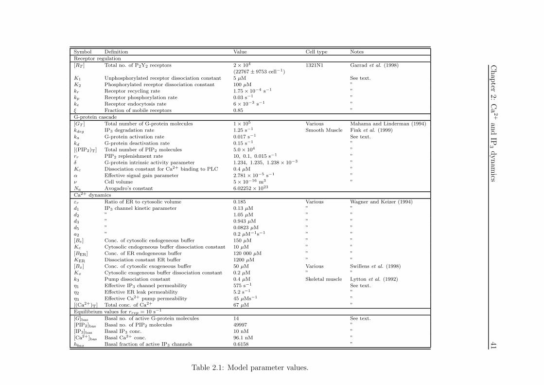
Chap
ter2:
Ca
2+
and
IP3
dynam
ics41
Symbol Definition Value Cell type Notes
Receptor regulation
[RT ] Total no. of P2Y2 receptors 2 × 10⁴ 1321N1 Garrad et al. (1998)(22767 ± 9753 cell−1)
K1 Unphosphorylated receptor dissociation constant 5 µM See text.K2 Phosphorylated receptor dissociation constant 100 µM ”kr Receptor recycling rate 1.75 × 10⁻⁴ s−1 ”kp Receptor phosphorylation rate 0.03 s−1 ”ke Receptor endocytosis rate 6 × 10⁻³ s−1 ”ξ Fraction of mobile receptors 0.85 ”
G-protein cascade
[GT ] Total number of G-protein molecules 1 × 10⁵ Various Mahama and Linderman (1994)kdeg IP3 degradation rate 1.25 s−1 Smooth Muscle Fink et al. (1999)
ka G-protein activation rate 0.017 s−1 See text.kd G-protein deactivation rate 0.15 s−1 ”[(PIP2)T] Total number of PIP2 molecules 5.0 × 10⁴ ”rr PIP2 replenishment rate 10, 0.1, 0.015 s−1 ”δ G-protein intrinsic activity parameter 1.234, 1.235, 1.238 × 10⁻³ ”Kc Dissociation constant for Ca2+ binding to PLC 0.4 µM ”α Effective signal gain parameter 2.781 × 10⁻⁵ s−1 ”ν Cell volume 5 × 10⁻¹⁶ m3 ”Na Avogadro’s constant 6.02252 × 10²³
Ca2+ dynamics
εr Ratio of ER to cytosolic volume 0.185 Various Wagner and Keizer (1994)d1 IP3 channel kinetic parameter 0.13 µM ” ”d2 ” 1.05 µM ” ”d3 ” 0.943 µM ” ”d5 ” 0.0823 µM ” ”a2 ” 0.2 µM−1s−1 ” ”[Be] Conc. of cytosolic endogeneous buffer 150 µM ” ”Ke Cytosolic endogeneous buffer dissociation constant 10 µM ” ”[BER] Conc. of ER endogeneous buffer 120 000 µM ” ”KER Dissociation constant ER buffer 1200 µM ” ”[Bx] Conc. of cytosolic exogeneous buffer 50 µM Various Swillens et al. (1998)Kx Cytosolic exogeneous buffer dissociation constant 0.2 µM ” ”k3 Pump dissociation constant 0.4 µM Skeletal muscle Lytton et al. (1992)η1 Effective IP3 channel permeability 575 s−1 See text.η2 Effective ER leak permeability 5.2 s−1 ”η3 Effective Ca2+ pump permeability 45 µMs−1 ”[(Ca2+)T] Total conc. of Ca2+ 67 µM ”
Equilibrium values for rrep = 10 s−1
[G]bas Basal no. of active G-protein molecules 14 See text.[PIP2]bas Basal no. of PIP2 molecules 49997 ”[IP3]bas Basal IP3 conc. 10 nM ”[Ca2+]bas Basal Ca2+ conc. 96.1 nM ”hbas Basal fraction of active IP3 channels 0.6158 ”
Table 2.1: Model parameter values.
Chapter 2: Ca2+ and IP3 dynamics 42
2.4 Discussion
Mathematical modelling has been carried out of the processes leading from agonist
stimulation of cells containing membrane metabotropic receptors, to the subsequent
Ca2+, IP3 and PIP2 response. A simplified and yet realistic model has been produced
that captures the essential elements of each part of the signal transduction process. A
quantitative account has successfully been given of the second messenger response of
single cells upon application of external ligand to metabotropic receptors.
The precise details of the mechanisms involved in metabotropic receptor activation and
desensitization depend on the receptor type (reviewed in Ferguson, 2001). For example,
the β2-adrenergic receptor (β2-AR) is phosphorylated by G-protein coupled receptor
kinases (GRKs) which preferentially bind to the agonist-bound receptor. Subsequent
binding of β-arrestins precludes interaction of the receptor with G-proteins hence caus-
ing desensitization. β-arrestin also acts as an endocytotic adaptor protein targeting
the β2-AR for internalization via clathrin coated pits. Other proteins such as the
Rab4 and Rab5 GTPases, both located in early endosomal membranes, are involved in
internalization, sorting and recycling of the β2-AR (Seachrist et al., 2000).
Less is known about the corresponding mechanisms for the P2Y2 receptor. This re-
ceptor has sites for phosphorylation by Protein Kinase C (PKC) and possible sites for
GRK phosphorylation (Garrad et al., 1998). Indeed, PKC has been shown to have
a role in P2Y2 receptor desensitization (Chen and Lin, 1999; Otero et al., 2000) but
phosphorylation by other protein kinases may be involved (Otero et al., 2000). In the
absence of definite information regarding the biochemical mechanisms for the regula-
tion of the P2Y2 receptor, the mechanisms given above for the β2-AR have been used
to construct the mathematical model. This is justified by the fact that the regulation
of the P2Y2 receptor involves the same processes given above.
The effects of internalization of ligand (for example, ligand dependent sorting in endo-
somes) have been neglected, as have also receptor degradation and insertion at the cell
surface, since these processes generally become significant only after hours of continual
application of agonist whereas the present model is only concerned with times of not
more than several tens of minutes.
Recent studies suggest the importance of the spatial localization of membrane and
cytosolic components of second messenger signalling (Golovina and Blaustein, 1997;
Haugh et al., 1998). The model presented here, while neglecting this consideration,
was found to be adequate in describing the experimental data. It is straight forward
however to generalize the model to include diffusion of subspecies, but this is beyond

Chapter 2: Ca2+ and IP3 dynamics 43
the scope of the present work.
The processes linking active metabotropic receptors to production of IP3 may comprise
more than one pathway depending on the cell type. Each pathway may comprise
different subtypes of G-protein subunits and PLC. In smooth muscle the P2Y2 receptor
activates both PLC-β1 via Gαq/11 and PLC-β3 via Gβγi3 (Murthy and Makhlouf,
1998). In Chinese hamster ovary cells, however, P2Y2 functionally couples only to
PLC-β3 (Strassheim and Williams, 2000). In the model presented here it is assumed
that there is only one pathway with one type of G-protein (Gαq/11) and PLC (PLC-β1).
All types of phospholipase C (PLC-β, PLC-γ, PLC-δ) require the presence of Ca2+ for
activation (Rebbecchi and Pentyala, 2000) . Strong activation of PIP2 hydrolysis by
Ca2+ is evident in many cell systems (Harootunian et al., 1991; Taylor et al., 1991;
Capozzi et al., 1999) but there is evidence that this is only true when PLC-δ is involved
(Allen et al., 1997). This activation is also evident in the results of Hirose et al. (1999),
to which the present model will also be applied in Chapter 3, and so Ca2+ activation
of PLC is included in the model. However, the model G-protein cascade involves only
PLC-β and so the catalytic effect of Ca2+ on PIP2 hydrolysis is assumed to be due to
activation of PLC-β by Ca2+.
Degradation of IP3 may involve a 3-kinase (Takazawa et al., 1990) or a 5-phosphatase
(Verjans et al., 1994). The 3-kinase has shown to be stimulated by Ca2+ resulting
in a Ca2+ dependent IP3 degradation rate. For the purposes of this study, however,
it is assumed that IP3 is metabolized by the Ca2+ independent 5-phosphatase which
justifies using a constant value for kdeg.
While ryanodine channels play a vital role in cardiac Ca2+ dynamics (see Section 3 of
Chapter 1), their role in metabotropic receptor pathways is less clear. Some studies
have identified interactions between the two channel types in cells (Haak et al., 2001).
However, the low ratio of ryanodine to IP3 channel density found in many cells (for
example ≈ 0.1 in intestinal smooth muscle (Wibo and Godfraind, 1994)) together
with the micromolar Ca2+ concentration required to initiate CICR means that the
contribution of CICR to global is often far smaller than that due to IICR. For this
reason, the inclusion of CICR due to the ryanodine channel has not been included in
the modelling.
A simplified yet realistic model has been chosen for the IP3 channel, a model that
has the potential to allow Ca2+ oscillations and waves (see for example De Young and
Keizer, 1992; Wagner and Keizer, 1994). The parameter values chosen here were such
that no oscillations occur for any concentration of IP3, this being consistent with the

Chapter 2: Ca2+ and IP3 dynamics 44
experimental evidence. Simulations show that both sustained and damped Ca2+ oscil-
lations are ubiquitous when the lower value for the Ca2+ pump dissociation constant,
k3 = 0.1µM representing the SERCA2 isoform, is used. That the higher value used
here, k3 = 0.4µM corresponding to the SERCA1 isoform, supresses the occurrence of
oscillations may indicate this is the dominant isoform in these cells.
Many of the rate parameter values for the chemical reactions in the detailed signal
transduction model are unknown. It has been the approach here to use, without
evidence to the contrary, the assumptions of rapid kinetics and subsaturation binding
to simplify the equations for the reactions (see Appendix A). These assumptions do not
affect the qualitative behaviour of the system as a whole but do allow each submodule in
the model to be characterized by a minimal number of free parameters. This can allow
unambiguous determination of parameter values for fitting the model to experimental
data.
The relative difference in magnitudes between the desensitization rate parameter kp
and the receptor endocytosis and recycling parameters, ke and kr respectively, has en-
sured that desensitization occurs over a faster time scale than internalization. As seen
in Fig. 2.5(b), for a step application of 1 mM UTP, the theoretical IP3 concentration
transient has a decay half time of approximately 30 seconds whereas, as shown in Fig.
2.3(a), the decay in the number of surface receptors has a half time of approximately
2.5 minutes. That desensitization occurs more rapidly than internalization appears
to be typical of the P2Y2 receptor, although the absolute rates may vary between
preparations. For example, in another experiment of the stimulation of 1321N1 cells
with UTP (Sromek and Harden, 1998) maximal accumulation of inositol phosphates
occurred with a half time of approximately 2.5 minutes, whereas the half time of the
decay of surface receptors was approximately 15 minutes. The faster rate of desensi-
tization relative to internalization is typical of other types of metabotropic receptors;
for a review see Ferguson (2001) and Bunemann et al. (1999).
In Figs. 2.6(a) and 2.6(b) both the maximum and steady-state IP3 concentration curves
are monotonic increasing and plateau at large concentrations of agonist due to receptor
saturation. For raised levels of Ca2+ and IP3 to be maintained over extended periods,
recycling of dephosphorylated receptors and resupply of membrane PIP2 are essential.
Typically in experiments cells are treated with LiCl and measurements of total inositol
phosphate (including species of phosphorylated IP3) accumulation is measured after
some fixed time. Treatment with LiCl alters the pathway of resupply of PIP2 to the
membrane and for this reason such data is not directly applicable to this model. There
is however some data available of measurements of equilibrium IP3 concentration with
Chapter 2: Ca2+ and IP3 dynamics 45
respect to ligand (Waugh et al. 1999) which confirms the qualitative form of the curves
in Fig. 2.6(b).
The theoretical time taken for IP3 concentration to peak after application of agonist
is in agreement with the 5-20 second range observed by Strøbæk et al. (1996) for
purinergic stimulation of human coronary smooth muscle cells. Experimental studies
suggest that the range of concentrations of IP3 attainable in cells is from tens of nM
to tens of µM (Horstman et al., 1988; Khodakhah et al., 1993; Luzzi et al., 1998). The
modelling in this chapter has predicted a concentration range for IP3 of 10 nM (basal)
to approximately 12 µM at saturating levels of agonist.
An important result of this study comes from the modelling of mechanisms for PIP2
depletion and resupply. Using reasonable estimates for the replenishment rate param-
eter, rr, and level of total PIP2, [(PIP2)T], the results show that the level of PIP2
depletion has a significant effect on the Ca2+ and IP3 response. For the lowest rate of
PIP2 resupply, rr = 0.015 s−1, the IP3 and Ca2+ concentrations were decreased by up
to 80% and 30% respectively, compared to the concentrations at the highest rate of
resupply, rr = 10 s−1 (see Fig 2.5(a),(b)). Depletion of PIP2 may therefore contribute
significantly to the deactivation of the signal transduction processes in cells.
Estimates of the density of PIP2 molecules in the plasma membrane are not widely
available from the literature. However, using the method explained above to determine
a likely value for [(PIP2)T], the number of PIP2 molecules turns out to be comparable
to the number of receptors and G protein molecules, [RT ] and [GT ] respectively.
The mathematical model developed in this chapter could be extended to include the
extra features discussed in Chapter 1. In the case of multiple signalling pathways
the equations need to be augmented to include the additional species involved. A
possible complication is that species of the same type will compete for binding sites
on the same target molecules, however the method described in Appendix D (used
in the modelling in Chapter 3) could be used to simplify these effects. To model
heterogeneous distributions of signalling molecules in the cell membrane or cytosol, it
may be necessary to include diffusion of these molecules in the model. The extended
model will be in the form of a boundary value problem with the inclusion of Laplacian
terms to describe the diffusion of species, that is, a set of coupled reaction-diffusion
equations. Indeed, the model for the Ca2+ dynamics, described in Section 2.3 of this
chapter has been previously extended by others to include diffusion of Ca2+ and exhibits
travelling Ca2+ wave front solutions (Jafri and Keizer, 1995). The topic of intracellular
diffusion will be returned to in Chapter 3, where the diffusion of the green fluorescent
protein-pleckstrin homology domain (GFP-PHD) molecule in the cytosol is studied,
Chapter 2: Ca2+ and IP3 dynamics 46
and also in Chapter 4 which concerns intracellular Ca2+ waves, where diffusion of Ca2+
plays an important role.
A more complete mathematical model for a single cell could be build from the model
devised in this chapter by adding the requisite components. In some applications it
may be necessary to add additional intracellular Ca2+ stores such such as mitochondria
or peripheral SR/ER. This is currently being carried out by the author to model the
Ca2+ dynamics in A7r5 rat aortal smooth muscle cells. The microstructure of these
cells, which exhibits separate central and peripheral SR compartments, has significant
implications for the Ca2+ dynamics in these cells. In other applications, modelling of
the target processes of intracellular Ca2+ release may be required such as the Ca2+
regulated contraction in myocytes which begins with the binding of Ca2+ to troponin
C in skeletal muscle or to calmodulin in smooth muscle (Somlyo and Somlyo, 1994).
Also, the single cell model could be used to build models of multicellular systems. Such
a model would comprise a set of equations for each cell, with extra terms describing
the chemical, electrical or mechanical coupling between adjacent cells, for example
leak terms to model the diffusion of IP3 through gap junctions. A multicellular model
devised in this way could be used to study agonist induced behaviour of tissue such as
contraction of blood vessels or intercellular Ca2+ waves in astrocytes (Scemes, 2000).
47
Chapter 3
Modelling the dynamics of thegreen fluorescent protein-pleckstrinhomology domain construct
Recent observations have been made regarding the generation of inositol 1,4,5 - trispho-
sphate (IP3), using chimeras of green fluorescent protein and the pleckstrin homology
domain of phospholipase C-δ. In this chapter a model is presented giving the quan-
titative relations between the green fluorescent protein-pleckstrin homology domain
(GFP-PHD) construct and membrane phosphatidylinositol 4,5-bisphosphate (PIP2)
levels as well as the concentration of IP3, the product of hydrolysis of PIP2. The model
can correctly reproduce the dependence of cytosolic GFP-PHD fluorescence on IP3
concentration. This model extends the one in Chapter 2 dealing with the processes
governing the production of IP3 and the subsequent calcium (Ca2+) changes in cells
following activation of metabotropic receptors. This model is applied to the case of
purinergic P2Y2 receptor activation in Madin-Darby canine kidney (MDCK) epithelial
cells with adenosine triphosphate (ATP) (Hirose et al., 1999). It is shown that it can
correctly reproduce the dependence of GFP-PHD fluorescence on the concentration
of P2Y2 receptor ligand, as well as the temporal changes of GFP-PHD fluorescence
following application of ligand.
3.1 Introduction
Calcium ions (Ca2+) are an important signalling agent for many aspects of cellular
activity (Berridge, 1997; 1998). These ions can enter cells through either voltage-gated
or receptor-activated channels in the plasmalemma, or they can be released from stores
inside the cell. A principal store is the endoplasmic reticulum and here release can occur
Chapter 3: Dynamics of the GFP-PHD 48
through the action of Ca2+ on ryanodine receptors or through the combined action of
Ca2+ and inositol 1,4,5-trisphosphate (IP3) on IP3 receptors. It is also apparent that
IP3 plays an important role in intercellular communication through its ability to diffuse
through the gap junctions connecting cells and thus initiate Ca2+ release from internal
stores in neighbouring cells (Kostyuk and Verkhratsky, 1995; Berridge, 1993; 1998).
Much information about the action of Ca2+ has been obtained from experiments in
which it is bound to a fluorescent marker and the subsequent spatial and temporal
behaviour observed using confocal microscopy. Considerably less is known about the
behaviour of IP3, since it does not bind to fluorescent markers and thus cannot be
directly observed. However, recently a method has been developed for obtaining in-
formation via an indirect imaging technique. This method depends crucially on the
interaction between IP3, phosphatidylinositol 4,5-bisphosphate (PIP2) and a molecule
that can be tagged with a fluorescent marker. The latter is the pleckstrin homology
domain (PHD) of phospholipase C (PLC) which binds to green fluorescent protein
(GFP) to form the complex GFP-PHD. In the absence of IP3, GFP-PHD binds to
PIP2 which remains fixed in the membrane of the cell and thus the fluorescence is
concentrated there. However, GFP-PHD binds to IP3 with a much higher affinity than
to PIP2 (Lemmon et al., 1995; Ferguson et al., 1995); furthermore, the bound complex
of IP3 with GFP-PHD is mobile and can diffuse into the cytosol, causing an increase of
fluorescence there and a corresponding decrease in the membrane (Stauffer et al., 1998;
Varnai and Balla, 1998; Hirose et al., 1999; Nash et al., 2001). The overall conclusion
is that the spatial and temporal behaviour of IP3 is reflected in the dynamics of the
PHD and this can be observed because of the GFP tagging.
This chapter presents a mathematical model for the process of translocation of GFP-
PHD to and from the membrane in the presence of IP3. The model is formulated
as a boundary value problem, taking into account the interactions of IP3 both in the
membrane and in the cytosol and the transport between the two regions. A number of
simplifications are made, leading to equations relating fluorescence change to IP3 and
membrane PIP2 concentrations.
The experimental results of Hirose et al. (1999) are for Madin-Darby canine kidney
(MDCK) epithelial cells stimulated with adenosine triphosphate (ATP). The ATP acts
on P2Y2 receptors and initiates a G-protein cascade leading to the production of IP3.
The processes of P2Y2 receptor activation, desensitization and sequestration play an
important role in determining the time course of IP3 concentration. These processes
have been modelled in Chapter 2 and this theory will be used in conjunction with the
new theory presented here to give a unified account of the steps leading from receptor
Chapter 3: Dynamics of the GFP-PHD 49
activation to translocation of GFP-PHD.
3.2 Methods
3.2.1 Spatial and temporal dynamics of the pleckstrin homol-ogy domain - green fluorescent protein construct
A schematic diagram of the mechanisms involved in the GFP-PHD dynamics is shown
in Fig. 3.1. Part A of the diagram shows how IP3 competes with PIP2 for the binding
site on the GFP-PHD molecule. Part B shows that both the unbound GFP-PHD
and that bound with IP3 may dissociate and reassociate with the membrane. Also
GFP-PHD may interact with IP3 inside the cytosol.
First, the full set of equations governing the concentrations of subspecies of GFP-PHD
in the membrane and cytosol is presented. In the first instance, it is assumed that GFP-
PHD does not compete with PLC for binding with PIP2 and that the amount of PIP2
in the membrane is constant. Next, the equations are simplified using the assumptions
of rapid kinetics and of sub-saturation binding. The boundary value problem for the
cytosolic concentration of GFP-PHD is derived and a conservation condition relating
the concentrations of subspecies of GFP-PHD given. Next, the assumption is made
that the concentrations of GFP-PHD, PIP2 and IP3 are uniform across the membrane.
The conservation condition is then used to derive an expression for the relative cytosolic
fluorescence change as a function of IP3 concentration, at equilibrium. The parameters
in this equilibrium equation can be determined experimentally. An expression for the
ratio of membrane and cytosolic concentrations of GFP-PHD expressed in terms of
these parameters and valid for the fully time-dependent case is then derived and the
modifications to the theory in the case of depletion of PIP2 discussed. Finally, the
mathematical relation between cytosolic fluorescence and concentration of GFP-PHD
is described.
In Appendix D, the theory is extended to include competition of GFP-PHD with PLC
for binding with PIP2; such competition may modify the GFP-PHD dynamics as well
as the rate of hydrolysis of PIP2 by PLC. It is demonstrated how this extended theory
can be simplified so that competitive effects can be ignored.
At the end of this Methods section there is a summary that collects together the main
equations that are used in the calculations reported in this chapter.
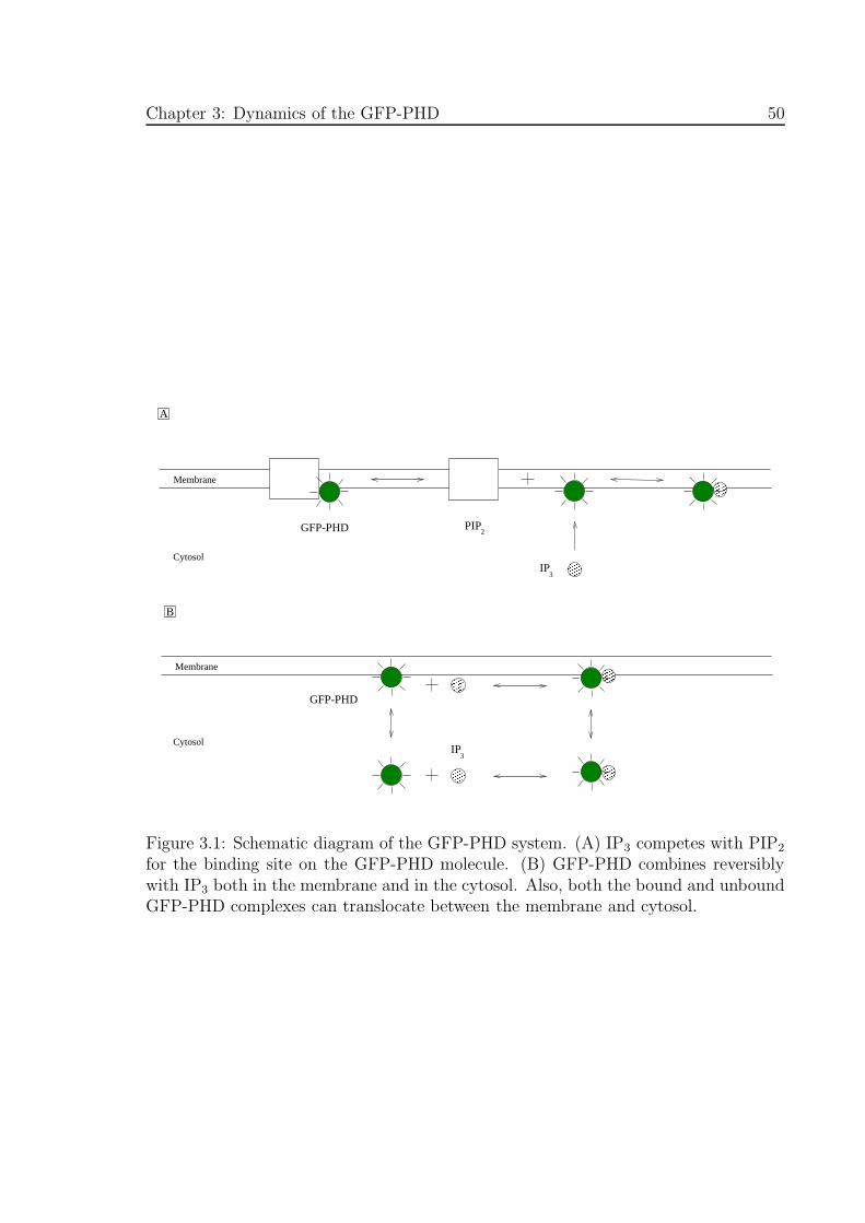
Chapter 3: Dynamics of the GFP-PHD 50
IP3
IP3
���������
���������
GFP-PHD
���������
���������
���������������
���������
���������������
���������������
������
������
���������������
���������������
2
Membrane
PIP
Membrane
GFP-PHD
B
A
Cytosol
Cytosol
Figure 3.1: Schematic diagram of the GFP-PHD system. (A) IP3 competes with PIP2
for the binding site on the GFP-PHD molecule. (B) GFP-PHD combines reversiblywith IP3 both in the membrane and in the cytosol. Also, both the bound and unboundGFP-PHD complexes can translocate between the membrane and cytosol.

Chapter 3: Dynamics of the GFP-PHD 51
3.2.2 Mathematical model of the GFP-PHD dynamics
Consider a cell of arbitrary shape comprising an intracellular space B bounded by a
closed membrane ∂B. An arbitrary point x will be written as v (“volume”) when
it lies wholly within the cytosol and s (“surface”) when it lies on the cell membrane.
The GFP-PHD fusion construct is a protein molecule that is completely free to diffuse
through the cytoplasm of the cell (assumed to be unhindered by intracellular organelles
and membranes) but interacts with the cell membrane in a special way (see Fig. 3.2,
where ‘GFP-PHD’ has been abbreviated as ‘GP’). Each GFP-PHD molecule may bind
a single molecule of IP3. Let the cytosolic concentrations of GFP-PHD, unbound and
bound to IP3 be [GP] and [GP · IP3] respectively, these being functions of v and t and
let the surface concentrations of membrane bound GFP-PHD, unbound and bound to
IP3, be [GPM] and [GP · IP3M] respectively, these being functions of s and t. Also
residing in the cell membrane is PIP2 which binds with GFP-PHD thereby ‘tethering’
it to the membrane; that is, after the GFP-PHD molecule is bound to PIP2 it cannot
diffuse directly back into the cytosol. Let the surface concentrations of PIP2 unbound
and bound to GFP-PHD, be [PIP2M] and [GP·PIP2
M] respectively, these also being
functions of s and t.
Using a continuum approach to diffusion, a set of adsorption-reaction-diffusion partial
differential equations can be formulated that govern the space-time concentrations
of the above substances. In the following, the concentration of IP3 is treated as a
given function of space and time; thus [IP3] ≡ [IP3](x, t). The concentrations of the
substances [GP](v, t) and [GP ·IP3](v, t) in the cytosol satisfy the differential equations
∂[GP]
∂t= DGP∇2[GP] − k+
1 [IP3][GP] + k−1 [GP · IP3], (3.1)
∂[GP · IP3]
∂t= DGP∇2[GP · IP3] − k−1 [GP · IP3] + k+
1 [IP3][GP], (3.2)
where DGP is the bulk diffusion coefficient of GFP-PHD in the cytosol, assumed to be
the same whether bound or unbound to IP3 and k+1 , k−1 are the forward and reverse
rate constants for the binding of IP3 to GFP-PHD.
The important chemical reactions occurring at each point of the membrane are de-
picted in Fig. 3.2. The species [GP] = [GP](s, t) and [GP · IP3] = [GP · IP3](s, t)
take on their concentrations at the membrane in these reactions; in addition to these
membrane kinetics, species [GP] and [GP · IP3] can diffuse throughout the cytosol. In
the model presented here, GFP-PHD is allowed to actively associate and dissociate
non-specifically with the membrane (without the need for the presence of adsorption
sites) but once within the membrane IP3 competes with PIP2 for the binding site on
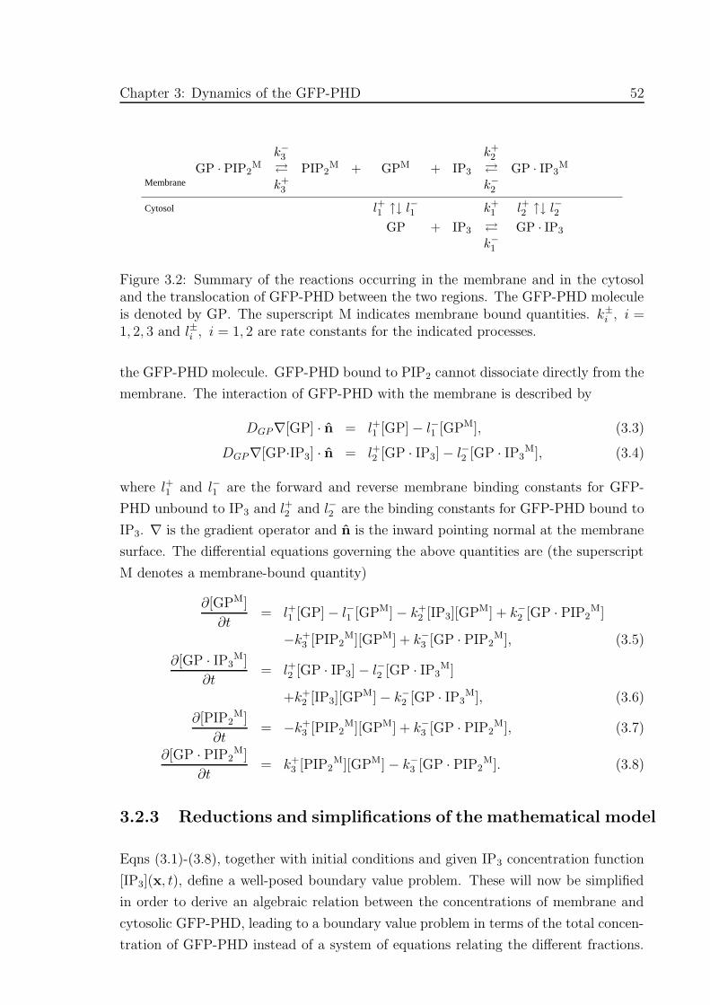
Chapter 3: Dynamics of the GFP-PHD 52
Membrane
Cytosol
k−3 k
+2
GP · PIP2M
� PIP2M + GPM + IP3 � GP · IP3
M
k+3 k
−2
l+1 ↑↓ l
−1 k
+1 l
+2 ↑↓ l
−2
GP + IP3 � GP · IP3
k−1
Figure 3.2: Summary of the reactions occurring in the membrane and in the cytosoland the translocation of GFP-PHD between the two regions. The GFP-PHD moleculeis denoted by GP. The superscript M indicates membrane bound quantities. k±i , i =1, 2, 3 and l±i , i = 1, 2 are rate constants for the indicated processes.
the GFP-PHD molecule. GFP-PHD bound to PIP2 cannot dissociate directly from the
membrane. The interaction of GFP-PHD with the membrane is described by
DGP∇[GP] · n = l+1 [GP] − l−1 [GPM], (3.3)
DGP∇[GP·IP3] · n = l+2 [GP · IP3] − l−2 [GP · IP3M], (3.4)
where l+1 and l−1 are the forward and reverse membrane binding constants for GFP-
PHD unbound to IP3 and l+2 and l−2 are the binding constants for GFP-PHD bound to
IP3. ∇ is the gradient operator and n is the inward pointing normal at the membrane
surface. The differential equations governing the above quantities are (the superscript
M denotes a membrane-bound quantity)
∂[GPM]
∂t= l+1 [GP] − l−1 [GPM] − k+
2 [IP3][GPM] + k−2 [GP · PIP2M]
−k+3 [PIP2
M][GPM] + k−3 [GP · PIP2M], (3.5)
∂[GP · IP3M]
∂t= l+2 [GP · IP3] − l−2 [GP · IP3
M]
+k+2 [IP3][GPM] − k−2 [GP · IP3
M], (3.6)
∂[PIP2M]
∂t= −k+
3 [PIP2M][GPM] + k−3 [GP · PIP2
M], (3.7)
∂[GP · PIP2M]
∂t= k+
3 [PIP2M][GPM] − k−3 [GP · PIP2
M]. (3.8)
3.2.3 Reductions and simplifications of the mathematical model
Eqns (3.1)-(3.8), together with initial conditions and given IP3 concentration function
[IP3](x, t), define a well-posed boundary value problem. These will now be simplified
in order to derive an algebraic relation between the concentrations of membrane and
cytosolic GFP-PHD, leading to a boundary value problem in terms of the total concen-
tration of GFP-PHD instead of a system of equations relating the different fractions.
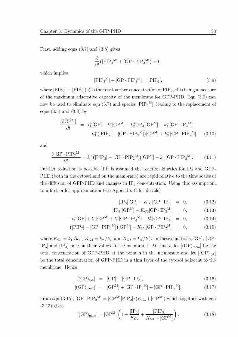
Chapter 3: Dynamics of the GFP-PHD 53
First, adding eqns (3.7) and (3.8) gives
∂
∂t([PIP2
M] + [GP · PIP2M]) = 0,
which implies
[PIP2M] + [GP · PIP2
M] = [PIP2], (3.9)
where [PIP2] ≡ [PIP2](s) is the total surface concentration of PIP2, this being a measure
of the maximum adsorptive capacity of the membrane for GFP-PHD. Eqn (3.9) can
now be used to eliminate eqn (3.7) and species [PIP2M], leading to the replacement of
eqns (3.5) and (3.8) by
∂[GPM]
∂t= l+1 [GP] − l−1 [GPM] − k+
2 [IP3][GPM] + k−2 [GP · IP3M]
−k+3 ([PIP2] − [GP · PIP2
M])[GPM] + k−3 [GP · PIP2M] (3.10)
and
∂[GP · PIP2M]
∂t= k+
3 ([PIP2] − [GP · PIP2M])[GPM] − k−3 [GP · PIP2
M]. (3.11)
Further reduction is possible if it is assumed the reaction kinetics for IP3 and GFP-
PHD (both in the cytosol and on the membrane) are rapid relative to the time scales of
the diffusion of GFP-PHD and changes in IP3 concentration. Using this assumption,
to a first order approximation (see Appendix C for details)
[IP3][GP] −KG1[GP · IP3] = 0, (3.12)
[IP3][GPM] −KG2[GP · IP3M] = 0, (3.13)
−l+1 [GP] + l−1 [GPM] + l−2 [GP · IP3M] − l+2 [GP · IP3] = 0, (3.14)
([PIP2] − [GP · PIP2M])[GPM] −KG3[GP · PIP2
M] = 0, (3.15)
where KG1 = k−1 /k+1 , KG2 = k−2 /k
+2 and KG3 = k−3 /k
+3 . In these equations, [GP], [GP·
IP3] and [IP3] take on their values at the membrane. At time t, let [(GP)mem] be the
total concentration of GFP-PHD at the point s in the membrane and let [(GP)cyt]
be the total concentration of GFP-PHD in a thin layer of the cytosol adjacent to the
membrane. Hence
[(GP)cyt] = [GP] + [GP · IP3], (3.16)
[(GP)mem] = [GPM] + [GP · IP3M] + [GP · PIP2
M]. (3.17)
From eqn (3.15), [GP · PIP2M] = [GPM][PIP2]/(KG3 +[GPM]) which together with eqn
(3.13) gives
[(GP)mem] = [GPM]
(1 +
[IP3]
KG2+
[PIP2]
KG3 + [GPM]
). (3.18)
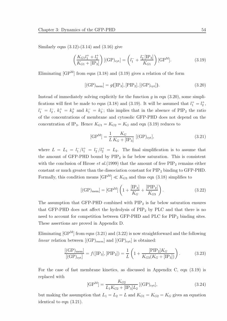
Chapter 3: Dynamics of the GFP-PHD 54
Similarly eqns (3.12)-(3.14) and (3.16) give
(KG1l
+1 + l+2
KG1 + [IP3]
)[(GP)cyt] =
(l−1 +
l−2 [IP3]
KG1
)[GPM]. (3.19)
Eliminating [GPM] from eqns (3.18) and (3.19) gives a relation of the form
[(GP)mem] = g([IP3], [PIP2], [(GP)cyt]). (3.20)
Instead of immediately solving explicitly for the function g in eqn (3.20), some simpli-
fications will first be made to eqns (3.18) and (3.19). It will be assumed that l+1 = l+2 ,
l−1 = l−2 , k+1 = k+
2 and k−1 = k−2 ; this implies that in the absence of PIP2 the ratio
of the concentrations of membrane and cytosolic GFP-PHD does not depend on the
concentration of IP3. Hence KG1 = KG2 = KG and eqn (3.19) reduces to
[GPM] =1
L
KG
KG + [IP3][(GP)cyt], (3.21)
where L = L1 = l−1 /l+1 = l−2 /l
+2 = L2. The final simplification is to assume that
the amount of GFP-PHD bound by PIP2 is far below saturation. This is consistent
with the conclusion of Hirose et al.(1999) that the amount of free PIP2 remains either
constant or much greater than the dissociation constant for PIP2 binding to GFP-PHD.
Formally, this condition means [GPM] � KG3 and thus eqn (3.18) simplifies to
[(GP)mem] = [GPM]
(1 +
[IP3]
KG+
[PIP2]
KG3
). (3.22)
The assumption that GFP-PHD combined with PIP2 is far below saturation ensures
that GFP-PHD does not affect the hydrolysis of PIP2 by PLC and that there is no
need to account for competition between GFP-PHD and PLC for PIP2 binding sites.
These assertions are proved in Appendix D.
Eliminating [GPM] from eqns (3.21) and (3.22) is now straightforward and the following
linear relation between [(GP)mem] and [(GP)cyt] is obtained:
[(GP)mem]
[(GP)cyt]= f([IP3], [PIP2]) =
1
L
(1 +
[PIP2]KG
KG3(KG + [IP3])
). (3.23)
For the case of fast membrane kinetics, as discussed in Appendix C, eqn (3.19) is
replaced with
[GPM] =KG2
L1KG2 + [IP3]L2[(GP)cyt], (3.24)
but making the assumption that L1 = L2 = L and KG1 = KG2 = KG gives an equation
identical to eqn (3.21).

Chapter 3: Dynamics of the GFP-PHD 55
3.2.4 The simplified equations of the GFP-PHD dynamics
Using eqns (3.1)-(3.8), it can be shown that
∂
∂t([GP] + [GP · IP3]) = DGP∇2([GP] + [GP · IP3]), x ∈ B, (3.25)
DGP∇([GP] + [GP · IP3]) · n =∂
∂t([GPM] + [GP · IP3
M]
+ [GP · PIP2M]), x ∈ ∂B, (3.26)
and using the definitions of eqns (3.16), (3.17) and (3.20) the reduced problem governing
the adsorption-diffusion of GFP-PHD is given by
∂[(GP)cyt]
∂t= DGP∇2[(GP)cyt], x ∈ B, (3.27)
DGP∇[(GP)cyt] · n =∂
∂tg([IP3], [PIP2], [(GP)cyt]), x ∈ ∂B. (3.28)
A useful equation is the conservation condition for the total amount of GFP-PHD in
the cell. This is obtained as the sum of the integrals of [(GP)cyt] through the cytosol
and [(GP)mem] over the cell membrane. The result is
∫∫∫
B
[(GP)cyt] dV +
∫∫∫
∂B
g([IP3], [PIP2], [(GP)cyt]) dS = [GPT], (3.29)
where [GPT], the total amount of GFP-PHD, is constant in time. For the case of
linear adsorption the integrand g([IP3], [PIP2], [(GP)cyt]) in eqn (3.29) is replaced with
f([IP3], [PIP2])[(GP)cyt], defined by eqn (3.23).
3.2.5 The case of uniform membrane species distributions
It will now be assumed that the surface concentrations of GFP-PHD, PIP2 and the
concentration of IP3 are spatially homogeneous across the membrane. In the first
instance it is assumed that the time variation of IP3 concentration is sufficiently slow
that the concentration of GFP-PHD can be considered to be uniform throughout the
cytosol. Substituting eqn (3.23) into the conservation relation, eqn (3.29), and carrying
out the integrations for a cell of surface area S and volume V gives
[(GP)cyt] = [(GPT)cyt]
[1 +
1
γL
(1 +
[PIP2]KG
KG3(KG + [IP3])
)]−1
, (3.30)
where γ = V/S and [(GPT)cyt] = [GPT]/V is the total GFP-PHD concentration in
terms of the cytosolic volume.

Chapter 3: Dynamics of the GFP-PHD 56
Assuming that the fluorescence intensity of GFP-PHD in the cytosol, F , is proportional
to the concentration of GFP-PHD in the cytosol, [(GP)cyt], that is,
F = A0[(GP)cyt], (3.31)
where A0 is a constant, then eqn (3.30) can be used to deduce that the relative change
in fluorescence at equilibrium is of the form
∆F/F0 = A1
([IP3] − [IP3]bas
A2 + [IP3]
), (3.32)
where A1 is a constant, [IP3]bas is the basal concentration of IP3 (the concentration
prior to application of agonist), F0 is the corresponding fluorescence and
A2 = K
(1 +
[PIP2]
KG3(γL+ 1)
). (3.33)
As described in the results section, eqn (3.32) can used in conjunction with experimen-
tal data under conditions of spatially uniform GFP-PHD, PIP2 and IP3 concentrations,
to determine A2. It will now be shown how A2 together with the parameters KG and γ
completely determine the function g() in eqn (3.28), thereby allowing simulation of the
time-dependent dynamics of GFP-PHD. If the parameters A2, KG and γ are known,
another equation is needed to supplement eqn (3.33) in order to determine both pa-
rameters [PIP2]/KG3 and L. However, this need can be circumvented by invoking a
limiting case of the parameter values. At very large concentrations of IP3 it is reason-
able to assume that the mass of GFP-PHD in the membrane is negligible compared to
the mass of GFP-PHD in the cytosol. The ratio of these masses is, from eqn (3.23),
mmem
mcyt=
1
γL
(1 +
[PIP2]KG
KG3(KG + [IP3])
). (3.34)
Letting [IP3] → ∞ in eqn (3.34) shows that the previous assumption requires 1/γL�1; writing 1/γL = δ and solving eqn (3.33) for [PIP2]/KG3 in terms of δ gives
[PIP2]
KG3=
(A2
KG− 1
)(1
δ+ 1
)(3.35)
and hence eqn (3.23) becomes
[(GP)mem]
[(GP)cyt]= γδ
[1 +
(A2
KG
− 1
)(1
δ+ 1
)(KG
KG + [IP3]
)]. (3.36)
Taking the limit δ → 0 in eqn (3.36) gives
g([IP3], [PIP2], [(GP)cyt]) = f([IP3], [PIP2])[(GP)cyt] =γKG
KG + [IP3]
(A2
KG− 1
)[(GP)cyt].
(3.37)

Chapter 3: Dynamics of the GFP-PHD 57
3.2.6 GFP-PHD translocation due to PIP2 depletion
Strictly, the PIP2 concentration [PIP2] is a function of time since it is depleted by
G-protein coupled receptor activity and subsequently replenished. Lowering [PIP2],
for example, reduces the concentration of adsorption sites for GFP-PHD on the mem-
brane and hence induces translocation of GFP-PHD to the cytosol; it has been found
experimentally that this translocation can be significant (Varnai and Balla, 1998). If
the amount of PIP2 is altered by other processes occurring in the cell, the right hand
sides of eqns (3.7) and (3.8) will include extra terms. Provided that these terms are
independent of the GFP-PHD kinetics, the rest of the derivation is still valid but with
[PIP2] = [PIP2](s, t). Competitive binding between GFP-PHD and PLC for PIP2 is
one way in which changes in PIP2 levels may affect the GFP-PHD kinetics. How-
ever, in Appendix D it is shown that if both the levels of GFP-PHD and PLC do not
saturate PIP2, competitive effects can be ignored. Hence from eqn (3.35), A2 is now
time-dependent and taking the ratio of this equation for two different values of [PIP2]
gives[PIP2]
[PIP2]bas=
A2 −KG
A2,bas −KG
and hence
A2 =
([PIP2]
[PIP2]bas
)(A2,bas −KG) +KG, (3.38)
where [PIP2]bas and A2,bas are the values of [PIP2] and A2 at basal IP3 concentration.
This expression for A2 should now be used in eqns (3.32) and (3.37). Because PIP2
is assumed to be spatially homogeneous in the membrane, the surface concentration
[PIP2] in eqn (3.38) can be substituted for [PIP2] defined as the number of molecules
of PIP2 as in Chapter 2 (see Table 3.1).
3.2.7 Relation between GFP-PHD concentration and fluores-cence
It follows from eqn (3.31) that
∆F/F0 = A3 ([(GP)cyt] − [(GP)cyt]bas) , (3.39)
where [(GP)cyt]bas is the cytosolic concentration of GFP-PHD for basal IP3 concentra-
tion and A3 is a constant. The conservation condition for GFP-PHD in equilibrium
is
[(GP)mem]bas + γ[(GP)cyt]bas = γ[(GPT)cyt], (3.40)
where [(GP)mem]bas is the surface concentration of GFP-PHD in the presence of basal
IP3. Since f([IP3], [PIP2]) → 0 as [IP3] → ∞, [(GPT)cyt] is also the concentration
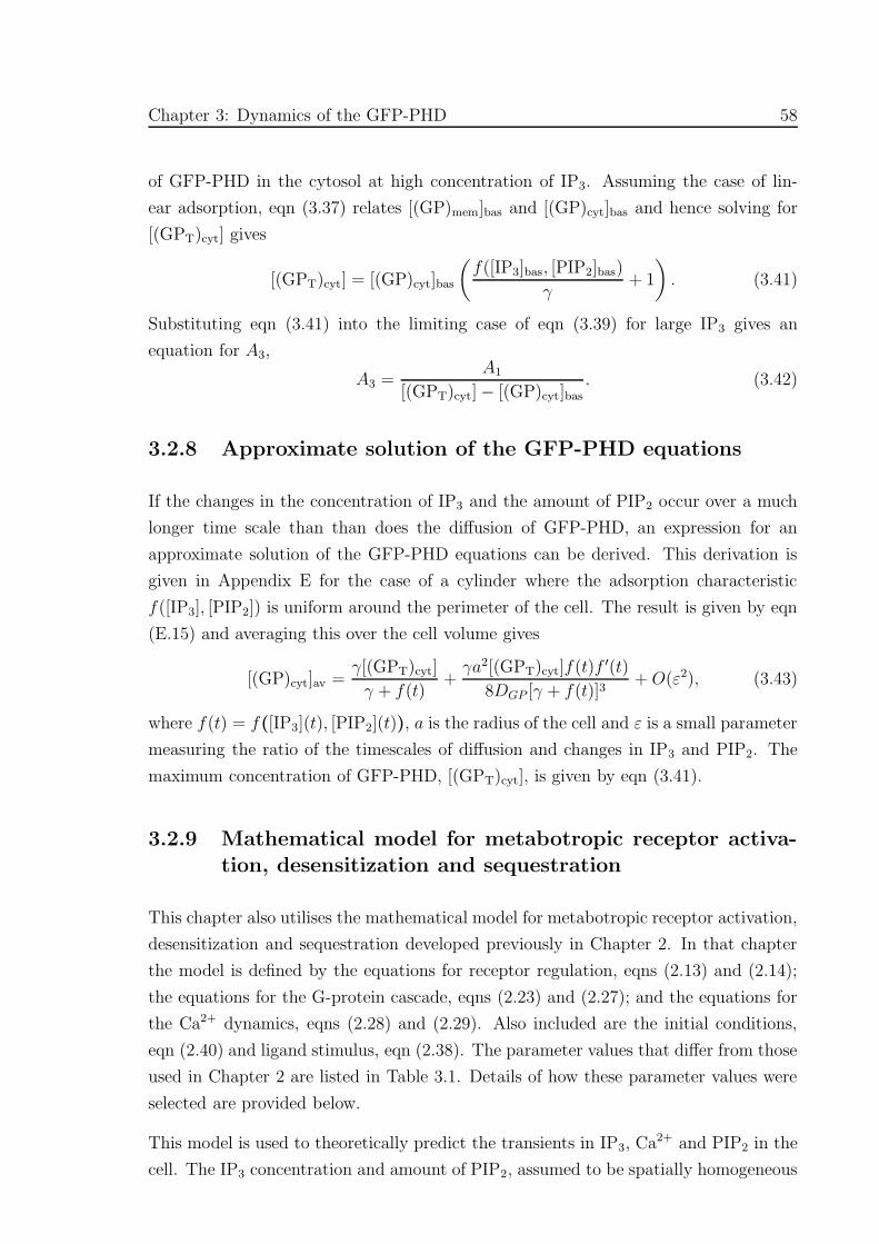
Chapter 3: Dynamics of the GFP-PHD 58
of GFP-PHD in the cytosol at high concentration of IP3. Assuming the case of lin-
ear adsorption, eqn (3.37) relates [(GP)mem]bas and [(GP)cyt]bas and hence solving for
[(GPT)cyt] gives
[(GPT)cyt] = [(GP)cyt]bas
(f([IP3]bas, [PIP2]bas)
γ+ 1
). (3.41)
Substituting eqn (3.41) into the limiting case of eqn (3.39) for large IP3 gives an
equation for A3,
A3 =A1
[(GPT)cyt] − [(GP)cyt]bas
. (3.42)
3.2.8 Approximate solution of the GFP-PHD equations
If the changes in the concentration of IP3 and the amount of PIP2 occur over a much
longer time scale than than does the diffusion of GFP-PHD, an expression for an
approximate solution of the GFP-PHD equations can be derived. This derivation is
given in Appendix E for the case of a cylinder where the adsorption characteristic
f([IP3], [PIP2]) is uniform around the perimeter of the cell. The result is given by eqn
(E.15) and averaging this over the cell volume gives
[(GP)cyt]av =γ[(GPT)cyt]
γ + f(t)+γa2[(GPT)cyt]f(t)f ′(t)
8DGP [γ + f(t)]3+ O(ε2), (3.43)
where f(t) = f([IP3](t), [PIP2](t)), a is the radius of the cell and ε is a small parameter
measuring the ratio of the timescales of diffusion and changes in IP3 and PIP2. The
maximum concentration of GFP-PHD, [(GPT)cyt], is given by eqn (3.41).
3.2.9 Mathematical model for metabotropic receptor activa-tion, desensitization and sequestration
This chapter also utilises the mathematical model for metabotropic receptor activation,
desensitization and sequestration developed previously in Chapter 2. In that chapter
the model is defined by the equations for receptor regulation, eqns (2.13) and (2.14);
the equations for the G-protein cascade, eqns (2.23) and (2.27); and the equations for
the Ca2+ dynamics, eqns (2.28) and (2.29). Also included are the initial conditions,
eqn (2.40) and ligand stimulus, eqn (2.38). The parameter values that differ from those
used in Chapter 2 are listed in Table 3.1. Details of how these parameter values were
selected are provided below.
This model is used to theoretically predict the transients in IP3, Ca2+ and PIP2 in the
cell. The IP3 concentration and amount of PIP2, assumed to be spatially homogeneous
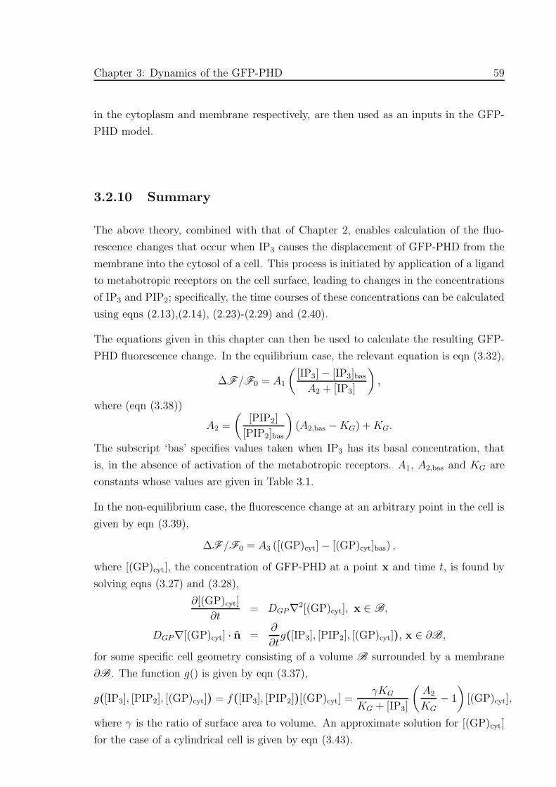
Chapter 3: Dynamics of the GFP-PHD 59
in the cytoplasm and membrane respectively, are then used as an inputs in the GFP-
PHD model.
3.2.10 Summary
The above theory, combined with that of Chapter 2, enables calculation of the fluo-
rescence changes that occur when IP3 causes the displacement of GFP-PHD from the
membrane into the cytosol of a cell. This process is initiated by application of a ligand
to metabotropic receptors on the cell surface, leading to changes in the concentrations
of IP3 and PIP2; specifically, the time courses of these concentrations can be calculated
using eqns (2.13),(2.14), (2.23)-(2.29) and (2.40).
The equations given in this chapter can then be used to calculate the resulting GFP-
PHD fluorescence change. In the equilibrium case, the relevant equation is eqn (3.32),
∆F/F0 = A1
([IP3] − [IP3]bas
A2 + [IP3]
),
where (eqn (3.38))
A2 =
([PIP2]
[PIP2]bas
)(A2,bas −KG) +KG.
The subscript ‘bas’ specifies values taken when IP3 has its basal concentration, that
is, in the absence of activation of the metabotropic receptors. A1, A2,bas and KG are
constants whose values are given in Table 3.1.
In the non-equilibrium case, the fluorescence change at an arbitrary point in the cell is
given by eqn (3.39),
∆F/F0 = A3 ([(GP)cyt] − [(GP)cyt]bas) ,
where [(GP)cyt], the concentration of GFP-PHD at a point x and time t, is found by
solving eqns (3.27) and (3.28),
∂[(GP)cyt]
∂t= DGP∇2[(GP)cyt], x ∈ B,
DGP∇[(GP)cyt] · n =∂
∂tg([IP3], [PIP2], [(GP)cyt]), x ∈ ∂B,
for some specific cell geometry consisting of a volume B surrounded by a membrane
∂B. The function g() is given by eqn (3.37),
g([IP3], [PIP2], [(GP)cyt]) = f([IP3], [PIP2])[(GP)cyt] =γKG
KG + [IP3]
(A2
KG− 1
)[(GP)cyt],
where γ is the ratio of surface area to volume. An approximate solution for [(GP)cyt]
for the case of a cylindrical cell is given by eqn (3.43).

Chapter 3: Dynamics of the GFP-PHD 60
3.3 Results
3.3.1 Model predictions for desensitization based on fluores-
cence data
Figure 3.3 shows the experimental and theoretical equilibrium relative change in flu-
orescence, ∆F/F0, as a function of IP3 concentration. The points are experimental
data taken from Fig. 2D of Hirose et al. (1999) where MDCK cells were injected with
IP3. The solid curve is a plot of eqn (3.32) where the (unstimulated) cell being injected
is assumed to have a fixed basal level of PIP2, hence A2 = A2,bas. The values of A1 and
A2,bas (see Table 3.1) were determined from a least squares fit to the experimental data
using the MATLAB function lsqcurvefit. It is assumed that these parameters remain
valid for the agonist stimulated cells. The basal IP3 concentration, [IP3]bas = 10 nM,
used in eqn (3.32), being much smaller than the range of IP3 concentration used in the
experiments, does not significantly affect the values of A1 and A2,bas.
The time courses of relative fluorescence change in response to an application of 3 µM
of ATP is shown in Fig. 3.4. The solid and dashed curves are theoretical transients
obtained by solving eqns (2.13),(2.14) and (2.23)-(2.29) with initial conditions eqn
(2.40) and ligand stimulus eqn (2.38). The parameter values used are listed in Table
3.1 and rr = 10 s−1. ∆F/F0 was computed from the theoretical transients in IP3
and PIP2, using eqns (3.32) and (3.38). The data points in this figure are taken from
Hirose et al. (1999), Fig. 3B (black curve, no Ca2+ influx) and show the results of an
experiment on permeabilized cells. Permeabilization of the plasma membrane allows
the control of the cytosolic Ca2+ concentration by manipulation of the external Ca2+
concentration. It is assumed that the normal mechanisms of Ca2+ regulation (in this
case the IP3 channels, pumps and leak) are inhibited and have no affect on cytosolic
Ca2+ concentration. It is also assumed that permeabilization has no affect on any of
the signal transduction mechanisms in the cell membrane. The solid curve in Fig. 3.4
shows the theoretical transient in ∆F/F0 for the case where the Ca2+ concentration
has been held at a constant value of 50 nM, this value being taken from the dashed
black line in Hirose et al. (1999), Fig. 3B. The dashed line in Fig. 3.4 indicates
the corresponding result for non-permeabilized cells where the full Ca2+ dynamics are
included. The larger peak in ∆F/F0 and hence larger peak in IP3 concentration for
the non-permeabilized cell case is due to the increased activation of PLC by the higher
(basal and peak) concentration of Ca2+.
In Fig. 3.5 the case where the diffusion of GFP-PHD is assumed to be instantaneous
is compared to cases where GFP-PHD has a finite diffusion rate, for cylindrical and

Chapter 3: Dynamics of the GFP-PHD 61
0 50 100 150 2000
0.1
0.2
0.3
0.4
0.5
0.6
0.7
0.8
0.9
1
IP3 concentration (µM)
∆ F
/F0
ExperimentalTheoretical
Figure 3.3: The equilibrium relative change in fluorescence as a function of IP3 concen-tration in a single cell. The points show experimental values taken from Hirose et al.
(1999), Fig. 2D. The theoretical curve was calculated using eqn (3.32) with the valuesof A1 and A2,bas given in Table 3.1, this latter choice giving the least squares fit of eqn(3.32) to the experimental data.
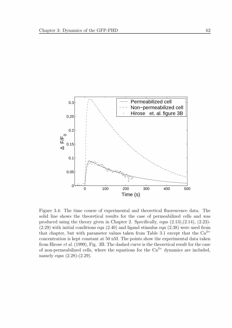
Chapter 3: Dynamics of the GFP-PHD 62
0 100 200 300 400 5000
0.05
0.1
0.15
0.2
0.25
0.3
∆ F
/F0
Time (s)
Permeabilized cellNon−permeabilized cellHirose et. al. figure 3B
Figure 3.4: The time course of experimental and theoretical fluorescence data. Thesolid line shows the theoretical results for the case of permeabilized cells and wasproduced using the theory given in Chapter 2. Specifically, eqns (2.13),(2.14), (2.23)-(2.29) with initial conditions eqn (2.40) and ligand stimulus eqn (2.38) were used fromthat chapter, but with parameter values taken from Table 3.1 except that the Ca2+
concentration is kept constant at 50 nM. The points show the experimental data takenfrom Hirose et al. (1999), Fig. 3B. The dashed curve is the theoretical result for the caseof non-permeabilized cells, where the equations for the Ca2+ dynamics are included,namely eqns (2.28)-(2.29).
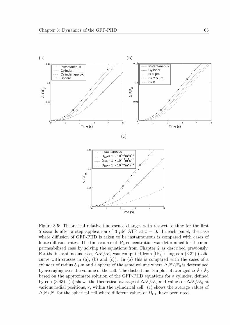
Chapter 3: Dynamics of the GFP-PHD 63
(a) (b)
0 1 2 3 4 50
0.05
0.1
0.15
Time (s)
∆ F
/F0
InstantaneousCylinderCylinder approx.Sphere
0 1 2 3 4 50
0.05
0.1
0.15
Time (s)∆
F/F
0
InstantaneousCylinderr= 5 µmr = 2.5 µmr = 0
(c)
0 1 2 3 4 50
0.05
0.1
0.15
Time (s)
∆ F
/F0
InstantaneousDGP = 1 × 10⁻¹²m2s−1
DGP = 1 × 10⁻¹¹m2s−1
DGP = 1 × 10⁻¹⁰m2s−1
Figure 3.5: Theoretical relative fluoresence changes with respect to time for the first5 seconds after a step application of 3 µM ATP at t = 0. In each panel, the casewhere diffusion of GFP-PHD is taken to be instantaneous is compared with cases offinite diffusion rates. The time course of IP3 concentration was determined for the non-permeabilized case by solving the equations from Chapter 2 as described previously.For the instantaneous case, ∆F/F0 was computed from [IP3] using eqn (3.32) (solidcurve with crosses in (a), (b) and (c)). In (a) this is compared with the cases of acylinder of radius 5 µm and a sphere of the same volume where ∆F/F0 is determinedby averaging over the volume of the cell. The dashed line is a plot of averaged ∆F/F0
based on the approximate solution of the GFP-PHD equations for a cylinder, definedby eqn (3.43). (b) shows the theoretical average of ∆F/F0 and values of ∆F/F0 atvarious radial positions, r, within the cylindrical cell. (c) shows the average values of∆F/F0 for the spherical cell where different values of DGP have been used.
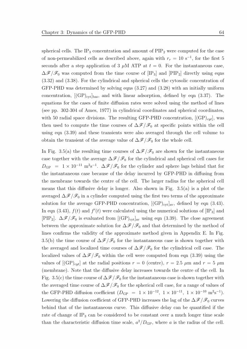
Chapter 3: Dynamics of the GFP-PHD 64
spherical cells. The IP3 concentration and amount of PIP2 were computed for the case
of non-permeabilized cells as described above, again with rr = 10 s−1, for the first 5
seconds after a step application of 3 µM ATP at t = 0. For the instantaneous case,
∆F/F0 was computed from the time course of [IP3] and [PIP2] directly using eqns
(3.32) and (3.38). For the cylindrical and spherical cells the cytosolic concentration of
GFP-PHD was determined by solving eqns (3.27) and (3.28) with an initially uniform
concentration, [(GP)cyt]bas, and with linear adsorption, defined by eqn (3.37). The
equations for the cases of finite diffusion rates were solved using the method of lines
(see pp. 302-304 of Ames, 1977) in cylindrical coordinates and spherical coordinates,
with 50 radial space divisions. The resulting GFP-PHD concentration, [(GP)cyt], was
then used to compute the time courses of ∆F/F0 at specific points within the cell
using eqn (3.39) and these transients were also averaged through the cell volume to
obtain the transient of the average value of ∆F/F0 for the whole cell.
In Fig. 3.5(a) the resulting time courses of ∆F/F0 are shown for the instantaneous
case together with the average ∆F/F0 for the cylindrical and spherical cell cases for
DGP = 1 × 10⁻¹¹ m2s−1. ∆F/F0 for the cylinder and sphere lags behind that for
the instantaneous case because of the delay incurred by GFP-PHD in diffusing from
the membrane towards the centre of the cell. The larger radius for the spherical cell
means that this diffusive delay is longer. Also shown in Fig. 3.5(a) is a plot of the
averaged ∆F/F0 in a cylinder computed using the first two terms of the approximate
solution for the average GFP-PHD concentration, [(GP)cyt]av, defined by eqn (3.43).
In eqn (3.43), f(t) and f ′(t) were calculated using the numerical solutions of [IP3] and
[PIP2]. ∆F/F0 is evaluated from [(GP)cyt]av using eqn (3.39). The close agreement
between the approximate solution for ∆F/F0 and that determined by the method of
lines confirms the validity of the approximate method given in Appendix E. In Fig.
3.5(b) the time course of ∆F/F0 for the instantaneous case is shown together with
the averaged and localized time courses of ∆F/F0 for the cylindrical cell case. The
localized values of ∆F/F0 within the cell were computed from eqn (3.39) using the
values of [(GP)cyt] at the radial positions r = 0 (centre), r = 2.5 µm and r = 5 µm
(membrane). Note that the diffusive delay increases towards the centre of the cell. In
Fig. 3.5(c) the time course of ∆F/F0 for the instantaneous case is shown together with
the averaged time course of ∆F/F0 for the spherical cell case, for a range of values of
the GFP-PHD diffusion coefficient (DGP = 1 × 10⁻¹², 1 × 10⁻¹¹, 1 × 10⁻¹⁰ m2s−1).
Lowering the diffusion coefficient of GFP-PHD increases the lag of the ∆F/F0 curves
behind that of the instantaneous curve. This diffusive delay can be quantified if the
rate of change of IP3 can be considered to be constant over a much longer time scale
than the characteristic diffusion time scale, a2/DGP, where a is the radius of the cell.
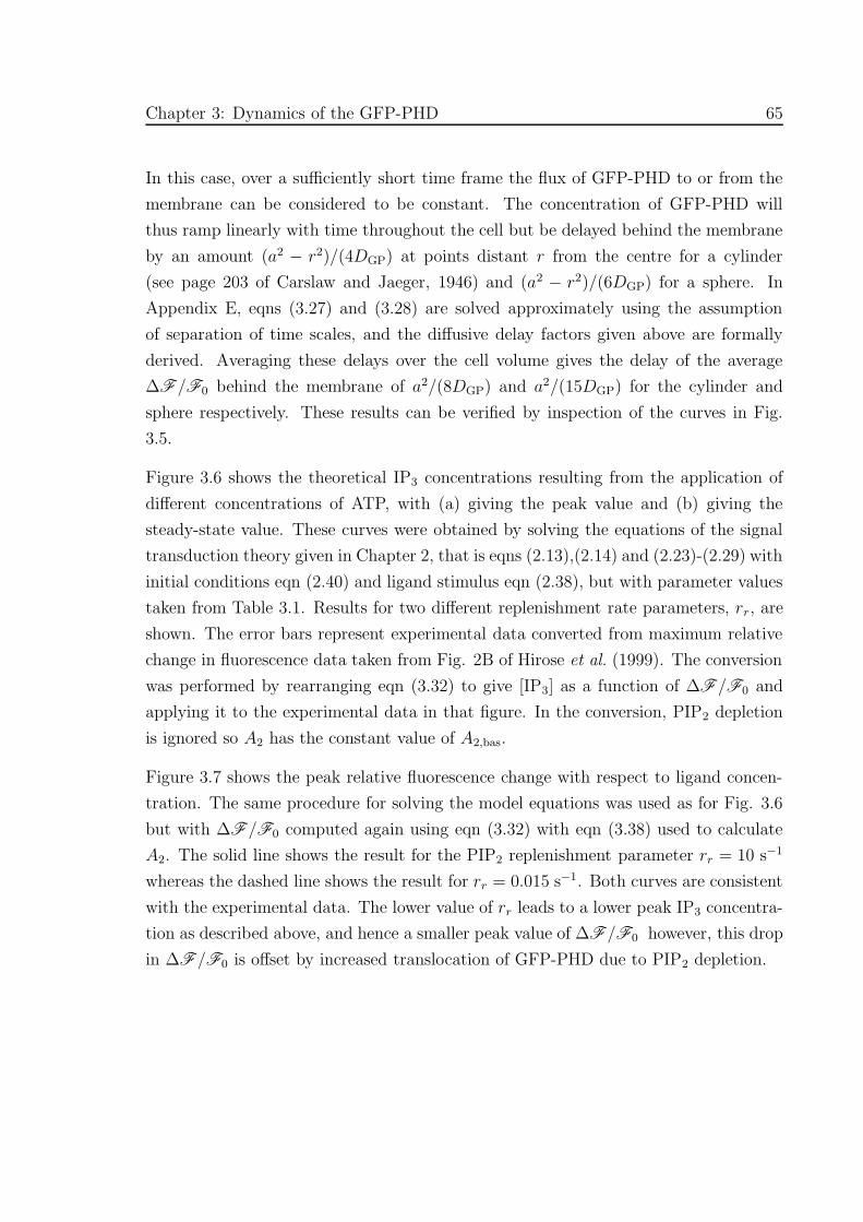
Chapter 3: Dynamics of the GFP-PHD 65
In this case, over a sufficiently short time frame the flux of GFP-PHD to or from the
membrane can be considered to be constant. The concentration of GFP-PHD will
thus ramp linearly with time throughout the cell but be delayed behind the membrane
by an amount (a2 − r2)/(4DGP) at points distant r from the centre for a cylinder
(see page 203 of Carslaw and Jaeger, 1946) and (a2 − r2)/(6DGP) for a sphere. In
Appendix E, eqns (3.27) and (3.28) are solved approximately using the assumption
of separation of time scales, and the diffusive delay factors given above are formally
derived. Averaging these delays over the cell volume gives the delay of the average
∆F/F0 behind the membrane of a2/(8DGP) and a2/(15DGP) for the cylinder and
sphere respectively. These results can be verified by inspection of the curves in Fig.
3.5.
Figure 3.6 shows the theoretical IP3 concentrations resulting from the application of
different concentrations of ATP, with (a) giving the peak value and (b) giving the
steady-state value. These curves were obtained by solving the equations of the signal
transduction theory given in Chapter 2, that is eqns (2.13),(2.14) and (2.23)-(2.29) with
initial conditions eqn (2.40) and ligand stimulus eqn (2.38), but with parameter values
taken from Table 3.1. Results for two different replenishment rate parameters, rr, are
shown. The error bars represent experimental data converted from maximum relative
change in fluorescence data taken from Fig. 2B of Hirose et al. (1999). The conversion
was performed by rearranging eqn (3.32) to give [IP3] as a function of ∆F/F0 and
applying it to the experimental data in that figure. In the conversion, PIP2 depletion
is ignored so A2 has the constant value of A2,bas.
Figure 3.7 shows the peak relative fluorescence change with respect to ligand concen-
tration. The same procedure for solving the model equations was used as for Fig. 3.6
but with ∆F/F0 computed again using eqn (3.32) with eqn (3.38) used to calculate
A2. The solid line shows the result for the PIP2 replenishment parameter rr = 10 s−1
whereas the dashed line shows the result for rr = 0.015 s−1. Both curves are consistent
with the experimental data. The lower value of rr leads to a lower peak IP3 concentra-
tion as described above, and hence a smaller peak value of ∆F/F0 however, this drop
in ∆F/F0 is offset by increased translocation of GFP-PHD due to PIP2 depletion.
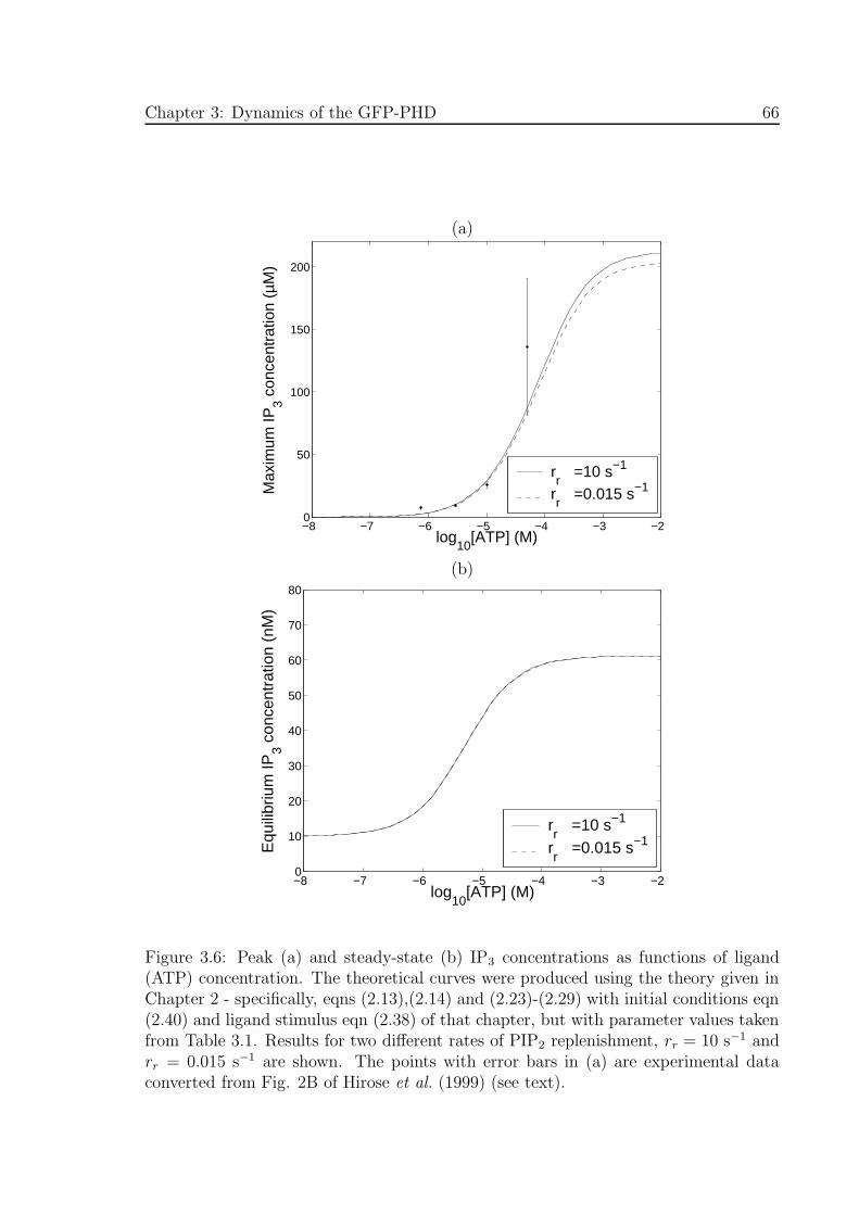
Chapter 3: Dynamics of the GFP-PHD 66
(a)
−8 −7 −6 −5 −4 −3 −20
50
100
150
200
log10
[ATP] (M)
Max
imum
IP3 c
once
ntra
tion
(µM
)
rr
=10 s−1
rr
=0.015 s−1
(b)
−8 −7 −6 −5 −4 −3 −20
10
20
30
40
50
60
70
80
log10
[ATP] (M)
Equ
ilibr
ium
IP3 c
once
ntra
tion
(nM
)
rr
=10 s−1
rr
=0.015 s−1
Figure 3.6: Peak (a) and steady-state (b) IP3 concentrations as functions of ligand(ATP) concentration. The theoretical curves were produced using the theory given inChapter 2 - specifically, eqns (2.13),(2.14) and (2.23)-(2.29) with initial conditions eqn(2.40) and ligand stimulus eqn (2.38) of that chapter, but with parameter values takenfrom Table 3.1. Results for two different rates of PIP2 replenishment, rr = 10 s−1 andrr = 0.015 s−1 are shown. The points with error bars in (a) are experimental dataconverted from Fig. 2B of Hirose et al. (1999) (see text).
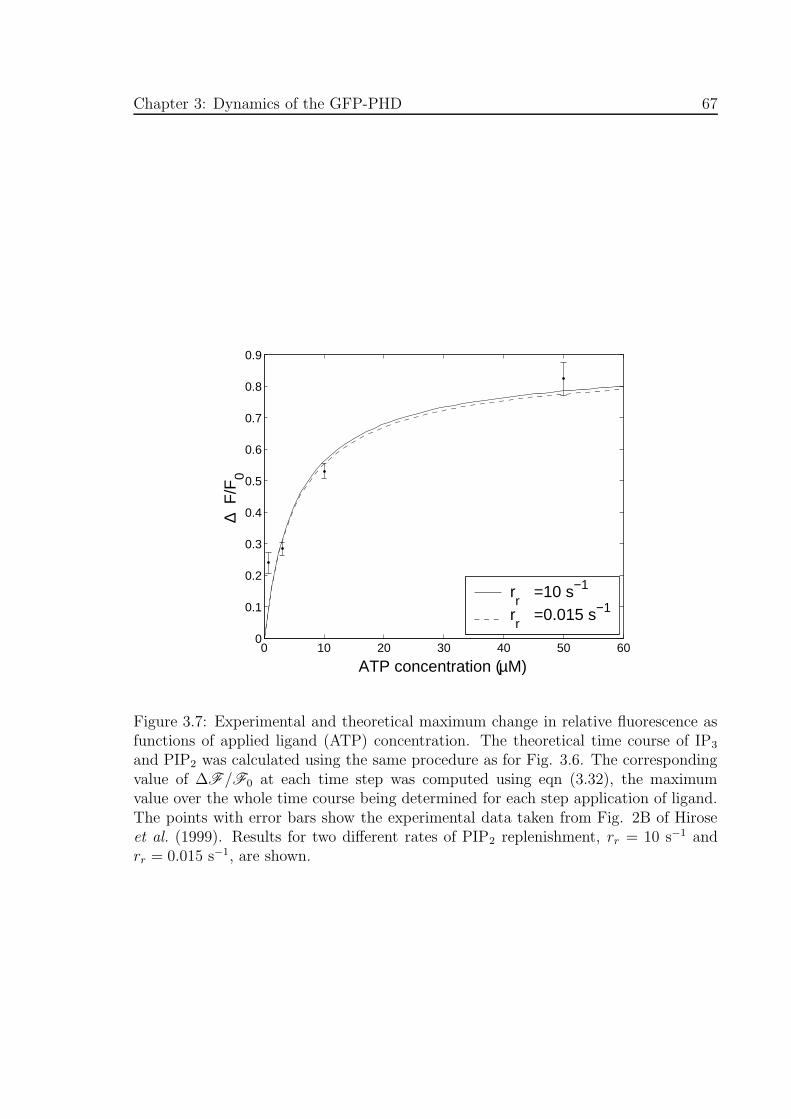
Chapter 3: Dynamics of the GFP-PHD 67
0 10 20 30 40 50 600
0.1
0.2
0.3
0.4
0.5
0.6
0.7
0.8
0.9
ATP concentration (µM)
∆ F
/F0
rr
=10 s−1
rr
=0.015 s−1
Figure 3.7: Experimental and theoretical maximum change in relative fluorescence asfunctions of applied ligand (ATP) concentration. The theoretical time course of IP3
and PIP2 was calculated using the same procedure as for Fig. 3.6. The correspondingvalue of ∆F/F0 at each time step was computed using eqn (3.32), the maximumvalue over the whole time course being determined for each step application of ligand.The points with error bars show the experimental data taken from Fig. 2B of Hiroseet al. (1999). Results for two different rates of PIP2 replenishment, rr = 10 s−1 andrr = 0.015 s−1, are shown.
Chapter 3: Dynamics of the GFP-PHD 68
3.3.2 Parameter value selection
The parameter values for the model equations presented in Chapter 2, chosen for the
case of MDCK cells, as well as the parameter values for the GFP-PHD dynamics are
listed in Table 3.1. Only those parameter values that differ from those given in Table
2.1 are listed.
For the MDCK cell a diameter of 10 µm and a volume of 8 × 10⁻¹⁵ m3 were chosen
based on the images of the cells in Fig. 4 of Hirose et al. (1999). The diameter of the
spherical cell, approximately 21.22 µm, was chosen so as to have the same volume as
the cylindrical cell. This ensures that, with all the other signal transduction parameters
the same, both types of cell will have the same second messenger response under the
same stimulus conditions.
The numerical value of the parameter A3 appearing in eqn (3.39) was computed from
the values of [(GP)cyt], [IP3]bas and γ provided in Table 3.1 hence eqn (3.39) becomes
∆F/F0 = 2348.8×([(GP)cyt] − 2 × 10⁻⁶
)for both the cylindrical and spherical cells.
The values used for the GFP-PHD diffusion coefficient (DGP = 1 × 10⁻¹², 1 ×10⁻¹¹, 1× 10⁻¹⁰ m2s−1) were chosen to give a broad range of possible values and were
chosen to be inclusive of results quoted by Dayel et al. (1999) for the bulk diffusion
coefficient of the isolated GFP in the cytoplasm of CHO cells.
A definite value for K1 is not available but a larger value of K1 than that used in
Chapter 2 is required for curve fitting in Figs. 3.4 and 3.7 (note that dissociation
constants for different ligands can differ markedly for the same type of receptor). The
ratio K1/K2 was kept the same as in Chapter 2. The values of kr and ke were adjusted
from those used in Chapter 2 so that the steady-state IP3 concentration at saturating
levels of ligand matches that predicted in that chapter, approximately 60 nM.
The value of [GT ] was selected to give a basal level of activated G-protein, [G]bas,
similar to that in Chapter 2. The value of [PIP2]bas was chosen to be sufficiently large
to give minimal depletion of PIP2 for both values of rr, consistent with the conclusion
of Hirose et al. (1999) that the amount of free PIP2 remains either constant or much
greater than the dissociation constant for PIP2 binding with GFP-PHD.
As in Chapter 2, the numerical values of the parameters η1, η2, η3 and [Ca2+]bas
were chosen to give the desired Ca2+ transient characteristics. As before the desired
basal Ca2+ concentration was approximately 100 nM (taken from Fig. 3A of Hirose
et al., 1999) but here the maximum desired Ca2+ change was approximately 400 nM
(estimated again from Fig. 3A of Hirose et al., 1999).

Chapter 3: Dynamics of the GFP-PHD 69
The values of α and Kc were determined by simultaneously obtaining a best fit for the
theoretical curve to the experimental data in Fig. 3.7 while obtaining a fit for the peak
of the theoretical curve to the data for the permeabilized cell case in Fig. 3.4. For this
same curve, the value of kp was chosen to fit the decaying part of the experimental
data and the GTP-ase rate parameter kd was chosen so that the curve fits the rising
phase of the data.

Chap
ter3:
Dynam
icsof
the
GFP
-PH
D70
Symbol Definition Value Notes
GFP-PHD dynamics
KG Dissociation constant for IP3 binding to GFP-PHD 93 nM Hirose et al. (1999)[(GP)cyt]bas Basal conc. of GFP-PHD 2 µM ”DGP Diffusion coefficient of GFP-PHD 10−12, 10−11 , 10−10 m2s−1 See text.A1 Empirically determined parameter in eqn (3.32) 0.9767 ”A2,bas ” (for basal PIP2 levels) 21.52 µM ”
A3 Empirically determined parameter in eqn (3.39) 2348.8 M−1 ”
Receptor regulation
K1 Unphosphorylated receptor dissociation constant 500 µM See text.K2 Phosphorylated receptor dissociation constant 0.01 M ”kr Receptor recycling rate 5.83 × 10⁻⁵ s−1 ”kp Receptor phosphorylation rate 0.85 s−1 ”[RT ], ke, ξ see Table 2.1
G protein cascade
[GT ] Total number of G-protein molecules 1 × 10⁷ See text.ka G-protein activation rate 0.017 s−1 ”kd G-protein deactivation rate 0.15 s−1 ”[(PIP2)T] Total number of PIP2 molecules 5.0 × 10⁷ ”
rr PIP2 replenishment rate 10, 0.015 s−1 ”δ G-protein intrinsic activity parameter 1.385, 1.385 × 10⁻⁵ ”Kc Dissociation constant for Ca2+ binding to PLC 0.4 µM ”α Effective signal gain parameter 3.847 × 10⁻⁷ s−1 ”ν Cell volume 8 × 10⁻¹⁵ m3 ”kdeg , Na see Table 2.1
Ca2+ dynamics
η1 Effective IP3 channel permeability 133 s−1 See text.η2 Effective ER leak permeability 2.72 s−1 ”η3 Effective Ca2+ pump permeability 45 µMs−1 ”[(Ca2+)T] Total conc. of Ca2+ 1 mM ”εr, d1, d2, d3, d5, a2
[Be], Ke, [Bx], Kx
[BER], KER, k3 see Table 2.1
Equilibrium values for rr = 10 s−1
[G]bas Basal no. of active G-protein molecules 16 See text.[PIP2]bas Basal no. of PIP2 molecules 4999995 ”[IP3]bas Basal IP3 conc. 10 nM ”[Ca2+]bas Basal Ca2+ conc. 100.4 nM ”hbas Basal fraction of active IP3 channels 0.6055 ”
Table 3.1: Model parameter values.
Chapter 3: Dynamics of the GFP-PHD 71
Discussion
In this chapter a mathematical model has been developed for the translocation of
GFP-PHD between the membrane and cytosol of a cell in the presence of IP3. The
model has been successfully used in conjunction with a model for metabotropic receptor
activation, desensitization and sequestration (Chapter 2) to quantify experimental data
for the purinergic stimulation of MDCK cells.
A central result of the present work is the formal derivation of an expression for the
relative fluoresence change (∆F/F0) as a function of IP3 under equilibrium conditions
(eqn (3.32)). This formula, with parameters determined experimentally, was then
used to quantify IP3 concentrations for other experimental data (so as to determine
parameters in the signal transduction model). Using this procedure it was deduced
that the maximum IP3 concentration in these cells reached hundreds of µM. This is
credible given the evidence suggesting that IP3 concentration can reach tens of µM in
some cells (Horstman et al., 1988; Khodakhah et al., 1993; Luzzi et al., 1998).
There are several assumptions and considerations that need to be examined carefully
if one wishes to use this mathematical model of the dynamics of the GFP-PHD for
comparison with the results of experimental work. One assumption, used for sim-
plifying the model equations, is that the concentrations of GFP-PHD, PIP2 and IP3
are uniform around the perimeter of the cell. However, a heterogeneous distribution
of membrane components such as receptor patches which can occur in cells expressing
P2Y2 receptors (Sromek and Harden, 1998) or PIP2 (Pike and Casey, 1996) would cause
spatially-dependent generation of IP3. In these cases, there would be non-uniform rates
of GFP-PHD translocation across the membrane and there is evidence of this in Fig.
4 of Hirose et al. (1999). The equations for the dynamics of the GFP-PHD at a point
on the membrane (eqns (3.27) and (3.28)) are still valid in these cases.
Depletion of PIP2 levels also causes translocation of GFP-PHD into the cytosol. In this
study the level of PIP2 and its rate of resupply have been chosen to give low depletion
of PIP2 during agonist stimulation, consistent with the experimental evidence. PIP2
depletion may be significant in some cells to which the GFP-PHD probe technique has
been applied (Varnai and Balla, 1998), in which case this technique would have to be
used in conjunction with some method of monitoring PIP2 levels. Fluorescent-labeled
neomycin has been suggested as a probe for PIP2 levels in membranes (Arbuzova et
al., 2000).
The assumption of rapid binding of IP3 and PIP2 with GFP-PHD allows the full
equations (eqns (3.1)-(3.8)) to be simplified to a single equation describing the diffusion

Chapter 3: Dynamics of the GFP-PHD 72
of GFP-PHD (eqn (3.27)) and a boundary condition (eqn (3.28)). Some experimental
credence for this assumption can be found in the paper by Hirose et al. (1999). There,
changes in cytosolic and membrane fluorescence for the case of Ca2+ waves (see their
Fig. 4) are observed to lag the corresponding Ca2+ concentration changes by an amount
in the order of seconds. This is consistent with the model predictions described in the
results section.
The method of imaging IP3 using GFP-PHD is quite unlike conventional Ca2+ indica-
tors. The latter indicate local Ca2+ in the cytoplasm and their fluorescence properties
are changed by the binding of Ca2+; for example, for fura-2 there is a shift in the
absorption spectra to a shorter wavelength. In contrast, changes in the fluorescence
intensity of GFP-PHD in the cytosol are due to changes in the cytosolic concentration
of GFP-PHD.
Because GFP-PHD dissociates and reassociates at the membrane, strictly speaking the
probe measures changes in IP3 occurring at the membrane. Changes to the concentra-
tion of GFP-PHD inside the cytosol are delayed due to the finite rate of diffusion. This
delay is likely to be of the order of hundreds of milliseconds, depending on the precise
value of the diffusion coefficient and the dimensions of the cell (see Fig. 3.5). This
implies a limit to the resolution of fast events, for example Ca2+-IP3 waves, if they are
observed by averaging relative changes in fluorescence over the whole cell interior. Over
sufficiently long times, such as the time scale of desensitization of the P2Y2 receptors,
this complication can be ignored and the GFP-PHD in the cytosol can be considered
to be in equilibrium with that bound to the membrane.
Saturation of the curves shown in Fig. 3.7 is due to maximal release of GFP-PHD into
the cytosol rather than to saturation of the receptors by ligand, the latter occurring
at concentrations greater than about 1 mM ATP (see Fig. 3.6(a)). Hence, saturation
of the GFP-PHD system may pose a problem in estimating large IP3 concentrations
(hence the large error bar in Fig. 3.6(a)), and yet for concentrations of the order of
several micromolar the relation between IP3 and cytosolic GFP-PHD fluorescence can
be taken as linear (see Fig. 3.3).
An interesting aspect of the work of Hirose et al. (1999) is the possibility of Ca2+-IP3
waves and oscillations (see their Figs. 3A and Fig. 4). The model for the dynamics
of GFP-PHD given in this chapter together with the model for Ca2+ and IP3 changes
due to metabotropic receptor activity in Chapter 2 could be used to study these phe-
nomema. The signal transduction model can exhibit oscillations with the appropriate
choice of parameter values but would have to be extended to include diffusion of IP3
and Ca2+ for the case of Ca2+-IP3 waves.
73
Chapter 4
Fire-Diffuse-Fire calcium waves inconfined intracellular spaces
In this chapter the propagation of Fire-Diffuse-Fire (FDF) Ca2+ waves through a three
dimensional rectangular domain is considered. The domain is infinite in extent in
the direction of propagation but with lateral barriers to diffusion which contain Ca2+
pumps. The Ca2+ concentration profile due to the firing of a release site (spark) is
derived analytically based on the Green’s function for the diffusion equation on the
domain. The existence, stability and speed of these waves is shown to be critically
dependent on the dimensions of the domain and the Ca2+ pump rate. It is shown
that the smaller the dimensions of the region, the lower the Ca2+ release flux required
for wave propagation, and the higher the wave speed. Also it is shown that the region
may support multiple Ca2+ wavefronts of varying wave speed. This model is relevant to
subsarcolemmal waves in atrial myocytes (Kockskamper et al., 2001), and the results
may be of importance in understanding the roles of the endoplasmic/sarcoplasmic
reticulum, surface membranes and Ca2+ pumps in the intracellular Ca2+ dynamics of
cells.
4.1 Introduction
Intracellular Ca2+ waves occur in many different cell types including smooth muscle
(Pabelick et al., 1999), cardiac cells (Wussling and Salz, 1996) and Xenopus oocytes
(Fontanilla and Nuccitelli, 1998). These waves arise from the process of calcium in-
duced calcium release (CICR) from channels in the endoplasmic (ER) or sarcoplasmic
reticulum (SR) coupled to the diffusion of Ca2+ in the cytosol.
Ca2+ waves sometimes propagate as a sequence of bursts or ‘sparks’ of Ca2+ from
Chapter 4: Ca2+ waves in confined spaces 74
adjacent clusters of ryanodine channels (RyRs) as in the case of cardiac cells (Lipp et
al., 2002), or as ‘puffs’ of Ca2+ from clusters of inositol trisphosphate (IP3) sensitive
channels in the case of immature Xenopus oocytes (Parker and Yao, 1991; Callamaras
et al., 1998).
Experiments show that Ca2+ sparks are localized in regions close to the sarcolemma
(SL) in both smooth muscle cells (Perez et al., 1999; Jaggar et al., 2000) and cardiac
myocytes (Blatter, 1997; Niggli, 1999). In both these cell types the SL is known to
be in close proximity to parts of the SR, forming a restricted subsarcolemmal space in
which diffusion of Ca2+ occurs.
In the case of atrial myocytes, Ca2+ entering the cell via an L-type channel may trigger
an apposite cluster of ryanodine channels on the SR. The resulting release of Ca2+,
diffusing through the subsarcolemmal space can trigger further sparks and Ca2+ waves;
see Fig. 1.7. This subsarcolemmal wave precedes Ca2+ release in the central part of
the cell. In other cell types, for example the rat megakaryocyte (Thomas et al., 2001),
Xenopus laevis egg (Fontanilla and Nuccitelli, 1998), and vascular endothelial cells
(Huser and Blatter, 1997), Ca2+ waves in the peripheral regions of the cell have been
observed to precede waves in the central parts of the cell and travel with a greater
speed.
A theoretical study of the propagation of Ca2+ waves due to Ca2+ sparks in confined
diffusion spaces is therefore desirable. An investigation of the effect of obstructed
diffusion of Ca2+ transients in smooth muscle is given in the papers by Kargacin and
Fay (1991) and Kargacin (1994) but these do not include a study of Ca2+ sparks or
waves.
There is however a growing literature concerned with mathematical models for Ca2+
waves arising from sparks. The papers by Keizer et al. (1998), Pearson and Dawson
(1998), and Dawson et al. (1999), use a model comprising a collinear arrangement of
Ca2+ release units (CRUs) coupled by a one-dimensional Ca2+ diffusion model with
linearized buffering. The paper by Coombes (2001) extends the model to include the
effects of removal of Ca2+ by linearized Ca2+ pumps. These models are collectively
known as the Fire-Diffuse-Fire (FDF) model, a term that will be adopted in this
thesis. In the FDF model, a CRU fires when the concentration of Ca2+ at the site
reaches a threshold level, that is, the firing is deterministic. Also, once a site fires it
is assumed to remain in a refractory period indefinitely and is unable to re-fire. The
paper by Keizer and Smith (1998) modifies the FDF model by using a stochastic model
for the Ca2+ release site, based on the kinetics of isolated Ryanodine channels (Gyorke
and Fill, 1993). This allows simulations of terminating and re-starting Ca2+ waves,

Chapter 4: Ca2+ waves in confined spaces 75
although the detailed behaviour of the Ryanodine channel is not yet well understood
(Sitsapesan and Williams, 2000).
Other authors have developed three-dimensional cell models for Ca2+ waves where
the CRUs are arranged in regular arrays throughout the cell, for example along z-
lines in cardiac myocytes. In the paper by Subramanian et al. (2001), CRU firing is
deterministic whereas in that by Izu et al. (2001), a CRU is assigned a probability
of firing which is an increasing function of Ca2+ concentration. Both models include
anisotropic diffusion of Ca2+ as well as realistic models for Ca2+ buffering and Ca2+
pumps.
There is a corresponding literature devoted to models for Ca2+ waves propagating due
to puffs of Ca2+ from clusters of IP3 receptors located on the SR. The IP3 channel is
sensitive to both IP3 and Ca2+ (Bezprozvanny et al., 1991), and can exhibit both CICR
and IP3 induced Ca2+ release (IICR). Theoretical studies of Ca2+ waves propagating
between release sites in one space dimension are given by Kupferman et al. (1997),
Bugrim et al. (1997) and Falcke et al. (2000).
These models are not wholly suitable to studying FDF waves in confined spaces. The
one-dimensional models lack the necessary additional space dimensions and the three-
dimensional models do not include barriers to diffusion explicitly. In this chapter an
extension of the one-dimensional FDF model to include constrained diffusion in three
space dimensions will be given. Numerical simulations and analytical techniques will
then be used to study the properties of Ca2+ spark induced Ca2+ waves in confined
intracellular spaces.
4.2 Methods
4.2.1 Model for Ca2+ release and uptake
Once the Ca2+ concentration at a site exceeds a fixed concentration, cthr, a release of
Ca2+ into the intracellular space occurs. The release site is then assumed to remain
unable to fire again indefinitely. The case of sparks occurring in an infinite domain B,
shown in Fig. 4.1, is considered.
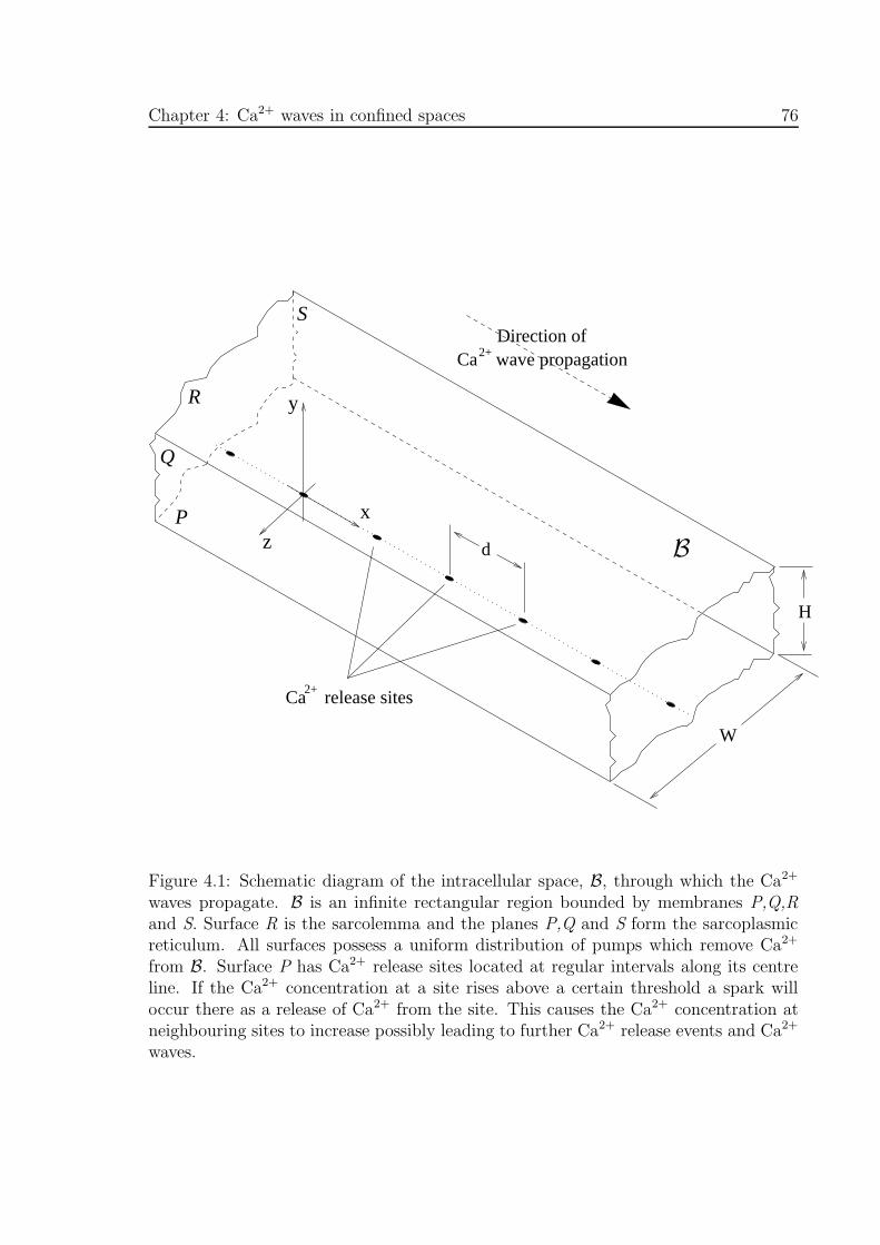
Chapter 4: Ca2+ waves in confined spaces 76
Ca wave propagation
Ca release sites2+
H
2+Direction of
������������������������������������������������������
������������������������������������������������������
P
Q
R
S
y
x
z
W
d B
Figure 4.1: Schematic diagram of the intracellular space, B, through which the Ca2+
waves propagate. B is an infinite rectangular region bounded by membranes P,Q,R
and S. Surface R is the sarcolemma and the planes P,Q and S form the sarcoplasmicreticulum. All surfaces possess a uniform distribution of pumps which remove Ca2+
from B. Surface P has Ca2+ release sites located at regular intervals along its centreline. If the Ca2+ concentration at a site rises above a certain threshold a spark willoccur there as a release of Ca2+ from the site. This causes the Ca2+ concentration atneighbouring sites to increase possibly leading to further Ca2+ release events and Ca2+
waves.
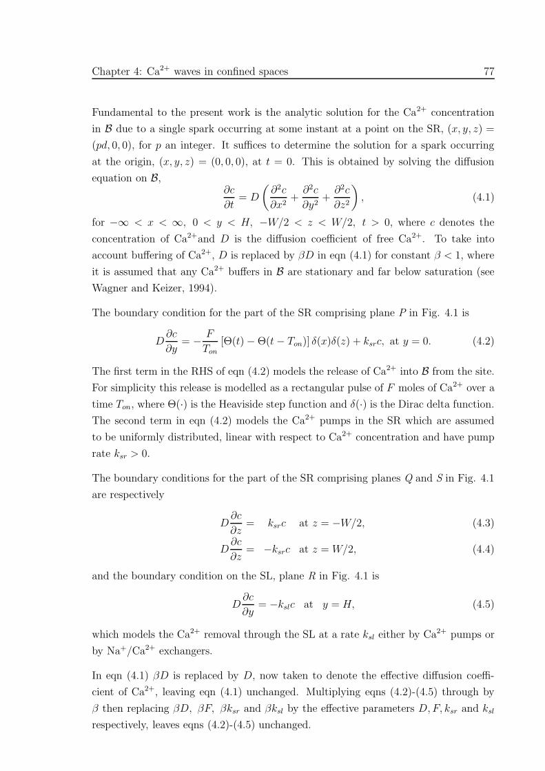
Chapter 4: Ca2+ waves in confined spaces 77
Fundamental to the present work is the analytic solution for the Ca2+ concentration
in B due to a single spark occurring at some instant at a point on the SR, (x, y, z) =
(pd, 0, 0), for p an integer. It suffices to determine the solution for a spark occurring
at the origin, (x, y, z) = (0, 0, 0), at t = 0. This is obtained by solving the diffusion
equation on B,∂c
∂t= D
(∂2c
∂x2+∂2c
∂y2+∂2c
∂z2
), (4.1)
for −∞ < x < ∞, 0 < y < H, −W/2 < z < W/2, t > 0, where c denotes the
concentration of Ca2+and D is the diffusion coefficient of free Ca2+. To take into
account buffering of Ca2+, D is replaced by βD in eqn (4.1) for constant β < 1, where
it is assumed that any Ca2+ buffers in B are stationary and far below saturation (see
Wagner and Keizer, 1994).
The boundary condition for the part of the SR comprising plane P in Fig. 4.1 is
D∂c
∂y= − F
Ton
[Θ(t) − Θ(t− Ton)] δ(x)δ(z) + ksrc, at y = 0. (4.2)
The first term in the RHS of eqn (4.2) models the release of Ca2+ into B from the site.
For simplicity this release is modelled as a rectangular pulse of F moles of Ca2+ over a
time Ton, where Θ(·) is the Heaviside step function and δ(·) is the Dirac delta function.
The second term in eqn (4.2) models the Ca2+ pumps in the SR which are assumed
to be uniformly distributed, linear with respect to Ca2+ concentration and have pump
rate ksr > 0.
The boundary conditions for the part of the SR comprising planes Q and S in Fig. 4.1
are respectively
D∂c
∂z= ksrc at z = −W/2, (4.3)
D∂c
∂z= −ksrc at z = W/2, (4.4)
and the boundary condition on the SL, plane R in Fig. 4.1 is
D∂c
∂y= −kslc at y = H, (4.5)
which models the Ca2+ removal through the SL at a rate ksl either by Ca2+ pumps or
by Na+/Ca2+ exchangers.
In eqn (4.1) βD is replaced by D, now taken to denote the effective diffusion coeffi-
cient of Ca2+, leaving eqn (4.1) unchanged. Multiplying eqns (4.2)-(4.5) through by
β then replacing βD, βF, βksr and βksl by the effective parameters D,F, ksr and ksl
respectively, leaves eqns (4.2)-(4.5) unchanged.
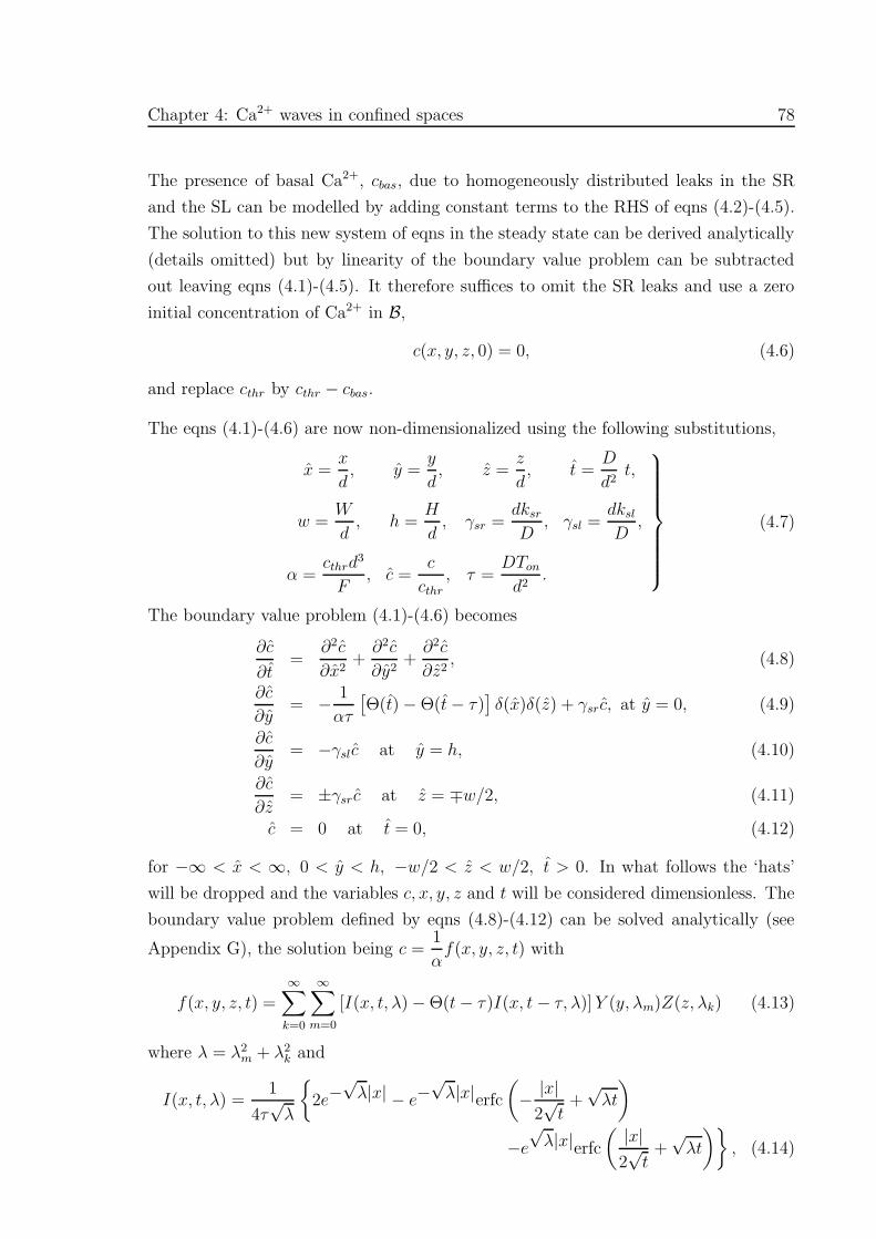
Chapter 4: Ca2+ waves in confined spaces 78
The presence of basal Ca2+, cbas, due to homogeneously distributed leaks in the SR
and the SL can be modelled by adding constant terms to the RHS of eqns (4.2)-(4.5).
The solution to this new system of eqns in the steady state can be derived analytically
(details omitted) but by linearity of the boundary value problem can be subtracted
out leaving eqns (4.1)-(4.5). It therefore suffices to omit the SR leaks and use a zero
initial concentration of Ca2+ in B,
c(x, y, z, 0) = 0, (4.6)
and replace cthr by cthr − cbas.
The eqns (4.1)-(4.6) are now non-dimensionalized using the following substitutions,
x =x
d, y =
y
d, z =
z
d, t =
D
d2t,
w =W
d, h =
H
d, γsr =
dksr
D, γsl =
dksl
D,
α =cthrd
3
F, c =
c
cthr, τ =
DTon
d2.
(4.7)
The boundary value problem (4.1)-(4.6) becomes
∂c
∂t=
∂2c
∂x2+∂2c
∂y2+∂2c
∂z2, (4.8)
∂c
∂y= − 1
ατ
[Θ(t) − Θ(t− τ)
]δ(x)δ(z) + γsrc, at y = 0, (4.9)
∂c
∂y= −γslc at y = h, (4.10)
∂c
∂z= ±γsrc at z = ∓w/2, (4.11)
c = 0 at t = 0, (4.12)
for −∞ < x < ∞, 0 < y < h, −w/2 < z < w/2, t > 0. In what follows the ‘hats’
will be dropped and the variables c, x, y, z and t will be considered dimensionless. The
boundary value problem defined by eqns (4.8)-(4.12) can be solved analytically (see
Appendix G), the solution being c =1
αf(x, y, z, t) with
f(x, y, z, t) =
∞∑
k=0
∞∑
m=0
[I(x, t, λ) − Θ(t− τ)I(x, t− τ, λ)]Y (y, λm)Z(z, λk) (4.13)
where λ = λ2m + λ2
k and
I(x, t, λ) =1
4τ√λ
{2e−
√λ|x| − e−
√λ|x|erfc
(− |x|
2√t
+√λt
)
−e√λ|x|erfc
( |x|2√t
+√λt
)}, (4.14)

Chapter 4: Ca2+ waves in confined spaces 79
Y (y, λm) =4λm cosφm cos(λmy − φm)
2λmh+ sin 2(λmh− φm) + sin 2φm, (4.15)
Z(z, λk) =4λk cos
[λk
w2− φk
]cos[λk(z + w
2) − φk
]
2λkw + sin 2(λkw − φk) + sin 2φk, (4.16)
for −∞ < x < ∞, 0 < y < h, −w/2 < z < w/2, t > 0. In eqn (4.14) erfc(·) is the
complementary error function defined by
erfc(x) =2√π
∫ ∞
x
e−u2
du.
The φm and φk in eqns (4.15) and (4.16) are defined by
tanφm =γsr
λm
, tanφk =γsr
λk
, (4.17)
where for each m, λm satisfies
tanλmh =(γsr + γsl)λm
λ2m − γsrγsl
, (4.18)
and for each k, λk satisfies
tanλkh =2γsrλk
λ2k − γ2
sr
. (4.19)
4.2.2 Existence and stability of Ca2+ waves
If a sequence of sites fire, the resulting Ca2+ concentration at any time, by linearity
of the boundary value problem (4.8)-(4.12), will be the sum of the contributions from
each of the sites that have fired previously. Thus for a sequence of firings at times
{t0, t1, . . . tN−1} at corresponding sites with x-coordinates {x0, x1, . . . xN−1} and with
zero Ca2+ concentration for t < t0, the resulting Ca2+ concentration for t > tN−1 is
c(x, y, z, t) =1
α
N−1∑
p=0
f(x− xp, y, z, t− tp), (4.20)
with f defined by eqns (4.13)-(4.19). The location and time of the next firing is
determined by solving for xN and t in eqn (4.20) such that c(xN , 0, 0, t) = 1. Given
a sequence of N consecutive firings of adjacent sites in the positive x direction it can
be shown that c(x, 0, 0, t) is a monotone decreasing function of x > xN−1 for t > tN−1
fixed. Therefore, the next site that fires must be located at xN = N , so tN is determined
by solving the nonlinear equation
c(N, 0, 0, tN) =1
α
N−1∑
p=0
f((N − p), 0, 0, tN − tp) = 1. (4.21)
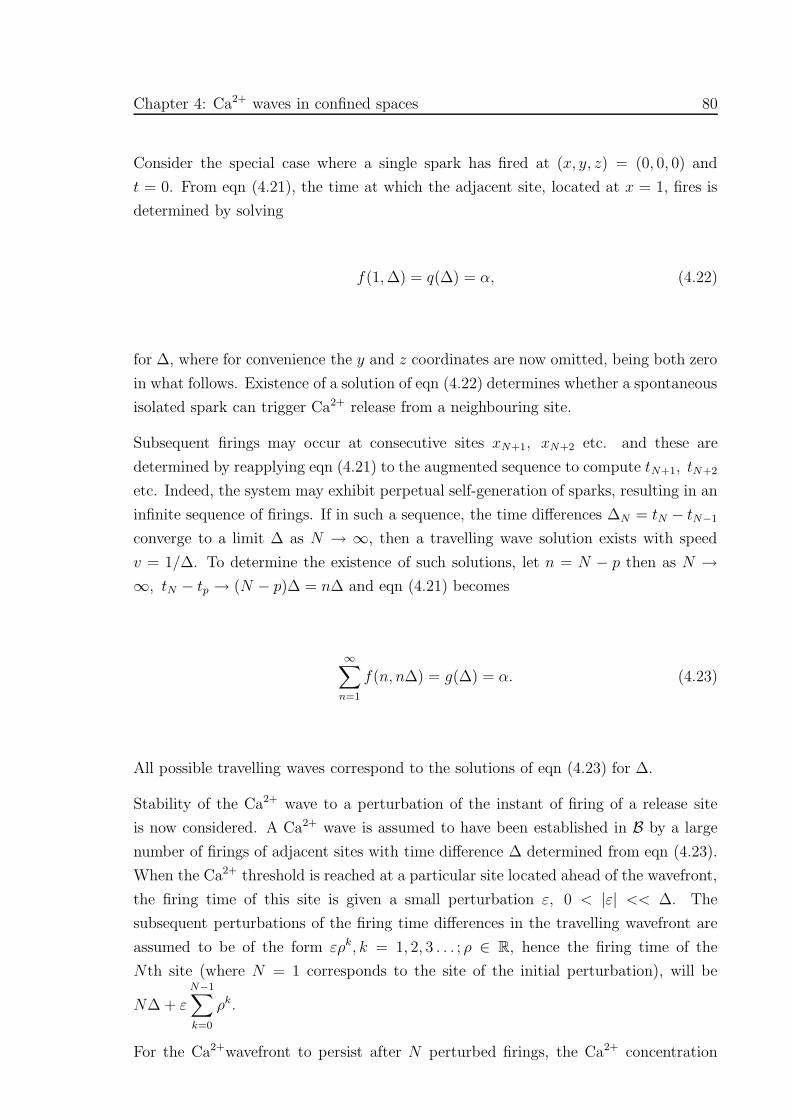
Chapter 4: Ca2+ waves in confined spaces 80
Consider the special case where a single spark has fired at (x, y, z) = (0, 0, 0) and
t = 0. From eqn (4.21), the time at which the adjacent site, located at x = 1, fires is
determined by solving
f(1,∆) = q(∆) = α, (4.22)
for ∆, where for convenience the y and z coordinates are now omitted, being both zero
in what follows. Existence of a solution of eqn (4.22) determines whether a spontaneous
isolated spark can trigger Ca2+ release from a neighbouring site.
Subsequent firings may occur at consecutive sites xN+1, xN+2 etc. and these are
determined by reapplying eqn (4.21) to the augmented sequence to compute tN+1, tN+2
etc. Indeed, the system may exhibit perpetual self-generation of sparks, resulting in an
infinite sequence of firings. If in such a sequence, the time differences ∆N = tN − tN−1
converge to a limit ∆ as N → ∞, then a travelling wave solution exists with speed
v = 1/∆. To determine the existence of such solutions, let n = N − p then as N →∞, tN − tp → (N − p)∆ = n∆ and eqn (4.21) becomes
∞∑
n=1
f(n, n∆) = g(∆) = α. (4.23)
All possible travelling waves correspond to the solutions of eqn (4.23) for ∆.
Stability of the Ca2+ wave to a perturbation of the instant of firing of a release site
is now considered. A Ca2+ wave is assumed to have been established in B by a large
number of firings of adjacent sites with time difference ∆ determined from eqn (4.23).
When the Ca2+ threshold is reached at a particular site located ahead of the wavefront,
the firing time of this site is given a small perturbation ε, 0 < |ε| << ∆. The
subsequent perturbations of the firing time differences in the travelling wavefront are
assumed to be of the form ερk, k = 1, 2, 3 . . . ; ρ ∈ R, hence the firing time of the
Nth site (where N = 1 corresponds to the site of the initial perturbation), will be
N∆ + εN−1∑
k=0
ρk.
For the Ca2+wavefront to persist after N perturbed firings, the Ca2+ concentration
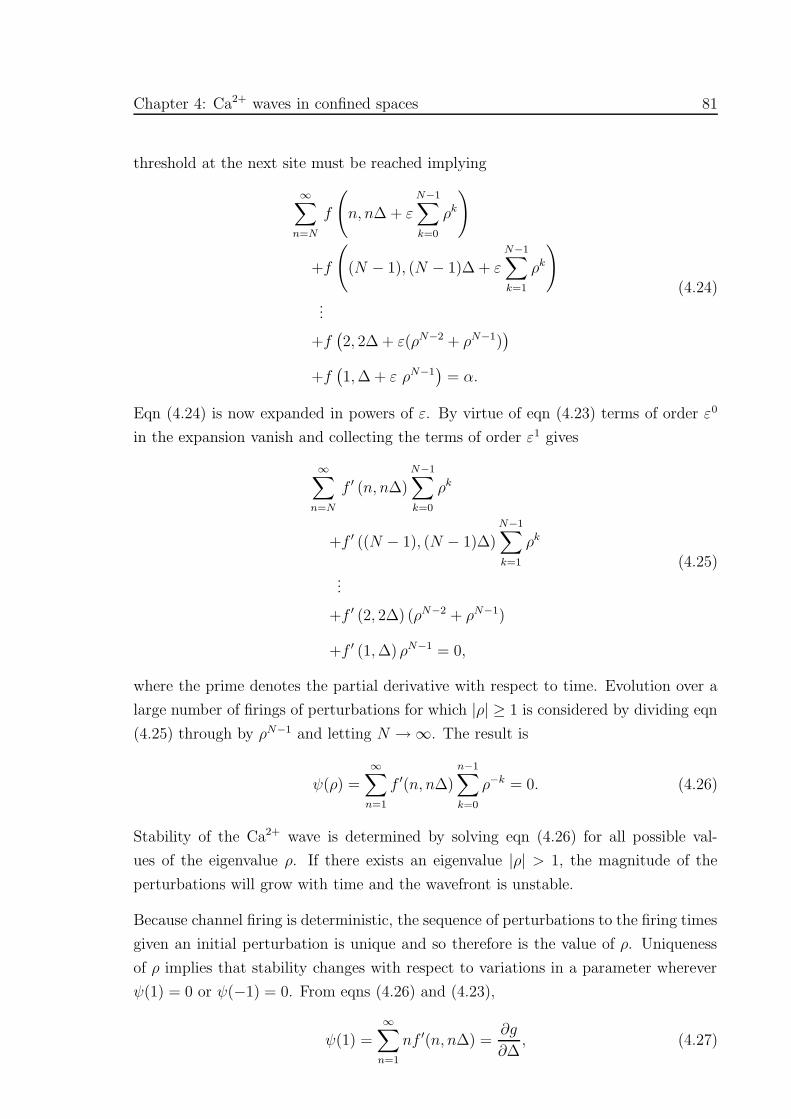
Chapter 4: Ca2+ waves in confined spaces 81
threshold at the next site must be reached implying
∞∑
n=N
f
(n, n∆ + ε
N−1∑
k=0
ρk
)
+f
((N − 1), (N − 1)∆ + ε
N−1∑
k=1
ρk
)
...
+f(2, 2∆ + ε(ρN−2 + ρN−1)
)
+f(1,∆ + ε ρN−1
)= α.
(4.24)
Eqn (4.24) is now expanded in powers of ε. By virtue of eqn (4.23) terms of order ε0
in the expansion vanish and collecting the terms of order ε1 gives
∞∑
n=N
f ′ (n, n∆)
N−1∑
k=0
ρk
+f ′ ((N − 1), (N − 1)∆)N−1∑
k=1
ρk
...
+f ′ (2, 2∆) (ρN−2 + ρN−1)
+f ′ (1,∆) ρN−1 = 0,
(4.25)
where the prime denotes the partial derivative with respect to time. Evolution over a
large number of firings of perturbations for which |ρ| ≥ 1 is considered by dividing eqn
(4.25) through by ρN−1 and letting N → ∞. The result is
ψ(ρ) =∞∑
n=1
f ′(n, n∆)n−1∑
k=0
ρ−k = 0. (4.26)
Stability of the Ca2+ wave is determined by solving eqn (4.26) for all possible val-
ues of the eigenvalue ρ. If there exists an eigenvalue |ρ| > 1, the magnitude of the
perturbations will grow with time and the wavefront is unstable.
Because channel firing is deterministic, the sequence of perturbations to the firing times
given an initial perturbation is unique and so therefore is the value of ρ. Uniqueness
of ρ implies that stability changes with respect to variations in a parameter wherever
ψ(1) = 0 or ψ(−1) = 0. From eqns (4.26) and (4.23),
ψ(1) =∞∑
n=1
nf ′(n, n∆) =∂g
∂∆, (4.27)

Chapter 4: Ca2+ waves in confined spaces 82
therefore stability changes at the stationary points of g(∆). Also from eqn (4.26),
ψ(−1) =
∞∑
n=1
1
2(1 − (−1)n) f ′(n, n∆). (4.28)
The explicit formula for f ′ is given by
f ′(n, n∆) =
∞∑
k=0
∞∑
m=0
[G(n, n∆, λ) − Θ(n∆ − τ)G(n, n∆ − τ, λ)]Y (0, λm)Z(0, λk),
(4.29)
for n∆ 6= τ , where λ = λ2m + λ2
k and the function G, defined by
G(x, t, λ) =∂I
∂t=e−x
2
4t− λt
√4πt
, (4.30)
is obtained by differentiating eqn (G.31) of Appendix G. In eqn (4.29), the Y, Z, λm
and λk are defined by eqns (4.15)-(4.19).
The ranges of values of ∆ over which the Ca2+ wavefront is stable or unstable are
completely determined by the roots of eqns (4.27) and (4.28). As the value of ∆ is
varied, the stability of the Ca2+ wave solutions alternate between stable and unstable
as it passes through each of these solutions.
4.3 Results
Results are now given of the analysis of the existence and stability of FDF Ca2+ wave-
fronts and the simulation of their evolution, using the formulae given in the previous
section and 4.2.2. Further details of the numerical techniques used here are given in
Appendix F. Values of variables and parameters are given in the non-dimensional form
defined in (4.7).
Firstly, results are given for a channel opening time of τ = 0.05 and for the absence of
Ca2+ pumps, that is, for SR and SL pump rates of γsr = γsl = 0 respectively. Results
for the existence and stability of Ca2+ waves are given in the form of curves of the
function g with respect to the firing interval ∆, obtained by evaluating eqn (4.23) with
all other parameters held constant. By eqn (4.23) the ordinate of these curves is the
value of α required for Ca2+ waves for a given value of ∆.
Fig. 4.2 shows the effects of lateral obstructions on the propagation of Ca2+ waves.
Variations in the values of the channel parameter, α, with respect to values of ∆ are
shown for different values of the non-dimensional domain width, w = 0.1, 1 and 100
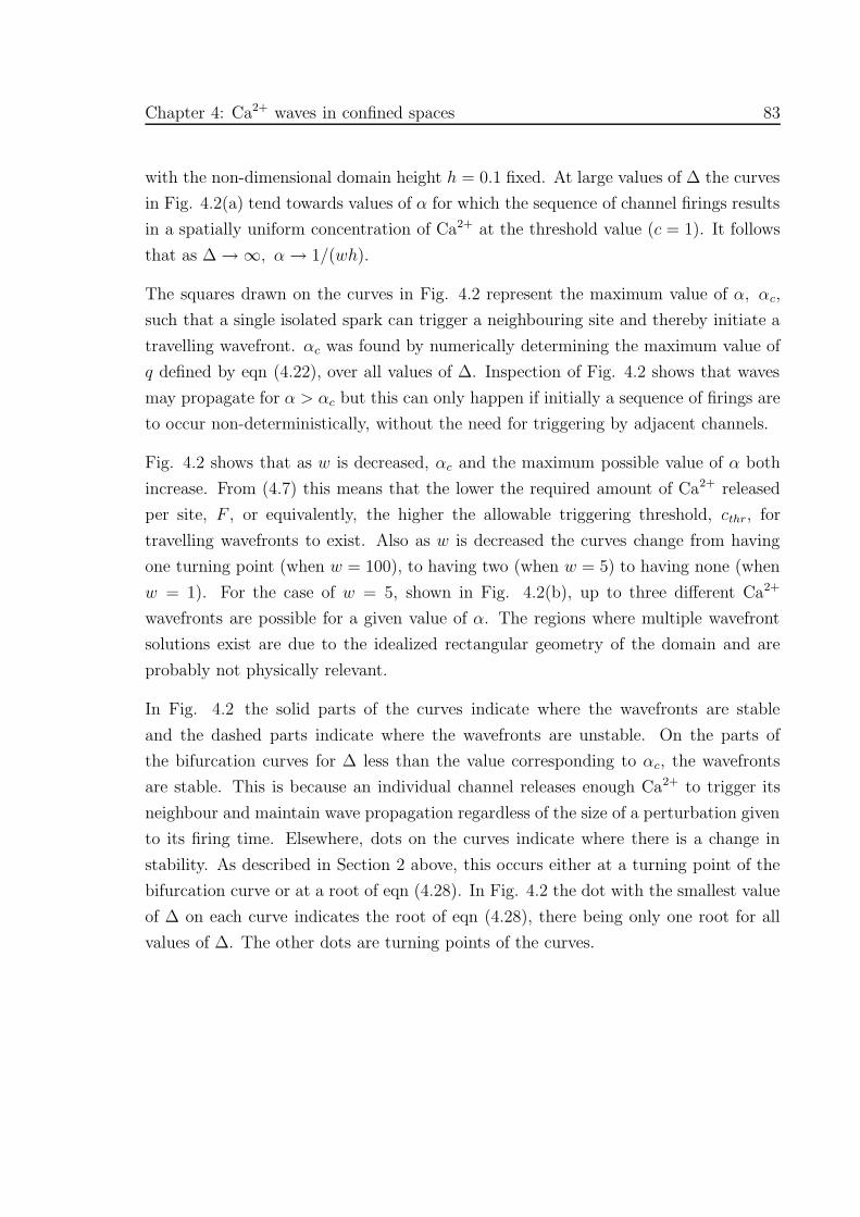
Chapter 4: Ca2+ waves in confined spaces 83
with the non-dimensional domain height h = 0.1 fixed. At large values of ∆ the curves
in Fig. 4.2(a) tend towards values of α for which the sequence of channel firings results
in a spatially uniform concentration of Ca2+ at the threshold value (c = 1). It follows
that as ∆ → ∞, α → 1/(wh).
The squares drawn on the curves in Fig. 4.2 represent the maximum value of α, αc,
such that a single isolated spark can trigger a neighbouring site and thereby initiate a
travelling wavefront. αc was found by numerically determining the maximum value of
q defined by eqn (4.22), over all values of ∆. Inspection of Fig. 4.2 shows that waves
may propagate for α > αc but this can only happen if initially a sequence of firings are
to occur non-deterministically, without the need for triggering by adjacent channels.
Fig. 4.2 shows that as w is decreased, αc and the maximum possible value of α both
increase. From (4.7) this means that the lower the required amount of Ca2+ released
per site, F , or equivalently, the higher the allowable triggering threshold, cthr, for
travelling wavefronts to exist. Also as w is decreased the curves change from having
one turning point (when w = 100), to having two (when w = 5) to having none (when
w = 1). For the case of w = 5, shown in Fig. 4.2(b), up to three different Ca2+
wavefronts are possible for a given value of α. The regions where multiple wavefront
solutions exist are due to the idealized rectangular geometry of the domain and are
probably not physically relevant.
In Fig. 4.2 the solid parts of the curves indicate where the wavefronts are stable
and the dashed parts indicate where the wavefronts are unstable. On the parts of
the bifurcation curves for ∆ less than the value corresponding to αc, the wavefronts
are stable. This is because an individual channel releases enough Ca2+ to trigger its
neighbour and maintain wave propagation regardless of the size of a perturbation given
to its firing time. Elsewhere, dots on the curves indicate where there is a change in
stability. As described in Section 2 above, this occurs either at a turning point of the
bifurcation curve or at a root of eqn (4.28). In Fig. 4.2 the dot with the smallest value
of ∆ on each curve indicates the root of eqn (4.28), there being only one root for all
values of ∆. The other dots are turning points of the curves.
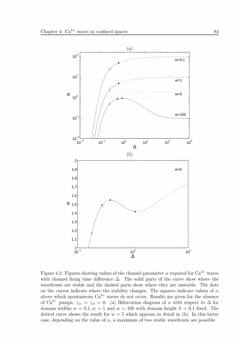
Chapter 4: Ca2+ waves in confined spaces 84
(a)
10−2
10−1
100
101
102
103
10−2
10−1
100
101
102
∆
α
w=100
w=5
w=1
w=0.1
(b)
10−1
100
101
1
1.1
1.2
1.3
1.4
1.5
1.6
1.7
1.8
1.9
2
∆
α
w=5
Figure 4.2: Figures showing values of the channel parameter α required for Ca2+ waveswith channel firing time difference ∆. The solid parts of the curve show where thewavefronts are stable and the dashed parts show where they are unstable. The dotson the curves indicate where the stability changes. The squares indicate values of αabove which spontaneous Ca2+ waves do not occur. Results are given for the absenceof Ca2+ pumps, γsr = γsl = 0. (a) Bifurcation diagram of α with respect to ∆ fordomain widths w = 0.1, w = 1 and w = 100 with domain height h = 0.1 fixed. Thedotted curve shows the result for w = 5 which appears in detail in (b). In this lattercase, depending on the value of α, a maximum of two stable wavefronts are possible.
Chapter 4: Ca2+ waves in confined spaces 85
10−2
10−1
100
101
102
103
10−2
10−1
100
101
102
∆
α
h=0.01
h=0.1
h=1
Figure 4.3: Bifurcation diagrams of α with respect to ∆ for domain heights h =0.01, h = 0.1 and h = 1 with domain width w = 10 fixed. Results are given for theabsence of Ca2+ pumps, γsr = γsl = 0.

Chapter 4: Ca2+ waves in confined spaces 86
10−2
10−1
100
0
5
10
15
20
25
30
h
Wav
e sp
eed
Wave speedα
cγsr
=0γsr
=0.5
10−2
10−1
1000
5
10
15
αc
10−2
10−1
1000
5
10
15
10−2
10−1
1000
5
10
15
10−2
10−1
1000
5
10
15
Figure 4.4: Figure showing the variations in wave speed and channel parameter criticalvalue, αc, with domain height, h, for the parameter values α = 0.25, w = 10 andγsl = 0. Results for two different values of the SR pump rate are given, γsr = 0(circles) and γsr = 0.5 (crosses).
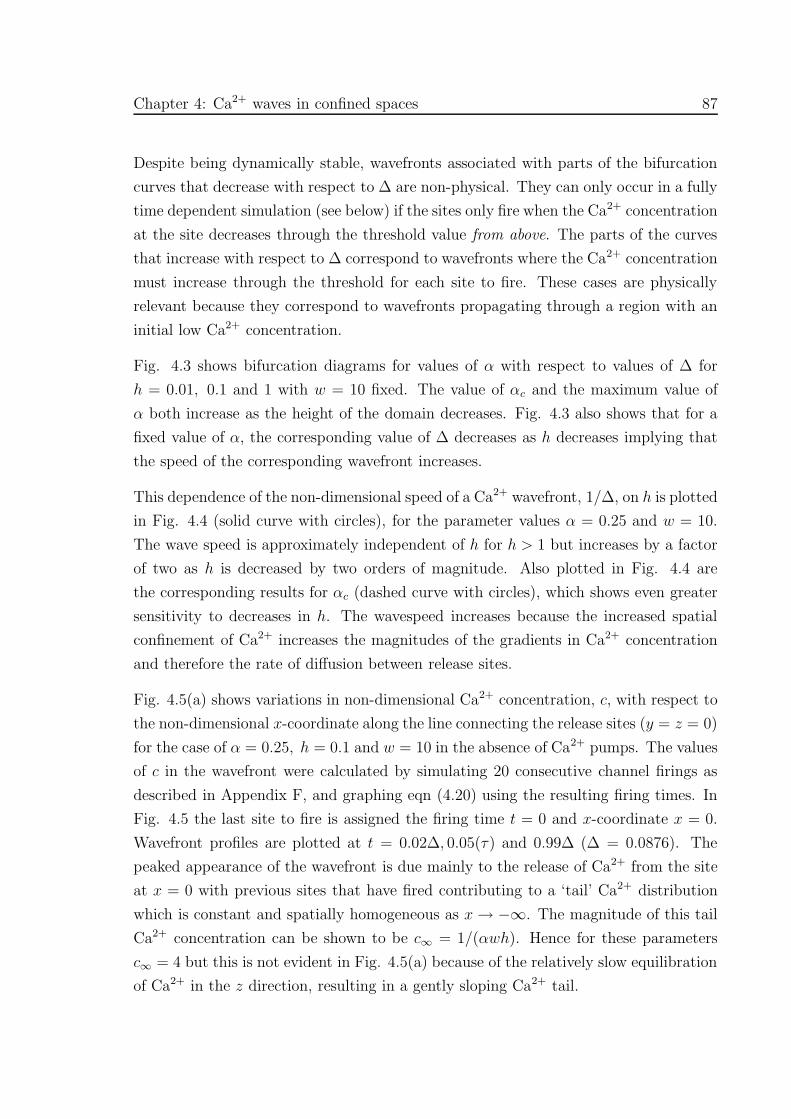
Chapter 4: Ca2+ waves in confined spaces 87
Despite being dynamically stable, wavefronts associated with parts of the bifurcation
curves that decrease with respect to ∆ are non-physical. They can only occur in a fully
time dependent simulation (see below) if the sites only fire when the Ca2+ concentration
at the site decreases through the threshold value from above. The parts of the curves
that increase with respect to ∆ correspond to wavefronts where the Ca2+ concentration
must increase through the threshold for each site to fire. These cases are physically
relevant because they correspond to wavefronts propagating through a region with an
initial low Ca2+ concentration.
Fig. 4.3 shows bifurcation diagrams for values of α with respect to values of ∆ for
h = 0.01, 0.1 and 1 with w = 10 fixed. The value of αc and the maximum value of
α both increase as the height of the domain decreases. Fig. 4.3 also shows that for a
fixed value of α, the corresponding value of ∆ decreases as h decreases implying that
the speed of the corresponding wavefront increases.
This dependence of the non-dimensional speed of a Ca2+ wavefront, 1/∆, on h is plotted
in Fig. 4.4 (solid curve with circles), for the parameter values α = 0.25 and w = 10.
The wave speed is approximately independent of h for h > 1 but increases by a factor
of two as h is decreased by two orders of magnitude. Also plotted in Fig. 4.4 are
the corresponding results for αc (dashed curve with circles), which shows even greater
sensitivity to decreases in h. The wavespeed increases because the increased spatial
confinement of Ca2+ increases the magnitudes of the gradients in Ca2+ concentration
and therefore the rate of diffusion between release sites.
Fig. 4.5(a) shows variations in non-dimensional Ca2+ concentration, c, with respect to
the non-dimensional x-coordinate along the line connecting the release sites (y = z = 0)
for the case of α = 0.25, h = 0.1 and w = 10 in the absence of Ca2+ pumps. The values
of c in the wavefront were calculated by simulating 20 consecutive channel firings as
described in Appendix F, and graphing eqn (4.20) using the resulting firing times. In
Fig. 4.5 the last site to fire is assigned the firing time t = 0 and x-coordinate x = 0.
Wavefront profiles are plotted at t = 0.02∆, 0.05(τ) and 0.99∆ (∆ = 0.0876). The
peaked appearance of the wavefront is due mainly to the release of Ca2+ from the site
at x = 0 with previous sites that have fired contributing to a ‘tail’ Ca2+ distribution
which is constant and spatially homogeneous as x → −∞. The magnitude of this tail
Ca2+ concentration can be shown to be c∞ = 1/(αwh). Hence for these parameters
c∞ = 4 but this is not evident in Fig. 4.5(a) because of the relatively slow equilibration
of Ca2+ in the z direction, resulting in a gently sloping Ca2+ tail.
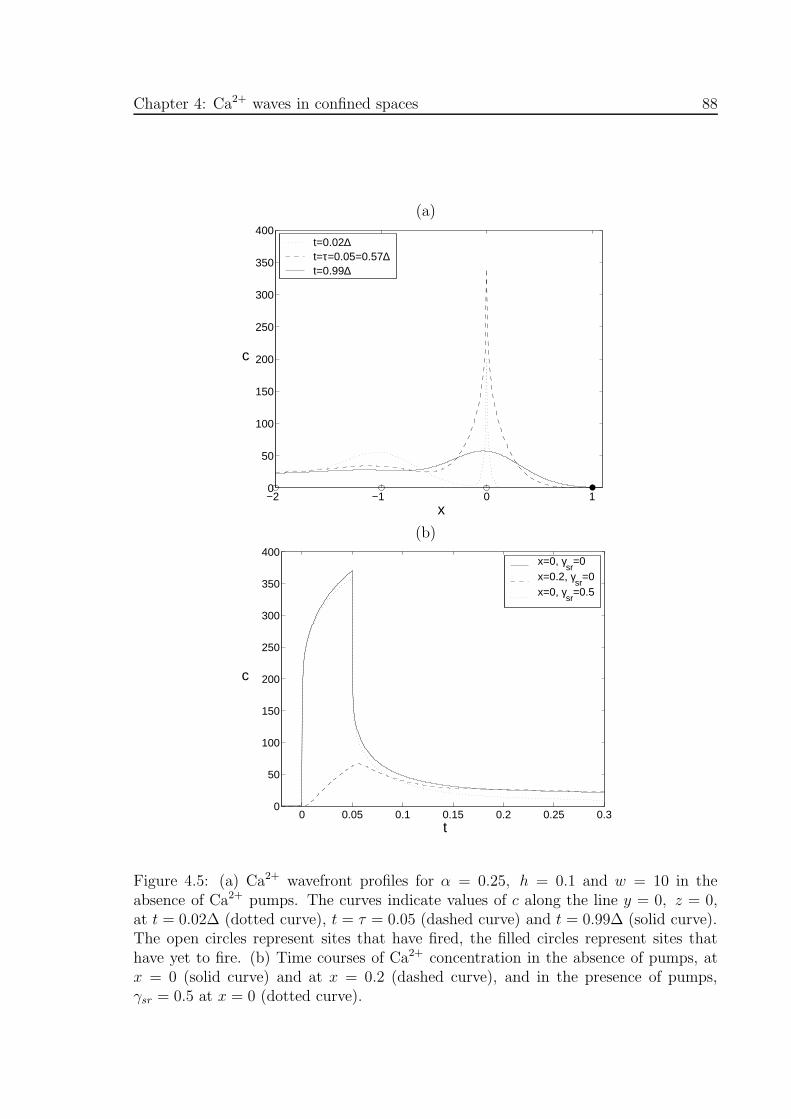
Chapter 4: Ca2+ waves in confined spaces 88
(a)
−2 −1 0 10
50
100
150
200
250
300
350
400
x
c
t=0.02∆ t=τ=0.05=0.57∆ t=0.99∆
(b)
0 0.05 0.1 0.15 0.2 0.25 0.30
50
100
150
200
250
300
350
400
t
c
x=0, γsr
=0 x=0.2, γ
sr=0
x=0, γsr
=0.5
Figure 4.5: (a) Ca2+ wavefront profiles for α = 0.25, h = 0.1 and w = 10 in theabsence of Ca2+ pumps. The curves indicate values of c along the line y = 0, z = 0,at t = 0.02∆ (dotted curve), t = τ = 0.05 (dashed curve) and t = 0.99∆ (solid curve).The open circles represent sites that have fired, the filled circles represent sites thathave yet to fire. (b) Time courses of Ca2+ concentration in the absence of pumps, atx = 0 (solid curve) and at x = 0.2 (dashed curve), and in the presence of pumps,γsr = 0.5 at x = 0 (dotted curve).
Chapter 4: Ca2+ waves in confined spaces 89
−3−2
−10
12 −3
−2−1
01
23
0
5
10
15
20
25
30
35
z x
c
Figure 4.6: Ca2+ concentration, c, with respect to x and z at t = 0.99∆ on the planey = 0 in the presence of SR Ca2+ pumps, γsr = 0.5 and γsl = 0. The dashed lines markthe positions of the sites that have fired, the solid lines mark the positions of sites thatare yet to fire.
Chapter 4: Ca2+ waves in confined spaces 90
Time courses of Ca2+ corresponding to the wavefront in Fig. 4.5(a) are shown in Fig.
4.5(b). Results are given for c with respect to non-dimensional time, t, at x = 0 (solid
curve) and x = 0.2 (dashed curve). Note that the peak value of c at x = 0 is reached
at t = τ and that the peak value of c measured just off the release site, at x = 0.2,
is significantly less. The Ca2+ time course for a wavefront with the same parameters
except with a SR pump rate of γsr = 0.5 is also shown in Fig. 4.5(b) (dotted curve).
There is a slight decrease in the peak value of c relative to the case of γsr = 0, but
the most significant effect is in the Ca2+ tail. The presence of pumps removes all Ca2+
from the domain so that c → 0 as t → ∞ in the time courses and c → 0 as x → −∞in the wavefronts.
Fig. 4.6 depicts the wavefront at t = 0.99∆ (∆ = 0.1) in the presence of SR pumps,
γsr = 0.5, γsl = 0, in both the x and z directions. Due to the small value of h used,
c is approximately constant with respect to y for these parameters. The presence of
pumps has reduced the peak value of c to 32.5 in this figure from 57.4 in Fig. 4.5(a)
(see curve for t = 0.99∆).
Now the corresponding results for the existence and stability of FDF Ca2+ waves in
the presence of SR and SL pumps (γsr ≥ 0, γsl ≥ 0) will be given. The effects of SR
Ca2+ pumps only, γsr > 0 and γsl = 0, on the bifurcation diagrams for h = 0.1 and
w = 10 are shown in Fig. 4.7. Results for four different SR pump rates, γsr = 0 (dotted
curve), 5 × 10⁻⁶, 0.5 and 5, are given (the result for γsr = 0 also appears in Fig. 4.3).
For γsr = 5× 10⁻⁶ an additional turning point now appears and α→ 0 as ∆ → ∞. A
change of stability occurs at this new turning point leading to stable (but non-physical)
wavefronts for points on the decreasing part of the curve above the turning point. As
γsr is increased to 0.5 the upper two turning points on the previous curve disappear
along with the region of instability between them. Also, the lower region of instability
shrinks but never completely disappears as γsr is increased further.
As γsr is increased to 5, the last site that fires becomes the main contributor towards
Ca2+ in the wavefront, with Ca2+ released from previous sites being removed more
rapidly by the higher pump rate. As discussed above, regions of the curves for α > αc
depend on the contribution of several channels, so these regions will shrink as γsr
increases. As seen in Fig. 4.7, αc tends towards the peak value of α, which also
decreases as γsr increases. Note also in Fig. 4.7, the increase in values of ∆ on the
increasing parts of the curves as γsr is increased, indicating a slowing of the wavefront
in the presence of pumps.
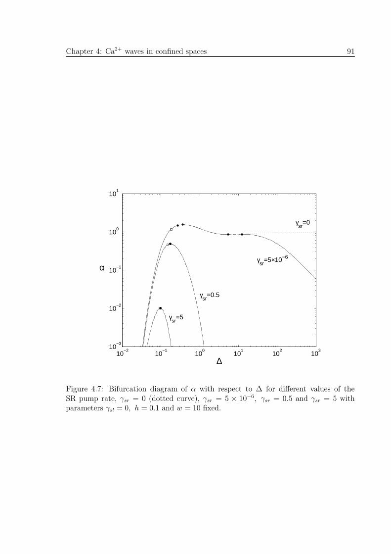
Chapter 4: Ca2+ waves in confined spaces 91
10−2
10−1
100
101
102
103
10−3
10−2
10−1
100
101
∆
α
γsr
=0
γsr
=5×10⁻⁶
γsr
=0.5
γsr
=5
Figure 4.7: Bifurcation diagram of α with respect to ∆ for different values of theSR pump rate, γsr = 0 (dotted curve), γsr = 5 × 10⁻⁶, γsr = 0.5 and γsr = 5 withparameters γsl = 0, h = 0.1 and w = 10 fixed.
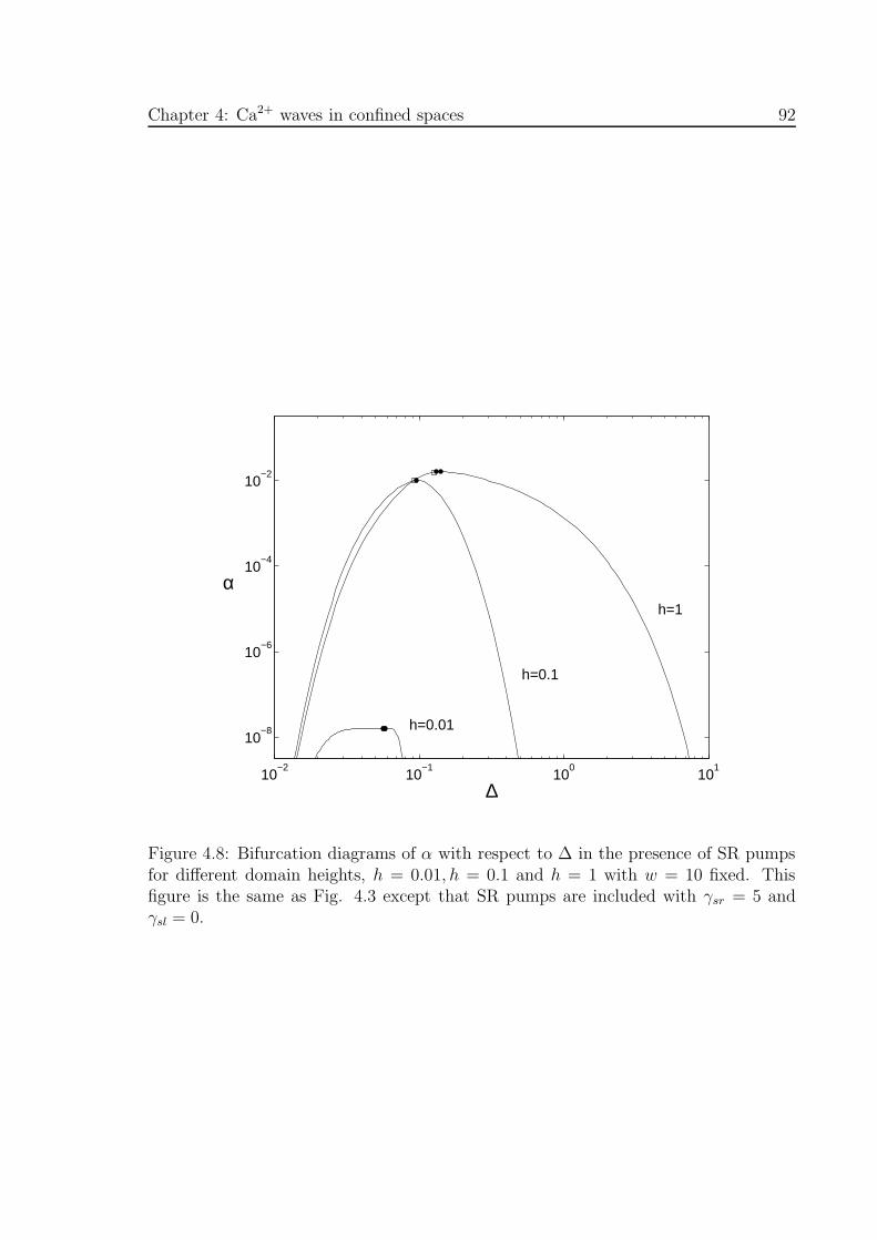
Chapter 4: Ca2+ waves in confined spaces 92
10−2
10−1
100
101
10−8
10−6
10−4
10−2
∆
α h=1
h=0.1
h=0.01
Figure 4.8: Bifurcation diagrams of α with respect to ∆ in the presence of SR pumpsfor different domain heights, h = 0.01, h = 0.1 and h = 1 with w = 10 fixed. Thisfigure is the same as Fig. 4.3 except that SR pumps are included with γsr = 5 andγsl = 0.
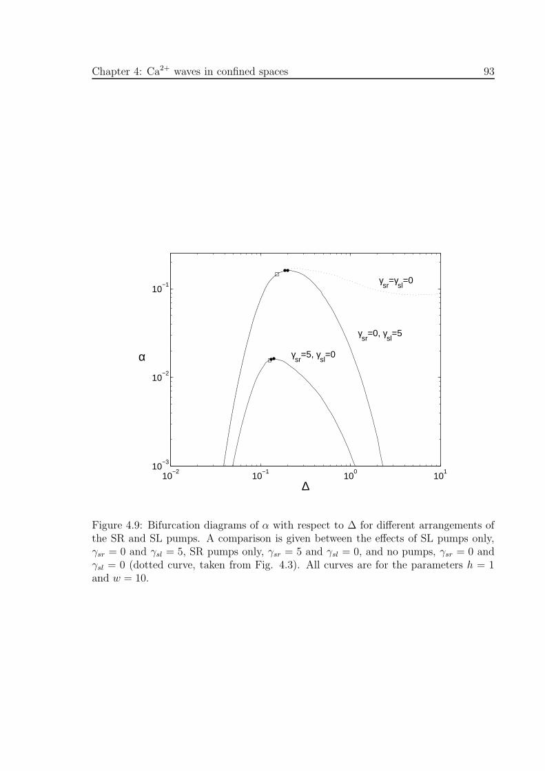
Chapter 4: Ca2+ waves in confined spaces 93
10−2
10−1
100
101
10−3
10−2
10−1
∆
α
γsr
=γsl
=0
γsr
=0, γsl
=5
γsr
=5, γsl
=0
Figure 4.9: Bifurcation diagrams of α with respect to ∆ for different arrangements ofthe SR and SL pumps. A comparison is given between the effects of SL pumps only,γsr = 0 and γsl = 5, SR pumps only, γsr = 5 and γsl = 0, and no pumps, γsr = 0 andγsl = 0 (dotted curve, taken from Fig. 4.3). All curves are for the parameters h = 1and w = 10.

Chapter 4: Ca2+ waves in confined spaces 94
Fig. 4.8 shows the effects on the bifurcation diagrams of keeping the SR pump rate
constant and varying h with w = 10 fixed. Results for h = 0.01, 0.1 and 1 are shown
with γsr = 5 and γsl = 0. Note that the effects of the pumps become more pronounced
as h is decreased. For example, the peak value of α for each curve decreases as h
is increased whereas the converse is true when γsr = 0 (see Fig. 4.3). This occurs
because even though a fixed amount of Ca2+ is released by each spark, independent of
the dimensions of the domain, the rate at which the pumps remove this Ca2+ increases
as h decreases.
This effect is also illustrated in Fig. 4.4 where the wave speed and αc are plotted with
respect to h for a wavefront with the parameters α = 0.25, w = 10, γsr = 0.5 and
γsl = 0. The slowing of the wavefront in the presence of pumps is evident (solid curve
with crosses) but far more striking is the effect of pumps on αc (dashed curve with
crosses). As h is decreased from 1, the wave speed and αc both increase, peak and then
decrease. This shows that enhancement of propagation of Ca2+ waves due to increased
spatial confinement of Ca2+ release is counteracted by the increased effect of the Ca2+
pumps. The curve of wave speed with respect to h terminates when h is sufficiently
small that travelling wavefront solutions no longer exist.
Fig. 4.9 shows a comparison between the effects of SR and SL pumps. Bifurcation
curves are given for SL pumps only, γsr = 0 and γsl = 5, for h = 1 as well as the
corresponding results for SR pumps only, γsr = 5 and γsl = 0 (taken from Fig. 4.8).
Also, the corresponding results in the absence of pumps are given (dotted curve, taken
from Fig. 4.3). The arrangement of pumps is more significant the larger the value of
h. For the case where there are only SL pumps, the larger the value of h the greater
the distance over which Ca2+ must diffuse to reach the pumps relative to the distance
to the next site. The effect of the pumps on wave propagation is therefore less and
the bifurcation curve more closely resembles that in the absence of Ca2+ pumps. For
small h, where the distribution of Ca2+ in the y direction can be considered uniform,
SR and SL pumps with the same pump rate are equivalent and the bifurcation curves
for the two different arrangements of pumps described above will be the same.
Fig. 4.10(a) shows bifurcation diagrams of α with respect to ∆ for different values of
the channel opening time, τ = 1×10⁻⁴, 0.05 (dotted curve, also appearing in Fig. 4.3)
and 1. The parameters h = 0.1, w = 10 and γsr = γsl = 0 are all held constant. Since
τ = 1 × 10⁻⁴ is much less than the values of ∆ in the range given in the figure, the
curve for this value of τ closely approximates the bifurcation curve where the release
of Ca2+ is an impulse. The main effect of increasing τ is to decrease the wave speed
which occurs because the distributed release of Ca2+ from a site decreases the rate of

Chapter 4: Ca2+ waves in confined spaces 95
diffusion of Ca2+ to the next site. When ∆ < τ , the release of Ca2+ from two or more
sites overlap however the stability analysis, as indicated in Fig. 4.10(a), shows that
Ca2+ waves are stable even when there are an arbitrarily large number of overlapping
firings (∆ << τ). The wavefronts for such a case are illustrated in Fig. 4.10(b) for
α = 0.01 and τ = 1. c is plotted with respect to x at t = 0.99∆ along the line
y = z = 0 for the parameter values γsr = 0 (solid curve) and γsr = 2 (dashed curve)
with the same values of h, w and γsl as for Fig. 4.10(a). The firing time differences
for these wavefronts are ∆ = 0.0820 and ∆ = 0.2186 for the two different values of γsr
implying that respectively 12 and 4 channels are open simultaneously in the wavefront.
In the absence of pumps, Ca2+ released from the open channels accumulates leading to
a wavefront with a rising tail. When γsr = 2, however, the rate of release of Ca2+ from
the open channels is balanced by its rate of removal by the pumps thereby leading to
a series of peaks of the same height in the wavefront.

Chapter 4: Ca2+ waves in confined spaces 96
(a)
10−2
10−1
100
101
102
103
10−2
10−1
100
∆
α
τ=1× 10⁻⁴
τ=0.05
τ=1
(b)
−3 −2 −1 0 10
100
200
300
400
500
600
700
x
c
γsr
=0γsr
=2
Figure 4.10: (a) Bifurcation diagrams of α with respect to ∆ for different values ofthe channel opening time τ = 1 × 10⁻⁴, 0.05 and 1. Curves are given for the absenceof Ca2+ pumps, γsr = γsl = 0, and for the parameters h = 0.1 and w = 10. (b)Corresponding wavefront profiles at t = 0.99∆ for the case of τ = 1 and α = 0.01. Thesolid curve is for γsr = 0, the dashed curve is for γsr = 2. The parameters w, h and γsl
are the same as for (a).
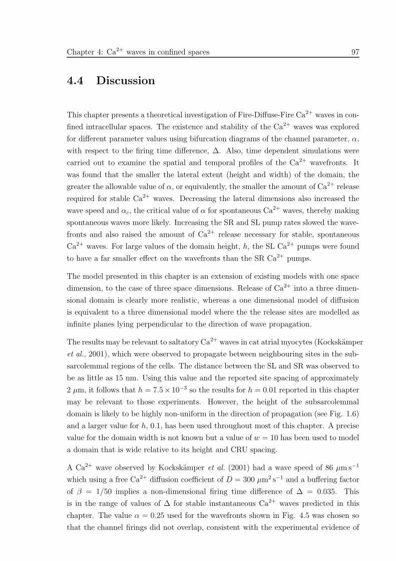
Chapter 4: Ca2+ waves in confined spaces 97
4.4 Discussion
This chapter presents a theoretical investigation of Fire-Diffuse-Fire Ca2+ waves in con-
fined intracellular spaces. The existence and stability of the Ca2+ waves was explored
for different parameter values using bifurcation diagrams of the channel parameter, α,
with respect to the firing time difference, ∆. Also, time dependent simulations were
carried out to examine the spatial and temporal profiles of the Ca2+ wavefronts. It
was found that the smaller the lateral extent (height and width) of the domain, the
greater the allowable value of α, or equivalently, the smaller the amount of Ca2+ release
required for stable Ca2+ waves. Decreasing the lateral dimensions also increased the
wave speed and αc, the critical value of α for spontaneous Ca2+ waves, thereby making
spontaneous waves more likely. Increasing the SR and SL pump rates slowed the wave-
fronts and also raised the amount of Ca2+ release necessary for stable, spontaneous
Ca2+ waves. For large values of the domain height, h, the SL Ca2+ pumps were found
to have a far smaller effect on the wavefronts than the SR Ca2+ pumps.
The model presented in this chapter is an extension of existing models with one space
dimension, to the case of three space dimensions. Release of Ca2+ into a three dimen-
sional domain is clearly more realistic, whereas a one dimensional model of diffusion
is equivalent to a three dimensional model where the the release sites are modelled as
infinite planes lying perpendicular to the direction of wave propagation.
The results may be relevant to saltatory Ca2+ waves in cat atrial myocytes (Kockskamper
et al., 2001), which were observed to propagate between neighbouring sites in the sub-
sarcolemmal regions of the cells. The distance between the SL and SR was observed to
be as little as 15 nm. Using this value and the reported site spacing of approximately
2 µm, it follows that h = 7.5× 10⁻³ so the results for h = 0.01 reported in this chapter
may be relevant to those experiments. However, the height of the subsarcolemmal
domain is likely to be highly non-uniform in the direction of propagation (see Fig. 1.6)
and a larger value for h, 0.1, has been used throughout most of this chapter. A precise
value for the domain width is not known but a value of w = 10 has been used to model
a domain that is wide relative to its height and CRU spacing.
A Ca2+ wave observed by Kockskamper et al. (2001) had a wave speed of 86 µm s−1
which using a free Ca2+ diffusion coefficient of D = 300 µm2 s−1 and a buffering factor
of β = 1/50 implies a non-dimensional firing time difference of ∆ = 0.035. This
is in the range of values of ∆ for stable instantaneous Ca2+ waves predicted in this
chapter. The value α = 0.25 used for the wavefronts shown in Fig. 4.5 was chosen so
that the channel firings did not overlap, consistent with the experimental evidence of
Chapter 4: Ca2+ waves in confined spaces 98
Kockskamper et al. (2001). However, channel parameters obtained from theoretical
studies of sparks in cardiac cells typically result in far lower values of α. For example,
in a theoretical study of the release of Ca2+ from the SR in the dyadic cleft of cardiac
cells (Langer and Peskoff, 1996), a channel current, I, of 2 pA is used with a channel
firing time of Ton = 20 ms. This gives a release flux of F =ITon
2C= 2 × 10⁻¹⁹ mol,
where C = 9.65 × 10⁴ is the Faraday constant, and using a firing threshold of cthr = 1
µM this implies α =cthrd
3
βF= 2 × 10⁻³. This value is well below αc for most of the
parameter values used in this study. It is an open question whether or not α exceeding
the critical value, αc, is a significant effect in reality. However the combination of high
pump rates and small domain heights could cause propagation failure. Such would be
the case for the parameters h = 0.01 and γsr = 5 for α = 2 × 10⁻³ (see Fig. 4.8).
Note that the value of Ton = 20 ms corresponds to a value of τ =βDTon
d2= 0.03 which
is close to the value of τ = 0.05 used in this chapter.
A realistic value for γ is obtained from Fig. 7 of Kockskamper et al. (2001) which shows
a Ca2+ concentration decay half-time of approximately T1/2 = 200 ms, giving a decay
constant of kdec = ln 2/T1/2 = 3.5. Assuming that this decay is completely due to the
SR pumps and that the tail Ca2+ is homogeneous with respect to space in the domain,
it can be shown that for h << w, kdec =ksr
2h. It follows that γsr =
d2hkdec
βD= 0.4, close
to the value of γsr = 0.5 used in this chapter. In the time course of Ca2+ shown in Fig.
4.5(b) for γsr = 0.5 at x = 0 (dotted curve), pumps contribute significantly to the the
decay of Ca2+ for values of t greater than approximately 0.15 . For 0.05 < t < 0.15
there is a more rapid phase of Ca2+ decay dominated by diffusion away from the release
site.
Using the firing threshold of cthr = 1 µM gives a peak Ca2+ concentration at the release
site in the hundreds of µM range (see Figs. 4.5 and 4.10(b)). These predictions are
consistent with those from theoretical studies of Ca2+ release into the dyadic cleft of
cardiac cells (Peskoff et al., 1992 and Langer and Peskoff, 1996).
The comparison of the results reported here with those of Kockskamper et al. (2001) is
complicated since in reality the dimensions of the subsarcolemmal domain is likely to be
highly non-uniform. Further, Ca2+ release into the subsarcolemmal region is likely not
to be completely confined by the SR as in the present model, but also simultaneously
diffuse into the central parts of the cell. An alternative approach to the modelling
is to not use an impermeable SR, but make transverse diffusion of Ca2+ slower than
longitudinal diffusion in the peripheral region (Subramanian et al., 2001).

Chapter 4: Ca2+ waves in confined spaces 99
A peripherally located ER/SR is a significant feature of several different cell types
including the rat megarkaryocyte (Thomas et al., 2001), rabbit heart Purkinje cell
(Cordeiro et al., 2001) and smooth muscle (Kargacin and Fay, 1991). The arrangement
of surface and internal membranes may play a role in the formation and propagation
of Ca2+ waves in these cells. Indeed, in the case of the rat megarkaryocyte (Thomas et
al., 2001), Xenopis laevis egg (Fontanilla and Nuccitelli, 1998) and vascular endothelial
cell (Huser and Blatter, 1997), the higher wave speed observed in the peripheral region
of the cell relative to the central part could be due to higher spatial confinement of
Ca2+ release in the former, consistent with the results reported in this thesis.
¨
100
Appendices
Appendix A
Detailed mathematical model of the G protein cas-
cade
In this section, a detailed mathematical model is formulated for the G protein cascade
occurring due to a homogeneous distribution of P2Y2 receptors in the cell membrane.
By making various assumptions, a reduced and simplified set of model equations are
then derived. The detailed schematic diagram for the G protein cascade is shown in
Fig. 2.2.
P2Y2 receptor model
The following process by which any G protein coupled receptor activates G protein
molecules is well established, see for example Lamb and Pugh (1992), Lauffenburger
and Linderman (pp 185-187, 1993). A P2Y2 receptor binds a molecule of G · GDP
from the membrane and brings about the exchange of a GTP nucleotide (assumed to
be immediately available from the cytosol) for the GDP nucleotide bound to the G
protein. These processes can be modelled with the scheme
k+1 k2 k−1
G · GDP + P2Y2 � P2Y2·G · GDP → P2Y2 · G · GTP � P2Y2 + G · GTP,k−1 k+
1
for forward and reverse rate constants k+1 , k
−1 . In Appendix B it is shown that
k2 = k2 + (k∗2 − k2)ρr,
where k∗2, k2 are the exchange rates for the ligand bound and unbound receptor. ρr is
the ratio of the amount of ligand bound receptor to total receptor and is determined

Appendices 101
independently of the G protein kinetics.
G protein subunit kinetics
The kinetics for the interaction of the G protein subunits and the trimer is assumed to
depend on whether the nucleotide bound to it is GTP or GDP. Hence
k−3G · GTP � Gα · GTP + Gβγ
k+3
and
k−3Gα · GDP + Gβγ � G · GDP,
k+3
for forward rate constants k+3 , k
+3 and reverse rate constants k−3 , k
−3 .
PLC effector model
The activity of the PLC molecule is mediated by several different binding sites (Rebbec-
chi and Pentyala, 2000). Of relevance to the present study are the three sites each of
which bind to the Gα subunit, Ca2+ ion and PIP2 molecule. It is assumed that the
probability of binding to any of these sites is not dependent on the state of occupancy
of the other sites.
Binding of the Gα subunit
The Gα · GTP (Gαq/11· GTP) molecules are deactivated by binding to GTPase acti-
vating proteins (GAPs; see Iyengar, 1997). PLC-β1 (hereafter PLC) itself acts as a
GAP for Gq (Morris and Scarlata, 1997; Mukhophadhyay and Ross, 1999) hence the
interaction of the G-protein with PLC is modelled with the following kinetics,
k+1 k2
Gα · GTP + PLC � Gα · GTP · PLC →k−1
k−1Gα · GDP · PLC � Gα · GDP + PLC,
k+1

Appendices 102
for forward rate constants k+1 , k2 and reverse rate constant k−1 .
Binding of Ca2+
The kinetics for the binding of Ca2+ from the cytosol to PLC are
k+3
PLC + Ca2+� PLC · Ca2+ .k−3
Binding of PIP2
PLC binds to the membrane at the pleckstrin homology domain of PIP2 · PLC which
is also bound to Ca2+ and Gα · GTP is considered to be most effective in hydrolysing
PIP2 molecules to give IP3 and diacylglycerol. The kinetics for the interaction of PLC
and PIP2 are
k+4 kh
PLC + PIP2 � PLC · PIP2 → IP3 + PLC,k−4
for forward and reverse rate constants k+4 , k
−4 . In a similar calculation to that in
Appendix B it can be shown that
kh = kh + (k∗h − kh)ρb, (A.1)
with ρb being the ratio of the amount of Ca2+ and Gα ·GTP bound PLC to total PLC.
Mathematical formulation
Using the law of mass action, the kinetic schemes presented above can be formulated
in terms of a set of coupled ordinary differential equations. It suffices to give these
equations in the shorthand form
du
dt= Au + Buu, (A.2)
u = u0 at t = 0, (A.3)
where u is the vector of species concentrations, A is a matrix specifying the forward
reaction steps and B is a rank 3 tensor specifying the reverse reaction steps. In what
follows, a bracketed species name is used to denote the quantity of that species.
Appendices 103
Receptor-effector equations
It can be shown using eqn (A.2) thatd
dt([P2Y2]+[P2Y2 ·G ·GDP]+[P2Y2 ·G ·GTP]) =
0 andd
dt([PLC] + [Gα · GTP · PLC] + [Gα · GDP · PLC]) = 0, from which follows
the conservation conditions for the total number of receptors, [(P2Y2)T], and PLC,
[(PLC)T],
[P2Y2] + [P2Y2 · G · GDP] + [P2Y2 · G · GTP] = [(P2Y2)T],
[PLC] + [Gα · GTP · PLC] + [Gα · GDP · PLC] = [(PLC)T].
}(A.4)
To simplify the initial value problem (A.2)-(A.3), it is assumed that all processes act
over a fast time scale except the GTP-GDP exchange and GTP hydrolysis. The fast
processes are treated as being in dynamic equilibrium hence
[G · GDP][P2Y2] = K1[P2Y2 · G · GDP], [PLC][Gα · GTP] = K1[Gα · GTP · PLC],
[P2Y2][G · GTP] = K1[P2Y2 · G · GTP], [PLC][Gα · GDP] = K1[Gα · GDP · PLC],
[G · GTP] = K3[Gα · GTP][Gβγ], [Gα · GDP][Gβγ] = K3[G · GDP],
(A.5)
where K{•} = k−{•}/k+{•} except that K3 = k+
3 /k−3 .
By taking sums and differences of combinations of the equations constituting (A.2),
new equations are obtained where the rate constants for the rapid kinetics do not
appear. There are at most three such equations that are linearly independent there
being 11 variables but 8 constraints (A.4)-(A.5). Alternatively these three equations
can be reasoned by applying the law of mass action to groups of species as follows.
Firstly, the rate of change of species bound with the GDP nucleotide is the difference
between the rate of deactivation of Gα · GTP and the rate of activation of G.GDP
hence
d
dt([G · GDP] + [P2Y2 · G · GDP] + [Gα · GDP] + [Gα · GDP · PLC]) =
k2[Gα · GTP · PLC] − k2[P2Y2 · G · GDP]. (A.6)
Similarly for molecules bound with G · GTP the equation
d
dt([Gα · GTP] + [G · GTP] + [P2Y2 · G · GTP] + [Gα · GTP · PLC]) =
k2[P2Y2 · G · GDP] − k2[Gα · GTP · PLC], (A.7)
is obtained. Next, since the GTPase does not alter the total number of Gα subunits,
it follows that the difference between the rate of change of the numbers of Gβγ and

Appendices 104
Gα subunits is zero hence
d[Gβγ]
dt− d
dt([Gα · GTP] + [Gα · GTP · PLC] + [Gα · GDP · PLC] + [Gα · GDP])
= 0. (A.8)
A more appropriate third equation is derived by taking the sum of eqns (A.7) and
(A.8) which is
d
dt([Gβγ] + [G · GTP] + [P2Y2 · G · GTP] − [Gα · GDP · PLC] − [Gα · GDP]) =
k2[P2Y2 · G · GDP] − k2[Gα · GTP · PLC]. (A.9)
It is possible to eliminate all but the three dependent variables [G · GDP], [Gβγ]
and [Gα · GTP] from equations (A.6),(A.7) and (A.9). The remaining variables are
expressed in terms of these three using eqns (A.4) and (A.5) thus
[P2Y2 · G · GDP] =[(P2Y2)T][G · GDP]
K1 + [G · GDP] +K3[Gβγ][Gα · GTP],
[P2Y2 · G · GTP] =K3[(P2Y2)T][Gβγ][Gα · GTP]
K1 + [G · GDP] +K3[Gβγ][Gα · GTP],
[G · GTP] = K3[Gβγ][Gα · GTP],
[Gα · GTP · PLC] =[(PLC)T][Gβγ][Gα · GTP]
K3[G · GDP] + [Gβγ](K1 + [Gα · GTP]),
[Gα · GDP · PLC] =K3[(PLC)T][G · GDP]
K3[G · GDP] + [Gβγ](K1 + [Gα · GTP]),
[Gα · GDP] =K3[G · GDP]
[Gβγ].
(A.10)
Substitution of (A.10) into (A.6),(A.7),(A.9) gives the three equations involving only
[G·GDP], [Gβγ] and [Gα·GTP]. The coupling between these equations reduces consid-
erably when it is assumed that G·GTP dissociates irreversibly into its subunits, K3 = 0,
and that Gα.GDP re-associates with Gβγ irreversibly, K3 = 0. With these assumptions
the eqns (A.10) imply [P2Y2 ·G·GTP] = [Gα·GDP·PLC] = [G·GTP] = [Gα·GDP] = 0
and
[P2Y2 ·G ·GDP] =[(P2Y2)T][G · GDP]
K1 + [G · GDP], [Gα ·GTP ·PLC] =
[(PLC)T][Gα · GTP]
K1 + [Gα · GTP].
then eqns (A.6),(A.7) and (A.9) reduce to
d[G · GDP]
dt=
[1 +
[(P2Y2)T]K1
(K1 + [G · GDP])2
]−1(k2[(PLC)T][Gα · GTP]
K1 + [Gα · GTP]
−k2[(P2Y2)T][G · GDP]
K1 + [G · GDP]
), (A.11)
Appendices 105
d[Gα · GTP]
dt=
[1 +
[(PLC)T]K1
(K1 + [Gα · GTP])2
]−1(k2[(PLC)T][Gα · GTP]
K1 + [Gα · GTP]
+k2[(P2Y2)T][G · GDP]
K1 + [G · GDP]
), (A.12)
d[Gβγ]
dt=k2[(PLC)T][Gα · GTP]
K1 + [Gα · GTP]+k2[(P2Y2)T][G · GDP]
K1 + [G · GDP]. (A.13)
Ca2+ binding equations
A similar development is carried out to determine the relation between the numbers
of Ca2+ bound PLC and total PLC. Only two equations are required for this namely
the conservation equation, [PLC] + [PLC · Ca2+] = [(PLC)T], and the fast kinetics
assumption, [PLC][Ca2+] = Kc[PLC · Ca2+], where Kc = k−3 /k+3 . Together these
equations imply [PLC · Ca2+] =[(PLC)T][Ca2+]
Kc + [Ca2+].
PIP2 binding equations
It is assumed that the binding kinetics are fast whilst the hydrolysis and replenishment
rates are slow. From the equations for the reaction kinetics there is obtained the
conservation equation
[PLC] + [PLC · PIP2] = [(PLC)T], (A.14)
the fast kinetics condition
[PLC][(PIP2)M] = K4[PLC · PIP2], (A.15)
where K4 = k−4 /k+4 and [(PIP2)M] is used to denote the quantity of free PIP2 in the
membrane. From eqns (A.14) and (A.15) follows the relation
[PLC · PIP2] =[(PLC)T][(PIP2)M]
K4 + [(PIP2)M]. (A.16)
Taking appropriate combinations of the kinetic equations gives
d
dt([(PIP2)M] + [PLC · PIP2]) = −kh[PLC · PIP2] + rr[H], (A.17)
where replenishment of PIP2 to the membrane has been included as described in the
text. The total number of PIP2 molecules in the membrane is
[PIP2] = [PLC · PIP2] + [(PIP2)M], (A.18)
Appendices 106
and solving eqns (A.14), (A.15) and (A.18) gives a quadratic equation relating [PLC ·PIP2] and [PIP2],
[PLC · PIP2]2 − ([(PLC)T] + [PIP2] +K4)[PLC · PIP2] + [(PLC)T][PIP2] = 0, (A.19)
which has solution
[PLC · PIP2] = 12{[(PLC)T] + [PIP2] +K4
−√
([(PLC)T] + [PIP2] +K4)2 − 4[(PLC)T][PIP2]}. (A.20)
Because binding at the sites on the PLC molecule is mutually exclusive, the fraction
ρb of PLC bound to both Gα · GTP and Ca2+ is
ρb =[Gα · GTP · PLC]
[(PLC)T]
[PLC · Ca2+]
[(PLC)T]=
([Gα · GTP]
K1 + [Gα · GTP]
)([Ca2+]
Kc + [Ca2+]
).
(A.21)
Combining (A.17),(A.18),(A.21) and (A.1) gives
d[PIP2]
dt= −I + rr[H], (A.22)
where the IP3 production rate is
I =
[kh + (k∗h − kh)
([Ca2+]
Kc + [Ca2+]
)([Gα · GTP]
K1 + [Gα · GTP]
)][PLC · PIP2]. (A.23)
Linearized theory
Eqns (A.11)-(A.13) are linear when [G · GDP], [(P2Y2)T] � K1 and [Gα · GTP],
[(PLC)T] � K1, in which case
d[G · GDP]
dt= kd[Gα · GTP] − ka(δ + ρr)[G · GDP], (A.24)
d[Gα · GTP]
dt= −kd[Gα · GTP] + ka(δ + ρr)[G · GDP], (A.25)
where ka =(k∗2 − k2)[(P2Y2)T]
K1
, kd =k2[(PLC)T]
K1
and the parameter δ = k2/(k∗2 − k2)
measures the ratio of the activity of ligand unbound and bound receptor. Adding eqns
(A.24) and (A.25) givesd
dt([G·GDP]+[Gα·GTP]) = 0, so [G·GDP]+[Gα·GTP] = [GT ]
and then equation (A.25) becomes
d[Gα · GTP]
dt= ka(δ + ρr)([GT ] − [Gα · GTP]) − kd[Gα · GTP]
Appendices 107
Similarly eqns (A.22),(A.23) and (A.20) are linearized by assuming [PIP2], [(PLC)T] �K4. In eqn (A.20), 2[PLC · PIP2]/K4 is expanded in a double Taylor series in the
variables [(PLC)T]/K4 and [PIP2]/K4. Retaining the highest order term gives [PLC ·PIP2] = [(PLC)T][PIP2]/K4. Equations (A.22),(A.23) and (A.20) become
d[PIP2]
dt= −I + rr[H],
I =
[kh + (k∗h − kh)
([Ca2+]
Kc + [Ca2+]
)[Gα · GTP]
K1
][(PLC)T][PIP2]
K4
. (A.26)
The rate of hydrolysis of PIP2 due to PLC not bound to both Ca2+ and Gα · GTP is
ignored hence kh = 0. It is convenient to re-write (A.26) in the form
I = α
([Ca2+]
Kc + [Ca2+]
)[Gα · GTP][PIP2].

Appendices 108
Appendix B
Proof of modification of GDP-GTP exchange rate
Consider separately the kinetics for the ligand bound receptor, P2Y2∗,
k+1 k∗2 k+
1
G · GDP + P2Y∗2 � P2Y
∗2 · G · GDP → P2Y
∗2 · G · GTP � P2Y
∗2 + G · GTP,
k−1 k−1
and unbound receptor P2Y2,
k+1 k2 k+
1
G · GDP + P2Y2 � P2Y2 · G · GDP → P2Y2 · G · GTP � P2Y2 + G · GTP.k−1 k−1
In what follows, a bracketed species name is used to denote the quantity of that species.
Using the rapid binding assumption, the ratio [P2Y∗2 · G · GDP]/([P2Y
∗2 · G · GDP] +
[P2Y2 ·G ·GDP]) is the same as the ratio of bound receptor to total receptor, ρr, since
ρr = ([P2Y∗2] + [P2Y
∗2 · G · GDP] + [P2Y
∗2 · G · GTP]) /
([P2Y
∗2] + [P2Y2]
+ [P2Y∗2 · G · GDP] +[P2Y2 · G · GDP] + [P2Y
∗2 · G · GTP] + [P2Y2 · G · GTP]
),
and substituting K1[P2Y∗2 ·G·GDP] = [G·GDP][P2Y
∗2], K1[P2Y
∗2 ·G·GTP] = [P2Y
∗2][G·
GTP], K1[P2Y2 ·G ·GDP] = [G ·GDP][P2Y2] and K1[P2Y2 ·G ·GTP] = [P2Y2][G ·GTP]
gives
ρr =[P2Y
∗2 · G · GDP]
[1 + K1
[G·GDP]+ [G·GTP]
[G·GDP]
]
([P2Y∗2 · G · GDP] + [P2Y2 · G · GDP])
[1 + K1
[G·GDP]+ [G·GTP]
[G·GDP]
]
=[P2Y
∗2 · G · GDP]
([P2Y∗2 · G · GDP] + [P2Y2 · G · GDP])
.
Similarly the ratio of unbound receptor to total receptor, is ρr = [P2Y2·G·GDP]/([P2Y∗2·
G · GDP] + [P2Y2 · G · GDP]). These results can be arrived at intuitively because the
rapid binding assumption means that bound and unbound receptors become rapidly
distributed among all G protein subspecies in the same proportion.
Replacing k∗2[P2Y∗2 ·G·GDP] by ρrk
∗2([P2Y
∗2 ·G·GDP]+[P2Y2 ·G·GDP]) and k2[P2Y2 ·G·
GDP] by ρrk2([P2Y∗2 ·G·GDP]+[P2Y2·G·GDP]) in the equations for the kinetic schemes

Appendices 109
above gives the equations describing the modified kinetic scheme. The effective rate
constant is k2 = ρrk∗2 + ρrk2 but since ρr + ρr = 1 it follows that k2 = k2 + (k∗2 − k2)ρr.
Appendices 110
Appendix C
Boundary layer analysis for the GFP-PHD equa-
tions.
In this section a formal derivation is given of eqns (3.12)-(3.15) from the boundary value
problem defined by eqns (3.1)-(3.8). The key assumption made is that the spatial and
temporal dynamics of the GFP-PHD are limited only by its rate of diffusion in the
cytosol. The rate of binding of GFP-PHD to both IP3 and PIP2 are assumed to occur
over a much faster time scale. The cases where the membrane kinetics are fast or slow
relative to diffusion are treated separately below.
Perturbation techniques will be applied to eqns (3.1)-(3.8) in Cartesian coordinates
for the case of one space dimension which is aligned with a vector normal to the cell
membrane. The space coordinate is x, the membrane is at x = 0 and the cytoplasm oc-
cupies the half space x > 0. For further explanation and description of the perturbation
techniques used here see Kevorkian and Cole (1996).
Slow membrane kinetics
In what follows the bracketed species names denote the concentrations of the corre-
sponding species shown in Fig. 3.2. Making the substitution k±i = ε−2k±i for i = 1, 2, 3
and ε� 1, and rearranging eqns (3.1),(3.2) and (3.5)-(3.8) gives
ε2∂[GP]
∂t= ε2DGP
∂2[GP]
∂x2− k+
1 [IP3][GP] + k−1 [GP · IP3], (C.1)
ε2∂[GP · IP3]
∂t= ε2DGP
∂2[GP · IP3]
∂x2− k−1 [GP · IP3] + k+
1 [IP3][GP], (C.2)
and
ε2
(∂[GPM]
∂t− l+1 [GP] + l−1 [GPM]
)=
− k+2 [IP3][GPM] + k−2 [GP · IP3
M] − k+3 [PIP2
M][GPM] + k−3 [GP · PIP2M], (C.3)
ε2
(∂[GP · IP3
M]
∂t− l+2 [GP · IP3] + l−2 [GP · IP3
M]
)= k+
2 [IP3][GPM] − k−2 [GP · IP3M],
(C.4)
ε2∂[PIP2M]
∂t= −k+
3 [PIP2M][GPM] + k−3 [GP · PIP2
M], (C.5)
ε2∂[GP · PIP2M]
∂t= k+
3 [PIP2M][GPM] − k−3 [GP · PIP2
M]. (C.6)
Appendices 111
The relations between the concentrations of the surface bound quantities are obtained
by substituting the expansions of the variables
[GPM] = [GPM]0 + ε[GPM]1 + ε2[GPM]2 + . . . ,
[GP · IP3M] = [GP · IP3
M]0 + ε[GP · IP3M]1 + ε2[GP · IP3
M]2 + . . . ,
[PIP2M] = [PIP2
M]0 + ε[PIP2M]1 + ε2[PIP2
M]2 + . . . ,
[GP · PIP2M] = [GP · PIP2
M]0 + ε[GP · PIP2M]1 + ε2[GP · PIP2
M]2 + . . . ,
into eqns (C.3)-(C.6). Collecting terms of order ε0 gives
[IP3][GPM]0 = KG2[GP · IP3M]0, (C.7)
[PIP2M]0[GPM]0 = KG3[GP · PIP2
M]0, (C.8)
which are respectively eqns (3.13) and (3.15). A boundary layer is conjectured to exist
at x = 0 with coordinate
x =x
ε. (C.9)
The outer solutions (far from the membrane) of eqns (C.1) and (C.2) are obtained by
substituting the expansions of [GP] and [GP · IP3],
[GP](x, t) = [GP]0(x, t) + ε[GP]1(x, t) + . . . , (C.10)
[GP · IP3](x, t) = [GP · IP3]0(x, t) + ε[GP · IP3]1(x, t) + . . . , (C.11)
into eqns (C.1) and (C.2). Collecting terms to order ε0 gives
[IP3][GP]0 = KG1[GP · IP3]0, (C.12)
which is eqn (3.12). Inside the boundary layer the GFP-PHD concentrations are ex-
panded thus
[GP](x, t) = [GP]0(x, t) + ε[GP]1(x, t) + . . . , (C.13)
[GP · IP3](x, t) = [GP · IP3]0(x, t) + ε[GP · IP3]1(x, t) + . . . . (C.14)
Substituting eqn (C.9) into eqns (C.1)-(C.2) gives
ε2∂[GP]
∂t= DGP
∂2[GP]
∂x2− k+
1 [IP3][GP] + k−1 [GP · IP3], (C.15)
ε2∂[GP · IP3]
∂t= DGP
∂2[GP · IP3]
∂x2− k−1 [GP · IP3] + k+
1 [IP3][GP], (C.16)
and the boundary conditions are obtained by substituting eqn (C.9) into eqns (3.3)
and (3.4) giving
DGP∂[GP]
∂x= ε(l+1 [GP] − l−1 [GPM]), (C.17)
DGP∂[GP · IP3]
∂x= ε(l+2 [GP · IP3] − l−2 [GP · IP3
M]). (C.18)
Appendices 112
Substituting eqns (C.13)-(C.14) into eqns (C.15)-(C.18) and assuming the time deriva-
tives of [GP] and [GP · IP3] are O(1), gives to order ε0,
DGP∂2[GP]0∂x2
− k+1 [IP3][GP]0 + k−1 [GP · IP3]0 = 0, (C.19)
DGP∂2[GP · IP3]0
∂x2− k−1 [GP · IP3]0 + k+
1 [IP3][GP]0 = 0, (C.20)
∂[GP]0∂x
=∂[GP · IP3]0
∂x= 0. (C.21)
The general solution of eqns (C.19)-(C.20) is of the form
[GP]0 = q(t) + v(t)e−αx, (C.22)
[GP · IP3]0 = s(t) + w(t)e−αx, (C.23)
α =
√k+
1 [IP3] + k−1DGP
, (C.24)
but the boundary conditions (C.21) imply v = w = 0 so [GP]0 and [GP · IP3]0 are
constant with respect to space in the boundary layer.
In order to determine the relationship between [(GP)mem] and [(GP)cyt] one more equa-
tion is needed to supplement eqns (C.7),(C.8) and (C.12). This is obtained from higher
order terms in ε. To ε1 the expansions of eqns (C.1) and (C.2) are
DGP∂2[GP]1∂x2
− k+1 [IP3][GP]1 + k−1 [GP · IP3]1 = 0, (C.25)
DGP∂2[GP · IP3]1
∂x2− k−1 [GP · IP3]1 + k+
1 [IP3][GP]1 = 0, (C.26)
but expansion of the boundary conditions (3.3) and (3.4) yield
∂[GP]1∂x
= l+1 [GP]0 − l−1 [GPM]0, (C.27)
∂[GP · IP3]1∂x
= l+2 [GP · IP3]0 − l−2 [GP · IP3M]0. (C.28)
The general solution of eqns (C.25)-(C.26) is of the form
[GP]1 = q(t) + v(t)e−αx, (C.29)
[GP · IP3]1 = s(t) + w(t)e−αx, (C.30)
α =
√k+
1 [IP3] + k−1DGP
. (C.31)
Adding eqn (C.27) to eqn (C.28) and integrating with respect to x gives
∂[GP]1∂x
+∂[GP · IP3]1
∂x= C(t), (C.32)
Appendices 113
for some function C(t) but substitution of eqns (C.29)-(C.31) into eqn (C.32) implies
−α(v + w)e−αx = C(t),
which can only be satisfied if either (a) v = w = 0 or (b) v = −w. Case (a) implies
l+1 [GP]0 − l−1 [GPM]0 = 0, (C.33)
l+2 [GP · IP3]0 − l−2 [GP · IP3M]0 = 0, (C.34)
but these two equations together with eqns (C.7),(C.8) and (C.12) lead to an over-
constraint on the parameters besides which case (a) is included in case (b). Turning
now to case (b), this implies
∂[GP]1∂x
= −∂[GP · IP3]1∂x
,
which implies
−l+1 [GP]0 + l−1 [GPM]0 + l−2 [GP · IP3M]0 − l+2 [GP · IP3]0 = 0, (C.35)
which is eqn (3.14).
Fast membrane kinetics
If the membrane kinetic parameters scale with ε in the same way as the ki, that is,
l±i = ε−2l±i for i = 1, 2 where ε � 1, then the simplified problem is the same but the
analysis differs slightly.
Rearranging eqns (3.1),(3.2) and (3.5)-(3.8) gives
ε2∂[GP]
∂t= ε2DGP
∂2[GP]
∂x2− k+
1 [IP3][GP] + k−1 [GP · IP3], (C.36)
ε2∂[GP · IP3]
∂t= ε2DGP
∂2[GP · IP3]
∂x2− k−1 [GP · IP3] + k+
1 [IP3][GP], (C.37)
and
ε2∂[GPM]
∂t= +l+1 [GP] − l−1 [GPM] − k+
2 [IP3][GPM] + k−2 [GP · IP3M]
− k+3 [PIP2
M][GPM] + k−3 [GP · PIP2M],
ε2∂[GP · IP3M]
∂t= +l+2 [GP · IP3] − l−2 [GP · IP3
M]
+ k+2 [IP3][GPM] − k−2 [GP · IP3
M],
ε2∂[PIP2M]
∂t= −k+
3 [PIP2M][GPM] + k−3 [GP · PIP2
M],
ε2∂[GP · PIP2M]
∂t= k+
3 [PIP2M][GPM] − k−3 [GP · PIP2
M].
Appendices 114
Again the following expansions are used
[GPM] = [GPM]0 + ε[GPM]1 + ε2[GPM]2 + . . . ,
[GP · IP3M] = [GP · IP3
M]0 + ε[GP · IP3M]1 + ε2[GP · IP3
M]2 + . . . ,
[PIP2M] = [PIP2
M]0 + ε[PIP2M]1 + ε2[PIP2
M]2 + . . . ,
[GP · PIP2M] = [GP · PIP2
M]0 + ε[GP · PIP2M]1 + ε2[GP · PIP2
M]2 + . . . ,
to derive the equations
[IP3][GPM]0 = KG2[GP · IP3M]0, (C.38)
[PIP2M]0[GPM]0 = KG3[GP · PIP2
M]0, (C.39)
[GP]0 = L1[GPM]0, (C.40)
[GP · IP3]0 = L2[GP · IP3M]0, (C.41)
where L1 = l−1 /l+1 , L1 = l−2 /l
+2 . Eqn (3.24) comes from adding eqns (C.40) and (C.41)
and eliminating [GP · IP3M]0 using (C.38).
The boundary layer variable is
x =x
ε. (C.42)
The outer solution of eqns (C.36) and (C.37) is obtained by substituting the expansions
[GP](x, t) = [GP]0(x, t) + ε[GP]1(x, t) + . . . ,
[GP · IP3](x, t) = [GP · IP3]0(x, t) + ε[GP · IP3]1(x, t) + . . . ,
into eqns (C.36) and (C.37) and collecting terms to order ε0 giving
[IP3][GP]0 −KG1[GP · IP3]0 = 0. (C.43)
Inside the boundary layer the GFP-PHD concentrations are expanded thus
[GP](x, t) = [GP]0(x, t) + ε[GP]1(x, t) + . . . , (C.44)
[GP · IP3](x, t) = [GP · IP3]0(x, t) + ε[GP · IP3]1(x, t) + . . . (C.45)
Substituting eqn (C.42) into eqns (C.36) and (C.37) gives
ε2∂[GP]
∂t= DGP
∂2[GP]
∂x2− k+
1 [IP3][GP] + k−1 [GP · IP3], (C.46)
ε2∂[GP · IP3]
∂t= DGP
∂2[GP · IP3]
∂x2− k−1 [GP · IP3] + k+
1 [IP3][GP], (C.47)
and the boundary conditions are obtained by substituting eqn (C.42) into eqns (3.3)
and (3.4) giving
εDGP∂[GP]
∂x= l+1 [GP] − l−1 [GPM], (C.48)
εDGP∂[GP · IP3]
∂x= −l−2 [GP · IP3
M] + l+2 [GP · IP3]. (C.49)
Appendices 115
Substituting eqns (C.44) and (C.45) into eqns (C.46)-(C.49) and assuming the time
derivatives of [GP] and [GP · IP3] are O(1), gives to order ε0 :
DGP∂2[GP]0∂x2
− k+1 [IP3][GP]0 + k−1 [GP · IP3]0 = 0, (C.50)
DGP∂2[GP · IP3]0
∂x2− k−1 [GP · IP3]0 + k+
1 [IP3][GP]0 = 0, (C.51)
+l+1 [GP]0 − l−1 [GPM]0 = 0, (C.52)
−l−2 [GP · IP3M]0 + l+2 [GP · IP3]0 = 0. (C.53)
Note that eqns (C.52) and (C.53) are the same as eqns (C.40) and (C.41) respectively.
The solutions of eqn (C.50) and (C.51) namely
[GP]0 = q(t) + v(t)e−αx, (C.54)
[GP · IP3]0 = s(t) + w(t)e−αx, (C.55)
α =
√k+
1 [IP3] + k−1DGP
,
must satisfy the condition (C.43) in the cytosol and the conditions (C.38)-(C.41) at
the membrane. Letting x→ ∞ in eqns (C.54) and (C.55) and matching with the outer
solution (C.43) gives the condition
[IP3]q = −KG1s. (C.56)
At any instant of time the cytosolic concentration of GFP-PHD adjacent to the mem-
brane is [(GP)cyt] = [GP]0 + [GP · IP3]0. Evaluating the sum of eqns (C.54) and (C.55)
at x = 0 together with the condition v = −w implies
q + s = [(GP)cyt],
which together with eqn (C.56) implies
q =KG1[(GP)cyt]
KG1 + [IP3],
s =[IP3][(GP)cyt]
KG1 + [IP3].
Eqns (C.38)-(C.41) can be used to show
[GP] =L1KG2[GP · IP3]
L2[IP3],
that is
q + v =L1KG2(s+ w)
L2[IP3],
Appendices 116
which using v = −w and eqn (C.56) can be rearranged to give v in terms of q :
v =−q(L2KG1 − L1KG2)
(L2[IP3] + L1KG2).
The series expansions of [GP] and [GP · IP3] can now be expressed to first order in ε :
[GP] =[(GP)cyt]KG1
([IP3] +KG1)
[1 + [IP3]
(L1KG2 − L2KG1)
(L2[IP3] + L1KG2)exp
(−αxε
)]+O(ε), (C.57)
[GP · IP3] =[(GP)cyt][IP3]
([IP3] +KG1)
[1 − (L1KG2 − L2KG1)
(L2[IP3] + L1KG2)exp
(−αxε
)]+O(ε). (C.58)
Adding eqns (C.57) and (C.58) shows that to first order in ε in the boundary layer,
[(GP)cyt] is a function of time only.
The exponential terms in eqns (C.57) and (C.58) apparently indicate that the size of
the boundary layer should grow as ε is increased but this does not mean that [(GP)cyt]
is constant over a larger region of the interior since increasing ε also increases the size
of the O(ε) truncation error.
Appendices 117
Appendix D
Competitive effects between GFP-PHD and PLC
First the question of inhibition of GFP-PHD binding to PIP2 is addressed. In what
follows, a bracketed species name is used to denote the quantity of that species. The
relevant components of the reaction kinetics in Fig. 3.2 together with the binding
kinetics for PLC and PIP2 are
k+3
PIP2M + GPM
� GP · PIP2M,
k−3
k+4
PIP2M + PLC � PLC · PIP2
M.k−4
(D.1)
The conservation conditions are
[PLC] + [PLC · PIP2M] = [(PLC)T], (D.2)
[GP · PIP2M] + [PIP2
M] + [PLC · PIP2M] = [PIP2], (D.3)
for the total amounts of PIP2, [PIP2], and PLC, [(PLC)T], respectively. Assuming
rapid binding kinetics,
KG3[GP · PIP2M] = [PIP2
M][GPM], (D.4)
K4[PLC · PIP2M] = [PIP2
M][PLC], (D.5)
where K4 = k−4 /k+4 . Eqns (D.2) and (D.5) imply
[PLC · PIP2M] =
[(PLC)T][PIP2M]
K4 + [PIP2M]
, (D.6)
and substituting eqn (D.6) into eqn (D.3) and using eqn (D.4) to eliminate [PIP2M]
gives
[GP · PIP2M] +
KG3[GP · PIP2M]
[GPM]+
[(PLC)T]KG3[GP · PIP2M]
K4[GPM] +KG3[GP · PIP2M]
= [PIP2]. (D.7)
Eqn (D.7) is the counterpart of eqn (3.15) and the former reduces to the latter under
the conditions described below.
To study the effect of GFP-PHD binding on PIP2 hydrolysis by PLC, the reaction
kinetics (D.1) are extended to
Appendices 118
k+3
PIP2M + GPM
� GP · PIP2M,
k−3
k+4
PIP2M + PLC � PLC · PIP2
M,
k−4
k+4 kh
PIP2M + PLC∗
� PLC∗ · PIP2M → PLC∗ + IP3,
k−4
(D.8)
where PLC∗ and PLC denote active and inactive PLC respectively. The conservation
conditions are
[PIP2M] + [GP · PIP2
M] + [PLC · PIP2
M] + [PLC∗ · PIP2
M] = [PIP2], (D.9)
[PLC] + [PLC∗] + [PLC · PIP2
M] + [PLC∗ · PIP2
M] = [(PLC)T],(D.10)
[GP · PIP2M] + [GPM] = [(GP)T], (D.11)
where is [(GP)T] the total amount of GFP-PHD. The fast kinetics equations are
KG3[GP · PIP2M] = [PIP2
M][GPM], (D.12)
K4[PLC · PIP2
M] = [PIP2
M][PLC], (D.13)
K4[PLC∗ · PIP2M] = [PIP2
M][PLC∗], (D.14)
and if ρ is the fraction of active PLC then
[PLC∗] + [PLC∗ · PIP2M] = ρ[(PLC)T]. (D.15)
The equations describing the kinetics (D.8) can be combined to eliminate the rapid
kinetics and this leads to an equation for total PIP2,
d[PIP2]
dt= −kh[PLC∗ · PIP2
M], (D.16)
but [PLC∗ · PIP2M] can be expressed solely in terms of [PIP2] as follows.
Eqn. (D.6) can be recast as
[PLC · PIP2
M] + [PLC∗ · PIP2
M] =[(PLC)T][PIP2
M]
K4 + [PIP2M]
, (D.17)
while eqn (D.11) and eqn (D.12) are combined to give
[GP · PIP2M] =
[(GP)T][PIP2M]
[PIP2M] +KG3
. (D.18)
Appendices 119
Substituting eqns (D.17) and (D.18) into eqn (D.9) there is obtained
[PIP2M] +
[(GP)T][PIP2M]
KG3 + [PIP2M]
+[(PLC)T][PIP2
M]
K4 + [PIP2M]
= [PIP2]. (D.19)
Rearrangement of eqn (D.19) gives a cubic equation in [PIP2M] which can in principle
be solved analytically to obtain [PIP2M] = [PIP2
M]([PIP2]).
Now solving eqns (D.14) and (D.15) for [PLC∗ · PIP2M] gives
[PLC∗ · PIP2M] =
ρ[(PLC)T][PIP2M]
K4 + [PIP2M]
. (D.20)
It will be assumed that the amount of PLC and GFP-PHD is well below saturation.
This implies [(GP)T], [PIP2] � KG3 and [(PLC)T], [PIP2] � K4 so that eqn (D.19)
gives [PIP2M] ≈ [PIP2] and eqn (D.20) gives [PLC∗ · PIP2
M] ≈ ρ[(PLC)T][PIP2]
K4.
Therefore the hydrolysis of PIP2 is independent of GFP-PHD.
Also
[(PLC)T]KG3[GP · PIP2M]
K4[GPM] +KG3[GP · PIP2M]
<[(PLC)T]KG3[GP · PIP2
M]
K4[GPM]� KG3[GP · PIP2
M]
[GPM],
so eqn (D.7) reduces to eqn (3.15). The binding of GFP-PHD with PIP2 is therefore
independent of PLC.

Appendices 120
Appendix E
Approximate solution of the GFP-PHD equations
In this section a radially symmetric solution of eqns (3.27) and (3.28) is derived for
a cylindrical cell of radius a with an initial distribution of cytosolic GFP-PHD, l(r).
The adsorption characteristic is assumed to be linear where f([IP3], [PIP2]) is uniform
around the perimeter of the cell. The IP3 and PIP2 concentrations are a given function
of time hence f([IP3], [PIP2]) = f(t). The boundary value problem is, in terms of
u = [(GP)cyt],
∂u
∂t= DGP∇2u, for 0 ≤ r ≤ a, (E.1)
DGP∇u · n =∂
∂t(f(t)u) , at r = a, (E.2)
u(r, 0) = l(r), (E.3)
where
∇2u =∂2u
∂r2+
1
r
∂u
∂r,
∇u · n = −∂u∂r,
but the differential operators have been retained in the treatment below for the sake
of brevity.
The key assumption is that f changes over a much longer time scale than the diffusion
time scale a2/DGP . A two-timing perturbation procedure (see Chapter 4 of Kevorkian
and Cole, 1996) is carried out where τ measures the (short) diffusion time scale and
t measures the (long) time scale of changes in f . Hence f = f(t) where t = εt and
∂u/∂t = O(1) for ε� 1 a small parameter. u is expanded thus
u(r, t) = u0(r, τ, t) + εu1(r, τ, t) + . . . , (E.4)
and the time derivative is∂
∂t=
∂
∂τ+ ε
∂
∂t. (E.5)
Eqns (E.4) and (E.5) are substituted into eqns (E.1)-(E.3) which yield to zeroth order
in ε,
∂u0
∂τ= DGP∇2u0, for 0 ≤ r ≤ a,
DGP∇u0 · n = f(t)∂u0
∂τ, at r = a,
u0(r, 0, 0) = l(r).

Appendices 121
The equilibrium solution over the fast time scale, where ∂u0/∂τ = 0, is
u0 = u0(t), (E.6)
that is, u0 is constant with respect to τ and r.
Now to first order in ε,
∂u0
∂t+∂u1
∂τ= DGP∇2u1, for 0 ≤ r ≤ a, (E.7)
DGP∇u1 · n = f(t)∂u1
∂τ+
∂
∂t
(f(t)u0
), at r = a, (E.8)
u1(r, 0, 0) = 0.
The equilibrium solution over the fast time scale is found by putting ∂u1/∂t = 0 and
integrating eqn (E.7) to give
u1 =1
4DGP
∂u0
∂tr2 + c1(t). (E.9)
Eqn (E.9) must also satisfy eqn (E.8) but combining these two equations using Green’s
second identity shows that u0 satisfies the appropriate form of the conservation con-
dition (3.29). Substituting eqn (E.4) into eqn (3.29) yields a series of conservation
conditions, the first two are
2
∫ a
0
ru0 dr + 2af(t)u0 = a2U0, (E.10)
2
∫ a
0
ru1 dr + 2af(t)u1 = 0, (E.11)
where U0 = [GPT]. Eqn (E.10) implies
(f(t) + γ
)u0 = γU0, (E.12)
where γ = a/2. Substituting (E.9) into (E.11) determines c1(t),
c1(t) = − a2
4DGP
∂u0
∂t
[γ/2 + f(t)
γ + f(t)
]. (E.13)
Now substituting eqns (E.6),(E.9), (E.12) and (E.13) into eqn (E.4) gives
u =γU0
γ + f(t)+ ε
1
4DGP
∂u0
∂t
(r2 − a2
[γ/2 + f(t)
γ + f(t)
])+O(ε2), (E.14)
and expressing the solution in terms of the time variable t,
u =γU0
γ + f(t)+
1
4DGP
γU0f′(t)
[γ + f(t)]2
(r2 − a2
[γ/2 + f(t)
γ + f(t)
])+O(ε2). (E.15)

Appendices 122
The diffusive delay is defined as the time difference between the GFP-PHD concentra-
tion being the same at two different radial positions. Equating u(r1, t1) and u(r2, t2) in
eqn (E.14) shows that this time difference must be of the order ε relative to the slow
time scale. Substituting t2 = t1 + ε∆t into u(r1, t1) = u(r2, t2) and retaining terms to
order ε shows that ∆t = t2 − t1 =1
4DGP(r2
1 − r22) in terms of t and r.
For the case of a spherical cell the above derivation follows similarly with result
u =γU0
γ + f(t)+
1
8DGP
γU0f′(t)
[γ + f(t)]2
(r2 − a2
[γ/2 + f(t)
γ + f(t)
])+O(ε2),
where γ = a/3. The diffusive delay is ∆t =1
8DGP(r2
1 − r22).
Appendices 123
Appendix F
Computational methods used in Chapter 4
The numerical results reported in Chapter 4 were obtained using the MATLAB computer
package and are based on numerical approximations of f(x, y, z, t), defined by eqns
(4.13)-(4.19) and f ′(n, n∆), defined by eqns (4.29)-(4.30). The double series appearing
in both f and f ′ were truncated at sufficiently high values of k and m to ensure accurate
results (20 for both the series in k and m was generally sufficient). Prior to evaluation
of f or f ′, the requisite values of λm and λk were generated by solving eqns (4.18) and
(4.19) using the MATLAB function fzero.
In the numerical evaluation of I, when λ or |x| is large, the third term in eqn (4.14)
must be replaced by an asymptotic approximation to avoid overflow. It can be shown
that
e
√λ|x|erfc
( |x|2√t
+√λt
)∼ e
−( |x|2
4t+ λt
)
√π
( |x|2√t
+√λt
) as
( |x|2√t
+√λt
)→ ∞.
Numerical simulations of the evolution of a Ca2+ wave, used to produce Figs. 4.5 and
4.6, were carried out by solving eqn (4.21) iteratively, commencing from a single spark.
The firing times, tN were determined using the function fzero with the starting guess
for tN being tN−1 + (tN−1 − tN−2) = 2tN−1 − tN−2, which is derived from the previous
firing time difference.
To produce the bifurcation diagrams shown in Figs. 4.2, 4.3 and 4.7-4.10, the functions
q, g and ψ(−1), defined by eqns (4.22),(4.23) and (4.28) respectively, were evaluated
over the given range of ∆ (typically at 500 points). For the functions g and ψ(−1), the
series were truncated at a large enough values of n to ensure accurate results (200 was
generally sufficient). From the values of q for each ∆, the value of ∆ corresponding to
αc was determined by a simple root search of the first difference of q, which is used to
approximate∂q
∂∆. For the stability analysis, the values of ∆ at the stationary points
of g were determined by a root search of the first difference of g. A root search also
determined approximate values for the zeros of ψ(−1).
To calculate variations in wave speed with respect to h, shown in Fig. 4.4, the value
of ∆ such that g(∆) − α = 0 was determined using the function fzero at consecutive
values of h. The initial guess used at each step was the solution for ∆ for the previous
Appendices 124
value of h. To determine the variations in αc with respect to h, an expression for∂q
∂∆was first derived (details omitted). The values of ∆ corresponding to the αc were
determined by numerically solving∂q
∂∆= 0 using the function fzero, for each value of
h.

Appendices 125
Appendix G
Derivation of the expression for the Ca2+ concentra-
tion due to a spark
To compute the Ca2+ concentration due to a Ca2+ release event in the domain B, it is
first necessary to consider the general solution of the diffusion equation,
∂c
∂t= 4c, (G.16)
for the Ca2+ concentration, c(r, t) for t > 0 on a domain B with inhomogeneous, mixed
boundary conditions
∂c
∂n= F(r, t) − β(r, t)c for r ∈ ∂B, (G.17)
where ∂B denotes the boundary of B, and initial condition
c(r, 0) = 0. (G.18)
In eqn (G.16), 4 is the Laplacian operator and in eqn (G.17),∂
∂nis the derivative
along the outward normal to B. The solution to eqns (G.16)-(G.18) can be expressed
as an integral over time and ∂B (see Kraut, 1967; p423),
c(r, t) =
∫ t
0
∫
∂B
(G∂c
∂n− c
∂G
∂n
)dS ′dt′, (G.19)
where G(r, t; r′, t′) is the Green’s function for the boundary value problem, being the
Ca2+ concentration at (r, t) due to a unit impulse of Ca2+ delivered at (r′, t′). The
function G satisfies the boundary value problem
∂G
∂t= 4G+ δ(r − r′)δ(t− t′) for r, r′ ∈ B; t, t′ > 0, (G.20)
∂G
∂n= −β(r, t)G for r ∈ ∂B, (G.21)
G = 0 when t < t′. (G.22)
The eqns (G.20)-(G.22) are now recast so that the impulse of Ca2+ appears as an
equivalent initial condition. In Cartesian coordinates, r = (x, y, z), these are
∂G
∂t=
∂2G
∂x2+∂2G
∂y2+∂2G
∂z2, (G.23)
∂G
∂y= γsrG at y = 0, (G.24)
∂G
∂y= −γslG at y = h, (G.25)
∂G
∂z= ±γsrG at z = ∓w/2, (G.26)
G = δ(x− x′)δ(y − y′)δ(z − z′) when t = t′, (G.27)

Appendices 126
for −∞ < x, x′ < ∞, 0 < y, y′ < h, −w/2 < z, z′ < w/2, t > t′. Note that eqn
(G.21) becomes eqns (G.24)-(G.26) using the boundary conditions (4.2)-(4.5). Eqns
(G.23)-(G.27) can be solved by first taking the Fourier transform with respect to x and
separating variables in y, z and t. The corresponding eigenfunctions, Y (y), Z(z) and
T (t) satisfyT ′
T= −ω2 +
Y ′′
Y+Z ′′
Z= −ω2 − λ2
m − λ2k, (G.28)
where ω is the transformed x variable and λm, λk are eigenvalues determined by sub-
stituting the eigenfunctions into the boundary conditions (G.24)-(G.26). The resulting
eigenfunction expansion must satisfy the initial condition (G.27) hence
∞∑
k=0
∞∑
m=0
Akm cos[λk(z +
w
2) − φk
]cos(λmy − φm) = δ(y − y′)δ(z − z′), (G.29)
with φk, φm defined by eqn (4.17) and λk, λm satisfying eqns (4.18) and (4.19) respec-
tively. The Akm are determined using the orthogonality of the eigenfunctions Y, Z (see
Strauss, 1992; p115). The result is
G(r, t; r′, t′) =e−(x− x′)2
4(t− t′)√
4π(t− t′)
×∞∑
k=0
4λk cos[λk(z
′ + w2) − φk
]cos[λk(z + w
2) − φk
]
2λkw + sin 2(λkw − φk) + sin 2φke−λ
2k(t− t′)
×∞∑
m=0
4λm cos(λmy′ − φm) cos(λmy − φm)
2λmh+ sin 2(λmh− φm) + sin 2φm
e−λ2m(t− t′), (G.30)
for −∞ < x, x′ < ∞, 0 < y, y′ < h, −w/2 < z, z′ < w/2, t > t′. Eqn (G.30)
is now substituted eqn (G.19). The integrand of eqn (G.19) reduces to zero on
the surfaces Q, R and S but is non-zero on the surface P since there F(r, t) =
− 1
ατ[Θ(t) − Θ(t− τ)] δ(x)δ(z). The result is eqn (4.13) but with the function I de-
fined as
I(x, t, λ) =
∫ t
0
e− x2
4(t− t′)− λ(t− t′)
√4π(t− t′)
dt′. (G.31)
The integral in eqn (G.31) can be evaluated using the appropriate substitution or
alternatively, the contour integral method employed by Coombes (2001), the result
being eqn (4.14).

127
References
Adams, J.A., Omann, G.M. and Linderman, J.J (1998). A mathematical model for
ligand/receptor/G-protein dynamics and actin polymerization in human neu-
trophils. J. Theor. Biol. 193, 543-560.
Allen, V., Swigart, P., Cheung, R., Cockcroft, S. and Katan M. (1997). Regulation
of inositol lipid-specific phospholipase Cδ by changes in Ca2+ ion concentrations.
Biochem. J. 327, 545-552.
Ames, W.F (1977). Numerical methods for partial differential equations (second edi-
tion). Academic Press.
Amundson, J. and Clapham, D. (1993). Calcium waves. Curr. Opin. Neurobiology 3,
375-382.
Arbuzova, A., Martushova, K., Hangyas-mihalyne, G., Morris, A.J., Ozaki, S., Prest-
wich, G.D. and McLaughlin, S. (2000). Fluorescently labeled neomycin as a probe
of phosphatidylinositol-4,5-bisphosphate in membranes. Biochimica et Biophys-
ica Acta. 1464, 35-48.
Atri, A., Amundson, J., Clapham, D. and Sneyd, J. (1993). A single-pool model for
intracellular calcium oscillations and waves in Xenopus laevis oocyte. Biophys.
J. 65, 1727-1739.
Batty, I.H., Currie, R.A. and Downes, C.P. (1998). Evidence for a model of inte-
grated inositol phospholipid pools implies an essential role for lipid transport in
the maintenance of receptor-mediated phospholipase C activity in 1321N1 cells.
Biochem. J. 330, 1069-1077.
Berridge, M.J. (1993). Inositol trisphosphate and calcium signalling. Nature 361,
315-325.
Berridge, M.J. (1997). Elementary and global aspects of calcium signalling. J. Physiol.
499, 291-306.
References 128
Berridge, M.J. (1998). Neuronal calcium signalling. Neuron. 21, 13-26.
Berridge, M.J., Bootman, M.D. and Lipp, P. (1998). Calcium - a life and death signal.
Nature 395, 645-648.
Bezprozvanny, I., Watras, J. and Ehrlich, B.E. (1991). Bell-shaped calcium-response
curves of Ins(1,4,5)P3- and calcium-gated channels from endoplasmic reticulum
of cerebellum. Nature 351, 751-754.
Blatter, L.A., Huser, J. and Rios, E. (1997). Sarcoplasmic reticulum Ca2+ release flux
underlying Ca2+ sparks in cardiac muscle. Proc. Natl. Acad. Sci. USA 94,
4176-4181.
Blum J.J., Reed, M.C., Janovick, J.A. and Conn, P.M. (2000). A mathematical model
quantifying GnRH-induced LH secretion from gonadotropes. Am. J. Physiol.
Endocrinol. Metab. 278, E263-E272.
Brette, F. and Orchard, C. (2003). T-tubule function in mammalian cardiac myocytes.
Circ. Res. 92, 1182-1192.
Bugrim, A.E., Zhabotinsky, A.M. and Epstein, I.R. (1997). Calcium waves in a model
with a random spatially discrete distribution of Ca2+ release sites. Biophys. J.
73, 2897-2906.
Bunemann, M., Lee, K.B., Pals-rylaarsdam, R., Roseberry, A.G. and Hosey, M.M.
(1999). Desensitization of G-protein-coupled receptors in the cardiovascular sys-
tem. Ann. Rev. Physiol. 61, 169-192.
Callamaras, N., Marchant, J.S. , Sun, X.P. and Parker, I. (1998). Activation and co-
ordination of InsP3-mediated elementary Ca2+ events during global Ca2+ signals
in Xenopus oocytes. J. Physiol. 509, 81-91.
Capozzi, I., Tonon, R. and D’Andrea, P. (1999). Ca2+-sensitive phosphoinositide hy-
drolysis is activated in synovial cells but not in articular chondrocytes. Biochem.
J. 344, 545-553.
Carslaw, H.S. and Jaeger, J.C. (1946). Conduction of heat in solids (second edition).
Oxford University Press.
Challiss, R.A., Batty, I.H. and Nahorski, S.R. (1988). Mass measurements of inosi-
tol(1,4,5)trisphosphate in rat cerebral cortex slices using a radioreceptor assay:
effects of neurotransmitters and depolarization. Biochem. Biophys. Res. Com-
mun. 157, 684-691.
References 129
Chan, A.W.S., Chong, K.Y., Martinovich, C., Simerly, C. and Schatten, G. (2001).
Transgenic monkeys produced by retroviral gene transfer into mature oocytes.
Science 291, 309-312.
Chen, B.C. and Lin, W.W. (1999). PKCβI mediates the inhibition of P2Y receptor-
induced inositol phosphate formation in endothelial cells. Br. J. Pharmacol.
127, 1908-1914.
Cockcroft, S. and De Matteis, M.A. (2001). Inositol lipids as spatial regulators of
membrane traffic. J. Membrane Biol. 180, 187-194.
Coombes, S. (2001). The effect of ion pumps on the speed of travelling waves in the
fire-diffuse-fire model of Ca2+ release. Bull. Math. Biol. 63, 1-20.
Cordeiro, J.M., Spitzer, K.W. , Giles, W.R. , Ershler, P.E., Cannell, M.B. and Bridge,
J.H. (2001). Location of the initiation site of calcium transients and sparks in
rabbit heart Purkinje cells. J. Physiol. 531, 301-314.
Cuthbertson, K.S.R and Chay, T.R. (1991). Modelling receptor-controlled intracellular
calcium oscillators. Cell Calcium 12, 97-109.
Dawson, S.P., Keizer, J. and Pearson, J.E. (1999). Fire-diffuse-fire model of dynamics
of intracellular calcium waves. Proc. Natl. Acad. Sci. USA 96, 6060-6063.
Dayel, M.J., Hom, E.F.Y. and Verkman, A.S. (1999). Diffusion of green fluorescent
protein in the aqueous-phase lumen of the endoplasmic reticulum. Biophys. J.
76, 2843-2851.
Da Silva, C.P. and Guse, A.H. (2000). Intracellular Ca2+ release mechanisms: multiple
pathways having multiple functions within the same cell type? Bba - Mol. Cell.
Res. 1498, 122-133.
De Young, G.W. and Keizer, J. (1992). A single-pool inositol 1,4,5-trisphosphate-
receptor-based model for agonist-stimulated oscillations in Ca2+ concentration.
Proc. Natl. Acad. Sci. USA 89, 9895-9899.
Falcke, M., Tsimring, L. and Levine, H. (2000). Stochastic spreading of intracellular
Ca2+ release. Phys. Rev. E 62, 2636-2643.
Felber, S., Breuer, H.P., Petruccione, F., Honerkamp, J. and Hofmann, K.P. (1996).
Stochastic simulation of the transducin GTPase cycle. Biophys. J. 71, 3051-3063.

References 130
Ferguson, K.M., Lemmon, M.A., Schlessinger, J. and Sigler, P.B. (1995). Structure
of the high affinity complex of inositol trisphosphate with a phospholipase C
pleckstrin homology domain. Cell 83, 1037-1046.
Ferguson, S.S.G. (2001). Evolving concepts in G protein-coupled receptor endocytosis:
the role in receptor desensitization and signaling. Pharm. Rev. 53, 1-24.
Fink, C., Slepchenko, B. and Loew, L.M. (1999). Determination of time-dependent
Inositol-1,4,5-trisphosphate concentrations during calcium release in a smooth
muscle cell. Biophys. J. 77, 617-628.
Fontanilla, R.A. and Nuccitelli, R. (1998). Characterization of the sperm-induced
calcium wave in Xenopus eggs using confocal microscopy. Biophys. J. 75, 2079-
2087.
French, A.R. and Lauffenburger, D.A. (1997). Controlling receptor/ligand trafficking:
effects of cellular and molecular properties on endosomal sorting. Ann. Biomed.
Eng. 25, 690-707.
Garrad, R.C., Otero, M.A., Erb, L., Theiss, P.M., Clarke, L.L., Gonzalez, F.A., Turner,
J.T. and Weisman, G.A. (1998). Structural basis of the agonist induced desensi-
tisation and sequestration of the P2Y2 nucleotide receptor. J. Biol. Chem. 273,
29437-29444.
Golovina, V.A. and Blaustein, M.P. (1997). Spatially and functionally distinct Ca2+
stores in sarcoplasmic and endoplasmic reticulum. Science 275, 1643-1648.
Gyorke, S. and Fill, M. (1993). Ryanodine receptor adaptation: control mechanism of
Ca2+-induced Ca2+ release in heart. Science 260, 807-809.
Haak, L.L., Song, L.S., Molinski, T.F., Pessah, I.N., Cheng, H.P. and Russell, J.T.
(2001). Sparks and puffs in oligodendrocyte progenitors: Cross talk between
ryanodine receptors and inositol trisphosphate receptors. J. Neurosci. 21, 3860-
3870.
Harden, T.K., Boyer, J.L. and Nicholas, R.A. (1995). P2-purinergic receptors: subtype-
associated signaling responses and structure. Annu. Rev. Pharmacol. Toxicol.
35, 541-579.
Harootunian, A.T., Kao, J.P., Paranjape, S. and Tsien, R.Y. (1991). Generation of
calcium oscillations in fibroblasts by positive feedback between calcium and IP3.
Science 251, 75-78.
References 131
Haugh, J.M. and Lauffenburger, D.A. (1998). Analysis of receptor internalisation as a
mechanism for modulating signal transduction. J. Theor. Biol. 195, 187-218.
Haugh, J.M., Wells, A. and Lauffenburger, D.A. (2000). Mathematical modelling of
epidermal growth factor receptor signaling through the phospholipase C path-
way: mechanistic insights and predictions for molecular interventions. Biotech-
nol. Bioeng. 70, 225-238.
Hauser, K., Pavlovic, N., Klauke, N., Geissinger, D. and Plattner, H. (2000). Green flu-
orescent protein-tagged sarco(endo)plasmic reticulum Ca2+-ATPase overexpres-
sion in Paramecium cells: isoforms, subcellular localization, biogenesis of cortical
calcium stores and functional aspects. Mol. Microbiol. 37, 773-787.
Hirose, K., Kadowaki, S., Tanabe, M., Takeshima, H. and Iino, M. (1999). Spatiotem-
poral dynamics of inositol 1,4,5-trisphosphate that underlies complex Ca2+ mo-
bilization patterns. Science 284, 1527-1530.
Hoffman, J.F., Linderman, J.J. and Omann, G.M. (1996). Receptor up-regulation,
internalisation, and interconverting receptor states. J. Biol. Chem. 271, 18394-
18404.
Horstman, D.A., Takemura, H. and Putney, J.W. (1988). Formation and metabolism
of [h-3]inositol phosphates in ar42j pancreatoma cells - substance p-induced Ca2+
mobilization in the apparent absence of inositol 1,4,5-trisphosphate 3-kinase ac-
tivity J. Biol. Chem. 263, 15297-15303.
Huser, J. and L.A. Blatter (1997). Elementary events of agonist-induced Ca2+ release
in vascular endothelial cells. Am. J. Physiol. 273, C1775-C1782.
Iyengar, R. (1997). There are GAPs and there are GAPs. Science 275, 42-43.
Izu, L.T., Wier, W.G. and Balke, C.W. (2001). Evolution of cardiac calcium waves
from stochastic calcium sparks. Biophys. J. 80, 103-120.
Jafri, M.S. and Keizer, J. (1994). Diffusion of inositol 1,4,5-trisphosphate but not Ca2+
is necessary for a class of inositol 1,4,5-trisphosphate-induced Ca2+ waves. Proc.
Natl. Acad. Sci. USA 91, 9485-9489.
Jafri, M.S. and Keizer, J. (1995). On the role of Ca2+ diffusion, Ca2+ buffers, and the
endoplasmic reticulum in IP3-induced Ca2+ waves. Biophys. J. 69, 2139-2153.
Jaggar, J.H., Porter, V.A., Lederer, W.J. and Nelson, M.T. (2000). Calcium sparks in
smooth muscle. Am. J. Physiol. 278, C235-C256.
References 132
Kargacin, G. and Fay, F.S. (1991). Ca2+ movement in smooth muscle cells studied
with one- and two-dimensional diffusion models. Biophys. J. 60, 1088-1100.
Kargacin, G.J. (1994). Calcium signaling in restricted diffusion spaces. Biophys. J.
67, 262-272.
Keizer, J., Smith, G.D., Dawson, S.P. and Pearson, J.E. (1998). Saltatory propagation
of Ca2+ waves by Ca2+ sparks. Biophys. J. 75, 595-600.
Keizer, J. and Smith, G.D. (1998). Spark-to-wave transition: saltatory transmission
of calcium waves in cardiac myocytes. Biophys. Chem. 72, 87-100.
Kevorkian, J. and Cole, J.D. (1996). Multiple scale and singular perturbation methods.
Springer.
Khodakhah, K. and Ogden, D. (1993). Functional-heterogeneity of calcium-release by
inositol trisphosphate in single purkinje neurons, cultured cerebellar astrocytes,
and peripheral-tissues. P. Natl. Acad. Sci. USA 90, 4976-4980.
Knowles, M.R., Clarke, L. L. and Boucher, R.C. (1991). Activation by extracellular
nucleotides of chloride secretion in the airway epithelia of patients with cystic-
fibrosis. N. Engl. J. Med. 325, 533-538.
Kockskamper, J., Sheehan, K.A. , Bare, D.J., Lipsius, S.L., Mignery, G.A. and Blat-
ter, L.A. (2001). Activation and propagation of Ca2+ release during excitation-
contraction coupling in atrial myocytes. Biophys. J. 81, 2590-2605.
Kostyuk, P.G. and Verkhratsky, A.N. (1995). Calcium signalling in the nervous system.
Wiley, N.Y.
Kraut, E.A. (1967). Fundamentals of Mathematical Physics, New York: McGraw-Hill.
Kupferman, R., Mitra, P.P., Hohenberg, P.C. and Wang, S.S. (1997). Analytical cal-
culation of intracellular calcium wave characteristics. Biophys. J. 72, 2430-2444.
Lamb, T.D. and Pugh, E.N. (1992). G-protein cascades: gain and kinetics. TINS 15,
291-298.
Langer, G.A. and Peskoff, A. (1996). Calcium concentration and movement in the
diadic cleft space of the cardiac ventricular cell. Biophys. J. 70, 1169-1182.
Lauffenburger, D.A. and Linderman, J.J. (1993). Receptors : models for binding,
trafficking and signaling. Oxford University Press.
References 133
Lemon, G., Gibson, W.G. and Bennett, M.R. (2002). A mathematical account of
inositol 1,4,5-triphosphate and calcium signalling inside single cells. Proceedings
of the Australian Neuroscience Society, P. Pilowsky, Australian Neuroscience
Society 156.
Lemon, G., Gibson, W.G. and Bennett, M.R. (2003). Metabotropic receptor activa-
tion, desensitization and sequestration. I : modelling calcium and inositol 1.4.5-
trisphosphate dynamics following receptor activation. J. Theor. Biol. 223,
93-111.
Lemon, G., Gibson, W.G. and Bennett, M.R. (2003). Metabotropic receptor activation,
desensitization and sequestration. II: modelling the dynamics of the pleckstrin
homology domain. J. Theor. Biol. 223, 113-129.
Lemon, G., Gibson, W.G. and Bennett, M.R. (2003). A model of inositol 1,4,5-
trisphosphate and calcium dynamics in single cells following metabotropic re-
ceptor activation. Neurocomputing 52, 271-276.
Lemon, G. (2003). Fire-Diffuse-Fire calcium waves in confined intracellular spaces. To
appear in Bulletin of Mathematical Biology.
Lemmon, M.A., Ferguson, K.M., O’Brien, R., Sigler, P.B. and Schlessinger, J. (1995)
Specific and high-affinity binding of inositol phosphates to an isolated pleckstrin
homology domain. Proc. Natl. Acad. Sci. 92, 10472-10476.
Li, Y.-X., Rinzel, J. (1994). Equations for InsP3 Receptor-meditated [Ca2+]i oscilla-
tions derived from a detailed kinetic model: a Hodgkin-Huxley like formalism. J.
Theor. Biol. 166, 461-473.
Linderman, J.J. and Lauffenburger, D.A. (1988). Analysis of intracellular recep-
tors/ligand sorting in endosomes. J. Theor. Biol. 132, 203-245.
Lipp, P., Egger, M. and Niggli, E. (2002). Spatial characteristics of sarcoplasmic
reticulum Ca2+ release events triggered by L-type Ca2+ current and Na+ current
in guinea-pig cardiac myocytes. J. Physiol. 542, 383-393.
Luzzi, V., Sims, C.E., Soughhayer, J.S. and Allbritton, N.L. (1998). The physiologic
concentration of inositol 1,4,5-trisphosphate in the oocytes of xenopus laevis. J.
Biol. Chem. 273, 28657-28662.
Lytton, J., Westlin, M., Burk, S.E., Shull, G.E. and Maclennan, D.H. (1992). Func-
tional comparisons between isoforms of the sarcoplasmic reticulum or endoplas-
mic reticulum family of calcium pumps. J. Biol. Chem. 267, 22961-22966.
References 134
Mahama, P. A. and Linderman, J. J. (1994). A monte carlo study of the dynamics of
G protein activaton. Biophys. J. 67, 1345-1357.
Miyazaki, S. (1995). Inositol trisphosphate receptor mediated spatiotemporal calcium
signalling. Curr. Opin. Cell. Biol. 7, 190-196.
Morris, A.J. and Scarlata, S. (1997). Regulation of effectors by G protein α and βγ
subunits. Biochem. Pharm. 54, 429-435.
Mukhophadhyay, S. and Ross E.M. (1999). Rapid GTP binding and hydrolysis by Gq
promoted by receptor and GTPase-activating proteins. Proc. Natl. Acad. Sci.
USA 96, 9359-9544.
Murthy, K.S. and Makhlouf, G.M. (1998). Coexpression of ligand gated P2Y and G
protein coupled P2Y receptors in smooth muscle. J. Biol. Chem. 273, 4695-4704.
Nash, M.S., Young, K.W., Willars, G.B., Challiss, R.A.J. and Nahorski, S.R. (2001).
Single-cell imaging of graded Ins(1,4,5)P3 production following G-protein-coupled
receptor activation. Biochem. J. 356, 137-142.
Niggli, E. (1999). Localized intracellular calcium signaling in muscle: calcium sparks
and calcium quarks. Annu. Rev. Physiol. 61, 311-335.
Otero, M., Garrad, R.C., Velazquez, B., Hernandez-perez, M.G., Camden, J.M., Erb,
L., Clarke, L.L., Turner, J.T., Weisman, G.A. and Gonzalez, F.A. (2000). Mech-
anisms of agonist-dependent and -independent desensitization of a recombinant
P2Y2 nucleotide receptor. Mol. and Cell. Biochem. 205, 115-123.
Pabelick, C.M., Prakash, Y.S., Kannan, M.S. and Sieck, G.C. (1999). Spatial and
temporal aspects of calcium sparks in porcine tracheal smooth muscle cells. Am.
J. Physiol. 277, L1018-L1025.
Parker, I. and Yao, Y. (1991). Regenerative release of calcium from functionally discrete
subcellular stores by inositol trisphosphate. Proc. R. Soc. Lond. B 246, 269-274.
Pearson, J.E. and Dawson, S.P. (1998). Crisis on skid row. Physica A 257, 141-148.
Perez, G.J., Bonev, A.D. , Patlak, J.B. and Nelson, M.T. (1999). Functional coupling
of ryanodine receptors to KCa channels in smooth muscle cells from rat cerebral
arteries. J. Gen. Physiol. 113, 229-238.
Peskoff, A., Post, J.A., Langer, G.A. (1992). Sarcolemmal Calcium-Binding Sites
in Heart: II. Mathematical Model for Diffusion of Calcium Released from the
Sarcoplasmic Reticulum into the Diadic Region. J. Membrane Biol. 129, 59-69.
References 135
Pike, L.J. and Casey, L. (1996). Localization and turnover of phosphatidylinositol 4,5-
Bisphosphate in Caveolin-enriched membrane domains. J. Biol. Chem. 271,
26453-26456.
Rebecchi, M.J. and Pentyala, S.N. (2000). Structure, function, and control of phosphoinositide-
specific Phospholipase C. Physiol. Rev. 80, 1291-1335.
Rhee, S.G. and Bae, Y.S. (1997). Regulation of phosphoinositide-specific phospholipase
C isozymes. J. Biol. Chem. 272, 15045-15048.
Riccobene, T.A., Omann, G.M. and Linderman, J.J (1999). Modeling activation and
desensitisation of G-protein coupled receptors provides insight into ligand efficacy.
J. Theor. Biol. 200, 207-222.
Scemes, E. (2000). Components of astrocytic intercellular calcium signaling. Mol.
Neurobiol. 22, 167-179.
Schaff, J., Fink, C.C., Slepchenko, B., Carson, J.H. and Loew, L.M. (1997). A general
computational framework for modelling cellular structure and function. Biophys.
J. 73, 1135-1146.
Seachrist, J.L., Anborgh, P.H. and Ferguson, S.S.G (2000). β2-Adrenergic receptor
internalization, endosomal sorting, and plasma membrane recycling are regulated
by Rab GTPases. J. Biol. Chem. 275, 27221-27228.
Severs, N.J. (1995). Cardiac-muscle cell-interaction - from microanatomy to the molec-
ular make-up of the gap junction. Histol. Histopathol. 10, 481-501.
Shea, L. and Linderman, J.J. (1997). Mechanistic model of G-protein signal transduc-
tion. Biochem. Pharmacol. 53, 519-530.
Sitsapesan, R. and Williams, A.J. (2000). Do inactivation mechanisms rather than
adaptation hold the key to understanding ryanodine receptor channel gating? J.
Gen. Physiol. 116, 867-872.
Smith, G.D., Keizer, J.E., Stern, M.D., Lederer, W.J. and Cheng, H. (1998). A simple
numerical model of calcium spark formation and detection in cardiac myocytes.
Biophys. J. 75, 15-32.
Somlyo, A.P. and Somlyo, A.V. (1994). Signal transduction and regulation in smooth
muscle. Nature 372, 231-236.
Sromek, S.M. and Harden, K. (1998). Agonist-Induced Internalisation of the P2Y
receptor. Mol. Pharmacol. 54, 485-494.
References 136
Stauffer, T.P., Ahn, S. and Meyer, T. (1998). Receptor-induced transient reduction in
plasma membrane PtdIns(4,5)P2 concentration monitored in living cells. Curr.
Biol. 8, 343-346.
Stjarne, L. and Stjarne, E. (1995). Geometry, kinetics and plasticity of release and
clearance of ATP and noradrenaline as sympathetic cotransmitters - roles for the
neurogenic contraction. Prog. Neurobiol. 47, 45-94.
Strassheim, D. and Williams, C.L. (2000). P2Y2 purinergic and M3 muscarinic acetyl-
choline receptors activate different phospholipase C-β isoforms that are uniquely
susceptible to protein kinase C-dependent phosphorylation and inactivation. J.
Biol. Chem. 275, 39767-39772.
Strauss, W.A. (1992). Partial Differential Equations : an Introduction. New York:
John Wiley and Sons.
Strøbæk, D., Olesen, S., Christophersen, P. and Dissing, S. (1996). P2-purinoceptor-
mediated formation of inositiol phosphates and intracellular Ca2+ transients in
human coronary artery smooth muscle cells. Br. J. Pharmacol. 118, 1645-1652.
Subramanian, S., Viatchenko-Karpinski, S. , Lukyanenko, V., Gyorke, S. and Wiesner,
T.F. (2001). Underlying mechanisms of symmetric calcium wave propagation in
rat ventricular myocytes. Biophys. J. 80, 1-11.
Swillens, S., Champell, P., Combettes, L. and Dupont, G. (1998). Stochastic simulation
of a single inositol 1,4,5-trisphosphate-sensitive Ca2+ channel reveals repetitive
openings during ‘blip-like’ Ca2+ transients. Cell Calcium 23, 291-302.
Takazawa, K., Lemos, M., Delvaux, A., Lejeune, C., Dumont, J.E. and Erneux, C.
(1990). Rat brain inositol 1,4,5-trisphosphate 3-kinase. Ca2+-sensitivity, purifi-
cation and antibody production. Biochem. J. 268, 213-217.
Takenawa, T., Itoh, T. and Fukami, K. (1999). Regulation of phosphatidylinositol 4,5-
bisphosphate levels and its roles in cytoskeletal re-organization and malignant
transformation. Chem. Phys. Lipids 180, 187-194.
Taylor, S.J., Chae, H.Z., Rhee, S.G. and Exton, J.H. (1991). Activation of the β1
isozyme of phospholipase C by α subunits of the Gq class of G proteins. Nature
350, 516-518.
Thomas, D., Mason, M.J.and Mahaut-Smith, M.P. (2001). Depolarisation-evoked Ca2+
waves in the non-excitable rat megakaryocyte. J. Physiol. 537, 371-378.
References 137
Tsien, R.Y. (1989). Fluorescent indicators of ion concentrations. Methods in Cell
Biology 30, 127-56.
Tsien, R.Y. (1998). The green fluorescent protein. Annu. Rev. Biochem. 67, 509-544.
Tsien, R.W. and Tsien, R.Y. (1990). Calcium channels, stores, and oscillations. Annu.
Rev. Cell. Biol. 6, 715-760.
Varnai, P. and Balla, T. (1998). Visualisation of phosphoinositides that bind pleckstrin
homology domains: calcium and agonist induced dynamic changes and relation-
ship to Myo-[ 3H]inositol labeled phosphoinositide pools. J. Cell. Biol. 143,
501-510.
Verjans, B., Moreau, C. and Erneux, C. (1994). The control of intracellular sig-
nal molecules at the level of their hydrolysis - the example of inositol 1,4,5-
trisphosphate 5-phosphatase. Mol. Cell. Endocrinol. 98, 167-171.
Wagner, J. and Keizer, J. (1994). Effects of rapid buffers on Ca2+ diffusion and Ca2+
oscillations. Biophys. J. 67, 447-456.
Wagner, J., Li, Y.-X., Pearson, J. and Rinzel, J. (1998). Simulation of the Fertilization
Ca2+ Wave in Xenopus laevis Eggs. Biophys. J. 75, 2088-2097.
Waugh, M.G., Challiss, R.A.J., Bernstein, G, Nahorski, S.R. and Tobin, A.B. (1999).
Agonist-induced desensitization and phosphorylation of m1-muscarinic receptors.
Biochem. J. 338, 175-183.
Weiss, J.M., Morgan, P.H., Lutz, M.W. and Kenakin, T.P. (1996a). The cubic ternary
complex receptor occupancy model I. Model description. J. Theor. Biol. 178,
151-167.
Weiss, J.M., Morgan, P.H., Lutz, M.W. and Kenakin, T.P. (1996b). The cubic ternary
complex receptor occupancy model II. Understanding apparent affinity. J. Theor.
Biol. 178, 169-182.
Wibo, M. and Godfraind T. (1994). Comparative localization of inositol 1,4,5-trisphosphate
and ryanodine receptors in intestinal smooth muscle: an analytical subfractional
study. Biochem. J. 297, 415-423.
Wussling, M.H.P. and Salz, H. (1996). Nonlinear propagation of spherical calcium
waves in rat cardiac myocytes. Biophys. J. 70, 1144-1153.
Xu, C., Watras, J. and Loew, L. M. (2003). Kinetic analysis of receptor-activated
phosphoinositide turnover. J. Cell. Biol. 161, 779-791.

References 138
Zigmond, S.H., Sullivan, S.J. and Lauffenburger, D.A. (1982). Kinetic analysis of
chmeotactic peptide receptor modulation. J. Cell. Biol. 92, 34-43.


