Mathematical Analysis II, 2018/19 First semester
Yoh TanimotoDipartimento di Matematica, Università di Roma Tor Vergata
Via della Ricerca Scientifica 1, I-00133 Roma, Italyemail: [email protected]
We basically follow the textbook “Calculus” Vol. I,II by Tom M.Apostol, Wiley.Lecture notes:http://www.mat.uniroma2.it/~tanimoto/teaching/2019MA2/2019MathematicalAnalysisII.pdf
Summary of the course:
• Sequences and series of functions, Taylor series
• Differential calculus of scalar and vector fields
• Applications of differential calculus, extremal points
• Basic differential equations
• Line integrals
• Multiple integrals
• Surface integrals, Gauss and Stokes theorems
Sep 23. Pointwise and uniform convergence
Mathematical Analysis I and II
In Mathematical Analysis I we learned:
• sequence of numbers a1, a2, · · ·
• functions f(x) on R: limit limx→a f(x), derivative f ′(x) = dfdx(x), integral
∫ ba f(x)dx.
In Mathematical Analysis II we will learn:
• sequence of numbers f1(x), f2(x), · · ·
• functions f(x, y) on R2, and functions on Rn, vector fields FFF (x1, x2, · · · , xn): partial deriva-tives, multiple integral, line and surface integrals.
• applications to mechanics (Newton’s equation, potential and kinematical energy), electro-dynamics (Maxwell’s equations), statistical analysis (the method of least squares).
In the coming weeks, we learn sequence of functions. a goal is Taylor expansion: somenice functions can be written as f(x) =
∑∞n=0
f (n)(a)n! (x − a)n. For example, ex =
∑∞n=0
xn
n! =
1 + x+ x2
2 + · · · , sinx = x− x3
3! + x5
5! + · · · .
1
Sequence of functions and convergence
In Mathematical Analysis I we learned sequence of numbers a1, a2, · · · , or {an}n∈N. For example,
• a1 = 1, a2 = 2, a3 = 3, · · · , or an = n.
• a1 = 1, a2 = 4, a3 = 9, · · · , or an = n2.
• a1 = 0, a2 = 1, a3 = 0, · · · , or an = 12(1 + (−1)n).
Here we consider sequence of functions f1(x), f2(x), · · · or {fn(x)}n∈N for x ∈ S ⊂ R. Forexample,
• f1(x) = x, f2(x) = x2, f3(x) = x3, · · · , or fn(x) = xn.
• f1(x) = ex, f2(x) = e2x, f3(x) = e3x, · · · , or fn(x) = enx.
• f1(x) = sinx, f2(x) = sin(sinx), f3(x) = sin(sin(sin(x))), · · · .
Recall that a sequence of numbers {an} is said to convergent to a ∈ R and we write an → aif for each ε > 0 there is N ∈ N such that for any n ≥ N it holds that |an − a| < ε.
Example 1. • a1 = 1, a2 = 12 , a3 = 1
3 , · · · , is convergent to 0.
• a1 = 0, a2 = 1, a3 = 0, · · · , or an = 12(1 + (−1)n), is not convergent.
• a1 = 12 , a2 = 2
22= 1
2 , a3 = 323, · · · , or an = n
2n , is convergent to 0.
For a sequence of function, there are various concept of convergence. Let us take an example:fn(x) = xn, x ∈ [0,∞).
• For each x ∈ [0, 1), fn(x)→ 0.
• For x = 1, fn(x) = 1, hence is convergent to 1.
• For each x ∈ (1,∞), fn(x)→∞, hence is divergent.
Definition 2. Let S ⊂ R and fn(x) be a sequence of functions on S, f(x) a function on S. Iffn(x)→ f(x) for each x ∈ S, then we say that {fn} is pointwise convergent to f .
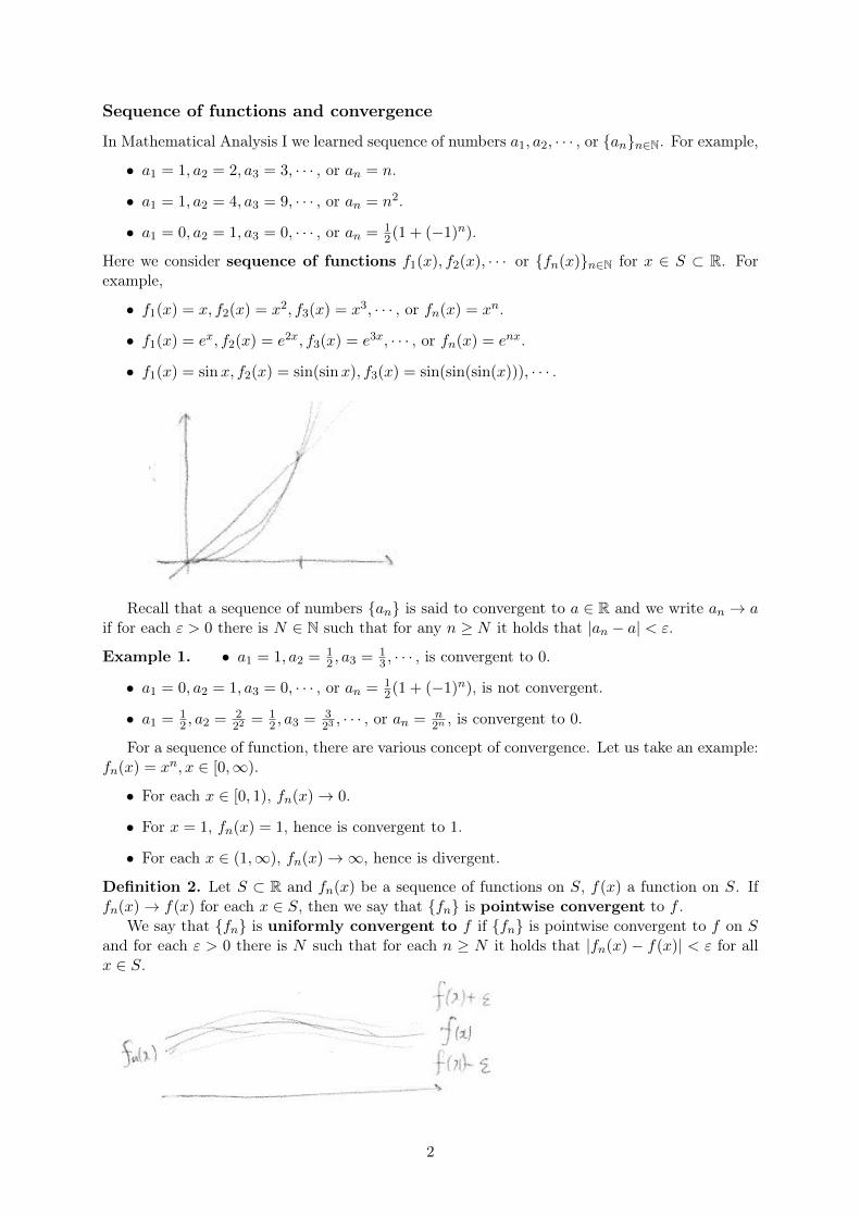
We say that {fn} is uniformly convergent to f if {fn} is pointwise convergent to f on Sand for each ε > 0 there is N such that for each n ≥ N it holds that |fn(x) − f(x)| < ε for allx ∈ S.
2
In the example above, {fn(x)} is uniformly convergent on [0, s] for any 0 < s < 1, but notuniformly convergent on [0, 1] (exercise).
Consider also fn(x) = e−nx2, x ∈ R. Where is it uniformly convergent and what is the limit?
Sequence of continuous functions
Let f(x) be a function on S ⊂ R. Recall that f is continuous at p ∈ S if for each ε > 0 there isδ > 0 such that |f(x)− f(p)| < ε for x ∈ S, |x− p| < δ. f is said to be continuous on S if it iscontinuous at each p ∈ S.
Theorem 3. Assume that fn → f uniformly on S and fn are continuous on S. Then f iscontinuous on S.
Proof. Let p ∈ S. For each ε > 0, by uniform convergence, there is N such that for n ≥ N itholds that |fn(x) − f(x)| < ε
3 for x ∈ S. By continuity of fN (x) at x = p, there is δ > 0 suchthat |fN (x)− fN (p)| < ε
3 . Therefore, for |x− p| < δ, we have
|f(x)− f(p)| = |f(x)− fN (x) + fN (x)− fN (p) + fn(p)− f(p)|
< |f(x)− fN (x)|+ |fN (x)− fN (p)|+ |fn(p)− f(p)| < 3 · ε3
= ε.
This is continuity of f at p. As p ∈ S is arbtrary, this shows continuity of f on S.
Recall that, if f is continuous on a closed interval [a, b], then we learned in Analysis I thatit is uniformly continuous: for each ε there is δ that |f(x) − f(y)| < ε whenever x, y ∈[a, b], |x−y| < δ. Furthermore, a continuous function on [a, b] has the absolute miminum andmaximum.
A step function s is a function such that s(x) = ak for x ∈ [xk, xk+1), where a = x1 < x2 <
· · · < xn = n. For a step function s, its integral is defined by∫ ba s(x)dx =
∑n−1k=1 ak(xk+1 − xk).
A function f on [a, b] is said to be integrable if
sups
∫ b
as(x)dx = inf
S
∫ b
aS(x)dx,
where the sup and inf are taken among step functions s(x) ≤ f(x) ≤ S(x) on S. In this case,the integral
∫ ba f(x)dx is defined to be the value of this equation above.
Recall that ∣∣∣∣∫ b
af(x)dx
∣∣∣∣ ≤ ∫ b
a|f(x)|dx ≤ (b− a) max
x∈[a,b]{|f(x)|}.
Theorem 4. Let {fn} be a sequence of continuous functions, uniformly convergent to f . Thenit holds that
limn→∞
∫ b
afn(x)dx =
∫ b
af(x)dx.
Proof. For ε > 0, by uniform convergence there is N such that for n ≥ N it holds that |fn(x)−f(x)| < ε
b−a . Then we obtain∣∣∣∣∫ b
afn(x)dx−
∫ b
af(x)dx
∣∣∣∣ ≤ ∫ b
a|fn(x)− f(x)|dx ≤ (b− a)
ε
b− a= ε.
This shows that limn→∞∫ ba fn(x)dx =
∫ ba f(x)dx.
3
Oct 25. Power series, Taylor series.
Series of functions, the Weierstrass M-test
Recall that, for a sequence {an} of numbers, the series∑an is the sequence {
∑nk=1 ak} of
numbers, consisting of partial sums. We say that a series∑an is convergent if {
∑nk=1 ak} is
convergent.In the same way, for a sequence of functions {fn}, we consider series of function
∑n fn.
This series is said to be pointwise convergent if {∑n
k=1 fk(x)} is pointwise convergent, uniformlyconvergent if {
∑nk=1 fk(x)} is uniformly convergent.
Just by replacing a sequence by a series, we obtain the following.
Theorem 5. Assume that series∑fn is convergent uniformly to g on S and fn are continuous
on S. Then g is continuous on S.Let {fn} be a sequence of continuous functions and
∑n fn uniformly convergent to g. Then
it holds that
limn→∞
∫ b
a
n∑k=1
fk(x)dx =
∫ b
ag(x)dx.
Proof. The same proofs apply, by noting that if fn’s are continuous, then∑n
k=1 fk is continuous.
Recall some test for convergence of series of numbers.
• (Ratio test) Let an > 0 and an+1
an→ L. If L < 1,
∑∞n=0 an converges. If L > 1,
∑∞n=0 an
diverges.
• (Root test) Let an > 0 and (an)1n → R. If R < 1,
∑∞n=0 an converges. If R > 1,
∑∞n=0 an
diverges.
• (Comparison test) Let an, bn > 0, c > 0 such that an < cbn. If∑∞
n=0 bn converges, so does∑∞n=0 an.
There is a useful criterion for uniform convergence.
Theorem 6 (The Weierstrass’s M-test). Let fn be a sequence of functions on S ⊂ R. If thereis a convergent series {Mn} of positive numbers such that |fn(x)| ≤Mn, then
∑fn is uniformly
convergent.
Proof. By comparison test,∑|fn(x)| is convergent for all x ∈ S, or in other words,
∑fn(x) is
pointwise absolutely convergent. Let f(x) be the limit.To see uniform convergence, we compute∣∣∣∣∣f(x)−
n∑k=1
fk(x)
∣∣∣∣∣ =
∣∣∣∣∣∞∑
k=n+1
fk(x)
∣∣∣∣∣ ≤∞∑k+1
|fk(x)| ≤∞∑k+1
Mk.
As∑
nMn is convergent, this last expression tends to 0 as k → ∞, independently of x. Thisshows uniform convergence.
Power series
Let an ∈ C be a sequence of complex numbers. We can consider the series (called a powerseries) ∑
n
anzn.
This may converge for some z, and diverge for other z.
4
Example 7. Simplest examples of power series.
• With an = 13n ,∑
nzn
3n is convergent for |z| < 3, and divervent for |z| > 3 (see the theorem
below). Indeed, by root test,(|z|n3n
) 1n
= |z|3 , and hence the series is convergent if |z|3 < 1
and divergent, say for positive z, if |z|3 > 1.
• With an = 1n! ,∑
nzn
n! is convergent for all z. Indeed, by ration test,(zn+1
(n+1)!
)/(zn
n!
)=
zn+1 → 0 for all z, therefore, the series is absolutely convergent for all z.
Theorem 8. Assume that∑anz
n converges for some z = z0 6= 0. Then for R < |z0|, the seriesconverges uniformly for z, |z| ≤ R and absolutely convergent.
Proof. If∑anz
n0 is convergent, then in particular |anzn0 | is bounded, namely, less than M for
some M > 0. Then, if |z| < R < |z0|, then |anzn| = |anzn0 | ·∣∣∣ zz0 ∣∣∣n < M Rn
|z0|n , whereRn
|z0|n < 1.
As∑M Rn
|z0|n is convergent (it is a geometric series), by the M-test, the series is uniformly andabsolutely convergent.
Theorem 9. Assume that∑anz
n converges for some z = z1 6= 0 and not convergent for z = z2.Then there is r > 0 such that
∑anz
n is convergent for |z| < r and divergent for |z| > r.
Proof. As there is z1, by Theorem 8, the series∑anz
n is convergent for |z| < |z1|. Let A bethe set of positive numbers R for which
∑anz
n is convergent if |z| < R. As there is z2, A is abounded set. Let r be the least upper bound. By definition, if |z| < r, then
∑anz
n is convergent.On the other hand, if |z3| > r and
∑anz
n3 is convergent, then by Theorem 8, the series must
converge for z with r < |z| < |z3|. Namely, |z| ∈ A. This contradicts with the definition of A,therefore,
∑anz
n is divergent for |z| > r.
This r is called the radius of convergence for the series∑anz
n. If the power series convergesfor all z ∈ C, the radius of convergence is∞ by convention. If it does not converge except z = 0,the radius of convergence is 0.
Derivative and integration of power series
Now let an ∈ R, x ∈ R. If∑anx
n converges, we can define a function by f(x) =∑∞
n=0 anxn.
We learned that it is not always possible to exchange limits and derivative or integration.For power series, the situation is better.
Theorem 10. Assume that, for all x ∈ (−r, r), the series f(x) =∑∞
n=0 anxn is convergent.
Then f(x) is continous and∫ x0 f(t)dt =
∑∞n=0
ann+1x
n+1.
Proof. Let us take R such that |x| < R < r. By Theorem 8, the series is uniformly convergentfor t ∈ [−R,R]. Then by Theorem 5, f(x) is continuous in [−R,R] and as x ∈ [−R,R], we canexchange the limit and integral, namely,∫ x
0f(t)dt =
∞∑n=0
∫ x
0ant
ndx =
∞∑n=0
ann+ 1
xn+1.
Theorem 11. Assume that, for all x ∈ (−r, r), the series f(x) =∑∞
n=0 anxn is convergent.
Then f(x) is differentiable and and f ′(x) =∑∞
n=1 nanxn.
5
Proof. In this case, r is smaller or equal to the radius of convergence. As |x| < r, we can taker0 such that |x| < r0 < r and then
∑∞n=1 nanx
n−1 =∑∞
n=1 nanrn0 · x
n−1
rn−10
. The series∑∞
n=1 anrn0
is absolutely convergent and n|x|n−1
rn−10
is bounded, hence by comparison test,∑∞
n=1 nanxn−1 is
(absolutely) convergent.This function g(x) =
∑∞n=1 nanx
n−1 is a power series with the coefficients nan. By Theorem10,∫ x0 g(x) =
∑∞n=1 anx
n = f(x)−a0. This shows that f(x) is differentiable by the fundamentaltheorem of calculus and f ′(x) = g(x) =
∑∞n=1 nanx
n−1.
Example 12. • As this is a geometric series, we know 1x+1 =
∑∞n=0(−1)nxn for |x| < 1. On
the other hand, (log(x+ 1))′ = 1x+1 . Hence log(x+ 1) =
∑∞n=0
(−1)nn+1 x
n+1.
• We know 1x2+1
=∑∞
n=0(−1)nx2n for |x| < 1. On the other hand, (arctanx)′ = 1x2+1
.
Hence arctanx =∑∞
n=0(−1)n2n+1 x
2n+1.
Set 30. Power series, Taylor series.
Shifted power series
Let {an} ⊂ C. Instead of∑anz
n, we can consider, for a ∈ C, a shifted power series∑an(z−a)n.
The theorem about the radius of convergence holds in a parallel way. If an, a ∈ R, then f(x) =∑nn=0 an(x− a)n defines a function on (a− r, a+ r), and the integral and differentiation can be
done term by term.In particular,
Theorem 13. Let f(x) =∑∞
n=0 an(x − a)n with x ∈ (a − r, a + r), where r is the radius ofconvergence. Then f (k)(x) =
∑∞n=k n(n− 1) · · · (n− k + 1)an(x− a)n−k.
Corollary 14. If f(x) =∑∞
n=0 an(x− a)n =∑∞
n=0 bn(x− a)n, then ak = bk = k!f (k)(a) for alln.
Proof. The n-th derivatives f (n)(a) are determined by the function f(x).
Taylor’s series
If f(x) is defined by f(x) =∑∞
n=0 an(x− a)n, then we saw an = f (n)(a)n! .
Question: If f(x) is infinitely many times differentiable, we can develop a power series (Taylor’sseries for f)
∑nn=0
f (n)
n! (x− a)n. Does it converge to f(x)?
Answer: not always. Consider f(x) =
{e−
1x = 0 (x > 0)
0 (x ≤ 0)(exercise).
Let En(x) := f(x) −∑n
k=0f (k)
k! (x − a)k be the error term of the n-th approximation. Welearned that En(x) = 1
n!
∫ xa (x − t)nf (n+1)(t)dt. One can prove this by integration by parts: for
example, with n = 2,
1
2
∫ x
a(x− t)2f (3)(t)dt =
1
2
[(x− t)2f (2)(t)
]xa
+
∫ x
a(x− t)f (2)(t)dt
= −1
2(x− a)2f (2)(a) +
[(x− t)f ′(t)
]xa
+
∫ x
af ′(t)dt
= −1
2(x− a)2f (2)(a)− (x− a)f ′(t) + f(x)− f(a) = E2(x).
There is a useful criterion for the convergence of Taylor’s series.
6
Theorem 15. If there is A, r ≥ 0 such that |f (n)(t)| ≤ An for t ∈ (a− r, a+ r), then En(x)→ 0as n→∞ for x ∈ (a− r, a+ r).
Proof. For x ≥ a, En(x) can be estimated as
|En(x)| ≤ 1
n!
∫ x
a|x− t|n|f (n+1)(t)|dt
≤ 1
n!
∫ x
a(x− t)nAndt
=1
(n+ 1)!
[−(x− t)n+1
]xa
=1
(n+ 1)!An(x− a)n+1
This tends to 0 as n→∞. A similar estimate can be made for x ≤ a.
Example 16. • f(x) = sinx. f (1)(x) = cosx, f (2)(x) = − sinx, f (3)(x) = − cosx, · · · ,|f (n)(x)| ≤ 1. Theorem 15 applies with a = 0 and sinx = x− 1
3!x3 + 1
5!x5 − · · · .
• Similarly, cosx = 1− 12!x
2 + 14!x
4 − · · · .
• f(x) = ex on x ∈ [−T, T ]. f (n)(x) = ex, hence |f (n)(x)| ≤ eT and Theorem 15 applies withx = 0. ex = 1 + x+ 1
2!x2 + 1
3!x3 + · · · .
Applications to ordinary differential equations
An ordinary differential equation is an equation about a function y(x) instead of a number x.For example, −2y(x) = (1 − x2)y′′(x). Such equations can be sometimes solved using powerseries.Problem: Find a function y(x) such that −2y(x) = (1− x2)y′′(x) with y(0) = 1, y′(0) = 1.Solution:
Step 1. Assume that y(x) =∑∞
n=0 anxn. Then
y′(x) =∞∑n=1
nanxn−1, y′′(x) =
∞∑n=2
n(n− 1)anxn−2.
Step 2. y(x) must satisfy
−2y(x) = −2∞∑n=0
anxn = (1− x2)y′′(x)
= (1− x2)∞∑n=2
n(n− 1)anxn−2
=
∞∑n=2
n(n− 1)anxn−2 −
∞∑n=2
n(n− 1)anxn
=
∞∑n=0
(n+ 2)(n+ 1)an+2xn −
∞∑n=0
n(n− 1)anxn
Step 3. By Corollary 14, −2an = (n + 2)(n + 1)an+2 − n(n − 1)an. Equivalently, (n + 2)(n +1)an+1 = [n(n− 1)− 2]an = (n+ 1)(n− 2)an, or an+2 = n−2
n+2an.
Step 4. −a0 = a2, a4 = 0 = a6 · · · . a3 = −13a1, a5 = 1
5a3 = − 15·3a1, a7 = 3
7a5 = − 17·5a1, in
general, a2n+1 = − a1(2n+1)(2n−1) .
Step 5. By y(0) = 1, a0 = 1 and y′(0) = 1, a1 = 1. Hence y(x) = 1−x2+∑∞
n=01
(2n+1)(2x−1)x2n+1.
Step 6. This is convergent for |x| < 1.
7
Binominal series
For α ∈ R, n ∈ N, we define (α
n
)=α(α− 1) · · · (α− n+ 1)
n!.
Theorem 17. (1 + x)α =∑n
n=0
(αn
)xn for |x| < 1.
Proof. By ratio test,∣∣∣( αn+1
)|x|n+1
∣∣∣ / ∣∣(αn)|x|n∣∣ = |α − n + 1||x|/n → |x|, the right-hand sideconverges for |x| < 1.
Put f(x) = (1+x)α, then f ′(x) = α(1+x)α−1 = α f(x)1+x and f(0) = 1. Put g(x) =∑∞
n=0
(αn
)xn.
(x+ 1)g′(x) =∑∞
n=1 n(αn
)xn−1(x+ 1) =
∑∞n=1[n
(αn
)+ (n+ 1)
(αn+1
)]xn = αg(x), and g(0) = 1.
Therefore, f(x) and g(x) satisfy the same first-order differential equation and f(0) = g(0) =1, hence f(x) = g(x). Namely, (1 + x)α =
∑∞n=0
(αn
)xn for |x| < 1.
Oct 02. Scalar and vector fields.
Higher dimensional space
Let xxx = (x1, x2, · · · , xn) ∈ Rn. We define the inner product xxx ·yyy =∑n
k=1 xkyk ∈ R and the norm
‖xxx‖ =√xxx · xxx =
√∑nk=1 x
2k. In linear algebra we leaned
|xxx · yyy| ≤ ‖xxx‖ · ‖yyy‖ (Cauchy-Schwarz inequality)‖x+ yx+ yx+ y‖ ≤ ‖xxx‖+ ‖yyy‖ (Triangle inequality)
A map FFF : Rn → Rm is called a “field”. The case m = 1 is a scalar field, and in general itis a vector field.
Some examples have practical applications:
• T : R3 ⊃ S → R, temperature in a room
• VVV : R3 ⊃ S → R3, wind velocity
• EEE : R3 ⊃ S → R3, electric field.
We denote fff(x1, · · · , xn) by fff(xxx), and they represent the same vector field Rn → Rm.
Open balls and open sets
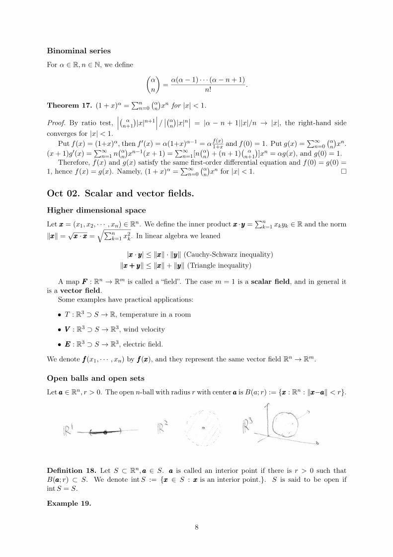
Let aaa ∈ Rn, r > 0. The open n-ball with radius r with center aaa isB(a; r) := {xxx : Rn : ‖xxx−aaa‖ < r}.
Definition 18. Let S ⊂ Rn, aaa ∈ S. aaa is called an interior point if there is r > 0 such thatB(aaa; r) ⊂ S. We denote intS := {xxx ∈ S : xxx is an interior point.}. S is said to be open ifintS = S.
Example 19.
8
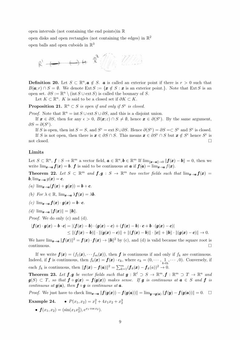
open intervals (not containing the end points)in Ropen disks and open rectangles (not containing the edges) in R2
open balls and open cuboids in R3
Definition 20. Let S ⊂ Rn, aaa /∈ S. aaa is called an exterior point if there is r > 0 such thatB(aaa; r) ∩ S = ∅. We denote ExtS := {xxx /∈ S : xxx is an exterior point.}. Note that ExtS is anopen set. ∂S := Rn \ (intS ∪ extS) is called the bounary of S.
Let K ⊂ Rn. K is said to be a closed set if ∂K ⊂ K.
Proposition 21. Rn ⊂ S is open if and only if Sc is closed.
Proof. Note that Rn = intS ∪ extS ∪ ∂S, and this is a disjoint union.If xxx ∈ ∂S, then for any ε > 0, B(xxx; ε) ∩ S 6= ∅, hence xxx ∈ ∂(Sc). By the same argument,
∂S = ∂(Sc).If S is open, then intS = S, and Sc = extS∪∂S. Hence ∂(Sc) = ∂S =⊂ Sc and Sc is closed.If S is not open, then there is xxx ∈ ∂S ∩ S. This means xxx ∈ ∂Sc ∩ S but xxx /∈ Sc hence Sc is
not closed.
Limits
Let S ⊂ Rn, fff : S → Rm a vector field, aaa ∈ Rn, bbb ∈ Rm If lim‖xxx−aaa‖→0 ‖fff(xxx) − bbb‖ = 0, then wewrite limxxx→aaa fff(xxx) = bbb. fff is said to be continuous at aaa if fff(aaa) = limxxx→aaa f(xxx).
Theorem 22. Let S ⊂ Rm and fff,ggg : S → Rm two vector fields such that limxxx→aaa fff(xxx) =bbb, limxxx→aaa g(xxx) = ccc.
(a) limxxx→aaa(fff(xxx) + ggg(xxx)) = bbb+ ccc.
(b) For λ ∈ R, limxxx→aaa λfff(xxx) = λbbb.
(c) limxxx→aaa fff(xxx) · ggg(xxx) = bbb · ccc.
(d) limxxx→aaa ‖fff(xxx)‖ = ‖bbb‖.Proof. We do only (c) and (d).
|fff(xxx) · ggg(xxx)− bbb · ccc| = |(fff(xxx)− bbb) · (ggg(xxx)− ccc) + (fff(xxx)− bbb) · ccc+ bbb · (ggg(xxx)− ccc)|≤ ‖(fff(xxx)− bbb)‖ · ‖(ggg(xxx)− ccc)‖+ ‖(fff(xxx)− bbb)‖ · ‖ccc‖+ ‖bbb‖ · ‖(ggg(xxx)− ccc)‖ → 0.
We have limxxx→aaa ‖fff(xxx)‖2 = fff(xxx) · fff(xxx)→ ‖bbb‖2 by (c), and (d) is valid because the square root iscontinuous.
If we write fff(xxx) = (f1(xxx), · · · fm(xxx)), then fff is continuous if and only if fk are continuous.Indeed, if fff is continuous, then fk(xxx) = fff(xxx) · ek, where ek = (0, · · · , 1
k-th, · · · , 0). Conversely, if
each fk is continuous, then ‖fff(xxx)− fff(aaa)‖2 =∑m
k=1(fffk(xxx)− fffk(a))2 → 0.
Theorem 23. Let fff,ggg be vector fields such that ggg : R` ⊃ S → Rm, fff : Rm ⊃ T → Rn andggg(S) ⊂ T , so that fff ◦ ggg(xxx) = fff(ggg(xxx)) makes sense. If ggg is continuous at aaa ∈ S and fff iscontinuous at ggg(aaa), then fff ◦ ggg is continuous at aaa.
Proof. We just have to check limxxx→aaa ‖fff(ggg(xxx))− fff(ggg(aaa))‖ = limyyy→ggg(aaa) ‖fff(yyy)− fff(ggg(aaa))‖ = 0.
Example 24. • P (x1, x2) = x21 + 4x1x2 + x32
• fff(x1, x2) = (sin(x1x22), e
x1 cosx2).
9
Oct 07. Derivatives of scalar fields.
Directional derivatives
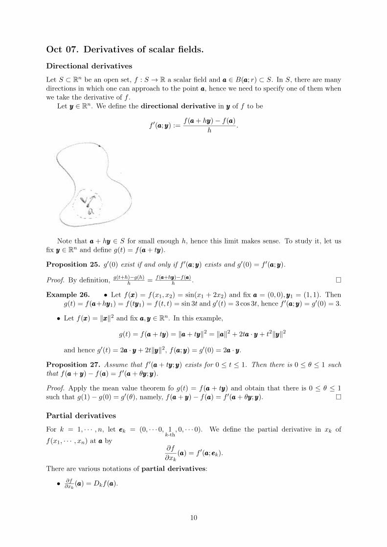
Let S ⊂ Rn be an open set, f : S → R a scalar field and aaa ∈ B(aaa; r) ⊂ S. In S, there are manydirections in which one can approach to the point aaa, hence we need to specify one of them whenwe take the derivative of f .
Let yyy ∈ Rn. We define the directional derivative in yyy of f to be
f ′(aaa;yyy) :=f(aaa+ hyyy)− f(aaa)
h.
Note that aaa + hyyy ∈ S for small enough h, hence this limit makes sense. To study it, let usfix yyy ∈ Rn and define g(t) = f(aaa+ tyyy).
Proposition 25. g′(0) exist if and only if f ′(aaa;yyy) exists and g′(0) = f ′(aaa;yyy).
Proof. By definition, g(t+h)−g(h)h = f(aaa+hyyy)−f(aaa)h .
Example 26. • Let f(xxx) = f(x1, x2) = sin(x1 + 2x2) and fix aaa = (0, 0), yyy1 = (1, 1). Theng(t) = f(aaa+hyyy1) = f(tyyy1) = f(t, t) = sin 3t and g′(t) = 3 cos 3t, hence f ′(aaa;yyy) = g′(0) = 3.
• Let f(xxx) = ‖xxx‖2 and fix aaa,yyy ∈ Rn. In this example,
g(t) = f(aaa+ tyyy) = ‖aaa+ tyyy‖2 = ‖aaa‖2 + 2taaa · yyy + t2‖yyy‖2
and hence g′(t) = 2aaa · yyy + 2t‖yyy‖2, f(aaa;yyy) = g′(0) = 2aaa · yyy.
Proposition 27. Assume that f ′(aaa + tyyy;yyy) exists for 0 ≤ t ≤ 1. Then there is 0 ≤ θ ≤ 1 suchthat f(aaa+ yyy)− f(aaa) = f ′(aaa+ θyyy;yyy).
Proof. Apply the mean value theorem fo g(t) = f(aaa + tyyy) and obtain that there is 0 ≤ θ ≤ 1such that g(1)− g(0) = g′(θ), namely, f(aaa+ yyy)− f(aaa) = f ′(aaa+ θyyy;yyy).
Partial derivatives
For k = 1, · · · , n, let eeek = (0, · · · 0, 1k-th
, 0, · · · 0). We define the partial derivative in xk of
f(x1, · · · , xn) at aaa by∂f
∂xk(aaa) = f ′(aaa;eeek).
There are various notations of partial derivatives:
• ∂f∂xk
(aaa) = Dkf(aaa).
10
• If we consider R2, then the scalar field is often written as f(x, y) and one denotes ∂f∂x (aaa) =
D1f(aaa), ∂f∂y (aaa) = D2f(aaa). Similarly, if we are in R3, then for f(x, y, z) we also denote∂f∂z (aaa) = D3f(aaa).
If Dkf exists, one can also consider D`(Dkf) = ∂2f∂x`∂xk
, and even higher partial derivatives.In general D`Dkf 6= DkD`f .
In practice, in order to compute the partial derivative ∂f∂xk
, one should consider all otherx`, ` 6= k as constants and take the derivative with respect to xk.
Example 28. • (Good function) Let us take f(x, y) = x2 + 3xy + y4. Then ∂f∂x (x, y) =
D1f(x, y) = 2x+ 3y, ∂f∂y (x, y) = D2f(x, y) = 3x+ 4y3. Further, ∂2f∂x2
(x, y) = 2, ∂2f
∂y∂x(x, y) =∂2f∂x∂y (x, y) = 3, ∂
2f∂y2
(x, y) = 12y2.
• (Bad function) Consider f(x, y) =
{xy2
x2+y4if x 6= 0
0 if x = 0. Let bbb = (b, c) where b 6= 0, then
f ′((0, 0);bbb) = limh→0bc2h3
(b2h2+c4h4)h= bc2. Similarly, if bbb = (0, c), then f ′((0, 0);bbb) =
limh→00
c4h4= 0. Therefore, all the directional derivatives exist. However, if we take
f(t2, t) = t4
2t4= 1
2 , hence f(x, y) is not continuous at (0, 0).
Total derivatives
Recall that, in R1, if f(x) is differentiable, then we have
f(a+ h) = f(a) + hf ′(a) + hE(a, h)
and E(a, h) → 0 as h → 0. In other words, f(x) can be approximated by f(a) + hf ′(a) to thefirst order in h around a.
Definition 29. Let S ⊂ Rn be open, f : S → R a scalar field. We say that f is differentiableat aaa ∈ S if there is Taaa ∈ Rn and E(aaa,vvv) such that
f(aaa+ vvv) = f(aaa) + Taaa · vvv + ‖vvv‖E(aaa,vvv)
for vvv ∈ B(aaa; r) and E(aaa,vvv)→ 0 as vvv → 000. Taaa is called the total derivative of f at aaa.
Theorem 30. If f is differentiable at aaa, then Taaa = (D1f(aaa), · · ·Dnf(aaa)) and f ′(aaa;yyy) = Taaa · yyy.
Proof. As f is differentiable at aaa, it holds that f(aaa+vvv) = f(aaa)+Taaa ·vvv+‖vvv‖E(aaa,vvv) where E(aaa,vvv)as vvv → 000. Let us take vvv = hyyy. Then
f ′(aaa;yyy) =f(aaa+ hyyy)− f(aaa)
h=Taaa · hyyy + h‖yyy‖E(aaa, hyyy)
h= Taaa · yyy + ‖yyy‖E(aaa, hyyy)→ Taaa · yyy.
Especially, if aaa = eeek, then Dkf(aaa) = Taaa ·eeek. Therefore, we have Taaa = (D1f(aaa), · · · , Dnf(aaa)).
Taaa = (D1f(aaa), · · · , Dnf(aaa)) =: ∇f(aaa) is called the gradient of f at aaa.
Proposition 31. If f is differentiable at aaa, then it is continuous at aaa.
Proof. We just have to estimate
|f(aaa+ vvv)− f(aaa)| = |Taaa · vvv + ‖vvv‖E(aaa,vvv)| ≤ ‖Taaa‖‖vvv‖+ ‖vvv‖|E(aaa,vvv)| → 0.
11
Theorem 32. Assume that D1f, · · ·Dnf exist in B(aaa; r) and are continuous at aaa. Then f isdifferentiable at aaa.
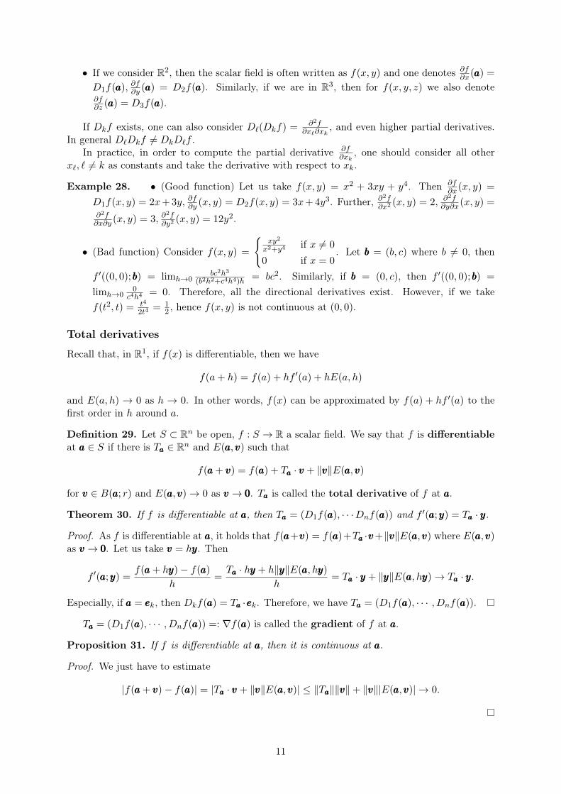
Proof. Let us write vvv = (v1, · · · vn) and introduce uuuk = (v1, · · · , vk, 0, · · · , 0) with uuu0 = (0, · · · , 0).Note that uuuk − uuuk−1 = vkeeek. Then we have
f(aaa+ vvv)− f(aaa) =
n∑k=1
(f(aaa+ uuuk)− f(aaa+ uuuk−1))
=
n∑k=1
vkf′(aaa+ uuuk−1 + θkvkeeek;eeek)
=
n∑k=1
vkf′(aaa+ uuuk−1;eeek) +
n∑k=1
vk(f′(aaa+ uuuk−1 + θkvkeeek;eeek)− f ′(aaa+ uuuk−1;eeek))
=
n∑k=1
vkf′(aaa+ uuuk−1;eeek) + ‖vvv‖
n∑k=1
vk‖vvv‖
(Dkf(aaa+ uuuk−1 + θkvkeeek)−Dkf(aaa)).
As we have E(aaa,vvv) =∑n
k=1vk‖vvv‖(Dkf(aaa+uuuk−1 + θkvkeeek)−Dkf(aaa)), this tends to 0 as vvv → 000 and∑n
k=1 vkf′(aaa+ uuuk−1;eeek)→ ∇f(aaa) · vvv.
Oct 09. Tangent and chain rule.
Parametrized curves
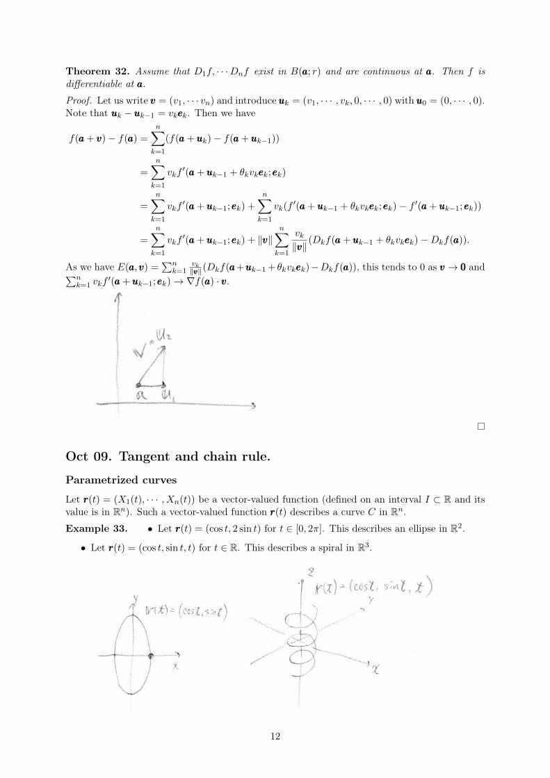
Let rrr(t) = (X1(t), · · · , Xn(t)) be a vector-valued function (defined on an interval I ⊂ R and itsvalue is in Rn). Such a vector-valued function rrr(t) describes a curve C in Rn.Example 33. • Let rrr(t) = (cos t, 2 sin t) for t ∈ [0, 2π]. This describes an ellipse in R2.
• Let rrr(t) = (cos t, sin t, t) for t ∈ R. This describes a spiral in R3.
12
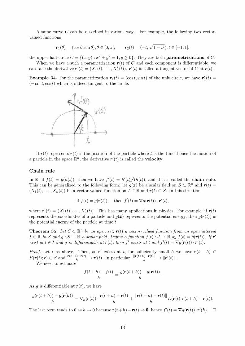
A same curve C can be described in various ways. For example, the following two vector-valued functions
rrr1(θ) = (cos θ, sin θ), θ ∈ [0, π], rrr2(t) = (−t,√
1− t2), t ∈ [−1, 1].
the upper half-circle C = {(x, y) : x2 + y2 = 1, y ≥ 0}. They are both parametrizations of C.When we have a such a parametrization rrr(t) of C and each component is differentiable, we
can take the derivative rrr′(t) = (X ′1(t), · · · , X ′n(t)). rrr′(t) is called a tangent vector of C at rrr(t).
Example 34. For the parametrirzation rrr1(t) = (cos t, sin t) of the unit circle, we have rrr′1(t) =(− sin t, cos t) which is indeed tangent to the circle.
If rrr(t) represents rrr(t) is the position of the particle where t is the time, hence the motion ofa particle in the space Rn, the derivative rrr′(t) is called the velocity.
Chain rule
In R, if f(t) = g(h(t)), then we have f ′(t) = h′(t)g′(h(t)), and this is called the chain rule.This can be generalized to the following form: let g(xxx) be a scalar field on S ⊂ Rn and rrr(t) =(X1(t), · · · , Xn(t)) be a vector-valued function on I ⊂ R and rrr(t) ⊂ S. In this situation,
if f(t) = g(rrr(t)), then f ′(t) = ∇g(rrr(t)) · rrr′(t),
where rrr′(t) = (X ′1(t), · · · , X ′n(t)). This has many applications in physics. For example, if rrr(t)represents the coordinates of a particle and g(xxx) represents the potential energy, then g(rrr(t)) isthe potential energy of the particle at time t.
Theorem 35. Let S ⊂ Rn be an open set, rrr(t) a vector-valued function from an open intervalI ⊂ R in S and g : S → R a scalar field. Define a function f(t) : J → R by f(t) = g(rrr(t)). If rrr′
exist at t ∈ I and g is differentiable at rrr(t), then f ′ exists at t and f ′(t) = ∇g(rrr(t)) · rrr′(t).
Proof. Let t as above. Then, as rrr′ exists at t, for sufficiently small h we have rrr(t + h) ∈B(rrr(t); r) ⊂ S and rrr(t+h)−rrr(t)
h → rrr′(t). In particular, ‖rrr(t+h)−rrr(t)‖h → ‖rrr′(t)‖.We need to estimate
f(t+ h)− f(t)
h=g(rrr(t+ h))− g(rrr(t))
h.
As g is differentiable at rrr(t), we have
g(rrr(t+ h))− g(rrr(h))
h= ∇g(rrr(t)) · r
rr(t+ h)− rrr(t)h
+‖rrr(t+ h)− rrr(t)‖
hE(rrr(t);rrr(t+ h)− rrr(t)).
The last term tends to 0 as h→ 0 because rrr(t+h)−rrr(t)→ 000, hence f ′(t) = ∇g(rrr(t)) ·rrr′(h).
13
Example 36. Let xxx = (x, y, z) ∈ R, g(xxx) = − 1‖xxx‖ , rrr(t) = (t, 0, 0), f(t) = g(rrr(t)). We have
∇g(xxx) = ( x‖xxx‖3 ,
y‖xxx‖3 ,
z‖xxx‖3 ) and rrr′(t) = (1, 0, 0). Then, for t > 0, ∇g(rrr(t)) = ( 1
t2, 0, 0) and
f ′(t) = 1t2.
The chain rule can be applied to compute the derivative of some function on R.
Example 37. • f(t) = tt for t > 0. With g(x, y) = xy and rrr(t) = (t, t), we have f(t) =g(rrr(t)). As ∇g(x, y) = (yxy−1, log xxy) and rrr′(t) = (1, 1), we have f ′(t) = ∇g(rrr(t)) ·rrr′(t) =tt + log t · tt.
• f(t) =∫ t2−t4 e
s2ds. We do not know the indefinite integral of es2 . However, we put itF (x, y) =
∫ yx e
s2ds. Then, f(t) = F (−t4, t2) = F (rrr(t)), where rrr(t) = (−t4, t2). Withrrr′(t) = (−4t3, 2t2) and D1F (x, y) = −ex2 , D2F (x, y) = ey
2 , we have f ′(t) = 2t2et2
+ 4t3et2 .
Level sets
Let f be a non-constant scalar field on S ⊂ R2. Assume that c ∈ R and the equation f(x, y) = cdefines a curve in R and it has a tangent at each of its point. Then it holds that
• The gradient vector ∇f(aaa) is normal to C if aaa ∈ C. Indeed, assume that C can be writtenas rrr(t). Then, as f is constant along C, we have d
dtf(rrr(t)) = ∇f(rrr(t)) · rrr′(t) = 0. As rrr′(t)is a tangent vector to C, ∇f(rrr(t)) is normal to C.
• The directional derivative of f is 0 along C, and it has the largest value in the direction of∇f(rrr(t)).
The tangent line at aaa = (a, b) is represented by the equation
D1f(aaa)(x− a) +D2f(aaa)(y − b) = 0.
Indeed, this passes through (a, b) and is orthogonal to ∇f(aaa) = (D1f(aaa), D2f(aaa)).More generally, if f is a scalar field on S ⊂ Rn and c ∈ R, L(c) = {xxx ∈ S : f(xxx) = c} is called
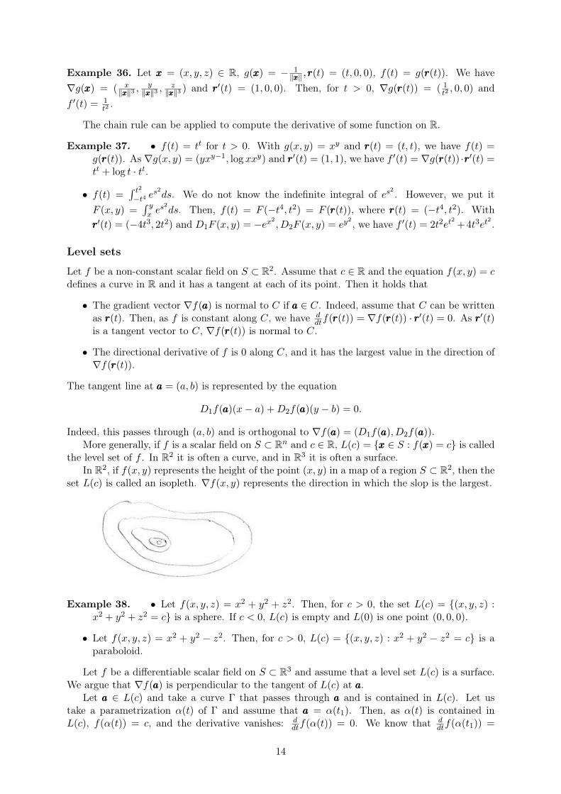
the level set of f . In R2 it is often a curve, and in R3 it is often a surface.In R2, if f(x, y) represents the height of the point (x, y) in a map of a region S ⊂ R2, then the
set L(c) is called an isopleth. ∇f(x, y) represents the direction in which the slop is the largest.
Example 38. • Let f(x, y, z) = x2 + y2 + z2. Then, for c > 0, the set L(c) = {(x, y, z) :x2 + y2 + z2 = c} is a sphere. If c < 0, L(c) is empty and L(0) is one point (0, 0, 0).
• Let f(x, y, z) = x2 + y2 − z2. Then, for c > 0, L(c) = {(x, y, z) : x2 + y2 − z2 = c} is aparaboloid.
Let f be a differentiable scalar field on S ⊂ R3 and assume that a level set L(c) is a surface.We argue that ∇f(aaa) is perpendicular to the tangent of L(c) at aaa.
Let aaa ∈ L(c) and take a curve Γ that passes through aaa and is contained in L(c). Let ustake a parametrization α(t) of Γ and assume that aaa = α(t1). Then, as α(t) is contained inL(c), f(α(t)) = c, and the derivative vanishes: d
dtf(α(t)) = 0. We know that ddtf(α(t1)) =
14
∇f(ααα(t1)) · ααα′(t1). Therefore, the tangent vector ααα′(t1) is orthogonal to ∇f(ααα(t1)). This holdsfor any curve passing through aaa and contained in L(c), hence ∇f(ααα(t1)) is perpendicular to thetangent plane of f .
The tangent plane at aaa = (a, b, c) is represented by the equation
D1f(aaa)(x− a) +D2f(aaa)(y − b) +D3f(aaa)(z − c) = 0.
Oct 14. Derivatives of vector fields.
Let fff : Rn ⊃ S → Rm be a vector field. For aaa ∈ S and yyy ∈ Rn, we define, as before, thedirectional derivative by
fff ′(aaa;yyy) = limh→0
fff(aaa+ hyyy)− fff(aaa)
h.
fff ′(aaa;yyy) is a vector in Rn. This means that, if fff = (f1, · · · , fn), then the directional derivative isfff ′(aaa;yyy) = (f ′1(aaa;yyy), · · · , f ′n(aaa;yyy)).
Dkfff(aaa) = ∂fff∂xk
(aaa) = fff ′(aaa;eeek) as with scalar fields. In R3, we often write fff = (fx, fy, fz).
Example 39. Let EEE(x, y, z, t),BBB(x, y, z, t) be electric and magnetic fields. They are vector fieldsR4 → R3.
• ∂Ex∂x +
∂Ey
∂y + ∂Ez∂z = 4πρ (Gauss’ law).
• ∂Bx∂x +
∂By
∂y + ∂Bz∂z = 0 (absence of magnetic charge).
Similarly to the case of scalar field, we say that fff is differentiable at aaa if there is a lineartranformation Taaa : Rn ∈ Rm and EEE(aaa,vvv) such that
fff(aaa+ vvv) = fff(aaa) + TTTaaa(vvv) + ‖vvv‖E(aaa,vvv)
for vvv ∈ B(aaa; r) and EEE(aaa,vvv)→ 000 as vvv → 000. We also have
Theorem 40. If fff is differentiable at aaa, then fff is continuous at aaa and TTTaaa(yyy) = fff ′(aaa;yyy).
We omit the proof, as it is parallel to the case of scalar fields.Recall that a linear transformation Rn → Rm can be written as a matrix if we fix a basis.
We write TTTaaa as
TTTaaa =
D1f1(aaa) D2f1(aaa) · · · Dnf1(aaa)D1f2(aaa) D2f2(aaa) · · · Dnf2(aaa)
......
...D1fm(aaa) D2fm(aaa) · · · Dnfm(aaa)
and called the Jacobian matrix of fff at aaa. It is sometimes denoted by Taaa = fff ′(aaa).
Example 41. Linear transformation. Let fff(x, y) = (ax+ by, cx+ dy), then TTTaaa =
(a bc d
)Chain rule for vector fields
Note that, for a linear operator T : Rn → Rm, ‖T (vvv)‖ ≤M‖v‖ for some M > 0. Indeed, we canwrite T (v) =
∑mk=1uuuk〈eeek, v〉 and hence ‖T (v)‖ ≤
∑‖uuuk‖ · ‖v‖.
Theorem 42. Let fff : Rn ⊃ S → T ⊂ Rm and ggg : Rm ⊃ T → R`. If fff is differentiable ataaa ∈ S and ggg is differentiable at fff(aaa). Then hhh = ggg ◦ fff : S → R` is differentiable at aaa andhhh′(aaa) = ggg′(fff(aaa)) ◦ fff ′(aaa), the composition of linear operators.
15
Proof. We consider the difference hhh(aaa+yyy)−hhh(aaa) = ggg(fff(aaa+yyy))−ggg(fff(aaa)). By the differentiablityof ggg and fff , there are EEEggg,EEEfff such that
hhh(aaa+ yyy)− hhh(aaa)
= ggg(fff(aaa+ yyy))− ggg(fff(aaa))
= ggg′(fff(aaa))(fff(aaa+ yyy)− fff(aaa)) + ‖fff(aaa+ yyy)− fff(aaa)‖EEEggg(fff(aaa), fff(aaa+ yyy)− fff(aaa))
= ggg′(fff(aaa))(fff ′(aaa)(yyy) + ‖yyy‖EEEfff (aaa,yyy)) + ‖fff(aaa+ yyy)− fff(aaa)‖EEEggg(fff(aaa), fff(aaa+ yyy)− fff(aaa))
= ggg′(fff(aaa))(fff ′(aaa)(yyy)) + ggg′(fff(aaa))(‖yyy‖EEEfff (aaa,yyy)) + ‖fff(aaa+ yyy)− fff(aaa)‖EEEggg(fff(aaa), fff(aaa+ yyy)− fff(aaa))
and as yyy → 000, ‖yyy‖ → 0 and fff(aaa+ yyy)− fff(aaa)→ 000, moreover, ‖fff(aaa+yyy)−fff(aaa)‖‖y‖ is bounded. Hence bydefinition, hhh is differentiable and hhh′(aaa) = ggg′(fff(aaa)) ◦ fff ′(aaa).
Polar coordinates
An example of composition of vector field is given by a change of coordinages. Let g(x, y) bea scalar field, and x = X(r, θ) = r cos θ, y = Y (r, θ) = r sin θ be the polar coordinate, the mapfff(r, θ) = (X(r, θ), Y (r, θ)) can be considered as a vector field from R+× [0, 2π)→ R2. We wouldlike to compute derivatives of ϕ(r, θ) = g(X(r, θ), Y (r, θ)).
By the chain rule, g′(xxx) = ( ∂g∂x ,∂g∂y ) and
fff ′(r, θ) =
(∂X∂r
∂X∂θ
∂Y∂r
∂Y∂θ
)=
(cos θ −r sin θsin θ r cos θ
)we obtain
∂ϕ
∂r(r, θ) =
∂g
∂x(r cos θ, r sin θ) cos θ +
∂g
∂y(r cos θ, r sin θ) sin θ
∂ϕ
∂θ(r, θ) = −∂g
∂x(r cos θ, r sin θ)r sin θ +
∂g
∂y(r cos θ, r sin θ)r cos θ
This can also be written as
∂ϕ
∂r(r, θ) cos θ − 1
r
∂ϕ
∂θ(r, θ) sin θ =
∂f
∂x(r cos θ, r sin θ)
∂ϕ
∂r(r, θ) sin θ +
1
r
∂ϕ
∂θ(r, θ) cos θ =
∂f
∂y(r cos θ, r sin θ)
Sufficient condition for equality of mixed partial derivatives
Let f be a scalar field. In general, D1D2f 6= D2D1f . Let us take
f(x, y) =xy(x2 − y2)x2 + y2
for (x, y) 6= (0, 0), 0 for (x, y) = (0, 0).
Then D1f(x, y) = y(x4+4x2y2−y4)(x2+y2)2
for (x, y) 6= (0, 0) and D1f(0, 0) = limh→00−0h = 0. Then,
D2D1f(0, 0) = limh→0h·(−h4)h4·h = −1. Similarly, D1D2f(0, 0) = 1, so D1D2f 6= D2D1f .
Theorem 43. Let f be a scalar field and assume that D1f,D2, D1D2, D2D1f exist in an openset S. If (a, b) ∈ S and D1D2f,D2D1f are both continuous at (a, b), then D1D2f(a, b) =D2D1f(a, b).
16
Proof. By the mean value theorem applied to G(x) = f(x, b + k) − f(x, b), G′(x) = D1f(x, b +k)−D1f(x, b),
(f(a+ h, b+ k)− f(a+ h, b))− (f(a, b+ k)− f(a, b))
= hG′(a+ θ1h)
= h(D1f′(a+ θ1h, b+ k)−D1f
′(a+ θ1h, b))
= hkD2D1f(a+ θ1h, b+ ϕ1k),
where 0 ≤ θ, ϕ ≤ 1, and we applied the mean value theorem toD1f(a+θ1h, y) = H(y). Similarly,(f(a+ h, b+ k)− f(a+ h, b))− (f(a, b+ k)− f(a, b)) = hkD1D2f(a+ θ2h, b+ ϕ2k), hence
D1D2f(a+ θ2h, b+ ϕ2k) = D2D1f(a+ θ2h, b+ ϕ2k).
As h, k → 0, this shows D1D2f(a, b) = D2D1f(a, b).
Oct 16. Partial differential equations.
A partial differential equation is an equation about a scalar field or a vector field involving itspartial derivatives.
Example 44. Some (linear) partial differential equations.
• ∂f∂t (x, t) = k ∂
2f∂x2
(x, y), where k is a constant (heat equation)
• ∂2f∂x2
(x, y) + ∂2f∂y2
(x, y) = 0 (Laplace’s equation)
• ∂2f∂x2
(x, t)− c2 ∂2f∂t2
(x, t) = 0, where c is a constant (wave equation)
Maxwell’s equations, Navier-Stokes equations, Einstein’s equations...
In general, PDE’s have many solutions, and need to specify a boundary condition (or aninitial condition):
Consider ∂f∂x (x, y) = 0. For any function g(y), f(x, y) = g(y) is a solution, and it holds that
f(0, y) = g(y). In general, such a condition is called a boundary condition.
First order linear PDE
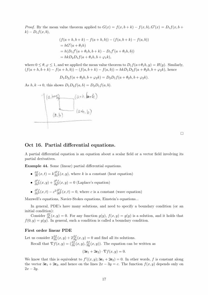
Let us consider 3∂f∂x (x, y) + 2∂f∂y (x, y) = 0 and find all its solutions.Recall that ∇f(x, y) = (∂f∂x (x, y), ∂f∂y (x, y)). The equation can be written as
(3eee1 + 2eee2) · ∇f(x, y) = 0.
We know that this is equivalent to f ′((x, y); 3eee1 + 2eee2) = 0. In other words, f is constant alongthe vector 3eee1 + 2eee2, and hence on the lines 2x− 3y = c. The function f(x, y) depends only on2x− 3y.
17
Actually, if g is any differentiable function, f(x, y) = g(2x− 3y) is a solution. Indeed, by thechain rule, ∂f∂x (x, y) = 2g′(2x−3y), ∂f∂y (x, y) = −3g′(2x−3y) and hence 3∂f∂x (x, y)+2∂f∂y (x, y) = 0.Therefore, we have proved that a general solution is g(2x− 3y) for some differentiable functiong.
Conversely, a general solution is of the form g(2x− 3y). Indeed, let u = 2y− x, v = 2x− 3y.This can be solved: x = 3u+ 2v, y = 2u+ v Define h(u, v) = f(3u+ 2v, 2u+ v). We have
∂h
∂u(u, v) = 3
∂f
∂x(3u+ 2v, 2u+ v) + 2
∂f
∂y(3u+ 2v, 2u+ v) = 0.
Namely, h is only a function of v: h(u, v) = g(v). Or f(x, y) = g(2x− 3y).With the same method, we can prove
Theorem 45. Let g be a differentiable function, a, b ∈ R, (a, b) 6= (0, 0). Define f(x, y) =g(bx− ay). Then f satisfies the equation
a∂f
∂x(x, y) + b
∂f
∂y(x, y) = 0. (1)
Conversely, every solution of (1) is of the form g(bx− ay).
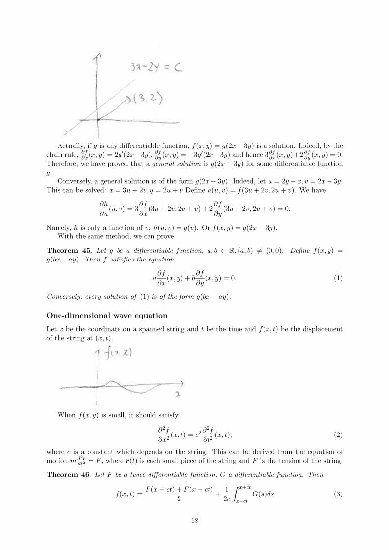
One-dimensional wave equation
Let x be the coordinate on a spanned string and t be the time and f(x, t) be the displacementof the string at (x, t).
When f(x, y) is small, it should satisfy
∂2f
∂x2(x, t) = c2
∂2f
∂t2(x, t), (2)
where c is a constant which depends on the string. This can be derived from the equation ofmotion md2rrr
dt2= F , where rrr(t) is each small piece of the string and F is the tension of the string.
Theorem 46. Let F be a twice differentiable function, G a differentiable function. Then
f(x, t) =F (x+ ct) + F (x− ct)
2+
1
2c
∫ x+ct
x−ctG(s)ds (3)
18
satisfies ∂2f∂2x
(x, t) = c2 ∂2f∂t2
(x, t), f(x, 0) = F (x), ∂f∂t (x, 0) = G(x). Conversely, any solution of(2) is of the form, if ∂2f
∂x∂t(x, t) = ∂2f∂t∂x(x, t).
Proof. Let f(x, t) as above. Then
∂f
∂x(x, t) =
F ′(x+ ct) + F ′(x− ct)2
+1
2c(G(x+ ct)−G(x− ct))
∂2f
∂x2(x, t) =
F ′′(x+ ct) + F ′′(x− ct)2
+1
2c(G′(x+ ct)−G′(x− ct))
∂f
∂t(x, t) =
cF ′(x+ ct)− cF ′(x− ct)2
+1
2(G(x+ ct) +G(x− ct))
∂2f
∂t2(x, t) =
c2F ′′(x+ ct) + c2F ′′(x− ct)2
+c
2(G′(x+ ct)−G′(x− ct))
therefore, ∂2f∂2x
(x, t) = c2 ∂2f∂2t
(x, t).Conversely, assume that f satisfies (2). Introduce u = x+ ct, v = x− ct. Then x = u+v
2 , t =u−v2c and define g(u, v) = f(x, t) = f(u+v2 , u−v2c ). Then by the chain rule,
∂g
∂u(u, v) =
1
2
∂f
∂x(u+v2 , u−v2c ) +
1
2c
∂f
∂t(u+v2 , u−v2c )
∂2g
∂v∂u(u, v) =
1
4
∂2f
∂x2(u+v2 , u−v2c )− 1
4c
∂2f
∂x∂t(u+v2 , u−v2c ) +
1
4
∂2f
∂x∂t(u+v2 , u−v2c )− 1
4c
∂2f
∂t2(u+v2 , u−v2c )
= 0
by the assumption. Therefore, ∂g∂u(u, v) = ϕ(u) and g(u, v) = ϕ1(u) + ϕ2(v). In other words,
f(x, t) = ϕ1(x + ct) + ϕ2(x − ct). We define f(x, 0) = ϕ1(x) + ϕ2(x) =: F (x), then we haveF ′(x) = ϕ′1(x) + ϕ′2(x), and furthermore, ∂f
∂t (x, t) = cϕ1(x + ct) − cϕ2(x − ct), and we define∂f∂t (x, 0) = cϕ′1(x)− cϕ′2(x) =: G(x).
We can expresss ϕ′1(x), ϕ′2(x) as ϕ′1(x) = 12F′(x) + 1
2cG(x), ϕ′2(x) = 12F′(x)− 1
2cG(x), or
ϕ1(y)−ϕ1(0) =1
2(F (y)−F (0))+
1
2c
∫ y
0G(s)ds, ϕ2(y)−ϕ2(0) =
1
2(F (y)−F (0))− 1
2c
∫ y
0G(s)ds.
and hence, by noting that ϕ1(0) + ϕ2(0) = F (0),
f(x, y) = ϕ1(x+ ct) + ϕ2(x− ct)
= ϕ1(0) + ϕ2(0) +F (x+ ct) + F (x− ct)− 2F (0)
2+
∫ x+ct
x−ctG(s)ds
=F (x+ ct) + F (x− ct)
2+
∫ x+ct
x−ctG(s)ds.
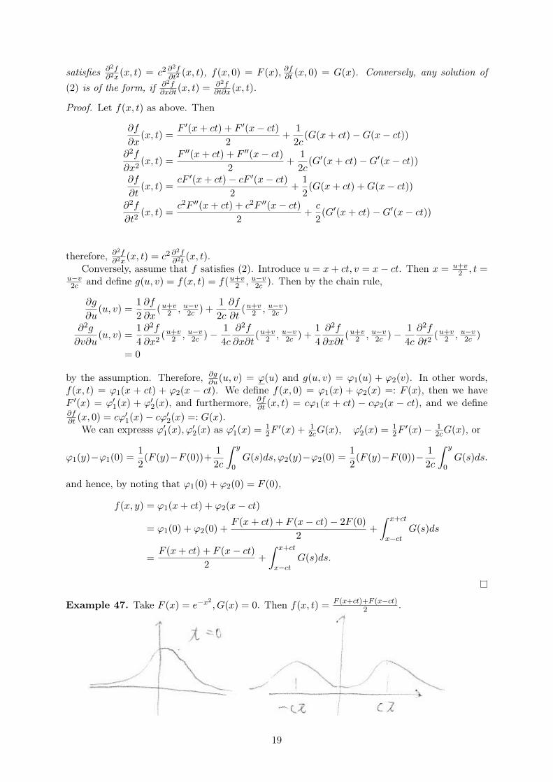
Example 47. Take F (x) = e−x2, G(x) = 0. Then f(x, t) = F (x+ct)+F (x−ct)
2 .
19
Oct 21. Implicit functions and partial derivatives
Recall that a function or a scalar field f(·) defined on a subset S of Rn assigns to each pointx ∈ S a real number f(x), and it is represented by a curve or a surface.
Example 48. Explicitly given functions.
• f(x) = x2
• f(x, y) = cosxey
• f(x, y, z) = e198x7z + (x− 2345)32 + (x2 + 28)(y3 − 2π)...
Sometime a function is defined implicitly: consider the equation
x2 + y2 = 1.
This defines a circle. By solving this equation, we obtain
y = ±√
1− x2.
Namely, the curve x2+y2 = 0 defines implicitly the function y = f(x) = ±√
1− x2. Similarly,the equation x2 + y2 + z2 = 1 represents a sphere. It defines the function (scalar field) z =f(x, y) = ±
√1− x2 − y2.
In general, if F (x, y, z) is a function, the equation F (x, y, z) = 0 may define a function (butnot always). Furthermore, even if it defines a function, it is not always possible to solve itexplicitly. Can you solve the following equation in z?
F (x, y, z) = y2 + xz + z2 − ez − 4 = 0
We assume that there is a function f(x, y) such that F (x, y, f(x, y)) = 0. Even if we donot know the explicit form of f(x, y), we can obtain some information about ∂f
∂x ,∂f∂y .
Consider g(x, y) = F (x, y, f(x, y)) = 0 as a function of two variables x, y. Obviously we have∂g∂x = ∂g
∂y = 0. On the other hand, one can see it as
g(x, y) = F (u1(x, y), u2(x, y), u3(x, y)) with u1(x, y) = x, u2(x, y) = y, u3(x, y) = f(x, y).
By the chain rule,
0 =∂g
∂x(x, y) =
∂F
∂x(x, y, f(x, y)) · 1 +
∂F
∂y(x, y, f(x, y)) · 0 +
∂F
∂z(x, y, f(x, y)) · ∂f
∂x(x, y),
therefore,∂f
∂x(x, y) = −
∂F∂x (x, y, f(x, y))∂F∂z (x, y, f(x, y))
.
Similarly,∂f
∂y(x, y) = −
∂F∂y (x, y, f(x, y))
∂F∂z (x, y, f(x, y))
.
Note that F (x, y, z) is explicitly given.
Example 49. F (x, y, z) = y2 + xz + z2 − ez − C, where C ∈ R. Assume the existence off(x, y) such that F (x, y, f(x, y)) = 0. Find the value of C such that f(0, e) = 2 and compute∂f∂x (0, e), ∂f∂y (0, e).Solution. F (0, e, f(0, e)) = F (0, e, 2) = e2 + 0 + 22 − e2 − C = 0 =⇒ C = 4. Note that
• ∂F∂x (x, y, z) = z and hence ∂F
∂x (x, y, f(x, y)) = f(x, y)
20
• ∂F∂y (x, y, z) = 2y and hence ∂F
∂y (x, y, f(x, y)) = 2y
• ∂F∂z (x, y, z) = x+ 2z − ez and hence ∂F
∂z (x, y, f(x, y)) = x+ f(x, y)− ef(x,y)
Therefore,
∂f
∂x(x, y) = −
∂F∂x (x, y, f(x, y))∂F∂z (x, y, f(x, y))
= − f(x, y)
x+ 2f(x, y)− ef(x,y)
∂f
∂x(0, e) = − f(0, e)
0 + 2f(0, e)− ef(0,e)=
2
e2 − 4.
∂f
∂y(x, y) = −
∂F∂y (x, y, f(x, y))
∂F∂z (x, y, f(x, y))
= − 2y
x+ 2f(x, y)− ef(x,y)
∂f
∂y(0, e) = − 2e
0 + 2f(0, e)− ef(0,e)=
2e
e2 − 4.
More generally, if F (x1, · · · , xn) = 0 defines a function xn = f(x1, · · · , xn−1), then
∂f
∂xk(x1, · · · , xn−1) = −
∂F∂xk
(x1, · · · , xn−1, f(x1, · · · , xn−1))∂F∂xn
(x1, · · · , xn−1, f(x1, · · · , xn−1)).
Next, let us consider two surfaces F (x, y, z) = 0 and G(x, y, z) = 0 and assume that theirintersection is a curve (X(z), Y (z), z). Namely, F (X(z), Y (z), z) = 0, G(X(z), Y (z), z) = 0.
Example 50. The unit sphere F (x, y, z) = x2 +y2 + z2 = 0 and the xz-plane G(x, y, z) = y = 0has the intersection x2 + z2 = 0 =⇒ x = X(z) = ±
√1− z2, Y (z) = 0.
Even if X(z) and Y (z) are only implicitly given, we can compute their derivatives. Asbefore, put f(z) = F (X(z), Y (z), z) = 0, g(z) = G(X(z), Y (z), z) = 0. By the chain rule,
0 = f ′(z) = X ′(z)∂F
∂x(X(z), Y (z), z) + Y ′(z)
∂F
∂x(X(z), Y (z), z) +
∂F
∂z(X(z), Y (z), z).
Similarly,
0 = g′(z) = X ′(z)∂G
∂x(X(z), Y (z), z) + Y ′(z)
∂G
∂x(X(z), Y (z), z) +
∂G
∂z(X(z), Y (z), z).
From these, we obtain(X ′(z)Y ′(z)
)=
(∂F∂x
∂F∂y
∂G∂x
∂G∂y
)−1(X(z), Y (z), z) ·
(−∂G∂z
−∂G∂z
)(X(z), Y (z), z).
Example 51. Computations of partial derivatives.
• x = u+ v, y = uv2 defines u(x, y), v(x, y). Compute ∂v∂x .
Solution. By eliminating u, we obtain xv2 − v3 − y = 0. In other words, F (x, y, v) = 0where F (x, y, v) = xv2 − v3 − y. By the formula above, with ∂F
∂x = v2, ∂F∂v = 2xv − 3v2,∂v∂x = − v(x,v)2
2xv(x,y)−3v(x,y)2 .
• Assume that g(x, y) = 0 defines implicitly Y (x). Let f(x, y) be another function. Thenh(x) = f(x, Y (x)) is a function of x. By the chain rule,
h′(x) =∂f
∂x(x, Y (x)) +
∂f
∂y(x, Y (x))Y ′(x)
=∂f
∂x(x, Y (x))−
∂g∂x(x, Y (x))∂g∂y (x, Y (x))
∂f
∂y(x, Y (x))
21
• Let u be defined by F (u+x, yu) = u. Let u = g(x, y), then g(x, y) = F (g(x, y)+x, yg(x, y)),and
∂g
∂x(x, y)
=∂F
∂X(g(x, y) + x, yg(x, y))
(∂g
∂x(x, y) + 1
)+∂F
∂Y(g(x, y) + x, yg(x, y)) · y ∂g
∂x(x, y)
=⇒ ∂g
∂x(x, y) =
− ∂F∂X (g(x, y) + x, yg(x, y))
∂F∂Y (g(x, y) + x, yg(x, y)) + y ∂F∂X (g(x, y) + x, yg(x, y))− 1
• 2x = v2 − u2, y = uv defines implicitly u(x, y), v(x, y) (it is also possible to solve them:2x+ (yv )2 = v2, ( yu)2 − u2 = 2x). Compute ∂u
∂x ,∂u∂y ,
∂v∂x ,
∂v∂y .
Solution. By differentiating with respect to x,
2 = 2v∂v
∂x− 2u
∂u
∂x, 0 =
∂u
∂xv + u
∂v
∂x
From which one obtains
∂u
∂x= − u
u2 + v2,
∂v
∂x=
v
u2 + v2.
Similarly,∂u
∂y=
v
u2 + v2,
∂v
∂y=
u
u2 + v2.
Oct 23. Minima, maxima and saddle points
Various extremal points
Let S ⊂ Rn be an open set, f : S → R be a scalar field and aaa ∈ S. Recall that B(aaa, r) = {xxx ∈Rn : ‖xxx− aaa‖ < r} is the r-ball centered at aaa.
Definition 52. (Minima and maxima)
• If f(aaa) ≤ f(xxx) (respectively f(aaa) ≥ f(xxx)) for all xxx ∈ S, then f(aaa) is said to be the absoluteminimum (resp. maximum) of f .
• If f(aaa) ≤ f(xxx) (respectively f(aaa) ≥ f(xxx)) for xxx ∈ B(aaa, r) for some r, then f(aaa) is said tobe a relative minimum (resp. maximum)
Theorem 53. If f is differentiable and has a relative minumum (resp. maximum) at aaa, then∇f(aaa) = 0.
Proof. We prove the statement only for a relative minumum, because the other case is analogous.For any unit vector yyy, consider g(u) = f(aaa + uyyy). As aaa is a relative minumum, g has a relativeminumum at u = 0, therefore, g′(0) = 0, and f ′(aaa;yyy) = 0 for any yyy. This implies that ∇f(aaa) =000.
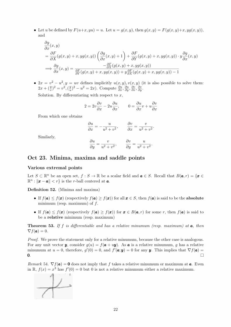
Remark 54. ∇f(aaa) = 000 does not imply that f takes a relative minumum or maximum at aaa. Evenin R, f(x) = x3 has f ′(0) = 0 but 0 is not a relative minumum either a relative maximum.
22
Definition 55. (Stationary points)
• If ∇f(aaa) = 000, then aaa is called a stationary point.
• If ∇f(aaa) = 000 and aaa is neither a relative minumum nor a relative maximum, then aaa is calleda suddle point.
Example 56. (Stationary points)
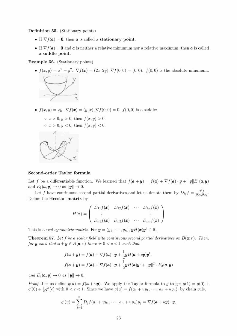
• f(x, y) = x2 + y2. ∇f(xxx) = (2x, 2y),∇f(0, 0) = (0, 0). f(0, 0) is the absolute minumum.
• f(x, y) = xy. ∇f(xxx) = (y, x),∇f(0, 0) = 0. f(0, 0) is a saddle:
◦ x > 0, y > 0, then f(x, y) > 0.◦ x > 0, y < 0, then f(x, y) < 0.
Second-order Taylor formula
Let f be a differentiable function. We learned that f(aaa + yyy) = f(aaa) +∇f(aaa) · yyy + ‖yyy‖E1(aaa,yyy)and E1(aaa,yyy)→ 0 as ‖yyy‖ → 0.
Let f have continuous second partial derivatives and let us denote them by Dijf = ∂2f∂xi,∂xj
.Define the Hessian matrix by
H(xxx) =
D11f(xxx) D12f(xxx) · · · D1nf(xxx)...
...Dn1f(xxx) Dn2f(xxx) · · · Dnnf(xxx)
This is a real symmetric matrix. For yyy = (y1, · · · , yn), yyyH(xxx)yyyt ∈ R.
Theorem 57. Let f be a scalar field with continuous second partial derivatives on B(aaa; r). Then,for yyy such that aaa+ yyy ∈ B(aaa; r) there is 0 < c < 1 such that
f(aaa+ yyy) = f(aaa) +∇f(aaa) · yyy +1
2yyyH(aaa+ cyyy)yyyt,
f(aaa+ yyy) = f(aaa) +∇f(aaa) · yyy +1
2yyyH(aaa)yyyt + ‖yyy‖2 · E2(aaa,yyy)
and E2(aaa,yyy)→ 0 as ‖yyy‖ → 0.
Proof. Let us define g(u) = f(aaa + uyyy). We apply the Taylor formula to g to get g(1) = g(0) +g′(0) + 1
2g′′(c) with 0 < c < 1. Since we have g(u) = f(a1 + uy1, · · · , an + uyn), by chain rule,
g′(u) =n∑j=1
Djf(a1 + uy1, · · · , an + uyn)yj = ∇f(aaa+ uyyy) · yyy,
23
where Djf = ∂f∂xj
. Similarly,
g′′(u) =
n∑i,j=1
Dijf(a1 + uy1, · · · , an + uyn)yiyj = yyyH(aaa+ uyyy)yyyt,
from which the first equation follows. As for the second equation, we define E2 by E2(aaa,yyy) =12(yyyH(aaa+ cyyy)−H(aaa)t)yyyt/‖yyy‖2. Then
|E2(aaa,yyy)| ≤ 1
2
n∑i,j=1
|yiyj |‖yyy‖2
|Dijf(aaa+ cyyy)−Dijf(aaa)| → 0
as ‖y‖ → 0, by the continuity of Dijf(aaa).
Classifiying stationary points
We give a criterion to deterine whether aaa is a minumum/maximum/saddle when ∇f(aaa) = 000.
Theorem 58. Let A =
a11 · · · a1n...
...an1 · · · ann
be a real symmetric matrix, and Q(yyy) = yyyAyyyt.
Then,
• Q(yyy) > 0 for all yyy 6= 000 if and only if all eigenvalues of A are positive.
• Q(yyy) < 0 for all yyy 6= 000 if and only if all eigenvalues of A are negative.
Proof. A real symmetric matrix A can be diagonalized by an orthogonal matrix C, namely,
L = CtAC =
λ1 0 · · · 00 λ2 · · · 0...
. . ....
0 0 · · · λn
. If all λj > 0, then Q(yyy) = yyyCCtACCtyyyt = vvvLvvvt =
∑j λjvj > 0, where vvv = yyyC. If Q(yyy) > 0 for all yyy 6= 000, then especially for yyyk = uuukC where
uuuk = (0, · · · , 0, 1k-th
, 0, · · · , 0), and Q(yyyk) = λk > 0.
Theorem 59. Let f be a scalar field with continuous second derivatives on B(aaa; r). Assume that∇f(aaa) = 000. Then,
(a) If all the eigenvalues λj of H(aaa) are positive, then f has a relative minumum at aaa.
(b) If all the eigenvalues λj of H(aaa) are negative, then f has a relative maximum at aaa.
(c) If some λk > 0 and λ` <, then aaa is a saddle.
Proof. (a) Let Q(yyy) = yyyH(aaa)yyyt. Let h be te smallest eigenvalue of H(aaa), h > 0 and diagonalizeh(aaa) by C. We set yyyC = vvv, then ‖yyy‖ = ‖vvv‖. Furthermore,
yyyH(aaa)yyyt = vvvCH(aaa)Ctvvvt =∑j
λjv2j > h
∑j
v2j = h‖vvv‖2 = h‖yyy‖2.
By Theorem 57,f(aaa+ yyy) = f(aaa) + yyyH(aaa)yyyt + ‖yyy‖2E2(aaa,yyy).
As H2(aaa,yyy)→ 0 as ‖yyy‖ → 0, there is r1 such that if ‖yyy‖ < r1, then |E2(aaa,yyy)| < h2 . Now
f(aaa+ yyy) = f(aaa) +1
2yyyH(aaa)yyyt + ‖yyy‖2E2(aaa,yyy) > f(aaa) +
h
2‖yyy‖2 − h
2‖yyy‖ > f(aaa),
24
hence f has a relative minumum at aaa.(b) This case is similar as above.(c) Let yyyk be an eigenvector with eigenvalue λk, yyy` be an eigenvector with eigenvalue λ`. As
in (a), f(aaa+ cyyyk) > f(aaa) and as in (b) f(aaa+ cyyy`) < f(aaa) for small c, hence aaa is a saddle.
Example 60. f(x, y) = xy. λϕ(x, y) = (y, x), H(x, y) =
(0 11 0
)(0, 0) is a stationary point
and H(0, 0) has eigenvalues 1,−1, hence (0, 0) is a saddle.
25


