
8/3/2019 Marco Baldi et al- Hydrodynamical N-body simulations of coupled dark energy cosmologies
http://slidepdf.com/reader/full/marco-baldi-et-al-hydrodynamical-n-body-simulations-of-coupled-dark-energy 1/21
a r X i v : 0 8 1 2
. 3 9 0 1 v 2
[ a s t r o - p h ]
5 F e b 2 0 1 0
Mon. Not. R. Astron. Soc. 000, 1–21 (2008) Printed 5 February 2010 (MN LATEX style file v2.2)
Hydrodynamical N-body simulations of coupled dark energy
cosmologies
Marco Baldi1, Valeria Pettorino2, Georg Robbers2, Volker Springel11 Max-Planck-Institut f¨ ur Astrophysik, Karl-Schwarzschild Strasse 1, D-85748 Garching, Germany.2 Institut f ¨ ur Theoretische Physik, Universit¨ at Heidelberg, P hilosophenweg 16, D-69120 Heidelberg, Germany.
5 February 2010
ABSTRACT
If the accelerated expansion of the Universe at the present epoch is driven by a dark en-ergy scalar field, there may well be a non-trivial coupling between the dark energy and the colddark matter (CDM) fluid. Such interactions give rise to new features in cosmological structure
growth, like an additional long-range attractive force between CDM particles, or variations of the dark matter particle mass with time. We have implemented these effects in the N-bodycode GADGET-2 and present results of a series of high-resolution N-body simulations wherethe dark energy component is directly interacting with the cold dark matter. As a consequenceof the new physics, CDM and baryon distributions evolve differently both in the linear andin the nonlinear regime of structure formation. Already on large scales a linear bias developsbetween these two components, which is further enhanced by the nonlinear evolution. We alsofind, in contrast with previous work, that the density profiles of CDM halos are less concen-trated in coupled dark energy cosmologies compared with ΛCDM, and that this feature doesnot depend on the initial conditions setup, but is a specific consequence of the extra physicsinduced by the coupling. Also, the baryon fraction in halos in the coupled models is signifi-cantly reduced below the universal baryon fraction. These features alleviate tensions betweenobservations and the ΛCDM model on small scales. Our methodology is ideally suited to ex-plore the predictions of coupled dark energy models in the fully non-linear regime, which can
provide powerful constraints for the viable parameter space of such scenarios.Key words: dark energy – dark matter – cosmology: theory – galaxies: formation
1 INTRODUCTION
The last decade has seen an astonishing amount of new cosmo-
logical data from many different experiments, ranging from large-
scale structure surveys (Percival et al. 2001, e.g.) to Cosmic Mi-
crowave Background (CMB) (Komatsu et al. 2008) and Type Ia
Supernovae (Riess et al. 1998; Perlmutter et al. 1999; Astier et al.
2006) observations. These experiments all consistently show that
the Universe is almost spatially flat with a current expansion rate of about 70kms−1Mpc−1, and contains a total amount of matter that
accounts for only∼ 24% of the total energy density. From a theore-
tical point of view, understanding the remaining 76% – which must
be in the form of some dark energy (DE) component able to drive
an accelerated expansion – is a serious challenge.
A simple cosmological constant would be in agreement with
a large number of observational datasets, but would also raise two
fundamental questions concerning its fine-tuned value and the co-
incidence of its domination over cold dark matter (CDM) only at
a relatively recent cosmological epoch. An alternative consists of
identifying the dark energy component with a dynamic scalar field
(Wetterich 1988; Ratra & Peebles 1988), thereby seeking an expla-
nation of the fundamental problems challenging the cosmological
constant in the properties of the dynamic evolution of such scalar
field.
An interesting suggestion recently developed concerns the in-
vestigation of possible interactions between the dark energy scalar
field and other matter species in the Universe (Wetterich 1995;
Amendola 2000; Farrar & Peebles 2004; Gubser & Peebles 2004;
Farrar & Rosen 2007). The existence of such a coupling could pro-
vide a unique handle for a deeper understanding of the DE problem(Quartin et al. 2008; Brookfield et al. 2008; Gromov et al. 2004;
Mangano et al. 2003; Anderson & Carroll 1997). It is then cru-
cial to understand in detail what effects such a coupling imprints
on observable features like, for example, the CMB and structure
formation (La Vacca et al. 2009; Bean et al. 2008; Bertolami et al.
2007; Matarrese et al. 2003; Wang et al. 2007; Guo et al. 2007;
Mainini & Bonometto 2007a; Lee et al. 2006).
In this paper, we perform the first fully self-consistent high-
resolution hydrodynamic N-body simulations of cosmic structure
formation for a selected family of coupled DE cosmologies. The
interaction between DE and CDM is expected to imprint characte-
ristic features in linear and nonlinear structures, and could possi-
c 2008 RAS

8/3/2019 Marco Baldi et al- Hydrodynamical N-body simulations of coupled dark energy cosmologies
http://slidepdf.com/reader/full/marco-baldi-et-al-hydrodynamical-n-body-simulations-of-coupled-dark-energy 2/21
2 M. Baldi, V. Pettorino, G. Robbers, V. Springel
bly open up new ways to overcome a series of observational chal-
lenges for the ΛCDM concordance cosmology, ranging from the
satellite abundance in CDM halos (Navarro et al. 1996), to the ob-
served low baryon fraction in large galaxy clusters (Allen et al.
2004; Vikhlinin et al. 2006; LaRoque et al. 2006), and to the so-
called “cusp-core” problem for the density profiles of CDM halos,
that was first raised in relation to observations of dwarf and low-
surface-brightness galaxies (Moore 1994; Flores & Primack 1994;Simon et al. 2003), but that more recent studies seem to extend to
a wider range of objects including Milky-Way type spiral galaxies
(Navarro & Steinmetz 2000; Binney & Evans 2001) up to galaxy
groups and clusters (Sand et al. 2002, 2004; Newman et al. 2009).
In the following we will consider DE as the energy associated
with a scalar field φ (Wetterich 1988; Ratra & Peebles 1988) whose
energy density and pressure are defined respectively as the (0, 0)and (0, i) components of its stress energy tensor, so that1:
ρφ ≡1
2
φ′2
a2+ U (φ) , (1)
pφ ≡1
2
φ′2
a2− U (φ) , (2)
with U (φ) being the self interaction potential. The models we in-vestigate in this work by means of detailed high-resolution N-body
simulations are physically identical to the ones already studied by
Maccio et al. (2004). With respect to this previous work, however,
our analysis significantly improves on the statistics of the number
of cosmic structures analyzed in each of our different cosmologi-
cal models and on the dynamic range of the simulations. We also
extend the analysis to a wider range of observable effects arising
from the new physics of the DE-CDM interaction, and we include
hydrodynamics. Despite the physical models investigated be iden-
tical, our outcomes are starkly different from the ones found in
Maccio et al. (2004).
This work is organized as follows. In Section 2 we detail the
coupled DE cosmologies under investigation, both regarding the
background evolution and the perturbations, and we introduce a
numerical package to integrate the full set of background and per-
turbation equations up to linear order. In Section 3, we describe the
numerical methods we use, and the particular set of simulations we
have run. We then present and discuss our results for N-body sim-
ulations for a series of coupled DE models in Section 4. Finally, in
Section 5 we draw our conclusions.
2 COUPLED DARK ENERGY COSMOLOGIES
Coupled cosmologies can be described following the considera-
tion (Kodama & Sasaki 1984) that in any multicomponent system,
though the total stress energy tensor T µν is conservedα
∇νT ν(α)µ = 0 , (3)
the T µν(α) for each species α is, in general, not conserved and
its divergence has a source term Q(α)µ representing the possibility
that species are coupled:
∇νT ν(α)µ = Q(α)µ , (4)
1 In this work we always denote with a prime the derivative with respect
to the conformal time τ , and with an overdot the derivative with respect
to the cosmic time t. The two time variables are related via the equation:
dτ = dt/a.
with the constraintα
Q(α)µ = 0 . (5)
Furthermore, we will assume a flat Friedmann-Robertson-Walker
(FRW) cosmology, in which the line element can be written as
ds2 = a2(τ )(−dτ 2 + δijdxidxj) where a(τ ) is the scale factor.
2.1 Background
The Lagrangian of the system is of the form:
L = −1
2∂ µφ∂ µφ− U (φ)−m(φ)ψψ + Lkin[ψ] , (6)
in which the mass of matter fields ψ coupled to the DE is a function
of the scalar field φ. In the following we will consider the case in
which the DE is only coupled to cold dark matter (CDM, hereafter
denoted with a subscript c). The choice m(φ) specifies the coupling
and as a consequence the source term Q(φ)µ via the expression:
Q(φ)µ =∂ ln m(φ)
∂φρc ∂ µφ. (7)
Due to the constraint (5), if no other species is involved in the cou-pling, Q(c)µ = −Q(φ)µ.
The zero-component of equation (4) provides the conservation
equations for the energy densities of each species:
ρ′φ = −3Hρφ(1 + wφ)−Q(φ)0 , (8)
ρ′c = −3Hρc + Q(φ)0 .
Here we have treated each component as a fluid with T ν(α)µ =(ρα + pα)uµuν + pαδνµ, where uµ = (−a, 0, 0, 0) is the fluid 4-
velocity and wα ≡ pα/ρα is the equation of state. The class of
models considered here corresponds to the choice:
m(φ) = m0e−β(φ)φM , (9)
with the coupling term equal to
Q(φ)0 = −β(φ)
M ρcφ′ . (10)
This set of cosmologies has been widely investigated, for β(φ)given by a constant, both in its background and linear perturba-
tion features (Wetterich 1995; Amendola 2000) as well as with
regard to the effects on structure formation (Amendola 2004;
Pettorino & Baccigalupi 2008) , and via a first N-body simulation
(Maccio et al. 2004).
2.2 Linear perturbations
We now perturb the quantities involved in our cosmological frame-
work up to the first order in the perturbations ( Kodama & Sasaki1984; Ma & Bertschinger 1995). The perturbed metric tensor can
then be written as
gµν(τ, x) = gµν(τ ) + δgµν(τ, x) , (11)
where δgµν ≪ 1 is the linear metric perturbation, whose expres-
sion in Fourier space is given by:
δg00 = −2a2A Y , δ g0i = −a2BY i ,
δgij = 2a2[H LY δij + H T Y ij] , (12)
where A,B,H L, H T are functions of time and of the wave vec-
tor k, and Y i, Y ij are the vector and tensor harmonic functions ob-
tained by deriving Y, defined as the solution of the Laplace equation
c 2008 RAS, MNRAS 000, 1–21

8/3/2019 Marco Baldi et al- Hydrodynamical N-body simulations of coupled dark energy cosmologies
http://slidepdf.com/reader/full/marco-baldi-et-al-hydrodynamical-n-body-simulations-of-coupled-dark-energy 3/21
Hydrodynamical N-body simulations of coupled dark energy cosmologies 3
δij∇i∇jY = −|k|2Y . Analogously, the perturbed stress energy
tensor for each fluid (α) can be written as T µ(α)ν
= T µ(α)ν
+ δT µ(α)ν
where the perturbations read as:
δT 0(α)0 = −ρ(α)δ(α)Y , (13)
δT 0(α)i = h(α)(v(α) −B)Y i ,
δT i(α)0 = −h(α)v(α)Y i ,
δT i(α)j = p(α)
πL(α)Y δij + πT (α)Y ij
.
The perturbed conservation equations then become:
(ραδα)′+3Hραδα+hα(kvα+3H ′L)+3H pαπLα = −δQ(α)0(14)
for the energy density perturbation δα = δρα/ρα, and:
[hα(vα −B)]′ + 4Hhα(vα −B)
−kpαπLα − hαkA +2
3kpπTα = δQ(α)i (15)
for the velocity perturbation vα.
The scalar field φ can also be perturbed, yielding in Fourier
space
φ = φ + δφ = φ + χ(τ )Y . (16)
Furthermore, we can express the perturbations of the source as:
δQ(φ)0 = −β(φ)
M ρcδφ′ −
β(φ)
M φ′δρc −
β,φM
φ′ρcδφ , (17)
δQ(φ)i = kβ(φ)
M ρcδφ . (18)
In the Newtonian gauge (B = 0, H T = 0, H L = Φ, A = Ψ) the
set of equations for the density and velocity perturbations for DE
and CDM read:
δρ′φ + 3H(δρφ + δpφ) + khφvφ + 3hφΦ′ = (19)
β(φ)M
ρcδφ′ + β(φ)M
φ′δρc + β,φM
φ′δφρc ,
δρ′c + 3Hδρc + kρcvc + 3ρcΦ′ =
−β(φ)
M ρcδφ′ −
β(φ)
M φ′δρc −
β,φM
φ′δφρc ,
hφv′φ +
h′φ + 4Hhφ
vφ − kδpφ − khφΨ = kβ(φ)
M ρcδφ ,
v′c +
H−
β(φ)
M φ′
vc − kΨ = −kβ(φ)
M δφ .
The perturbed Klein Gordon equation in Newtonian gauge reads:
δφ′′ + 2Hδφ′ +
k2 + a2U ,φφ
δφ − φ′
Ψ′ − 3Φ′
+
2a2U ,φΨ = 3H2Ωc [β(φ)δc + 2β(φ)Ψ+ β,φ(φ)δφ] .(20)
For the N-body implementation we are interested in, the New-
tonian limit holds, for which λ ≡ H/k ≪ 1. In this case we have
δφ ∼ 3λ2Ωcβ(φ)δc . (21)
In this limit, the gravitational potential is approximately given by
Φ ∼3
2
λ2
M 2
α=φ
Ωαδα . (22)
We can then define an effective gravitational potential
Φc ≡ Φ+β(φ)
M δφ, (23)
which also reads, in real space and after substituting the expressions
for Φ (Eqn. 22) and for δφ (Eqn. 21):
∇2Φc = −
a2
2ρcδc
1 + 2β2(φ)
−
a2
2
α=φ,c
ραδα , (24)
where the last term takes into account the case in which other com-
ponents not coupled to the DE are present in the total energy budget
of the Universe. Cold dark matter then feels an effective gravita-
tional constant
Gc = GN [1 + 2β2(φ)], (25)
where GN is the usual Newtonian value. Therefore, the strength
of the gravitational interaction is not a constant anymore if β is a
function of the scalar field φ. The last equation in (19), written in
real space and in terms of the effective gravitational potential, gives
a modified Euler equation of the form:
∇v′c +
H−
β(φ)
M φ′∇vc +
3
2H2 Ωcδc + 2Ωcδcβ2(φ) +
α=φ,c
Ωαδα = 0 . (26)
As in Amendola (2004), if we assume that the CDM is con-
centrated in one particle of mass mc at a distance r from a particle
of mass M c at the origin, we can rewrite the CDM density contri-
bution as
Ωcδc =8πGM ce
−
β(φ)dφ
δ(0)
3H2a, (27)
where we have used the fact that a non-relativistic particle at po-
sition r has a density given by mcnδ(r) (where δ(r) stands for
the Dirac distribution) with mass given by mc ∝ e−
β(φ)dφ
, for-
mally obtained from equation (9). We have further assumed that the
density of the M c mass particle is much larger than ρc. The Euler
equation in cosmic time (dt = a dτ ) can then be rewritten in the
form of an acceleration equation for the particle at position r:
vc = −H vc −∇GcM c
r, (28)
where we explicitely see that the usual equation is modified in three
ways.
First, the velocity-dependent term now contains an additional
contribution given by the second term of the expression defining
H :
H ≡ H
1−
β(φ)
M
φ
H
. (29)
Second, the CDM particles feel an effective gravitational constant
G given by (25). Third, the CDM particles have an effective mass,
varying with time, given by:
M c ≡ M ce−
β(φ)dφ
dada
. (30)
Eqn. 28 is very important for our discussion since it represents the
starting point for the implementation of coupled DE models in an
N-body code. We will discuss in detail how this implementation is
realized in Sec. 3.1, but it is important to stress here that Eqn. 28
is written in a form that explicitely highlights its vectorial nature,
which has not been presented in previous literature. The vectorial
nature of Eqn. 28 is a key point in its numerical implementation
and therefore needs to be properly taken into account.
c 2008 RAS, MNRAS 000, 1–21
8/3/2019 Marco Baldi et al- Hydrodynamical N-body simulations of coupled dark energy cosmologies
http://slidepdf.com/reader/full/marco-baldi-et-al-hydrodynamical-n-body-simulations-of-coupled-dark-energy 4/21
4 M. Baldi, V. Pettorino, G. Robbers, V. Springel
In the N-body analysis carried out in the present paper, we
consider β to be a constant, so that the effective mass formally reads
M c ≡ M ce−β(φ−φ0). We defer an investigation of variable β(φ) to
future work. We have numerically solved the full background and
linear perturbation equations with a suitably modified version of
CMBEASY (Doran 2005), briefly described in the following section.
2.3 Background and linear perturbation integration of
coupled DE models: a modified CMBEASY package
We have implemented the full background and linear perturbation
equations derived in the previous section in the Boltzmann code
CMBEASY (Doran 2005) for the general case of a DE component
coupled to dark matter via a coupling term given by Eqn. ( 4). The
form of this coupling, as well as the evolution of the DE (either
modelled as a scalar field or purely as a DE fluid), can be freely
specified in our implementation.
Compared to the standard case of uncoupled DE, the modifi-
cations include a modified behaviour of the background evolution
of CDM and DE given by Eqs. (8) and (9), as well as the implemen-
tation of the linear perturbations described by Eqn. (19), and their
corresponding adiabatic initial conditions. The presence of a CDM-
DE coupling furthermore complicates the choice of suitable initial
conditions even for the background quantities, since dark matter
no longer scales as a−3, and so cannot simply be rescaled from its
desired value today. For each of the models considered here, we
choose to set the initial value of the scalar field close to its tracker
value in the uncoupled case, and then adjust the value of the poten-
tial constant Λ (see Eqn. (31) below) and the initial CDM energy
density such that we obtain the desired present-day values.
3 THE SIMULATIONS
The aim of this work is to investigate the effects that a couplingbetween DE and other cosmological components, as introduced in
Sec. 2, can have on cosmic structure formation, with a particular
focus on the nonlinear regime which is not readily accessible by
the linear analytic approach described in Sec. 2.2. To this end we
study a set of cosmological N-body simulations performed with the
code GADGET-2 (Springel 2005), that we suitably modified for this
purpose.
The required modifications of the standard algorithms of
the N-body code for simulating coupled DE cosmologies are
extensively described in Sec. 3.1. Interestingly, they require to
reconsider and in part drop several assumptions and approx-
imations that are usually adopted in N-body simulations. We
note that previous attempts to use cosmological N-body simula-
tions for different flavours of modified Newtonian gravity havebeen discussed, for example, in Maccio et al. (2004); Nusser et al.
(2005); Stabenau & Jain (2006); Kesden & Kamionkowski (2006);
Springel & Farrar (2007); Laszlo & Bean (2008); Sutter & Ricker
(2008); Oyaizu (2008); Keselman et al. (2009) but to our knowl-
edge Maccio et al. (2004) is the only work to date focusing
on the properties of nonlinear structures in models of coupled
quintessence.
Therefore, with our modified version of GADGET-2 we first
ran a set of low-resolution cosmological simulations (Lbox =320h−1Mpc, N part = 2× 1283) for the same coupled DE models
investigated in Maccio et al. (2004), but with cosmological parame-
ters updated to the latest results from WMAP (Komatsu et al. 2008)
Parameter Value
ΩCDM 0.213
H 0 71.9 km s−1 Mpc−1
ΩDE 0.743
σ8 0.769
Ωb 0.044
n 0.963
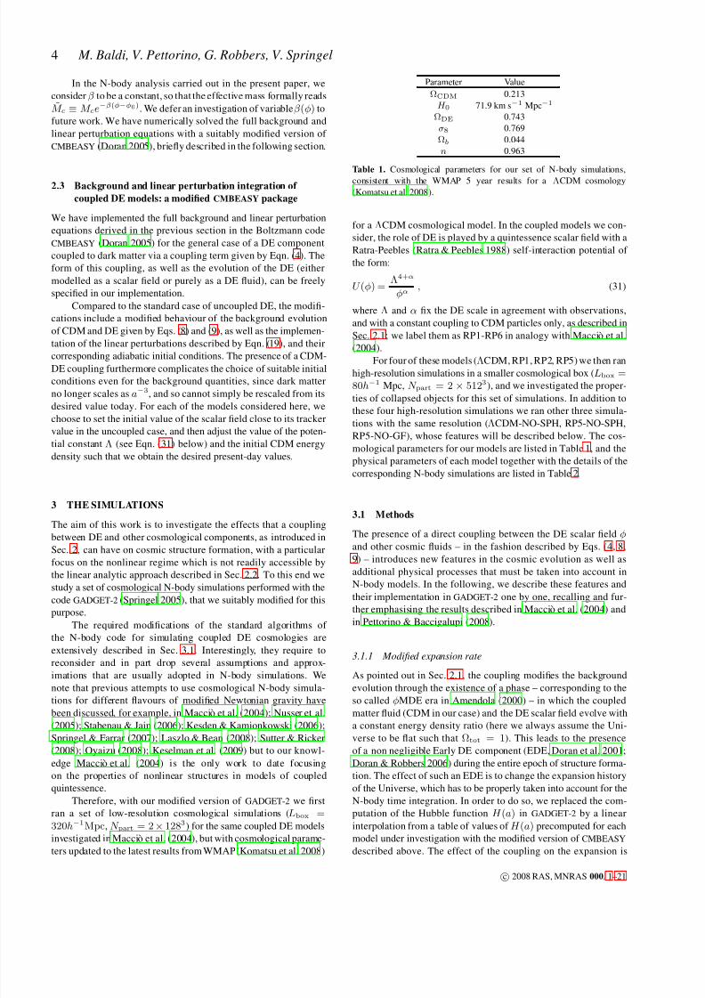
Table 1. Cosmological parameters for our set of N-body simulations,
consistent with the WMAP 5 year results for a ΛCDM cosmology
(Komatsu et al. 2008).
for a ΛCDM cosmological model. In the coupled models we con-
sider, the role of DE is played by a quintessence scalar field with a
Ratra-Peebles (Ratra & Peebles 1988) self-interaction potential of
the form:
U (φ) =Λ4+α
φα, (31)
where Λ and α fix the DE scale in agreement with observations,
and with a constant coupling to CDM particles only, as described in
Sec. 2.1; we label them as RP1-RP6 in analogy with Maccio et al.
(2004).For four of these models (ΛCDM, RP1, RP2, RP5) we then ran
high-resolution simulations in a smaller cosmological box (Lbox =80h−1 Mpc, N part = 2 × 5123), and we investigated the proper-
ties of collapsed objects for this set of simulations. In addition to
these four high-resolution simulations we ran other three simula-
tions with the same resolution (ΛCDM-NO-SPH, RP5-NO-SPH,
RP5-NO-GF), whose features will be described below. The cos-
mological parameters for our models are listed in Table 1, and the
physical parameters of each model together with the details of the
corresponding N-body simulations are listed in Table 2.
3.1 Methods
The presence of a direct coupling between the DE scalar field φand other cosmic fluids – in the fashion described by Eqs. (4, 8,
9) – introduces new features in the cosmic evolution as well as
additional physical processes that must be taken into account in
N-body models. In the following, we describe these features and
their implementation in GADGET-2 one by one, recalling and fur-
ther emphasising the results described in Maccio et al. (2004) and
in Pettorino & Baccigalupi (2008).
3.1.1 Modified expansion rate
As pointed out in Sec. 2.1, the coupling modifies the background
evolution through the existence of a phase – corresponding to the
so called φMDE era in Amendola (2000) – in which the coupledmatter fluid (CDM in our case) and the DE scalar field evolve with
a constant energy density ratio (here we always assume the Uni-
verse to be flat such that Ωtot = 1). This leads to the presence
of a non negligible Early DE component (EDE, Doran et al. 2001;
Doran & Robbers 2006) during the entire epoch of structure forma-
tion. The effect of such an EDE is to change the expansion history
of the Universe, which has to be properly taken into account for the
N-body time integration. In order to do so, we replaced the com-
putation of the Hubble function H (a) in GADGET-2 by a linear
interpolation from a table of values of H (a) precomputed for each
model under investigation with the modified version of CMBEASY
described above. The effect of the coupling on the expansion is
c 2008 RAS, MNRAS 000, 1–21
8/3/2019 Marco Baldi et al- Hydrodynamical N-body simulations of coupled dark energy cosmologies
http://slidepdf.com/reader/full/marco-baldi-et-al-hydrodynamical-n-body-simulations-of-coupled-dark-energy 5/21
Hydrodynamical N-body simulations of coupled dark energy cosmologies 5
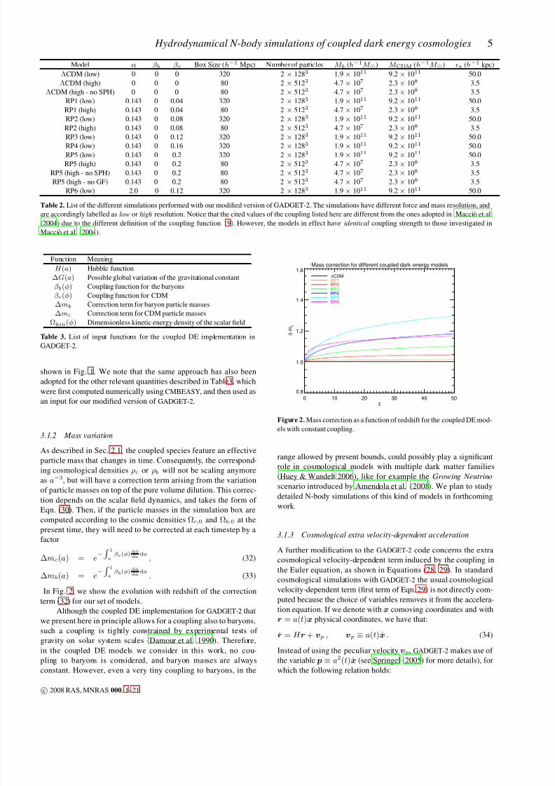
Model α βb βc Box Size (h−1 Mpc) Number of particles M b (h−1M ⊙) M CDM (h−1M ⊙) ǫs (h−1 kpc)
ΛCDM (low) 0 0 0 320 2 × 1283 1.9× 10¹¹ 9.2× 10¹¹ 50.0
ΛCDM (high) 0 0 0 80 2 × 5123 4.7× 10⁷ 2.3× 10⁸ 3.5
ΛCDM (high - no SPH) 0 0 0 80 2 × 5123 4.7× 10⁷ 2.3× 10⁸ 3.5
RP1 (low) 0.143 0 0.04 320 2 × 1283 1.9× 10¹¹ 9.2× 10¹¹ 50.0
RP1 (high) 0.143 0 0.04 80 2 × 5123 4.7× 10⁷ 2.3× 10⁸ 3.5
RP2 (low) 0.143 0 0.08 320 2 × 1283 1.9× 10¹¹ 9.2× 10¹¹ 50.0
RP2 (high) 0.143 0 0.08 80 2 × 5123 4.7× 10⁷ 2.3× 10⁸ 3.5
RP3 (low) 0.143 0 0.12 320 2 × 1283 1.9× 10¹¹ 9.2× 10¹¹ 50.0RP4 (low) 0.143 0 0.16 320 2 × 1283 1.9× 10¹¹ 9.2× 10¹¹ 50.0
RP5 (low) 0.143 0 0.2 320 2 × 1283 1.9× 10¹¹ 9.2× 10¹¹ 50.0
RP5 (high) 0.143 0 0.2 80 2 × 5123 4.7× 10⁷ 2.3× 10⁸ 3.5
RP5 (high - no SPH) 0.143 0 0.2 80 2 × 5123 4.7× 10⁷ 2.3× 10⁸ 3.5
RP5 (high - no GF) 0.143 0 0.2 80 2 × 5123 4.7× 10⁷ 2.3× 10⁸ 3.5
RP6 (low) 2.0 0 0.12 320 2 × 1283 1.9× 10¹¹ 9.2× 10¹¹ 50.0
Table 2. List of the different simulations performed with our modified version of GADGET-2. The simulations have different force and mass resolution, and
are accordingly labelled as low or high resolution. Notice that the cited values of the coupling listed here are different from the ones adopted in Maccio et al.
(2004) due to the different definition of the coupling function (9). However, the models in effect have identical coupling strength to those investigated in
Maccio et al. (2004).
Function Meaning
H (a) Hubble function
∆G(a) Possible global variation of the gravitational constant
βb(φ) Coupling function for the baryons
βc(φ) Coupling function for CDM
∆mb Correction term for baryon particle masses
∆mc Correction term for CDM particle masses
Ωkin(φ) Dimensionless kinetic energy density of the scalar field
Table 3. List of input functions for the coupled DE implementation in
GADGET-2.
shown in Fig. 1. We note that the same approach has also been
adopted for the other relevant quantities described in Table 3, which
were first computed numerically using CMBEASY, and then used as
an input for our modified version of GADGET-2.
3.1.2 Mass variation
As described in Sec. 2.1, the coupled species feature an effective
particle mass that changes in time. Consequently, the correspond-
ing cosmological densities ρc or ρb will not be scaling anymore
as a−3, but will have a correction term arising from the variation
of particle masses on top of the pure volume dilution. This correc-
tion depends on the scalar field dynamics, and takes the form of
Eqn. (30). Then, if the particle masses in the simulation box are
computed according to the cosmic densities Ωc,0 and Ωb,0 at the
present time, they will need to be corrected at each timestep by a
factor
∆mc(a) = e− 1
aβc(φ)dφ
dada
, (32)
∆mb(a) = e−
1
aβb(φ)dφ
dada
. (33)
In Fig. 2, we show the evolution with redshift of the correction
term (32) for our set of models.
Although the coupled DE implementation for GADGET-2 that
we present here in principle allows for a coupling also to baryons,
such a coupling is tightly constrained by experimental tests of
gravity on solar system scales (Damour et al. 1990). Therefore,
in the coupled DE models we consider in this work, no cou-
pling to baryons is considered, and baryon masses are always
constant. However, even a very tiny coupling to baryons, in the
Mass correction for different coupled dark energy models
0 10 20 30 40 50z
0.8
1.0
1.2
1.4
1.6
∆
m c
ΛCDMRP1RP2RP3RP4RP5RP6
Figure 2. Mass correction as a function of redshift for the coupled DE mod-
els with constant coupling.
range allowed by present bounds, could possibly play a significant
role in cosmological models with multiple dark matter families
(Huey & Wandelt 2006), like for example the Growing Neutrino
scenario introduced by Amendola et al. (2008). We plan to study
detailed N-body simulations of this kind of models in forthcoming
work.
3.1.3 Cosmological extra velocity-dependent acceleration
A further modification to the GADGET-2 code concerns the extracosmological velocity-dependent term induced by the coupling in
the Euler equation, as shown in Equations (28, 29). In standard
cosmological simulations with GADGET-2 the usual cosmological
velocity-dependent term (first term of Eqn. 29) is not directly com-
puted because the choice of variables removes it from the accelera-
tion equation. If we denote with x comoving coordinates and with
r = a(t)x physical coordinates, we have that:
r = H r + vp , vp ≡ a(t)x . (34)
Instead of using the peculiar velocity vp, GADGET-2 makes use of
the variable p ≡ a2(t)x (see Springel (2005) for more details), for
which the following relation holds:
c 2008 RAS, MNRAS 000, 1–21

8/3/2019 Marco Baldi et al- Hydrodynamical N-body simulations of coupled dark energy cosmologies
http://slidepdf.com/reader/full/marco-baldi-et-al-hydrodynamical-n-body-simulations-of-coupled-dark-energy 6/21
6 M. Baldi, V. Pettorino, G. Robbers, V. Springel
Hubble functions for different coupled dark energy models
0 20 40 60 80 100z
1•104
2•104
3•104
H
( k m
s - 1
M p c
- 1 )
ΛCDMRP1RP2RP3RP4RP5RP6
Ratio of the Hubble functions to the ΛCDM reference model
0 20 40 60 80 100z
0.9
1.0
1.1
1.2
H / H Λ C D M
ΛCDMRP1RP2RP3RP4RP5RP6
Figure 1. Left panel: Hubble functions as a function of redshift for the different coupled DE models with constant coupling investigated in this work and
described in Table 2 as compared to ΛCDM (black curve). Right panel: Ratio of the Hubble functions of each coupled DE model to the Hubble function for
the reference ΛCDM cosmology as a function of redshift.
vp =1
a ˙ p−H
a p . (35)
It is then straightforward, by using Eqn. (35), to find a generaliza-
tion of Eqn. (28) to a system of N particles, in terms of the new
velocity variable p:
˙ pi =1
a
βγ(φ)
φ
M a pi +
j=i
Gijmjxij
|xij |3
, (36)
where i and j are indices that span over all the particles of the
simulation, γ = c, b for CDM or baryons respectively, and Gij
is the effective gravitational constant between the i-th and the j-
th particles, as determined in Eqn. (25) and whose implementation
will be discussed below.
It is evident from Eqn. (36) that for zero coupling no cosmo-logical velocity-dependent term is present in the acceleration equa-
tion, which is then just Newton’s law in comoving coordinates. In
general, however, whenever a coupling is present, the additional
term
a( ˙ p + ∆ ˙ p) ≡ a ˙ p + βγ(φ)φ
M a pi (37)
has to be explicitely added to the Newtonian acceleration of every
particle. This term does not depend on the matter distribution in the
rest of the Universe. It is therefore a purely cosmological drag that
would be present also in absence of any gravitational attraction. It
is interesting to notice that in the case of constant positive coupling
and a monotonic scalar field potential as investigated here, the ex-
tra cosmological velocity-dependent term induces an acceleration
in the same direction as the velocity of the particle. It therefore is
effectively a “dragging” term, speeding up the motion of the parti-
cles.
Scalar field models where the dynamics of the field or the
evolution of the coupling induce a change in the sign of βi(φ)φ,
thereby changing the direction of this extra velocity-dependent
force, will be studied in future work (Baldi & Maccio in prep.).
3.1.4 Fifth force implementation
One of the most important modifications introduced by the cou-
pling between DE and CDM is the presence of a modified gravi-
tational constant, formally written as in Eqn. (25), for the gravita-tional interaction of CDM particles. In fact, if in general the substi-
tution (Amendola 2004)
GN → Glm = GN · (1 + 2βlβm) , (38)
holds for each pair (l, m) of particles, with l and m denoting the
species of the particle, in our case only CDM-CDM interaction is
affected, while baryon-CDM or baryon-baryon interactions remain
unchanged since βb = 0. The dependence of this modified gravi-
tational interaction on the particle type requires an N-body code to
distinguish among different particle types in the gravitational force
calculation. In GADGET-2, the gravitational interaction is computed
by means of a TreePM hybrid method (see Springel 2005, for de-
tails about the TreePM algorithm), so that both the tree and the
particle-mesh algorithms have to be modified in order to accountfor this new phenomenology.
Tree algorithm modifications – In a standard tree algorithm,
each node of the tree carries informations about the position of its
centre of mass, its velocity, and its total mass. The decision whether
to compute the force exerted on a target particle by the whole node
or to further divide it into eight smaller nodes is made based on a
specific opening criterion, which sets the accuracy threshold for ap-
proximating the gravitational potential of a distribution of particles
with its low-order multipole expansion. Since in uncoupled cos-
mological models all particles interact with the same gravitational
strength, as soon as the opening criterion is fulfilled the force is
computed assigning all the mass contained in the node to its centre
of mass. For coupled quintessence cosmologies, this is no longer
accurate enough given that the different particle species will con-tribute differently to the gravitational force acting on a target par-
ticle. This means that besides the total mass and the total centre
of mass position and velocity, each node has to carry information
about the mass and centre-of-mass position and velocity of each
particle species with different coupling.
Particle-Mesh algorithm modifications – In the Tree-PM al-
gorithm, the long-range part of the gravitational force is computed
by means of Fourier techniques. For coupled DE models, where
different particle species interact with an effectively different grav-
itational force, the PM procedure has to be repeated as many times
as there are differently interacting particle types, each time assign-
ing to the cartesian grid only the mass in particles of a single type,
c 2008 RAS, MNRAS 000, 1–21

8/3/2019 Marco Baldi et al- Hydrodynamical N-body simulations of coupled dark energy cosmologies
http://slidepdf.com/reader/full/marco-baldi-et-al-hydrodynamical-n-body-simulations-of-coupled-dark-energy 7/21
Hydrodynamical N-body simulations of coupled dark energy cosmologies 7
Input Power Spectra for the N-body simulations
0.001 0.010 0.100 1.000 10.000 100.000k[h Mpc-1]
10-6
10-4
10-2
100
102
104
P ( k ) [ k - 3 M p c
3 ]
RP6RP5RP4RP3RP2RP1ΛCDM
z=60.0
Figure 3. Matter power spectra at z = 60 for interacting DE models with
constant coupling as computed by CMBEASY.
and then computing the gravitational potential and the acceleration
deriving from the spatial distribution of that particle species alone.In this way, the total force is built up as a sum of several partial
force fields from each particle type.
3.1.5 Initial conditions
The initial conditions of a cosmological N-body simulation need to
specify the positions and velocities of all the particles in the cos-
mological box at the starting redshift zi of the simulation. These
quantities are usually computed by setting up a random-phase re-
alization of the power spectrum of the studied cosmological model
according to the Zel’dovich approximation (Zel’dovich 1970). The
normalization amplitude of the power spectrum is adjusted such
that the linearly evolved rms-fluctuations σ8 on a top-hat scale of
8 h−1Mpc at a given redshift znorm (usually chosen to be znorm =0) have a prescribed amplitude.
The coupling between DE and CDM can have a strong im-
pact on the transfer function of matter density fluctuations, as
first pointed out by Mainini & Bonometto (2007b). For this reason
we compute the required initial power spectrum directly with the
modified Boltzmann code CMBEASY, because the phenomenolog-
ical parameterizations of the matter power spectrum available for
the ΛCDM cosmology (e.g. Bardeen et al. 1986; Eisenstein & Hu
1998) would not be accurate enough. The resulting effect on the
power spectrum is shown in Fig. 3 for the different models consid-
ered in our set of simulations.
Once the desired density field has been realized with this pro-
cedure, the displacements of the particles from the grid points need
to be rescaled with the linear growth factor D+ for the cosmolog-ical model under investigation between the redshifts znorm and ziin order to set the correct amplitude of the power spectrum at the
starting redshift of the simulation. Also, the velocities of the par-
ticles are related to the local overdensities according to linear per-
turbation theory, via the following relation, here written in Fourier
space:
v(k, a) = if (a)aHδ (k, a)k
k2, (39)
where the growth rate f (a) is defined as
f (a) ≡d ln D+
d ln a. (40)
This requires an accurate calculation of the linear growth function
D+(z) for the coupled model, which we again compute numeri-
cally with CMBEASY.
We note that a phenomenological parameterization of the
growth function for coupled DE models with constant cou-
pling to dark matter has recently been made available by
Di Porto & Amendola (2008). However, it is only valid for mod-
els with no admixture of uncoupled matter, whereas in our case wealso have a baryonic component. Also, in the ΛCDM cosmology,
the total growth rate is well approximated by a power of the total
matter density ΩγM , with γ = 0.55, roughly independently of the
cosmological constant density (Peebles 1980). This is however no
longer true in coupled cosmologies, as we show in Fig. 4. We find
that, for our set of coupled DE models, a different phenomenologi-
cal fit given by
f (a) ∼ ΩγM (1 + γ
ΩCDM
ΩM
ǫcβ2c ) , (41)
with γ = 0.56 (as previously found in Amendola & Quercellini
2004) and ǫc = 2.4 works well. The fit (41) reproduces the growth
rate witha maximum error of ∼ 2% over a range of coupling values
between 0 and 0.2 and for a cosmic baryon fraction Ωb/Ωm atz = 0 in the interval 0.0 − 0.1 for the case of the potential slope
α = 0.143 (corresponding to the slope of the RP1-RP5 models).
For a value of α = 2.0 (corresponding to the slope assumed for
RP6) the maximum error increases to ∼ 4% in the same range of
coupling and baryon fraction. In Fig. 4, we plot both the fitting
formulas together with the exact f (a). For our initial conditions
setup we in any case prefer to use the exact function f (a) directly
computed for each model with CMBEASY, rather than any of the
phenomenological approximations.
3.2 Tests of the numerical implementation: the linear growth
factor
As a first test of our implementation we check whether the linear
growth of density fluctuations in the simulations is in agreement
with the linear theory prediction for each coupled DE model un-
der investigation. To do so, we compute the growth factor from
the simulation outputs of the low-resolution simulations described
in Table 2 by evaluating the change in the amplitude of the mat-
ter power spectrum on very large scales, and we compare it with
the solution of the system of coupled equations for linear perturba-
tions (19), numerically integrated with CMBEASY. The comparison
is shown in Fig. 5 for all the constant coupling models. The accu-
racy of the linear growth computed from the simulations in fitting
the theoretical prediction is of the same order for all the values
of the coupling, and the discrepancy with respect to the numerical
solution obtained with our modified version of GADGET-2 never
exceeds a few percent.
3.3 Our set of N-body simulations
In our simulations, we are especially interested in the effects that
the presence of a coupling between DE and CDM induces in the
properties of collapsed structures, and we would like to understand
which of these effects are due to linear features of the coupled
theory, and which due to the modified gravitational interaction in
the dark sector. This goal turns out to be challenging due to the
presence of several different sources of changes in the simulation
outcomes within our set of runs. To summarize this, let us briefly
c 2008 RAS, MNRAS 000, 1–21

8/3/2019 Marco Baldi et al- Hydrodynamical N-body simulations of coupled dark energy cosmologies
http://slidepdf.com/reader/full/marco-baldi-et-al-hydrodynamical-n-body-simulations-of-coupled-dark-energy 8/21
8 M. Baldi, V. Pettorino, G. Robbers, V. Springel
Figure 4. Comparison of the function f (a) with its usual approximation f = Ω0.55m and with the new fit of Eqn. (41) for a ΛCDM model and for a series of
coupled DE models.
discuss in which respect, besides the different gravitational interac-
tions, the high-resolution simulations listed in Table 2 are different
from each other:
• the initial conditions of the simulations are generated using a
different matter power spectrum for each model, i.e. the influence
of the coupled DE on the initial power spectrum is taken into ac-
count and this means that every simulation will have a slightly dif-ferent initial power spectrum shape;
• the amplitude of density fluctuations is normalized at z = 0for allthe simulations to σ8 = 0.796, but due to the different shapes
of the individual power spectra the amplitude of density fluctua-
tions at the present time will not be the same in all simulations at
all scales;
• the initial displacement of particles is computed for each simu-
lation by scaling down the individual power spectrum amplitudes
as normalized at z = 0 to the initial redshift of the simulations
(zi = 60) by using for each simulation the appropriate growth
function. This results in a lower initial amplitude for more strongly
coupled models;
• hydrodynamical forces are acting on baryon particles in all
the four fully self-consistent simulations (ΛCDM, RP1, RP2, RP5),
and therefore differences in the evolution of the dark matter and
baryon distributions might be due to a superposition of hydrodyna-
mics and modified gravitational interaction;
• non-adiabatic processes like e.g. radiative cooling, star forma-
tion, and feedback are not included in any of the simulations pre-
sented in this work.
In order to try to disentangle which of these differences cause
significant changes in our results, we decided to run three further
test simulations in which, in turn, some of the new physics has been
disabled.
• In the two simulations labelled as “NO-SPH” (ΛCDM-
NO-SPH, RP5-NO-SPH), we disabled hydrodynamical SPH
(Smoothed Particle Hydrodynamics) forces in the code integration.
We can then compare a ΛCDM model with a strongly coupled
model treating both baryons and cold dark matter particles as colli-
sionless particles. The differences in the dynamics will then be due
only to the different gravitational interaction implemented in the
c 2008 RAS, MNRAS 000, 1–21
8/3/2019 Marco Baldi et al- Hydrodynamical N-body simulations of coupled dark energy cosmologies
http://slidepdf.com/reader/full/marco-baldi-et-al-hydrodynamical-n-body-simulations-of-coupled-dark-energy 9/21
Hydrodynamical N-body simulations of coupled dark energy cosmologies 9
Growth function for different interacting dark energy models
0 5 10 15 20z
0.7
0.8
0.9
1.0
1.1
D +
/ a
RP6RP5RP4RP3RP2RP1
ΛCDM
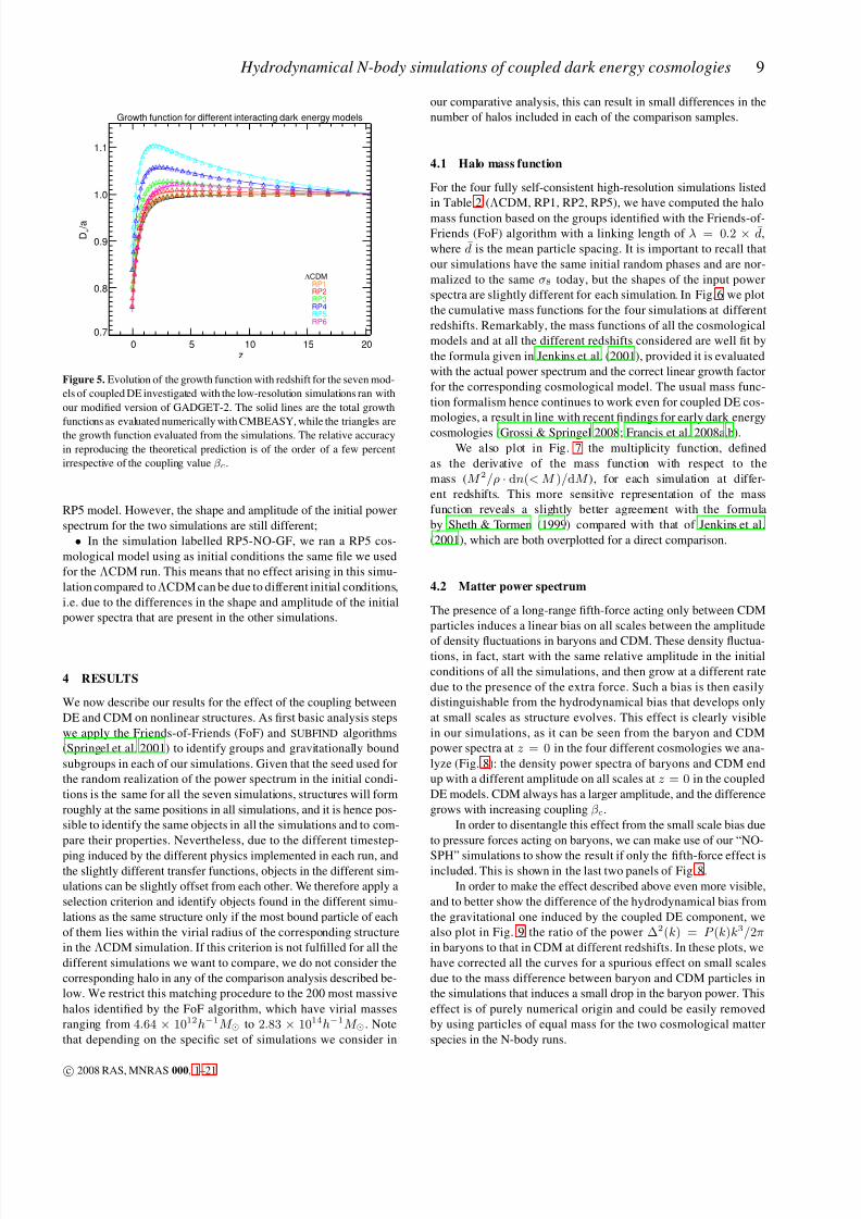
Figure 5. Evolution of the growth function with redshift for the seven mod-
els of coupled DE investigated with the low-resolution simulations ran with
our modified version of GADGET-2. The solid lines are the total growth
functions as evaluated numerically with CMBEASY, while the triangles arethe growth function evaluated from the simulations. The relative accuracy
in reproducing the theoretical prediction is of the order of a few percent
irrespective of the coupling value βc.
RP5 model. However, the shape and amplitude of the initial power
spectrum for the two simulations are still different;
• In the simulation labelled RP5-NO-GF, we ran a RP5 cos-
mological model using as initial conditions the same file we used
for the ΛCDM run. This means that no effect arising in this simu-
lation compared to ΛCDM can be due to different initial conditions,
i.e. due to the differences in the shape and amplitude of the initial
power spectra that are present in the other simulations.
4 RESULTS
We now describe our results for the effect of the coupling between
DE and CDM on nonlinear structures. As first basic analysis steps
we apply the Friends-of-Friends (FoF) and SUBFIND algorithms
(Springel et al. 2001) to identify groups and gravitationally bound
subgroups in each of our simulations. Given that the seed used for
the random realization of the power spectrum in the initial condi-
tions is the same for all the seven simulations, structures will form
roughly at the same positions in all simulations, and it is hence pos-
sible to identify the same objects in all the simulations and to com-
pare their properties. Nevertheless, due to the different timestep-
ping induced by the different physics implemented in each run, andthe slightly different transfer functions, objects in the different sim-
ulations can be slightly offset from each other. We therefore apply a
selection criterion and identify objects found in the different simu-
lations as the same structure only if the most bound particle of each
of them lies within the virial radius of the corresponding structure
in the ΛCDM simulation. If this criterion is not fulfilled for all the
different simulations we want to compare, we do not consider the
corresponding halo in any of the comparison analysis described be-
low. We restrict this matching procedure to the 200 most massive
halos identified by the FoF algorithm, which have virial masses
ranging from 4.64 × 10¹²h−1M ⊙ to 2.83 × 10¹⁴h−1M ⊙. Note
that depending on the specific set of simulations we consider in
our comparative analysis, this can result in small differences in the
number of halos included in each of the comparison samples.
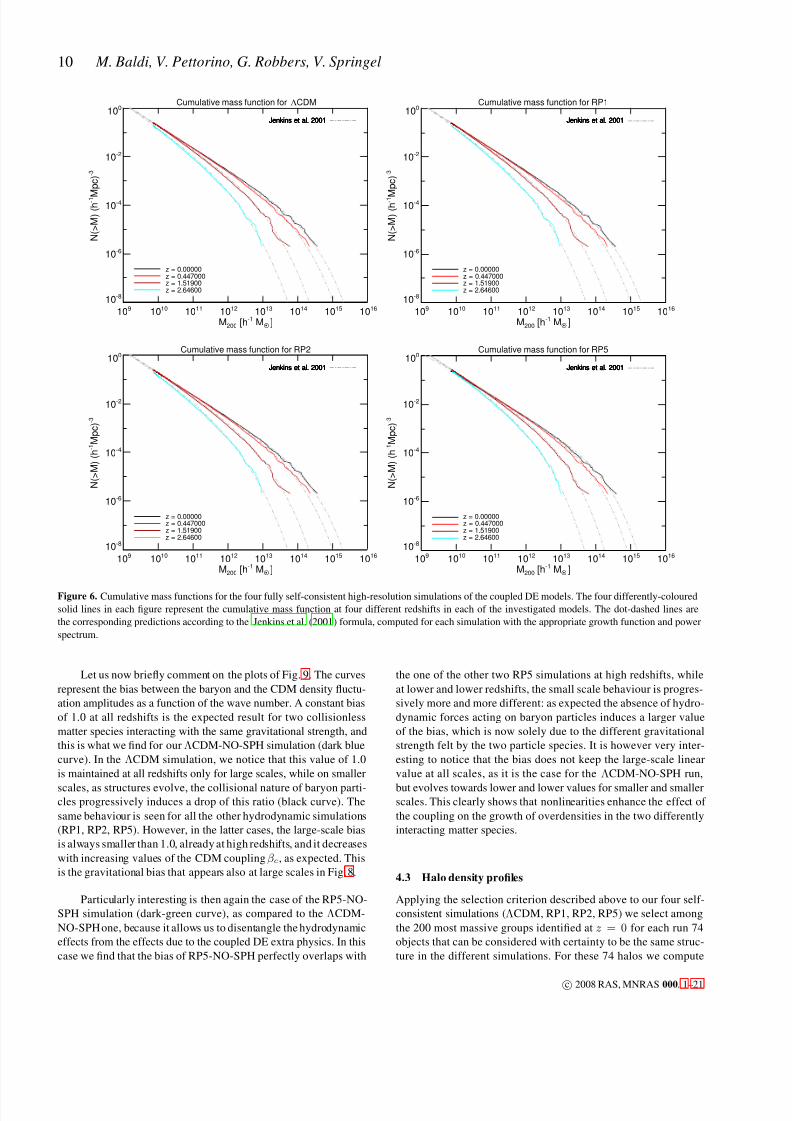
4.1 Halo mass function
For the four fully self-consistent high-resolution simulations listed
in Table 2 (ΛCDM, RP1, RP2, RP5), we have computed the halo
mass function based on the groups identified with the Friends-of-
Friends (FoF) algorithm with a linking length of λ = 0.2 × d,
where d is the mean particle spacing. It is important to recall that
our simulations have the same initial random phases and are nor-
malized to the same σ8 today, but the shapes of the input power
spectra are slightly different for each simulation. In Fig. 6 we plot
the cumulative mass functions for the four simulations at different
redshifts. Remarkably, the mass functions of all the cosmological
models and at all the different redshifts considered are well fit by
the formula given in Jenkins et al. (2001), provided it is evaluated
with the actual power spectrum and the correct linear growth factor
for the corresponding cosmological model. The usual mass func-
tion formalism hence continues to work even for coupled DE cos-
mologies, a result in line with recent findings for early dark energy
cosmologies (Grossi & Springel 2008; Francis et al. 2008a,b).
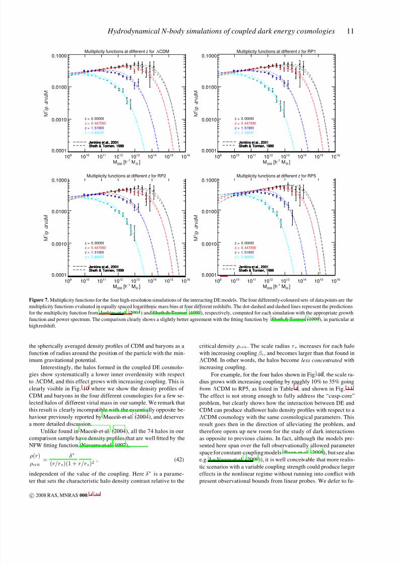
We also plot in Fig. 7 the multiplicity function, defined
as the derivative of the mass function with respect to the
mass (M 2/ρ · dn(< M )/dM ), for each simulation at differ-
ent redshifts. This more sensitive representation of the mass
function reveals a slightly better agreement with the formula
by Sheth & Tormen (1999) compared with that of Jenkins et al.
(2001), which are both overplotted for a direct comparison.
4.2 Matter power spectrum
The presence of a long-range fifth-force acting only between CDM
particles induces a linear bias on all scales between the amplitude
of density fluctuations in baryons and CDM. These density fluctua-tions, in fact, start with the same relative amplitude in the initial
conditions of all the simulations, and then grow at a different rate
due to the presence of the extra force. Such a bias is then easily
distinguishable from the hydrodynamical bias that develops only
at small scales as structure evolves. This effect is clearly visible
in our simulations, as it can be seen from the baryon and CDM
power spectra at z = 0 in the four different cosmologies we ana-
lyze (Fig. 8): the density power spectra of baryons and CDM end
up with a different amplitude on all scales at z = 0 in the coupled
DE models. CDM always has a larger amplitude, and the difference
grows with increasing coupling βc.
In order to disentangle this effect from the small scale bias due
to pressure forces acting on baryons, we can make use of our “NO-
SPH” simulations to show the result if only the fifth-force effect isincluded. This is shown in the last two panels of Fig. 8.
In order to make the effect described above even more visible,
and to better show the difference of the hydrodynamical bias from
the gravitational one induced by the coupled DE component, we
also plot in Fig. 9 the ratio of the power ∆2(k) = P (k)k3/2πin baryons to that in CDM at different redshifts. In these plots, we
have corrected all the curves for a spurious effect on small scales
due to the mass difference between baryon and CDM particles in
the simulations that induces a small drop in the baryon power. This
effect is of purely numerical origin and could be easily removed
by using particles of equal mass for the two cosmological matter
species in the N-body runs.
c 2008 RAS, MNRAS 000, 1–21
8/3/2019 Marco Baldi et al- Hydrodynamical N-body simulations of coupled dark energy cosmologies
http://slidepdf.com/reader/full/marco-baldi-et-al-hydrodynamical-n-body-simulations-of-coupled-dark-energy 10/21
10 M. Baldi, V. Pettorino, G. Robbers, V. Springel
Cumulative mass function for ΛCDM
109 1010 1011 1012 1013 1014 1015 1016
M200 [h-1 MO• ]
10-8
10-6
10-4
10-2
100
N ( > M ) ( h - 1 M
p c
) - 3
Jenkins et al. 2001Jenkins et al. 2001Jenkins et al. 2001Jenkins et al. 2001
z = 2.64600z = 1.51900z = 0.447000z = 0.00000
Cumulative mass function for RP1
109 1010 1011 1012 1013 1014 1015 1016
M200 [h-1 MO• ]
10-8
10-6
10-4
10-2
100
N ( > M ) ( h - 1 M
p c
) - 3
Jenkins et al. 2001Jenkins et al. 2001Jenkins et al. 2001Jenkins et al. 2001
z = 2.64600z = 1.51900z = 0.447000z = 0.00000
Cumulative mass function for RP2
109 1010 1011 1012 1013 1014 1015 1016
M200 [h-1 MO•
]
10-8
10-6
10-4
10-2
100
N ( > M ) ( h - 1 M p c
) - 3
Jenkins et al. 2001Jenkins et al. 2001Jenkins et al. 2001Jenkins et al. 2001
z = 2.64600z = 1.51900z = 0.447000z = 0.00000
Cumulative mass function for RP5
109 1010 1011 1012 1013 1014 1015 1016
M200 [h-1 MO•
]
10-8
10-6
10-4
10-2
100
N ( > M ) ( h - 1 M p c
) - 3
Jenkins et al. 2001Jenkins et al. 2001Jenkins et al. 2001Jenkins et al. 2001
z = 2.64600z = 1.51900z = 0.447000z = 0.00000
Figure 6. Cumulative mass functions for the four fully self-consistent high-resolution simulations of the coupled DE models. The four differently-coloured
solid lines in each figure represent the cumulative mass function at four different redshifts in each of the investigated models. The dot-dashed lines are
the corresponding predictions according to the Jenkins et al. (2001) formula, computed for each simulation with the appropriate growth function and power
spectrum.
Let us now briefly comment on the plots of Fig. 9. The curves
represent the bias between the baryon and the CDM density fluctu-
ation amplitudes as a function of the wave number. A constant bias
of 1.0 at all redshifts is the expected result for two collisionless
matter species interacting with the same gravitational strength, and
this is what we find for our ΛCDM-NO-SPH simulation (dark blue
curve). In the ΛCDM simulation, we notice that this value of 1.0
is maintained at all redshifts only for large scales, while on smaller
scales, as structures evolve, the collisional nature of baryon parti-cles progressively induces a drop of this ratio (black curve). The
same behaviour is seen for all the other hydrodynamic simulations
(RP1, RP2, RP5). However, in the latter cases, the large-scale bias
is always smaller than 1.0, already at high redshifts, and it decreases
with increasing values of the CDM coupling βc, as expected. This
is the gravitational bias that appears also at large scales in Fig. 8.
Particularly interesting is then again the case of the RP5-NO-
SPH simulation (dark-green curve), as compared to the ΛCDM-
NO-SPH one, because it allows us to disentangle the hydrodynamic
effects from the effects due to the coupled DE extra physics. In this
case we find that the bias of RP5-NO-SPH perfectly overlaps with
the one of the other two RP5 simulations at high redshifts, while
at lower and lower redshifts, the small scale behaviour is progres-
sively more and more different: as expected the absence of hydro-
dynamic forces acting on baryon particles induces a larger value
of the bias, which is now solely due to the different gravitational
strength felt by the two particle species. It is however very inter-
esting to notice that the bias does not keep the large-scale linear
value at all scales, as it is the case for the ΛCDM-NO-SPH run,
but evolves towards lower and lower values for smaller and smallerscales. This clearly shows that nonlinearities enhance the effect of
the coupling on the growth of overdensities in the two differently
interacting matter species.
4.3 Halo density profiles
Applying the selection criterion described above to our four self-
consistent simulations (ΛCDM, RP1, RP2, RP5) we select among
the 200 most massive groups identified at z = 0 for each run 74
objects that can be considered with certainty to be the same struc-
ture in the different simulations. For these 74 halos we compute
c 2008 RAS, MNRAS 000, 1–21
8/3/2019 Marco Baldi et al- Hydrodynamical N-body simulations of coupled dark energy cosmologies
http://slidepdf.com/reader/full/marco-baldi-et-al-hydrodynamical-n-body-simulations-of-coupled-dark-energy 11/21
Hydrodynamical N-body simulations of coupled dark energy cosmologies 11
Multiplicity functions at different z for ΛCDM
109 1010 1011 1012 1013 1014 1015 1016
M200 [h-1 MO• ]
0.0001
0.0010
0.0100
0.1000
M 2 / ρ
d n / d M
z = 0.00000
Sheth & Tormen, 1999Jenkins et al., 2001
z = 0.447000
Sheth & Tormen, 1999Jenkins et al., 2001
z = 1.51900
Sheth & Tormen, 1999Jenkins et al., 2001
z = 2.64600
Sheth & Tormen, 1999Jenkins et al., 2001
Multiplicity functions at different z for RP1
109 1010 1011 1012 1013 1014 1015 1016
M200 [h-1 MO• ]
0.0001
0.0010
0.0100
0.1000
M 2 / ρ
d n / d M
z = 0.00000
Sheth & Tormen, 1999Jenkins et al., 2001
z = 0.447000
Sheth & Tormen, 1999Jenkins et al., 2001
z = 1.51900
Sheth & Tormen, 1999Jenkins et al., 2001
z = 2.64600
Sheth & Tormen, 1999Jenkins et al., 2001
Multiplicity functions at different z for RP2
109 1010 1011 1012 1013 1014 1015 1016
M200 [h-1 MO•
]
0.0001
0.0010
0.0100
0.1000
M 2 / ρ
d n / d M
z = 0.00000
Sheth & Tormen, 1999Jenkins et al., 2001
z = 0.447000
Sheth & Tormen, 1999Jenkins et al., 2001
z = 1.51900
Sheth & Tormen, 1999Jenkins et al., 2001
z = 2.64600
Sheth & Tormen, 1999Jenkins et al., 2001
Multiplicity functions at different z for RP5
109 1010 1011 1012 1013 1014 1015 1016
M200 [h-1 MO•
]
0.0001
0.0010
0.0100
0.1000
M 2 / ρ
d n / d M
z = 0.00000
Sheth & Tormen, 1999Jenkins et al., 2001
z = 0.447000
Sheth & Tormen, 1999Jenkins et al., 2001
z = 1.51900
Sheth & Tormen, 1999Jenkins et al., 2001
z = 2.64600
Sheth & Tormen, 1999Jenkins et al., 2001
Figure 7. Multiplicity functions for the four high-resolution simulations of the interacting DE models. The four differently-coloured sets of data points are the
multiplicity functions evaluated in equally spaced logarithmic mass bins at four different redshifts. The dot-dashed and dashed lines represent the predictions
for the multiplicity function from Jenkins et al. (2001) and Sheth & Tormen (1999), respectively, computed for each simulation with the appropriate growth
function and power spectrum. The comparison clearly shows a slightly better agreement with the fitting function by Sheth & Tormen (1999), in particular at
high redshift.
the spherically averaged density profiles of CDM and baryons as a
function of radius around the position of the particle with the min-
imum gravitational potential.
Interestingly, the halos formed in the coupled DE cosmolo-
gies show systematically a lower inner overdensity with respect
to ΛCDM, and this effect grows with increasing coupling. This is
clearly visible in Fig. 10 where we show the density profiles of
CDM and baryons in the four different cosmologies for a few se-lected halos of different virial mass in our sample. We remark that
this result is clearly incompatible with the essentially opposite be-
haviour previously reported by Maccio et al. (2004), and deserves
a more detailed discussion.
Unlike found in Maccio et al. (2004), all the 74 halos in our
comparison sample have density profiles that are well fitted by the
NFW fitting function (Navarro et al. 1997)
ρ(r)
ρcrit=
δ∗
(r/rs)(1 + r/rs)2, (42)
independent of the value of the coupling. Here δ∗ is a parame-
ter that sets the characteristic halo density contrast relative to the
critical density ρcrit. The scale radius rs increases for each halo
with increasing coupling βc, and becomes larger than that found in
ΛCDM. In other words, the halos become less concentrated with
increasing coupling.
For example, for the four halos shown in Fig. 10, the scale ra-
dius grows with increasing coupling by roughly 10% to 35% going
from ΛCDM to RP5, as listed in Table 4, and shown in Fig. 11.
The effect is not strong enough to fully address the “cusp-core”problem, but clearly shows how the interaction between DE and
CDM can produce shallower halo density profiles with respect to a
ΛCDM cosmology with the same cosmological parameters. This
result goes then in the direction of alleviating the problem, and
therefore opens up new room for the study of dark interactions
as opposite to previous claims. In fact, although the models pre-
sented here span over the full observationally allowed parameter
space for constant-coupling models (Bean et al. (2008), but see also
e.g. La Vacca et al. (2009)), it is well conceivable that more realis-
tic scenarios with a variable coupling strength could produce larger
effects in the nonlinear regime without running into conflict with
present observational bounds from linear probes. We defer to fu-
c 2008 RAS, MNRAS 000, 1–21

8/3/2019 Marco Baldi et al- Hydrodynamical N-body simulations of coupled dark energy cosmologies
http://slidepdf.com/reader/full/marco-baldi-et-al-hydrodynamical-n-body-simulations-of-coupled-dark-energy 12/21
12 M. Baldi, V. Pettorino, G. Robbers, V. Springel
Power Spectrum of ΛCDM
0.1 1.0 10.0 100.0k [ h Mpc-1 ]
0.1
1.0
10.0
100.0
1000.0
10000.0
P ( k ) [ h - 3 M
p c
3 ]
z=0.00000
Dark MatterBaryons
z=0.00000
Dark MatterBaryons
z=0.00000
Dark MatterBaryons
Power Spectrum of RP1
0.1 1.0 10.0 100.0k [ h Mpc-1 ]
0.1
1.0
10.0
100.0
1000.0
10000.0
P ( k ) [ h - 3 M
p c
3 ]
z=0.00000
Dark MatterBaryons
z=0.00000
Dark MatterBaryons
z=0.00000
Dark MatterBaryons
Power Spectrum of RP2
0.1 1.0 10.0 100.0k [ h Mpc-1 ]
0.1
1.0
10.0
100.0
1000.0
10000.0
P ( k ) [ h - 3 M p c
3 ]
z=0.00000
Dark MatterBaryons
z=0.00000
Dark MatterBaryons
z=0.00000
Dark MatterBaryons
Power Spectrum of RP5
0.1 1.0 10.0 100.0k [ h Mpc-1 ]
0.1
1.0
10.0
100.0
1000.0
10000.0
P ( k ) [ h - 3 M p c
3 ]
z=0.00000
Dark MatterBaryons
z=0.00000
Dark MatterBaryons
z=0.00000
Dark MatterBaryons
Power Spectrum of ΛCDM NO SPH
0.1 1.0 10.0 100.0k [ h Mpc-1 ]
0.1
1.0
10.0
100.0
1000.0
10000.0
P ( k ) [ h - 3 M p c
3 ]
z=0.00000
Dark MatterBaryons
z=0.00000
Dark MatterBaryons
z=0.00000
Dark MatterBaryons
Power Spectrum of RP5 NO SPH
0.1 1.0 10.0 100.0k [ h Mpc-1 ]
0.1
1.0
10.0
100.0
1000.0
10000.0
P ( k ) [ h - 3 M p c
3 ]
z=0.00000
Dark MatterBaryons
z=0.00000
Dark MatterBaryons
z=0.00000
Dark MatterBaryons
Figure 8. Power spectra of CDM (black line) and baryons (blue line) at z = 0 for the set of coupled DE models under investigation. The appearance of a
bias between the two distributions, which grows with increasing coupling βc, is clearly visible at the large scale end of the plots. The last two panels show the
comparison of a ΛCDM and a coupled DE cosmology with βc = 0.2 in absence of hydrodynamic forces acting on baryons. In these two panels, the bias on
all scales is purely due to the interaction of CDM with the DE scalar field φ.
c 2008 RAS, MNRAS 000, 1–21

8/3/2019 Marco Baldi et al- Hydrodynamical N-body simulations of coupled dark energy cosmologies
http://slidepdf.com/reader/full/marco-baldi-et-al-hydrodynamical-n-body-simulations-of-coupled-dark-energy 13/21
Hydrodynamical N-body simulations of coupled dark energy cosmologies 13
0.1 1.0 10.0 100.0k [ h Mpc-1 ]
0.5
0.6
0.7
0.8
0.9
1.0
∆ 2 b ( k ) / ∆ 2 C D
M ( k )
RP5 NO SPHRP5 NO GFRP5RP2RP1ΛCDMΛCDM NO SPH
z=15.0000RP5 NO SPHRP5 NO GFRP5RP2RP1ΛCDMΛCDM NO SPH
z=15.0000RP5 NO SPHRP5 NO GFRP5RP2RP1ΛCDMΛCDM NO SPH
z=15.0000RP5 NO SPHRP5 NO GFRP5RP2RP1ΛCDMΛCDM NO SPH
z=15.0000RP5 NO SPHRP5 NO GFRP5RP2RP1ΛCDMΛCDM NO SPH
z=15.0000RP5 NO SPHRP5 NO GFRP5RP2RP1ΛCDMΛCDM NO SPH
z=15.0000RP5 NO SPHRP5 NO GFRP5RP2RP1ΛCDMΛCDM NO SPH
z=15.0000RP5 NO SPHRP5 NO GFRP5RP2RP1ΛCDMΛCDM NO SPH
z=15.0000RP5 NO SPHRP5 NO GFRP5RP2RP1ΛCDMΛCDM NO SPH
z=15.0000RP5 NO SPHRP5 NO GFRP5RP2RP1ΛCDMΛCDM NO SPH
z=15.0000RP5 NO SPHRP5 NO GFRP5RP2RP1ΛCDMΛCDM NO SPH
z=15.0000RP5 NO SPHRP5 NO GFRP5RP2RP1ΛCDMΛCDM NO SPH
z=15.0000RP5 NO SPHRP5 NO GFRP5RP2RP1ΛCDMΛCDM NO SPH
z=15.0000RP5 NO SPHRP5 NO GFRP5RP2RP1ΛCDMΛCDM NO SPH
z=15.0000RP5 NO SPHRP5 NO GFRP5RP2RP1ΛCDMΛCDM NO SPH
z=15.0000RP5 NO SPHRP5 NO GFRP5RP2RP1ΛCDMΛCDM NO SPH
z=15.0000RP5 NO SPHRP5 NO GFRP5RP2RP1ΛCDMΛCDM NO SPH
z=15.0000RP5 NO SPHRP5 NO GFRP5RP2RP1ΛCDMΛCDM NO SPH
z=15.0000RP5 NO SPHRP5 NO GFRP5RP2RP1ΛCDMΛCDM NO SPH
z=15.0000RP5 NO SPHRP5 NO GFRP5RP2RP1ΛCDMΛCDM NO SPH
z=15.0000RP5 NO SPHRP5 NO GFRP5RP2RP1ΛCDMΛCDM NO SPH
z=15.0000
0.1 1.0 10.0 100.0k [ h Mpc-1 ]
0.5
0.6
0.7
0.8
0.9
1.0
∆ 2 b ( k ) / ∆ 2 C D
M ( k )
RP5 NO SPHRP5 NO GFRP5RP2RP1ΛCDMΛCDM NO SPH
z=10.0552RP5 NO SPHRP5 NO GFRP5RP2RP1ΛCDMΛCDM NO SPH
z=10.0552RP5 NO SPHRP5 NO GFRP5RP2RP1ΛCDMΛCDM NO SPH
z=10.0552RP5 NO SPHRP5 NO GFRP5RP2RP1ΛCDMΛCDM NO SPH
z=10.0552RP5 NO SPHRP5 NO GFRP5RP2RP1ΛCDMΛCDM NO SPH
z=10.0552RP5 NO SPHRP5 NO GFRP5RP2RP1ΛCDMΛCDM NO SPH
z=10.0552RP5 NO SPHRP5 NO GFRP5RP2RP1ΛCDMΛCDM NO SPH
z=10.0552RP5 NO SPHRP5 NO GFRP5RP2RP1ΛCDMΛCDM NO SPH
z=10.0552RP5 NO SPHRP5 NO GFRP5RP2RP1ΛCDMΛCDM NO SPH
z=10.0552RP5 NO SPHRP5 NO GFRP5RP2RP1ΛCDMΛCDM NO SPH
z=10.0552RP5 NO SPHRP5 NO GFRP5RP2RP1ΛCDMΛCDM NO SPH
z=10.0552RP5 NO SPHRP5 NO GFRP5RP2RP1ΛCDMΛCDM NO SPH
z=10.0552RP5 NO SPHRP5 NO GFRP5RP2RP1ΛCDMΛCDM NO SPH
z=10.0552RP5 NO SPHRP5 NO GFRP5RP2RP1ΛCDMΛCDM NO SPH
z=10.0552RP5 NO SPHRP5 NO GFRP5RP2RP1ΛCDMΛCDM NO SPH
z=10.0552RP5 NO SPHRP5 NO GFRP5RP2RP1ΛCDMΛCDM NO SPH
z=10.0552RP5 NO SPHRP5 NO GFRP5RP2RP1ΛCDMΛCDM NO SPH
z=10.0552RP5 NO SPHRP5 NO GFRP5RP2RP1ΛCDMΛCDM NO SPH
z=10.0552RP5 NO SPHRP5 NO GFRP5RP2RP1ΛCDMΛCDM NO SPH
z=10.0552RP5 NO SPHRP5 NO GFRP5RP2RP1ΛCDMΛCDM NO SPH
z=10.0552RP5 NO SPHRP5 NO GFRP5RP2RP1ΛCDMΛCDM NO SPH
z=10.0552
0.1 1.0 10.0 100.0k [ h Mpc-1 ]
0.5
0.6
0.7
0.8
0.9
1.0
∆ 2 b ( k ) / ∆ 2 C
D M
( k )
RP5 NO SPHRP5 NO GFRP5RP2RP1ΛCDMΛCDM NO SPH
z=5.34949RP5 NO SPHRP5 NO GFRP5RP2RP1ΛCDMΛCDM NO SPH
z=5.34949RP5 NO SPHRP5 NO GFRP5RP2RP1ΛCDMΛCDM NO SPH
z=5.34949RP5 NO SPHRP5 NO GFRP5RP2RP1ΛCDMΛCDM NO SPH
z=5.34949RP5 NO SPHRP5 NO GFRP5RP2RP1ΛCDMΛCDM NO SPH
z=5.34949RP5 NO SPHRP5 NO GFRP5RP2RP1ΛCDMΛCDM NO SPH
z=5.34949RP5 NO SPHRP5 NO GFRP5RP2RP1ΛCDMΛCDM NO SPH
z=5.34949RP5 NO SPHRP5 NO GFRP5RP2RP1ΛCDMΛCDM NO SPH
z=5.34949RP5 NO SPHRP5 NO GFRP5RP2RP1ΛCDMΛCDM NO SPH
z=5.34949RP5 NO SPHRP5 NO GFRP5RP2RP1ΛCDMΛCDM NO SPH
z=5.34949RP5 NO SPHRP5 NO GFRP5RP2RP1ΛCDMΛCDM NO SPH
z=5.34949RP5 NO SPHRP5 NO GFRP5RP2RP1ΛCDMΛCDM NO SPH
z=5.34949RP5 NO SPHRP5 NO GFRP5RP2RP1ΛCDMΛCDM NO SPH
z=5.34949RP5 NO SPHRP5 NO GFRP5RP2RP1ΛCDMΛCDM NO SPH
z=5.34949RP5 NO SPHRP5 NO GFRP5RP2RP1ΛCDMΛCDM NO SPH
z=5.34949RP5 NO SPHRP5 NO GFRP5RP2RP1ΛCDMΛCDM NO SPH
z=5.34949RP5 NO SPHRP5 NO GFRP5RP2RP1ΛCDMΛCDM NO SPH
z=5.34949RP5 NO SPHRP5 NO GFRP5RP2RP1ΛCDMΛCDM NO SPH
z=5.34949RP5 NO SPHRP5 NO GFRP5RP2RP1ΛCDMΛCDM NO SPH
z=5.34949RP5 NO SPHRP5 NO GFRP5RP2RP1ΛCDMΛCDM NO SPH
z=5.34949RP5 NO SPHRP5 NO GFRP5RP2RP1ΛCDMΛCDM NO SPH
z=5.34949
0.1 1.0 10.0 100.0k [ h Mpc-1 ]
0.5
0.6
0.7
0.8
0.9
1.0
∆ 2 b ( k ) / ∆ 2 C
D M
( k )
RP5 NO SPHRP5 NO GFRP5RP2RP1ΛCDMΛCDM NO SPH
z=1.51974RP5 NO SPHRP5 NO GFRP5RP2RP1ΛCDMΛCDM NO SPH
z=1.51974RP5 NO SPHRP5 NO GFRP5RP2RP1ΛCDMΛCDM NO SPH
z=1.51974RP5 NO SPHRP5 NO GFRP5RP2RP1ΛCDMΛCDM NO SPH
z=1.51974RP5 NO SPHRP5 NO GFRP5RP2RP1ΛCDMΛCDM NO SPH
z=1.51974RP5 NO SPHRP5 NO GFRP5RP2RP1ΛCDMΛCDM NO SPH
z=1.51974RP5 NO SPHRP5 NO GFRP5RP2RP1ΛCDMΛCDM NO SPH
z=1.51974RP5 NO SPHRP5 NO GFRP5RP2RP1ΛCDMΛCDM NO SPH
z=1.51974RP5 NO SPHRP5 NO GFRP5RP2RP1ΛCDMΛCDM NO SPH
z=1.51974RP5 NO SPHRP5 NO GFRP5RP2RP1ΛCDMΛCDM NO SPH
z=1.51974RP5 NO SPHRP5 NO GFRP5RP2RP1ΛCDMΛCDM NO SPH
z=1.51974RP5 NO SPHRP5 NO GFRP5RP2RP1ΛCDMΛCDM NO SPH
z=1.51974RP5 NO SPHRP5 NO GFRP5RP2RP1ΛCDMΛCDM NO SPH
z=1.51974RP5 NO SPHRP5 NO GFRP5RP2RP1ΛCDMΛCDM NO SPH
z=1.51974RP5 NO SPHRP5 NO GFRP5RP2RP1ΛCDMΛCDM NO SPH
z=1.51974RP5 NO SPHRP5 NO GFRP5RP2RP1ΛCDMΛCDM NO SPH
z=1.51974RP5 NO SPHRP5 NO GFRP5RP2RP1ΛCDMΛCDM NO SPH
z=1.51974RP5 NO SPHRP5 NO GFRP5RP2RP1ΛCDMΛCDM NO SPH
z=1.51974RP5 NO SPHRP5 NO GFRP5RP2RP1ΛCDMΛCDM NO SPH
z=1.51974RP5 NO SPHRP5 NO GFRP5RP2RP1ΛCDMΛCDM NO SPH
z=1.51974RP5 NO SPHRP5 NO GFRP5RP2RP1ΛCDMΛCDM NO SPH
z=1.51974
0.1 1.0 10.0 100.0k [ h Mpc-1 ]
0.5
0.6
0.7
0.8
0.9
1.0
∆ 2 b ( k ) / ∆ 2 C
D M
( k )
RP5 NO SPH
RP5 NO GFRP5RP2RP1ΛCDMΛCDM NO SPH
z=0.00000RP5 NO SPH
RP5 NO GFRP5RP2RP1ΛCDMΛCDM NO SPH
z=0.00000RP5 NO SPH
RP5 NO GFRP5RP2RP1ΛCDMΛCDM NO SPH
z=0.00000RP5 NO SPH
RP5 NO GFRP5RP2RP1ΛCDMΛCDM NO SPH
z=0.00000RP5 NO SPH
RP5 NO GFRP5RP2RP1ΛCDMΛCDM NO SPH
z=0.00000RP5 NO SPH
RP5 NO GFRP5RP2RP1ΛCDMΛCDM NO SPH
z=0.00000RP5 NO SPH
RP5 NO GFRP5RP2RP1ΛCDMΛCDM NO SPH
z=0.00000RP5 NO SPH
RP5 NO GFRP5RP2RP1ΛCDMΛCDM NO SPH
z=0.00000RP5 NO SPH
RP5 NO GFRP5RP2RP1ΛCDMΛCDM NO SPH
z=0.00000RP5 NO SPH
RP5 NO GFRP5RP2RP1ΛCDMΛCDM NO SPH
z=0.00000RP5 NO SPH
RP5 NO GFRP5RP2RP1ΛCDMΛCDM NO SPH
z=0.00000RP5 NO SPH
RP5 NO GFRP5RP2RP1ΛCDMΛCDM NO SPH
z=0.00000RP5 NO SPH
RP5 NO GFRP5RP2RP1ΛCDMΛCDM NO SPH
z=0.00000RP5 NO SPH
RP5 NO GFRP5RP2RP1ΛCDMΛCDM NO SPH
z=0.00000RP5 NO SPH
RP5 NO GFRP5RP2RP1ΛCDMΛCDM NO SPH
z=0.00000RP5 NO SPH
RP5 NO GFRP5RP2RP1ΛCDMΛCDM NO SPH
z=0.00000RP5 NO SPH
RP5 NO GFRP5RP2RP1ΛCDMΛCDM NO SPH
z=0.00000RP5 NO SPH
RP5 NO GFRP5RP2RP1ΛCDMΛCDM NO SPH
z=0.00000RP5 NO SPH
RP5 NO GFRP5RP2RP1ΛCDMΛCDM NO SPH
z=0.00000RP5 NO SPH
RP5 NO GFRP5RP2RP1ΛCDMΛCDM NO SPH
z=0.00000RP5 NO SPH
RP5 NO GFRP5RP2RP1ΛCDMΛCDM NO SPH
z=0.00000
Figure 9. Ratio of the power spectra of baryons and CDM as a function of wavenumber for the set of high-resolution simulations ran with our modified version
of GADGET-2, for five different redshifts. The linear large-scale bias appears already at high redshifts, while at lower redshifts the hydrodynamic forces start
to suppress power in the baryon component at small scales. In absence of such hydrodynamic forces the progressive enhancement of the large scale bias at
small scales for the RP5-NO-SPH run (light green curve) as compared to the completely flat behaviour of the ΛCDM-NO-SPH simulation (blue curve) –
where no bias is expected – shows clearly that nonlinearities must increase the effect of the coupling on the different clustering rates of the two species. All
the curves have been corrected for a spurious numerical drop of the baryonic power at small scales as described in the text.
c 2008 RAS, MNRAS 000, 1–21

8/3/2019 Marco Baldi et al- Hydrodynamical N-body simulations of coupled dark energy cosmologies
http://slidepdf.com/reader/full/marco-baldi-et-al-hydrodynamical-n-body-simulations-of-coupled-dark-energy 14/21
14 M. Baldi, V. Pettorino, G. Robbers, V. Springel
Halo Density profiles for CDM and baryons for Group nr. 0
10 100 1000R (h-1 kpc)
101
102
103
104
105
ρ / ρ
c r i t
M200(ΛCDM) = 2.82510e+14 h-1 MO•
ΛCDMRP1RP2RP5
ΛCDMRP1RP2RP5
ΛCDMRP1RP2RP5
ΛCDMRP1RP2RP5
Halo Density profiles for CDM and baryons for Group nr. 29
10 100 1000R (h-1 kpc)
10
100
1000
10000
ρ / ρ
c r i t
M200(ΛCDM) = 2.79752e+13 h-1 MO•
ΛCDMRP1RP2RP5
ΛCDMRP1RP2RP5
ΛCDMRP1RP2RP5
ΛCDMRP1RP2RP5
Halo Density profiles for CDM and baryons for Group nr. 60
10 100 1000R (h-1 kpc)
10
100
1000
10000
ρ / ρ
c r i t
M200(ΛCDM) = 1.70238e+13 h-1 MO•
ΛCDMRP1
RP2RP5
ΛCDMRP1
RP2RP5
ΛCDMRP1
RP2RP5
ΛCDMRP1
RP2RP5
Halo Density profiles for CDM and baryons for Group nr. 175
10 100R (h-1 kpc)
10
100
1000
10000
ρ / ρ
c r i t
M200(ΛCDM) = 6.51036e+12 h-1 MO•
ΛCDMRP1
RP2RP5
ΛCDMRP1
RP2RP5
ΛCDMRP1
RP2RP5
ΛCDMRP1
RP2RP5
Figure 10. Density profiles of CDM (solid lines) and baryons (dot-dashed lines) for four halos of different mass in the simulation box at z = 0. The vertical
dot-dashed line indicates the location of the virial radius for the ΛCDM halo. The decrease of the inner overdensity of the profiles with increasing coupling is
clearly visible in all the four plots.
ture work the investigation of such models, but we stress here that
our present results constitute the first evidence that the nonlinear
dynamics of generalized coupled cosmologies might provide a so-
lution to the “cusp-core” problem.
4.4 Halo concentrations
For all the 200 most massive halos found in each of our four fully
self consistent simulations we compute halo concentrations as
c =r200
rs, (43)
based on our NFW fits to the halo density profiles. Here r200 is the
radius enclosing a mean overdensity 200 times the critical density.
Note that here no further selection criterion is applied, and the con-
centration is computed for all the 200 most massive halos in each
simulation.
Consistently with the trend found for the inner overdensity in
the halo density profiles and for the evolution of the scale radius
Evolution of halo scale radius with coupling
0.00 0.05 0.10 0.15 0.20βc
0.6
0.8
1.0
1.2
1.4
r s ( β c ) / r s
, Λ C D M
Group nr. 175Group nr. 60Group nr. 29Group nr. 0
Figure 11. Relative evolution with respect to ΛCDM of the scale radius rsfor the four halos plotted in Fig. 10 as a function of coupling βc.
c 2008 RAS, MNRAS 000, 1–21

8/3/2019 Marco Baldi et al- Hydrodynamical N-body simulations of coupled dark energy cosmologies
http://slidepdf.com/reader/full/marco-baldi-et-al-hydrodynamical-n-body-simulations-of-coupled-dark-energy 15/21
Hydrodynamical N-body simulations of coupled dark energy cosmologies 15
Group 0
rs (h−1 kpc)
Group 0rs
rs(ΛCDM)
Group 29
rs (h−1 kpc)
Group 29rs
rs(ΛCDM)
Group 60
rs (h−1 kpc)
Group 60rs
rs(ΛCDM)
Group 175
rs (h−1 kpc)
Group 175rs
rs(ΛCDM)
ΛCDM 225.14 1.0 105.51 1.0 61.92 1.0 70.61 1.0
RP1 229.00 1.02 120.21 1.14 61.16 0.99 67.45 0.96
RP2 233.96 1.04 119.68 1.13 63.52 1.03 70.48 1.0
RP5 295.47 1.31 143.92 1.36 73.46 1.19 76.26 1.08
Table 4. Evolution of the scale radius rs for the four halos shown in Fig. 10 with respect to the corresponding ΛCDM value. The trend is towards larger values
of rs
with increasing coupling βc
, with a relative growth of up to 36% for the largest coupling value βc
= 0.2.
with coupling, we find that halo concentrations are on average sig-
nificantly lower for coupled DE models with respect to ΛCDM,
and the effect again increases with increasing coupling βc. This
behaviour is shown explicitly in the left panel of Fig. 12, where
we plot halo concentrations as a function of the halo virial mass
M 200 for a series of our high-resolution simulations. In the stan-
dard interpretation, the halo concentrations are thought to reflect
the cosmic matter density at the time of formation of the halo, lead-
ing to the association of a larger value of the concentration with
an earlier formation epoch, and vice versa. In the context of this
standard picture, the effect we found for the concentrations could
be interpreted as a sign of a later formation time of massive ha-
los in the coupled DE models as compared to the ΛCDM model.
Such a later formation time could be possibly due to the fact that
matter density fluctuations start with a lower amplitude in the ini-
tial conditions of the coupled cosmologies with respect to ΛCDM,
and this would make them forming massive structures later, despite
their faster linear growth (as shown in Fig. 5).
However, we can demonstrate that this is not the case, just
making use of our RP5-NO-GF simulation, in which the Universe
evolves according to the same physics as RP5, but starting with the
identical initial conditions as used for the ΛCDM run. Therefore,
any difference between these two simulations can not be due to the
initial amplitude of fluctuations. The evolution of halo concentra-
tions with mass for this run is also plotted in Fig. 12 (dark blue
curve), and shows a very similar behaviour to the RP5 curve.
As a cross check of this result, we have repeated the same anal-
ysis by computing halo concentrations with an independent method
that circumvents the profile fitting. The concentration can be re-
lated to two other basic structural properties of a halo, namely its
maximum rotational velocity V max, and the radius at which this
velocity peak is located, rmax. According to Springel et al. (2008),
the concentration can then be related to these two quantities by the
relation:
200
3
c3
ln(1 + c)− c/(1 + c)= 7.213 δV , (44)
where δV is a simple function of V max and rmax:
δV = 2 V max
H 0rmax
2
. (45)
We denote the concentrations evaluated in this way as c∗, and in-
clude our results as a function of halo mass in the right panel of
Fig. 12. Although not identical in detail, as expected due to the
different methods used to measure concentrations, the two plots
of Fig. 12 show the same trend for the evolution of halo concen-
trations with coupling, and the same independence of this effect
from the initial conditions of the simulations. The slight down-turn
of the concentrations curve at the low-mass end that is visible in
both the two panels of Fig. 12 is an expected effect due to nu-
merical resolution, as was discussed in detail in Neto et al. (2007)
and in Springel et al. (2008). Although the concentration decrease
is found to have the same trend and amplitude for the poorly re-
Mean formation redshift fordifferent coupled dark energy models
1013 1014
M200 [h-1 MO•
]
0.2
0.4
0.6
0.8
1.0
1.2
z f
ΛCDMRP1RP2RP5
Figure 13. Evolution of the mean halo formation redshift zf as a function
of halo mass for the 200 most massive halos in our simulations and for the
different cosmological models under investigation. The formation redshift
zf is defined as the redshift at which the main progenitor of the halo has a
virial mass equal to half the virial mass of the halo at z = 0 . The halos have
been binned by mass, and the mean formation redshift in each bin is plotted
as a filled circle. The coloured dashed lines indicate for each simulation the
spread of 68% of the halos in each mass bin. The highest mass bin is not
plotted because of its too low number of halos.
solved low-mass halos as for the larger structures for which no res-
olution problem is expected, one should keep in mind as an element
of caution that higher resolution simulations would be required for
a definitive confirmation of this effect in the low-mass range of our
comparison sample, i.e. for masses below 1013 M⊙ /h.
In order to directly verify that the lower concentrations cannot
be a consequence of a later formation time we have also computed
the average formation redshift of the halos in our sample for all the
four self-consistent simulations, by building merger trees for all the
halos in our sample, and by following backwards in time the main
progenitor of each halo until the redshift at which its virial mass isonly half of the final virial mass of the halo at z = 0. We define the
corresponding time as the formation redshift zf of the halo.
In Figure 13, we show the evolution of zf as a function of
halo mass for all our cosmological models. It is evident that mas-
sive halos in the different cosmologies form approximately at the
same time, with a slightly earlier formation for the RP5 cosmol-
ogy, which one might have expected to translate into slightly larger
values of the concentrations. Therefore we conclude that the un-
ambiguous trend of lower halo concentrations for larger coupling
values must be a peculiar feature that arises from the extra physics
that characterizes the coupled DE cosmologies. A more detailed in-
vestigation of how this peculiar behaviour arises is hence required
c 2008 RAS, MNRAS 000, 1–21

8/3/2019 Marco Baldi et al- Hydrodynamical N-body simulations of coupled dark energy cosmologies
http://slidepdf.com/reader/full/marco-baldi-et-al-hydrodynamical-n-body-simulations-of-coupled-dark-energy 16/21
16 M. Baldi, V. Pettorino, G. Robbers, V. Springel
1013 1014
M200 [h-1 MO• ]
2
3
4
5
6
7
c m e a n
ΛCDMRP1RP2RP5
RP5 NO GF
1013 1014
M200 [h-1 MO• ]
2
3
4
5
6
7
c * m
e a n
ΛCDMRP1RP2RP5
RP5 NO GF
Figure 12. Evolution of the mean halo concentration as a function of mass for the 200 most massive halos in our simulations and for the different cosmological
models under investigation. The concentrations have been computed by directly fitting the halo density profile of each halo with an NFW model (left panel)
or by using the method introduced by Springel et al. (2008) and described in Eqs. (44,45) (right panel). The halos have been binned by mass, and the mean
concentration in each bin is plotted as a filled circle. The coloured dashed lines indicate for each simulation the spread of 68% of the halos in each mass bin.The highest mass bin is not plotted because of its very low number of halos. The decrease of the mean concentration with increasing coupling appears in the
same way in both plots.
in order to understand this phenomenology of the dynamics in cou-
pled DE cosmologies.
We perform such an investigation by switching off individu-
ally the two main effects which could be responsible of the con-
centrations drop, which are the variation of particle mass and the
extra velocity-dependent term. To save computational time, we do
this only for the most strongly coupled model RP5 and only for
the late stages of cosmic evolution. More specifically, we take one
of our RP5 simulation snapshots at a given redshift z∗, and use it
as initial conditions file for a new run starting at z = z∗ down to
z = 0 in which one of these two effects is switched off. We la-
bel these simulations as “RP5-NO-MASS” and “RP5-NO-FRIC”
for the cases where the mass decrease or the velocity-dependent
term are dropped, respectively. We set z∗ = 1.5 as a conservative
choice based on the consideration that, according to our definition
of formation redshift of a halo, all the halos in our sample have a
formation redshift z < z∗, as shown in Fig. 13.
By switching off the mass variation for z < z∗, we find that
the halo concentrations at z = 0 show a slight increase over the
whole mass range of the sample with respect to the fully self-
consistent RP5 simulation. This effect is shown in the left panel of
Fig. 14. We interpret this as a sign of the fact that the mass decrease
reduces the total gravitational potential energy of halos, resulting in
a modification of their virial equilibrium configuration.In fact, if the potential well of a halo gets shallower as time
goes by as a consequence of the decrease of the mass of its CDM
content, the system will find itself with an excess of kinetic en-
ergy, and will therefore expand in order to restore virial equilib-
rium. Such an expansion is expected to cause a drop of the halo
concentrations, which we confirm here because switching off this
mechanisms yields consistently higher concentrations at z = 0.
However, it is clear from Fig. 14 that this mechanism cannot ac-
count for the total effect of concentration decrease, but only for a
small fraction of it.
We therefore now investigate the other possible origin of this
effect, i.e. the impact of the velocity-dependent term (29) on the dy-
namics of CDM particles. To this end we switch off for z < z∗ the
additional acceleration arising from the velocity-dependent term
for coupled particles described by Eqn. (3.1.3). The outcome of this
test simulation is shown in the right panel of Fig. 14: the increase
of the concentrations with respect to the fully self-consistent RP5
simulation is now much more substantial than in the case of RP5-
NO-MASS, and shows that the velocity-dependent term is actually
the dominant mechanism in determining the decrease of halo con-
centrations and the decrease of the inner overdensity of CDM halos
discussed above. The interpretation of this effect seems quite un-
ambiguous: the velocity-dependent term induces an extra accelera-
tion on coupled particles in the direction of their velocity, and this
produces an increase of the kinetic energy of the particles, moving
the system out of its virial equilibrium configuration. The system
responds by a small expansion and a lowering of the concentration.
As a further check of this interpretation of our results, we also
test directly the dynamic evolution of halos to check whether they
really slightly expand in the presence of DE-CDM coupling. To this
end, we compute for all the halos in our sample the time evolution
of the mass and the number of particles contained in a sphere of
physical radius r = 20 h−1kpc centred on the potential minimum
of each halo. This sphere represents the very innermost part of all
the halos in our sample at any redshift between z∗ and 0, and we
refer to it as the halo “core”; its mass content is expected to beroughly constant for ΛCDM cosmologies at low redshifts. Indeed,
we can recover this behaviour for our ΛCDM simulation by aver-
aging the evolution of core masses and particle numbers over the
whole halo sample. On the other hand, for RP5, as expected ac-
cording to our interpretation, both the mass and the number of par-
ticles in the halo cores strongly decrease with time. This is shown
in Fig. 15, where the solid lines represent the average evolution of
mass, and the dashed lines represent the average evolution of the
particle number. Evidently, for ΛCDM the two curves coincide be-
cause the mass of the particles is constant and any change of the
enclosed mass in the core must be due to a change of the number
of enclosed particles. On the other hand, for RP5, the mass and
c 2008 RAS, MNRAS 000, 1–21
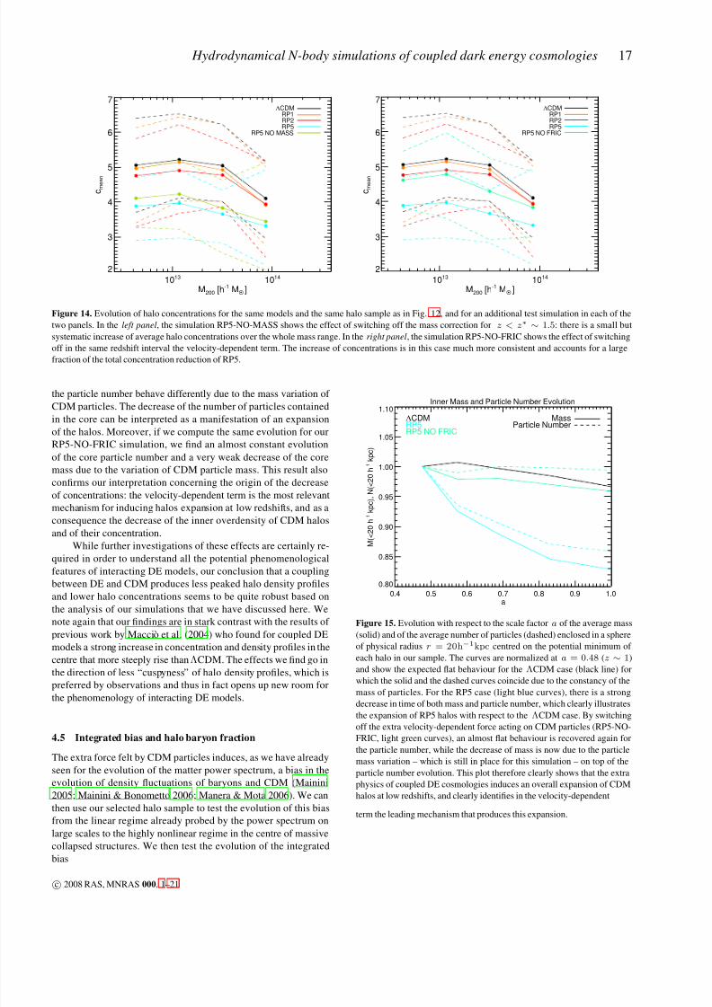
8/3/2019 Marco Baldi et al- Hydrodynamical N-body simulations of coupled dark energy cosmologies
http://slidepdf.com/reader/full/marco-baldi-et-al-hydrodynamical-n-body-simulations-of-coupled-dark-energy 17/21

8/3/2019 Marco Baldi et al- Hydrodynamical N-body simulations of coupled dark energy cosmologies
http://slidepdf.com/reader/full/marco-baldi-et-al-hydrodynamical-n-body-simulations-of-coupled-dark-energy 18/21
18 M. Baldi, V. Pettorino, G. Robbers, V. Springel
B(< r ) ≡ρb(< r )− ρb
ρb·
ρcρc(< r)− ρc
, (46)
as defined in Maccio et al. (2004), where ρb(< r) and ρc(< r)are the densities within a sphere of radius r around the potential
minimum of a halo, for baryons and CDM, respectively. Following
Maccio et al. (2004), we have not used the innermost part of the ha-
los (r < 10h−1kpc ∼ 3×ǫs) in order to avoid potential resolution
problems.In Figure 16, we show the evolution of the bias for four se-
lected halos of our sample with similar masses as the ones shown
in Fig. 10. It clearly appears that the bias is considerably enhanced
in the nonlinear regime, while at large scales it converges to the
linear value evaluated from the power spectrum amplitude on large
scales, represented in Fig. 16 by the horizontal dashed lines.
However, also in this case this effect could be due only to the
presence of hydrodynamical forces acting on the baryons, and may
not really be caused by the fifth-forces from the coupled DE scalar
field, as we can infer from the fact that also the ΛCDM curve,
where no coupled DE is present, shows a departure from the large
scale value of 1.0 when approaching the centre of the halos. Once
again we make use of our additional test simulations ΛCDM-NO-
SPH and RP5-NO-SPH in order to disentangle the two effects. InFig. 17, we show the same four plots as in Fig. 16 for the two simu-
lations without hydrodynamic forces, and the appearance of a non-
linear bias imprinted only by the coupled DE scalar field acting on
CDM particles is then absolutely evident. On the other hand, the ab-
sence of any bias, as expected, in the ΛCDM-NO-SPH run shows
clearly that no major numerical problems can be responsible for the
effect in the RP5-NO-SPH simulations. This evolution of the bias
B(< r) with radius for massive halos is in good agreement with
that found by Maccio et al. (2004) despite the starkly different be-
havior of the individual overdensities in baryons and CDM found
in the two works.
It is interesting that the above effect produces a baryon deficit
in virialized halos, i.e. they contain fewer baryons than expected
based on their mass and the universal cosmological baryon fraction.
In particular, this means that one can not expect that baryon frac-
tions determined through X-ray measurements in clusters would
yield the cosmological value. It is important to stress again here
that our approach does not include non-adiabatic processes (like
e.g. star formation, cooling, and possible feedback mechanisms)
to the physics of the baryonic component. Therefore our outcomes
cannot be expected to provide a prediction of baryon fractions to be
directly confronted with observations. However, this approach has
the advantage to clearly show in which direction the DE coupling
affects the baryon budget of collapsed structures which would then
be available for such radiative processes. In order to give a rough
estimate of the magnitude of this effect we compute the baryon
fraction within the virial radius r200 of all the halos in our sample
defined as
f b ≡M b(< r200)
M tot(< r200)(47)
for our four fully self-consistent simulations. We plot in Fig. 18 as
a function of halo virial mass the relative baryon fraction defined
as:
Y b ≡f b
Ωb/Ωm. (48)
For the ΛCDM case, our results for the evolution of Y b are consis-
tent with the value of Y b ∼ 0.92 found by the Santa Barbara Clus-
ter Comparison Project (Frenk et al. 1999), and with the more re-
Evolution of the relative baryon fraction with mass
1013 1014
M200 [h-1 MO• ]
0.80
0.85
0.90
0.95
1.00
Y b
RP5RP2RP1
ΛCDM
Figure 18. Evolution with virial mass M 200 of the relative baryon fraction
Y b within the virial radius r200 of all the halos in our sample. The coloured
diamonds represent the relative baryon fraction of each single halo, while
the filled circles and the coloured curves show the behaviour of the meanrelative baryon fraction in each mass bin for the four fully self-consistent
high-resolution simulations. A decrease of Y b with increasing coupling is
clearly visible both in the distribution of the individual halos and in the
averaged curves.
cent results of Ettori et al. (2006) and Gottloeber & Yepes (2007),
while for the coupled models the relative baryon fraction shows a
progressive decrease with increasing coupling, down to a value of
Y b ∼ 0.86 − 0.87 for the RP5 case.
It is also important to notice that this effect is always to-
wards lower baryon fractions in clusters with respect to the cos-
mological value. This could in fact alleviate tensions between the
high baryon abundance estimated from CMB observations, and
the somewhat lower values inferred from detailed X-ray obser-vations of galaxy clusters (Vikhlinin et al. 2006; McCarthy et al.
2007; LaRoque et al. 2006; Afshordi et al. 2007).
5 CONCLUSIONS
We have investigated coupled DE cosmologies, both with respect
to their expected background and linear perturbation evolution, as
well as in their predictions for the nonlinear regime of structure
formation. To do so we have developed and tested in this work a
modified version of the cosmological N-body code GADGET-2 sui-
table for evolving these kinds of cosmological models. The nume-
rical implementation we have developed is in fact quite general and
not restricted to the simple specific models of coupled quintessence
that we have investigated in this paper. Instead, it should be well
suited for a much wider range of DE models. We also note that
the ability to selectively enable or disable each of the modifications
discussed above, makes the code suitable for cosmological models
that are unrelated to the coupled DE scenario but require similar
new degrees of freedom that our implementation allows. These are:
(i) the expansion history of the Universe can be specified ac-
cording to any desired evolution of the Hubble rate as a function of
the scale factor a;
(ii) a global variation in time of the gravitational constant and/or
a variation in time of the gravitational strength for each individual
c 2008 RAS, MNRAS 000, 1–21

8/3/2019 Marco Baldi et al- Hydrodynamical N-body simulations of coupled dark energy cosmologies
http://slidepdf.com/reader/full/marco-baldi-et-al-hydrodynamical-n-body-simulations-of-coupled-dark-energy 19/21
Hydrodynamical N-body simulations of coupled dark energy cosmologies 19
Integrated Bias for Group nr. 1
1000 2000 3000 4000 5000 6000R (h-1 kpc)
0.5
0.6
0.7
0.8
0.9
1.0
B ( <
R )
z = 0.00000
M200(ΛCDM) = 1.57836e+14 h-1 MO•
ΛCDMRP1RP2RP5
z = 0.00000
ΛCDMRP1RP2RP5
z = 0.00000
ΛCDMRP1RP2RP5
z = 0.00000
ΛCDMRP1RP2RP5
Integrated Bias for Group nr. 33
1000 2000 3000 4000 5000 6000R (h-1 kpc)
0.5
0.6
0.7
0.8
0.9
1.0
B ( <
R )
z = 0.00000
M200(ΛCDM) = 2.76456e+13 h-1 MO•
ΛCDMRP1RP2RP5
z = 0.00000
ΛCDMRP1RP2RP5
z = 0.00000
ΛCDMRP1RP2RP5
z = 0.00000
ΛCDMRP1RP2RP5
Integrated Bias for Group nr. 76
1000 2000 3000 4000 5000 6000R (h-1 kpc)
0.5
0.6
0.7
0.8
0.9
1.0
B ( < R )
z = 0.00000
M200(ΛCDM) = 1.10487e+13 h-1 MO•
ΛCDMRP1RP2RP5
z = 0.00000
ΛCDMRP1RP2RP5
z = 0.00000
ΛCDMRP1RP2RP5
z = 0.00000
ΛCDMRP1RP2RP5
Integrated Bias for Group nr. 169
1000 2000 3000 4000 5000 6000R (h-1 kpc)
0.5
0.6
0.7
0.8
0.9
1.0
B ( < R )
z = 0.00000
M200(ΛCDM) = 7.78954e+12 h-1 MO•
ΛCDMRP1RP2RP5
z = 0.00000
ΛCDMRP1RP2RP5
z = 0.00000
ΛCDMRP1RP2RP5
z = 0.00000
ΛCDMRP1RP2RP5
Figure 16. Evolution of the integrated bias B(< r) for the four fully self-consistent high-resolution simulations and for four selected halos of different mass
in our sample. The horizontal dashed lines indicate the value of the large scale linear bias as evaluated from the power spectrum amplitudes of baryons and
CDM. The vertical black dot-dashed line shows the position of the virial radius for the ΛCDM halo in the sample. The drop of the value of B(< r) in the
innermost regions of the halos is evident but in these runs is given by a superposition of effects due to hydrodynamical forces and to the modified gravitational
interaction. On large scales, the bias tends to converge to the linear value, as expected.
matter species. This includes the possibility to have a long range
repulsive interaction between different particle species;
(iii) variation in time of the particle mass of each individual mat-
ter species;
(iv) extra velocity-dependent terms in the equation of motion for
each individual matter species.
With this implementation we have investigated the effects of
coupled DE models with a constant coupling βc to the CDM fluid
on structure formation. We have shown that the halo mass func-
tion is modified in coupled DE models, but can still be well fitted
at different redshifts by the Jenkins et al. (Jenkins et al. 2001) fit-ting formula, or by the Sheth & Tormen (Sheth & Tormen 1999)
formula, which yields a moderately better agreement, especially at
z > 0.
We have confirmed the analytic prediction that density fluc-
tuations in baryons and CDM will develop a bias on all scales due
to the presence of a fifth-force acting only between CDM particles.
We have also shown that in addition to this the bias is enhanced
when moving from the linear regime of very large scales to smaller
and progressively more non-linear scales.
We have investigated the evolution of the bias between
baryons and CDM overdensities down to the very nonlinear regime
found in the inner part of collapsed objects, in the same fashion
as described in Maccio et al. (2004). We found here similar results
with this previous work, namely an enhancement of the bias in the
nonlinear region within and around massive halos. We also recover
from this analysis the large scale value of the linear bias computed
from the power spectrum when integrating the bias function up to
very large radii from the centre of CDM halos. The enhancement of
the bias in highly nonlinear structures has an impact on the deter-
mination of the baryon fraction from cluster measurements, and we
have computed for all our halos, without including non-adiabatic
processes, the evolution of this fraction within the virial radius r200
with coupling, finding that the baryon fraction is reduced with in-
creasing coupling by up to ∼ 8− 10% with respect to ΛCDM forthe largest coupling value.
We have also investigated the effectof the coupling on the halo
density profiles. We find that they are remarkably well fit over the
resolved range by the NFW formula for any value of the coupling.
There is a clear trend of a decrease of the inner halo overdensity
with respect to ΛCDM with increasing coupling (or, equivalently,
an increase of the scale radius rs for increasing coupling). This
result conflicts with previous claims for the same class of coupled
DE models (Maccio et al. 2004).
Using a number of special test simulations, we have identified
the origin of this effect of reduced halo concentrations for increas-
c 2008 RAS, MNRAS 000, 1–21

8/3/2019 Marco Baldi et al- Hydrodynamical N-body simulations of coupled dark energy cosmologies
http://slidepdf.com/reader/full/marco-baldi-et-al-hydrodynamical-n-body-simulations-of-coupled-dark-energy 20/21
20 M. Baldi, V. Pettorino, G. Robbers, V. Springel
Integrated Bias for Group nr. 1
1000 2000 3000 4000 5000 6000R (h-1 kpc)
0.5
0.6
0.7
0.8
0.9
1.0
B ( <
R )
z = 0.00000
M200(ΛCDM) = 1.57836e+14 h-1 MO•
ΛCDMΛCDM NO SPH
RP5 NO SPH
z = 0.00000
ΛCDMΛCDM NO SPH
RP5 NO SPH
z = 0.00000
ΛCDMΛCDM NO SPH
RP5 NO SPH
Integrated Bias for Group nr. 33
1000 2000 3000 4000 5000 6000R (h-1 kpc)
0.5
0.6
0.7
0.8
0.9
1.0
B ( <
R )
z = 0.00000
M200(ΛCDM) = 2.76456e+13 h-1 MO•
ΛCDMΛCDM NO SPH
RP5 NO SPH
z = 0.00000
ΛCDMΛCDM NO SPH
RP5 NO SPH
z = 0.00000
ΛCDMΛCDM NO SPH
RP5 NO SPH
Integrated Bias for Group nr. 76
1000 2000 3000 4000 5000 6000R (h-1 kpc)
0.5
0.6
0.7
0.8
0.9
1.0
B ( < R )
z = 0.00000
M200(ΛCDM) = 1.10487e+13 h-1 MO•
ΛCDMΛCDM NO SPH
RP5 NO SPH
z = 0.00000
ΛCDMΛCDM NO SPH
RP5 NO SPH
z = 0.00000
ΛCDMΛCDM NO SPH
RP5 NO SPH
Integrated Bias for Group nr. 169
1000 2000 3000 4000 5000 6000R (h-1 kpc)
0.5
0.6
0.7
0.8
0.9
1.0
B ( < R )
z = 0.00000
M200(ΛCDM) = 7.78954e+12 h-1 MO•
ΛCDMΛCDM NO SPH
RP5 NO SPH
z = 0.00000
ΛCDMΛCDM NO SPH
RP5 NO SPH
z = 0.00000
ΛCDMΛCDM NO SPH
RP5 NO SPH
Figure 17. Evolution of the integrated bias B(< r) for the two high-resolution simulations without hydrodynamical forces on baryon particles for the same
four halos shown in Fig. 16. The enhancement of the bias due to the extra scalar force in the core of highly nonlinear structures appears here clearly.
ing coupling. It actually arises from a combination of two peculiar
features that the coupling introduces in the Newtonian limit of grav-
itational dynamics. The first of these is the decrease of CDM parti-
cle mass with time, which causes the total potential energy of a halo
to decrease, and hence effectively moves the system to a configu-
ration where an excess of kinetic energy is present relative to virial
equilibrium. The second one is the additional velocity-dependent
term, which directly raises the total kinetic energy density of halos
by accelerating their particles in the direction of their peculiar ve-
locity. Both of these effects cause a halo to slightly expand in order
to restore virial equilibrium, and this reduces the halo concentra-
tion.
In conclusion, we have developed a general numerical im-plementation of coupled dark energy models in the GADGET-2
code. We have then performed the first fully self-consistent high-
resolution hydrodynamic N-body simulations of interacting dark
energy models with constant coupling, and carried out a basic
analysis of the non-linear structures that formed. Interestingly, we
found that a larger coupling leads to a lower average halo concen-
tration. Furthermore, both the baryon fraction in massive halos and
the inner overdensity of CDM halos decrease with increasing cou-
pling. These effects alleviate the present tensions between observa-
tions and the ΛCDM model on small scales, implying that the cou-
pled DE models are viable alternatives to the cosmological constant
included in standard ΛCDM.
ACKNOWLEDGMENTS
We are deeply thankful to L. Amendola, C. Baccigalupi, K. Dolag,
A. V. Maccio, C. Wetterich and S. D. M. White for useful discus-
sions and suggestions on the physical models and on the numeri-
cal techniques. MB wants to acknowledge also M. Boylan-Kolchin,
M. Grossi, D. Sijacki and M. Vogelsberger for providing collabo-
ration on numerical issues and for sharing some pieces of codes for
the post processing. VP is supported by the Alexander von Hum-
boldt Foundation. VP thanks C. van de Bruck for helpful discus-
sion. VP and GR acknowledge M. Frommert for collaborating to
the modification of CMBEASY.
This work has been supported by the TRR33 Transregio Col-
laborative Research Network on the “Dark Universe”, and by the
DFG Cluster of Excellence “Origin and Structure of the Universe”.
REFERENCES
Afshordi N., Lin Y.-T., Nagai D., Sanderson A. J. R., 2007, Mon.
Not. Roy. Astron. Soc., 378, 293
Allen S. W., Schmidt R. W., Ebeling H., Fabian A. C., van Spey-
broeck L., 2004, Mon. Not. Roy. Astron. Soc., 353, 457
Amendola L., 2000, Phys. Rev., D62, 043511
Amendola L., 2004, Phys. Rev., D69, 103524
Amendola L., Baldi M., Wetterich C., 2008, Phys. Rev., D78,
023015
c 2008 RAS, MNRAS 000, 1–21

8/3/2019 Marco Baldi et al- Hydrodynamical N-body simulations of coupled dark energy cosmologies
http://slidepdf.com/reader/full/marco-baldi-et-al-hydrodynamical-n-body-simulations-of-coupled-dark-energy 21/21
Hydrodynamical N-body simulations of coupled dark energy cosmologies 21
Amendola L., Quercellini C., 2004, Phys. Rev. Lett., 92, 181102
Anderson G. W., Carroll S. M., 1997
Astier P., et al., 2006, Astron. Astrophys., 447, 31
Baldi M., Maccio A. V., in prep.
Bardeen J. M., Bond J. R., Kaiser N., Szalay A. S., 1986, Astro-
phys. J., 304, 15
Bean R., Flanagan E. E., Laszlo I., Trodden M., 2008
Bertolami O., Gil Pedro F., Le Delliou M., 2007, Phys. Lett.,B654, 165
Binney J. J., Evans N. W., 2001, Mon. Not. Roy. Astron. Soc.,
327, L27
Brookfield A. W., van de Bruck C., Hall L. M. H., 2008, Phys.
Rev., D77, 043006
Damour T., Gibbons G. W., Gundlach C., 1990, Phys. Rev. Lett.,
64, 123
Di Porto C., Amendola L., 2008, Phys. Rev., D77, 083508
Doran M., 2005, JCAP, 0510, 011
Doran M., Robbers G., 2006, JCAP, 0606, 026
Doran M., Schwindt J.-M., Wetterich C., 2001, Phys. Rev., D64,
123520
Eisenstein D. J., Hu W., 1998, Astrophys. J., 496, 605
Ettori S., Dolag K., Borgani S., Murante G., 2006, Mon. Not. Roy.Astron. Soc., 365, 1021
Farrar G. R., Peebles P. J. E., 2004, ApJ, 604, 1
Farrar G. R., Rosen R. A., 2007, Physical Review Letters, 98, 17,
171302
Flores R. A., Primack J. R., 1994, Astrophys. J., 427, L1
Francis M. J., Lewis G. F., Linder E. V., 2008a
Francis M. J., Lewis G. F., Linder E. V., 2008b
Frenk C. S., White S. D. M., Bode P., et al., 1999, ApJ, 525, 554
Gottloeber S., Yepes G., 2007, Astrophys. J., 664, 117
Gromov A., Baryshev Y., Teerikorpi P., 2004, Astron. Astrophys.,
415, 813
Grossi M., Springel V., 2008
Gubser S. S., Peebles P. J. E., 2004, Phys. Rev. D, 70, 12, 123511
Guo Z.-K., Ohta N., Tsujikawa S., 2007, Phys. Rev., D76, 023508Huey G., Wandelt B. D., 2006, Phys. Rev., D74, 023519
Jenkins A., et al., 2001, Mon. Not. Roy. Astron. Soc., 321, 372
Kesden M., Kamionkowski M., 2006, Phys. Rev., D74, 083007
Keselman J. A., Nusser A., Peebles P. J. E., 2009
Kodama H., Sasaki M., 1984, Prog. Theor. Phys. Suppl., 78, 1
Komatsu E., et al., 2008
La Vacca G., Kristiansen J. R., Colombo L. P. L., Mainini R.,
Bonometto S. A., 2009, JCAP, 0904, 007
LaRoque S., et al., 2006, Astrophys. J., 652, 917
Laszlo I., Bean R., 2008, Phys. Rev., D77, 024048
Lee S., Liu G.-C., Ng K.-W., 2006, Phys. Rev., D73, 083516
Ma C.-P., Bertschinger E., 1995, Astrophys. J., 455, 7
Maccio A. V., Quercellini C., Mainini R., Amendola L.,
Bonometto S. A., 2004, Phys. Rev., D69, 123516Mainini R., 2005, Phys. Rev., D72, 083514
Mainini R., Bonometto S., 2006, Phys. Rev., D74, 043504
Mainini R., Bonometto S., 2007a, JCAP, 0706, 020
Mainini R., Bonometto S., 2007b, JCAP, 0706, 020
Manera M., Mota D. F., 2006, Mon. Not. Roy. Astron. Soc., 371,
1373
Mangano G., Miele G., Pettorino V., 2003, Mod. Phys. Lett., A18,
831
Matarrese S., Pietroni M., Schimd C., 2003, JCAP, 0308, 005
McCarthy I. G., Bower R. G., Balogh M. L., 2007, Mon. Not. Roy.
Astron. Soc., 377, 1457
Moore B 1994 Nature 370 629
Navarro J. F., Frenk C. S., White S. D. M., 1996, Astrophys. J.,
462, 563
Navarro J. F., Frenk C. S., White S. D. M., 1997, Astrophys. J.,
490, 493
Navarro J. F., Steinmetz M., 2000, Astrophys. J., 528, 607
Neto A. F., et al., 2007
Newman A. B., et al., 2009
Nusser A., Gubser S. S., Peebles P. J. E., 2005, Phys. Rev., D71,083505
Oyaizu H., 2008
Peebles P. J. E., 1980, The Large-Scale Structure of the Universe,
Princeton University Press
Percival W. J., et al., 2001, Mon. Not. Roy. Astron. Soc., 327,
1297
Perlmutter S., et al., 1999, Astrophys. J., 517, 565
Pettorino V., Baccigalupi C., 2008, Phys. Rev., D77, 103003
Quartin M., Calvao M. O., Joras S. E., Reis R. R. R., Waga I.,
2008, JCAP, 0805, 007
Ratra B., Peebles P. J. E., 1988, Phys. Rev., D37, 3406
Riess A. G., et al., 1998, Astron. J., 116, 1009
Sand D. J., Treu T., Ellis R. S., 2002, Astrophys. J., 574, L129
Sand D. J., Treu T., Smith G. P., Ellis R. S., 2004, Astrophys. J.,604, 88
Sheth R. K., Tormen G., 1999, Mon. Not. Roy. Astron. Soc., 308,
119
Simon J. D., Bolatto A. D., Leroy A., Blitz L., 2003, Astrophys.
J., 596, 957
Springel V., 2005, Mon. Not. Roy. Astron. Soc., 364, 1105
Springel V., Farrar G. R., 2007, MNRAS, 380, 911
Springel V., Wang J., Vogelsberger M., et al., 2008, MNRAS, 391,
1685
Springel V., White S. D. M., Tormen G., Kauffmann G., 2001,
MNRAS, 328, 726
Stabenau H. F., Jain B., 2006, Phys. Rev., D74, 084007
Sutter P. M., Ricker P. M., 2008
Vikhlinin A., et al., 2006, Astrophys. J., 640, 691Wang B., Zang J., Lin C.-Y., Abdalla E., Micheletti S., 2007, Nucl.
Phys., B778, 69
Wetterich C., 1988, Nucl. Phys., B302, 668
Wetterich C., 1995, Astron. Astrophys., 301, 321
Zel’dovich Y. B., 1970, Astron. Astrophys., 5, 84


