
Lecture 8: Nelson Aalen Estimator and Smoothing
Kernel SmoothingSmoothing Splines

Nelson Aalen vs. Kaplan Meier
• Approximately the same when risk sets (Yi) large relative to number of subjects who experience the event
• Larger difference when ties present
• Different standard errors when ties present
• Smaller MSE than KM for S(t) > 0.20 and larger otherwise
• NA biased upward when survival estimated close to 0
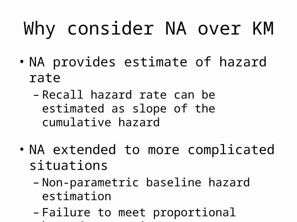
Why consider NA over KM
• NA provides estimate of hazard rate– Recall hazard rate can be estimated as slope of the
cumulative hazard
• NA extended to more complicated situations– Non-parametric baseline hazard estimation– Failure to meet proportional hazard assumption

Kernel Smoothing
• NA estimator of H(t) provides efficient estimate of cumulative hazard function
• More often interested in hazard rate h(t)
• Slope of H(t) provides crude estimate of h(t)
• Can use kernel smoothing based on H(t) and var(H(t)) to get this estimate of h(t)
0lim t
P t T t t T th t
t

Kernel Smoothing
• Recall the NA estimate:
• Crude hazard rate estimate:
• Can take advantage of the weighted average of crude estimates over event times close to t
• “Closeness” determined by bandwidth b• Average estimates over (t – b, t + b)
1
10 if
ifi
i
i t
dY
t
t tH t t t
dH th t
dt

Kernel Smoothed HR Estimator
• HR estimator
• t > b (greater than bandwidth)• A pointwise CI for the smoothed hazard rate is
constructed similarly as for the hazard rate
1
1
22 2
1
ˆ
ˆ ˆ
i
i
D t tibi
D t tibi
h t b K H t
h t b K V H t

Kernel Function
• Controls weights of nearby points• K(x) simplest class are symmetric PDFs with
• The most common choice are kernels defined on [-1,1] and are polynomial functions related to the beta distribution
1. 0
2. 0 0
3. 1
K x
xK x dx E K x
K x dx

Kernel Function
• Examples:– Rectangle (uniform)
– Epanechnikov
– Biquadratic (Biweight)
– Triquadratic
12
234
221516
323532
, 1 1
1 , 1 1
1 , 1 1
1 , 1 1
K x x
K x x x
K x x x
K x x x


A Few More Notes on Kernel Functions
• Issues with symmetric kernels– When b > t, symmetric kernels are no longer valid
since there are no event times less than 0
• Occurs at the left part of the graph• There are suggested modified kernels
– When data are sparse, the variability of the kernel estimator is large and results can be quite biased
• There are boundary corrections that can be applied

Choice of Bandwidth
• May chose to get desired smoothness of H(t)• May choose to minimize some criteria – For example MSE
• May choose using cross-validation – Computationally intensive
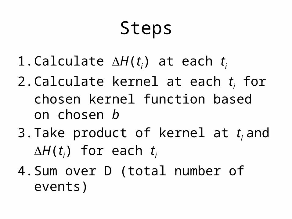
Steps
1. Calculate DH(ti) at each ti
2. Calculate kernel at each ti for chosen kernel function based on chosen b
3. Take product of kernel at ti and DH(ti) for each ti
4. Sum over D (total number of events)

Bone Marrow Transplant for Leukemia
• Patient undergoing bone marrow transplant (BMT) for acute leukemia
• Three types of leukemia– ALL– AML low risk– AML high risk
• We’re focusing on the ALL patients (first 10 events only)
• Using the Epanechnikov kernel

Bone Marrow Transplant for Leukemia
• Focusing on the ALL patients (first 10 events only)
• Using the Epanechnikov kernel• Bandwidth of 50• Want to estimate hazard rate at 75 weeks:
11
ˆ iD t t
ib bih t K H t

Time (ti)
1 0.0263
55 0.0533
74 0.0811
86 0.1097
104 0.1391
107 0.1694
109 0.2007
110 0.2329
122 0.2996
129 0.3353
H t 7550
it H t 7550
itK

Potential Issues
• Choice of bandwidth– How to select appropriate band width– N used to estimate hazard decreases as t increases
• Unexpected noise at later time points
• Tail Problem– Prefer symmetric kernels that integrate to 1 over support [-
1,1]– All observations s within the same distance from t are
weighted the same (i.e. in interval [t – b, t + b])– Problem if t < b or t > Tmax - b

Selection of Bandwidth
• Magnitude– Small Bandwidth
• less smooth curve and larger variance but small bias
– Larger bandwidth• Smoother and smaller variance but more bias
• Choice most crucial (influential) near boundary
1
!
211 1
ˆ 1 where
ˆ 1
kk k k
k k k
h t
nb F t G t
bias h t b h t B o B x K x dx
Var h t K x dx o

Selection of Bandwidth
• Global bandwidth– Constant bandwidth across all t– Chosen for simplicity– Optimized by:
– Problematic towards right tail (variance HUGE)
2
2
0
ˆ
ˆ ˆvar
ˆ arg min
t
b
IMSE b E h x h x dx
h x bias h x dx
b IMSE b
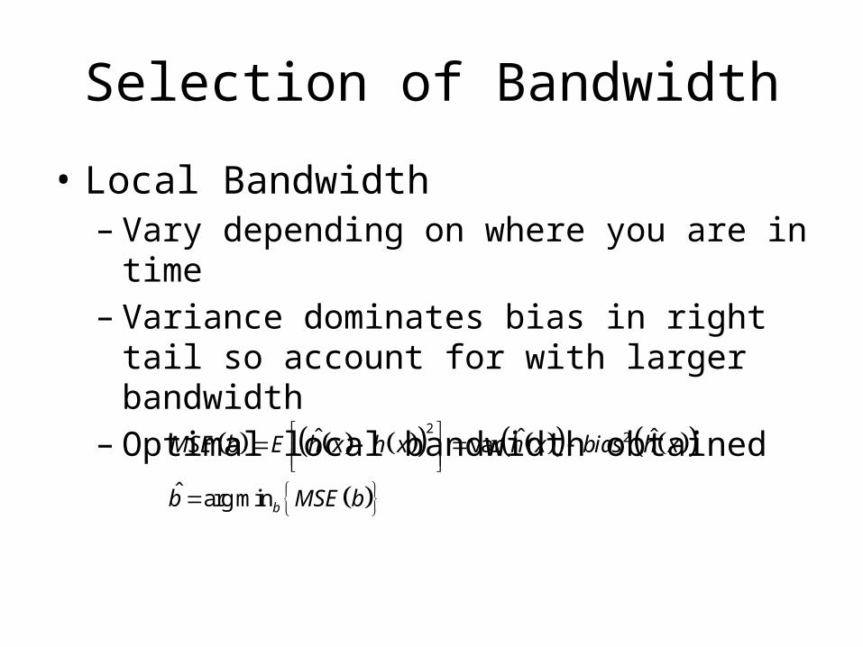
Selection of Bandwidth
• Local Bandwidth – Vary depending on where you are in time– Variance dominates bias in right tail so account for
with larger bandwidth– Optimal local bandwidth obtained
22ˆ ˆ ˆvar
ˆ arg minb
MSE b E h x h x h x bias h x
b MSE b
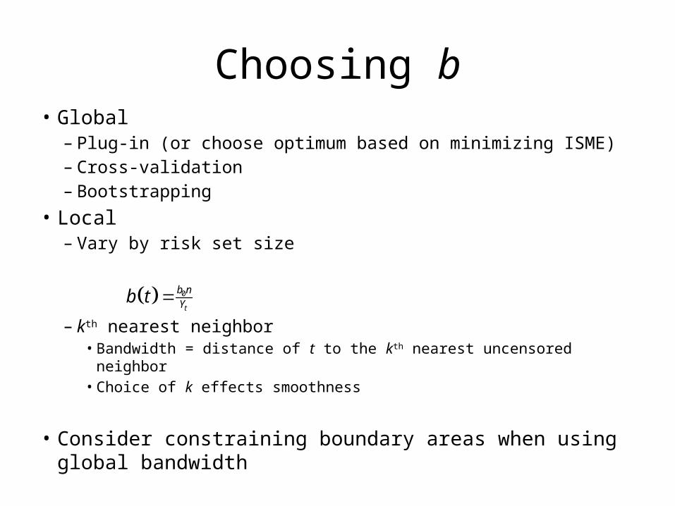
Choosing b• Global
– Plug-in (or choose optimum based on minimizing ISME)– Cross-validation– Bootstrapping
• Local– Vary by risk set size
– kth nearest neighbor• Bandwidth = distance of t to the kth nearest uncensored neighbor• Choice of k effects smoothness
• Consider constraining boundary areas when using global bandwidth
0
t
b nYb t

R Package “muhaz”• Function: muhaz– Estimate hazard function from right-censored data
using kernel-based methods
• Options – 3 bandwidth functions
• Global, local, kth nearest neighbor
– 3 types of boundary correction• None, left, both
– 4 four shapes kernel function• Rectangle, epanechnikov, biquadratic, triquadratic
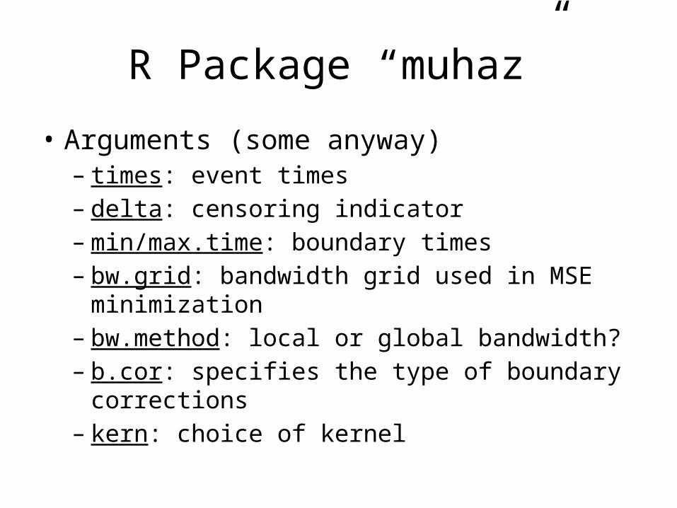
R Package “muhaz”
• Arguments (some anyway)– times: event times– delta: censoring indicator– min/max.time: boundary times– bw.grid: bandwidth grid used in MSE minimization– bw.method: local or global bandwidth?– b.cor: specifies the type of boundary corrections– kern: choice of kernel
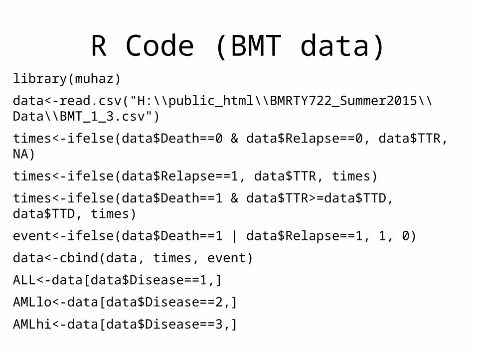
R Code (BMT data)library(muhaz)
data<-read.csv("H:\\public_html\\BMRTY722_Summer2015\\Data\\BMT_1_3.csv")
times<-ifelse(data$Death==0 & data$Relapse==0, data$TTR, NA)
times<-ifelse(data$Relapse==1, data$TTR, times)
times<-ifelse(data$Death==1 & data$TTR>=data$TTD, data$TTD, times)
event<-ifelse(data$Death==1 | data$Relapse==1, 1, 0)
data<-cbind(data, times, event)
ALL<-data[data$Disease==1,]
AMLlo<-data[data$Disease==2,]
AMLhi<-data[data$Disease==3,]

R Code (Comparing Kernels)### Comparing Kernel functions with set bandwidthALLe<-muhaz(ALL$times/365, ALL$event, bw.grid=0.33)ALLr<-muhaz(ALL$times/365, ALL$event, bw.grid=0.33, kern="r")ALLb<-muhaz(ALL$times/365, ALL$event, bw.grid=0.33, kern="b")ALLt<-muhaz(ALL$times/365, ALL$event, bw.grid=0.33, kern="t")
par(cex.axis=0.8)plot(ALLr, lty=1, lwd=2, col=1, xlab="Time to Relapse or Death (Years)",
ylab="Estimated Hazard Rate", xlim=c(0, 2), ylim=c(0, 1))lines(ALLe, lty=3, lwd=2, col=2)lines(ALLb, lty=2, lwd=2, col=3)lines(ALLt, lty=4, lwd=2, col=4)legend(1.5, 1, c("Rectangular","Epanechnikov", "Biweight","Triquadratic"),
col=1:4, lty=c(1,3,2,4), lwd=2, cex=0.8, bty="n")
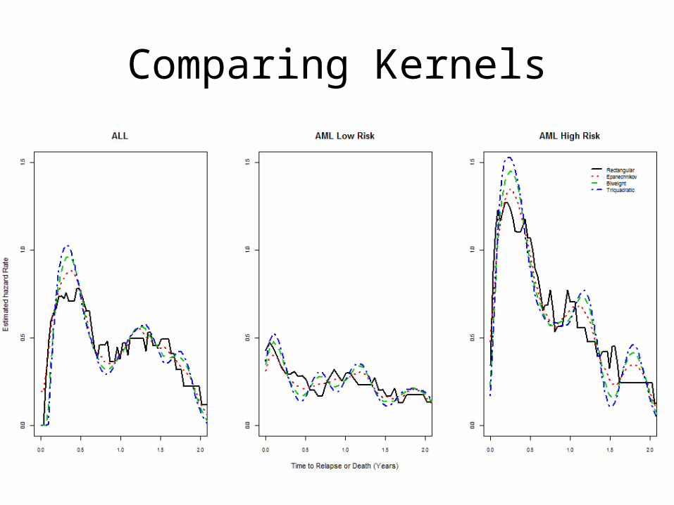
Comparing Kernels

R Code (Comparing global bandwidth)### Comparing different set global bandwidthALLe1<-muhaz(ALL$times/365, ALL$event, bw.grid=0.25)ALLe2<-muhaz(ALL$times/365, ALL$event, bw.grid=0.5)ALLe3<-muhaz(ALL$times/365, ALL$event, bw.grid=1)ALLe4<-muhaz(ALL$times/365, ALL$event, bw.method="global")
plot(ALLe1, lty=1, lwd=2, col=1, xlab="Time to Relapse or Death (Years)", ylab="Estimated Hazard Rate", xlim=c(0, 2), ylim=c(0, 1))
lines(ALLe2, lty=3, lwd=2, col=2)lines(ALLe3, lty=2, lwd=2, col=3)lines(ALLe4, lty=4, lwd=2, col=4)legend(1.5, 1, c("Rectangular","Epanechnikov", "Biweight","Triquadratic"),
col=1:4, lty=c(1,3,2,4), lwd=2, cex=0.8, bty="n")

Comparing Global Bandwidths

R Code (bandwidth methods)### Comparing different set global bandwidthALLe1<-muhaz(ALL$times/365, ALL$event, bw.grid=0.25)ALLe2<-muhaz(ALL$times/365, ALL$event, bw.grid=0.5)ALLe3<-muhaz(ALL$times/365, ALL$event, bw.grid=1)ALLe4<-muhaz(ALL$times/365, ALL$event, bw.method="global")
plot(ALLe1, lty=1, lwd=2, col=1, xlab="Time to Relapse or Death (Years)", ylab="Estimated Hazard Rate", xlim=c(0, 2), ylim=c(0, 1))
lines(ALLe2, lty=3, lwd=2, col=2)lines(ALLe3, lty=2, lwd=2, col=3)lines(ALLe4, lty=4, lwd=2, col=4)legend(1.5, 1, c("Rectangular","Epanechnikov", "Biweight","Triquadratic"),
col=1:4, lty=c(1,3,2,4), lwd=2, cex=0.8, bty="n")

Comparing Bandwidth Methods

Alternatively…
Smoothing Splines
• Alternative way to estimate the smooth hazard function is via smoothing splines
• But first, a basic discussion of smoothing splines

Motivation for Splines
• Why use smoothing splines in any kind of modeling
• Though we often treat relationships as linear, this is not generally reality– Convenient and easy to interpret– May be a reasonable under constraints– Sometimes necessary
• Large p, small N (avoid overfitting)
• Sometimes however, it makes sense to move beyond linearity

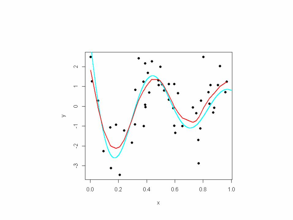
Motivation

Motivation

Motivation

Linear Basis Expansion• Linear Regression
– Question: How do you find ?
x1 x2 x3 y
1 -3 6 12
… … … …
1 1 2 2 3 3Truth: Y f x X X X
f̂ x

Linear Basis Expansion• Non-linear Model
– Question: Now how do you find ?
x1 x2 x3 y
1 3 6 12
… … … …
f̂ x
3 21 1 2 2 2 3 3 4 1Truth: sinXY X X X e X X

Linear Basis Expansion
• Non-linear model
• Apply linear regression to obtain
x1 x2 x3 u1 u2 u3 u4 y
1 -3 6 3 1201 0.052 1 12
… … … … … … … …
1 1 2 2 3 3 4 4Truth: Y U U U U
1 2 3 4ˆ ˆ ˆ ˆ, , ,
Linear Basis Expansion
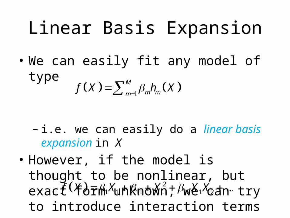
• We can easily fit any model of type
– i.e. we can easily do a linear basis expansion in X• However, if the model is thought to be
nonlinear, but exact form unknown, we can try to introduce interaction terms
1
M
m mmf X h X
21 1 11 1 12 1 2 ...f X X X X X

Piecewise Polynomial Functions
• Assume X is one-dimensional
• Definition: Assume the domain [a, b] of X is split into intervals [a, x1], [x2, x3],…, [a, xm, b]. Then f (X) is said to be a piecewise polynomial if f (X) is represented by separate polynomials in the different intervals. The points x1, x2, …, xm are called knots
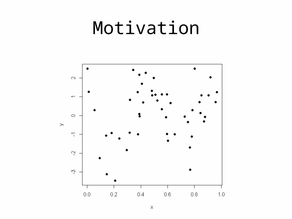
Motivation

Piecewise Polynomials

Piecewise Polynomials with Constraints
• For a continuous piecewise linear function we need to add constraints…– linear functions on each interval with constraints

With Constraints

Splines
• A piecewise polynomial is called an order-M spline if it has continuous derivatives up to order M-1
• Can be represented by a basis function (K = # knots)
• 4th order spline is called a cubic spline• Note, in cubic splines, knot-discontinuity is not visible
1
1
, 1, 2,...,
, 1, 2,...,
jj
M
M l l
h X X j M
h X X l K

Cubic Splines
• Given a < x1 < x2 < … < xn < b, a function h is
a cubic spline if1. On each interval (a , x1), (x1, x2), …, (xn,b), h is a
cubic polynomial
2. The polynomial pieces fit together at points xi
(knots) s.t. h itself and its first and second derivatives are continuous at each xi, and hence
on the whole [a,b]

Natural Cubic Splines
• A cubic spline f is called a natural cubic spline if its 2nd and 3rd derivatives are 0 at a and b
• Implies that f is linear on extreme intervals

Fitting Smooth Functions to Data• Minimize a penalized sum of squared residuals
• The function f that minimizes RRS for a given l is a natural cubic spline with knots at all unique values of xi (Note- this means there are N knots)
2 2
1, "
N
i iiRSS f y f x f t dt
Where l is a smoothing parameter
l = 0: any function interpolating datal = +: least squares line fit
R Package “gss”
• R smoothing splines for hazard function
• Description: Estimate hazard function using smoothing spline ANOVA models. The symbolic model specification via formula follows the same rules as in lm, but with response of special form

“sshzd” Function• sshzd takes standard right-censored lifetime data, with possible left-truncation
and covariates; in Surv(futime,status,start=0)~..., futime is the follow-up time, status is the censoring indicator, and start is the optional left-truncation time. The main effect of futime must appear in the model terms specified via ....
• Parallel to those in a ssanova object, the model terms are sums of unpenalized and penalized terms. Attached to every penalized term there is a smoothing parameter, and the model complexity is largely determined by the number of smoothing parameters.
• The selection of smoothing parameters is through a cross-validation mechanism described in Gu (2002, Sec. 7.2), with a parameter alpha; alpha=1 is "unbiased" for the minimization of Kullback-Leibler loss but may yield severe undersmoothing, whereas larger alpha yields smoother estimates.
• A subset of the observations are selected as "knots." Unless specified via id.basis or nbasis, the number of "knots" q is determined by max(30,10n^{2/9}), which is appropriate for the default cubic splines for numerical vectors.

Marrow Transplant### Smoothed hazardsdata<-read.csv("H:\\BMTRY_722_Summer2013\\BMT_1_3.csv")times<-ifelse(data$Death==0 & data$Relapse==0, data$TTR, NA)times<-ifelse(data$Relapse==1, data$TTR, times)times<-ifelse(data$Death==1 & data$TTR>=data$TTD, data$TTD, times)event<-ifelse(data$Death==1 | data$Relapse==1, 1, 0)data<-cbind(data, times, event)
km.fit<-survfit(Surv(data$times, data$event)~data$Disease)h1<--log(km.fit$surv[1:37]); t1<-km.fit$time[1:37]h2<--log(km.fit$surv[38:91]); t2<-km.fit$time[38:91]h3<--log(km.fit$surv[92:135]); t3<-km.fit$time[92:135]
plot(t1, h1, xlab="Time", ylab="H(t)", xlim=c(0, 2640), ylim=c(0,1.5), type="s", col=1, lwd=2)lines(t2, h2, type="s", col=2, lwd=2)lines(t3, h3, type="s", col=3, lwd=2)legend(1750, .3, c("ALL","AML low","AML high"), col=1:3, lwd=2, cex=0.8)

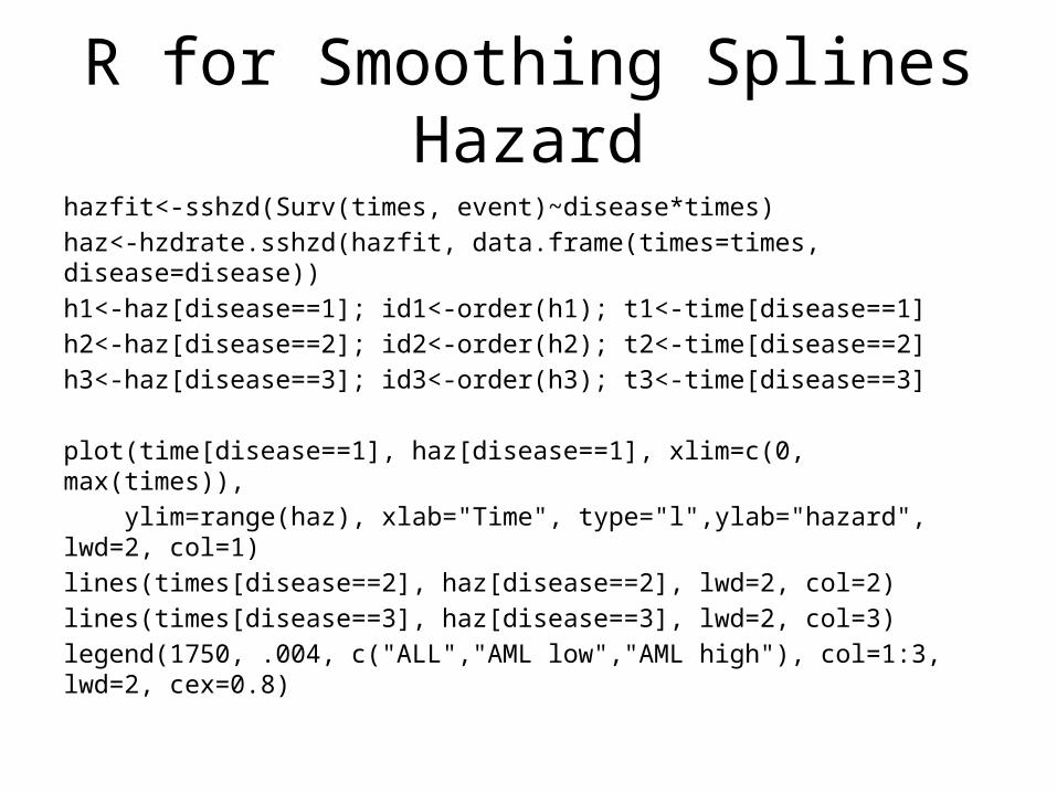
R for Smoothing Splines Hazardhazfit<-sshzd(Surv(times, event)~disease*times)haz<-hzdrate.sshzd(hazfit, data.frame(times=times, disease=disease))h1<-haz[disease==1]; id1<-order(h1); t1<-time[disease==1]h2<-haz[disease==2]; id2<-order(h2); t2<-time[disease==2]h3<-haz[disease==3]; id3<-order(h3); t3<-time[disease==3]
plot(time[disease==1], haz[disease==1], xlim=c(0, max(times)), ylim=range(haz), xlab="Time", type="l",ylab="hazard", lwd=2, col=1)lines(times[disease==2], haz[disease==2], lwd=2, col=2)lines(times[disease==3], haz[disease==3], lwd=2, col=3)legend(1750, .004, c("ALL","AML low","AML high"), col=1:3, lwd=2, cex=0.8)


Non-Intersecting Hazardshazfit<-sshzd(Surv(times, event)~disease+times)haz<-hzdrate.sshzd(hazfit, data.frame(times=times, disease=disease))h1<-haz[disease==1]; id1<-order(h1); t1<-time[disease==1]h2<-haz[disease==2]; id2<-order(h2); t2<-time[disease==2]h3<-haz[disease==3]; id3<-order(h3); t3<-time[disease==3]
plot(time[disease==1], haz[disease==1], xlim=c(0, max(times)), ylim=range(haz), xlab="Time", type="l",ylab="hazard", lwd=2, col=1)lines(times[disease==2], haz[disease==2], lwd=2, col=2)lines(times[disease==3], haz[disease==3], lwd=2, col=3)legend(1750, .004, c("ALL","AML low","AML high"), col=1:3, lwd=2, cex=0.8)


