
1
EE462 MLCV
Lecture 13-14Face Recognition Subspace/Manifold Learning
Tae-Kyun Kim
EE462 MLCV
2
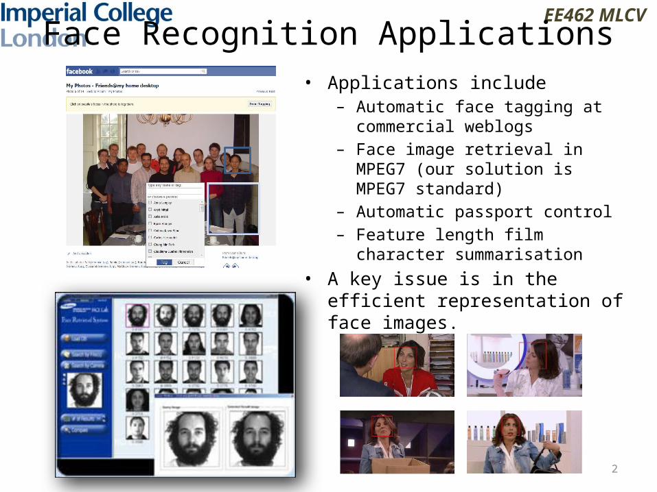
Face Recognition Applications• Applications include
– Automatic face tagging at commercial weblogs
– Face image retrieval in MPEG7 (our solution is MPEG7 standard)
– Automatic passport control– Feature length film character
summarisation
• A key issue is in the efficient representation of face images.

EE462 MLCV
3
Face image data sets
Object categorisation data sets
Intraclass variation
Interclass variation
Intraclass variation
Interclass variation
Class 1
Class 2 Class 1
Class 2
Face Recognition vs Object Categorisation
4
EE462 MLCV
In both, we try representations/features that minimise intraclass variations and maximise interclass variations.
Face image variations are more subtle, compared to those of generic object categories.
Subspace/manifold techniques, cf. Bag of Words, are dominating-arts for face image analysis.
Face Recognition vs Object Categorisation
5
EE462 MLCV
Principal Component Analysis (PCA)
Maximum Variance FormulationMinimum-error formulation
Probabilistic PCA
EE462 MLCV
6
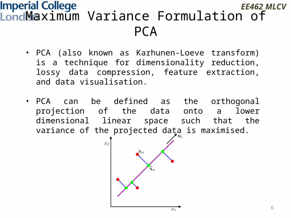
Maximum Variance Formulation of PCA
• PCA (also known as Karhunen-Loeve transform) is a technique for dimensionality reduction, lossy data compression, feature extraction, and data visualisation.
• PCA can be defined as the orthogonal projection of the data onto a lower dimensional linear space such that the variance of the projected data is maximised.
EE462 MLCV
7
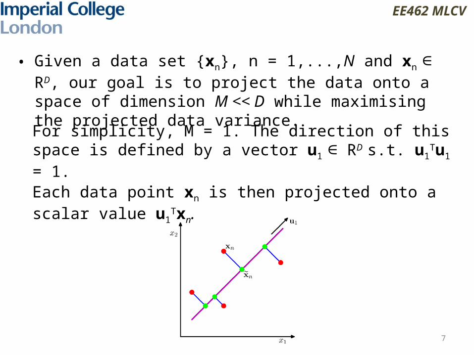
• Given a data set {xn}, n = 1,...,N and xn R∈ D, our goal is to project the data onto a space of dimension M << D while maximising the projected data variance.
For simplicity, M = 1. The direction of this space is defined by a vector u1 R∈ D s.t. u1
Tu1 = 1.
Each data point xn is then projected onto a scalar value u1Txn.
EE462 MLCV
8
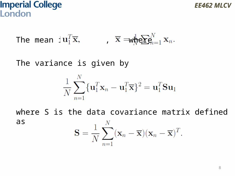
The mean is , where
The variance is given by
where S is the data covariance matrix defined as

EE462 MLCV
9
We maximise the projected variance u1TSu1 with respect to
u1 with the normalisation condition u1Tu1 = 1.
The Lagrange multiplier formulation is
By setting the derivative with respect to u1 to zeros, we obtain
u1 is an eigenvector of S.
By multiplying u1T , the variance is obtained by

EE462 MLCV
10
𝐮1
The variance is a maximum when u1 is the eigenvector with the largest eigenvalue λ1.
The eigenvector is called the principal component.
For the general case of an M dimensional subspace, it is obtained by the M eigenvectors u1, u2, … , uM of the data covariance matrix S corresponding to the M largest eigenvalues λ1, λ2 …, λM.
0, otherwise𝐮2
EE462 MLCV
11
Minimum-error formulation of PCA
0, otherwise
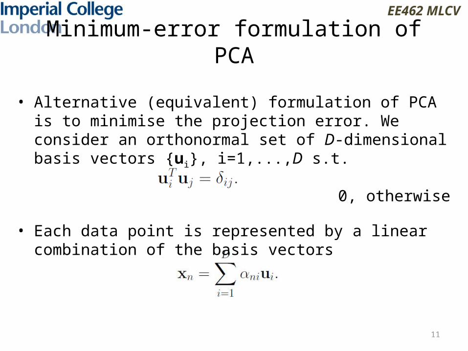
• Alternative (equivalent) formulation of PCA is to minimise the projection error. We consider an orthonormal set of D-dimensional basis vectors {ui}, i=1,...,D s.t.
• Each data point is represented by a linear combination of the basis vectors
EE462 MLCV
12
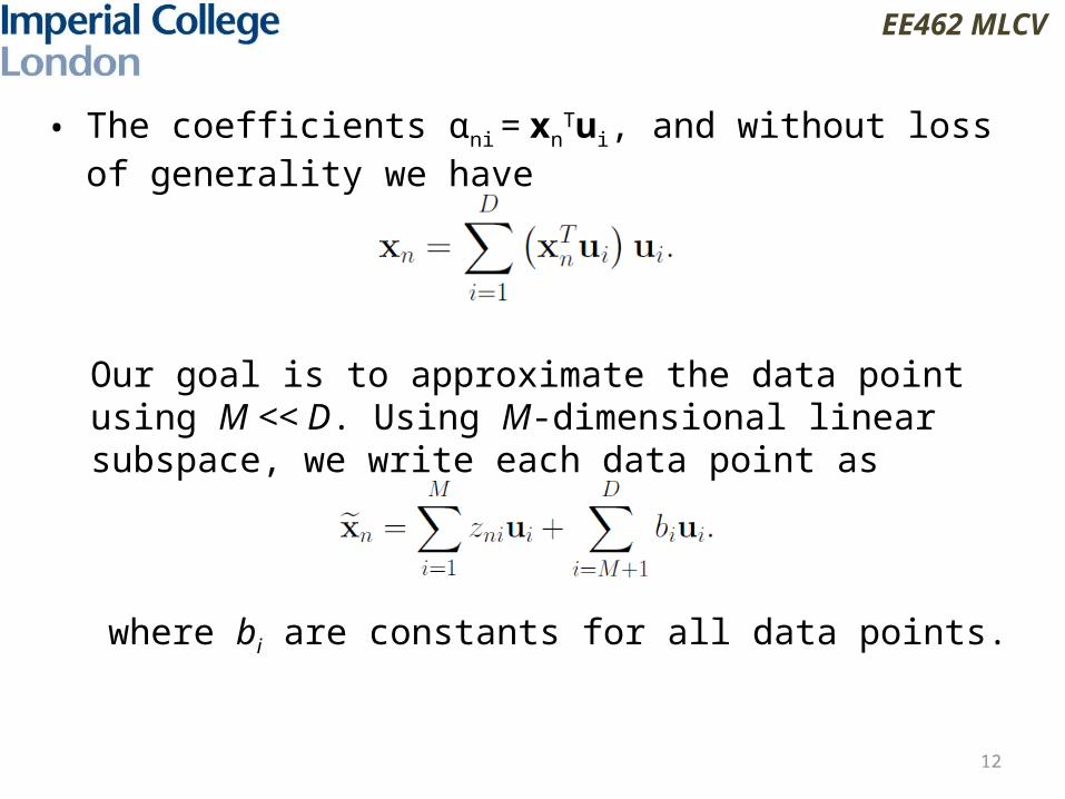
• The coefficients αni = xnTui, and without loss of generality we
have
Our goal is to approximate the data point using M << D. Using M-dimensional linear subspace, we write each data point as
where bi are constants for all data points.
EE462 MLCV
13
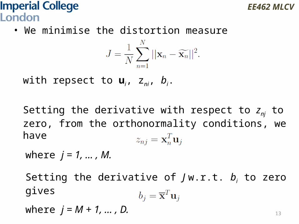
• We minimise the distortion measure
with repsect to ui, zni, bi.
Setting the derivative with respect to znj to zero, from the orthonormality conditions, we have
where j = 1, … , M.
Setting the derivative of J w.r.t. bi to zero gives
where j = M + 1, … , D.
EE462 MLCV
14
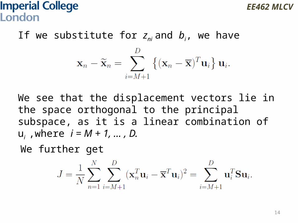
If we substitute for zni and bi, we have
We see that the displacement vectors lie in the space orthogonal to the principal subspace, as it is a linear combination of ui ,where i = M + 1, … , D.
We further get

EE462 MLCV
15
• Consider a two-dimensional data space D = 2 and a one-dimensional principal subspace M = 1. Then, we choose u2 that minimises
Setting the derivative w.r.t. u2 to zeros yields Su2 = λ2u2
We therefore obtain the minimum value of J by choosing u2 as the eigenvector corresponding to the smaller eigenvalue. We choose the principal subspace by the eigenvector with the larger eigenvalue.

EE462 MLCV
16
• The general solution is to choose the eigenvectors of the covariance matrix with M largest eigenvalues.
where I = 1, ... ,M.
The distortion measure becomes

17
EE462 MLCV
Applications of PCA to Face Recognition
EE462 MLCV
18
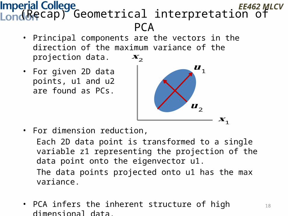
(Recap) Geometrical interpretation of PCA
• Principal components are the vectors in the direction of the maximum variance of the projection data.
• For dimension reduction,
Each 2D data point is transformed to a single variable z1 representing the projection of the data point onto the eigenvector u1.
The data points projected onto u1 has the max variance.
• PCA infers the inherent structure of high dimensional data.• The intrinsic dimensionality of data is much smaller.
• For given 2D data points, u1 and u2 are found as PCs.
𝐮1
𝐮2
𝐱1
𝐱 2

EE462 MLCV
19
Eigenfaces• Collect a set of face images.• Normalize for scale, orientation, location (using eye locations), and
vectorise them.
• Construct the covariance
matrix S and obtain eigenvectors U.
w
h
,......,,1
xxXXXN
S iT
MDRUUSU ,
D=wh
NDRX
M: number of eigenvectors
N: number of images

EE462 MLCV
20
Eigenfaces• Project data onto the
subspace
• Reconstruction is obtained as
• Use the distance to the subspace for face recognition
DMRZXUZ NMT ,,
UZXUzuzxM
iii
~,~
1
x~||~|| xx
x
EE462 MLCV
21
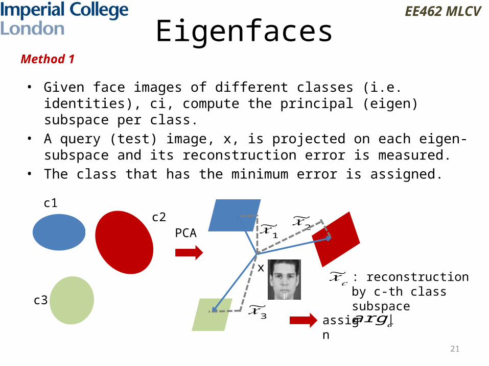
Eigenfaces
c1
c3
c2
arg𝑐|assign
~𝑥𝑐 : reconstruction by c-th class subspace
Method 1
• Given face images of different classes (i.e. identities), ci, compute the principal (eigen) subspace per class.
• A query (test) image, x, is projected on each eigen-subspace and its reconstruction error is measured.
• The class that has the minimum error is assigned.
PCA
x
~𝑥1~𝑥2
~𝑥3

EE462 MLCV
22
Eigenfaces
c1
c3
c2 x
|arg𝑐assign
𝑧𝑐: projection of c-th class data mean
PCA
Method 2
• Given face images of different classes (i.e. identities), ci, compute the principal (eigen) subspace over all data.
• A query (test) image, x, is projected on the eigen-subspace and its projection, z, is compared with the projections of the class means.
• The class that has the minimum error is assigned.
𝑧1𝑧 2
𝑧 3
𝑧
23
EE462 MLCV
Matlab Demos Face Recognition by PCA
• Face Images• Eigenvectors and Eigenvalue plot• Face image reconstruction• Projection coefficients (visualisation of high-dimensional
data)• Face recognition

EE462 MLCV
24
Probabilistic PCA (PPCA)
• A subspace is spanned by the orthonormal basis (eigenvectors computed from covariance matrix).
• It interprets each observation with a generative model.
• It estimates the probability of generating each observation with Gaussian distribution,
PCA: uniform prior on the subspace
PPCA: Gaussian dist. on the subspace
EE462 MLCV
25
Continuous Latent Variable Model
• PPCA has a continuous latent variable. • GMM (mixture of Gaussians) is the model with a discrete
latent variable.
• PPCA represents that the original data points lie close to a manifold of much lower dimensionality.
• In practice, the data points will not be confined precisely to a smooth low-dimensional manifold. We interpret the departures of data points from the manifold as noise.
Lecture 3-4

EE462 MLCV
26
• Consider an example of digit images that undergo a random displacement and rotation.
• The images have the size of 100 x 100 pixel values, but the degree of freedom of variability across images is only three: vertical, horizontal translations and rotations.
• The data points live on a subspace whose intrinsic dimensionality is three.
• The translation and rotation parameters are continuous latent (hidden) variables. We only observe the image vectors.
Continuous Latent Variable Model

EE462 MLCV
27
Probabilistic PCA• PPCA is an example of the linear-Gaussian framework, in which
all marginal and conditional distributions are Gaussian.
• We define a Gaussian prior distribution over the latent variable z as
The observed D dimensional variable x is defined as
where z is an M dimensional Gaussian latent variable, W is the D x M matrix and ε is a D dimensional zero-mean Gaussian-distributed noise variable with covariance σ2I.
Lecture 15-16
EE462 MLCV
28
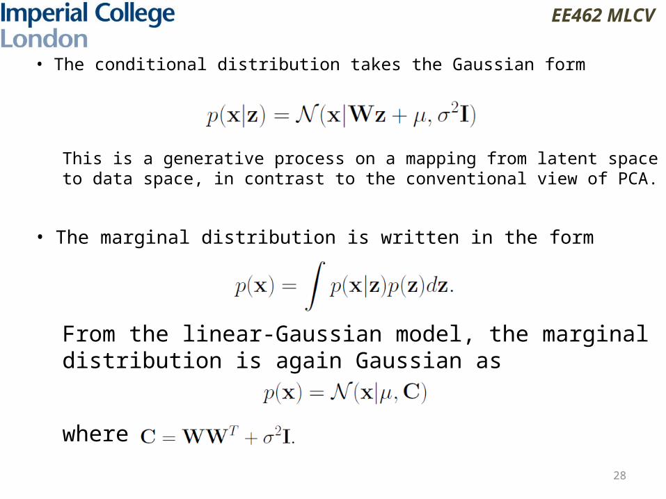
• The conditional distribution takes the Gaussian form
This is a generative process on a mapping from latent space to data space, in contrast to the conventional view of PCA.
• The marginal distribution is written in the form
From the linear-Gaussian model, the marginal distribution is again Gaussian as
where

EE462 MLCV
29
The above can be seen from

EE462 MLCV
30
EE462 MLCV
31
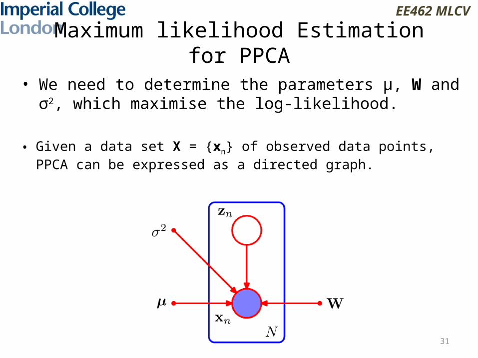
Maximum likelihood Estimation for PPCA
• We need to determine the parameters μ, W and σ2, which maximise the log-likelihood.
• Given a data set X = {xn} of observed data points, PPCA can be expressed as a directed graph.

EE462 MLCV
32
The log likelihood is
For detailed optimisations, see Tipping and Bishop, PPCA (1999).
where UM is the D x M eigenvector matrix of S, and LM is the M x M diagonal eigenvalue matrix, R is an orthogonal rotation matrix s.t. RRT= I.

EE462 MLCV
33
Hence, it is independent of R.
Redundancy happens up to rotations, R, of the latent space coordinates.
Consider a matrix where R is an orthogonal rotation matrix s.t. RRT= I. We see

EE462 MLCV
34
• Conventional PCA is generally formulated as a projection of points from the D dimensional data space onto an M dimensional linear subspace.
• PPCA is most naturally expressed as a mapping from the latent space to the data space.
• We can reverse this mapping using Bayes' theorem to get the posterior distribution p(z|x) as
where the M x M matrix M is defined by
35
EE462 MLCV
Limitations of PCA

EE462 MLCV
36
Unsupervised learning
PCA vs LDA
PCA finds the direction for maximum variance of data (unsupervised), while LDA (Linear Discriminant Analysis) finds the direction that optimally separates data of different classes (supervised).
EE462 MLCV
37
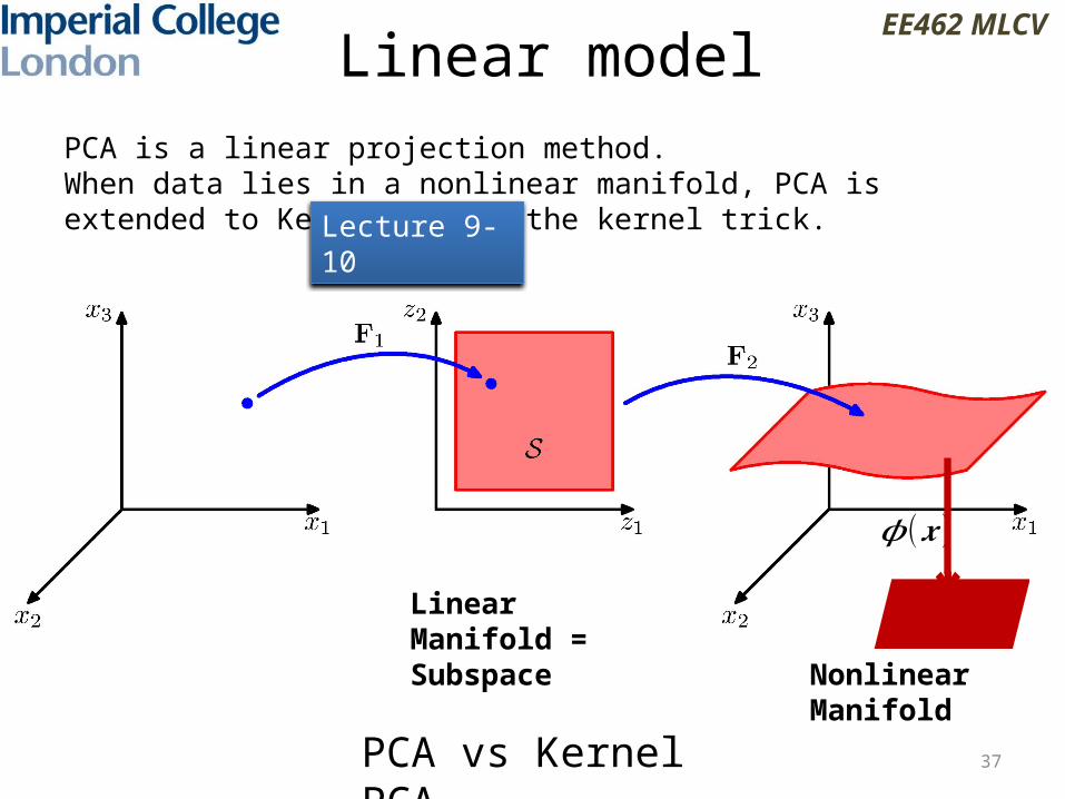
Linear model
Linear Manifold = Subspace Nonlinear
Manifold
PCA vs Kernel PCA
PCA is a linear projection method. When data lies in a nonlinear manifold, PCA is extended to Kernel PCA by the kernel trick.
𝝓(𝒙 )
Lecture 9-10
EE462 MLCV
38
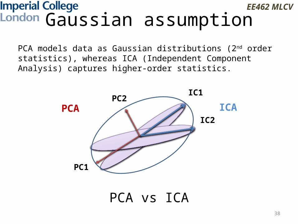
Gaussian assumption
IC1
IC2
PC1
PC2
PCA vs ICA
PCA models data as Gaussian distributions (2nd order statistics), whereas ICA (Independent Component Analysis) captures higher-order statistics.
PCA ICA
EE462 MLCV
39
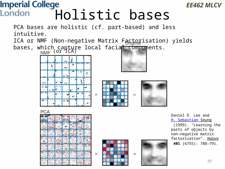
(or ICA)
PCA bases are holistic (cf. part-based) and less intuitive. ICA or NMF (Non-negative Matrix Factorisation) yields bases, which capture local facial components.
Daniel D. Lee and H. Sebastian Seung (1999). "Learning the parts of objects by non-negative matrix factorization". Nature 401 (6755): 788–791.
Holistic bases


