
LASER INDUCED BREAKDOWN SPECTROSCOPIC ANALYSIS OF METAL
AEROSOLS GENERATED BY PNEUMATIC NEBULIZATION OF AQUEOUS SOLUTIONS
A Thesis Submitted to the Graduate School of Engineering and Sciences of
İzmir Institute of Technology in Partial Fulfillment of the Requirements for the Degree of
MASTER OF SCIENCE
in Chemistry
by Dilek ARICA ATEŞ
JULY 2010 İZMİR

We approve the thesis of Dilek ARICA ATEŞ __________________________________ Assoc. Prof. Dr. Şerife YALÇIN Supervisor __________________________________ Prof Dr. Hürriyet POLAT Committee Member __________________________________ Assist. Prof. Dr. Enver TARHAN Committee Member 1 July 2010 ________________________________ _____________________________ Prof. Dr. Serdar ÖZÇELİK Assoc. Prof. Dr. Talat YALÇIN Head of the Department of Chemistry Dean of the Graduate School of
ii
Engineering and Sciences

ACKNOWLEDGMENTS
I would like thank to several people who really helped and supported me through
out my thesis studies.
First of all, I would like to thank to Assoc. Prof. Dr. Şerife YALÇIN for her
generous supervising through out the time that we were working.
Besides, I would like to show my great appreciation to Prof. Dr. Hürriyet
POLAT for her valuable comments and great effort on particle size measurements. I
would like to thank to Assist. Prof. Dr Enver Tarhan for his valuable comments.
Also, I would like to thank to my laboratory mates Semira ÜNAL and Nadir
ARAS for their great friendship, help and for the enjoyable times we had together.
Nevertheless, I would like to mention my room mates Ezel BOYACI and Meral
KARACA and Ayşegül ŞEKER for their companian, and especially to Esen
DÖNERTAŞ, Merve DEMİRKURT, Hüseyin İLGÜ. They were the shining colors of
my days. Also, Elif Bilge KAVUN has been a great companion for many years. Her
sincere opinions and act have put on great challenge on me. She is the only one to be
real sisters with.
We would like to give our appreciation to TÜBİTAK for the financial support
for this project. (TBAG-108T376).
Furthermore, I would like to thank to Selahattin ÇAKMAK from Ege University
Glass Workshop and Polat BULANIK for their great talent and patience on making the
glass wares we needed.
iii
Last but not least, I would like to thank to my friend, love, and husband, “my
everything” Atilla ATEŞ for his valuable love and encouragement for completion of my
thesis and overcoming my difficult days. Without him, life would not exist for me.

ABSTRACT LASER INDUCED BREAKDOWN SPECTROSCOPIC ANALYSIS OF
METAL AEROSOLS GENERATED BY PNEUMATIC NEBULIZATION OF AQUEOUS SOLUTIONS
Laser Induced Breakdown Spectroscopy, LIBS, is an analytical technique used
to determine the elemental composition of samples in all forms. In this study, an
experimental LIBS system has been designed and constructed for the analysis of metal
aerosol particles that are generated by a pneumatic nebulizer. This research provides a
basis and preliminary data for the construction of a portable LIBS system to analyze
metals in aqueous environments.
The aerosol particles generated from the pneumatic nebulizer travel through a
sample introduction unit to reach the sample cell in which they interact with the laser
beam. The source of light is a Nd:YAG laser at 532 nm, 10 Hz. When the laser beam is
focused inside the sample cell, plasma is generated, and the emission containing the
spectral information about the sample being analyzed is focused onto the spectrograph
and detected by a gated detector. The optimum optical and experimental parameters
were systematically investigated.
The aqueous analyte solutions were prepared from their salts before introduced
into the system. In this work, laser-induced breakdown spectroscopic emissions of Na,
Ca, Mg and K aerosols were studied. In single shot mode, the minimum detectable
aqueous concentrations were found as 250 ppb, 500 ppb, 400 ppb and 10 mg/L
respectively. For 10 shot accumulated analyses in repetitive mode, based on 3
criterion, the detection limit (LOD) was determined as 1 mg/L, 0.6 mg/L, 1.5 mg/L and
16.3 mg/L respectively. The efficiency of the drying unit has been evaluated by particle
size measurements. It has been shown that the Na aerosols with particle size of 4.3 m
decreases to 0.5 m after passing through the membrane dryer unit.
iv

ÖZET
PNÖMATİK NEBULİZASYON METODU İLE SULU ÇÖZELTİLERDEN OLUŞTURULAN METAL AEROSOLLERİNİN
LAZER OLUŞTURMALI PLAZMA SPEKTROSKOPİSİ İLE ANALİZİ
Lazer Oluşturmalı Plazma Spektroskopisi, LIBS, katı, sıvı, gaz örneklerin
elemental bileşimlerinin belirlenmesinde kullanılan bir analitik metoddur. Bu tez
çalışmasında, pnömatik sisleştirici tarafından üretilen aerosollerin analizi için bir LIBS
düzeneği tasarlanmış ve kurulmuştur. Sisleştirici tarafından oluşturulan aerosol
parçacıkları ısıtma/soğutma bölümü ve membran kurutucudan geçerek örnek hücresine
ulaşmaktadır. Bu örnek hücresinde, parçacıklar ile lazer ışınının etkileşimi gerçekleşir.
Işık kaynağı olarak 532 nm ve 10 Hz’de pulslu ışık veren Nd:YAG kristalli lazer
kullanılmaktadır. Bu pulslu ışın, uygun optik malzemeler ile örnek hücresine odaklanır
ve plazma oluşturulur. Oluşan plazma emisyonu spektrograf ve dedektör üzerine
düşürülür ve spektal görüntü kaydedilir. Bu spektral dağılım, örnek hakkında bilgiler
içermektedir.
Analit çözeltiler, katı metal tuzlarından hazırlanarak sisteme verilmiştir. Bu
çalışmada, Na, Ca, Mg ve K elementlerinden elde edilen aerosollerin spektral
emisyonları incelenmiştir. Tek vuruşlu analizlerde tayin edilebilir en düşük sulu çözelti
konsantrasyonları sırasıyla 250 ppb, 500 ppb, 400 ppb and 10 ppm olarak bulunmuştur.
Tekrarlamalı modda 10 vuruş toplandığı analizlerde ise tayin limiti 1 mg/L, 0.6 mg/L,
1.5 mg/L ve 16.3 mg/L olarak bulunmuştur.
Bunun yanısıra, kurutma bölümünün verimini değerlendirmek amacıyla parçacık
ölçümleri gerçekleştirilmiştir. Sodyum aerosollerinin ısıtma/soğutma ve membran
kurutucu bölümlerinden geçtikten sonra parçacık boyutunun 4.3 m’den 0.5 m’ye
düştüğü görülmüştür.
v

TABLE OF CONTENTS
LIST OF FIGURES .......................................................................................................viii
LIST OF TABLES............................................................................................................ x
CHAPTER 1. INTRODUCTION ..................................................................................... 1
1.1. ..................................................................................................... 1 Subject
1.2. Introduction to Laser Induced Breakdown Spectroscopy, LIBS ............. 1
1.3. Local Thermodynamic Equilibrium......................................................... 2
1.4. Advantages and Disadvantages of LIBS ................................................. 3
1.5. Instrumentation ........................................................................................ 4
1.5.1. Lasers ................................................................................................. 6
1.5.2. Optic Materials .................................................................................. 8
1.6. LIBS on Liquid Samples Analysis........................................................... 9
1.6.1. Direct Liquid Analysis....................................................................... 9
1.6.2. Double Pulse LIBS .......................................................................... 11
1.6.3. LIBS on Aerosol Samples................................................................ 11
1.7. Aim of the Study.................................................................................... 14
CHAPTER 2. EXPERIMENTAL................................................................................... 16
2.1. LIBS Experimental Set-up..................................................................... 16
2.1.1. Aerosol Generation .......................................................................... 16
2.1.2. Desolvation of the Aerosols............................................................. 17
2.1.2.2. Membrane Drying...................................................................... 18
2.2. Instrumental ........................................................................................... 18
2.2.1. Detection System ............................................................................. 22
2.3. Reagents................................................................................................. 22
2.4. Aerosol Size Measurements................................................................... 22
CHAPTER 3. RESULTS AND DISCUSSION.............................................................. 24
3.1. Experimental Parameters ....................................................................... 24
3.1.1. Effect of Sample Flow Rate on Signal Intensity.............................. 24
3.1.2. Drying Gas Flow Rate ..................................................................... 26
3.2. Instrumental Parameters ........................................................................ 27
vi

3.2.1. Effect of Laser Pulse Energy on Signal Intensity ............................ 27
3.2.2. Time Resolution............................................................................... 30
3.2.3. Detector Gain................................................................................... 32
3.3. Qualitative Analysis............................................................................... 33
3.3.1. Representative Spectra..................................................................... 33
3.3.2. Effect of Membrane Dryer on H- Line ......................................... 38
3.3.4. Effect of Dessicant Prior to Membrane Dryer ................................. 39
3.4. Quantitative Analysis............................................................................. 40
3.4.1. Detection Limits .............................................................................. 43
3.4.2. Multi-element Analysis.................................................................... 44
3.4.3. Airborne Concentration ................................................................... 46
3.4.4. Particle Size ..................................................................................... 49
3.5. Spectral Temperature............................................................................. 50
CHAPTER 4. CONCLUSION ....................................................................................... 52
REFERENCES ............................................................................................................... 53
vii
LIST OF FIGURES
Figure Page
Figure 1.1. A typical LIBS set-up..................................................................................... 5
Figure 1.2. LIBS set-up for liquids. Beam focused on surface of the liquid. ................... 5
Figure 1.3. Optical cavity. ................................................................................................ 6
Figure 1.4. A four level laser scheme. .............................................................................. 8
Figure 2.1. Medical used to convert aqueous solutions into aerosols............................. 16
Figure 2.2. The pictorial and schematic representation of heating/cooling unit............. 17
Figure 2.3. Horizontal (a) and telescopic (b) beam setup............................................... 20
Figure 2.4. The aerosol generation unit attached to the particle sizer. ........................... 23
Figure 3.1. Effect of gas flow rate on Na signal intensity .............................................. 25
Figure 3.2. The amount of aqueous sample solution converted to aerosols ................... 26
Figure 3.3. LIBS signal intensity variation of (a) Na(I), (b) Mg(I), (c) K(I).................. 28
Figure 3.4. Appearance of noise with increasing laser energy ....................................... 29
Figure 3.5. Time resolution for (a) Ca, (b) Na aerosols.................................................. 30
Figure 3.6. Spectra of early plasma.. .............................................................................. 32
Figure 3.7. Effect of gain on potassium aerosols............................................................ 33
Figure 3.8. Representative Na spectra for 100 ppm Na.................................................. 34
Figure 3.9. Representative Ca spectrum for 100 ppm Ca............................................... 35
Figure 3.10. Representative Mg spectrum for 100 ppm Mg........................................... 36
Figure 3.11. Representative K spectrum for 1000 ppm K .............................................. 37
Figure 3.12. The increase in intensity of Na(I) line when membrane dryer is used....... 38
Figure 3.13. The decrease in intensity of H line when membrane dryer is used. ........... 39
Figure 3.14. Calibration plot for calcium. ...................................................................... 41
Figure 3.15. Calibration plot for sodium ........................................................................ 42
Figure 3.16. Calibration plot for magnesium.................................................................. 42
Figure 3.17. Calibration plot for potassium ................................................................... 43
Figure 3.18. The effect of presence of Mg and Ca ions on the signal strength of Na
588.9 nm line. ............................................................................................ 45
Figure 3.19. Spectra of mineral water (diluted 20 times) ............................................... 47
Figure 3.20. Spectra of tap water.................................................................................... 48
viii
Figure 3.21. Particle size distribution plots for Na……………………………………..50
Figure 3.22. The spectral temperature calculation for N(I) lines...……………………51
ix

x
LIST OF TABLES
Table Page
Table 1.1. Detection limits from literature. .................................................................... 15
Table 2.1. LIBS system specifications............................................................................ 21
Table 3.2. The icrease in peak area for Ca when a dessicant is placed .......................... 39
Table 3.4. Spectral emission lines of the elements studied. ........................................... 40
Table 3.5. The detection limits and minimum detectable solution concentrations......... 44
Table 3.6. Particle size measurements. ........................................................................... 49
CHAPTER 1
INTRODUCTION
1.1. Subject
Everyday the amount of pollutants and toxic compounds are becoming more
frequently used in industry and many other areas of work. In order to determine,
identify and control those pollutants and toxic materials, atomic spectroscopic
instruments like Atomic Absorption Spectroscopy, AAS, Inductively Coupled Plasma
Optical Emission Spectroscopy, ICP-OES are required and widely used. However, due
to long time of analyses the consumption rates of purge gasses and chemicals are high
for those methods. Even more, the process steps accompanied to those methods to
isolate the analyte may result as the loss of identity of the sample. Besides, all those
methods require time to bring the sample to the laboratory. On account of those reasons
described above, in order to save time and other expenses, a method should be
developed for fast and cheap analysis compared to those methods. Laser Induced
Breakdown technique provides many advantages such as no sample preparation and no
chemical solvent consumption. Also, LIBS technique can be applied on all types of
sample with high detection limits and precision of 5%. The benefits of the LIBS are
further discussed in following sections.
This thesis presents a study on the development of a compact prototype device
which can be used on field. The designed instrument is used for the analysis of several
elements. After the optimization of system parameters are performed, real samples are
introduced to the system.
1.2. Introduction to Laser Induced Breakdown Spectroscopy, LIBS
By the invention of lasers in 1960s, lasers have taken place in many areas of
research (Andrew 2006). One of the applications of the laser includes the Laser Induced
Breakdown Spectroscopy, shortly LIBS (Radziemski, Cremers, Wiley, 2006). LIBS is
an atomic emission spectroscopic technique which uses a pulsed laser to form plasma.
Plasma is considered to be a cloud of electrons and ions that results from the breakdown
1
of the sample. Laser plasma can be formed on any type of a sample: solid, liquid, gas
and aerosol. When a high power pulsed laser sent onto the sample, the sample absorbs
the energy from the laser; heated up, melts and evaporates. Due to the high peak powers
of the laser, temperatures may reach up to 20.000 K. At that moment; the sample
atomizes, ionizes and forms the plasma. Plasma is a luminous cloud that has time
dependent characteristics. After the laser pulse is off, cooling process starts through the
expansion of the plasma with a shockwave in front. During the plasma cooling,
radiative emission of the light at characteristic wavelength of the sample is observed
while excited atoms and ions relax back to the ground state. This atomic emission is
monitored by a time resolved, gated detector.
In recent years, LIBS technique has been widely used in various areas: cultural
heritage, space applications, environmental monitoring, industrial control, LIBS sensor
applications, and is ever growing. This growth in the applications of LIBS emerges in
parallel with the technological developments in instrumentation. In typical plasma
spectrometers like ICP-MS, ICP-OES, temperatures are on the orders of a few
thousands of Kelvins. However, with laser generated plasmas temperatures above
20000 K may be obtained. That provides a medium close to complete ionization and
establishment of the local thermodynamic equilibrium.
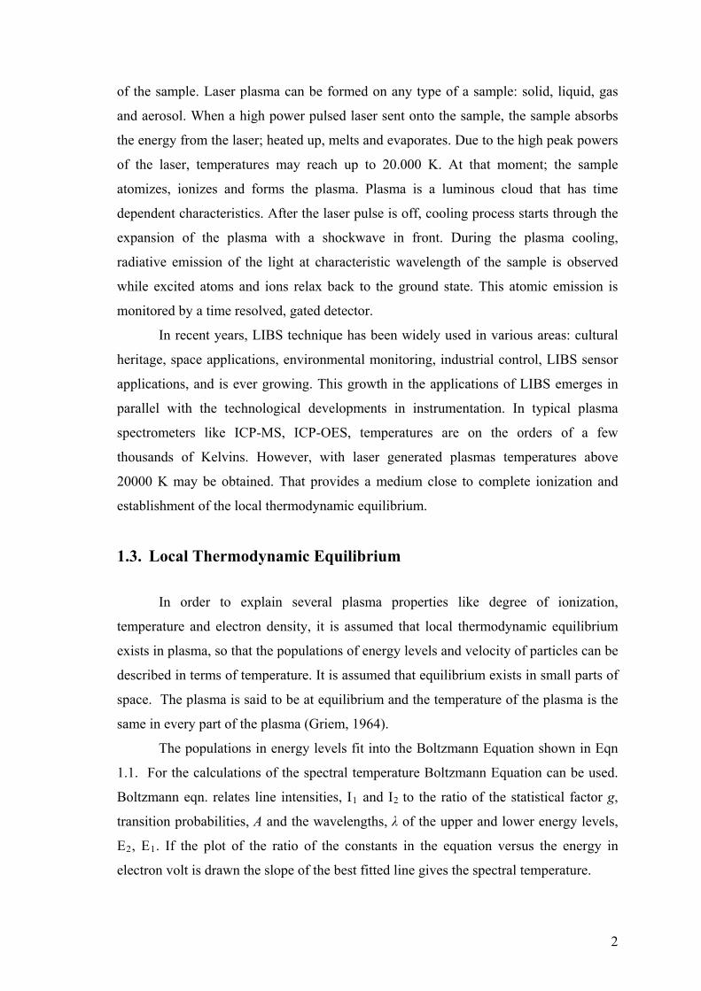
1.3. Local Thermodynamic Equilibrium
In order to explain several plasma properties like degree of ionization,
temperature and electron density, it is assumed that local thermodynamic equilibrium
exists in plasma, so that the populations of energy levels and velocity of particles can be
described in terms of temperature. It is assumed that equilibrium exists in small parts of
space. The plasma is said to be at equilibrium and the temperature of the plasma is the
same in every part of the plasma (Griem, 1964).
The populations in energy levels fit into the Boltzmann Equation shown in Eqn
1.1. For the calculations of the spectral temperature Boltzmann Equation can be used.
Boltzmann eqn. relates line intensities, I1 and I2 to the ratio of the statistical factor g,
transition probabilities, A and the wavelengths, λ of the upper and lower energy levels,
E2, E1. If the plot of the ratio of the constants in the equation versus the energy in
electron volt is drawn the slope of the best fitted line gives the spectral temperature.
2

kTEEAg
Ag
I
I/)(lnln 12
222
211
2
1
(1.1.)
The velocities of the species in plasma can be calculated by Maxwell Equation
(Eqn 1.2). In Maxwellian Equations m is the mass of an electron, v is the velocity, k is
the Boltzmann constant and T stands for the temperature.
kTm
ekT
mf 2/2
2/32
24)(
(1.2.)
In addition, the chemical composition of the plasma is explained by the Saha-
Bolztmann Equation given in Eqn 1.3.
kT
EEEET
Nh
mk
Ag
Ag
I
I
e
212/33
2/3
122
211
2
1 exp1)2(
2
(1.3.)
1.4. Advantages and Disadvantages of LIBS
There are advantages and disadvantages of this technique. First of all, LIBS
technique has little or no sample preparation. This is an advantage because it eliminates
possible contaminations and loss of analyte throughout the sample preparation steps.
Besides, LIBS may be easily applied to all forms of samples, solid, liquid and gas. Even
analyses of very hard samples are permitted. For solid samples depth profiling and
lateral resolution is possible. This advantage arises from the fact that LIBS systems use
only small amounts of sample. Craters with a few micrometers of diameters are
obtained with suitable optics. By the help of the use of fiber optic cables, LIBS system
can be applied as a remote analysis technique. Further more, the compact portable LIBS
set-ups enable field analysis. One of the major advantages of LIBS is its speed and
ability to make multi-elemental analysis. By using suitable spectrograph equipped with
a multi channel detector, analysis of dozens of elements in a single laser shot may take
just a second.
Contrary to the advantages of LIBS, there are some disadvantages. Since the
energy of laser may vary from one shot to another, the response monitored changes.
This 5-10% energy variation may lead to a problem during low level of quantification.
3

Therefore, in order to eliminate this disadvantage, several measurements may be
averaged. Also, during the analysis of solids, the surface composition may be different
than the bulk composition. Since the crater formed by the focused beam is just a few
micrometers in size and depth, the investigated area may not be a representative of the
whole sample. As a result of the above facts, the analytical figures of merit are not as
good as the other widely used atomic spectroscopic techniques such as ICP-OES and
AAS. The detection limits are in the range of hundreds of ppb, (µg/L), to ppm, (mg/L),
levels, but are improved by new studies. Table 1.1 shows some of the detection limits
from the literature.
1.5. Instrumentation
A LIBS set-up is typically composed of 3 main parts; laser, as the light source,
focusing optics, to focus the laser to form the plasma and to collect the emission, and
detection unit composed of a spectrometer and a detector.
The laser beam can be send on to the sample in two different directions
regarding the plasma image position on the slit. The plasma image can be parallel or
perpendicular to the slit height. By different orientations, the portion of the plasma
falling onto the slit changes, thus the response.
Figure 1.1. shows a typical LIBS set-up (Caceres et al., 2001). Here, the sample
is placed on a stage with a step motor. The beam from the laser sources are focused onto
the sample on this stage. After the plasma formation, the emission is collected by a fiber
optic cable which is connected to a monochromator and a detector. The triggering is
controlled by the computer.
4
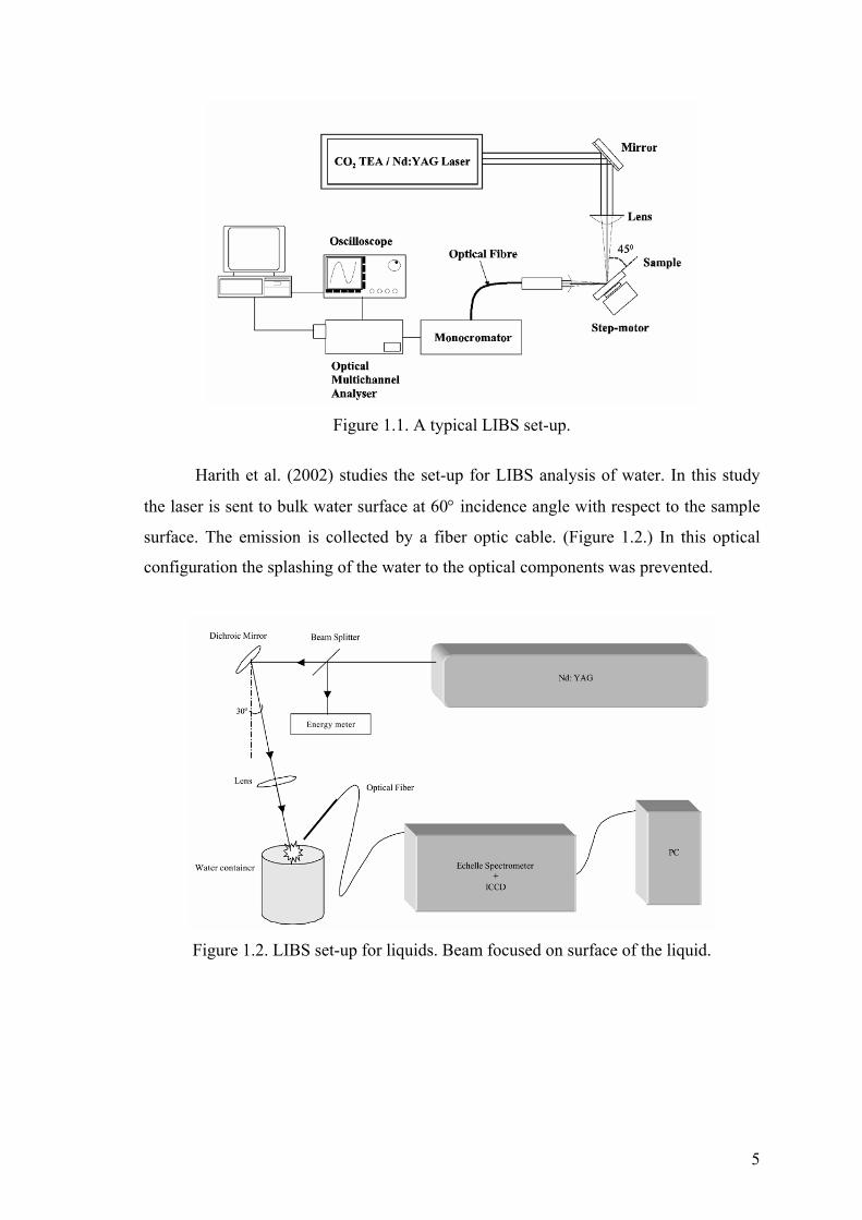
Figure 1.1. A typical LIBS set-up.
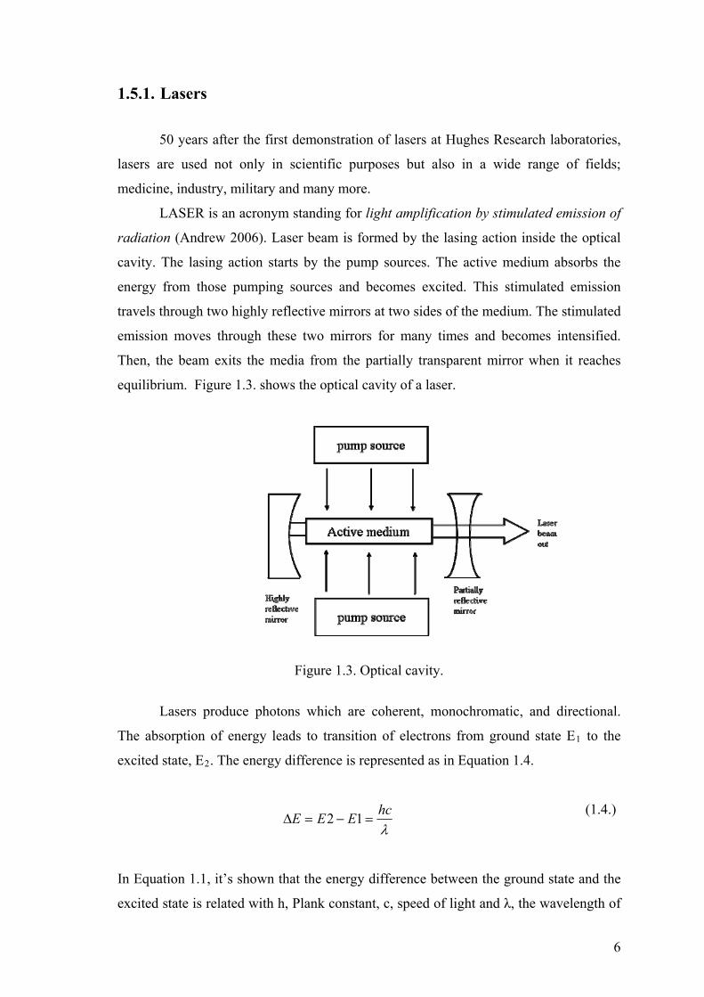
Harith et al. (2002) studies the set-up for LIBS analysis of water. In this study
the laser is sent to bulk water surface at 60 incidence angle with respect to the sample
surface. The emission is collected by a fiber optic cable. (Figure 1.2.) In this optical
configuration the splashing of the water to the optical components was prevented.
Figure 1.2. LIBS set-up for liquids. Beam focused on surface of the liquid.
5
1.5.1. Lasers
50 years after the first demonstration of lasers at Hughes Research laboratories,
lasers are used not only in scientific purposes but also in a wide range of fields;
medicine, industry, military and many more.
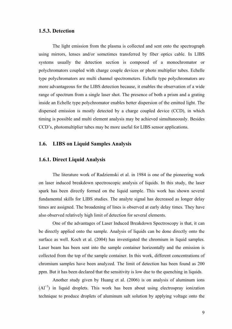
LASER is an acronym standing for light amplification by stimulated emission of
radiation (Andrew 2006). Laser beam is formed by the lasing action inside the optical
cavity. The lasing action starts by the pump sources. The active medium absorbs the
energy from those pumping sources and becomes excited. This stimulated emission
travels through two highly reflective mirrors at two sides of the medium. The stimulated
emission moves through these two mirrors for many times and becomes intensified.
Then, the beam exits the media from the partially transparent mirror when it reaches
equilibrium. Figure 1.3. shows the optical cavity of a laser.
Figure 1.3. Optical cavity.
Lasers produce photons which are coherent, monochromatic, and directional.
The absorption of energy leads to transition of electrons from ground state E1 to the
excited state, E2. The energy difference is represented as in Equation 1.4.
hc
EEE 12 (1.4.)
In Equation 1.1, it’s shown that the energy difference between the ground state and the
excited state is related with h, Plank constant, c, speed of light and λ, the wavelength of
6

the characteristic emission. Relaxation forms a radiation which is called stimulated
emission which represents the coherency, the same phase in space and time. Lasers are
the source of light amplification by the help of the stimulated emission.
Boltzmann distribution which represents the population of atoms in possible
energy levels is given in Equation 1.5.
KTEegg
NN /
2
1
1
2
(1.5.)
N2 stands for the population in the upper and lower energy levels. g is the
statistical weight of upper level, E is the upper state for emission and k is the Boltzmann
Constant (1.38 * 10-38 J/K). When N1 is more than N2, more energy levels are included;
the emission can take place in two or more levels.
There are different types of lasers varying on their active media or pump sources
and can be listed as solid state lasers, gas lasers, dye lasers and semiconductor diode
lasers. Only Nd:YAG laser as an example to solid state lasers will be presented under
the interest of this work. Some other examples of solid state laser other than Nd:YAG
laser are Cr:YAG and Nd:YLF. For the gas lasers, the active medium is composed of
gases and is pumped by electrical charges. He-Ne and CO2 lasers are some examples.
Dye lasers imply an active medium of dyes. Likewise, semiconductor materials such as
gallium arsenide and gallium nitrate are used in semiconductor lasers.
1.5.1.1. Nd:YAG Lasers
Neodymium-doped yttrium aluminum garnate, Nd:YAG, lasers are the most
commonly used and understood solid state lasers (Andrew 2006).
The pumping sources are the flash lamps whose energy is enough to excite the
atoms of the crystal. At each time the flash lamps are fired the active medium will emit
a light at a wavelength of fundamental emission, 1064 nm. On the other hand, by the
use of an optical device, harmonic generator, light emissions from near IR to UV region
at wavelengths of 532 nm, 356 nm, and 266 nm can be obtained as the second, third
and fourth harmonics, respectively.
7

When the absorption and emission energies are the same it is called a two level
laser system. Nd:YAG lasers which are four-level lasers are more efficient compared to
three or two level laser, because the excited state energies (E) are much higher than the
ground state, so does the population (N) in forth level.
Level 4
Level 3
hv=1064nm Level 2
Level 1
Figure 1.4. A four level laser scheme.
1.5.2. Optic Materials
All the optical materials used in LIBS set-ups should be specially designed for
the wavelength of the laser beam. The mirrors are used to direct the laser beam coming
out of the active medium. They are front surface coated and reflect the beam at 99.9 %
reflectivity. The focusing lenses focus the laser beam onto the sample spot to form the
plasma. In the same manner, the collecting lenses make the emission of the plasma
parallel and focus on the slit of the spectrograph. The diameter and the thickness of the
lenses are important to match the requirements of the detection system and eliminate
optical aberrations.
Besides to the lenses fiber optic cables are also used to manage the light because
they are easy to handle. They are mostly preferred in portable systems (Laserna et al.,
2008) and when the detection part of the system cannot get too close to the emission
part (Cremers and Radziemski, 2006).
8
1.5.3. Detection
The light emission from the plasma is collected and sent onto the spectrograph
using mirrors, lenses and/or sometimes transferred by fiber optics cable. In LIBS
systems usually the detection section is composed of a monochromator or
polychromators coupled with charge couple devices or photo multiplier tubes. Echelle
type polychromators are multi channel spectrometers. Echelle type polychromators are
more advantageous for the LIBS detection because, it enables the observation of a wide
range of spectrum from a single laser shot. The presence of both a prism and a grating
inside an Echelle type polychromator enables better dispersion of the emitted light. The
dispersed emission is mostly detected by a charge coupled device (CCD), in which
timing is possible and multi element analysis may be achieved simultaneously. Besides
CCD’s, photomultiplier tubes may be more useful for LIBS sensor applications.
1.6. LIBS on Liquid Samples Analysis
1.6.1. Direct Liquid Analysis
The literature work of Radziemski et al. in 1984 is one of the pioneering work
on laser induced breakdown spectroscopic analysis of liquids. In this study, the laser
spark has been directly formed on the liquid sample. This work has shown several
fundamental skills for LIBS studies. The analyte signal has decreased as longer delay
times are assigned. The broadening of lines is observed at early delay times. They have
also observed relatively high limit of detection for several elements.
One of the advantages of Laser Induced Breakdown Spectroscopy is that, it can
be directly applied onto the sample. Analysis of liquids can be done directly onto the
surface as well. Koch et al. (2004) has investigated the chromium in liquid samples.
Laser beam has been sent into the sample container horizontally and the emission is
collected from the top of the sample container. In this work, different concentrations of
chromium samples have been analyzed. The limit of detection has been found as 200
ppm. But it has been declared that the sensitivity is low due to the quenching in liquids.
Another study given by Huang et al. (2006) is on analysis of aluminum ions
(Al+3) in liquid droplets. This work has been about using electrospray ionization
technique to produce droplets of aluminum salt solution by applying voltage onto the
9

nozzle of the flow injection system. The aluminum salt solution has been
preconcentrated on ion-exchange column, before the nozzle. The laser beam has been
focused onto those droplets at the tip of the nozzle. This work has claimed that the
preconcentration has made an advantage on LIBS system.
Yaroshchyk et al. (2005) has given a comparison work of LIBS using liquid jets
and static liquids. This work shows most of the disadvantages of working with liquids
such as splashing and bubble formation on the surface of liquid samples. They have
shown that the liquid jets, in which the sample is thrown from a plastic funnel, is more
rapid and easy to acquire data than as in static liquid.
Caceres et al. (2001) has demonstrated a different methodology of LIBS for
quantitative analysis of trace metals in liquids. In this work, Al and Na ions were
determined in liquid samples that have been converted to ice by freezing in liquid
nitrogen. Low background levels have been obtained. The detection limits for Al and
Na has been declared as 1 ppm and 2 ppm respectively.
Gondal et al. (2007) has studied on determination of poisonous metals in paint
factories. Similar to the above work of Caceres, paint sample has been filtered and dried
at 105C. Then LIBS analysis has been carried out. They have shown that the results of
LIBS and ICP are similar to each other.
Janzen et al. (2005) has presented a novel HPLC-LIBS hyphenated technique. In
this method, first the sample is separated molecularly by HPLC and then by a
piezoelectric nozzle the separated specie is transferred to droplets. Later, each droplet is
analyzed by the laser focused onto the system. The data collection is accomplished by
Paschen Runge Spectrometer coupled with 31 PMTs to detect 31 different elements,
simultaneously. The voltage applied on the piezoelectric can be altered to form droplets
with different sizes. In this work the diameters of the droplets generated has been
declared as 50 to 100 m. Yet, in this study the authors has been faced with the
difficulties working with liquids. They have shown that the bulk liquid analysis has
some disadvantages such as very rapid decay of the plasma (approximately 1 s) and
bubble formation occur on the surface analysis of liquids by LIBS.
In general, LIBS analysis of liquids directly on the surface or in bulk suffers
from several obstacles, such as shockwave formation, bubble formation, splashing of
the sample and scattering of the laser beam. These difficulties have some negative
effects by reducing the data quality and hence the detection limit of the technique. In
10

order to eliminate these problems several approaches may be performed such as use of
multiple pulses, aerosol formation or chemical derivatization. (Unal et al., 2010)
1.6.2. Double Pulse LIBS
In order to obtain better emission signal intensities double laser pulses may be
used in analysis of liquids. Both of the lasers strike onto the sample, with a time
difference between the pulses. The first pulse usually heats and pre-ablates the sample.
On account of the enhanced ablation in double pulse LIBS the emission signals obtained
are in better spectral quality. Hahn et al. (2006) has demonstrated use of dual pulse in
analysis of aerosols and gases. The energy of the second pulse (290 mJ) they have used
was more energetic than the first one (100mJ/pulse) thus the plasma formed by the
second plasma were larger than the initial plasma. Their aerosol particles have been
carried by air to the sample cell. This study has given an example of the dual pulse
application on aerosols. The signal enhancements have been given as 4 fold.
Yoshiro et al. (1996) had experiments to determine the iron suspensions in water
by LIBS using two sequential lasers. The limit of detection has been highly improved
by the use of two sequential lasers. It has been found as 16 ppb for single pulse
excitation. By two sequential lasers, the particles in a liquid sample can be detected.
Furthermore, it has been declared that in limit of detection studies, other parameters
such as pulse energy, timing of two lasers are important.
1.6.3. LIBS on Aerosol Samples
Aerosol formation is an alternative method in liquids analysis by LIBS. Aerosols
can be generated by either a pneumatic nebulizer or an ultrasonic nebulizer.
One of the initiative works by Radziemski et al. in 1983 was the analysis of air
aerosols by LIBS. Beryllium, sodium, arsenic and mercury elements have been detected
in air. In this work the samples were introduced to the nebulizer/heater chamber. The
temperature has been above 100 C. Air concentrations have been calculated for
beryllium. The air concentration of beryllium, 0.6 ng/ g air corresponds to solution
concentration of 40 ng/mL. Also, in this work LIBS technique has been compared with
ICP and it has been declared that the detection limits of ICP results are much lower than
the LIBS concentrations.
11

Another work of Radziemski et al. (1988) gives another example for use of
pneumatic nebulizer in the analysis of cadmium, lead and zinc aerosols. They have
collected the aerosols on the filter and flame atomic absorption spectrometry method
has been used to see the mass of lead accumulated on filter. On the other hand, high
concentrations of samples have generated large particles and since the energy is fixed
the entire sample may not be fully atomized. They have also proved that the response of
lead analyte has been increased by addition of sodium element into the solution.
Moreover, the article by Cheng et al. (2000) has given an example of detection
of chromium by forming aerosols. Despite to the other studies, this time the aerosol
particles are generated by an atomizer. The diameter of the particles are measured and
found out to be 2.4 m ( 1.5 m). The detection limit for chromium in air has been
found as 4000 ng/m3. Besides, they have sought for the effect of laser wavelength and
found out that the lowest signal-to-noise ratio is calculated for 266 nm. They have
expressed the importance of laser energy for ionization of the analyte.
Panne et al. (2001) has also demonstrated an alternative way of analysis of
aerosols. In their work they stabilized the lead aerosols on filters in an automatic
system. Quartz fibers have been used as filtering medium. They have analyzed several
toxic elements such as Cd, Ni, As, Co, Mn, Sb, Cr, Tl, Sn, V, Cu and Pb. This method
can be taken as a model for detection of heavy metals in environment. They have
provided detection limits in air concentrations and amount of analyte per area of filter
paper. As the authors declare, deposition of particles on filters has brought advantage in
achieving better detection limits.
Also, Hahn et al. (2001) has developed an aerosol system for aerosol generation
and calibration by LIBS. They have used a pneumatic nebulizer and formed submicron
sized particles. They have placed a porous plate on top of the nebulizer and a co-flow of
the nitrogen is introduced to the system. Then the aerosols travel to the six-way sample
chamber. They have investigated the particle size of iron and titanium oxide particles by
TEM (Transmission Electron Microscopy). The range has been determined as 13.2 to
9.5 nm (7 nm).
In addition, Hahn et al. (2001) has shown on-line analysis of aerosol particles in
air. They have detected magnesium, aluminum, calcium and sodium on a holiday period
in town. They have used a commercially available air sampling system which produces
particles less than 10 m in diameter. The particles formed by this inlet are introduced
12
to a four-way sample cell. The cell is connected to a vacuum pump at one arm and at
another arm the laser is focused into the sample. Also by the help of a pierced mirror the
plasma emission is collected back to a spectrometer. They have also investigated the
particle sizes of the particles. They were in the range of 0.1 to 1.0 m. They have found
that since the fireworks are used more on holidays the particle distribution is found out
to be more. The mass concentrations in air are given as 46 ppt for aluminum, 0.65 ppb
for sodium and 0.21 ppb by mass for calcium on holidays.
Besides to all the above works, in literature there are some applications of
portable LIBS systems. One of them has been presented by Laserna et al. in 2003. Their
study was about a portable LIBS system for rapid on site analysis of steel. A probe
composed of laser with both focusing and collecting optics has been focused onto the
sample. The emission is transformed by fiber optic cable. In addition to the field
analysis, they have also demonstrated the same analysis in lab conditions with the same
probe design.
For the demonstration of particle-plasma interactions, Hohreiter and Hahn
(2006) show the non-homogeneity of the plasma of calcium particles. In this study the
aerosol particles are formed by a pneumatic nebulizer purged by HEPA filtered air. The
particle size distribution and shape of the aerosols have been determined using optical
microscopy. At different delay times plasma images are collected. At late times the
plasmas have been difficult to make qualitative analysis.
In another study by Hahn et al. (2007) pneumatic nebulization technique has
been used to generate particles of sodium and magnesium. The carrier gas used was air
filtered by HEPA filter. The particle sizes of the particles have been expected to be less
than 100 nm regarding to the TEM (Transmission Electron Microscopy) analysis. They
have also shown that addition of elements like copper, zinc or tungsten enhances the
analyte signal intensity. The additional elements cool down the plasma so that the
analyte signal gets higher. This piece of work is valuable in order to understand the
particle-plasma interactions.
In 2008, Laserna et al., this time, has worked on a stand-off design for the
detection of liquid aerosols. The LIBS plasma formed was at 10 meters distance. The
laser has been focused onto the particles on top of the nebulizer needle. High standard
deviation of the measurements leads to uncertainty yet the authors claim that the limit of
detection for sodium element is 55 ppm. The sizes of the particles generated are in size
range of 4 to 16 m for 1000 ppm sodium particles. They have also shown that the
13

14
aerosol concentration should not be so low, if so, the data does not represent the sample
and poor data is obtained. If the sampling rate is so high, then the laser beam cannot
penetrate through the aerosol particles.
Table 1.1. gives several examples from the literature and the declared detection
limits.
1.7. Aim of the Study
Many important elements which may be toxic or hazardous for the environment
need to be controlled in real time, on-line. Most frequently the instruments used for the
identification and determination of those elements are time-consuming, difficult to
conduct and require using high amount of sample or chemicals.
Regarding the advantages of the LIBS technique, such that the analysis provides
no sample preparation and the identity of the sample is not changed the sample can be
directly analyzed by LIBS. For that reason, a portable LIBS system can be designed,
constructed and optimized for the determination of the elements present in
environmental samples, both qualitatively and quantitatively.
Due to the obstacles faced on direct liquid LIBS analysis, this thesis focuses on
the conversion of the liquid sample into aerosols. In this work, an aerosol generation
system has been constructed and equipped with the commercially available parts. In the
second part of the work, qualitative and quantitative analysis have been shown. Also,
the detection limits will be discussed with the relevant studies from the literature.

Table 1.1. Detection limits from literature.
Element LOD Ref Method Notes: 0.0091 %w/v Onge et al Saline solutions Flowing and nonflowing surface analysis
1.6mg/L Aglio et al Double pulse – bulk liquid 8 mg/L Chadwick et al Liquid jet
33300 mg/m3 Molina et al Elements present in different ratio of gases
No quantification
1 mg/L Lin et al ESI Matrix effect. Same cation (K) different anions Solutions prepared with water&methanol (1:1)
173 mg/kg Gondal et al Calibration with powder form of the analyte//residues of liquid sample collected
Na
0.08 ug/ml Harith et al water 0.2 ug /g Gautier et al
Double Pulse/ Alloy
0.5ug/g Single Pulse / Alloy
Lasers oriented at different geometry
34 ug/L Lazic et al Bubble cavity 5 mg/L Aglio et al Double pulse – bulk liquid
0.4 mg/L Chadwick et al Liquid jet 0.21 mg/L Lazic et al Double pulse 200mg/kg Gondal et al Calibration with powder form of the analyte//residues of
liquid sample collected 1 ug/ml Harith et al Water- panaromic
Mg
3.19 mg/L Mohamed et al. Aluminum alloy 0.4 mg/L Chadwick et al Liquid jet Ca
301 mg/kg Gondal et al K 28 mg/kg Gondal et al
Calibration with powder form of the analyte//residues of liquid sample collected
15
15

CHAPTER 2
EXPERIMENTAL
2.1. LIBS Experimental Set-up
In this work a lab-made system has been designed, constructed and used for the
analysis of metal aerosols. The set-up may be divided into three sub categories. The first
step involves the generation of the aerosols; the second part is the heating/cooling and
drying unit for desolvation of the aerosols before entering into the sample cell. The last
part is the detection system in which spectral line intensities of the metal aerosols are
monitored.
2.1.1. Aerosol Generation
The pneumatic nebulizer used in our measurements throughout this study is
given in (Fig 2.1). After small amount of sample has been placed inside the nebulizer (7
mL), pressurized N2 gas has been applied from the bottom. The gas leaving the orifice
of the nebulizer converts the liquid sample into fine aerosol droplets. The liquid sample
has been divided into sub-droplet particles by the effect of the gas flowing at 3.5
mL/min. The uptake rate of the nebulizer is calculated to be 0.255mL/min at gas flow
rate of 3.5 mL/min. The nitrogen gas used from the nitrogen generator (NitroFlow) was
with 98.3% purity. The gas flow rate has been monitored by a flow meter (Cole
Parmer).
Figure 2.1. Medical used to convert aqueous solutions into aerosols.
16

2.1.2. Desolvation of the Aerosols
The solvent content of the aerosols should be removed to form clear, stable and
lowest possible plasma size and to eliminate instrumental and spectral interferences.
2.1.2.1. Heating/Cooling Unit
The aerosols formed by the pneumatic nebulizer have been traveling through a
glass tube fitting on top of the exit of the nebulizer. This glass tube is wrapped by
heating tape (Cole Parmer) and the temperature inside the glass heating tube has been
increased to 110 C. This temperature has been chosen in order to evaporate the solvent,
which is water. After the heating unit, the hot aerosols and the purge gas have been
moving into the mini condenser, which is connected to a cooler circulator (PolyScience)
adjusted to 4 C. Here, the evaporated solvent has been condensed and collected at the
end of the cooling unit. Much of the drain has been collected from this heating/drying
unit. This compact unit (Figure 2.2.) has been constructed at Ege University Glassware
Workshop. The efficiency of the heating/cooling unit has been determined using
Atomic Absorption Spectrometry (Therma Elemental Solaar AA Spectrometer). Drains
of 10 ppm Cu2+ solution have been collected. The results show that the analyte
concentration present in drain is 1 ppm. This shows that, 90% of the analyte is
transported to the sample cell while 10% is lost to the drain during the desolvation
process.
To sample cell
Gas outMembrane dryer
Gas in
Condenser
Drain
Gas
Pneumatic Nebulizer
Figure 2.2. The pictorial and schematic representation of the heating/cooling unit.
17

2.1.2.2. Membrane Drying
After the heating/cooling unit, the aerosols have been going through a naphion
membrane dryer (Perma Pure PD50). The naphion structure is selective to water.
(What’s Naphion?® Perma Pure LLC). Here, the aerosols have been dried by a
countercurrent flow of drying gas (nitrogen) with respect to sample flow. The excess
moisture has been given out of the membrane dryer. In order to test the removal of the
moisture content of the aerosols in the membrane unit, silica gel beads have been placed
at the exit of the membrane drying gas. The color change of the silica gel beads from
blue to pink was indicating the removal of water content of the aerosols. At last, the dry
aerosols enter the sample cell.
2.2. Instrumental
All of the materials used are specially manufactured for LIBS systems. A Q-
switched Nd:YAG laser (Quanta-Ray Lab-170, Spectra Physics) has been used as the
laser source working at second harmonics, 532 nm. The laser pulses have 10 ns duration
at 10 Hz repetition rate. The laser beam has been reflected by the highly reflective
mirrors (coated, 532 nm reflective, New Focus,) towards the sample cell. The lens used
to focus the laser beam has 5 cm focal length and 1 inch outer diameter (Thorlabs). The
collimating lenses used to collect the plasma image onto the spectrograph were in 5 cm
and 17.5 cm focal length (Thorlabs). The energy of the incoming laser beam has been
measured by a power meter head (Nova II, Ophir, Israel). The teflon sample cell, with
five arms, each 1 inch outer diameter, has been designed in our group previously (Unal
et al 2009) and manufactured in a local machine shop in Urla, İzmir. The arms at which
the laser beam entering the cell and the emission to be collected are covered with quartz
windows. The medium inside the sample cell have been kept uniformly flowing using a
vacuum pump (Edwards) connected to a third arm of the sample cell. The plasma image
has been focused onto an Echelle type spectrograph (Mechelle 5000 Andor Inc.)
coupled with an ICCD detector (iStar DH734, Andor Inc.). The delay time (td) is the
time that the detector gets on and starts data acquisition. The gate width (tg) determines
the amount of time that the detector collects light. The delay time (td) and gate width
(tg) have been optimized for each of the elements separately. All the system
specifications have been summarized in Table 2.1.
18

Two different experimental LIBS set-up configurations have been constructed in
this work which are horizontal and telescopic beam set-up. Horizontal beam set-up is
the configuration in which the laser beam travels horizontally with respect to the optic
table, entering the sample cell from the side arms. The telescopic beam set-up is the
configuration in which the laser beam enters to the sample cell from the top,
perpendicular to the optical table. The horizontal (a) and telescopic (b) beam set-up
designs are shown schematically in Figure 2.3.
The size measurements of the aerosol particles have been accomplished by
Malvern MasterSizer HD-2000 present at İYTE Chemistry Department. The aerosols
have been introduced to the instrument exactly the same way as in aerosol generation
system discussed above.
19

(a)
Sample introduction unit
slit
(b)
(c)
Figure 2.3. Horizontal (a) and telescopic (b) beam setup, (M: mirror). (c) Pictorial representation of the telescopic beam set-up.
M1
Echelle Spectrograph + ICCD
Nd-Y
AG
532 nm
M2
M3 M4 Sample introduction
unit
Laser beam direction
Plasma expands in a direction towards incoming laser beam
Plasma moves along the slit height
slit
Nd-Y
AG
532 nm
Collimating Lenses
Plasma moves along the slit width Echelle Spectrograph + ICCD Laser beam
direction Plasma expands in a direction towards incoming laser beam Focusing
Lens
Mirror
20

Table 2.1. LIBS system specifications. Q-switched Nd: YAG laser Power meter 532 nm reflective mirrors Focusing lens Collimating lenses Echelle spectrograph ICCD detector Pneumatic nebulizer Heating-cooling unit Heating tape Cooler Sample Cell Vacuum Pump Membrane Dryer Quartz Windows Nitrogen Genetaror Flow Meters
Quanta-Ray Lab-170, Spectra Physics (California-USA) PE50BB-DIF-V2, Nova II, Ophir (Israel) 1″ OD, coated, 532 nm reflective (New Focus, Darmstad-Germany) 5 cm (1″ OD, Thorlabs) 5 cm (1″ OD, Thorlabs ) 17.5 cm (1″ OD, Thorlabs) Mechelle 5000, Andor, f/7 (European) iStar DH734, Andor Inc. (European) Medical Nebulizer Handmade glassware Cole Parmer, cloth insulated PolyScience Standard Digital Model 9106 5-way handmade Teflon Edwards PermaPure PD-50 Naphion 1″ OD quartz NitroFlow Lab Cole Parmer
21
2.2.2. Detection System
Through out the experiments an Echelle type spectrograph coupled with an
ICCD type detector has been (resolution λ=0.4 nm) used. An echelle type spectrograph
provides good resolution (wavelength coverage between 200-900 nm) with an added
benefit of multi-element capability. The resolved wavelengths have been detected by 2-
D array ICCD camera. With an ICCD camera rapid data acquisition with nanosecond
time windows can be achieved. Time resolved measurements allow plasma emission to
be monitored at different times of the plasma decaying. Suitable delay times and gate
widths have been found from the systematical investigation of the decaying laser
plasma at the specific analyte peaks. Usually after 4 s of delay times the ICCD orders
have been eliminated.
2.3. Reagents
Throughout the experiments fresh solutions have been prepared from the
analytical grade solid salts of the metals; such as sodium chloride (Riedel), anhydrous
calcium chloride (Fluka), magnesium chloride (Riedel) and potassium chloride
(CarloErba) using ultra pure water (18).
The nitrogen gas used to purge through the pneumatic nebulizer and naphion
membrane dryer has been obtained from NirtoLab nitrogen generator at 98% purity.
For the multi element analysis a real sample of mineral water (KULA) has been
used. Before the analysis, the mineral water has been kept in ultrasonic water bath for 5
minutes for degassing. Then the sample is directly introduced into the system. Also, tap
water from the laboratory has been used for the multi-element analysis as well.
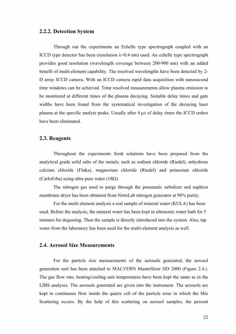
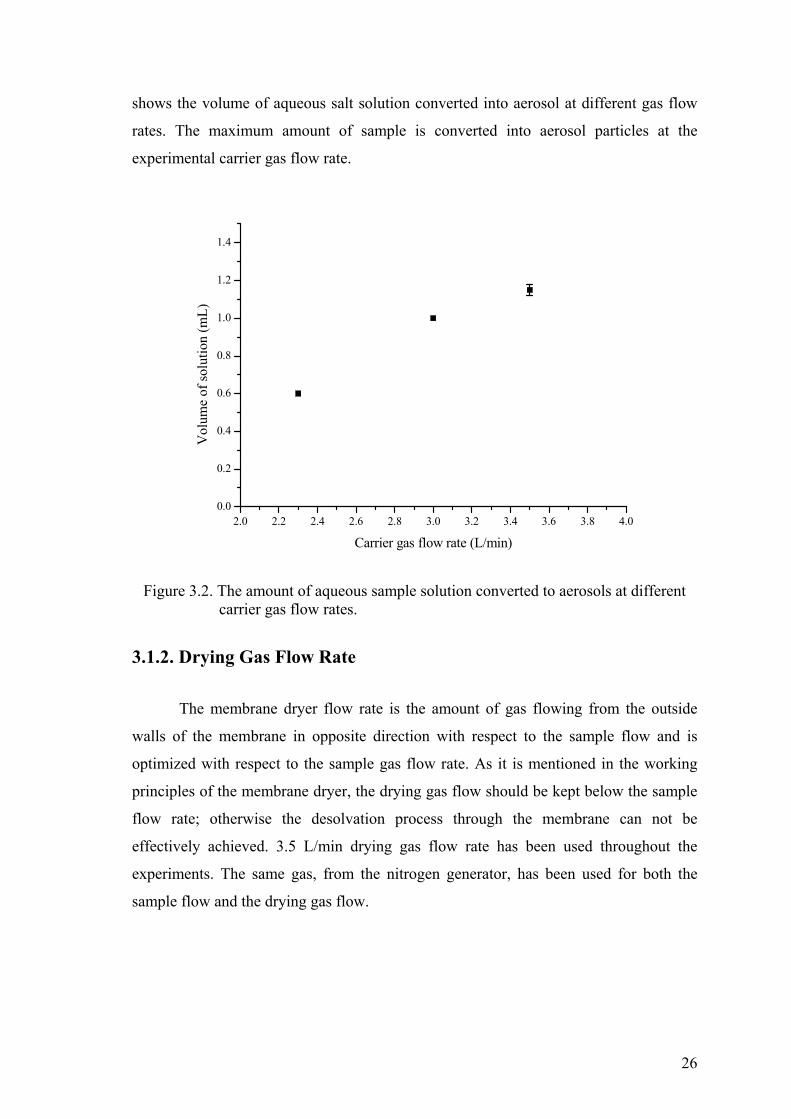
2.4. Aerosol Size Measurements
For the particle size measurements of the aerosols generated, the aerosol
generation unit has been attached to MALVERN MasterSizer HD 2000 (Figure 2.4.).
The gas flow rate, heating/cooling unit temperatures have been kept the same as in the
LIBS analyses. The aerosols generated are given into the instrument. The aerosols are
kept in continuous flow inside the quartz cell of the particle sizer in which the Mie
Scattering occurs. By the help of this scattering on aerosol samples, the percent
22
distributions are obtained. In the second part of the size measurements, the membrane
dryer has been attached at the exit of the aerosol generation unit. The effect of
membrane dryer on particle size has been studied.
Figure 2.4. The aerosol generation unit attached to the particle sizer.
23

CHAPTER 3
RESULTS AND DISCUSSION
In this work, a LIBS system has been designed and constructed from its
commercially available parts to monitor the LIBS signal of nebulized salt aerosols;
NaCl, CaCl2, MgCl2 and KCl. The construction of the LIBS system and functions of
each component has been discussed in detail, in Chapter 2.
There are some experimental and instrumental parameters to be optimized
before obtaining representative LIBS spectra. The experimental parameters may be
listed as the nebulizer flow rate and membrane dryer gas rate. The instrumental
parameters are laser energy, delay time, gate width and gain.
3.1. Experimental Parameters
The experimental parameters refer to the variables that may be optimized
regarding the aerosol generation part of the experimental set-up. These are the flow
rates of sample and membrane dryer gas.
3.1.1. Effect of Sample Flow Rate on Signal Intensity
The sample flow rate is the actual gas flow rate applied from the bottom of the
nebulizer to generate and transfer aerosol particles from the nebulizer to sample/plasma
cell. During our measurements sample gas flow rate has been optimized. For this
purpose LIBS signal measurements have been performed at different gas flow rates
between 2.3 and 3.5 L/min.
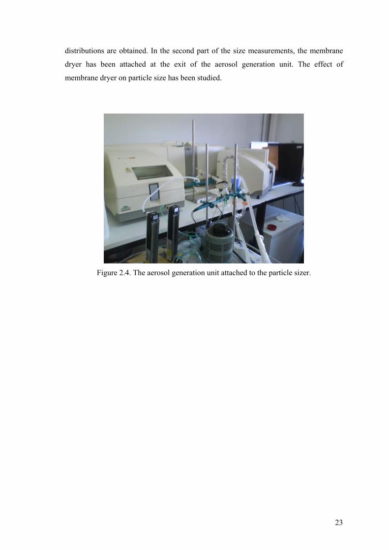
As it can be seen in Figure 3.1, the signal intensities of the resonant sodium lines
588.9 and 589.6 nm increase as the flow rate increases, due to increased amount of
aerosols carried into the sample cell. For this study, the optimum flow rate has been
found as 3.5 L/min. 2.3 L/min is the minimum flow rate required to observe LIBS
signal. Below this value there has been no sample transferred to the sample cell. Flow
rates higher than 3.5 L/min. resulted with the removal of the gas tubing from the
24
nebulizer due to an increased amount of gas pressure. Therefore, the highest sample gas
flow rate has been selected as 3.5 L/min. In addition, flow rate higher than 3.5 L/min
has resulted with the generation of a high amount of aerosol particles and the plasma
induced inside the sample cell has been highly moving. This movement was leading
plasma image to be larger and to move more on the slit of the spectrograph. This
situation might cause spectral and analytical disadvantages. The movement of the
plasma image on slit may lead to distortions of the image. Besides the plasma image
part which is left outside the slit, may reduce the analyte signal. For the later reasons,
the experiments have been done successively, on the same day, using vertical beam set-
up. In addition, a vacuum pump has been connected to one of the arms of the sample
cell, to prevent overloading of aerosol particles inside the sample cell. A constant flow
of aerosols have been accomplished inside the sample cell by the suction, and the
pressure inside has been checked by a gauge control. The pressure inside the sample cell
has been kept at atmospheric pressure.
0
2000
4000
6000
8000
1.5 2 2.5 3 3.5 4 4.5
gas flow rate (L/min)
Rel
ativ
e In
tens
ity (
AU
588.9 nm
589.6 nm
Figure 3.1. Effect of gas flow rate on Na signal intensity (50 ppm Na, 60mJ laser pulse energy, td=5s and tg=1ms have been used with 10 shot accumulation).
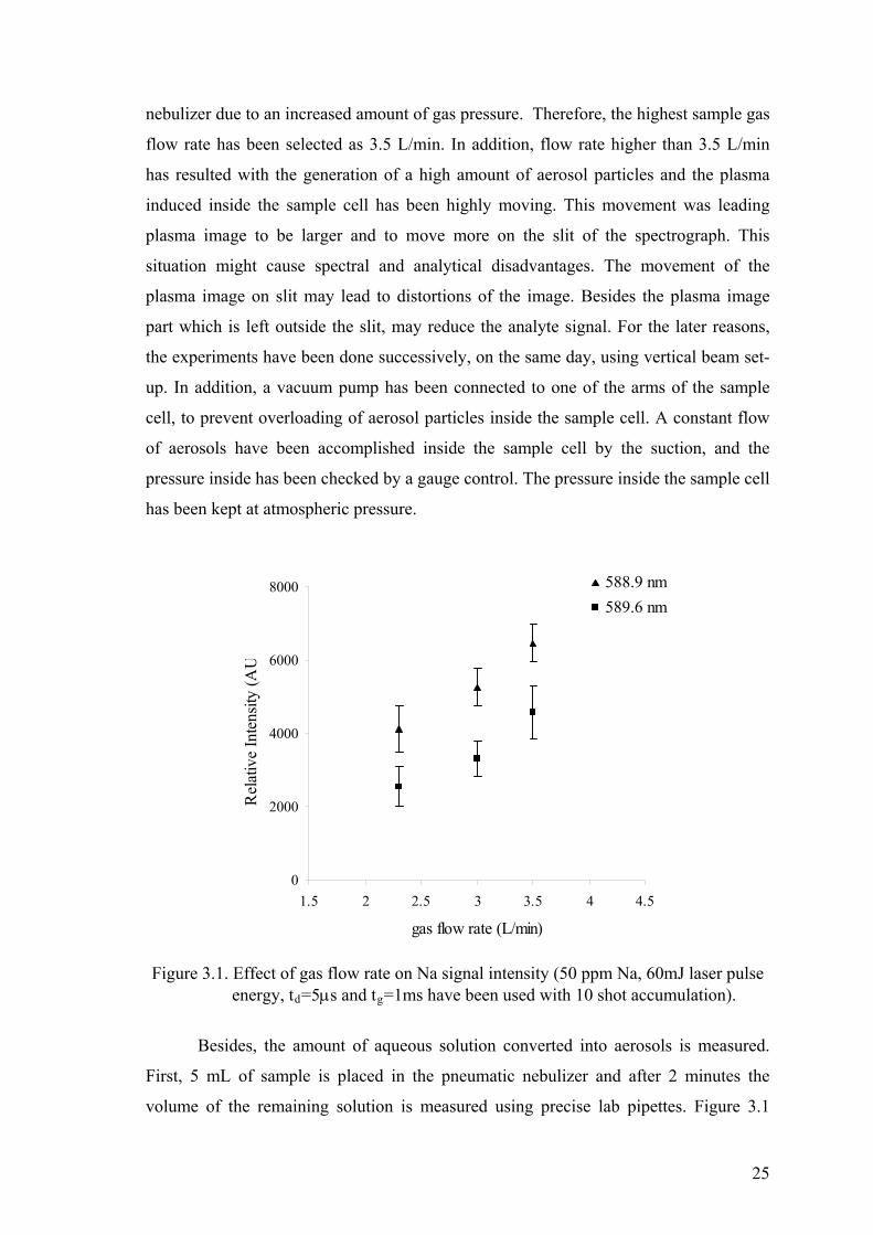
Besides, the amount of aqueous solution converted into aerosols is measured.
First, 5 mL of sample is placed in the pneumatic nebulizer and after 2 minutes the
volume of the remaining solution is measured using precise lab pipettes. Figure 3.1
25
shows the volume of aqueous salt solution converted into aerosol at different gas flow
rates. The maximum amount of sample is converted into aerosol particles at the
experimental carrier gas flow rate.
2.0 2.2 2.4 2.6 2.8 3.0 3.2 3.4 3.6 3.8 4.00.0
0.2
0.4
0.6
0.8
1.0
1.2
1.4
Vol
ume
of s
olut
ion
(mL
)
Carrier gas flow rate (L/min)
Figure 3.2. The amount of aqueous sample solution converted to aerosols at different carrier gas flow rates.
3.1.2. Drying Gas Flow Rate
The membrane dryer flow rate is the amount of gas flowing from the outside
walls of the membrane in opposite direction with respect to the sample flow and is
optimized with respect to the sample gas flow rate. As it is mentioned in the working
principles of the membrane dryer, the drying gas flow should be kept below the sample
flow rate; otherwise the desolvation process through the membrane can not be
effectively achieved. 3.5 L/min drying gas flow rate has been used throughout the
experiments. The same gas, from the nitrogen generator, has been used for both the
sample flow and the drying gas flow.
26
3.2. Instrumental Parameters
Instrumental parameters are the variables that are related to the spectroscopy part
of the system. They are listed as laser energy, delay time, gate width, and gain.
3.2.1. Effect of Laser Pulse Energy on Signal Intensity
Laser pulse energy is an important parameter in laser produced plasmas. The
size, temperature and hence the extent of ionization is very much dependent on the laser
pulse energy. This laser pulse energy is the source of energy for evaporation,
atomization and ionization of the aerosol particles when it is focused inside the sample
cell.
The variation in LIBS signal intensity as the energy of the incoming beam
increases is shown in Figure 3.3. In Figure 3.3(a) laser pulse energy has been optimized
with respect to peak heights of the Na(I) lines, 588.9 and 589.6 nm, whereas in Figure
3.3(b) 279.5 nm line of magnesium was investigated. In general, signal intensity
increases as the pulse energy increases for both elements, however, a drastic increase in
signal intensity after 50 mJ/pulse laser energy has been observed for Na. At laser pulse
energies higher than 70 mJ/pulse, Na line intensity does not increase linearly that might
be associated with the self absorption effect that is generally observed in laser plasmas.
Therefore, 60 mJ/ pulse laser energy was chosen as optimum laser energy for the rest of
the measurements for sodium. Similar results have been observed for Mg line as in
sodium element case.
27

0
1000
2000
3000
4000
5000
0 20 40 60 80 100 120
energy(mJ/pulse)
Rel
ativ
e In
ten
sity
(A
.U)
589 nm Na(I)
589.6 nm Na (I)
(a)
(b)
750
950
1150
1350
1550
1750
1950
2150
30 40 50 60 70 80 90 100
energy (mJ/pulse)
Rel
ativ
e In
ten
sity
(A
U)
Figure 3.3. LIBS signal intensity variation of (a) 588.9 nm and 589.6nm Na(I), (b) 280.2 nm Mg(I) and (c) 766.6 nm K(I) lines with respect to laser
energy (continued on next page).
28
(c)
100
150
200
250
300
350
400
450
500
60 80 100 120 140 160
energy (mJ/pulse)
Pea
k A
rea
(AU
)
766.6 nm K(I)
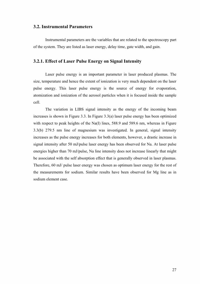
Figure 3.3. (cont) LIBS signal intensity variation of (c) K(I) 766.6 nm line with respect to laser energy.
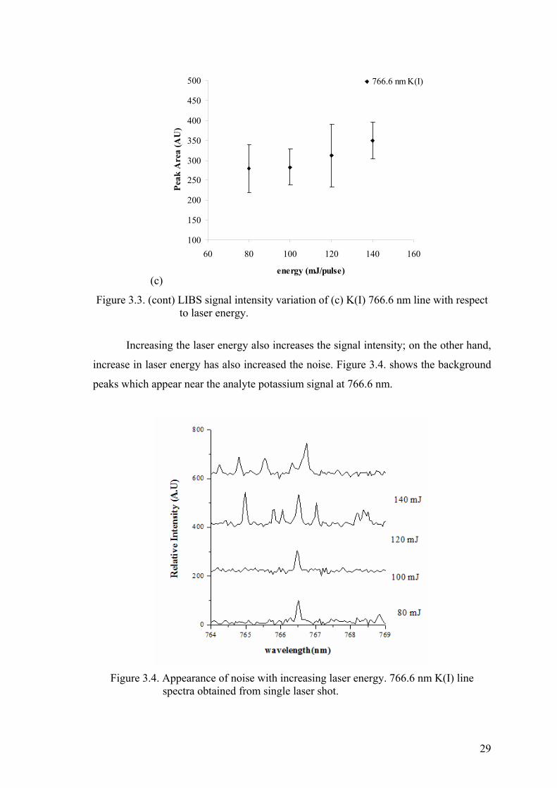
Increasing the laser energy also increases the signal intensity; on the other hand,
increase in laser energy has also increased the noise. Figure 3.4. shows the background
peaks which appear near the analyte potassium signal at 766.6 nm.
Figure 3.4. Appearance of noise with increasing laser energy. 766.6 nm K(I) line spectra obtained from single laser shot.
29
3.2.2. Time Resolution
Time resolution has great importance for the acquisition of the data at the correct
instant. Delay time (td) and gate width (tg) are the two timing options that need to be
optimized.
Usually, in order to get rid of the structured and highly noisy spectra due to the
continuous background emission at early times, late delay times on the orders of 4-5 s
have been preferred. Gate widths from hundreds of microseconds to several
milliseconds are possible depending on the lifetime of the species under investigation.
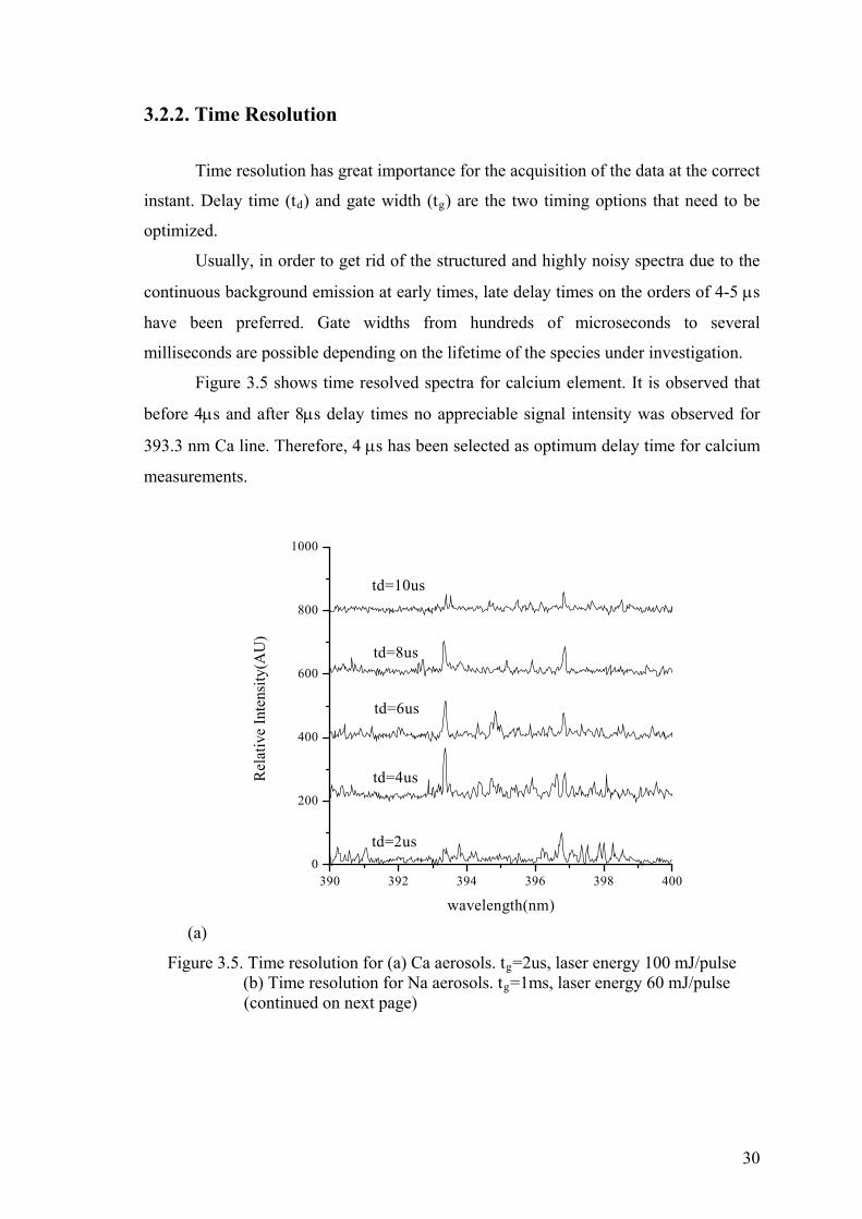
Figure 3.5 shows time resolved spectra for calcium element. It is observed that
before 4s and after 8s delay times no appreciable signal intensity was observed for
393.3 nm Ca line. Therefore, 4 s has been selected as optimum delay time for calcium
measurements.
(a)
390 392 394 396 398 4000
200
400
600
800
1000
Rel
ativ
e In
tens
ity(
AU
)
wavelength(nm)
td=2us
td=4us
td=6us
td=8us
td=10us
Figure 3.5. Time resolution for (a) Ca aerosols. tg=2us, laser energy 100 mJ/pulse (b) Time resolution for Na aerosols. tg=1ms, laser energy 60 mJ/pulse
(continued on next page)
30

(b)
586 587 588 589 590 591 592 593 594 595
0
1000
2000
3000
4000
5000
6000
7000
Td=2us
Td=5us
Td=10us
Wavelength (nm)
Rel
ativ
e In
tens
ity
(AU
)
Figure 3.5. (cont) Time resolution for Na aerosols. tg=1ms, laser energy 60 mJ/pulse
Gathering spectral information at the early times of the spectra may lead to
spectral order lines to appear. These giant orders due to the presence of high
background depress the presence and appearance of the analyte peak. Figure 3.6 shows
the spectral quality of the early plasma, when 10 mg/L sodium solution is aspirated into
the system, gate width at 2ms.
31

200 400 600 8000
2000
4000
6000
8000
10000
12000
Rel
ativ
e In
tens
ity
(AU
)
wavelength (nm)
td=2us
td=1us
td= 500ns
Figure 3.6. Spectra of early plasma. Laser energy 60mJ, gate width 2 ms.
3.2.3. Detector Gain
Another instrumental parameter to be considered is the gain applied on the
detector. Gain is the numerical quantity related with the potential applied across the
multichannel plate and affects the number of counts of photoelectron (Andor
Technology, 2003).
The effect of gain applied to the detector has shown its importance to reveal the
analyte peak from the high background. Figure 3.7 shows the effect of gain on 10 ppm
K+ solution aspired into the system. As it can be seen from the figure, a barely
observable K signal at 766.6 nm with 100 gain becomes easily observable with a drastic
enhancement at the gain of 200.
32

Figure 3.7. Effect of gain on potassium aerosols. td=4s, tg= 5s, laser energy 140 mJ.
3.3. Qualitative Analysis
The LIBS spectra include qualitative and quantitative information about the
sample being analyzed. The characteristic peaks are observed as a function of
spectrometer resolution for qualitative analysis.
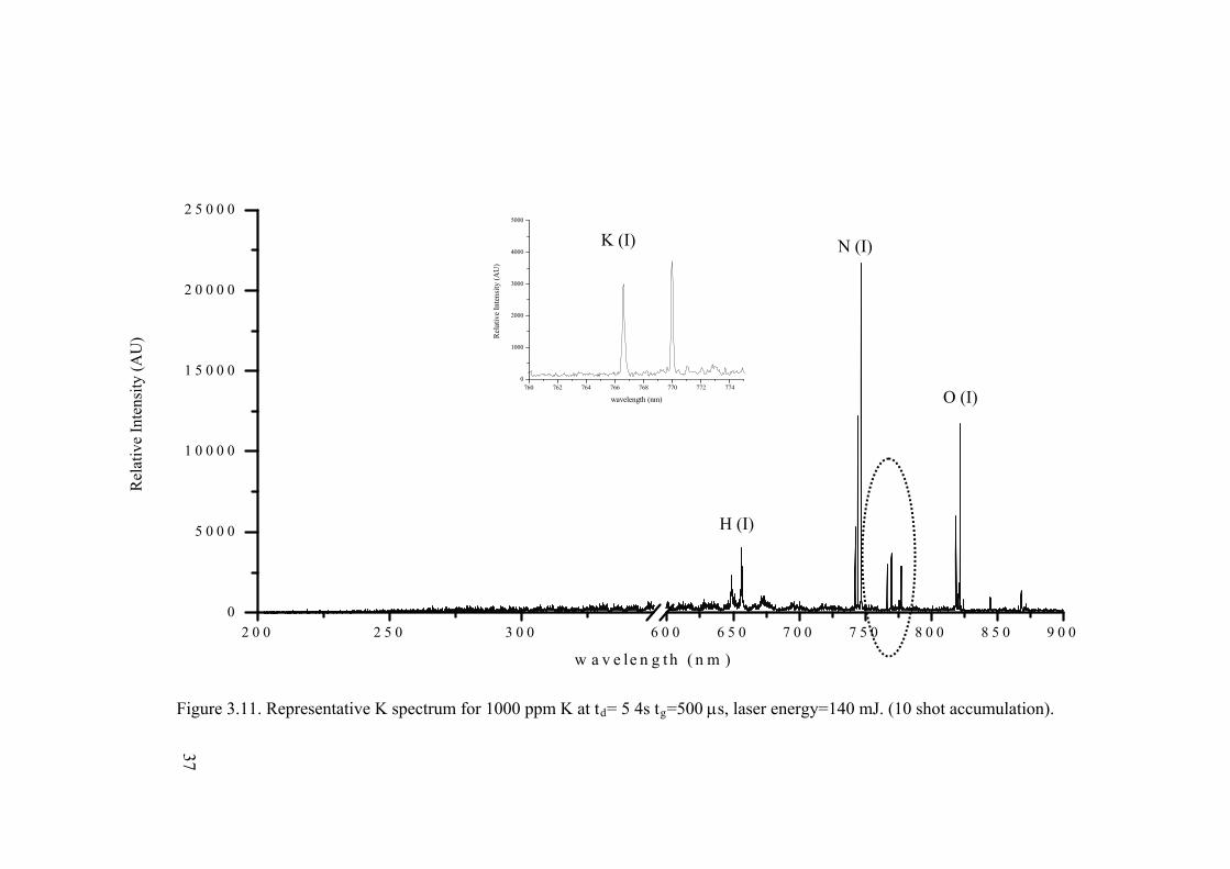
3.3.1. Representative Spectra
The representative LIBS spectra for sodium, calcium, magnesium and potassium
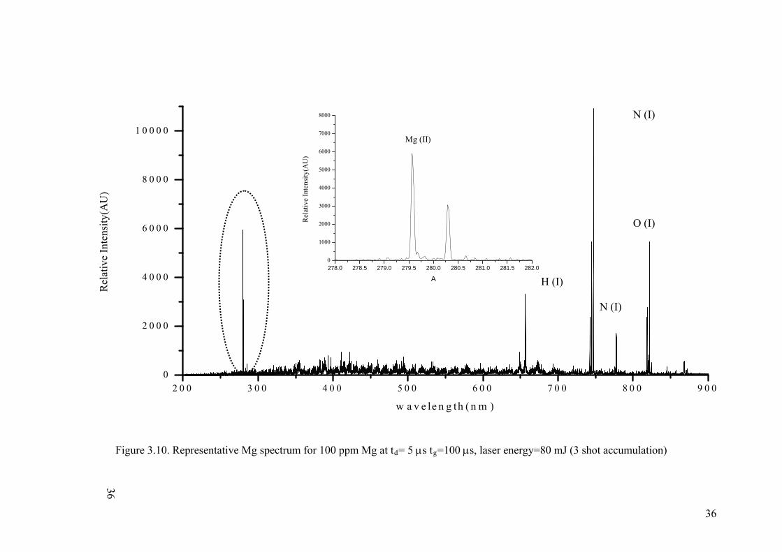
emissions have been depicted Figure 3.8., 3.9., 3.10. and 3.11. respectively. The most
probable resonance transitions of each element at 588.9 nm and 589.6 nm for sodium,
393.3 nm and 396.8 nm Ca, 279.5 nm for Mg have been observed with baseline
separation. In each spectra, hydrogen line at 656.3 nm coming from the moisture
content of the metal aerosols was clearly observed.
33

34
2 0 0 3 0 0 5 0 0 7 0 0 8 0 0 9 0 00
5 0 0 0
1 0 0 0 0
1 5 0 0 0
2 0 0 0 0
6 0 0
Rel
ativ
e In
tens
ity
(AU
)
w a v e l e n g t h ( n m )
586 587 588 589 590 591 592 593 5940
2000
4000
6000
8000
10000
Figure 3.8. Representative Na spectra for 100 ppm Na at td= 5 us tg=1 ms, laser energy=60 mJ (10 shot accumulation)
.
Rel
ativ
e In
etns
ity
(AU
)
wavelength(nm)
H (I)
N (I)
O (I)
N (I)
Na (I)
34

35
2 0 0 4 0 0 6 0 0 8 0 0
0
1 0 0 0 0
2 0 0 0 0
3 0 0 0 0
4 0 0 0 0
5 0 0 0 0
6 0 0 0 0
7 0 0 0 0
Rel
ativ
e In
tens
ity(A
U)
w avelen g th (n m )
Figure 3.9. Representative Ca spectrum for 100 ppm Ca at td= 5us tg=10us, laser energy=80 mJ (10 shot accumulation)
390 392 394 396 398 4000
10000
20000
30000
40000
50000
60000
70000
80000
Rel
ativ
e In
tens
ity
(AU
)
wavelength (nm)
N (I)
Ca (II)
35
2 0 0 3 0 0 4 0 0 5 0 0 6 0 0 7 0 0 8 0 0 9 0 0
0
2 0 0 0
4 0 0 0
6 0 0 0
8 0 0 0
1 0 0 0 0
N (I) R
elat
ive
Inte
nsity
(AU
)
w a v e le n g th ( n m )
278.0 278.5 279.0 279.5 280.0 280.5 281.0 281.5 282.00
1000
2000
3000
4000
5000
6000
7000
8000
Mg (II)
Rel
ativ
e In
tens
ity(
AU
)
A
O (I)
H (I)
N (I)
Figure 3.10. Representative Mg spectrum for 100 ppm Mg at td= 5 s tg=100 s, laser energy=80 mJ (3 shot accumulation)
36
36
37
2 0 0 2 5 0 3 0 0 6 0 0 6 5 0 7 0 0 7 0 0 8 5 0 9 0 0
0
5 0 0 0
1 0 0 0 0
1 5 0 0 0
2 0 0 0 0
2 5 0 0 0
5 0 8
Figure 3.11. Representative K spectrum for 1000 ppm K at td= 5 4s tg=500 s, laser energy=140 mJ. (10 shot accumulation).
O (I)
Rel
ativ
e In
tens
ity (
AU
)
w a v e le n g th ( n m )
760 762 764 766 768 770 772 7740
1000
2000
3000
4000
5000
H (I)
N (I) K (I)
Rel
ativ
e In
tens
ity
(AU
)
wavelength (nm)
37

3.3.2. Effect of Membrane Dryer on H- Line
The membrane dryer made up of naphion is selective to moisture content of the
sample flowing through. The sample has been dried by a countercurrent flow of a
membrane drying gas, and has been given out of the naphion membrane. The humidity
of the gas coming out of the membrane dryer has been checked by placement of blue
silica gels on the exit of the drying gas. The blue color of the silica gel (containing
Cobalt salt) (Tekkim Blue Silica Gel) has changed to pink, in few minutes of analysis.
As Figure 3.13 indicates the use of membrane dryer has also decreased the
background and especially the dominant H line (656.3 nm) has become lower in
intensity. This was advantageous to reveal the analyte signal as shown in Figure 3.12.
The intensity of the Na(I) 588.9 and 589.6 nm lines have increased when the membrane
dryer is attached to the aerosol generation unit.
586.0 586.5 587.0 587.5 588.0 588.5 589.0 589.5 590.0 590.5 591.0 591.5 592.00
500
1000
1500
2000
2500
3000
3500
4000
4500
5000
Rel
ativ
e In
tens
ity
(AU
)
wavelength (nm)
with membrane dryer without membrane dryer
Figure 3.12. The decrease in intensity of 588.6 and 589.6 nm Na(I) line when membrane dryer is used.
38

650 652 654 656 658 660 6620
2000
4000
6000
8000
10000
Rel
ativ
e In
tens
ity
(AU
)
wavelength (nm)
with membrane dryer without membrane dryer
Figure 3.13. The decrease in intensity of 658.3 nm H line when membrane dryer is used.
3.3.4. Effect of Dessicant Prior to Membrane Dryer
A small glass adaptor has been placed between the exit of the heating/cooling
unit and entrance of the membrane dryer. Inside, blue silica gels have been tucked in. At
the end of several respective measurements, the color of the blue silica gel has turned to
pink. This has been tried with 750 ppb Ca2+ solution. It has been observed that the peak
areas of ionic calcium lines (393.3, 396.8 nm) and oxygen line (777 nm) have increased
slightly. On the other hand this adaptation has been avoided because after a while the
accumulation of analyte on silica may occur. Thus, it is not favored and not used in any
other experiments. Table 3.1 shows the slight increase in average peak areas of 10
consecutive measurements.
Table 3.2. The icrease in peak area for Ca(II) 393.3 nm line when a dessicant is placed at the exit of the heating/ cooling unit.
Relative Intensity (AU) Ca(II) 393.3 nm O(I) 777 nm
Without dessicant 185 (19.3) 128 (42.7)
With dessicant 292 (45.8) 297 (46.9)
39

3.4. Quantitative Analysis
In order to show the applicability of the developed system for the quantitative
analysis of the aqueous metal salts, the strongest emission lines of the analyte have been
chosen to be monitored. These spectral lines listed in Table 3.2. are used to construct
calibration graphs of each element studied.
Table 3.4. Spectral emission lines of the elements studied.
Element Wavelength (nm)
Na(I) 588.9, 589.6
Ca (II) 393.6, 396.8
Mg (I)
Mg(II)
279
279.5, 280.2
K(I) 766.5
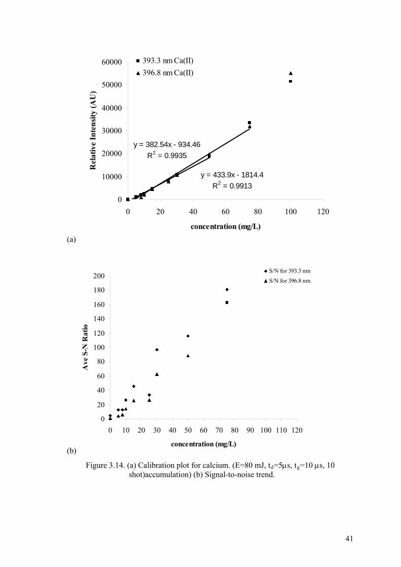
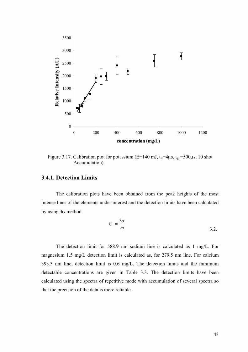
The calibration graphs have been drawn by using solutions from 5 mg/L to 100
mg/L analyte concentration and each point in the graphs represents a signal intensity
obtained by averaging 11 consecutive laser pulses. Figure 3.14, 3.15 and 3.16 and 3.17
shows the calibration plots constructed for Ca, Na, Mg and K respectively. In the
calibration graphs it can be seen that after 40-50 mg/L analyte concentration the
deviation from the linearity occurs. This non-linearity can be explained by the plasma
shielding effect (Cremers and Radziemski, 2006) in which the presence of excessive
amounts of particles inside the plasma leads to the formation of a thick plasma in which
the laser beam cannot penetrate into the particles in the focal volume.
40
(a)
y = 382.54x - 934.46
R2 = 0.9935
y = 433.9x - 1814.4
R2 = 0.9913
0
10000
20000
30000
40000
50000
60000
0 20 40 60 80 100 120
concentration (mg/L)
Rel
ativ
e In
ten
sity
(A
U)
393.3 nm Ca(II)
396.8 nm Ca(II)
(b)
0
20
40
60
80
100
120
140
160
180
200
0 10 20 30 40 50 60 70 80 90 100 110 120
concentration (mg/L)
Ave
S-N
Rat
io
S/N for 393.3 nm
S/N for 396.8 nm
Figure 3.14. (a) Calibration plot for calcium. (E=80 mJ, td=5s, tg=10 s, 10 shot)accumulation) (b) Signal-to-noise trend.
41

R2 = 0.9878
R2 = 0.9532
0
1000
2000
3000
4000
5000
6000
7000
0 20 40 60 80 100 120
Concentration (mg/L)
Rel
ativ
e In
ten
sity
(A
U)
588.9 nm Na(I)
589.6 nm Na(I)
Figure 3.15. Calibration plot for sodium (E=60 mJ, td=5s, tg =1 ms, 10 shot accumulation).
R2 = 0.9799
R2 = 0.9799
0
1000
2000
3000
4000
5000
6000
7000
0 20 40 60 80 100 120
concentration (mg/L)
Rel
ativ
e In
ten
sity
(A
U)
279.5 nm Mg(II)
280.5 nm Mg(II)
Figure 3.16. Calibration plot for magnesium (E=80 mJ, td=5s, tg =100s, 3 shot accumulation.)
42
0
500
1000
1500
2000
2500
3000
3500
0 200 400 600 800 1000 1200
concentration (mg/L)
Rel
ativ
e In
ten
sity
(A
U)
Figure 3.17. Calibration plot for potassium (E=140 mJ, td=4s, tg =500s, 10 shot Accumulation).
3.4.1. Detection Limits
The calibration plots have been obtained from the peak heights of the most
intense lines of the elements under interest and the detection limits have been calculated
by using 3 method.
mC
3
3.2.
The detection limit for 588.9 nm sodium line is calculated as 1 mg/L. For
magnesium 1.5 mg/L detection limit is calculated as, for 279.5 nm line. For calcium
393.3 nm line, detection limit is 0.6 mg/L. The detection limits and the minimum
detectable concentrations are given in Table 3.3. The detection limits have been
calculated using the spectra of repetitive mode with accumulation of several spectra so
that the precision of the data is more reliable.
43
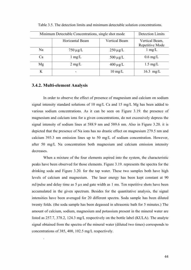
Table 3.5. The detection limits and minimum detectable solution concentrations.
Minimum Detectable Concentrations, single shot mode Detection Limits
Horizantal Beam Vertical Beam Vertical Beam, Repetitive Mode
Na 750 g/L 250 g/L 1 mg/L
Ca 1 mg/L 500 g/L 0.6 mg/L
Mg 2 mg/L 400 g/L 1.5 mg/L
K - 10 mg/L 16.3 mg/L
3.4.2. Multi-element Analysis
In order to observe the effect of presence of magnesium and calcium on sodium
signal intensity standard solutions of 10 mg/L Ca and 15 mg/L Mg has been added to
various sodium concentrations. As it can be seen on Figure 3.19. the presence of
magnesium and calcium ions for a given concentrations, do not excessively depress the
signal intensity of sodium lines at 588.9 nm and 589.6 nm. Also in Figure 3.20. it is
depicted that the presence of Na ions has no drastic effect on magnesium 279.5 nm and
calcium 393.3 nm emission lines up to 50 mg/L of sodium concentration. However,
after 50 mg/L Na concentration both magnesium and calcium emission intensity
decreases.
When a mixture of the four elements aspired into the system, the characteristic
peaks have been observed for those elements. Figure 3.19. represents the spectra for the
drinking soda and Figure 3.20. for the tap water. These two samples both have high
levels of calcium and magnesium. The laser energy has been kept constant at 90
mJ/pulse and delay time as 5 s and gate width as 1 ms. Ten repetitive shots have been
accumulated in the given spectrum. Besides for the quantitative analysis, the signal
intensities have been averaged for 20 different spectra. Soda sample has been diluted
twenty folds. (the soda sample has been degassed in ultrasonic bath for 5 minutes.) The
amount of calcium, sodium, magnesium and potassium present in the mineral water are
listed as 257.7, 378.2, 124.3 mg/L respectively on the bottle label (KULA). The analyte
signal obtained from the spectra of the mineral water (diluted two times) corresponds to
concentrations of 385, 400, 102.5 mg/L respectively.
.
44
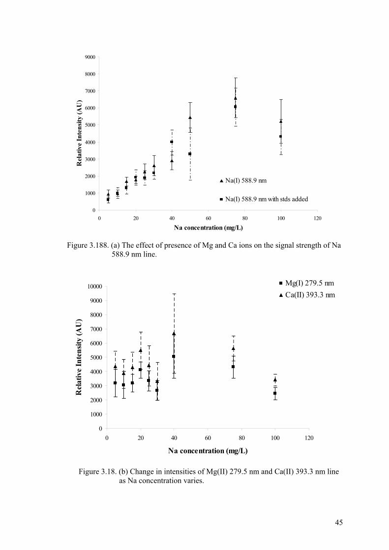
0
1000
2000
3000
4000
5000
6000
7000
8000
9000
0 20 40 60 80 100 120
Na concentration (mg/L)
Rel
ativ
e In
ten
sity
(A
U)
Na(I) 588.9 nm
Na(I) 588.9 nm with stds added
Figure 3.188. (a) The effect of presence of Mg and Ca ions on the signal strength of Na 588.9 nm line.
0
1000
2000
3000
4000
5000
6000
7000
8000
9000
10000
0 20 40 60 80 100 120
Na concentration (mg/L)
Rel
ativ
e In
ten
sity
(A
U)
Mg(I) 279.5 nm
Ca(II) 393.3 nm
Figure 3.18. (b) Change in intensities of Mg(II) 279.5 nm and Ca(II) 393.3 nm line as Na concentration varies.
45

3.4.3. Airborne Concentration
When the aqueous solutions are aspired into the system their concentration may
be expressed as airborne concentration using Equation 3.1. The abbreviations in the
formula stand for the following parameters: c , airborne concentration; Cs, aqueous
solution concentration; rn, nebulizer uptake rate; Sr, sample efficiency, rA carrier gas
flow rate; ρ, density of ambient air.
*
**
A
rn
r
SrCsc
3.2.
Using Equation 3.2, the airborne concentration of the analyte produced by the
pneumatic nebulizer may be calculated. The lowest detectable solution concentration for
horizontal beam set-up is 750 ppb Na+ and corresponds to 374 fg/gr air.
46

Ca (II)
2 5 0 3 5 0 5 5 0 6 5 0 7 0 0 7 5 0 8 0 0 8 5 00
5 0 0 0
1 0 0 0 0
1 5 0 0 0
2 0 0 0 0
2 5 0 0 0
3 0 0 4 0 0 6 0 0
Rel
ativ
e In
tens
ity
(AU
)
w ave len g th (n m )
Figure 3.19. Spectra of mineral water (diluted 20 times) (E=90 mJ, td= 5s tg=1ms, 10 shot accumulation in repetitive mode)
H (I)
N (I)
O (I)
Mg (II)
278.0 278.5 279.0 279.5 280.0 280.5 281.0 281.5 282.00
500
1000
1500
2000
2500
3000
390 392 394 396 398 4000
1000
2000
3000
4000
5000
6000
7000
Na (I)
586 587 588 589 590 591 5920
500
1000
1500
2000
2500
3000
N (I)
47
47

48
200 300 400 500 600 700 800 9000
5000
10000
15000
20000
25000
30000
35000
40000
N (I)
Figure 3.20. Spectra of tap water (E=90 mJ, td= 5s tg=1ms, 10 shot accumulation in repetitive mode)
N (I)
H (I)
Rel
ativ
e In
tens
ity(
AU
)
w avelength (nm )
278 279 280 281 2820
2000
4000
6000
587 588 589 590 591 5920
1000
2000
3000
4000
5000
6000
Mg (II)
Ca (II)
390 391 392 393 394 395 396 397 3980
5000
10000
15000
20000
25000
30000
35000
Na (I)
48

3.4.3. Particle Size
Particle size measurements of the 100 ppm Na aerosols have been determined
using Malvern Mastersizer HD2000. The portable set-up has been attached to the
particle size analyzer. The flow of the aerosols has been kept constant and continuous
during the measurements. The solution has been carried out with two different air and
argon, to see the effect of sample gas density on particle size. When 100 ppm Na
solution carried with air the d50 of the particles were 1.2 m in diameter (d90=4.5 m).
Nevertheless, when sample has been carried with argon the d50 of the aerosol particles
were 1.08 m (d90=4.3 m). When the generated aerosols have passed through a single
naphion, there has been a decrease observed on the particle size. The 50% of the
particles were in range of 0.2 m (d90= 0.5m) when carried by air and argon gases.
Table 3.4 summarizes the size measurement results. The particle size of aerosols has
been decreased by 10 times when membrane dryer has been used. It has been also
observed in enhancement of analyte signal.
Table 3.6. Particle size measurements.
Particle Size (d90) (m)
without membrane dryer with membrane dryer
air argon air argon
4.53 4.29 0.5 0.5
49
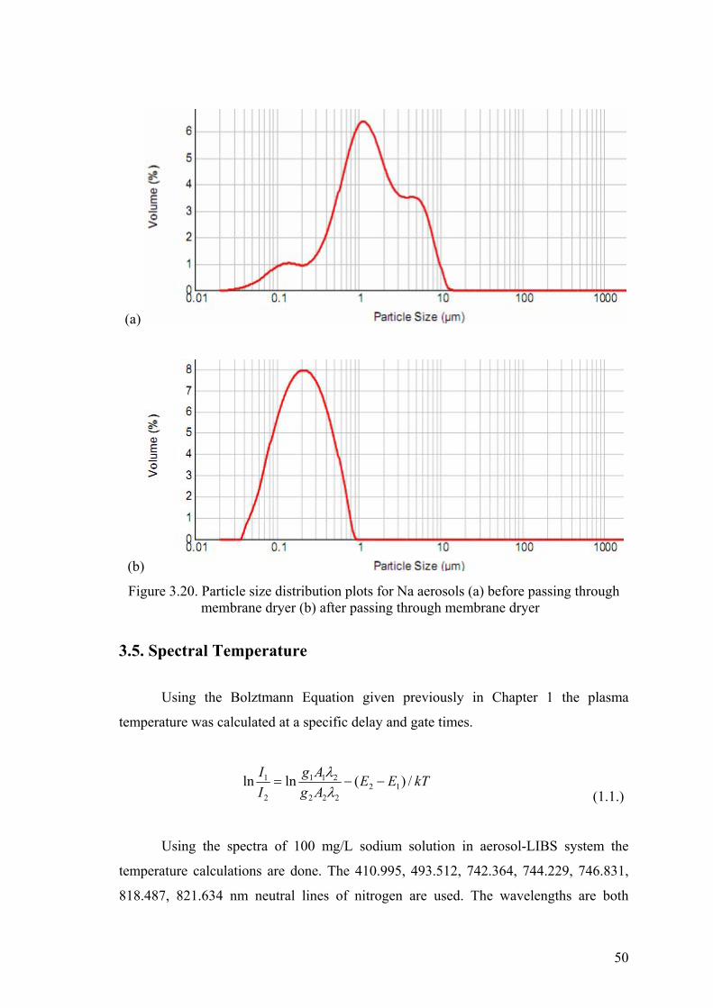
(a)
(b)
Figure 3.20. Particle size distribution plots for Na aerosols (a) before passing through membrane dryer (b) after passing through membrane dryer
3.5. Spectral Temperature
Using the Bolztmann Equation given previously in Chapter 1 the plasma
temperature was calculated at a specific delay and gate times.
kTEEAg
Ag
I
I/)(lnln 12
222
211
2
1
(1.1.)
Using the spectra of 100 mg/L sodium solution in aerosol-LIBS system the
temperature calculations are done. The 410.995, 493.512, 742.364, 744.229, 746.831,
818.487, 821.634 nm neutral lines of nitrogen are used. The wavelengths are both
50
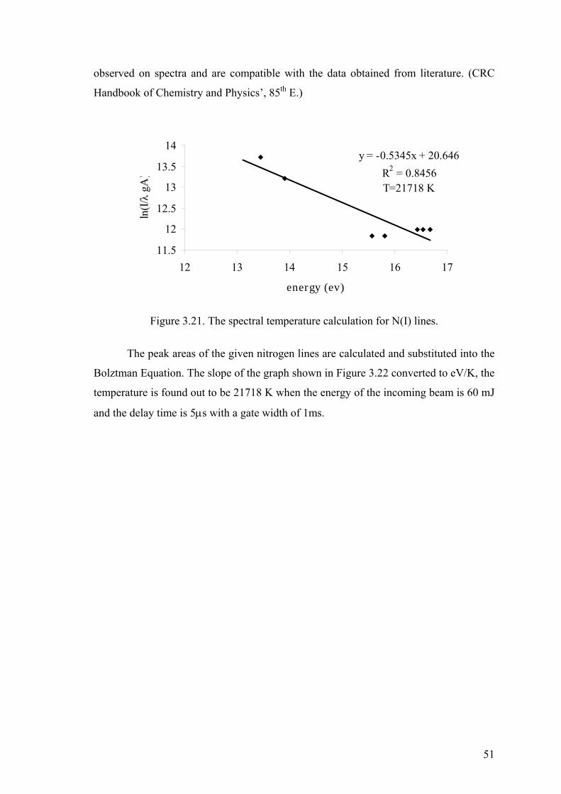
observed on spectra and are compatible with the data obtained from literature. (CRC
Handbook of Chemistry and Physics’, 85th E.)
y = -0.5345x + 20.646
R2 = 0.8456T=21718 K
11.5
12
12.5
13
13.5
14
12 13 14 15 16 17
energy (ev)
ln(I
/λ g
A)
Figure 3.21. The spectral temperature calculation for N(I) lines.
The peak areas of the given nitrogen lines are calculated and substituted into the
Bolztman Equation. The slope of the graph shown in Figure 3.22 converted to eV/K, the
temperature is found out to be 21718 K when the energy of the incoming beam is 60 mJ
and the delay time is 5s with a gate width of 1ms.
51

CHAPTER 4
CONCLUSION
In this study, an aerosol generation system has been designed, constructed and
coupled to a LIBS system that has been set-up from the commercially available parts.
Pneumatic nebulization method has been used to generate particles and a special
heating/cooling and membrane drying steps are conjuncted.
Two different experimental LIBS set-up, horizontal and telescopic, were used to
form plasma. In telescopic setup, in which the laser beam has been directed from the top
of the sample chamber, the plasma image is formed vertically along the slit height of the
spectrograph. This way, the variation in plasma position on the slit due to shot to shot
variation of the laser pulses has been reduced. The experimental parameters such as
flow rate, heating and cooling temperatures, delay times, gate widths, detector gain and
laser energies have been optimized for sodium, calcium, magnesium and potassium
elements.
Sodium, calcium, magnesium and potassium elements have been studied and the
detection limits have been found to be 1, 0.6, 1.5 and 16.3 mg/L respectively. These
values for detection limits are comparable to the values given in literature. Besides, real
samples mineral water and tap water have been analyzed. Also standard addition of
calcium and magnesium on sodium element has shown that the sodium analyte is not
highly affected by the presence of the matrix elements.
The efficiency of the heating/cooling unit and the membrane dryer has been
demonstrated. 90 % of the aqueous analyte solution has been converted into aerosol.
Particle size measurements have been performed. The particles size range has been
found as 4.3 m for sodium. The membrane dryer has reduced the particle size of
aerosol droplets to 0.5 m.
52

REFERENCES
Aglio M., Colao F., Fantoni R., Lazic V. 2005. Double-pulse LIBS in bulk water and on submerged bronze samples. Applied Surface Science 247: 157–162.
Band Yehuda. Light and Matter. Wiley, England , 2006. Caceres J. O., Lopez J. T., Telle H.H., Urena A.G. 2001. Quantitative analysis of trace
metal ions in ice using laser-induced breakdown spectroscopy. Spectrochimica Acta Part B 56: 831-838.
Cheng M., Martin M. 2000. Detection of Chromium Aerosol Using Time-Resolved
Laser-Induced Plasma Spectroscopy. Applied Spectroscopy 54: 1279-1285. Cremers D.A., Radziemski L.J. Handbook of Laser-Induced Breakdown Spectroscopy.
John&Willey Sons Ltd. England, 2006. Gautier C., Fichet P., Menut D., Lacour J., Hermite D. 2004. Study of the double-pulse
setup with an orthogonal beam geometry for laser-induced breakdown spectroscopy. Spectrochimica Acta Part B 59: 975–986.
Gondal M. A., Hussain T. 2007. Determination of poisonous metals in wastewater
collected from paint manufacturing plant using laser-induced breakdown spectroscopy, Talanta 71: 73-80.
Griem, H., Haines M. G. Principles of Plasma Spectroscopy. McGraw-Hill, 1964. Demidov A., Andrews D. An Introduction to Laser Spectroscopy. Springer. 2006. Hahn D. W., Hohreiter V. 2006. Plasma-Particle Interactions in a Laser-Induced
Plasma: Implications for Laser-Induced Breakdown Spectroscopy. Anal.Chem. 78: 1509-1514.
Hahn D.W. Carranza J.E. 2001. Aerosol generation systems for development and
calibration of laser induced breakdown spectroscopy instrumentation. Review of Scientific Instruments 72: 3706-3713.
Hahn D.W. Carranza J.E. 2001. On-line analysis of ambient air aerosols using laser-
induced breakdown spectroscopy. Spectrochimica Acta Part B 56: 851-864. Hahn D.W., Asgill M. E. 2009. Particle Size Limits for Quantitative Aerosol Analysis
Using Laser-induced Breakdown Spectroscopy: Temporal Considerations. Spectrochimica Acta PartB 64: 1153-1158.
Hahn D.W., Diwakar P.K., Jackson P.B. (2007) The effect of multi-component aerosol
particles on quantitative laser-induced breakdown spectroscopy: Considerations of localized matrix effects. Spectrochimica Acta Part B 62: 1466-1474.
53
Hahn D.W., Diwakar P.K. Windom B.C. 2006. Dual-pulse Laser Induced Breakdown Spectroscopy for Analysis of Gaseous and Aerosol Systems: Plasma-analyte interactions. Spectrochimica Acta Part B 61: 788-796.
Hahn D.W., Lunden M. M. 2000. Detection and analysis of aerosol particles by laser-
induced breakdown spectroscopy. Aerosol Science and Technology 33: 30-48. Harith M.A., Charfi B. 2002. Panoramic laser-induced breakdown spectrometry of
water. Spectrochimica Acta A Part B 57, 1141-1153. What’s naphion? Perma Pure LLC http://www.permapure.com/industry/science/technology/?ind=science (Accessed on June 2010). Three Four Level Lasers http://www.unc.edu/~dtmoore/3_4level.html (Accessed on June 2010). Huang J., Liu H., Lin K. 2006. Laser-induced breakdown spectroscopy in analysis of
Al+3 liquid droplets: On-line preconcentration by use of flow injection. Analytica Chimica Acta 581. 303-308.
Janzen C. Fleige R. Noll R. 2005. Analysis of small droplets with a new detector for
liquid chromatography based on laser-induced breakdown spectroscopy. Spectrochimica Acta Part B 60: 993-1001.
Koch S., Garen W., Müller M., Neu W. 2004. Detection of chromium in liquids by laser
induced breakdown spectroscopy (LIBS). Appl. Phys A 79: 1071-1073. Laserna J.J., Palanco S., Alises A., Cunat J., Baena J. 2003. Development of a portable
laser-induced plasma spectrometer with fully-automated operation and quantitative analysis capabilities. Journal of Analytical Atomic Spectrometry (18) 933-938.
Laserna J.J., Trujillo L.A., Ferrero A. 2008. Preliminary studies of stand-off laser
induced breakdown spectroscopy detection of aerosols. Journal of Analytical Atomic Spectrometry 23: 885-888.
Lazic V., Colao F., Fantoni R., Spizzicchino V. 2005. Laser-induced breakdown
spectroscopy in water: Improvement of the detection threshold by signal processing. Spectrochimica Acta Part B 60: 1002–1013.
Lazic V., Jovicenic S., Fantoni R., Colao F. 2007. Efficient plasma and bubble
generation underwater by an optimized laser excitation and its application for liquid analyses by laser-induced breakdown spectroscopy. Spectrochimica Acta Part B 62: 1433–1442.
Lin K., Binke C., Huang J. 2004. Matrix effect on emission current correlated analysis
in laser-induced breakdown spectroscopy of liquid droplets. Spectrochimica Acta Part B 59: 321–326.
54
55
Mohamed Y. Tawfik W. 2008. Improved LIBS limit of detection of Be, Mg, Si, Mn, Fe and Cu in aluminum alloy samples using a portable Echelle spectrometer with ICCD camera. Optics&LaserTechnology 40: 30–38.
Molina A., Shaddic C., Sickafoose S., Walsh P. Blevins L. 2005. Effect of temperature
and CO2 concentration on laser-induced breakdown spectroscopy measurements of alkali fume. Spectrochimica Acta Part B 60: 1103–1114.
NIST Atomic Spectra Database Lines Form (Accessed on June 2010)
http://physics.nist.gov/PhysRefData/ASD/lines_form.html. Onge L., Kwong E.,Sabsabi M., Vadas E. 2004. Rapid analysis of liquid formulations
containing sodium chloride using laser-induced breakdown spectroscopy. Journal of Pharmaceutical and Biomedical Analysis 36: 277–284.
Panne U., Neuhausser R. E., Theisen M., Fink H., Niessner R. 2001. Analysis of heavy
metal aerosols on filters by laser induced plasma spectroscopy. Spectrochimica acta Part B 56: 839-850.
Radziemski L. J., Essien M. 1988. Detection of Cadmium, Lead and Zinc in Aerosols
by Laser-induced Breakdown Spectroometry. Journal of Analytical Atomic Spectrometry 3: 985-988.
Radziemski L. J., Loree R. T., Cremers D. A., Hoffman N. M. 1983. Time resolved
Laser-Induced Breakdown Spectrometry of Aerosols. Analytical Chemistry 55: 1246-1252.
Radziemski L.J., Cremers D.A., Loree T.R. 1984. Spectrochemical Analysis of Liquids
Using the Laser Spark. Applied Spectroscopy 38: 721-729 Unal. S., Yalcin S. 2010. Development of a continuous flow hydride generation laser-
induced breakdown spectroscopic system: Determination of tin in aqueous environments. Spectrochimica Acta Part B 65: 750–757.
Yaroshchyk P., Morrison R., Body D., Chadwick B. L. 2005. Quantitative
determination of wear metals in engine oils using laser-induced breakdown spectroscopy: A comparison between liquid jets and static liquids. Spectrochimica Acta Part B 60: 986-992.
Yoshiro I., Nakamura S., Sone K. 1996. Determination of an Iron Suspension in Water
by Laser-Induced Breakdown Spectroscopy with Two Sequential Laser Pulses. Analytical Chemistry 68: 2981-2986.


