LARGE DATA AND ZERO NOISE LIMITS OF GRAPH-BASED1
SEMI-SUPERVISED LEARNING ALGORITHMS ∗2
MATTHEW M. DUNLOP † , DEJAN SLEPCEV ‡ , ANDREW M. STUART § , AND3
MATTHEW THORPE ¶4
Abstract. Scalings in which the graph Laplacian approaches a differential operator in the5
large graph limit are used to develop understanding of a number of algorithms for semi-supervised6
learning; in particular the extension, to this graph setting, of the probit algorithm, level set and7
kriging methods, are studied. Both optimization and Bayesian approaches are considered, based8
around a regularizing quadratic form found from an affine transformation of the Laplacian, raised9
to a, possibly fractional, exponent. Conditions on the parameters defining this quadratic form are10
identified under which well-defined limiting continuum analogues of the optimization and Bayesian11
semi-supervised learning problems may be found, thereby shedding light on the design of algorithms12
in the large graph setting. The large graph limits of the optimization formulations are tackled13
through Γ−convergence, using the recently introduced TLp metric. The small labelling noise limit14
of the Bayesian formulations are also identified, and contrasted with pre-existing harmonic function15
approaches to the problem.16
Key words. Semi-supervised learning, Bayesian inference, higher-order fractional Laplacian,17
asymptotic consistency, kriging.18
AMS subject classifications. 62G20, 62C10, 62F15, 49J5519
1. Introduction.20
1.1. Context. This paper is concerned with the semi-supervised learning prob-21
lem of determining labels on an entire set of (feature) vectors xjj∈Z , given (possibly22
noisy) labels yjj∈Z′ on a subset of feature vectors with indices j ∈ Z ′ ⊂ Z. To be23
concrete we will assume that the xj are elements of Rd, d ≥ 2, and consider the binary24
classification problem in which the yj are elements of ±1. Our goal is to characterize25
algorithms for this problem in the large data limit where n = ∣Z ∣ → ∞; additionally26
we will study the limit where the noise in the label data disappears. Studying these27
limits yields insight into the classification problem and algorithms for it.28
Semi-supervised learning as a subject has been developed primarily over the last29
two decades and the references [51, 52] provide an excellent source for the historical30
context. Graph based methods proceed by forming a graph with n nodes Z, and use31
the unlabelled data xjj∈Z to provide an n × n weight matrix W quantifying the32
affinity of the nodes of the graph with one another. The labelling information on Z ′33
is then spread to the whole of Z, exploiting these affinities. In the absence of labelling34
information we obtain the problem of unsupervised learning; for example the spectrum35
of the graph Laplacian L forms the basis of widely used spectral clustering methods36
[3, 34, 45]. Other approaches are combinatorial, and largely focussed on graph cut37
methods [8, 9, 36]. However relaxation and approximation are required to beat the38
combinatorial hardness of these problems [31] leading to a range of methods based39
on Markov random fields [30] and total variation relaxation [40]. In [52] a number40
∗Submitted to the editors May 2018.†Computing and Mathematical Sciences, Caltech, Pasadena, CA 91125 ([email protected] )‡Department of Mathematical Sciences, Carnegie Mellon University, Pittsburgh, PA 15213
([email protected])§Computing and Mathematical Sciences, Caltech, Pasadena, CA 91125 ([email protected] ).¶Department of Applied Mathematics and Theoretical Physics, University of Cambridge, Cam-
bridge, CB3 0WA ([email protected])
1
of new approaches were introduced, including label propagation and the generaliza-41
tion of kriging, or Gaussian process regression [47], to the graph setting [53]. These42
regression methods opened up new approaches to the problem, but were limited in43
scope because the underlying real-valued Gaussian process was linked directly to the44
categorical label data which is (arguably) not natural from a modelling perspective;45
see [33] for a discussion of the distinctions between regression and classification. The46
logit and probit methods of classification [48] side-step this problem by postulating a47
link function which relates the underlying Gaussian process to the categorical data,48
amounting to a model linking the unlabelled and labelled data. The support vector49
machine [7] makes a similar link, but it lacks a natural probabilistic interpretation.50
The probabilistic formulation is important when it is desirable to equip the clas-51
sification with measures of uncertainty. Hence, we will concentrate on the probit52
algorithm in this paper, and variants on it, as it has a probabilistic formulation.53
The statement of the probit algorithm in the context of graph based semi-supervised54
learning may be found in [6]. An approach bridging the combinatorial and Gaussian55
process approaches is the use of Ginzburg-Landau models which work with real num-56
bers but use a penalty to constrain to values close to the range of the label data ±1;57
these methods were introduced in [4], large data limits studied in [15, 42, 44], and58
given a probabilistic interpretation in [6]. Finally we mention the Bayesian level set59
method. This approach takes the idea of using level sets for inversion in the class of60
interface problems [11] and gives it a probabilistic formulation which has both theo-61
retical foundations and leads to efficient algorithms [28]; classification may be viewed62
as an interface problem on a graph (a graph cut is an interface for example) and thus63
the Bayesian level set method is naturally extended to this setting as shown in [6].64
As part of this paper we will show that the probit and Bayesian level set methods are65
closely related.66
A significant challenge for the field, both in terms of algorithmic development,67
and in terms of fundamental theoretical understanding, is the setting in which the68
volume of unlabelled data is high, relative to the volume of labelled data. One way69
to understand this setting is through the study of large data limits in which n = ∣Z ∣→70
∞. This limit is studied in [46], and was addressed more recently under different71
assumptions in [21]. Both papers assume that the unlabelled data is drawn i.i.d.72
from a measure with Lebesgue density on a subset of Rd, but the assumptions on73
graph construction differ: in [46] the graph bandwidth is fixed as n → ∞ resulting74
in the limit of the graph Laplacian being a non-local operator, whilst in [21] the75
bandwidth vanishes in the limit resulting in the limit being a weighted Laplacian76
(divergence form elliptic operator).77
In [32] it is demonstrated that algorithms based on use of the discrete Dirichlet78
energy computed from the graph Laplacian can behave poorly for d ≥ 2, in the large79
data limit, if they attempt pointwise labelling. In [50] it is argued that use of quadratic80
forms based on powers α > d2
of the graph Laplacian can ameliorate this problem.81
Our work, which studies a range of algorithms all based on optimization or Bayesian82
formulations exploiting quadratic forms, will take this body of work considerably83
further, proving large data limit theorems for a variety of algorithms, and showing84
the role of the parameter α in this infinite data limit. In doing so we shed light85
on the difficult question of how to scale and tune algorithms for graph based semi-86
supervised learning; in particular we state limit theorems of various kinds which87
require, respectively, either α > d2
or α > d to hold. We also study the small noise88
limit and show how both the probit and Bayesian level set algorithms coincide and,89
furthermore, provide a natural generalization of the harmonic functions approach of90
2

[53, 54], a generalization which is arguably more natural from a modeling perspective.91
Our large data limit theorems concern the maximum a posteriori (MAP) estimator92
rather than a Bayesian posterior distribution. However two remarkable recent papers93
[20, 19] demonstrate a methodology for proving limit theorems concerning Bayesian94
posterior distributions themselves, exploiting the variational characterization of Bayes95
theorem; extending the work in those papers to the algorithms considered in this paper96
would be of great interest.97
1.2. Our Contribution. We derive a canonical continuum inverse problem98
which characterizes graph based semi-supervised learning: find function u ∶ Ω ⊂ Rd ↦99
R from knowledge of sign(u) on Ω′ ⊂ Ω. 1 The latent variable u characterizes the100
unlabelled data and its sign is the labelling information. This highly ill-posed inverse101
problem is potentially solvable because of the very strong prior information provided102
by the unlabelled data; we characterize this information via a mean zero Gaussian103
process prior on u with covariance operator C ∝ (L + τ2I)−α. The operator L is a104
weighted Laplacian found as a limit of the graph Laplacian, and as a consequence105
depends on the distribution of the unlabelled data.106
In order to derive this canonical inverse problem we study the probit and Bayesian107
level set algorithms for semi-supervised learning. We build on the large unlabelled108
data limit setting of [21]. In this setting there is an intrinsic scaling parameter εn that109
characterizes the length scale on which edge weights between nodes are significant;110
the analysis identifies a lower bound on εn which is necessary in order for the graph111
to remain connected in the large data limit and under which the graph Laplacian112
L converges to a differential operator L of weighted Laplacian form. The work uses113
Γ−convergence in the TL2 optimal transport metric, introduced in [21], and proves114
convergence of the quadratic form defined by L to one defined by L. We make the115
following contributions which significantly extend this work to the semi-supervised116
learning setting.117
We prove Γ−convergence in TL2 of the quadratic form defined by (L+ τ2I)α118
to that defined by (L + τ2I)α and identify parameter choices in which the119
limiting Gaussian measure with covariance (L + τ2I)−α is well-defined. See120
Theorems 1, 4 and Proposition 5.121
We introduce large data limits of the probit and Bayesian level set problem122
formulations in which the volume of unlabelled data n = ∣Z ∣ → ∞, distin-123
guishing between the cases where the volume of labelled data ∣Z ′∣ is fixed and124
where ∣Z ′∣/n is fixed. See section 4 for the function space analogues of the of125
the graph based algorithms introduced in section 3.126
We use the theory of Γ−convergence to derive a continuum limit of the probit127
algorithm when employed in MAP estimation mode; this theory demonstrates128
the need for α > d2
and an upper bound on εn in the large data limit where129
the volume of labelled data ∣Z ′∣ is fixed. See Theorems 10 and 11130
We use the properties of Gaussian measures on function spaces to write down131
well defined limits of the probit and Bayesian level set algorithms, when em-132
ployed in Bayesian probabilistic mode, to determine the posterior distribution133
on labels given observed data; this theory demonstrates the need for α > d2
in134
order for the limiting probability distribution to be meaningful for both large135
data limits; indeed, depending on the geometry of the domain from which the136
feature vectors are drawn, it may require α > d for the case where the volume137
1 We note that throughout the paper Ω is the physical domain, and not the set of events of aprobability space.
3
of labelled data is fixed. See Theorem 4 and Proposition 5 for these condi-138
tions on α, and for details of the limiting probability measures see equations139
(21), (22), (23) and (24).140
We show that the probit and Bayesian level set method have a common141
Bayesian inverse problem limit, mentioned above, by studying their weak142
limits as noise levels on the label data tends to zero. See Theorems 8 and 14.143
We provide numerical experiments which illusrate the large graph limits in-144
troduced and studied in this paper; see section 5.145
1.3. Paper Structure. In section 2 we study a family of quadratic forms which146
arise naturally in all the algorithms that we study. By means of the Γ−convergence147
techniques pioneered in [21] we show that these quadratic forms have a limit defined148
by families of differential operators in which the finite graph parameters appear in an149
explicit and easily understood fashion. Section 3 is devoted to the definition of the150
three graph based algorithms that we study in this paper: the probit and Bayesian151
level set algorithms, and the graph analogue of kriging. In section 4 we write down the152
function space limits of these algorithms, obtained when the volume n of unlabelled153
data tends to infinity, and in the case of the maximum a posteriori estimator for154
probit use Γ−convergence to study large graph limits rigorously; we also show that155
the probit and Bayesian level set algorithms have a common zero noise limit. Section 5156
contains numerical experiments for the function space limits of the algorithms, in both157
optimization (MAP) and sampling (fully Bayesian MCMC) modalities. We conclude158
in section 6 with a summary and directions for future research. All proofs are given159
in the Appendix, section 7. This choice is made in order to separate the form and160
implications of the theory from the proofs; both the statements and proofs comprise161
the contributions of this work, but since they may be of interest to different readers162
they are separated, by use of the Appendix.163
2. Key Quadratic Form and Its Limits.164
2.1. Graph Setting. From the unlabelled data xjnj=1 we construct a weighted165
graph G = (Z,W ) where Z = 1,⋯, n are the vertices of the graph and W the edge166
weight matrix; W is assumed to have entries wij between nodes i and j given by167
wij = ηε(∣xi − xj ∣).
We will discuss choice of the function ηε ∶ R ↦ R+ in detail below; heuristically it168
should be thought of as proportional to a mollified Dirac mass, or a characteristic169
function of a small interval. From W we construct the graph Laplacian as follows.170
We define the diagonal matrix D = diagdii with entries dii = ∑j∈Z wij . We can then171
define the unnormalized graph Laplacian L =D −W . Our results may be generalized172
to the normalized graph Laplacian L = I −D− 12WD− 1
2 and we will comment on this173
in the conclusions.174
2.2. Quadratic Form. We view u ∶ Z ↦ R as a vector in Rn and define the175
quadratic form176
⟨u,Lu⟩ = 1
2∑i,j∈Z
wij ∣u(i) − u(j)∣2;
here ⟨⋅, ⋅⟩ denotes the standard Euclidean inner-product on Rn. This is the discrete177
Dirichlet energy defined via the graph Laplacian L and appears as a basic quantity178
in many unsupervised and semi-supervised learning algorithms. In this paper our179
4
interest focusses on forms based on powers of L:180
J(α,τ)n (u) = 1
2n⟨u,A(n)u⟩
where, for τ ≥ 0 and α > 0,181
(1) A(n) = (snL + τ2I)α.
The sequence parameters sn will be chosen appropriately to ensure that the quadratic182
form J(α,τ)n (u) converges to a well-defined limit as n→∞.183
In addition to working in a set-up which results in a well-defined limit, we will184
also ask that this limit results in a quadratic form defined by a differential operator.185
This, of course, requires some form of localization and we will encode this as follows:186
we will assume that ηε(⋅) = ε−dη(⋅/ε), inducing a Dirac mass approximation as ε→ 0;187
later we will discuss how to relate ε to n. For now we state the assumptions on η that188
we employ throughout the paper:189
Assumptions 1 (on η). The edge weight profile function η satisfies:190
(K1) η(0) > 0 and η(⋅) continuous at 0;191
(K2) η non-increasing;192
(K3) ∫∞
0 η(r)rd+1dr <∞;193
Notice that assumption (K3) implies that194
(2) ση ∶=1
d∫Rdη(∣h∣)∣h∣2dh <∞ and βη ∶= ∫
Rdη(∣h∣)dh <∞.
A notable fact about the limits that we study in the remainder of the paper is that195
they depend on η only through the constants ση, βη, provided Assumptions 1 hold196
and ε = εn and sn are chosen as appropriate functions of n.197
2.3. Limiting Quadratic Form.198
The limiting quadratic form is defined on an open and bounded set Ω ⊂ Rd.199
Assumptions 2 (on Ω). We assume that Ω is a connected, open and bounded200
subset of Rd. We also assume that Ω has C1,1boundary. 2201
Assumptions 3 (on density ρ). We assume that n feature vectors xj ∈ Ω are202
sampled i.i.d. from a probability measure µ supported on Ω with smooth Lebesgue203
density ρ bounded above and below by finite strictly positive constants ρ± uniformly204
on Ω.205
We index the data by Z = 1,⋯, n and let Ωn = xii∈Z be the data set. This206
data set induces the empirical measure207
µn =1
n∑i∈Z
δxi .
2The assumption that Ω is connected is not essential but makes stating the results simpler. Weremark that a number of the results, and in particular the convergence of Theorem 1, hold if we onlyassume that the boundary of Ω is Lipschitz. We need the stronger assumption in order to be able toemploy elliptic regularity to characterize functions in fractional Sobolev spaces, see Section 2.4 andLemma 16; this is essential to be able to define Gaussian measures on function spaces, and thereforeneeded to define a Bayesian approach in which uncertainty of classifiers may be estimated.
5
Given a measure ν on Ω we define the weighted Hilbert space L2ν = L2
ν(Ω;R) with208
inner-product209
(3) ⟨a, b⟩ν = ∫Ωa(x)b(x)ν(dx)
and induced norm defined by the identity ∥ ⋅ ∥2L2ν= ⟨⋅, ⋅⟩ν . Note that with these defini-210
tions we have211
J(α,τ)n ∶ L2µn ↦ [0,+∞), J(α,τ)n (u) = 1
2⟨u,A(n)u⟩µn .
In what follows we apply a form of Γ−convergence to establish that for large n the212
quadratic form J(α,τ)n is well approximated by the limiting quadratic form213
J(α,τ)∞ ∶ L2µ ↦ [0,+∞) ∪ +∞, J(α,τ)∞ (u) = 1
2⟨u,Au⟩µ.
Here µ is the measure on Ω with density ρ, and we define the L2µ self-adjoint differential214
operator L by215
(4) Lu = −1
ρ∇ ⋅ (ρ2∇u), x ∈ Ω,
∂u
∂n= 0, x ∈ ∂Ω.
The operator A is then defined by A = (L + τ2I)α.216
We may now relate the quadratic forms defined by A(n) and A. The TL2 topology217
is introduced in [21] and defined in the Appendix section 7.2.2 for convenience. The218
following theorem is proved in section 7.4.219
Theorem 1. Let Assumptions 1–3 hold. Let α > 0, εnn=1,2,... be a positive220
sequence converging to zero, and such that221
(5)
limn→∞
( logn
n)
1/d 1
εn= 0 if d ≥ 3,
limn→∞
( logn
n)
1/2 (logn) 14
εn= 0 if d = 2,
and assume that the scale factor sn is defined by222
(6) sn =2
σηnε2n
.
Then, with probability one, we have223
1. Γ- limn→∞ J(α,τ)n = J(α,τ)∞ with respect to the TL2 topology;224
2. if τ = 0, any sequence un with un ∶ Ωn → R satisfying supn ∥un∥L2µn
< ∞225
and supn∈N J(α,0)n (un) <∞ is pre-compact in the TL2 topology;226
3. if τ > 0, any sequence un with un ∶ Ωn → R satisfying supn∈N J(α,τ)n (un) <∞227
is pre-compact in the TL2 topology.228
Remark 2. As we discuss in section 7.2.1 of the appendix, Γ-convergence and pre-229
compactness allow one to show that minimizers of a sequence of functionals converge230
to the minimizer of the limiting functional. The results of Theorem 1 provide the231
Γ-convergence and pre-compactness of fractional Dirichlet energies, which are the key232
term of the functionals, such as (10) below, that define the learning algorithms that we233
study. In particular Theorem 1 enables us to prove the convergence, in the large data234
limit n → ∞, of minimizers of functionals such as (10) (i.e. of outcomes of learning235
algorithms), as shown in Theorem 10.236
6
2.4. Function Spaces. The operator L given by (4) is uniformly elliptic as a237
consequence of the assumptions on ρ, and is self-adjoint with respect to the inner238
product (3) on L2µ. By standard theory, it has a discrete spectrum: 0 = λ1 < λ2 ≤ ⋯,239
where the fact that 0 < λ2 uses the connectedness of the domain and the uniform240
positivity of ρ on the domain. Let ϕi for i = 1, . . . be the associated L2µ-orthonormal241
eigenfunctions. They form a basis of L2µ.242
By Weyl’s law the eigenvalues of λjj≥1 of L satisfy λj ≍ j2/d. For completeness a243
simple proof is proved in Lemma 27; the analogous and more general results applicable244
to the Laplace-Beltrami operator may be found in, Hormander [27].245
Spectrally defined Sobolev spaces. For s ≥ 0 we define246
Hs(Ω) = u ∈ L2µ ∶
∞∑k=1
λska2k <∞
where ak = ⟨u,ϕk⟩µ and thus u = ∑k akϕk in L2µ. We note that Hs(Ω) is a Hilbert247
space with respect to the inner product248
⟪u, v⟫s,µ = a1b1 +∞∑k=1
λskakbk
where bk = ⟨v,ϕk⟩µ. It follows from the definition that for any s ≥ 0, Hs(Ω) is249
isomorphic to a weighted `2(N) space, where the weights are formed by the sequence250
1, λs2, λs3, . . . .251
In Lemma 16 in the Appendix section 7.1 we show that for any integer s >252
0, Hs(Ω) ⊂ Hs(Ω) where Hs(Ω) is the standard fractional Sobolev space. More253
precisely we characterize Hs(Ω) as the set of those functions in Hs(Ω) which satisfy254
the appropriate boundary condition and show that the norms of Hs(Ω) and Hs(Ω)255
are equivalent on Hs(Ω).256
We also note that for any integer s and θ ∈ (0,1) the space Hs+θ is a interpolation257
space between Hs and Hs+1. In particular Hs+θ = [Hs,Hs+1]θ,2, where the real258
interpolation space used is as in Definition 3.3 of Abels [1]. This identification of259
Hs follows from the characterization of interpolation spaces of weighted Lp spaces by260
Peetre [35], as referenced by Gilbert [24]. Together these facts allow us to characterize261
the Holder regularity of functions in Hs(Ω).262
Lemma 3. Under Assumptions 2–3, for all s ≥ 0 there exists a bounded, linear,263
extension mapping E ∶ Hs(Ω) → Hs(Rd). That is for all f ∈ Hs(Ω), E(f)∣Ω = f a.e.264
Furthermore:265
(i) if s < d2
then Hs(Ω) embeds continuously in Lq(Ω) for any q ≤ 2dd−2s
;266
(ii) if s > d2
then Hs(Ω) embeds continuously in C0,γ(Ω) for any γ < min1, s− d2.267
The proof is presented in the Appendix 7.1.268
We note that this implies that when α > d2
pointwise evaluation is well-defined in269
the limiting quadratic form J(α,τ)∞ ; this will be used in what follows to show that the270
the limiting labelling model obtained when ∣Z ′∣ is fixed is well-posed.271
2.5. Gaussian Measures of Function Spaces. Using the ellipticity of L,272
Weyl’s law, and Lemma 3 allows us to characterize the regularity of samples of Gaus-273
sian measures on L2µ. The proof of the following theorem is a straightforward ap-274
plication of the techniques in [17, Theorem 2.10] to obtain the Gaussian measures275
on Hs(Ω). Concentration of the measure on Hs and on C0,γ(Ω) then follows from276
7
Lemma 3. When τ = 0 we work on the space orthogonal to constants in order that C277
(defined in the theorem below) is well defined.278
Theorem 4. Let Assumptions 2–3 hold. Let L be the operator defined in (4),279
and define C = (L + τ2I)−α. For any fixed α > d2
and τ ≥ 0, the Gaussian measure280
N(0,C) is well-defined on L2µ. Draws from this measure are almost surely in Hs(Ω)281
for any s < α − d2
, and consequently in C0,γ(Ω) for any γ < min1, α − d if α > d.282
We note that if the operator L has eigenvectors which are as regular as those of283
the Laplacian on a flat torus then the conclusions of Theorem 4 can be strengthened.284
Namely if in addition to what we know about L, there is C > 0 such that285
(7) supj≥1
(∥ϕj∥L∞ + 1
j1/dLip(ϕj)) ≤ C,
then the Kolmogorov continuity technique [17, Section 7.2.5] can be used to show286
additional Holder continuity.287
Proposition 5. Let Assumptions 2–3 hold. Assume the operator L satisfies con-288
dition (7) and define C = (L + τ2I)−α. For any fixed α > d/2 and τ ≥ 0, the Gaussian289
measure N(0,C) is well-defined on L2µ. Draws from this measure are almost surely in290
Hs(Ω;R) for any s < α − d/2, and in C0,γ(Ω;R) for any γ < min1, α − d2 if α > d
2.291
We note that in general one cannot expect that the operator L satisfies the bound292
(7). For example, for the ball there is a sequence of eigenfunctions which satisfy293
∥ϕk∥L∞ ∼ λ(d−1)/4k ∼ k(d−2)/(2d), see [25]. In fact this is the largest growth of eigen-294
functions possible, as on general domains with smooth boundary ∥ϕk∥L∞ ≲ λ(d−1)/4k ,295
as follows from the work of Grieser, [25]. Analogous bounds have first been estab-296
lished for operators on manifolds without boundary by Hormander, [27]. This bound297
is rarely saturated as shown by Sogge and Zeldtich [39], but determining the scaling298
for most sets and manifolds remains open. Establishing the conditions on Ω under299
which the Theorem 4 can be strengthened as in Proposition 5 is of great interest.300
3. Graph Based Formulations. We now assume that we have access to label301
data defined as follows. Let Ω′ ⊂ Ω and let Ω± be two subsets of Ω′ such that302
Ω+ ∪Ω− = Ω′, Ω+ ∩Ω− = ∅.
We will consider two labelling scenarios:303
Labelling Model 1. ∣Z ′∣/n → r ∈ (0,∞). We assume that Ω± have positive304
Lebesgue measure. We assume that the xjj∈N are drawn i.i.d. from measure305
µ. Then if xj ∈ Ω+ we set yj = 1 and if xj ∈ Ω− then yj = −1. The label306
variables yj are not defined if xj ∈ Ω/Ω′ where Ω′ = Ω+ ∪ Ω−. We assume307
dist(Ω+,Ω−) > 0 and define Z ′ ⊂ Z to be the subset of indices for which we308
have labels.309
Labelling Model 2. ∣Z ′∣ fixed as n → ∞. We assume that Ω± comprise a310
fixed number of points, n± respectively. We assume that the xjj>n++n− are311
drawn i.i.d. from measure µ whilst xj1≤j≤n+ are a fixed set of points in312
Ω+ and xjn++1≤j≤n++n− are a fixed set of points in Ω−. We label these fixed313
points by y ∶ Ω± ↦ ±1 as in Labelling Model 1. We define Z ′ ⊂ Z to be314
the subset of indices 1,⋯, n++n− for which we have labels and Ω′ = Ω+∪Ω−.315
In both cases j ∈ Z ′ if and only if xj ∈ Ω′. But in Model 1 the xj are drawn i.i.d. and316
assigned labels when they lie in Ω′, assumed to have positive Lebesgue measure; in317
8
Model 2 the (xj , yj)j∈Z′ are provided, in a possibly non-random way, independently318
of the unlabelled data.319
We will identify u ∈ Rn and u ∈ L2µn(Ω;R) by uj = u(xj) for each j ∈ Z. Similarly,320
we will identify y ∈ Rn++n− and y ∈ L2µn(Ω
′;R) by yj = y(xj) for each j ∈ Z ′. We may321
therefore write, for example,322
1
n⟨u,Lu⟩Rn = ⟨u,Lu⟩µn
where u is viewed as a vector on the left-hand side and a function on Z on the323
right-hand side.324
The algorithms that we study in this paper have interpretations through bothoptimization and probability. The labels are found from a real-valued function u ∶Z ↦ R by setting y = S u ∶ Z ↦ R with S the sign function defined by
S(0) = 0; S(u) = 1, u > 0; and S(u) = −1, u < 0.
The objective function of interest takes the form
J(n)(u) = 1
2⟨u,A(n)u⟩µn + rnΦ(n)(u).
The quadratic form depends only on the unlabelled data, while the function Φ(n) is325
determined by the labelled data. Choosing rn = 1n
in Labeling Model 1 and rn = 1326
in Labeling Model 2 ensures that the total labelling information remains of O(1) in327
the large n limit. Probability distributions constructed by exponentiating multiples328
of J(n)(u) will be of interest to us; the probability is then high where the objective329
function is small, and vice-versa. Such probabilities represent the Bayesian posterior330
distribution on the conditional random variable u∣y.331
3.1. Probit. The probit algorithm on a graph is defined in [6] and here gener-332
alized to a quadratic form based on A(n) rather than L. We define333
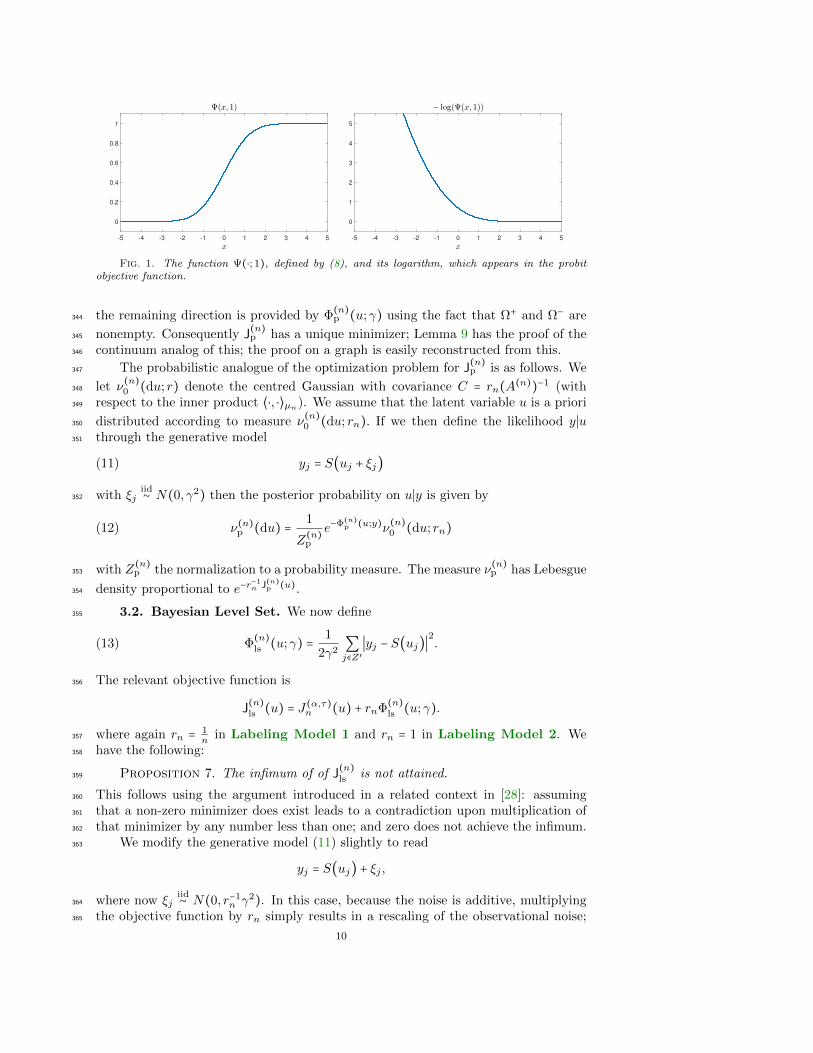
(8) Ψ(v;γ) = 1√2πγ2
∫v
−∞exp ( − t2/2γ2)dt
and then334
(9) Φ(n)p (u;γ) = − ∑j∈Z′
log(Ψ(yjuj ;γ)).
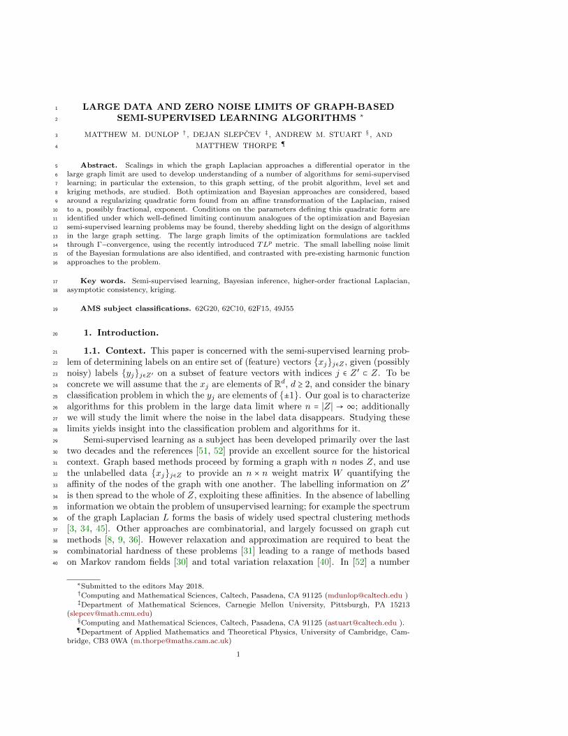
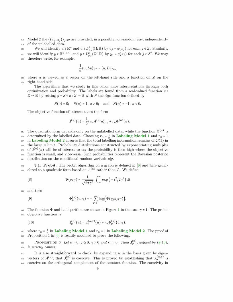
The function Ψ and its logarithm are shown in Figure 1 in the case γ = 1. The probit335
objective function is336
(10) J(n)p (u) = J(α,τ)n (u) + rnΦ(n)p (u;γ).
where rn = 1n
in Labeling Model 1 and rn = 1 in Labeling Model 2. The proof of337
Proposition 1 in [6] is readily modified to prove the following.338
Proposition 6. Let α > 0, τ ≥ 0, γ > 0 and rn > 0. Then J(n)p , defined by (8-10),339
is strictly convex.340
It is also straightforward to check, by expanding u in the basis given by eigen-341
vectors of A(n), that J(n)p is coercive. This is proved by establishing that J
(α,τ)n is342
coercive on the orthogonal complement of the constant function. The coercivity in343
9
-5 -4 -3 -2 -1 0 1 2 3 4 5
0
0.2
0.4
0.6
0.8
1
-5 -4 -3 -2 -1 0 1 2 3 4 5
0
1
2
3
4
5
Fig. 1. The function Ψ(⋅; 1), defined by (8), and its logarithm, which appears in the probitobjective function.
the remaining direction is provided by Φ(n)p (u;γ) using the fact that Ω+ and Ω− are344
nonempty. Consequently J(n)p has a unique minimizer; Lemma 9 has the proof of the345
continuum analog of this; the proof on a graph is easily reconstructed from this.346
The probabilistic analogue of the optimization problem for J(n)p is as follows. We347
let ν(n)0 (du; r) denote the centred Gaussian with covariance C = rn(A(n))−1 (with348
respect to the inner product ⟨⋅, ⋅⟩µn). We assume that the latent variable u is a priori349
distributed according to measure ν(n)0 (du; rn). If we then define the likelihood y∣u350
through the generative model351
(11) yj = S(uj + ξj)
with ξjiid∼ N(0, γ2) then the posterior probability on u∣y is given by352
(12) ν(n)p (du) = 1
Z(n)p
e−Φ(n)p (u;y)ν(n)0 (du; rn)
with Z(n)p the normalization to a probability measure. The measure ν
(n)p has Lebesgue353
density proportional to e−r−1n J(n)p (u).354
3.2. Bayesian Level Set. We now define355
(13) Φ(n)ls (u;γ) = 1
2γ2 ∑j∈Z′
∣yj − S(uj)∣2.
The relevant objective function is356
J(n)ls (u) = J(α,τ)n (u) + rnΦ
(n)ls (u;γ).
where again rn = 1n
in Labeling Model 1 and rn = 1 in Labeling Model 2. We357
have the following:358
Proposition 7. The infimum of of J(n)ls is not attained.359
This follows using the argument introduced in a related context in [28]: assuming360
that a non-zero minimizer does exist leads to a contradiction upon multiplication of361
that minimizer by any number less than one; and zero does not achieve the infimum.362
We modify the generative model (11) slightly to read363
yj = S(uj) + ξj ,
where now ξjiid∼ N(0, r−1
n γ2). In this case, because the noise is additive, multiplying364
the objective function by rn simply results in a rescaling of the observational noise;365
10
multiplication by rn does not have such a simple interpretation in the case of pro-366
bit. As a consequence the resulting Bayesian posterior distribution has significant367
differences with the probit case: the latent variable u is now assumed a priori to be368
distributed according to measure ν(n)0 (du; 1) Then369
(14) ν(n)ls (du) = 1
Z(n)ls
e−rnΦ(n)ls(u;γ)ν
(n)0 (du; 1)
where ν(n)0 is the same centred Gaussian as in the probit case. Note that ν
(n)ls is also370
the measure with Lebesgue density proportional to e−J(n)ls(u).371
3.3. Small Noise Limit. When the size of the noise on the labels is small,372
the probit and Bayesian level set approaches behave similarly. More precisely, the373
measures ν(n)p and ν
(n)ls share a common weak limit as γ → 0. The following result374
is given without proof – this is because its proof is almost identical to that arising375
in the continuum limit setting of Theorem 14(ii) given in the appendix; indeed it is376
technically easier due to the fully discrete setting. Here ⇒ denotes weak convergence377
of probability measures.378
Theorem 8. Let ν(n)0 (du) denote a Gaussian measure of the form ν
(n)0 (du; r)
for any r, possibly depending on n. Define the set
Bn = u ∈ Rn ∣ yjuj > 0 for each j ∈ Z ′
and the probability measure
ν(n)(du) = Z−11Bn(u)ν(n)0 (du)
where Z = ν(n)0 (Bn). Consider the posterior measures ν(n)p defined in (12) and ν
(n)ls379
defined in (14). Then ν(n)p ⇒ν(n) and ν
(n)ls ⇒ν(n) as γ → 0.380
3.4. Kriging. Instead of classification, where the sign of the latent variable u is381
made to agree with the labels, one can alternatively consider regression where u itself382
is made to agree with the labels [53, 54]. We consider this situation numerically in383
section 5. Here the objective is to384
minimize J(n)k (u) ∶= J(α,τ)n (u) subject to u(xj) = yj for all j ∈ Z ′.
In the continuum setting this minimization is referred to as kriging, and we extend385
the terminology to our graph based setting. Kriging may also be defined in the case386
where the constraint is enforced as a soft least squares penalty; however we do not387
discuss this here.388
The probabilistic analogue of this problem can be linked with the original work389
of Zhu et al [53, 54] which based classification on a centred Gaussian measure with390
inverse covariance given by the graph Laplacian, conditioned to take the value exactly391
1 on labelled nodes where yj = 1, and to take the value exactly −1 on labelled nodes392
where yj = −1.393
4. Function Space Limits of Graph Based Formulations. In this section394
we state Γ−limit theorems for the objective functions appearing in the probit algo-395
rithm. The proofs are given in the appendix. They rely on arguments which use396
the fact that we study perturbations of the Γ−limit theorem for the quadratic forms397
11
stated in section 2. We also write down formal infinite dimensional formulations of398
the probit and Bayesian level set posterior distributions, although we do not prove399
that these limits are attained. We do, however, show that the probit and level set400
posteriors have a common limit as γ → 0, as they do on a finite graph.401
4.1. Probit. Under Labelling Model 1, the natural continuum limit of the402
probit objective functional is403
(15) Jp(v) = J(α,τ)∞ (v) +Φp,1(v;γ)
where404
(16) Φp,1(v;γ) = −∫Ω′
log(Ψ(y(x)v(x);γ))dµ(x)
for a given measurable function y ∶ Ω′ → ±1. For any v ∈ L2µ, log(Ψ(y(x)v(x);γ))405
is integrable by Corollary 26. The proof of the following theorem is given in the406
appendix, in section 7.5.407
Lemma 9. Let Assumptions 1–3 hold. For α ≥ 1 and τ ≥ 0, consider the functional408
Jp with Labelling Model 1 defined by (15). Then, the functional Jp has a unique409
minimizer in Hα(Ω).410
Proof. Convexity of Jp follows from the proof of Proposition 1 in [6]. Let v+ and411
v− be the averages of v on Ω+ and Ω− respectively. Namely let v± = 1∣Ω±∣ ∫Ω±
v(x)dx.412
Note that413
Jp(v) ≥ J(α,τ)∞ (v) ≥ λα−12 J(1,0)∞ (v) = −1
2λα−1
2 ∫Ωv∇ ⋅ (ρ2∇v)dx ≥ (ρ−)2λα−1
2
2∥∇v∥2
L2(Ω).
Using the form of Poincare inequality given in Theorem 13.27 of [29] implies that414
(17) Jp(v) ≳ ∥∇v∥2L2(Ω) ≳ ∫
Ω∣v − v+∣2 + ∣v − v−∣2 dx.
The convexity of Φp,1(v;γ) implies that415
Φp,1(v;γ) ≥ − log(Ψ(v+);γ)µ(Ω+) − log(Ψ(−v−);γ)µ(Ω−)
Using that lims→−∞ − log(Ψ(s;γ)) =∞ we see that a bound on Φp,1(v;γ) provides a416
lower bound on v+ and an upper bound on v−. To see this let Θ be the inverse of417
s↦ − log(Ψ(s;γ)). The preceding shows that418
v+ ≥ Θ(Φp,1(v;γ)µ(Ω+)
) ≥ Θ( Jp(v)µ(Ω+)
) and v− ≤ −Θ(Φp,1(v;γ)µ(Ω−)
) ≤ −Θ( Jp(v)µ(Ω−)
) .
Let c = max−Θ ( Jp(v)µ(Ω+)) ,−Θ ( Jp(v)
µ(Ω−)) ,0. Then v+ ≥ −c and v− ≤ c. Using that, for
any a ∈ R, v2 ≤ 2∣v − a∣2 + 2a2, we obtain
∫Ωv2(x)dx ≤ ∫v(x)≤−c v
2(x)dx + ∫v(x)≥c v2(x)dx + c2∣Ω∣
≤ 2∫v(x)≤−c ∣v + c∣2 + c2 dx + 2∫v(x)≥c ∣v − c∣
2 + c2 dx + c2∣Ω∣
≤ 5c2∣Ω∣ + 2∫v(x)≤−c ∣v − v+∣2 dx + 2∫v(x)≥c ∣v − v−∣
2 dx
≲ c2∣Ω∣ + Jp(v).12
Then ∥v∥L2 is bounded by a function of Jp(v) and Ω.419
Combining with (17) implies that a function of Jp(v) bounds ∥v∥2Hα(Ω) which420
establishes the coercivity of Jp. The functional Jp is weakly lower-somicontinuous in421
Hα, due to convexity of both J(α,τ)∞ and Φp,1. Thus the direct method of the calculus422
of variations proves that Jp has a unique minimizer in Hα(Ω).423
The following theorem is proved in section 7.5.424
Theorem 10. Let the assumptions of Labelling Model 1 and Theorem 1 hold425
with τ ≥ 0. Then, with probability one, any sequence of minimizers vn of J(n)p converge426
in TL2 to v∞, the unique minimizer of Jp in L2µ, and furthermore limn→∞ J
(n)p (vn) =427
Jp(v∞) = minv∈L2µJp(v).428
The analogous result under Labelling Model 2, i.e. convergence of minimizers,429
is an open question. In this case the natural continuum limit of the probit objective430
functional is431
(18) Jp(v) = J(α,τ)∞ (v) +Φp,2(v;γ)
where432
(19) Φp,2(v;γ) = − ∑j∈Z′
log(Ψ(y(xj)u(xj);γ)
for a given measurable function y ∶ Ω′ → ±1. When α ≤ d2
this limiting model433
is not well-posed. In particular the regularity of the functional is not sufficient to434
impose pointwise data. More precisely, when α ≤ d2
then there exists a sequence of435
smooth functions vk ∈ C∞(Ω) such that limk→∞ Jp(vk) = 0. In particular when α < d2,436
consider a smooth, compactly supported, mollifier ζ, with ζ(0) > 0 and define vk(x) =437
ck∑Ni=1 y(xi)ζ1/k(x − xi) where ck → ∞ sufficiently slowly. Then Φp,2(vk;γ) → 0 as438
k → ∞ and, by a simple scaling argument (for appropriate ck), J(α,τ)∞ (vk) → 0 as439
k →∞. Another way to see that the problem is not well defined is that the functions440
in Hα(Ω) (which is the natural space to consider Jp on) are not continuous in general441
and evaluating Φp,2(v;γ) is not well defined.442
When α > d2
the existence of minimizers of (18) in Hα(Ω) is established by the443
direct method of the calculus of variations using the convexity of Jp and the fact that,444
by Lemma 3, Hα continuously embeds into a set of Holder continuous functions.445
For α > d2
we believe that the minimizers of Jnp of Labelling Model 2 converge446
to minimizers of (18) in an appropriate regime, but the situation is more complicated447
than for Labelling Model 1: under Labelling Model 2 (5) is no longer a sufficient448
condition on the scaling of ε with n for the convergence to hold. Thus if ε → 0 too449
slowly the problem degenerates. In particular in the following theorem we identify450
the asymptotic behavior of minimizers of Jp both when α < d2, and if α > d
2but ε→ 0451
too slowly.452
The proof of the following may be found in section 7.6. The theorem is similar453
in spirit to Proposition 2.2(ii) in [38] where a similar phenomenon was discussed454
for the p-Laplacian regularized semi-supervised learning. We also mention that the455
PDE approach to a closely related p-Laplacian problem was recently introduced by456
Calder [12].457
Theorem 11. Let the assumptions of Labelling Model 2, and Theorem 1 hold.458
If α > d2
, τ > 0, and459
(20) εnn12α →∞ as n→∞
13

or if α < d2
then, with probability one, the sequence of minimizers vn of J(n)p converge460
to 0 in TL2 as n →∞. That is, the minimizers of J(n)p converge to the minimizer of461
J(α,τ)∞ with the information about the labels being lost in the limit.462
Remark 12. We believe, but do not have a proof, that for α > d2
and τ > 0, if463
εnn12α → 0 as n→∞
then, with probability one, any sequence of minimizers vn of J(n)p is sequentially464
compact in TL2 with limn→∞ J(n)p (vn) = minv∈L2
µJp(v) given by (18), (19). If this465
holds then, under Labelling Model 2, J(n)p (u) converges in an appropriate sense to466
a limiting objective function Jp(u). Our numerical results support this conjecture.467
It is also of interest to consider the limiting probability distributions which arise468
under the two labelling models. Under Labelling Model 2 this density has, in physi-469
cist’s notation, “Lebesgue density” exp(−Jp(u)). Under Labelling Model 1, how-470
ever, we have shown that J(n)p (u) converges in an appropriate sense to a limiting objec-471
tive function Jp(u) implying that (again in physicist’s notation) exp(−r−1n J
(n)p (u)) ≈472
exp(−nJp(u)). Thus under Labelling Model 1 the posterior probability concen-473
trates on a Dirac measure at the minimizer of Jp(u).474
Based on this remark, the natural continuum probability limit concerns La-475
belling Model 2. The posterior probability is then given by476
(21) νp,2(du) =1
Zp,2e−Φp,2(u;γ)ν0(du)
where ν0 is the centred Gaussian with covariance C given in Theorem 4 and Φp,2 is477
given by (19). Since we require pointwise evaluation to make sense of Φp,2(u;γ) we,478
in general, require α > d; however Proposition 5 gives conditions under which α > d2
479
will suffice. We will also consider the probability measure νp,1 defined by480
(22) νp,1(du) =1
Zp,1e−Φp,1(u;γ)ν0(du)
where Φp,1 is given by (16). The function Φp,1(u;γ) is defined in an L2µ sense and481
thus we require only α > d2
– see Theorem 4. Note, however, that this is not the482
limiting probability distribution that we expect for Labelling Model 1 with the483
parameter choices leading to Theorem 10 since the argument above suggests that this484
will concentrate on a Dirac. However we include the measure νp,1 in our discussions485
because, as we will show, it coincides with the analogous Bayesian level set measure486
νls,1 (defined below) in the small observational noise limit. Since νls,1 can be obtained487
by a natural scaling of the graph algorithm, which does not concentrate on Dirac,488
the relationship between νp,1 and νls,1 is of interest as they are both, for small noise,489
relaxations of the same limiting object.490
4.2. Bayesian Level Set. We now study probabilistic analogues of the Bayesianlevel set method, again using the measure ν0 which is the centred Gaussian withcovariance C given in Theorem 4 for some α > d
2. Note that, from equation (13), for
14
Labelling Model 1,
rnΦ(n)ls (u;γ) = 1
2γ2
1
n∑j∈Z′
∣y(xj) − S(u(xj))∣2
≈ ∫Ω′
1
2γ2∣y(x) − S(u(x))∣2 dµ(x)
∶= Φls,1(u;γ)
by a law of large numbers type argument of the type underlying the proof of Theorem491
10.492
Recall that, from the discussion following Proposition 7, this scaling corresponds493
to employing the finite dimensional Bayesian level set model with observational vari-494
ance γ2n so that the variance per observation is constant. Then the natural limiting495
probability measure is, in physicists notation, exp(−Jls(u)) where496
Jls(u) = J(α,τ)∞ (u) +Φls,1(u;γ).
Expressed in terms of densities with respect to the Gaussian prior this gives497
(23) νls,1(du) =1
Zls,1e−Φls,1(u;γ)ν0(du).
Since Φls,1(u;γ) makes sense in L2µ we require only α > d
2. The measure νls,1 is the498
natural analogue of the finite dimensional measure ν(n)ls under this label model. Under499
Labelling Model 2 we take rn = 1. We obtain a measure νls,2 in the form (23) found500
by replacing νls,1 by νls,2 and Φls,1 by501
(24) Φls,2(u;γ) ∶= ∑j∈Z′
1
2γ2∣y(xj) − S(u(xj))∣
2.
In this case the observational variance is not-rescaled by n since the total number of502
labels is fixed. Since we require pointwise evaluation to make sense of Φls,2(u;γ) we,503
in general, require α > d; however Proposition 5 gives conditions under which α > d2
504
will suffice.505
Remark 13. Note that J(n)ls and Jls cannot be connected via Γ-convergence. In-506
deed, if Jls = Γ- limn→∞ J(n)ls then Jls would be lower semi-continuous [10]. When507
τ > 0 compactness of minimizers follows directly from the compactness property of508
the quadratic forms J(α,τ)n , see Theorem 1. Now since compactness of minimizers plus509
lower semi-continuity implies existence of minimizers then the above reasoning implies510
there exists minimizers of Jls. But as in the discrete case, Proposition 7, multiplying511
any u by a constant less than one leads to a smaller value of Jls. Hence the infimum512
cannot be achieved. It follows that Jls ≠ Γ- limn→∞ J(n)ls .513
4.3. Small Noise Limit. As for the finite graph problems, the labeled data canbe viewed as arising from different generative models. In the probit formulation, thegenerative models for the labels are given by
y(x) = S(u(x) + ξ(x)), ξ ∼ N(0, γ2I),
y(xj) = S(u(xj) + ξj), ξjiid∼ N(0, γ2).
15
for Labelling Model 1, Labelling Model 2 respectively; S is the sign function.The functionals Φp,1, Φp,2 then arise as the negative log-likelihoods from these models.Similarly, in the Bayesian level set formulation the generative models are given by
y(x) = S(u(x)) + ξ(x), ξ ∼ N(0, γ2I),
y(xj) = S(u(xj)) + ξj , ξjiid∼ N(0, γ2).
leading to the functionals Φls,1, Φls,2.514
We show that in the zero noise limit the Bayesian level set and probit posterior515
distributions coincide. However for γ > 0 they differ: note, for example, that the516
probit model enforces binary data, whereas the Bayesian level set model does not.517
It has been observed that the Bayesian level set posterior can be used to produce518
similar quality classification to the Ginzburg-Landau posterior, at significantly lower519
computational cost [18]. The small noise limit is important for two reasons: firstly520
in many applications labelling is very accurate and considering the zero noise limit is521
therefore instructive; secondly recent work [5] shows that the zero noise limit provides522
useful information about the efficiency of algorithms applied to sample the posterior523
distribution and, in particular, constants derived from the zero noise limit appear524
in lower bounds on average acceptance probability and mean square jump in such525
algorithms.526
Proof of the following is given in section 7.7.527
Theorem 14.528
(i) Let Assumptions 2–3 hold, and assume that α > d. Let the assumptions of529
Labelling Model 1 hold. Define the set530
B∞,1 = u ∈ C(Ω;R) ∣ y(x)u(x) > 0 for a.e. x ∈ Ω′
and the probability measure
ν1(du) = Z−11B∞,1(u)ν0(du)
where Z = ν0(B∞,1). Consider the posterior measures νp,1 defined in (22) and531
νls,1 defined in (23). Then νp,1⇒ν1 and νls,1⇒ν1 as γ → 0.532
(ii) Let Assumptions 2–3 hold, and assume that α > d. Let the assumptions of533
Labelling Model 2 hold. Define the set534
B∞,2 = u ∈ C(Ω;R) ∣ y(xj)u(xj) > 0 for each j ∈ Z ′
and the probability measure
ν2(du) = Z−11B∞,2(u)ν0(du)
where Z = ν0(B∞,2). Then νp,2⇒ν2 and νls,2⇒ν2 as γ → 0.535
Remark 15. The assumption that α > d in both parts of the above theorem can536
be relaxed to α > d/2 if the conclusions of Proposition 5 are satisfied.537
4.4. Kriging. One can define kriging in the continuum setting [47] analogously538
to the discrete setting; we consider this numerically in section 5. In the case of539
Labelling Model 2, the limiting problem is to540
minimize Jk(u) ∶= J(α,τ)∞ (u) subject to u(xj) = yj for all j ∈ Z ′.
Kriging may also be defined for Labelling Model 1 and without the hard constraint541
in the continuum setting, but we do not discuss either of these scenarios here.542
16
0 0.2 0.4 0.6 0.8 1
0
0.2
0.4
0.6
0.8
1
0 0.2 0.4 0.6 0.8 1
0
0.2
0.4
0.6
0.8
1
0 0.2 0.4 0.6 0.8 1
0
0.2
0.4
0.6
0.8
1
0 0.2 0.4 0.6 0.8 1
0
0.2
0.4
0.6
0.8
1
0 0.2 0.4 0.6 0.8 1
0
0.2
0.4
0.6
0.8
1
Fig. 2. The cross sections of the data densities ρh we consider in subsection 5.1.
5. Numerical Illustrations. In this section we describe the results of numerical543
experiments which illustrate or extend the developments in the preceding sections.544
In section 5.1 we study the effect of the geometry of the data on the classification545
problem, by studying an illustrative example in dimension d = 2. Section 5.2 studies546
how the relationship between the length-scale ε and the graph size n affects limiting547
behaviour. In section 5.3 we study graph based kriging. Finally, in section 5.4, we548
study continuum problems from the Bayesian perspective, studying the quantification549
of uncertainty in the resulting classification.550
5.1. Effect of Data Geometry on Classification. We study how the ge-551
ometry of the data affects the classification under Labelling Model 1, using the552
continuum probit model. Let Ω = (0,1)2. We first consider a uniform distribution ρ553
on the domain, and choose Ω+,Ω− to be balls of radius 0.05 centred at (0.25,0.25),554
(0.75,0.75) respectively. The decision boundary is then naturally the perpendicular555
bisector of the line segment joining the centers of these balls. We then modify ρ by556
introducing a channel of increasing depth in ρ dividing the domain in two vertically,557
and look at how this affects the decision boundary. Specifically, given h ∈ [0,1] we558
define ρh to be constant in the y-direction, and assume the cross-sections in the x-559
direction are as shown in Figure 2, so that the channel has depth 1 − h. In order to560
numerically estimate the continuum probit minimizers, we construct a finite-difference561
approximation to each L on a uniform grid of 65536 points, which then provides an562
approximation to A. The objective function J(∞)p is then minimized numerically using563
the linearly-implicit gradient flow method described in [6], Algorithm 4.564
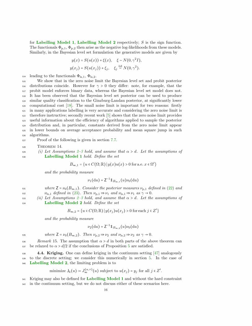
We consider both the effect of the channel depth parameter h and the parameter565
α on the classification; we fix τ = 10 and γ = 0.01. In Figure 3 we show the minimizers566
arising from 5 different choices of h and α = 1,2,3. As the depth of the channel is in-567
creased, the minimizers begin to develop a jump along the channel. As α is increased,568
the minimizers become less localized around the labelled regions, and the jump along569
the channel becomes sharper as a result. Note that the scale of the minimizers de-570
creases as α increases. This could formally be understood from a probabilistic point571
of view: under the prior we have E∥u∥2L2 = Tr(A−1) ≍ τ−2α, and so a similar scaling572
may be expected to hold for the MAP estimators. In Figure 4 we show the sign of573
each minimizer in Figure 3 to illustrate the resulting classifications. As the depth of574
the channel is increased, the decision boundary moves continuously from the diagonal575
to the vertical bisector of the domain, with the transitional boundaries appearing al-576
most as a piecewise linear combination of both boundaries. We also see that, despite577
the minimizers themselves differing significantly for different α, the classifications are578
almost invariant with respect to α.579
17
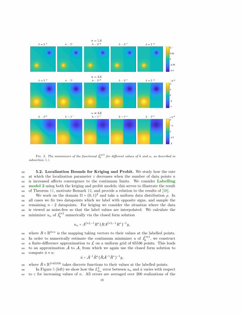
Fig. 3. The minimizers of the functional J(∞)p for different values of h and α, as described in
subsection 5.1.
5.2. Localization Bounds for Kriging and Probit. We study how the rate580
at which the localization parameter ε decreases when the number of data points n581
is increased affects convergence to the continuum limits. We consider Labelling582
model 2 using both the kriging and probit models; this serves to illustrate the result583
of Theorem 11, motivate Remark 12, and provide a relation to the results of [38].584
We work on the domain Ω = (0,1)2 and take a uniform data distribution ρ. In585
all cases we fix two datapoints which we label with opposite signs, and sample the586
remaining n − 2 datapoints. For kriging we consider the situation where the data587
is viewed as noise-free so that the label values are interpolated. We calculate the588
minimizer un of J(n)k numerically via the closed form solution589
un = A(n),−1R∗(RA(n),−1R∗)−1y,
where R ∈ R2×n is the mapping taking vectors to their values at the labelled points.590
In order to numerically estimate the continuum minimizer u of J(∞)k , we construct591
a finite-difference approximation to L on a uniform grid of 65536 points. This leads592
to an approximation A to A, from which we again use the closed form solution to593
compute u ≈ u:594
u = A−1R∗(RA−1R∗)−1y,
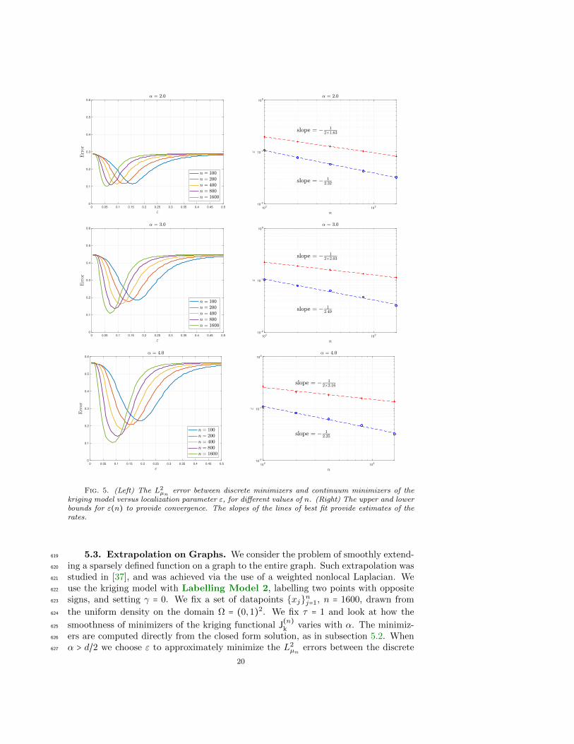
where R ∈ R2×65556 takes discrete functions to their values at the labelled points.595
In Figure 5 (left) we show how the L2µn error between un and u varies with respect596
to ε for increasing values of n. All errors are averaged over 200 realizations of the597
18
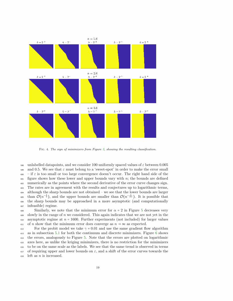
Fig. 4. The sign of minimizers from Figure 3, showing the resulting classification.
unlabelled datapoints, and we consider 100 uniformly spaced values of ε between 0.005598
and 0.5. We see that ε must belong to a ‘sweet-spot’ in order to make the error small599
– if ε is too small or too large convergence doesn’t occur. The right hand side of the600
figure shows how these lower and upper bounds vary with n; the bounds are defined601
numerically as the points where the second derivative of the error curve changes sign.602
The rates are in agreement with the results and conjectures up to logarithmic terms,603
although the sharp bounds are not obtained – we see that the lower bounds are larger604
than O(n− 12 ), and the upper bounds are smaller than O(n− 1
2α ). It is possible that605
the sharp bounds may be approached in a more asymptotic (and computationally606
infeasible) regime.607
Similarly, we note that the minimum error for α = 2 in Figure 5 decreases very608
slowly in the range of n we considered. This again indicates that we are not yet in the609
asymptotic regime at n = 1600. Further experiments (not included) for larger values610
of n show that the minimum error does converge as n→∞ as expected.611
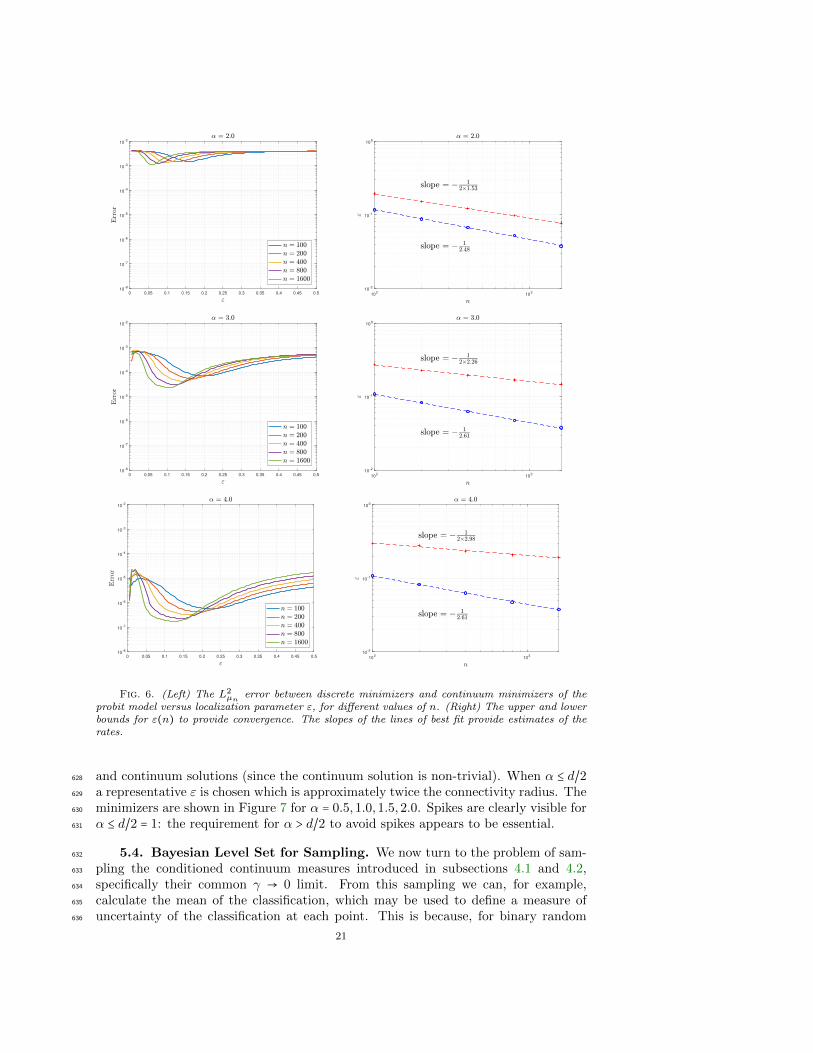
For the probit model we take γ = 0.01 and use the same gradient flow algorithm612
as in subsection 5.1 for both the continuum and discrete minimizers. Figure 6 shows613
the errors, analogously to Figure 5. Note that the errors are plotted on logarithmic614
axes here, as unlike the kriging minimizers, there is no restriction for the minimizers615
to be on the same scale as the labels. We see that the same trend is observed in terms616
of requiring upper and lower bounds on ε, and a shift of the error curves towards the617
left as n is increased.618
19
0 0.05 0.1 0.15 0.2 0.25 0.3 0.35 0.4 0.45 0.5
0
0.1
0.2
0.3
0.4
0.5
0.6
102
103
10-2
10-1
100
0 0.05 0.1 0.15 0.2 0.25 0.3 0.35 0.4 0.45 0.5
0
0.1
0.2
0.3
0.4
0.5
0.6
102
103
10-2
10-1
100
0 0.05 0.1 0.15 0.2 0.25 0.3 0.35 0.4 0.45 0.5
0
0.1
0.2
0.3
0.4
0.5
0.6
102
103
10-2
10-1
100
Fig. 5. (Left) The L2µn error between discrete minimizers and continuum minimizers of the
kriging model versus localization parameter ε, for different values of n. (Right) The upper and lowerbounds for ε(n) to provide convergence. The slopes of the lines of best fit provide estimates of therates.
5.3. Extrapolation on Graphs. We consider the problem of smoothly extend-619
ing a sparsely defined function on a graph to the entire graph. Such extrapolation was620
studied in [37], and was achieved via the use of a weighted nonlocal Laplacian. We621
use the kriging model with Labelling Model 2, labelling two points with opposite622
signs, and setting γ = 0. We fix a set of datapoints xjnj=1, n = 1600, drawn from623
the uniform density on the domain Ω = (0,1)2. We fix τ = 1 and look at how the624
smoothness of minimizers of the kriging functional J(n)k varies with α. The minimiz-625
ers are computed directly from the closed form solution, as in subsection 5.2. When626
α > d/2 we choose ε to approximately minimize the L2µn errors between the discrete627
20
0 0.05 0.1 0.15 0.2 0.25 0.3 0.35 0.4 0.45 0.510
-8
10-7
10-6
10-5
10-4
10-3
10-2
102
103
10-2
10-1
100
0 0.05 0.1 0.15 0.2 0.25 0.3 0.35 0.4 0.45 0.510
-8
10-7
10-6
10-5
10-4
10-3
10-2
102
103
10-2
10-1
100
0 0.05 0.1 0.15 0.2 0.25 0.3 0.35 0.4 0.45 0.510
-8
10-7
10-6
10-5
10-4
10-3
10-2
102
103
10-2
10-1
100
Fig. 6. (Left) The L2µn error between discrete minimizers and continuum minimizers of the
probit model versus localization parameter ε, for different values of n. (Right) The upper and lowerbounds for ε(n) to provide convergence. The slopes of the lines of best fit provide estimates of therates.
and continuum solutions (since the continuum solution is non-trivial). When α ≤ d/2628
a representative ε is chosen which is approximately twice the connectivity radius. The629
minimizers are shown in Figure 7 for α = 0.5,1.0,1.5,2.0. Spikes are clearly visible for630
α ≤ d/2 = 1: the requirement for α > d/2 to avoid spikes appears to be essential.631
5.4. Bayesian Level Set for Sampling. We now turn to the problem of sam-632
pling the conditioned continuum measures introduced in subsections 4.1 and 4.2,633
specifically their common γ → 0 limit. From this sampling we can, for example,634
calculate the mean of the classification, which may be used to define a measure of635
uncertainty of the classification at each point. This is because, for binary random636
21
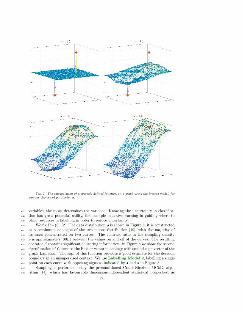
Fig. 7. The extrapolation of a sparsely defined function on a graph using the kriging model, forvarious choices of parameter α.
variables, the mean determines the variance. Knowing the uncertainty in classifica-637
tion has great potential utility, for example in active learning in guiding where to638
place resources in labelling in order to reduce uncertainty.639
We fix Ω = (0,1)2. The data distribution ρ is shown in Figure 8; it is constructed640
as a continuum analogue of the two moons distribution [49], with the majority of641
its mass concentrated on two curves. The contrast ratio in the sampling density642
ρ is approximately 100:1 between the values on and off of the curves. The resulting643
operator L contains significant clustering information: in Figure 8 we show the second644
eigenfunction of L, termed the Fiedler vector in analogy with second eigenvector of the645
graph Laplacian. The sign of this function provides a good estimate for the decision646
boundary in an unsupervised context. We use Labelling Model 2, labelling a single647
point on each curve with opposing signs as indicated by and in Figure 8.648
Sampling is performed using the preconditioned Crank-Nicolson MCMC algo-649
rithm [14], which has favourable dimension-independent statistical properties, as650
22
0
0.5
1
1.5
2
2.5
3
3.5
-2
-1.5
-1
-0.5
0
0.5
1
1.5
2
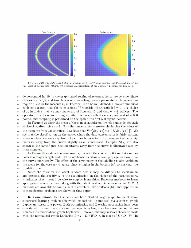
Fig. 8. (Left) The data distribution ρ used in the MCMC experiments, and the locations of thetwo labelled datapoints. (Right) The second eigenfunction of the operator L corresponding to ρ.
demonstrated in [19] in the graph-based setting of relevance here. We consider three651
choices of α > d/2, and two choices of inverse length-scale parameter τ . In general we652
require α > d for the measure ν2 in Theorem 14 to be well-defined. However numerical653
evidence suggests that the conclusions of Proposition 5 are satisfied with this choice654
of ρ, implying that we may make use of Remark 15 and that α > d2
suffices. The655
operator L is discretized using a finite difference method on a square grid of 40000656
points, and sampling is performed on the span of its first 500 eigenfunctions.657
In Figure 9 we show the mean of the sign of samples on the left hand side, for each658
choice of α, after fixing τ = 1. Note that uncertainty is greater the further the values of659
the mean are from ±1: specifically we have that Var(S(u(x)) = 1−[E(S(u(x)))]2. We660
see that the classification on the curves where the data concentrates is fairly certain,661
whereas classification away from the curves is uncertain; furthermore the certainty662
increases away from the curves slightly as α is increased. Samples S(u) are also663
shown in the same figure; the uncertainty away from the curves is illustrated also by664
these samples.665
In Figure 10 we show the same results, but with the choice τ = 0.2 so that samples666
possess a longer length scale. The classification certainty now propagates away from667
the curves more easily. The effect of the asymmetry of the labelling is also visible in668
the mean for the case α = 4: uncertainty is higher in the bottom-left corner than the669
top-left corner.670
Since the prior on the latent random field u may be difficult to ascertain in671
applications, the sensitivity of the classification on the choice of the parameters α,672
τ indicates that it could be wise to employ hierarchical Bayesian methods to learn673
appropriate values for them along with the latent field u. Dimension robust MCMC674
methods are available to sample such hierarchical distributions [13], and application675
to classification problems are shown in that paper.676
6. Conclusions. In this paper we have studied large graph limits of semi-677
supervised learning problems in which smoothness is imposed via a shifted graph678
Laplacian, raised to a power. Both optimization and Bayesian approaches have been679
considered. To keep the exposition manageable in length we have confined our atten-680
tion to the unnormalized graph Laplacian. However, one may instead choose to work681
with the normalized graph Laplacian L = I −D− 12WD− 1
2 , in place of L = D −W . In682
23
Fig. 9. (Left) The mean E(S(u)) of the classification arising from the conditioned measure ν2.(Right) Examples of samples S(u) where u ∼ ν2. Here we choose τ = 1.
the normalized case the continuum PDE operator is given by683
Lu = − 1
ρ3/2∇ ⋅ (ρ2∇( u
ρ1/2 ))
with no flux boundary conditions: ∇( uρ1/2
) ⋅ ν = 0 on ∂Ω, where ν is the outside unit684
normal vector to ∂Ω. Theorems 1, 10 and 14 generalize in a straightforward way to685
such a change in the graph Laplacian.686
Future directions stemming from the work in this paper include: (i) providing a687
limit theorem for probit MAP estimators under Labelling Model 2; (ii) providing688
limit theorems for the Bayesian probability distributions considered, using the ma-689
chinery introduced in [19, 20]; (iii) using the limiting problems in order to analyze690
and quantify efficiency of algorithms on large graphs; (iv) invoking specific sources of691
data and studying the effectiveness of PDE limits in comparison to non-local limits.692
Acknowledgements The authors are grateful to Ian Tice and Giovanni Leoni for693
valuable insights and references. The authors are thankful to Christopher Sogge and694
Steve Zelditch for useful background informtion. DS acknowledges the support of695
the National Science Foundation under the grant DMS 1516677. The authors are696
also grateful to the Center for Nonlinear Analysis (CNA) and Ki-Net (NSF Grant697
RNMS11-07444). MMD and AMS are supported by AFOSR Grant FA9550-17-1-0185698
24
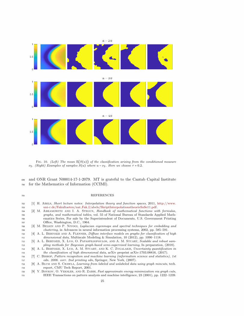
Fig. 10. (Left) The mean E(S(u)) of the classification arising from the conditioned measureν2. (Right) Examples of samples S(u) where u ∼ ν2. Here we choose τ = 0.2.
and ONR Grant N00014-17-1-2079. MT is grateful to the Cantab Capital Institute699
for the Mathematics of Information (CCIMI).700
REFERENCES701
[1] H. Abels, Short lecture notes: Interpolation theory and function spaces, 2011, http://www.702
uni-r.de/Fakultaeten/nat Fak I/abels/SkriptInterpolationstheorieSoSe11.pdf.703
[2] M. Abramowitz and I. A. Stegun, Handbook of mathematical functions with formulas,704
graphs, and mathematical tables, vol. 55 of National Bureau of Standards Applied Math-705
ematics Series, For sale by the Superintendent of Documents, U.S. Government Printing706
Office, Washington, D.C., 1964.707
[3] M. Belkin and P. Niyogi, Laplacian eigenmaps and spectral techniques for embedding and708
clustering, in Advances in neural information processing systems, 2002, pp. 585–591.709
[4] A. L. Bertozzi and A. Flenner, Diffuse interface models on graphs for classification of high710
dimensional data, Multiscale Modeling & Simulation, 10 (2012), pp. 1090–1118.711
[5] A. L. Bertozzi, X. Luo, O. Papaspiliopoulos, and A. M. Stuart, Scalable and robust sam-712
pling methods for Bayesian graph-based semi-supervised learning, In preparation, (2018).713
[6] A. L. Bertozzi, X. Luo, A. M. Stuart, and K. C. Zygalakis, Uncertainty quantification in714
the classification of high dimensional data, arXiv preprint arXiv:1703.08816, (2017).715
[7] C. Bishop, Pattern recognition and machine learning (information science and statistics), 1st716
edn. 2006. corr. 2nd printing edn, Springer, New York, (2007).717
[8] A. Blum and S. Chawla, Learning from labeled and unlabeled data using graph mincuts, tech.718
report, CMU Tech Report, 2001.719
[9] Y. Boykov, O. Veksler, and R. Zabih, Fast approximate energy minimization via graph cuts,720
IEEE Transactions on pattern analysis and machine intelligence, 23 (2001), pp. 1222–1239.721
25
[10] A. Braides, Γ-Convergence for Beginners, Oxford University Press, Oxford, 2002.722
[11] M. Burger and S. Osher, A survey on level set methods for inverse problems and optimal723
design, Europ. J. Appl. Math., 16 (2005), pp. 263–301.724
[12] J. Calder, The game theoretic p-Laplacian and semi-supervised learning with few labels, arXiv725
preprint arXiv:1711.10144, (2017).726
[13] V. Chen, M. M. Dunlop, O. Papasiliopoulos, and A. M. Stuart, Robust MCMC sampling727
with non-Gaussian and hierarchical priors in high dimensions. In Preparation.728
[14] S. L. Cotter, G. O. Roberts, A. M. Stuart, and D. White, MCMC methods for functions:729
modifying old algorithms to make them faster., Statistical Science, 28 (2013), pp. 424–446.730
[15] R. Cristoferi and M. Thorpe, Large data limit for a phase transition model with the p-731
Laplacian on point clouds, arxiv preprint arXiv:1802.08703, (2018).732
[16] G. Dal Maso, An Introduction to Γ-Convergence, Springer, 1993.733
[17] M. Dashti and A. M. Stuart, The Bayesian approach to inverse problems, in Handbook of734
Uncertainty Quantification, Springer, 2016, p. arxiv preprint arXiv:1302.6989.735
[18] M. Dunlop, C. Elliott, V. Hoang, and A. Stuart, Bayesian formulations of multidimen-736
sional barcode inversion. arXiv preprint arXiv:1706.01960.737
[19] N. Garcıa Trillos, Z. Kaplan, T. Samakhoana, and D. Sanz-Alonso, On the consistency738
of graph-based Bayesian learning and the scalability of sampling algorithms, arXiv preprint739
arXiv:1710.07702, (2017).740
[20] N. Garcıa Trillos and D. Sanz-Alonso, Continuum limit of posteriors in graph Bayesian741
inverse problems, arXiv preprint arXiv:1706.07193, (2017).742
[21] N. Garcıa Trillos and D. Slepcev, A variational approach to the consistency of spectral743
clustering, Applied and Computational Harmonic Analysis, (2016).744
[22] N. Garcıa Trillos and D. Slepcev, On the rate of convergence of empirical measures in745
∞-transportation distance, Canadian Journal of Mathematics, 67 (2015), pp. 1358–1383.746
[23] N. Garcıa Trillos and D. Slepcev, Continuum limit of total variation on point clouds,747
Archive for Rational Mechanics and Analysis, 220 (2016), pp. 193–241.748
[24] J. E. Gilbert, Interpolation between weighted Lp-spaces, Ark. Mat., 10 (1972), pp. 235–249,749
doi:10.1007/BF02384812, http://dx.doi.org/10.1007/BF02384812.750
[25] D. Grieser, Uniform bounds for eigenfunctions of the Laplacian on manifolds with bound-751
ary, Comm. Partial Differential Equations, 27 (2002), pp. 1283–1299, doi:10.1081/PDE-752
120005839, https://doi.org/10.1081/PDE-120005839.753
[26] P. Grisvard, Elliptic problems in nonsmooth domains, SIAM, 2011.754
[27] L. Hormander, The spectral function of an elliptic operator, Acta Math, 121 (1968), pp. 193–755
218.756
[28] M. A. Iglesias, Y. Lu, and A. M. Stuart, A Bayesian level set method for geometric inverse757
problems, Interfaces and Free Boundary Problems, (2015).758
[29] G. Leoni, A first course in Sobolev spaces, vol. 181 of Graduate Studies in Mathematics,759
American Mathematical Society, Providence, RI, second ed., 2017.760
[30] S. Z. Li, Markov random field modeling in computer vision, Springer Science & Business Media,761
2012.762
[31] A. Madry, Fast approximation algorithms for cut-based problems in undirected graphs, in763
Foundations of Computer Science (FOCS), 2010 51st Annual IEEE Symposium on, IEEE,764
2010, pp. 245–254.765
[32] B. Nadler, N. Srebro, and X. Zhou, Semi-supervised learning with the graph Laplacian:766
The limit of infinite unlabelled data, in Advances in neural information processing systems,767
2009, pp. 1330–1338.768
[33] R. Neal, Regression and classification using Gaussian process priors, Bayesian Statistics, 6769
(1998), p. 475. Available at http://www.cs.toronto. edu/ radford/valencia.abstract.html.770
[34] A. Y. Ng, M. I. Jordan, and Y. Weiss, On spectral clustering: Analysis and an algorithm,771
in Advances in neural information processing systems, 2002, pp. 849–856.772
[35] J. Peetre, On an interpolation theorem of Foias and Lions, Acta Sci. Math. (Szeged), 25773
(1964), pp. 255–261.774
[36] J. Shi and J. Malik, Normalized cuts and image segmentation, IEEE Transactions on pattern775
analysis and machine intelligence, 22 (2000), pp. 888–905.776
[37] Z. Shi, S. Osher, and W. Zhu, Weighted nonlocal Laplacian on interpolation from sparse777
data, Journal of Scientific Computing, 73 (2017), pp. 1164–1177.778
[38] D. Slepcev and M. Thorpe, Analysis of p-Laplacian regularization in semi-supervised learn-779
ing, arXiv preprint arXiv:1707.06213, (2017).780
[39] C. D. Sogge and S. Zelditch, Riemannian manifolds with maximal eigenfunction growth,781
Duke Math. J., 114 (2002), pp. 387–437, https://doi.org/10.1215/S0012-7094-02-11431-8.782
[40] A. Szlam and X. Bresson, Total variation and Cheeger cuts, in Proceedings of the 27th783
26
International Conference on Machine Learning, 2010, pp. 1039–1046.784
[41] M. Thorpe and A. M. Johansen, Convergence and rates for fixed-interval multiple-track785
smoothing using k-means type optimization, Electronic Journal of Statistics, 10 (2016),786
pp. 3693–3722.787
[42] M. Thorpe and F. Theil, Asymptotic analysis of the Ginzburg-Landau functional on point788
clouds, to appear in the Proceedings of the Royal Society of Edinburgh Section A: Mathe-789
matics, arXiv preprint arXiv:1604.04930, (2017).790
[43] M. Thorpe, F. Theil, A. M. Johansen, and N. Cade, Convergence of the k-means mini-791
mization problem using Γ-convergence, SIAM Journal on Applied Mathematics, 75 (2015),792
pp. 2444–2474.793
[44] Y. Van Gennip and A. L. Bertozzi, Γ-convergence of graph Ginzburg-Landau functionals,794
Advances in Differential Equations, 17 (2012), pp. 1115–1180.795
[45] U. Von Luxburg, A tutorial on spectral clustering, Statistics and computing, 17 (2007),796
pp. 395–416.797
[46] U. Von Luxburg, M. Belkin, and O. Bousquet, Consistency of spectral clustering, The798
Annals of Statistics, (2008), pp. 555–586.799
[47] G. Wahba, Spline models for observational data, SIAM, 1990.800
[48] C. K. Williams and C. E. Rasmussen, Gaussian processes for regression, in Advances in801
neural information processing systems, 1996, pp. 514–520.802
[49] D. Zhou, O. Bousquet, T. N. Lal, J. Weston, and B. Scholkopf, Learning with local and803
global consistency, in Advances in neural information processing systems, 2004, pp. 321–804
328.805
[50] X. Zhou and M. Belkin, Semi-supervised learning by higher order regularization., in AIS-806
TATS, 2011, pp. 892–900.807
[51] X. Zhu, Semi-supervised learning literature survey, tech. report, Computer Science, University808
of Wisconsin-Madison, 2005.809
[52] X. Zhu, Semi-supervised learning with graphs, PhD thesis, Carnegie Mellon University, lan-810
guage technologies institute, school of computer science, 2005.811
[53] X. Zhu, Z. Ghahramani, and J. Lafferty, Semi-supervised learning using Gaussian fields812
and harmonic functions, in Proceedings of the 20th International Conference on Machine813
Learning, vol. 3, 2003, pp. 912–919.814
[54] X. Zhu, J. D. Lafferty, and Z. Ghahramani, Semi-supervised learning: From Gaussian815
fields to Gaussian processes, tech. report, CMU Tech Report:CMU-CS-03-175, 2003.816
7. Appendix.817
7.1. Function Spaces. Here we establish the equivalence between the spectrally818
defined Sobolev spaces, Hs(Ω) and the standard Sobolev spaces.819
We denote by820
H2N(Ω) = u ∈H2(Ω) ∶ ∂u
∂n= 0 on ∂Ω
the domain of L. Analogously we denote by H2mN (Ω) the domain of Lm, that is821
H2mN (Ω) = u ∈H2m(Ω) ∶ ∂L
ru
∂n= 0 for all 0 ≤ r ≤m − 1 on ∂Ω
Finally we let H2m+1N (Ω) =H2m+1(Ω) ∩H2m
N (Ω).822
For m ≥ 0 and u, v ∈ H2m+1N (Ω) let ⟨u, v⟩2m+1,µ = ∫Ω∇Lmu ⋅ ∇Lmvρ2dx and for823
u, v ∈H2mN (Ω) let ⟨u, v⟩2m,µ = ∫Ω(Lmu)(Lmv)ρdx. We note that on the L2
µ orthogonal824
complement of the constant function 1, ⟨ ⋅ , ⋅ ⟩2m+1,µ defines an inner product, which825
due to Poincare inequality is equivalent to the standard inner product on H2m+1(Ω).826
We also note that ⟨ϕk, ϕk⟩2m+1,µ = λ2m+1k , where we recall that ϕk is unit eigenvector827
of L corresponding to λk.828
Lemma 16. Under Assumptions 2 - 3, for any integer s ≥ 0829
HsN(Ω) =Hs(Ω)
and the associated inner products ⟨ ⋅ , ⋅ ⟩s,µ and ⟪ ⋅ , ⋅⟫s,µ are equivalent on the L2µ830
orthogonal complement of the constant function.831
27
Proof. For s = 0, H0N = L2 by definition and H0 = L2 by the fact that ϕk ∶ k =832
1, . . . is an orthonormal basis.833
To show the claim for s = 1, we recall that ∫ ∇ϕk ⋅ ∇ϕjρ2dx = ∫ ϕkLϕjρdx =834
λkδjk. Therefore ϕk√
λk∶ k ≥ 1 is an orthonormal basis of the orthogonal complement835
of the constant function, 1⊥, in H1N with respect to inner product (u, v) = ∫ ∇u ⋅836
∇vρ2dx which is equivalent to the standard inner product of H1N on 1⊥. Since an837
expansion in the basis ϕkk is unique, this implies that for any u ∈ H1N = H1 the838
series ∑k akϕk converges in H1 to u. Consequently if u ∈H1N then ∞ > ∫ ∣∇u∣2ρ2dx =839
∫ ∣∑k ak∇ϕk ∣2ρ2dx = ∑k a2kλk which implies that u ∈H1. So H1
N ⊆H1.840
On the other hand, if u ∈ H1 then u = ∑k akϕk with ∑k λka2k < ∞. Therefore841
u = u +∑∞k=2 ak√λk
ϕk√λk
, where u is the average of u. Since ϕk√λk
are orthonormal in842
scalar product with topology equivalent to H1, the series converges in H1. Therefore843
u ∈H1 =H1N .844
Assume now that the claim holds for all integers less than s. We split the proof845
of the induction step into two cases:846
Case 1 Consider s even; that is s = 2m for some integer m > 0.847
Assume u ∈ H2mN . Then ∇Lru ⋅ n = 0 on ∂Ω for all r < m. By the induction848
hypothesis ∑k λ2m−1k a2
k < ∞. Since L is a continuous operator from H2 to L2 one849
obtains by induction that Lm−1u = ∑k akLm−1ϕk = ∑akλm−1k ϕk. Let v = Lm−1u. By850
assumption v ∈H2N . By above v = ∑k akλm−1
k ϕk.851
Since ϕk is solution of Lϕk = λkϕk852
⟨Lϕk, v⟩µ = ⟨λkϕk, v⟩µ.
Using that v ∈H2, ∇v ⋅ n = 0 on ∂Ω and integration by parts we obtain853
⟨ϕk,Lv⟩µ = ⟨λkϕk,∑j
ajλm−1j ϕj⟩µ = λmk ak.
Given that Lv is an L2µ function, we conclude that Lv = ∑k λmk akϕk. Therefore854
∑k λ2mk a2
k <∞ and hence u ∈H2m.855
To show the opposite inclusion, consider u ∈ H2m. Then u = ∑k akϕk and
∑k λ2mk a2
k <∞. By induction step we know that u ∈ H2m−2N and thus v = Lm−1u ∈ L2.
We conclude as before that v = ∑k λm−1k akϕk. Let bk = λm−1
k ak. Assumptions on uimply ∑k λ2
kb2k < ∞. Arguing as above in the case s = 1 we conclude that the se-
ries converges in H1 and that ∇v = ∑k bk∇ϕk. Combining this with the fact thatLϕk = λkϕk in Ω for all k implies that v is a weak solution of
Lv =∑k
λkbkϕk in Ω,
∂v
∂n= 0 on ∂Ω.
Since RHS of the equation is in L2 and ∂Ω is C1,1, by elliptic regularity [26], v ∈H2 and856
∥v∥2H2 ≤ C(Ω, ρ)∑k b2kλ2
k. Furthermore v satisfies the Neumann boundary condition857
and thus v ∈H2N .858
Case 2 Consider s odd; that is s = 2m + 1 for some integer m > 0. Assume859
u ∈ H2m+1N . Let v = Lmu. Then v ∈ H1. The result now follows analogously to the860
case s = 1. If u ∈ H2m+1 then, u = ∑k akϕk with ∑k λ2m+1k a2
k < ∞. By induction861
hypothesis, v = Lm−1u ∈ H1N and v = ∑k bkϕk where bk = λm−1ak. Thus ∑k λkb2k <∞862
and the argument proceeds as in the case s = 1.863
28
Proving the equivalence of inner products is straightforward.864
We now present the proof of Lemma 3.865
Proof of Lemma 3. If s is integer the claim follows form Lemma 16 and Sobolev866
embedding theorem. Assume s = m + θ for some θ ∈ (0,1). Since Ω is Lipschitz,867
by extension theorem of Stein (Leoni [29] 2nd edition, Theorem 13.17) there is a868
bounded linear extension mapping Em ∶ Hm(Ω) → Hm(Rd) such that Em(f)∣Ω = f .869
From the construction (see remark 13.9 in [29]) it follows that Em and Em+1 agree870
on smooth functions and thus Em+1 = Em∣Hm(Ω). Therefore, by Theorem 16.12 in871
Leoni’s book (or Lemma 3.7 of Abels [1]) Em provides a bounded mapping from the872
interpolation space [Hm(Ω),Hm+1(Ω)]θ,2 → [Hm(Rd),Hm+1(Rd)]θ,2. As discussed873
above the statement of Lemma 3 Hm+θ(Ω) = [Hm(Ω),Hm+1(Ω)]θ,2. By Lemma874
16, [Hm(Ω),Hm+1(Ω)]θ,2 embeds into [Hm(Ω),Hm+1(Ω)]θ,2. Furthermore, we use875
that, see Abels [1] Corollary 4.15, [Hm(Rd),Hm+1(Rd)]θ,2 = Hm+θ(Rd). Combining876
these facts yields the existence of an bounded, linear, extension mapping Hm+θ(Ω)→877
Hm+θ(Rd). The results (i) and (ii) follows by the Sobolev embedding theorem.878
7.2. Passage from Discrete to Continuum. There are two key tools we879
use to pass from the discrete to continuum limit. The first is Γ-convergence. Γ-880
convergence was introduced in the 1970’s by De Giorgi as a tool for studying sequences881
of variational problems. More recently this methodology has been applied to study882
the large data limits of variational problems that arise from statistical inference,883
e.g. [21, 23, 41, 42, 43]. Accessible introductions to Γ-convergence can be found884
in [10, 16]885
The Γ-convergence methodology provides a notion of convergence of functionals886
that captures the behaviour of minimizers. In particular the minimizers converge887
along a subsequence to a minimizer of the limiting functional. In our setting, the888
objects of interest are functions on discrete domains and hence it is not immediate889
how one should define convergence. This brings us to our second key tool. Recently890
a suitable topology has been identified to characterize the convergence of discrete to891
continuum using an optimal transport framework [23]. The main idea is, given a892
discrete function un ∶ Ωn → R and a continuum function u ∶ Ω → R, to include the893
measures with respect to which they are defined in the comparison. Namely, one can894
think of the function un as belonging to the Lp space over the empirical measure895
µn = 1n ∑
ni=1 δxi and u belonging to the Lp space over the measure µ. One defines896
a continuum function un ∶ Ω → R by un = un Tn where Tn ∶ Ωn → Ω is a measure897
preserving map between µ and µn. One then compares un and un in the Lp distance,898
and simultaneously compares Tn and identity. In other words one considers both the899
difference in values and the how far the matched points are. We give a brief overview900
of Γ-convergence and the TLp space.901
7.2.1. A Brief Introduction to Γ-Convergence. We present the definition902
of Γ-convergence in terms of an abstract topology. In the next section we will discuss903
what topology we will use in our results. For now, we simply point out that the space904
X needs to be general enough to include functions defined with respect to different905
measures.906
Definition 17. Given a topological space X , we say that a sequence of func-907
tions Fn ∶ X → R ∪ +∞ Γ-converges to F∞ ∶ X → R ∪ +∞, and we write908
F∞ = Γ- limn→∞ Fn, if the following two conditions hold:909
29
(the liminf inequality) for any convergent sequence un → u in X910
lim infn→∞
Fn(un) ≥ F∞(u);
(the limsup inequality) for every u ∈ X there exists a sequence un in X with911
un → u and912
lim supn→∞
Fn(un) ≤ F∞(u).
In the above definition we also call any sequence unn=1,... that satisfies the lim-913
sup inequality a recovery sequence. The justification of Γ-convergence as the natural914
setting to study sequences of variational problems is given by the next proposition.915
The proof can be found in, for example, [10].916
Proposition 18. Let Fn, F∞ ∶ X → R∪ +∞. Assume that F∞ is the Γ-limit of917
Fn and the sequence of minimizers unn=1,... of Fn is precompact. Then918
limn→∞
minX
Fn = limn→∞
Fn(un) = minX
F∞
and furthermore, any cluster point u of unn=1,... is a minimizer of F∞.919
Note that Γ- limn→∞ Fn = F∞ and Γ- limn→∞Gn = G∞ does not imply Fn +Gn Γ-920
converges to G∞+F∞. Hence, in order to build optimization problems by considering921
individual terms it is not enough, in general, to know that each term Γ-converges. In922
particular, we consider using the quadratic form J(α,τ)n as a prior and adding fidelity923
terms, e.g.924
J(n)(u) = J(α,τ)n (u) +Φ(n)(u).
We show that, with probability one, Γ- limn→∞ J(α,τ)n = J
(α,τ)∞ . In order to show925
that J(n) Γ-converges it suffices to show that Φ(n) converges along any sequence926
(µn, un) along which J(α,τ)n (un) is finite. This is similar to the notion of continuous927
convergence, which is typically used [16, Proposition 6.20]. However we note that928
Φ(n) does not converge continuously since as a functional on TLp(Ω) it takes the929
value infinity whenever the measure considered is not µn.930
7.2.2. The TLp Space. In this section we give an overview of the topology that931
was introduced in [23] to compare sequences of functions on graphs. We motivate the932
topology in the setting considered in this paper. Recall that µ ∈ P(Ω) has density ρ933
and that µn is the empirical measure. Given un ∶ Ωn → R and u ∶ Ω→ R the idea is to934
consider pairs (µ,u) and (µn, un) and compare them as such. We define the metric935
as follows.936
Definition 19. Given a bounded open set Ω, the space TLp(Ω) is the space of937
pairs (µ, f) such that µ is a probability measure supported on Ω and f ∈ Lp(µ). The938
metric on TLp is defined by939
dTLp((f, µ), (g, ν)) = infπ∈Π(µ,ν)
(∫Ω×Ω
∣x − y∣p + ∣f(x) − g(y)∣p dπ(x, y))1p
.
Above Π(µ, ν) is the set of transportation plans (i.e. couplings) between µ and ν;940
that is the set of probability measures on Ω ×Ω whose first marginal is µ and second941
marginal in ν.942
For a proof that dTLp is a metric on TLp see [23, Remark 3.4].943
30
To connect the TLp metric defined above with the ideas discussed previously we944
make several observations. The first is that when µ has a continuous density then one945
can consider transport maps T ∶ Ω → Ωn that satisfy T#µ = µn instead of transport946
plans π ∈ Π(µ, ν). Hence, one can show that947
dTLp((f, µ), (g, ν)) = infT ∶T#µ=ν
(∥Id − T ∥pLp(µ) + ∥f − g T ∥p
Lp(µ))1p.
In the setting when we compare (µ,u) and (µn, un) the second term is nothing948
but ∥u − un∥pLp(µ), where un = un Tn and Tn ∶ Ω→ Ωn is a transport map.949
We note that for a sequence (µn, un) to TLp converge to (µ,u) it is necessary950
that ∥Id−T ∥Lp(µ) converges to zero, in other words it is necessary that the measures951
µn converge to µ in p-optimal transportation distance. We recall that since Ω is952
bounded this is equivalent to weak convergence of µn to µ. Assuming this to be the953
case, we call any sequence of transportation maps Tn satisfying (Tn)#µ = µn and954
∥Id − Tn∥Lp(µ) → 0 a stagnating sequence. One can then show (see [23, Proposition955
3.12]) that convergence in TLp is equivalent to weak* convergence of measures µn956
to µ and convergence ∥u − un Tn∥Lp(µ) → 0 for arbitrary sequence of stagnating957
transportation maps. Furthermore if convergence ∥u − un Tn∥Lp(µ) → 0 holds for a958
sequence of stagnating transportation maps it holds for every sequence of stagnating959
transportation maps.960
The intrinsic scaling of the graph Laplacian, i.e. the parameter εn, depends on961
how far one needs to move “mass” to couple µ and µn, that is on upper bounds on962
transportation distance between µ and µn. The following result can be found in [22],963
the lower bound in the scaling of ε = εn is so that there exists a stagnating sequence964
of transport maps with ∥Tn−Id∥L∞εn
→ 0.965
Proposition 20. Let Ω ⊂ Rd with d ≥ 2 be open, connected and bounded with966
Lipschitz boundary. Let µ ∈ P(Ω) with density ρ which is bounded above and below by967
strictly positive constants. Let Ωn = xini=1 where xiiid∼ µ and let µn = 1
n ∑ni=1 δxi be968
the associated empirical measure. Then, there exists C > 0 such that, with probability969
one, there exists a sequence of transportation maps Tn ∶ Ω → Ωn that pushes µ onto970
µn and such that971
lim supn→∞
∥Tn − Id∥L∞(Ω)δn
≤ C
where972
δn =⎧⎪⎪⎪⎨⎪⎪⎪⎩
(logn)34√
nif d = 2
( lognn
)1d if d ≥ 3.
7.3. Estimates on Eigenvalues of the Graph Laplacian. The following973
lemma is nonasymptotic and holds for all n. However we will use it in the asymptotic974
regime and note that our assumptions on ε, (5), and results of Proposition 20 ensure975
that the assumptions of the lemma are satisfied.976
Lemma 21. Consider the operator A(n) defined in (1) for α = 1 and τ ≥ 0. As-977
sume that dOT∞(µn, µ) < ε. Then the spectral radius λmax of A(n) is bounded by978
C 1ε2+ τ2 where C > 0 is independent of n and ε.979
Let R > 0 be such that η(3R) > 0. Assume that dOT∞(µn, µ) < Rε. Then there980
exists c > 0, independent of n and ε, such that λmax > c 1ε2+ τ2.981
31
Proof. Let η(x) = η((∣x∣−1)+). Note that η ≥ η(∣ ⋅ ∣) and that since η is decreasing982
and integrable ∫Rd η(x)dx <∞.983
Let T be the dOT∞ transport map from µ to µn. By assumption ∥Tn(x) − x∥ ≤ ε984
a.e. By definition of A(n)985
λmax = sup∥u∥L2
µn=1
⟨u,A(n)u⟩µn = τ2 + sup∥u∥L2
µn=1
⟨u, snLu⟩µn
We estimate
sup∥u∥L2
µn=1
⟨u, snLu⟩µn ≤ sup1n ∑ni=1 u2
i=1
4
ση∑i,j
1
n2εd+2η ( ∣xi − xj ∣
ε)(u2
i + u2j)
≲ sup1n ∑ni=1 u2
i=1
n
∑i=1
n
∑j=1
1
n2εd+2η ( ∣xi − xj ∣
ε)u2
i
= sup1n ∑ni=1 u2
i=1
1
nεd+2
n
∑i=1
u2i ∫
Ωη ( ∣xi − T (x)∣
ε)dµ(x)
≤ sup1n ∑ni=1 u2
i=1
1
nεd+2
n
∑i=1
u2i ∫
Ωη (xi − x
ε)dµ(x)
≲ 1
ε2 ∫Rd η(z)dz ≲1
ε2.
Above ≲ means ≤ up to a factor independent of ε and n.986
To prove the second claim of the lemma consider v = √nδxi , a singleton concen-
trated at an arbitrary xi, that is vi =√n and vj = 0 for all j ≠ i. Then ∥v∥L2
µn= 1.
Using that for a.e. x ∈ B(xi,2εR), ∣xi − T (x)∣ ≤ 3εR we estimate:
sup∥u∥L2
µn=1
⟨u, snLu⟩µn ≥ ⟨v, snLv⟩µn
≳∑j≠i
n
n2εd+2η ( ∣xi − xj ∣
ε)
= 1
εd+2 ∫Ω∖T−1(xi)η ( ∣xi − T (x)∣
ε)dµ(x)
≥ 1
εd+2 ∫B(xi,2εR)∖B(xi,εR)η(3R)dµ(x) ≳ 1
ε2(25)
which implies the claim.987
An immediate corollary of the claim is the characterization of the energy of a988
singleton. For any α ≥ 1 and τ ≥ 0.989
(26) J(α,τ)n (δxi) ∼1
n( 1
ε2n
+ τ2)α
∼ 1
nε2αn
.
The upper bound is immediate from the first part of the lemma, while the lower bound990
follows from the second part of the lemma via Jensen’s inequality. Namely, (λ(n)k , q(n)k )991
be eigenpairs of L and let us expand δxi in the terms of q(n)k : i.e. δxi = ∑nk=1 akq
(n)k992
where ∑k a2k = ∥δxi∥2
L2µn
= 1n
. We know that ∑k λ(n)k a2
k ≳ 1nε2nsn
∼ 1, from (25) (using993
32
the expansion (27) and noting that v = √nδxi in (25)). Hence994
J(α,τ)n (δxi) =1
2n
n
∑k=1
(snλ(n)k + τ2)αna2
k ≥1
2n(nsn
n
∑k=1
λ(n)k a2
k + τ2)α
≥ 1
2n( 1
ε2n
+ τ2)α
.
995
7.4. The Limiting Quadratic Form. Here we prove Theorem 1. The key tool996
is to use spectral decomposition of the relevant quadratic forms, and to rely on the997
limiting properties of the eigenvalues and eigenvectors of L established in [21].998
Let (q(n)k , λ(n)k ) be eigenpairs of L with eigenvalues λk ordered so that999
0 = λ(n)1 ≤ λ(n)2 ≤ λ(n)3 ≤ . . . λ(n)n
where λ(n)1 < λ(n)2 provided that the graph G is connected. We extend F ∶ R ↦ R to1000
a matrix-valued function F via F (L) = Q(n)(Λ(n)F )(Q(n))∗ where Q(n) is the matrix1001
with columns q(n)k nk=1 and Λ(n)F is the diagonal matrix with entries F (λ(n)i )ni=1.1002
For constants α ≥ 1, τ ≥ 0 and a scaling factor sn, given by (6), we recall the definition1003
of the precision matrix A(n) is A(n) = (snL+ τ2I)α and the fractional Sobolev energy1004
J(α,τ)n is1005
J(α,τ)n ∶ L2µn ↦ [0,+∞), J(α,τ)n (u) = 1
2⟨u,A(n)u⟩µn .
Note that1006
(27) J(α,τ)n (u) = 1
2
n
∑k=1
(snλ(n)k + τ2)α⟨u, q(n)k ⟩2µn .
When showing Γ-convergence, all functionals are considered as functionals on the TLp1007
space. When evaluating J(α,τ)n at (ν, u) we consider it infinite for any measure ν other1008
than µn, and having the value J(α,τ)n (u) defined above if ν = µn.1009
We let (qk, λk) for k = 1,2, . . . be eigenpairs of L ordered so that1010
0 = λ1 ≤ λ2 ≤ λ3 ≤ . . . .
We extend F ∶ R ↦ R to an operator valued function via the identity F (L) =1011
∑∞k=1 F (λk)⟨u, qk⟩µqk. For constants α ≥ 1 and τ ≥ 0 we recall the definition of1012
the precision operator A as A = (L + τI)α and the continuum Sobolev energy J(α,τ)∞1013
as1014
J(α,τ)∞ ∶ L2µ ↦ R ∪ +∞, J(α,τ)∞ (u) = 1
2⟨u,Au⟩µ.
Note that the Sobolev energy can be written1015
J(α,τ)∞ (u) = 1
2
∞∑k=1
(λk + τ2)α⟨u, qk⟩2µ.
Proof of Theorem 1. We prove the theorem in three parts. In the first part we1016
prove the liminf inequality and in the second part the limsup inequality. The third1017
part is devoted to the proof of the two compactness results.1018
33
The Liminf Inequality. Let un → u in TLp, we wish to show that1019
lim infn→∞
J(α,τ)n (un) ≥ J(α,τ)∞ (u).
By [21, Theorem 1.2], if all eigenvalues of L are simple, we have with probability one1020
(where the set of probability one can be chosen independently of the sequence un1021
and u) that snλ(n)k → λk and q
(n)k converge in TL2 to qk. If there are eigenspaces1022
of L of dimension higher than one then q(n)k converge along a subsequence in TL2
1023
to eigenfunctions qk corresponding to the same eigenvalue as qk. In this case we1024
replace qk by qk, which does not change any of the functionals considered. We note1025
that while eigenvectors in the general case only converge along subsequences, the1026
projections to the relevant spaces of eigenvectors converge along the whole sequence,1027
see [21, statement 3. Theorem 1.2]. To prove the convergence of the functional one1028
would need to use these projections, which makes the proof cumbersome. For that1029
reason in the remainder of the proof we assume that all eigenvalues of L are simple, in1030
which case we can express the projections using the inner product with eigenfunctions.1031
Since q(n)k → qk and un → u in TL2 as n→∞, ⟨q(n)k , un⟩µn → ⟨q, u⟩µ as n→∞.1032
First we assume that J(α,τ)∞ (u) <∞. Let δ > 0 and choose K such that1033
1
2
K
∑k=1
(λk + τ2)α⟨u, qk⟩2µ ≥ J(α,τ)∞ (u) − δ.
Now,
lim infn→∞
J(α,τ)n (un) ≥ lim infn→∞
1
2
K
∑k=1
(snλ(n)k + τ2)α⟨un, q(n)k ⟩2µn
= 1
2
K
∑k=1
(λk + τ2)α⟨un, qk⟩2µ
≥ J(α,τ)∞ (u) − δ.
Let δ → 0 to complete the liminf inequality for when J(α,τ)∞ (u) <∞. If J
(α,τ)∞ (u) = +∞1034
then choose any M > 0 and find K such that 12 ∑
Kk=1(λk+τ2)α⟨un, qk⟩2µ ≥M , the same1035
argument as above implies that1036
lim infn→∞
J(α,τ)n (un) ≥M
and therefore lim infn→∞ J(α,τ)n (un) = +∞.1037
The Limsup Inequality. As above, we assume for simplicity, that all eigenvalues1038
of L are simple. We remark that there are no essential difficulties to carry out the1039
proof in the general case.1040
Let u ∈ L2µ with J
(α,τ)∞ (u) <∞ (the proof is trivial if J
(α,τ)∞ =∞). Define un ∈ L2
µn1041
by un = ∑Knk=1 ψkq(n)k where ψk = ⟨u, qk⟩µ. Let Tn be the transport maps from µ to µn1042
as in Proposition 20. Let ank = ψkq(n)k Tn and ak = ψkqk. By Lemma 24, there exists1043
a sequence Kn →∞ such that un converges to u in TL2 metric.1044
We recall from the proof of the liminf inequality that ⟨q(n)k , un⟩µn → ⟨qk, u⟩µ as1045
n→∞. Combining with the convergence of eigenvalues, [21, Theorem 1.2], implies1046
(snλ(n)k + τ2)α⟨un, q(n)k ⟩2µn → (λk + τ2)α⟨u, qk⟩2µ34
as n → ∞. Taking ank = (snλ(n)k + τ2)α⟨un, q(n)k ⟩2µn and ak = (λk + τ2)α⟨u, qk⟩2µ and1047
using Lemma 24 implies that there exists Kn ≤ Kn converging to infinity such that1048
∑Knk=1 ank → ∑
∞k=1 ak as n → ∞. Let un = ∑Knk=1 ψkq
(n)k . Then un → u in TL2. Further-1049
more J(α,τ)n (un) = ∑Knk=1 a
nk and J
(α,τ)∞ (u) = ∑∞k=1 ak which implies that J
(α,τ)n (un) →1050
J(α,τ)∞ (u) as n→∞.1051
Compactness. If τ > 0 and supn∈N J(α,τ)n (un) ≤ C then1052
τ2α∥un∥2L2µn
= τ2αn
∑k=1
⟨un, q(n)k ⟩2µn ≤n
∑k=1
(snλ(n)k + τ2)α⟨un, q(n)k ⟩2µn ≤ C.
Therefore ∥un∥L2µn
is bounded. Hence in statements 2 and 3 of the theorem we have1053
that ∥un∥L2µn
and J(α,τ)n (un) are bounded. That is there exists C > 0 such that1054
(28) ∥u∥2L2µn
=n
∑k=1
⟨un, q(n)k ⟩µn ≤ C and sαn
n
∑k=1
(λ(n)k )α⟨un, q(n)k ⟩2µn ≤ C.
We will show there exists u ∈ L2µ and a subsequence nm such that unm converges to u1055
in TL2.1056
Let ψnk = ⟨un, q(n)k ⟩µn for all k ≤ n. Due to (28) ∣ψnk ∣ are uniformly bounded.1057
Therefore, by a diagonal procedure, there exists a increasing sequence nm →∞ as m→1058
∞ such that for every k, ψnmk converges as m→∞. Let ψk = limm→∞ ψnmk . By Fatou’s1059
lemma, ∑∞k=1 ∣ψk ∣2 ≤ lim infm→∞∑nmk=1 ∣ψnmk ∣2 ≤ C. Therefore u ∶= ∑∞k=1 ψkqk ∈ L2µ.1060
Using Lemma 24 and arguing as in the proof of the limsup inequality we obtain that1061
there exists a sequence Km increasing to infinity such that ∑Kmk=1 ψnmk q
(nm)k converges1062
to u in TL2 metric as m→∞. To show that unm converges to u in TL2, we now only1063
need to show that ∥unm −∑Kmk=1 ψnmk q
(nm)k ∥L2
µnmconverges to zero. This follows from1064
the fact that1065
nm
∑k=Km+1
∣ψnmk ∣2 ≤ 1
(λ(nm)Km)α
nm
∑k=Km+1
(λ(nm)k )α∣ψnmk ∣2 ≤ C
(snmλ(nm)Km
)α
using that the sequence of eigenvalues is nondecreasing. Now since snmλ(nm)Km
≥1066
snmλ(nm)K → λK for all Km ≥K, and limK→∞ λK = +∞ we have that snmλ
(nm)Km
→ +∞1067
as m→∞, hence unm converges to u in TL2.1068
Remark 22. Note that when α ≥ 1 the compactness property holds trivially from1069
the compactness property for α = 1, see [21, Theorem 1.4], as J(α,τ)n (un) ≥ J(1,0)n (un).1070
7.5. Variational Convergence of Probit in Labelling Model 1. To prove1071
minimizers of the Probit model in Labelling Model 1 converge we apply Proposi-1072
tion 18. This requires us to show that J(n)p Γ-converges to J
(∞)p and the compactness1073
of sequences of minimizers. Recall that J(n)p = J(α,τ)n + 1
nΦ(n)p (⋅;γ). Hence Theorem 11074
establishes the Γ-convergence of the first term. We now show that 1n
Φ(n)p (un; yn;γ)→1075
Φp,1(u; y;γ) whenever (µn, un) → (µ,u) in the TL2 sense, which is enough to es-1076
tablish Γ-convergence. Namely since, by definition, J(α,τ)n applied to an element1077
(ν, v) ∈ TLp(Ω) is ∞ if ν ≠ µn it suffices to consider sequences of the form (µn, un)1078
to show the liminf inequality. The limsup inequality is also straightforward since the1079
the recovery sequence for J(α,τ)∞ is also of the form (µn, un).1080
35
Lemma 23. Consider domain Ω and measure µ satisfying Assumptions 2–3. Let1081
xiiid∼ µ for i = 1, . . . , n, Ωn = x1, . . . , xn and µn be the empirical measure of the1082
sample. Let Ω′ be an open subset of Ω, µ′n = µn⌊Ω′ and µ′ = µ⌊Ω. Let yn ∈ L∞(µ′n) and1083
y ∈ L∞(µ′) and let yn ∈ L∞(µn) and y ∈ L∞(µ) be their extensions by zero. Assume1084
(µn, yn)→ (µ, y) in TL∞ as n→∞.
Let Φ(n)p and Φp,1 be defined by (9) and (16) respectively, where Z ′ = j ∶ xj ∈ Ω′1085
and γ > 0 (and where we explicitly include the dependence of yn and y in Φ(n)p and1086
Φp,1).1087
Then, with probability one, if (µn, un)→ (µ,u) in TLp then1088
1
nΦ(n)p (un; yn;γ)→ Φp,1(u; y;γ) as n→∞.
Proof. Let (µn, un)→ (µ,u) in TLp. We first note that since Ψ(uy;γ) = Ψ (uyγ
; 1)and since multiplying all functions by a constant does not affect the TLp convergence,it suffices to consider γ = 1. For brevity, we omit γ in the functionals that follow. Wehave that yn Tn → y and un Tn → u. Recall that
1
nΦ(n)p (un; yn) = ∫
T−1n (Ω′
n)log Ψ(yn(Tn(x))un(Tn(x)))dµ(x)
Φp,1(u; y) = ∫Ω′
log Ψ(y(x)u(x))dµ(x),
where Ω′n = xi ∶ xi ∈ Ω′, for i = 1, . . . , n. Recall also that symmetric difference of
sets is denoted by AB = (A ∖B) ∪ (B ∖A). It follows that
∣ 1n
Φ(n)p (un; yn) −Φp,1(u; y)∣ ≤ ∣∫Ω′T−1n (Ω′
n)log Ψ(y(x)u(x))dµ(x)∣
+ ∣∫T−1n (Ω′
n)log (Ψ(yn(Tn(x))un(Tn(x));γ) − log (y(x)u(x)) dµ(x)∣ .
(29)
Define1089
∂εnΩ′ = x ∶ dist(x, ∂Ω′) ≤ εn .Then Ω′ T −1
n (Ω′n) ⊆ ∂εnΩ′. Since y ∈ L∞ and u ∈ L2
µ then yu ∈ L2µ and so by1090
Corollary 26 log Ψ(yu) ∈ L1. Hence, by the dominated convergence theorem1091
∣∫Ω′T−1n (Ω′
n)log Ψ(y(x)u(x))dµ(x)∣ ≤ ∫
∂εnΩ′
∣log Ψ(y(x)u(x))∣ dµ(x)→ 0.
We are left to show that the second term on the right hand side of (29) convergesto 0. Let F (w, v) = ∣ log Ψ(w) − log Ψ(v)∣. Let M ≥ 1 and define the following sets
An,M = x ∈ T −1n (Ω′
n) ∶ miny(x)u(x), yn(Tn(x))un(Tn(x)) ≥ −MBn,M = x ∈ T −1
n (Ω′n) ∶ y(x)u(x) ≥ yn(Tn(x))un(Tn(x)) ≤ −M
Cn,M = x ∈ T −1n (Ω′
n) ∶ yn(Tn(x))un(Tn(x)) ≥ y(x)u(x) ≤ −M .The quantity we want to estimate satisfies
∣∫T−1n (Ω′
n)log (Ψ(yn(Tn(x))un(Tn(x))) − log Ψ (y(x)u(x)) dµ(x)∣
≤ ∫T−1n (Ω′
n)F (yn(Tn(x))un(Tn(x)), y(x)u(x))dµ(x).
36
Since T −1n (Ω′
n) = An,M ∪Bn,M ∪Cn,M we proceed by estimating the integral over each1092
of the sets, utilizing the bounds in Lemma 25.1093
∫An,MF (yn(Tn(x))un(Tn(x)), y(x)u(x))dµ(x)
≤ 1
∫−M−∞ e−
t2
2 dt∫An,M
∣yn(Tn(x))un(Tn(x)) − y(x)u(x)∣ dµ(x)
≤ 1
∫−M−∞ e−
t2
2 dt(∥yn∥L2
µn∥un Tn − u∥L2
µ+ ∥u∥L2
µ∥yn Tn − y∥L2
µ) .
∫Bn,MF (yn(Tn(x))un(Tn(x)), y(x)u(x))dµ(x)
≤ ∫Bn,M2∣yn(Tn(x))∣2∣un(Tn(x))∣2 dµ(x) + 1
M2
≤ 2∥yn∥2L∞µn ∫Bn,M
∣un(Tn(x))∣2 dµ(x) + 1
M2
≤ 4∥yn∥2L∞µn
(∥un Tn − u∥2L2µ+ ∫
Ω∣u(x)∣2I∣yn(Tn(x))un(Tn(x))∣≥M dµ(x)) + 1
M2.
∫Cn,MF (yn(Tn(x))un(Tn(x)), y(x)u(x))dµ(x)
≤ ∫Cn,M2∣y(x)∣2∣u(x)∣2 dµ(x) + 1
M2
≤ 2∥y∥2L∞µ ∫Ω
∣u(x)∣2I∣y(x)u(x)∣≥M dµ(x) + 1
M2.
For every subsequence there exists a further subsequence such that (yn Tn)(un 1094
Tn)→ yu pointwise a.e., hence by the dominated convergence theorem1095
∫Ω∣u(x)∣2I∣yn(Tn(x))un(Tn(x))∣≥M dµ(x)→ ∫
Ω∣u(x)∣2I∣y(x)u(x)∣≥M dµ(x) as n→∞.
Hence, for M ≥ 1 fixed we have
lim supn→∞
∣∫T−1n (Ω′
n)log (Ψ(yn(Tn(x))un(Tn(x));γ) − log (y(x)u(x);γ) dµ(x)∣
≤ 2
M2+ 6∥y∥L∞µ ∫
Ω∣u(x)∣2I∣y(x)u(x)∣≥M dµ(x).
Taking M →∞ completes the proof.1096
The proof of Theorem 10 is now just a special case of the above lemma and an1097
easy compactness result that follows from Theorem 1.1098
Proof of Theorem 10. The following statements all hold with probability one. Let1099
y(x) = 1 if x ∈ Ω+
−1 if x ∈ Ω−.
37
Since dist(Ω+,Ω−) > 0 there exists a minimal Lipschitz extension y ∈ L∞ of y to Ω.Let yn = y⌊Ωn and yn = y⌊Ωn . Since
∥yn Tn − y∥L∞(µ) = µ-ess supx∈Ω
∣yn(Tn(x)) − y(x)∣
= µ-ess supx∈Ω
∣y(Tn(x)) − y(x)∣
≤ Lip(y)∥Tn − Id∥L∞
we conclude that (µn, yn) → (µ, y) in TL∞. Hence, by Lemma 23, 1n
Φ(n)p (un;γ) →1100
Φp,1(u;γ) whenever (µn, un) → (µ,u) in TLp. Combining with Theorem 1 implies1101
that J(n)p Γ-converges to J
(∞)p via a straightforward argument.1102
If τ > 0 then the compactness of minimizers follows from Theorem 1 using that1103
supn∈N minvn∈L2µn
J(n)p (vn) ≤ supn∈N J
(n)p (0) = 1
2.1104
When τ = 0 we consider the sequence wn = vn− vn where vn is a minimizer of J(n)p1105
and vn = ⟨vn, q1⟩µn = ∫Ω vn(x)dµn(x). Then, J(α,0)n (wn) = J(α,0)n (vn) and1106
∥wn∥2L2µn
= ∥vn − vn∥2L2µn
=n
∑k=2
⟨vn, qk⟩2µn ≤1
(snλ(n)2 )αJ(α,0)n (vn).
As in the case τ > 0 the quadratic form is bounded, i.e. supn∈N J(n)p (vn) ≤ 1
2. Hence1107
J(α,τ)n (wn) ≤ 1
2and ∥wn∥2
L2µn
≤ 1λα2
for n large enough. By Theorem 1 wn is precompact1108
in TL2. Therefore supn∈N ∥vn∥L2µn
≤ M + supn∈N ∣vn∣ for some M > 0. Since J(α,τ)n is1109
insensitive to the addition of a constant, and −1 ≤ y ≤ 1, then for any minimiser vn1110
one must have vn ∈ [−1,1]. Hence supn∈N ∥vn∥L2µn
≤ M + 1 so by Theorem 1 vn is1111
precompact in TL2.1112
Since the minimizers of J(∞)p are unique (due to convexity, see Lemma 9), by1113
Proposition 18 we have that the sequence of minimizers vn of J(n)p converges to the1114
minimizer of J(∞)p .1115
7.6. Variational Convergence of Probit in Labelling Model 2.1116
Proof of Theorem 11. It suffices to show that J(n)p Γ-converges in TL2 to J
(α,τ)∞1117
and that the sequence of minimizers vn of J(n)p is precompact in TL2. We note that1118
the liminf statement of the Γ-convergence follows immediately from statement 1. of1119
Theorem 1.1120
To complete the proof of Γ-convergence it suffices to construct a recovery sequence.1121
The strategy is analogous to the one of the proof on Theorem 4.9 of [38]. Let v ∈1122
Hα(Ω). Since J(α,τ)n Γ-converges to J
(α,τ)∞ by Theorem 1 there exists Let v(n) ∈ L2
µn1123
such that J(α,τ)n (v(n))→ J
(α,τ)∞ (v) as n→∞. Consider the functions1124
v(n)(xi) =⎧⎪⎪⎨⎪⎪⎩
cny(xi) if i = 1, . . . ,N.
v(n)(xi) if i = N + 1, . . . , n
where cn →∞ and cnε2αn n
→ 0 as n→∞.1125
Note that condition (5) implies that when α < d2
then (20) still holds. There-1126
fore (26) implies that J(α,τ)n (cnδxi) → 0 as n → ∞. Also note that since cn → ∞,1127
Φ(n)p (v(n);γ)→ 0 as n→∞. It is now straightforward to show, using the form of the1128
38
functional, the estimate on the energy of a singleton and the fact that εnn12α →∞ as1129
n→∞, that J(n)p (v(n))→ J
(α,τ)∞ (v) as desired.1130
The precompactness of vnn∈N follows from Theorem 1. Since 0 is the unique1131
minimizer of J(α,τ)∞ , due to τ > 0, the above results imply that v(n) converge to 0.1132
7.7. Small Noise Limits.1133
Proof of Theorem 14. First observe that since Assumptions 2–3 hold and α > d/2,1134
the measure ν0, and hence the measures νp,1, νp,2, ν1, are all well-defined measures on1135
L2(Ω) by Theorem 4.1136
(i) For any continuous bounded function g ∶ C(Ω;R)→ R we have
Eνp,1g(u) = Eν0e−Φp,1(u;γ)g(u)Eν0e−Φp,1(u;γ) , Eν1g(u) =
Eν01B∞,1(u)g(u)Eν01B∞,1(u)
.
For the first convergence it thus suffices to prove that, as γ → 0,
Eν0e−Φp,1(u;γ)g(u)→ Eν01B∞,1(u)g(u)
for all continuous functions g ∶ C(Ω;R)→ [−1,1].1137
We first define the standard normal cumulative distribution function ϕ(z) =1138
Ψ(z,1), and note that we may write1139
Φp,1(u;γ) = −∫x∈Ω′
log(ϕ(y(x)u(x)/γ))dx ≥ 0.
In what follows it will be helpful to recall the following standard Mills ratiobound: for all t > 0,
ϕ(t) ≥ 1 − e−t2/2
t√
2π.(30)
Suppose first that u ∈ B∞,1, then y(x)u(x)/γ > 0 for a.e. x ∈ Ω′. The1140
assumption that Ω+ ∩ Ω− = ∅ ensures that y is continuous on Ω′ = Ω+ ∪ Ω−.1141
As u is also continuous on Ω′, given any ε > 0, we may find Ω′ε ⊆ Ω′ such that1142
y(x)u(x)/γ > ε/γ for all x ∈ Ω′ε. Moreover, these sets may be chosen such1143
that leb(Ω′ ∖Ω′ε)→ 0 as ε→ 0. Applying the bound (30), we see that for any1144
x ∈ Ω′ε,1145
ϕ(y(x)u(x)/γ) ≥ 1 − γ e−u(x)2y(x)2/2γ2
u(x)y(x)√
2π≥ 1 − γ e
−ε2/2γ2
ε√
2π.
Additionally, for any x ∈ Ω′ ∖ Ω′ε, we have ϕ(y(x)u(x)/γ) ≥ ϕ(0) = 1/2. We
deduce that
Φp,1(u;γ) = −∫Ω′
ε
log(ϕ(y(x)u(x)/γ)dµ(x) − ∫Ω′∖Ω′
ε
log(ϕ(y(x)u(x)/γ)dµ(x)
≤ − log⎛⎝
1 − γ e−ε2/2γ2
ε√
2π
⎞⎠⋅ ρ+ ⋅ leb(Ω′
ε) + log(2) ⋅ ρ+ ⋅ leb(Ω′ ∖Ω′ε).
The right-hand term may be made arbitrarily small by choosing ε small1146
enough. For any given ε > 0, the left-hand term tends to zero as γ → 0,1147
and so we deduce that Φp,1(u;γ)→ 0 and hence1148
e−Φp,1(u;γ)g(u)→ g(u) = 1B∞,1(u)g(u).39
Now suppose that u ∉ B∞,1, and assume first that there is a subset E ⊆ Ω′
with leb(E) > 0 and y(x)u(x) < 0 for all x ∈ E. Then similarly to above,there exists ε > 0 and Eε ⊆ E with leb(Eε) > 0 such that y(x)u(x)/γ < −ε/γfor all x ∈ Eε. Observing that ϕ(t) = 1−ϕ(−t), we may apply the bound (30)to deduce that, for any x ∈ Eε,
ϕ(y(x)u(x)/γ) ≤ −γ e−u(x)2y(x)2/2γ2
u(x)y(x)√
2π≤ γ
ε√
2π.
We therefore deduce that
Φp,1(u;γ) ≥ ∫Eε− log(ϕ(y(x)u(x)/γ)dµ(x)
≥ − log( γ
ε√
2π) ⋅ ρ− ⋅ leb(Eε)→∞
from which we see that1149
e−Φp,1(u;γ)g(u)→ 0 = 1B∞,1(u)g(u).
Assume now that y(x)u(x) ≥ 0 for a.e. x ∈ Ω′. Since u ∉ B∞,1 there is a subsetΩ′′ ⊆ Ω′ such that y(x)u(x) = 0 for all x ∈ Ω′′, y(x)u(x) > 0 a.e. x ∈ Ω′ ∖Ω′′,and leb(Ω′′) > 0. We then have
Φp,1(u;γ) = −∫Ω′′
log(ϕ(0))dµ(x) − ∫Ω′∖Ω′′
log(ϕ(y(x)u(x)/γ)dµ(x)
= log(2)µ(Ω′′) − ∫Ω′∖Ω′′
log(ϕ(y(x)u(x)/γ)dµ(x)
→ log(2)µ(Ω′′).
We hence have e−Φp(u;y,γ)g(u) /→ 0 = 1B∞,1(u)g(u). However, the event
D ∶= u ∈ C(Ω;R) ∣There exists Ω′′ ⊆ Ω′ with leb(Ω′′) > 0 and u∣Ω′′ = 0⊆ u ∈ C(Ω;R) ∣ leb(u−10) > 0 =D′
has probability zero under ν0. This can be deduced from Proposition 7.2 in1150
[28]: since Assumptions 2–3 hold and α > d, Theorem 4 tells us that draws1151
from ν0 are almost-surely continuous, which is sufficient in order to deduce1152
the conclusions of the proposition, and so ν0(D) ≤ ν0(D′) = 0. We thus have1153
pointwise convergence of the integrand on Dc, and so using the boundedness1154
of the integrand by 1 and the dominated convergence theorem,1155
Eν0e−Φp,1(u;γ)g(u) = Eν0e−Φp,1(u;γ)g(u)1Dc(u)→ Eν01B∞,1(u)g(u)
which proves that νp,1⇒ν1.1156
For the convergence νls,1⇒ν1 it similarly suffices to prove that, as γ → 0,
Eν0e−Φls,1(u;γ)g(u)→ Eν01B∞,1(u)g(u)
for all continuous functions g ∶ C(Ω;R)→ [−1,1]. For fixed u ∈ B∞,1 we have1157
e−Φls,1(u;γ) = 1B∞,1(u) = 1 and hence e−Φls,1(u;γ)g(u) = 1B∞,1(u)g(u) for all1158
γ > 0. For fixed u ∉ B∞,1 there is a set E ⊆ Ω′ with positive Lebesgue measure1159
on which y(x)u(x) ≤ 0. As a consequence Φls,1(u;γ) ≥ 12γ2 leb(E)ρ− and so1160
e−Φls,1(u;γ)g(u) → 0 = 1B∞,1(u)g(u) as γ → 0. Pointwise convergence of the1161
integrand, combined with boundedness by 1 of the integrand, gives the result.1162
40

(ii) The structure of the proof is similar to part (i). To prove νp,2⇒ν2, it sufficesto show that, as γ → 0,
Eν0e−Φp,2(u;γ)g(u)→ Eν01B∞,2(u)g(u)
for all continuous functions g ∶ C(Ω;R)↦ [−1,1]. We write1163
Φ(n)p (u;γ) = − 1
n∑j∈Z′
log(ϕ(y(xj)u(xj)/γ)) ≥ 0.
Note that Φ(n)p (u;γ) is well-defined almost-surely on samples from ν0 since1164
ν0 is supported on continuous functions (Theorem 4). Suppose first that1165
u ∈ B∞,2, then y(xj)u(xj)/γ > 0 for all j ∈ Z ′ and γ > 0. It follows that for1166
each j ∈ Z ′, y(xj)y(xj)/γ →∞ as γ → 0 and so ϕ(y(xj)u(xj)/γ) → 1. Thus,1167
Φp,2(u;γ)→ 0 and so1168
e−Φp,2(u;γ)g(u)→ g(u) = 1B∞,2(u)g(u).
Now suppose that u ∉ B∞,2. Assume first that there is a j ∈ Z ′ such that1169
y(xj)u(xj) < 0, so that y(xj)u(xj)/γ → −∞ and hence ϕ(y(xj)u(xj)/γ)→ 0.1170
Then we may bound1171
Φp,2(u;γ) ≥ − log(ϕ(y(xj)u(xj)/γ)→∞
from which we see that1172
e−Φp,2(u;γ)g(u)→ 0 = 1B∞,2(u)g(u).
Assume now that y(xj)u(xj) ≥ 0 for all j ∈ Z ′, then since u ∉ B∞,2 there is asubcollection Z ′′ ⊆ Z ′ such that y(xj)u(xj) = 0 for all j ∈ Z ′′ and y(xj)u(xj) >0 for all j ∈ Z ′ ∖Z ′′. We then have
Φp,2(u;γ) = − 1
n∑j∈Z′′
log(ϕ(0)) − 1
n∑
j∈Z′∖Z′′
log(ϕ(y(xj)u(xj)/γ))
= ∣Z ′′∣n
log(2) − 1
n∑
j∈Z′∖Z′′
log(ϕ(y(xj)u(xj)/γ))
→ ∣Z ′′∣n
log(2).
Thus, in this case e−Φp,2(u;γ)g(u) /→ 0 = 1B∞,2(u)g(u). However, the event1173
D = u ∈ C(Ω;R) ∣u(xj) = 0 for some j ∈ Z ′
has probability zero under ν0. To see this, observe that ν0 is a non-degenerate1174
Gaussian measure on C(Ω;R) as a consequence of Theorem 4. Thus u ∼ ν01175
implies that the vector (u(x1), . . . , u(xn++n−)) is a non-degenerate Gaussian1176
random variable on Rn++n− . Its law is hence equivalent to the Lebesgue1177
measure, and so the probability that it takes value in any given hyperplane is1178
zero. We therefore have pointwise convergence of the integrand on Dc. Since1179
the integrand is bounded by 1, we deduce from the dominated convergence1180
theorem that1181
Eν0e−Φp,2(u;γ)g(u) = Eν0e−Φp,2(u;γ)g(u)1Dc(u)→ Eν01B∞,2(u)g(u)41
which proves that νp,2⇒ν2.1182
To prove νls,2⇒ν2 we show that, as γ → 0,
Eν0e−Φls,2(u;γ)g(u)→ Eν01B∞,2(u)g(u)
for all continuous functions g ∶ C(Ω;R)↦ [−1,1]. For fixed u ∈ B∞,2 we have1183
e−Φls,2(u;γ) = 1B∞,2(u) = 1 and hence e−Φls,2(u;γ)g(u) = 1B∞,2(u)g(u) for all1184
γ > 0. For fixed u ∉ B∞,2 there is at least one j ∈ Z ′ such that y(xj)u(xj) ≤1185
0. As a consequence Φls,2(u;γ) ≥ 12γ2
1nρ− and so e−Φls,2(u;γ)g(u) → 0 =1186
1B∞,2(u)g(u) as γ → 0. Pointwise convergence of the integrand, combined1187
with boundedness by 1 of the integrand, gives the desired result.1188
7.8. Technical lemmas. We include technical lemmas which are used in the1189
main Γ-convergence result (Theorem 1) and in the proof of convergence for the probit1190
model.1191
Lemma 24. Let X be a normed space and a(n)k ∈X for all n ∈ N and k = 1, . . . , n.1192
Assume ak ∈X be such that ∑∞k=1 ∥ak∥ <∞ and that for all k1193
a(n)k → ak as n→∞.
Then there exists a sequence Knn=1,... converging to infinity as n→∞ such that1194
Kn
∑k=1
a(n)k →
∞∑k=1
ak as n→∞.
Note that if the conclusion holds for one sequence Kn it also holds for any other1195
sequence converging to infinity and majorized by Kn.1196
Proof. Note that by our assumption for any fixed s, ∑sk=1 ank → ∑
sk=1 ak as n→∞.1197
Let Kn be the largest number such that for all m ≥ n, ∥∑Knk=1 a(m)k −∑Knk=1 ak∥ < 1
n. Due1198
to observation above, Kn →∞ as n→∞. Furthermore1199
∥Kn
∑k=1
ank −∞∑k=1
ak∥ ≤ ∥Kn
∑k=1
ank −Kn
∑k=1
ak∥ +XXXXXXXXXXX
∞∑
k=Kn+1
ak
XXXXXXXXXXXwhich converges to zero an n→∞.1200
The second result is an estimate on the behavior of the function Ψ defined in (8)1201
Lemma 25. Let F (w, v) = log Ψ(w; 1)− log Ψ(v; 1) where Ψ is defined by (8) with1202
γ = 1. For all w > v and M ≥ 1,1203
F (w, v) ≤⎧⎪⎪⎪⎪⎨⎪⎪⎪⎪⎩
2v2 + 1M2 if v ≤ −M
∣w−v∣
∫ −M−∞ e−t22 dt
if v ≥ −M.
Proof. We consider the two cases: v ≤ −M and v ≥ −M separately. From inequal-1204
ity 7.1.13 in [2] directly follows that1205
∀u ≤ 0,
√2
π
1
−u +√u2 + 4
e−u2
2 ≤ Ψ(u)
42

When v ≤ −M , by taking the logarithm we obtain
F (w, v) ≤ − log Ψ(v;γ) ≤ − log⎛⎝
√2
π
1
−v +√v2 + 4
e−v2
2⎞⎠≤√π
2(√v2 + 4 − v) + v
2
2
≤√π
2∣v∣
⎛⎝
√1 + 4
M2− 1
⎞⎠+ v
2
2≤
√2π∣v∣M
+ v2
2≤ 2v2 + 1
M2
using the elementary bound ∣√
1 + x2 − 1∣ ≤ ∣x∣ for all x ≥ 0. When v ≥ −M ,1206
F (w, v) = logΨ(w)Ψ(v) = log
⎛⎜⎝
1 + ∫wv e−
t2
2 dt
∫v−∞ e−
t2
2 dt
⎞⎟⎠≤ ∫
wv e−
t2
2 dt
∫v−∞ e−
t2
2 dt≤ w − v
∫−M−∞ e−
t2
2 dt
This completes the proof.1207
Corollary 26. Let Ω′ ⊂ Rd be open and bounded. Let µ′ be a bounded, non-1208
negative measure on Ω′ and γ > 0. Define Ψ(⋅;γ) as in (8). If v ∈ L2µ′ then1209
log Ψ(v;γ) ∈ L1(µ′).1210
Proof. Lemma 25, and using that Ψ(v;γ) = Ψ(v/γ; 1), shows that − log Ψ(v, γ)1211
grows quadratically as v → −∞. Note that − log Ψ(v, γ) asymptotes to zero as v →∞.1212
Therefore ∣ log Ψ(v, γ)∣ ≤ C(∣v∣2 + 1) for some C > 0, which implies the claim.1213
7.9. Weyl’s Law.1214
Lemma 27. Let Ω and ρ satisfy Assumtptions 2–3 and let λk be the eigenvalues1215
of L defined by (4). Then, there exist positive constants c and C such that for all k1216
large enough1217
ck2d ≤ λk ≤ Ck
2d .
Proof. Let B be a ball compactly contained in Ω and U a ball which compactly1218
contains Ω. By assumptions on ρ for all u ∈H10(B)/01219
∫B ∣∇u∣2dx∫B u2dx
≥ c2 ∫Ω∣∇u∣2ρ2dx
∫Ω u2ρdx
where on RHS we consider the extension by zero of u to Ω. Therefore for any k-1220
dimensional subspace Vk of H10(B)1221
maxu∈Vk/0
∫B ∣∇u∣2dx∫B u2dx
≥ c2 maxu∈Vk/0
∫Ω ∣∇u∣2ρ2dx
∫Ω u2ρdx.
Consequently, using the Courant–Fisher characterization of eigenvalues,1222
αk = infVk⊂H1
0 (B),dim Vk=k
maxu∈Vk/0
∫B ∣∇u∣2dx∫B u2dx
≥ c2 infVk⊂H1(Ω),dim Vk=k
maxu∈Vk/0
∫Ω ∣∇u∣2ρ2dx
∫Ω u2ρdx= c2λk
Since Ω is an extension domain (as it has a Lipschitz boundary), there exists1223
an bounded extension operator E ∶ H1(Ω) → H10(U). Therefore for some constant1224
C2 and all u ∈ H1(Ω), C2 ∫Ω ∣∇u∣2ρ2 + u2ρdx ≥ ∫U ∣∇Eu∣2dx. Arguing as above gives1225
C2(λk + 1) ≥ βk.1226
These inequalities imply the claim of the lemma, since the Dirichlet eigenvalues of1227
the Laplacian on B, αk satisfy αk ≤ C1k2d for some C1 and that Dirichlet eigenvalues1228
of the Laplacian on U , βk satisfy βk ≥ c1k2d for some c1 > 0.1229
43


