
Joint Research Centre the European Commission's in-house science service
Serving society Stimulating innovation Supporting legislation
Fast transient numerical simulations with EUROPLEXUS
M. Larcher, G. Valsamos Directorate for Space Security and Migration
Safety and Security of Buildings
ISBN 978-92-79-63461-1 Catalogue LB-06-16-231-EN-N DOI 10.2788/232586

2
Table of content • Introduction (JRC) • Explicit time integration
EUROPLEXUS introduction • Fluid-Structure Interaction (FSI) • Failure / Erosion / Debris • Mesh Adaptivity • Combustion

Introduction (JRC)
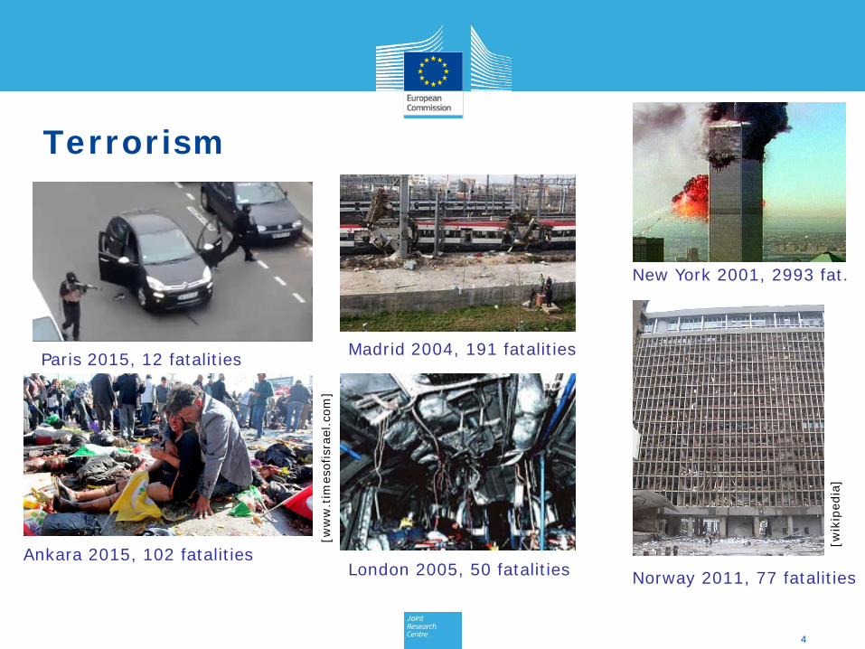
New York 2001, 2993 fat.
Madrid 2004, 191 fatalities
London 2005, 50 fatalities
Terrorism
Norway 2011, 77 fatalities
[wik
iped
ia]
4
Ankara 2015, 102 fatalities
[ww
w.t
imes
ofis
rael
.com
]
Paris 2015, 12 fatalities
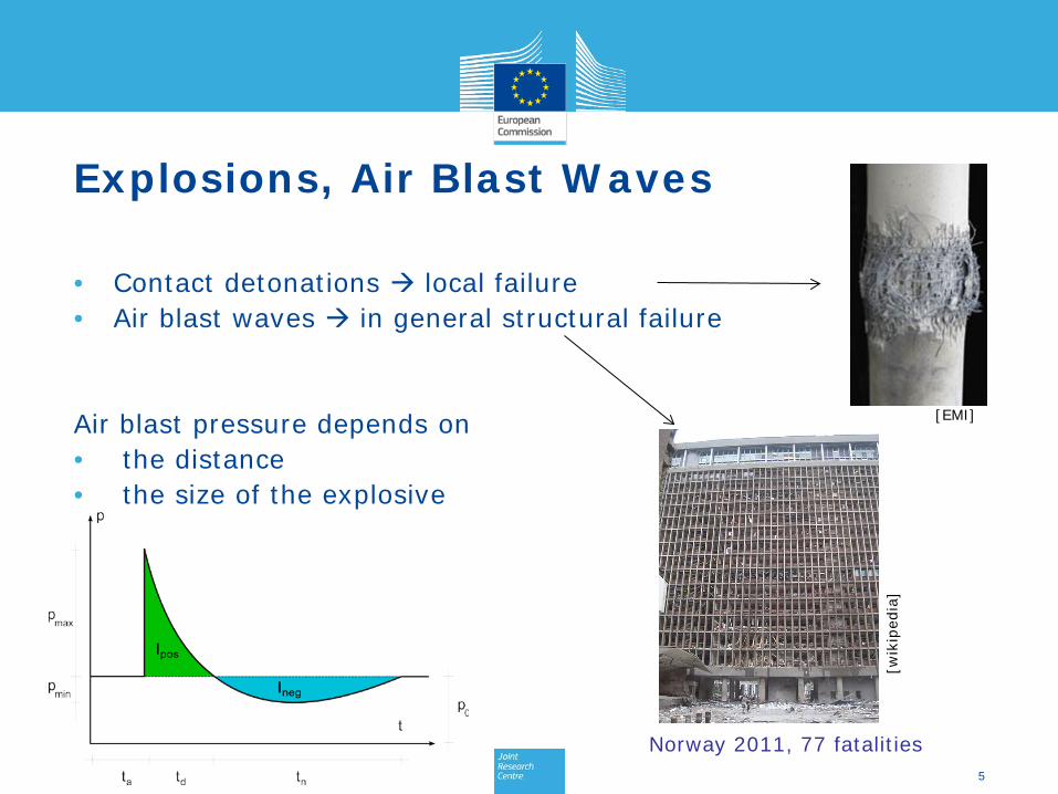
Explosions, Air Blast Waves
• Contact detonations local failure • Air blast waves in general structural failure Air blast pressure depends on • the distance • the size of the explosive
[EMI]
5
Norway 2011, 77 fatalities
[wik
iped
ia]

Experiments Model Calibration Simulations ELSA labs • Experimental setup for fast dynamic testing of materials • Experimental setup for testing small structures under blast loading
6
Simulation tool EUROPLEXUS, developed by JRC and CEA • Explicit finite element code for fast dynamic response of structures
(explosions, impacts, crashes, etc.) • Specialized in modelling of Fluid-Structure Interaction phenomena • Experience in simulation of safety problems

Blast Simulator
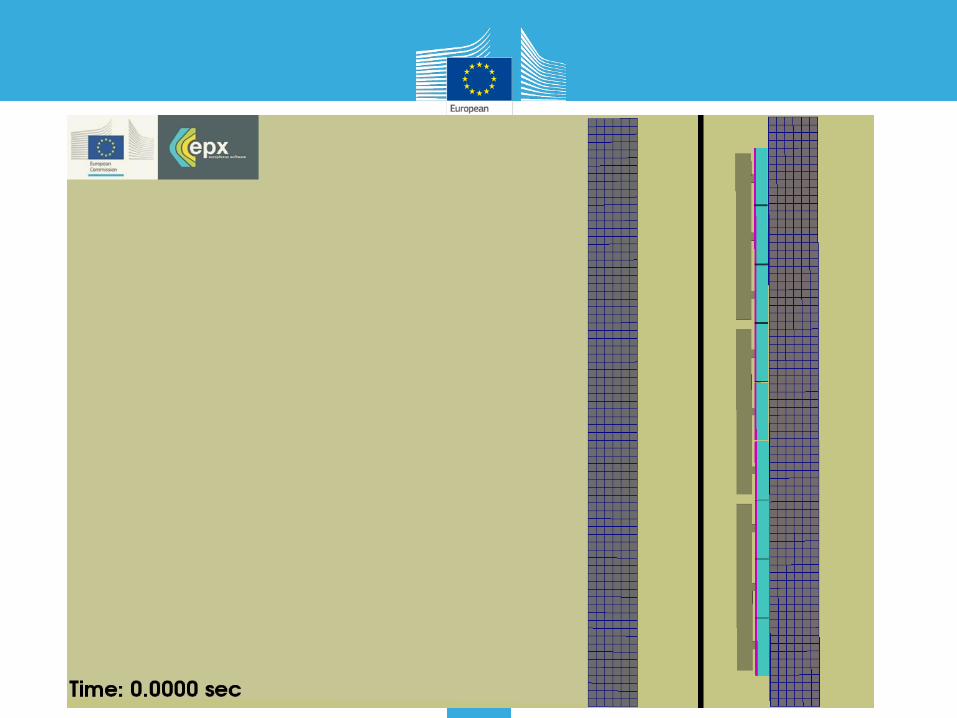

Num. Simulation /EPX
Explosion inside a station
9

Air blast loading of glass • Modern architecture uses very often big
glass surfaces • Glass most fragile part of a structure • Failure results in splinters • Air blast makes them fly into the building • Laminated glass could help to hold them
together
10
[wikipedia.org]
Railway station Liège
European Parliament, Strasbourg
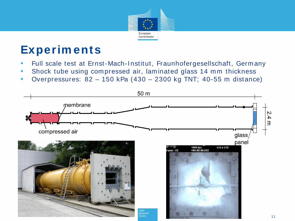
Experiments • Full scale test at Ernst-Mach-Institut, Fraunhofergesellschaft, Germany • Shock tube using compressed air, laminated glass 14 mm thickness • Overpressures: 82 – 150 kPa (430 – 2300 kg TNT; 40-55 m distance)
11
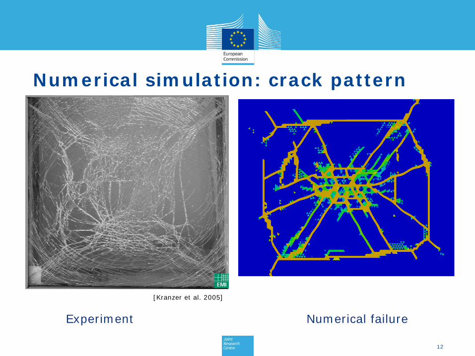
Numerical simulation: crack pattern
Experiment Numerical failure
[Kranzer et al. 2005]
12
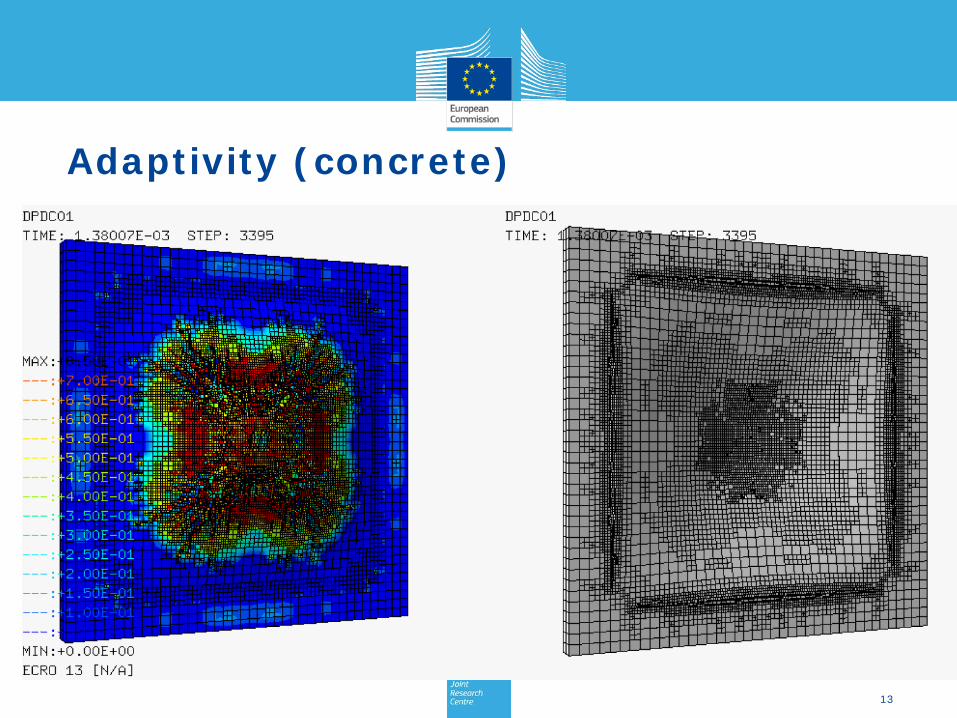
Adaptivity (concrete)
13

Aluminium foam
14

Metal tube
15

Soft targets
16
Ankara 2015, 102 fatalities
[ww
w.t
imes
ofis
rael
.com
]
• Unarmored or undefended target (wikipedia) • Explosions in urban terrain

Explicit time integration

static & quasistatic loading structural dynamics
blast & impact
nuclear & astrophysics detonations
creep & shrinkage
10-7 10-6 10-5 10-4 10-3 10-2 10-1 100 101 102 103 104 105 106 107 108 Strain rate [s-1] ε
time – strain rate – high pressures – wave propagation
Dynamic loadings - Classification

Tensile strength [Schuler 2004]
Strain rate [s-1]
Strain rate behaviour of concrete
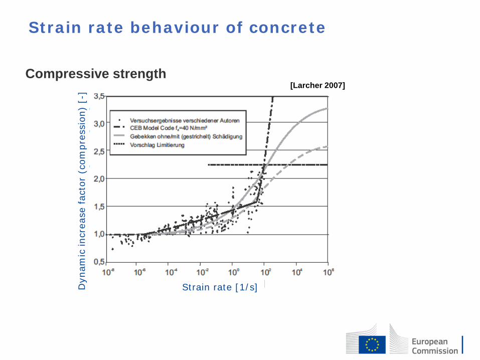
Compressive strength
Strain rate behaviour of concrete
Strain rate [1/s] Dyn
amic
incr
ease
fact
or (
com
pres
sion
) [-
] [Larcher 2007]

Strain rate effects – example: penetration of a concrete target
Experiment [Forrestal 2003]
Experiment [Forrestal 2003]
vres
60 m/s
(with DIF) (without DIF)
Material modelling
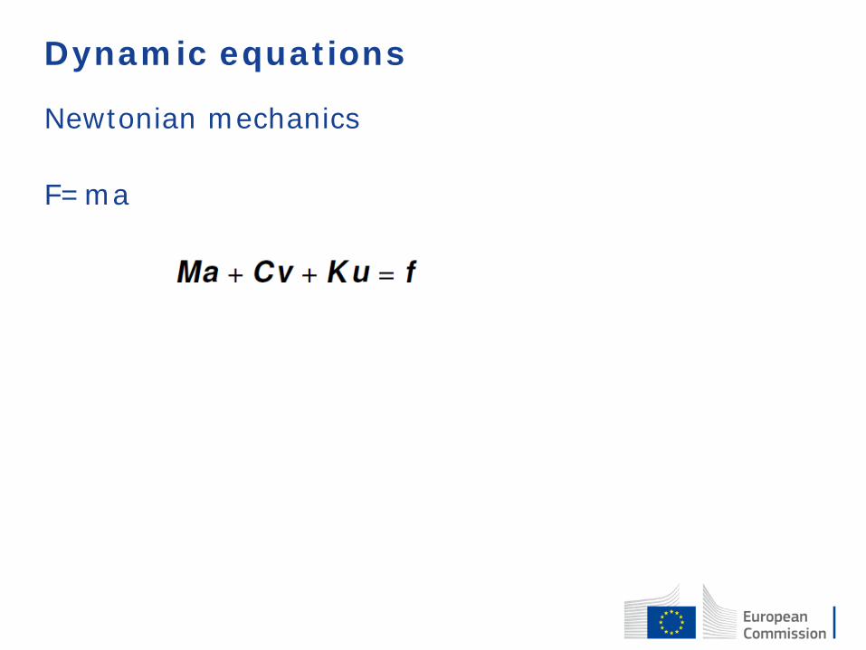
Dynamic equations
Newtonian mechanics F=ma

Newmark
Assumption for velocity and displacement:

Explicit Time Integration
Solution at t+dt is done with the values at t balance at time t No inversion of a matrix Procedure can be done on element base
Explicit Time Integration
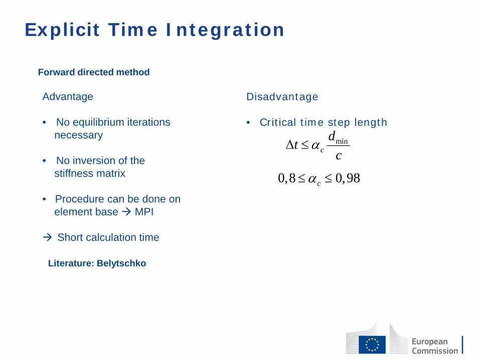
Forward directed method
Advantage • No equilibrium iterations necessary
• No inversion of the stiffness matrix
• Procedure can be done on element base MPI Short calculation time
Disadvantage • Critical time step length
0,8 0,98cα≤ ≤
minc
dtc
α∆ ≤
Literature: Belytschko
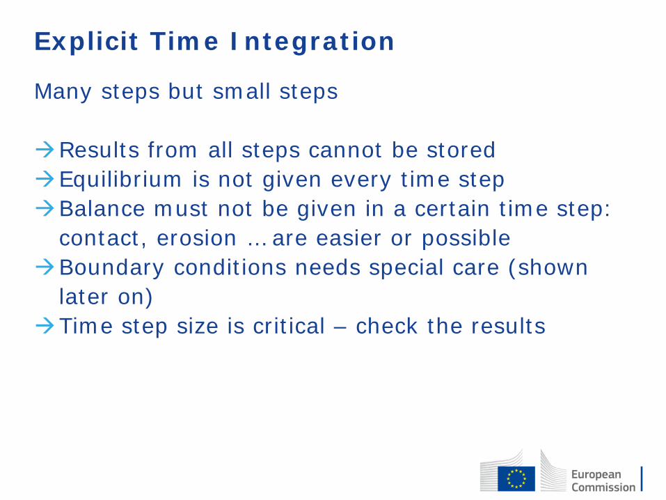
Explicit Time Integration
Many steps but small steps Results from all steps cannot be stored Equilibrium is not given every time step Balance must not be given in a certain time step:
contact, erosion … are easier or possible Boundary conditions needs special care (shown
later on) Time step size is critical – check the results
EUROPLEXUS introduction
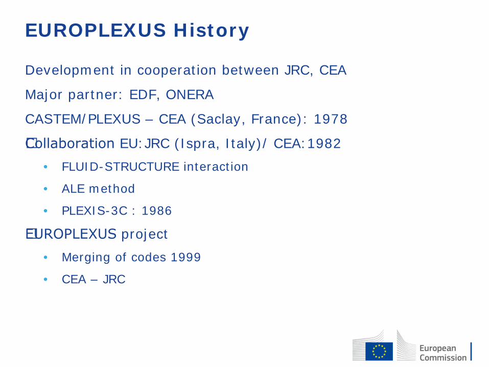
EUROPLEXUS History
Development in cooperation between JRC, CEA
Major partner: EDF, ONERA
CASTEM/PLEXUS – CEA (Saclay, France): 1978
�Collaboration EU:JRC (Ispra, Italy)/ CEA:1982 • FLUID-STRUCTURE interaction
• ALE method
• PLEXIS-3C : 1986
�EUROPLEXUS project • Merging of codes 1999
• CEA – JRC

EUROPLEXUS Licenses / principles
• Export control
• Distribution by CEA (http://www-epx.cea.fr/)
• Light version (20k stru and 200k flui), downloadable
• Education and Research: free after signing a contract, also
parts of the source for further developments
• Commercial license

General workflow
• Mesh and inputs separated • Calculation: exe
Mesh creation Calculation Post processing Input definitions
• Nodes • Elements • Groups of
nodes/elements
• Materials • Boundaries • Loading • Options
• Reading mesh and input
• Producing output
• Visualizing results

Detailed workflow
Mesh creation
Calculation
Internal Input definitions Free format
CAST3M
LS-prepost Hypermesh
Salome
ParaView
Postprocessing Geometry
Free format
CAD

Preprocessors
Objective: Create mesh (nodes, elements, groups)
CAST3M
LS-prepost Hypermesh
Salome
.msh
.k
• FE software (CEA), freely available • Mesh created by defining points, lines, surfaces etc. (script
language) • Very powerful but difficult to learn
• generic platform for Pre- and Post-Processing (open-source)
• Generic LS-DYNA k-file input
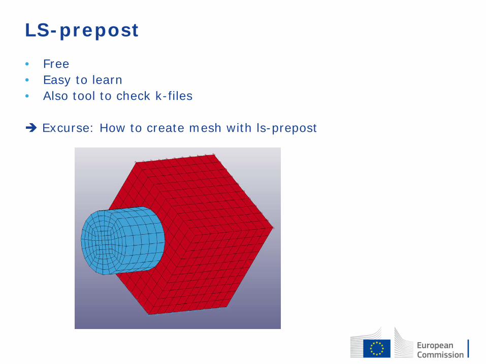
LS-prepost • Free • Easy to learn • Also tool to check k-files
Excurse: How to create mesh with ls-prepost
Organization of k-file The following keywords are supported • *NODE • *ELEMENT_SHELL • *ELEMENT_SOLID • *SET_NODE_LIST • *SET_NODE_ELEM

Postprocessors
Objective: visualize results (displacements, stress,…)
Listing
ParaView
Plots
Inte
rnal
Ex
tern
al
• Very powerful but more difficult to learn
• generic platform for Post-Processing (open-source)
Movies
Files
.epx EUROPLEXUS input file
.k LS-DYNA mesh file
.msh CASTEM mesh file
.listing General outputs
.std Error messages
.log Logging (one line per step)

EPX-Input file • *.epx file • Using groups of keywords (primary keywords) • Creating epx-file: running through the groups
A DIME PROBLEM TYPE AND DIMENSIONING
B GEOM MESH AND GRID MOTION
C COMP GEOMETRIC COMPLEMENTS
C1 MATE MATERIALS
D LINK LINKS
E INIT FUNCTIONS AND INITIAL CONDITIONS
F CHAR LOADS
G ECRI PRINTOUT AND STORAGE OF RESULTS
H OPTI OPTIONS
I CALC TRANSIENT CALCULATION DEFINITION
ED POST-TREATMENT BY EUROPLEXUS
O INTERACTIVE COMMANDS
V The built-in OpenGL Graphical Visualizer

Manual http://europlexus.jrc.ec.europa.eu/public/manual_pdf/manual.pdf (development version!) or including in the distribution Contains • Getting started • Keyword groups (A-…) • Bibliography • Index Hands on!

Units
• User defines the units in a coherent way
• Some exceptions for some materials / models
• SI units strongly recommended (m, kg, s, K)

First file!
Groups not covered here: DIME, CHAR

ParaView
• open source • multiple-platform • interactive, scientific visualization • client–server architecture • built on top of the Visualization Toolkit (VTK)
libraries • www.paraview.org
ParaView
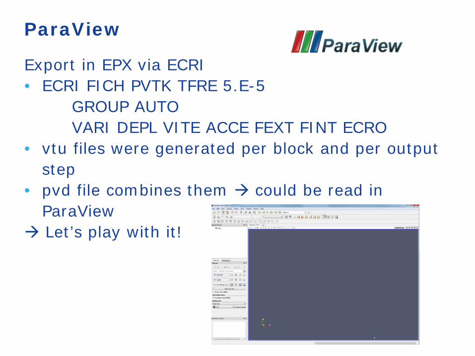
Export in EPX via ECRI • ECRI FICH PVTK TFRE 5.E-5 GROUP AUTO VARI DEPL VITE ACCE FEXT FINT ECRO • vtu files were generated per block and per output
step • pvd file combines them could be read in
ParaView Let’s play with it!
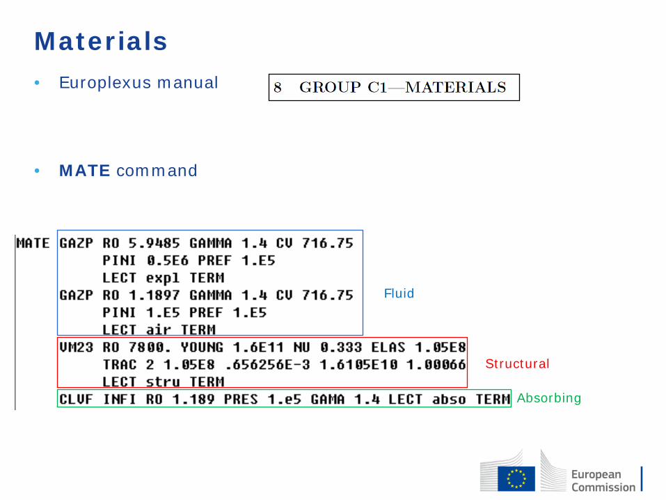
Materials • Europlexus manual
• MATE command Fluid Structural Absorbing

Materials NUMBER OF ELEMENTS TYPE 156
NUMBER OF MATERIALS TYPE 123
Material-Element combinations (from manual)

Materials NUMBER OF ELEMENTS TYPE 156
NUMBER OF MATERIALS TYPE 123

Materials (input)

Materials (types) • Structural
• Brittle (DPDC) • Ductile (VM23, VPJC,VMIS ISOT) • Hyperelastic (HYPE)
• Fluid
• Perfect gas (GAZP) • Detonation in gas mixture (GAZD, CDEM) • Water (FLUI, ADCR, SGMP) • EOS Jones-Wilkins-Lee (JWLS)
• Impedances (CLVF, IMPE) • Absorbing boundary condition for fluid mesh (ABSO, INFI) • Loading boundary conditions (AIRB, PIMP)

Materials (capabilities) • Structural
• Large displacements/strains/rotations • Plasticity • Hardening / Softening • Strain rate effect • Erosion • hyperelasticity
• Fluid
• Perfect gas • Detonation • Gas mixture • Combustion
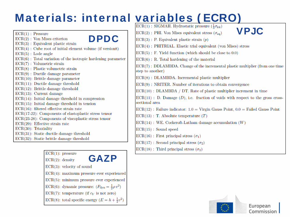
Materials: internal variables (ECRO)
DPDC
GAZP
VPJC

Elements • Europlexus manual
Type of computation
Element definition
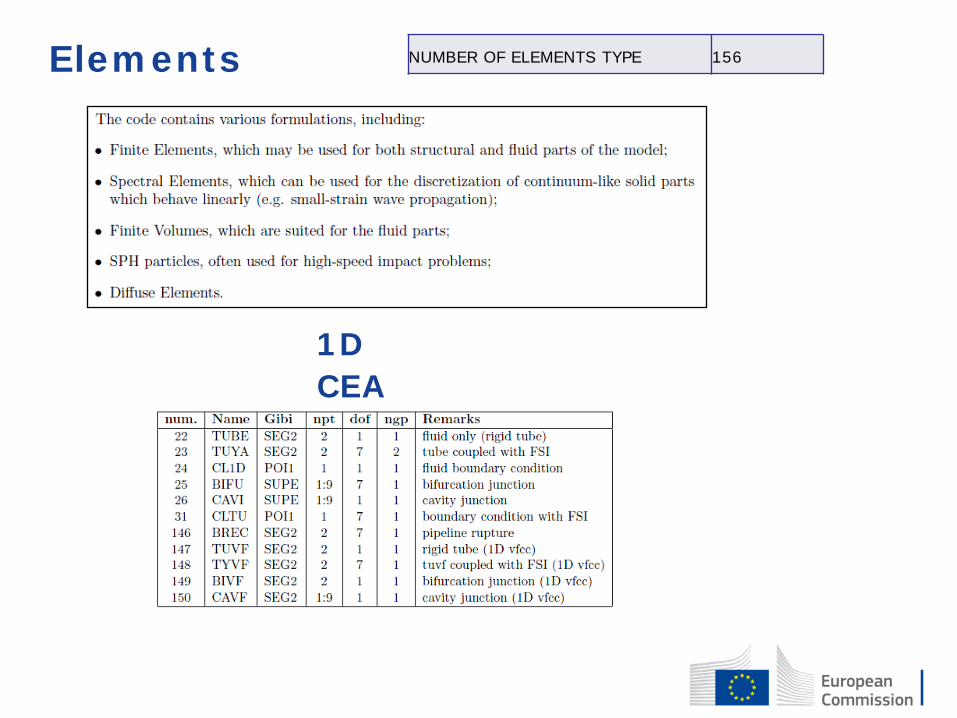
Elements
1D CEA
NUMBER OF ELEMENTS TYPE 156

Elements (2D)
CEA JRC

Elements (3D) CEA JRC

Elements (3D) • Structural
• Beam like elements (BR3D) • Shell elements (Q4GS, T3GS) • Solid elements (CUBE, CUB8, PRIS, TETR) • Material points (PMAT, DEBR)
• Fluid
• Finite volumes (CUVF, PRVF, TEVF, PYVF) • Finite elements (FL38, FL36, FL34)
• Boundary condition • Shell elements (CL3D, CL3T)
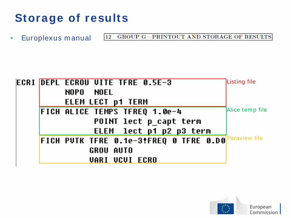
Storage of results • Europlexus manual
Listing file
Alice temp file
Paraview file
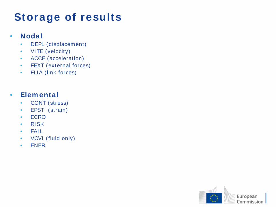
Storage of results • Nodal
• DEPL (displacement) • VITE (velocity) • ACCE (acceleration) • FEXT (external forces) • FLIA (link forces)
• Elemental • CONT (stress) • EPST (strain) • ECRO • RISK • FAIL • VCVI (fluid only) • ENER

Storage of results • Listing file (Ascii)
• Element/ node printouts with a defined output frequency • not very efficient
• Alice file (binary)
• Europlexus storage type • Can be split • Is becoming very large but contains all the desired data
• Alice temp file (binary)
• Europlexus storage type • Can be split • Very efficient but the user has to predefine the desired data
• Paraview file (binary/ascii)
• Paraview storage type (pvtk) • Very efficient for visualizing purposes

Post-processing with EPX
Create output curves
Read alice file
Print curves on a ps file
Print curves on a punch file

Post-processing with EPX - Curves • Curves • Nodal/ elemental quantities • Zone quantities • Curves as a function of space (SCOURBE) • Read a curve (RCOURBE) • Other special type of curves (PCOURBE, DCOURBE etc.) • Curves manipulation
• Integration • Summation • Max, mean, min
• Postscript file creation (TRACE) • Axis definition • Color, thickness etc. • Max, mean, min
• Punch file creation (LIST)

Post-processing with EPX
Post-script file example Punch file example

Post-processing with EPX • REGIONS (11.9)
• Group of Nodes or Elements • Monitor the quantities of a group • Energy balance or average values • Listing, punch , alice files • Be aware of the available quantities • The group has to be defined in advance • Zones solution

Interactive commands with EPX • EPX manual • CONV WIN (only for windows)
1
2
3
4
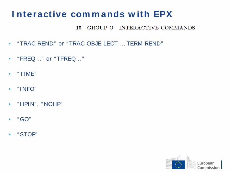
Interactive commands with EPX
• “TRAC REND” or “TRAC OBJE LECT … TERM REND”
• “FREQ ..” or “TFREQ ..”
• “TIME”
• “INFO”
• “HPIN”, “NOHP”
• “GO”
• “STOP”
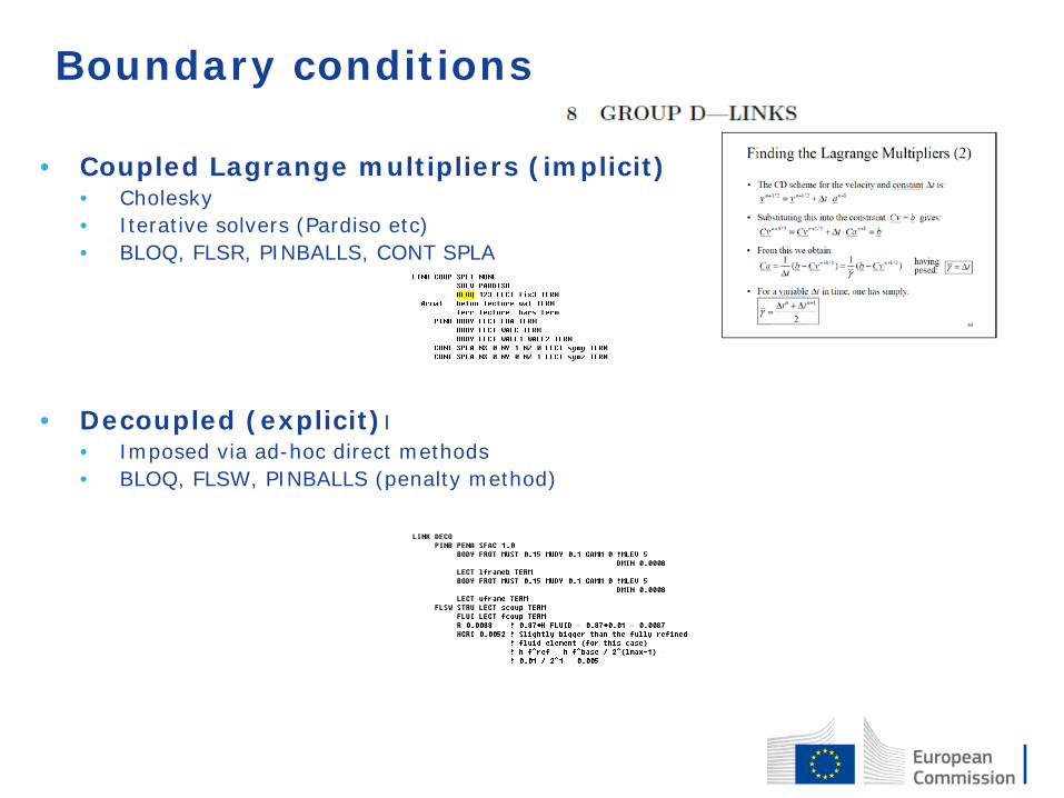
Boundary conditions
• Coupled Lagrange multipliers (implicit)
• Cholesky • Iterative solvers (Pardiso etc) • BLOQ, FLSR, PINBALLS, CONT SPLA
• Decoupled (explicit)I • Imposed via ad-hoc direct methods • BLOQ, FLSW, PINBALLS (penalty method)

Boundary conditions
• Blockages (8.5)
• Time-limited blockages (8.6)
• Symmetry conditions (8.8.6)
• Sliding (8.27, 8.48)

Fluid boundary conditions
• Absorbing boundaries
• IMPE ABSO (FE) • CLVF ABSO, INFI (VFCC) • Applied via appropriate (CL) elements
• Reflecting boundaries • Every free face in 3D or edge in 2D (for FV) • FSR for FE
Slides\videos\video2.avi Slides\videos\GFM1.avi Slides\videos\full21b2avi_01.avi
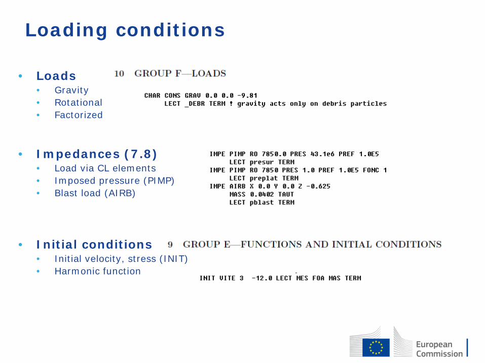
Loading conditions
• Loads
• Gravity • Rotational • Factorized
• Impedances (7.8) • Load via CL elements • Imposed pressure (PIMP) • Blast load (AIRB)
• Initial conditions • Initial velocity, stress (INIT) • Harmonic function
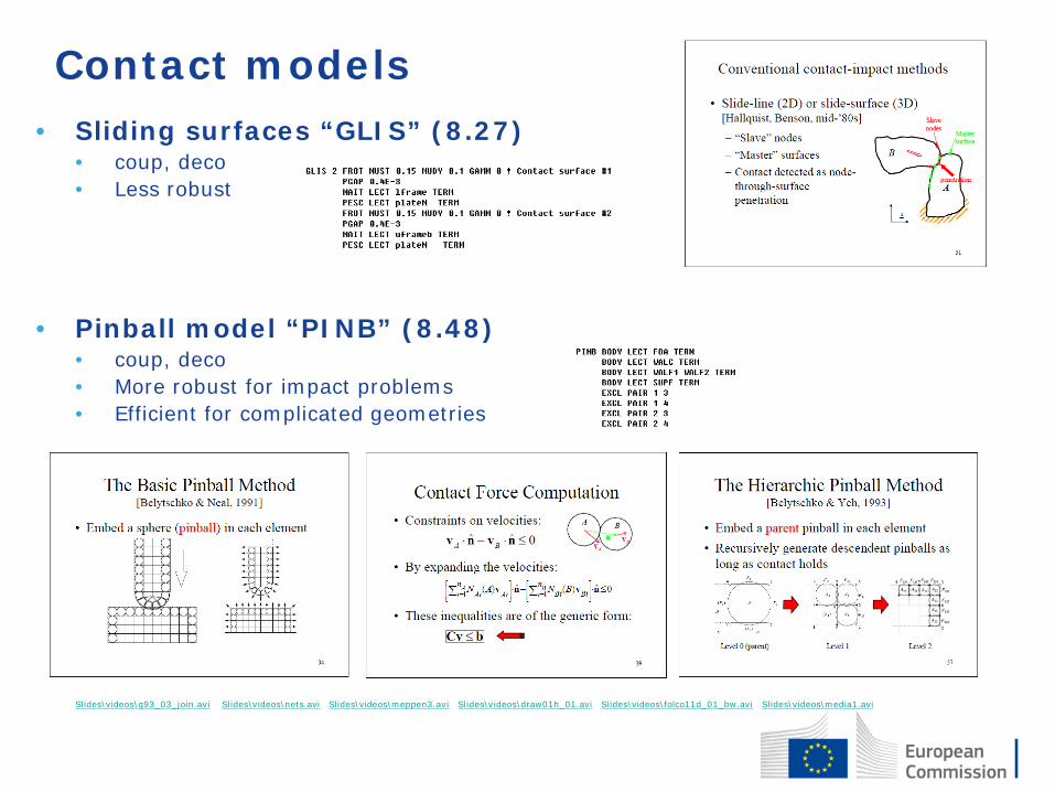
Contact models
• Sliding surfaces “GLIS” (8.27)
• coup, deco • Less robust
• Pinball model “PINB” (8.48) • coup, deco • More robust for impact problems • Efficient for complicated geometries
Slides\videos\q93_03_join.avi Slides\videos\nets.avi Slides\videos\meppen3.avi Slides\videos\draw01h_01.avi Slides\videos\folco11d_01_bw.avi Slides\videos\media1.avi

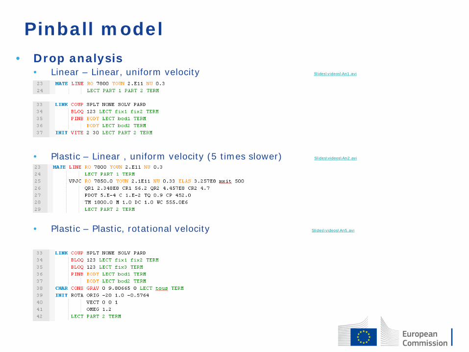
Pinball model
• Drop analysis
• 2 bodies (beams) • One fixed the other with uniform velocity • Same material different thickness
• Pinball parameters
• Hierarchy level for descendants (MLEV) • Self-contact (SELF) • Exclude pairs (EXCL)
Slides\videos\meppen3.avi Slides\videos\draw01h_01.avi Slides\videos\impex2c.avi
MLEV 0 MLEV 2
Pinball model
• Drop analysis
• Linear – Linear, uniform velocity Slides\videos\An1.avi
• Plastic – Linear , uniform velocity (5 times slower) Slides\videos\An2.avi
• Plastic – Plastic, rotational velocity Slides\videos\An5.avi

71
Impedances
Superposed elements (CL3D, CL3T) - Shell: pressure - Fluids: Absorbing boundaries Material IMPE for loading IMPE AIRB NODE LECT charge TERM MASS 1 LECT impe TERM

72
Fluid-Structure Interaction (FSI)

73
Fluid-structure interaction motivation
• Fluid behavior
• Reflections • Channeling effect • Shadowing effect
• Structural behavior
• Significant deformation • Failure and element erosion • Formation of flying debris
Slides\videos\lora15_pres.avi Slides\videos\GFM1.avi Slides\videos\gare1_comp.avi Slides\videos\BuildingBlast.avi Slides\videos\CompPreLOGOs.avi Slides\videos\train_logo.avi
74
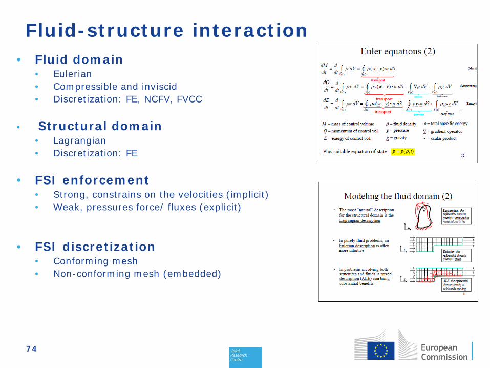
Fluid-structure interaction
• Fluid domain
• Eulerian • Compressible and inviscid • Discretization: FE, NCFV, FVCC
• Structural domain
• Lagrangian • Discretization: FE
• FSI enforcement
• Strong, constrains on the velocities (implicit) • Weak, pressures force/ fluxes (explicit)
• FSI discretization • Conforming mesh • Non-conforming mesh (embedded)

75
FSI discretization
• Conforming mesh • Medium computational cost + • Robust + • Rezoning problems – • No structural failure – • High complexity in the preparation of the mesh –
• Non-conforming mesh
• Treats cases with significant deformation (failure etc.) + • Low complexity in the preparation of the mesh + • Robust + • High computational cost – • Sensitive to the parameters of the influence domain –

76
FSI embedded model
• Automatically build up an “influence domain” around the
structure (a sphere at each S node)
• Identify (fast search) fluid nodes F currently located within the influence domain
• Impose suitable constraints on velocities : vF ∙ nS* – vS* ∙ nS* = 0 (nS* is the normal to the structure, S* is closest structural point to fluid node)
The grayed fluid nodes are coupled with the structure

77
FSI embedded model • Fluid mesh regular parallelepiped grid
• Structural mesh
• The two meshes are simply superposed
• Absorbing boundaries on the envelope of the fluid mesh

78
FSI embedded model

79
Fluid boundary conditions
• Absorbing boundaries
• IMPE ABSO (FE) • CLVF ABSO, INFI (VFCC) • Applied via appropriate (CL) elements
• Reflecting boundaries • Every free face in 3D or edge in 2D (for FV) • FSR for FE
Slides\videos\video2.avi Slides\videos\GFM1.avi Slides\videos\full21b2avi_01.avi

80
FSI Approaches (embedded)
• General
• FE for the fluid mesh – • Coupled – • Robust +
• Input • Finite El. 2D: FL24, FLUT • Finite El. 3D: FL38, FLUT • Abs. Bound. 3D: CL3Q, IMPE ABSI
81
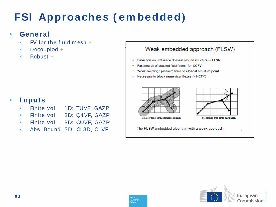
FSI Approaches (embedded)
• General
• FV for the fluid mesh + • Decoupled + • Robust +
• Inputs • Finite Vol 1D: TUVF, GAZP • Finite Vol 2D: Q4VF, GAZP • Finite Vol 3D: CUVF, GAZP • Abs. Bound. 3D: CL3D, CLVF
82
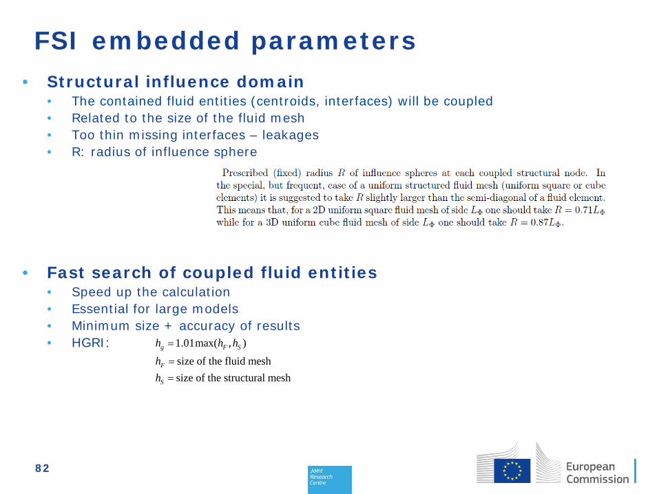
FSI embedded parameters
• Structural influence domain
• The contained fluid entities (centroids, interfaces) will be coupled • Related to the size of the fluid mesh • Too thin missing interfaces – leakages • R: radius of influence sphere
• Fast search of coupled fluid entities • Speed up the calculation • Essential for large models • Minimum size + accuracy of results • HGRI:
1.01max( , )
size of the fluid meshsize of the structural mesh
g F S
F
S
h h hhh
=
==

83
FSI Inputs
• Fluid only
- High pressure zone
- Ambient pressure zone
- Duplicated nodes (reflecting boundaries)
- Free edges (reflecting boundaries) Slides\videos\Ex2An1C.avi
84
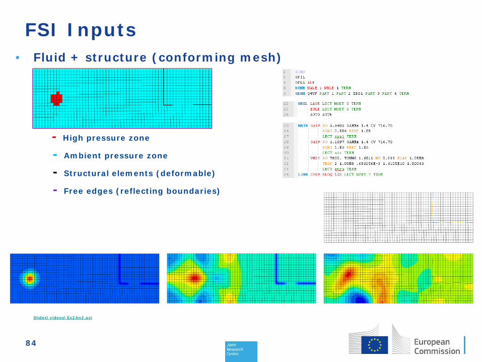
FSI Inputs
• Fluid + structure (conforming mesh)
- High pressure zone
- Ambient pressure zone
- Structural elements (deformable)
- Free edges (reflecting boundaries) Slides\videos\Ex2An2.avi
85
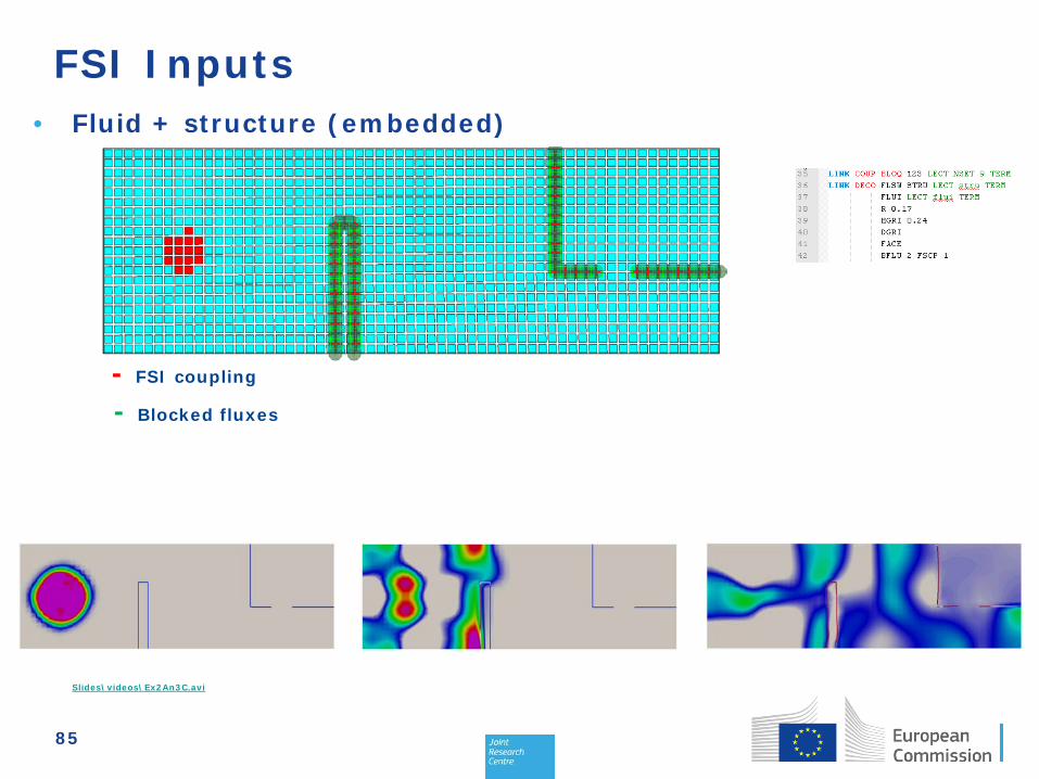
FSI Inputs
• Fluid + structure (embedded)
- FSI coupling
- Blocked fluxes Slides\videos\Ex2An3C.avi
86
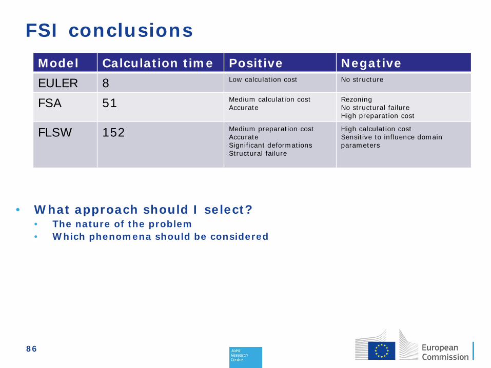
FSI conclusions
• What approach should I select?
• The nature of the problem • Which phenomena should be considered
Model Calculation time Positive Negative EULER 8 Low calculation cost No structure
FSA 51 Medium calculation cost Accurate
Rezoning No structural failure High preparation cost
FLSW 152 Medium preparation cost Accurate Significant deformations Structural failure
High calculation cost Sensitive to influence domain parameters
87
Failure / Erosion / Debris

88
Failure / erosion
• Failure: reaching a certain criteria in an IP • Erosion: removing an element from the
calculation
Failure: material behaviour: • Damage • Plastic strain • Pressure • …

89
Failure (VM23)
VMIS Von Mises stress (isotropic criterion) PEPS for a criterion based upon the principal strain PRES for a criterion based upon the hydrostatic stress PEPR for a criterion based upon the principal strain if the hydrostatic stress is positive (traction): if the hydrostatic stress is negative (compression) there is no failure.

90
Erosion • Material has reached a failure mode (damage or other criteria) • element distorted (cannot be treated any more) (CROI) • time step size is too small (CALC TFAI) • Parts of the model should be removed at a certain time step or due
to further criteria (displacement erosion, fantome elements) • Erosion of attached element (CLxx)
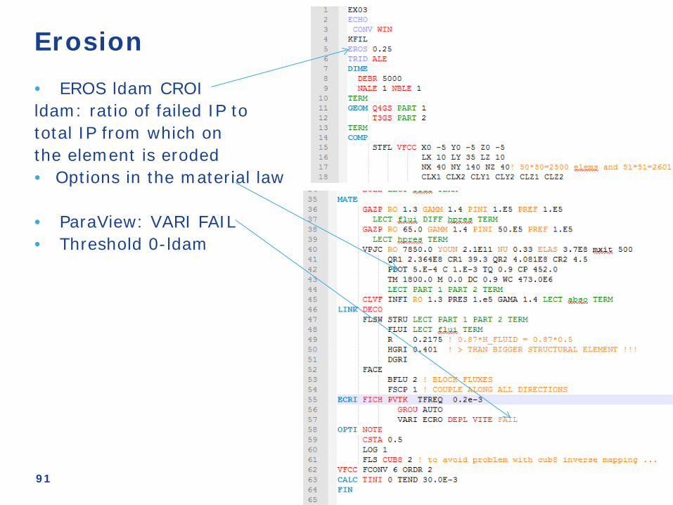
91
Erosion • EROS ldam CROI ldam: ratio of failed IP to total IP from which on the element is eroded • Options in the material law
• ParaView: VARI FAIL • Threshold 0-ldam
92
Flying debris • Idea: material is in reality not eroded but mainly resulted in
fragments • Transferring the eroded elements in fragments • Fragments were simple material points but could also be embedded
in a fluid • Drag forces and gravity could be added • DEBR must be dimensioned at the beginning • General debris parameters • Creation of the debris

93
Example

94
FSI Inputs 3D explosion
• Explosion of tank in open field
• Embedded FLSW • Flaw inserted via a thicker element • STFL fluid mesh construction
flaw
origin LY
LX
LZ
CLZ2
CLX1
CLY2

95
FSI Inputs 3D explosion
• Explosion of tank in open field
Debris definition
Flaw definition
FSI parameters definition

96
FSI Inputs 3D explosion
• Explosion of tank in open field
• Results
• Slides\videos\Ex3An1C.avi
97
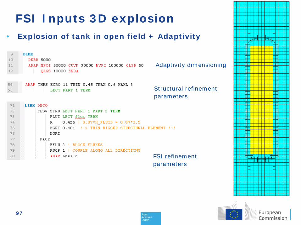
FSI Inputs 3D explosion
• Explosion of tank in open field + Adaptivity
Structural refinement parameters
Adaptivity dimensioning
FSI refinement parameters

98
FSI Inputs 3D explosion
• Explosion of tank in open field + Adaptivity
• Results
Slides\videos\Ex3An2.avi

99
Mesh Adaptivity

100
Mesh adaptivity
• Local refinement of the mesh
• On some zones that considered as critical • Reduce the size of the model • High level of accuracy
101
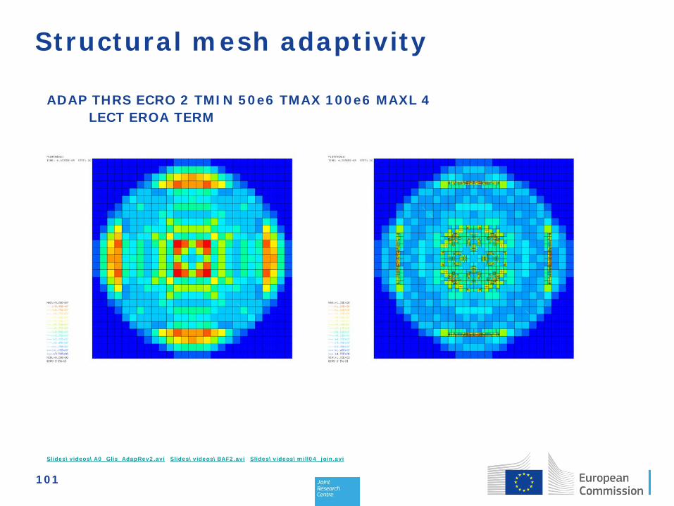
Structural mesh adaptivity
ADAP THRS ECRO 2 TMIN 50e6 TMAX 100e6 MAXL 4 LECT EROA TERM
Slides\videos\A0_Glis_AdapRev2.avi Slides\videos\BAF2.avi Slides\videos\mill04_join.avi

102
Structural mesh adaptivity
• Crack formation with damage driven adaptivity
• Indicator should be a damage parameter • No unsplit since the damage parameter is a cumulative quantity
• Slides\videos\A0_Glis_AdapRev2.avi Slides\videos\BAF2.avi
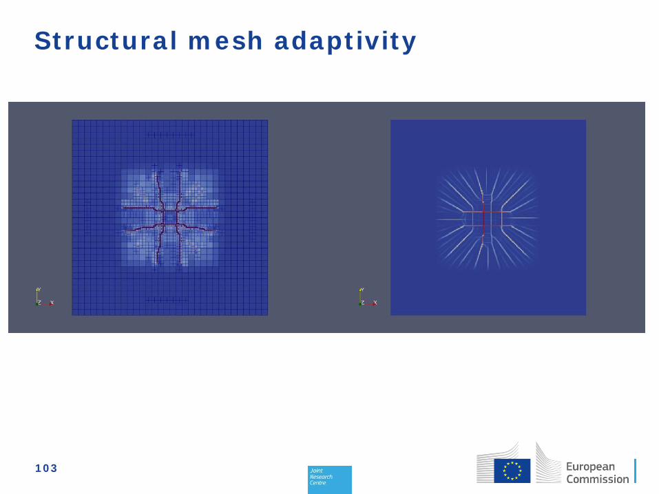
103
Structural mesh adaptivity
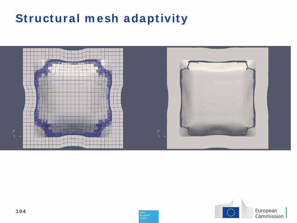
104
Structural mesh adaptivity

105
Structural mesh adaptivity

106
Structural mesh adaptivity
107
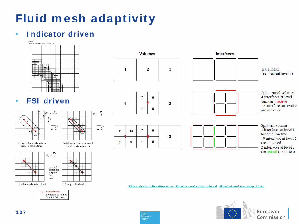
Fluid mesh adaptivity
• Indicator driven
• FSI driven
Slides\videos\fullAdaPresavi.avi Slides\videos\mill04_join.avi Slides\videos\test_adap_3d.avi

108
Mesh adaptivity
• Advantages
• Less elements less the calculation cost
• Decrease the memory requirements for the calculation
• The size of the output files can decrease significantly
• We can have a period with higher time step

109
FSI Inputs 3D explosion
• Explosion of tank in open field
• Results
• Slides\videos\Ex3An1C.avi

110
FSI Inputs 3D explosion
• Explosion of tank in open field + Adaptivity
Structural refinement parameters
Adaptivity dimensioning
FSI refinement parameters
111
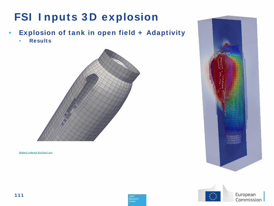
FSI Inputs 3D explosion
• Explosion of tank in open field + Adaptivity
• Results
Slides\videos\Ex3An2.avi

112
Combustion

Combustion (burning)
• Chemical reaction between a fuel and oxidant • Producing oxidized, often gaseous products
Explosions: Detonation – deflagration • Reaction speed – speed of sound Hydrogen explosions EUROPLEXUS: 2 material models GAZD and CDEM

Material models
• Euler equations (compressible, inviscid flow) for a mixture of perfect gases in detonation regime
• Chemical reaction represented by combustion of the hydrogen
• Associated kinetics taken into account • Underlying equations: conservation of mass,
momentum and energy, plus the equations of state of the materials and the relations describing the chemical reaction

Material models
After a certain delay interval dT (measured from the instant at which a certain critical temperature T is reached) combustion starts releasing a certain amount of energy q into the system
Material models – GAZD CDEM
• GAZD specific for detonation • CDEM can be used for a wider range (strong
detonation to weak deflagration) • CDEM More general • CDEM More expensive • Course concentrates on CDEM

Material models CDEM
• At least two zones are needed: burnt and unburnt • Each definition has two parts: general and
components
General
Components

Material models CDEM • PINI: pressure • PREF: reference pressure (1 bar) • TINI: initial temperature • KSIO: Initial volume fraction, number close to 1 but not 1.0 • K0: flame speed, chosen high, theoretical value is used • TMAX: max temperature at which the polynomial expression giving the heat
capacity at constant volume • R: gas constant (8.314 J/(mol K)) • NESP: number of components • ORDP: order of the polynomial equation • NLHS: number of reactants (H2 and O2)
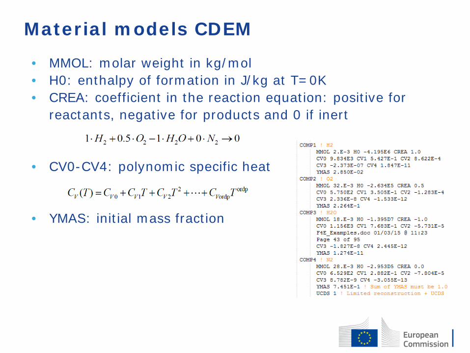
Material models CDEM
• MMOL: molar weight in kg/mol • H0: enthalpy of formation in J/kg at T=0K • CREA: coefficient in the reaction equation: positive for
reactants, negative for products and 0 if inert
• CV0-CV4: polynomic specific heat
• YMAS: initial mass fraction

Material models CDEM: output (ECRO)
Numbering very difficult – numbering written in the listing, for 3D: • 1: pressure of the mixture • 2: density of the mixture • 3: maximum sound speed • 4: Volume fraction of unburnt • 5: density of unburnt • 6: x-velocity of unburnt • 7: y-velocity of unburnt • 8: z-velocity of unburnt • 9: pressure of unburnt • 10: Volume fraction of burnt • 11: density of burnt • 12: x-velocity of burnt • 13: y-velocity of burnt • 14: z-velocity of burnt • 15: pressure of burnt • 22: FUNDAMENTAL FLAME SPEED • 23: ABSOLUTE TEMPERATURE OF THE MIXTURE …

Options
Several options
• In particular for finite volume solution

Easy input (!)
Definition of CDEM material only once for all parts Some values were overwritten later on The different parts are defined with the INIT
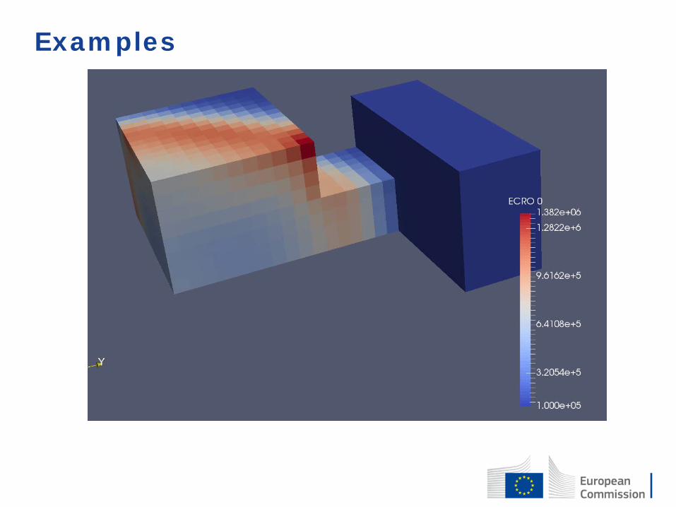
Examples


