Is Mandatory Voting Better than Voluntary Voting?
Stefan Krasa Mattias Polborn∗
May 22, 2008
Abstract
We investigate the welfare effects of policies that increase voter turnout in costly
voting models. In a generalized costly voting model, we show that if the electorate
is sufficiently large, then increasing voter turnout is generically efficient. Increasing
turnout in small elections is only inefficient if the electorate is evenly divided or if
there is already almost complete voter participation. Finally, we argue that the effects
underlying our results are robust in a large class of endogenous participation models.
JEL Classification Numbers: C70, D72.
Keywords: Costly voting, mandatory voting, compulsory voting, externalities
∗Address of the authors: Department of Economics, University of Illinois, 1206 South 6th Street, Cham-
paign, IL 61820 USA,
E-mails: [email protected], [email protected].
We thank seminar audiences at Northwestern, Maastricht, the 2005 Canadian Economic Theory Confer-
ence, the 12th Wallis conference at the University of Rochester and Dan Bernhardt, Rob Clark and Matthias
Messner for valuable suggestions and comments. Stefan Krasa gratefully acknowledges financial support
from National Science Foundation grant SES-031839. Any opinions, findings, and conclusions or recom-
mendations expressed in this paper are those of the authors and do not necessarily reflect the views of the
National Science Foundation or any other organization.
1 Introduction
Many societies encourage voter participation in elections and meetings. In the recent 2004
U.S. elections, many states expanded the opportunities for early and absentee voting. Several
other countries have tried to increase turnout by making participation in elections “manda-
tory”.1 For example, the Australian parliament enacted mandatory voting in 1924, because
voter turnout had dropped below 60 percent. By law, all Australian citizens over the age
of 18 must register to vote and show up at a polling place on election day. A citizen who
misses the election is subject to a $15 fine.2 The Australian mandatory voting law is suc-
cessful in increasing voter turnout above 90%.3 Supporters of mandatory voting see voting
as a civic duty similar to paying taxes, and argue that a higher level of participation in-
creases the legitimacy of government. “The most important [argument] is that compulsory
voting ensures that government does indeed represent the will of the whole population, not
merely the section of the population that decides to express their opinions” (Wikipedia,
http://en.wikipedia.org/).
Relatedly, political scientists and political commentators often deplore participation rates
in US elections as “too low” and advocate steps to increase turnout (e.g. Olbermann (2002),
Dean (2003) and Weiner (2004)). A more unusual proposal was the Arizona Voter Reward
Act, proposing to award 1 million dollars to a randomly selected citizen who voted, with the
objective to increase the participation rate.4 Yet, beyond the claim that higher participation
would confer a greater legitimacy on the elected government, there are no solid economic
arguments why increased turnout should be desirable. Providing such an argument is the
main contributions of this paper.
We use a costly voting model to investigate whether policies that increase voter turnout
are socially beneficial. Specifically, we address the following questions: Does fining non-
voters (or, equivalently, subsidizing voters) alter election outcomes, relative to voluntary
voting? If election outcomes are affected, and if subsidized voting improves social decisions,
do these benefits outweigh the increased voting costs that are a consequence of higher voter
turnout?
1These include most South American countries, as well as Australia and several European and Asian
countries. See, for example, Wikipedia http://en.wikipedia.org/wiki/Compulsory voting for a list.2All non-voters receive a letter asking them to pay the fine. Instead of paying the fine, non-voters can
also provide a written excuse. Thus, the actual cost of non-voting is the minimum over the disutility of
paying $15 or writing the letter (see Weiner (2004) for details).3There were a few experiments with mandatory voting laws before 1900 in the US. In 1896, the Supreme
Court of Missouri struck down a Kansas City charter provision as unconstitutional that assessed a $2.50 poll
tax on every man twenty-one years of age or older who failed to vote in the general city election. See Dean
(2003).4This proposal was voted on in a November 2006 referendum and failed to get a majority.
1
Our model builds on the costly voting literature (Ledyard (1984), Palfrey and Rosenthal
(1983), Palfrey and Rosenthal (1985), Borgers (2004), Goeree and Grosser (2007)). N citizens
must decide between two candidates A and B. Each citizen’s preference is private information
and independently drawn from a common distribution that assigns probability α to being
an A-supporter (and 1−α to being a B-supporter). In addition, each individual has private
information about his voting cost c. The parameter α is drawn at an interim stage, so
that individuals know α when they decide whether or not to vote. For example, potential
voters can learn α from pre-election opinion polls. However, institutional choices (e.g.,
whether voting should be mandatory) cannot be conditioned on the realization of α, because
institutional choices apply for a longer time period than just a single issue election, and a
rule that explicitly conditions on α (say, “choose A without an election if α > 12”) would
likely lead to large controversies among A and B-supporters as to what α is.
We characterize conditions when voting should be encouraged and when voting should
be discouraged, and show that the former is much more likely to occur in practice. We
show that voting should be encouraged, if the expected absolute size of the two candidates’
supporter groups are sufficiently different, which occurs generically if the number of citizens
is large. We also show that the optimal policy is to pay a subsidy equal to the minimal voting
cost as the size of the electorate goes to infinity. While we derive our main results in a simple
costly voting model, we argue in Section 4 that our findings that voting should be encouraged
applies more generally to endogenous participation models in which cost considerations are
important at least for the marginal voters, or for leaders who can induce some followers to
vote.
To understand the intuition for our results, suppose that α > 0.5, i.e., it is more likely that
A-supporters are in the majority. However, in equilibrium, the probability that candidate
B wins must be sufficiently large, otherwise voters would have no incentive to participate.
For this to occur, the participation rate by B supporters must exceed that of A-supporters,
which, in turn, implies that the (expected) proportion of A-supporters among non-voters
is even higher than α. If a particular A-supporter votes and is pivotal, then he imposes
a positive externality on non-voters who support A, and a negative externality on non-
voters who support B. The net change in surplus for non-voters is approximately 0.5 (the
utility change for an individual citizen) times the difference between the number of A and
B supporters among non-voters. This change in surplus is positive, because in expectation
there are more A than B-supporters among non-voters. In contrast, the externality on voters
is negative: There are two configurations in which our A supporter is pivotal. First, if the
number of other A-voters equals the number of other B-voters, and second, if the number of
other A-voters is one smaller than the number of other B-voters. In the first case there is no
externality, while in the second case the net change in surplus is -0.5. Thus, our A supporter
2
increases surplus by voting, unless there are either almost no non-voters or the electorate is
fairly evenly split (α close to 0.5). Subsidies encourage more A than B supporters to vote,
because there are more A-supporters than B-supporters among the whole population, and
in particular, among non-voters), and are therefore welfare improving.
In an important paper, Borgers (2004) has analyzed optimal voter participation policies.
In his model, the expected number of A and B supporters are equal, which corresponds to
the special case α = 0.5 (with certainty) in our model. As a consequence, only the negative
externality occurs in Borgers’ model, implying that voluntary voting dominates mandatory
voting.
The costly voting literature dates back to Ledyard (1984) and Palfrey and Rosenthal
(1983), Palfrey and Rosenthal (1985). Empirical evidence confirms many comparative static
predictions of the costly voting model (see Blais (2000), Shachar and Nalebuff (1999), Levine
and Palfrey (2007)): In particular, minority supporters are more active in equilibrium, and
the overall participation rate is higher the closer α is to 0.5. A problem with the simple
costly voting model, however, is the unrealistic prediction of a zero participation rate in very
large elections. More sophisticated endogenous participation models combine cost consider-
ations with “ethical” voters (Feddersen and Sandroni (2006)) or introduce leaders, who can
influence the participation decision of a large number of citizens (e.g., Shachar and Nale-
buff (1999), Herrera and Martinelli (2006)). These models succeed in generating positive
participation in large electorates, while preserving the nice comparative static results of the
costly voting model. While we derive our results in a simple costly voting model, we argue
in Section 4 that they are robust in a considerably larger class of endogenous participation
models, including the ones just mentioned.
Our model is closest to Goeree and Grosser (2007), who generalize Boergers’ model to
allow for the ex-ante expected support of candidates to differ. In contrast to our paper, they
assume that the voting cost is deterministic and equal for all voters. In this framework,
they consider the effect of opinion polls that provide the electorate with better information
about the expected support of candidates. They show that an opinion poll is undesirable,
because it decreases expected turnout and this, as in our model, leads to a higher probability
of electoral mistakes. In contrast to our paper, voting subsidies in order to increase turnout
directly would be either ineffective or lead to full participation in their setup.5 In summary,
our model can be understood as a convex combination of the costly voting models of Borgers
(2004), with whom we share the assumption of stochastic voting costs, as well as the focus
of the analysis on optimal participation, and Goeree and Grosser (2007), who also analyze
the effects of asymmetry in the candidates’ support (but focus on the informational role of
polls).
5Goeree and Grosser (2007) do not analyze the effect of voting subsidies.
3
Some other recent papers study costly voting environments related to our model. Camp-
bell (1999) shows that, if voting costs of A and B supporters are drawn from different
distributions, then the candidate with the more favorable cost distribution wins almost cer-
tainly in large elections, rather than the candidate preferred by the majority. We assume
that A and B supporters’ cost of voting are drawn from the same distribution and therefore
Campbell’s effect is absent in our model.
Ghosal and Lockwood (2004) analyze a model in which voluntary participation can be
inefficiently low, but the cause of this inefficiency differs from ours. In their model, each
individual has both a “private value” preference for one of the politicians, and a “common
value” preference to select the politician who matches the unknown state of the world. When
the common value component is sufficiently important, participation by more people leads
to better information aggregation, which creates a positive externality that citizens do not
internalize.
In subsequent work, Taylor and Yildirim (2006) further analyze the costly voting model
used in this paper and derive conditions under which the symmetric equilibrium is unique.
They also derive the speed of convergence to the winning probabilities of 1/2 as the voting
population converges to infinity.
2 Model
There are N citizens who have the right to vote for one of two candidates, A or B. The
probability α that a citizen prefers candidate A to candidate B is chosen by nature according
to a probability density function g(α), and becomes public information before the election.
For example, the public information about α could be the result of pre-election opinion
polls. Preferences for candidates A and B, respectively, are then drawn independently across
individuals according to probability α.
Participating in the election is costly. The cost c a citizen pays if and only if he votes is
drawn independently according to probability density function f(c). We assume that f(c) is
strictly positive on its support [c, c], where 0 < c < 0.5. (If c > 0.5, then it is easy to show
that no citizen would ever vote). We write F (c) for the corresponding cumulative distribution
function. The outcome of the election is determined by majority rule. In case of a tie, each
candidate wins with probability 12. Citizen i receives a benefit normalized to 1 if his preferred
candidate is elected, and 0 if the other candidate wins. We allow the government to encourage
voting via a subsidy s that is paid to all voters. The subsidy s can be interpreted either as
actions by government that reduce citizens’ costs of electoral participation, or equivalently,
as a fine that non-voters must pay. Because mandatory voting laws cannot force individuals
to vote, but rather encourage participation through fines imposed on abstainers, our notion
4
of subsidized voting corresponds to how mandatory voting laws work in practice. Formally,
if Pi ∈ {A, B} is i’s preferred candidate, if E is the candidate who is elected, and if vi = 1
and vi = 0 is i’s decision whether or not to vote, then i’s utility is given by
u(E, vi; Pi, ci) =
1 − vi(ci − s) if E = Pi;
−vi(ci − s) if E 6= Pi.
There are two interesting special cases encompassed in this framework of subsidized
voting. First, if s = 0, we have a standard costly voting model; we call this case voluntary
voting. Second, if s ≥ c, then all citizens vote, and we talk of compulsory voting.
3 Results
First note that if an individual votes, his weakly dominant strategy is to vote for his preferred
candidate, and it is therefore sufficient to focus solely on an agent’s participation decision. In
Proposition 1, we show that there exists a symmetric equilibrium in pure strategies, which is
characterized by a simple cutoff value rule for the voting costs: A-supporters choose to vote
if and only if their voting costs are no higher than cA, and B-supporters have an analogous
cost threshold cB. The proofs of all propositions are in the Appendix.
Proposition 1 There exists a symmetric equilibrium in pure strategies that is characterized
by cutoff values cA and cB such that individual i votes for his preferred candidate Pi if
ci ≤ cPi, and abstains otherwise.
While the equilibrium is the unique symmetric equilibrium in all of our numeric examples,
this is very hard to prove for a general distribution of voting costs. However, in Proposition 3,
we provide conditions under which symmetric equilibria are unique, and the welfare effects
of subsidies analyzed in Propositions 4 and 5 hold for all symmetric equilibria.
We now analyze the welfare impact of voting subsidies. Welfare is the sum of citizens’
payoffs from the elected candidate minus the voting costs of those citizens who vote. For-
mally, let S(a, N, kA, kB) be the social surplus in a population with N citizens, a of whom
prefer candidate A, and let kA and kB be the number of A and B voters.
S(a, N, kA, kB) =
a − kAE(c|c ≤ cA) − kBE(c|c ≤ cB) if kA > kB
12a + 1
2(N − a) − kAE(c|c ≤ cA) − kBE(c|c ≤ cB) if kA = kB
N − a − kAE(c|c ≤ cA) − kBE(c|c ≤ cB) if kA < kB
5
Ex-ante expected welfare is then given by
W =N
∑
a=0
a∑
kA=0
N−a∑
kB=0
(
N
a
)
αa(1 − α)N−aS(a, N, kA, kB)× (1)
(
a
kA
)
F (cA)kA[1 − F (cA)]a−kA
(
N − a
kB
)
F (cB)kB [1 − F (cA)]N−a−kB ,
which is the probability that there are a A-supporters, kA A-voters and kB B-voters, multi-
plied with the conditional expected social surplus, and summed over all possible realizations.
Subsidy payments do not enter the definition of welfare directly, because they are trans-
fers between citizens and therefore drop out. Instead, subsidies affect welfare indirectly by
changing the participation choices, which may affect both the total voting costs incurred
and the electoral outcome. Note that, if subsidies had to be raised through distortionary
taxation, then the excess burden of taxation would need to be taken into account when
calculating the optimal subsidy. In this case, it also matters whether voting is encouraged
(through the payment of a subsidy to voters), or whether non-voting is discouraged (through
a penalty that non-voters have to pay). Clearly, since penalty payments can be used to re-
place some distortionary taxes, they are preferable to the payment of a subsidy, which would
create the need for additional distortionary taxation.
Proposition 2 considers small electorates in which all citizens vote as long as the numbers
of A and B supporters are sufficiently close.
Proposition 2 Suppose that c <(
N−1⌊(N−1)/2⌋
)
2−N . Then there exist δ > 0 such that
1. For all α ∈ [0.5−δ, 0.5+δ] there exists an equilibrium with full participation. Subsidies
have no effect on this equilibrium.
2. For α /∈ [0.5 − δ, 0.5 + δ] but close to 0.5 − δ and 0.5 + δ, there exists a symmetric
equilibrium with close to full participation, for which subsidies strictly lower welfare.
That is, let W (c1, c2) denote the welfare of equilibrium (c1, c2) as defined in (1). Then
there exists ε > δ and a continuous equilibrium selection e : [0.5 − ε, 0.5 + ε] × R+ →[c, c]2, such that welfare W (e(α, s)) is strictly decreasing in s for all α ∈ [0.5− ε, 0.5 +
ε] \ [0.5 − δ, 0.5 + δ].
If all agents participate, then subsidies have no effect, because cA and cB do not change.
However, once α becomes sufficiently large (or sufficiently small), some citizens no longer
vote. In this case, voters impose a negative externality on other voters, which is essentially
Borgers’ effect. In addition, because the expected number of non-voters is small, this is the
only effect that matters.
While Proposition 2 characterizes conditions under which voting subsidies may be detri-
mental for intermediate values of α, Proposition 3 shows that subsidies are beneficial for
sufficiently high values of α.
6
Proposition 3 There exists α2 < 1 such that there is a unique symmetric equilibrium for
all α ∈ (α2, 1]. Further, ∂W∂s
|s=0 > 0 for all α ∈ (α2, 1], where W is welfare defined by (1).
Thus, a voting subsidy, starting at s = 0, is welfare improving. The marginal per-capita
benefit ∂(W/N)∂s
|s=0,α=1 goes to 1 as N → ∞.
The intuition for the positive effect of subsidies is as follows: For α close to 1, (almost) all
individuals agree which candidate they prefer. However, every citizen would like other citizen
to incurs the voting cost, so that issue of participation is essentially equal to the problem
of private provision of a public good, with the associated free-riding problem among the
majority.6 To provide any incentive to participate, there must be a positive probability that
nobody votes. A voting subsidy increases expected participation and therefore reduces the
risk of a wrong decision.
We also show, in the proof of the proposition, that the per-capita welfare effect of the
subsidy converges to 1 as N → ∞ (when α is close to 1). This means that subsidies are
very effective, i.e., a unit of subsidy provided to voters raises each citizen’s welfare by one
unit. When N is sufficiently large, then there is a severe free-rider problem and only very
few agents vote. To provide an incentive for the lowest cost agent to vote, the equilibrium
probability of a mistake must be (c − s), because avoiding such a mistake is the benefit
of voting. Expected average welfare in equilibrium is given by 1 minus the probability of
mistake. An increase in s one-to-one reduces the probability of a mistake, without leading
to a significantly higher per capita participation cost.
0.5 0.6 0.7 0.8 0.9 1-0.2
0
0.2
0.4
0.6
0.8
1
1.2
aa
N=20 N=80 and N=320
0.5 0.6 0.7 0.8 0.9 1-0.5
0
0.5
1
1.5
2
2.5
n=80
n=320
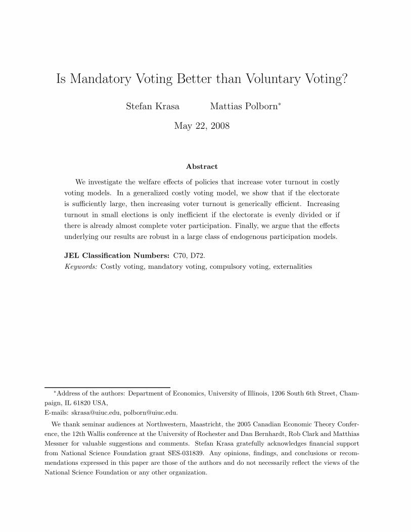
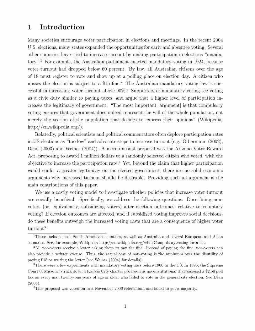
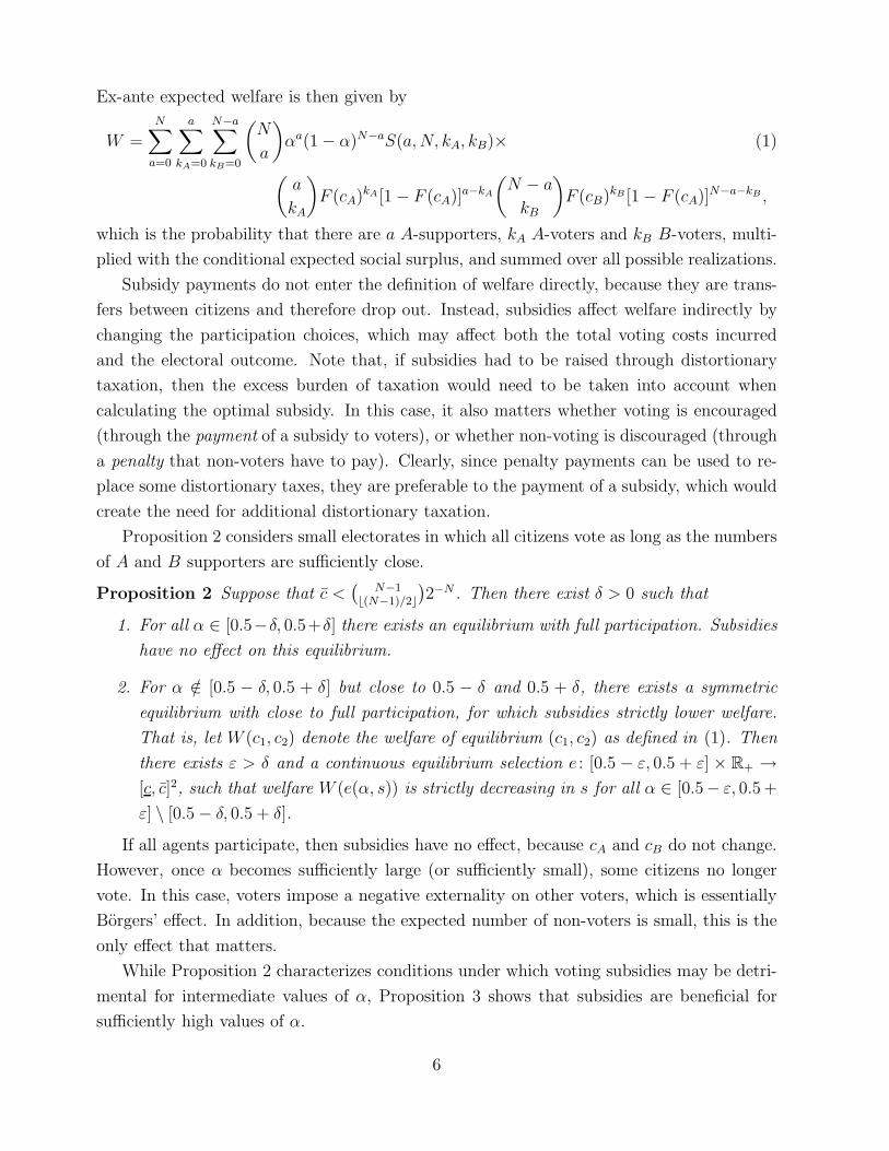
Figure 1: The Marginal Benefit of a Voting Subsidy at s = 0
The results of Propositions 2 and 3 are illustrated in the left panel of Figure 1, which
displays the marginal benefit of a subsidy when voting cost are uniformly distributed in
the interval [0.01, 0.05] and N = 20. For α close to 0.5, all citizens vote voluntarily, so
6Note that citizens with minority preference have a much smaller incentive to free-ride, because the
expected number of other citizens with the same preference is very small.
7
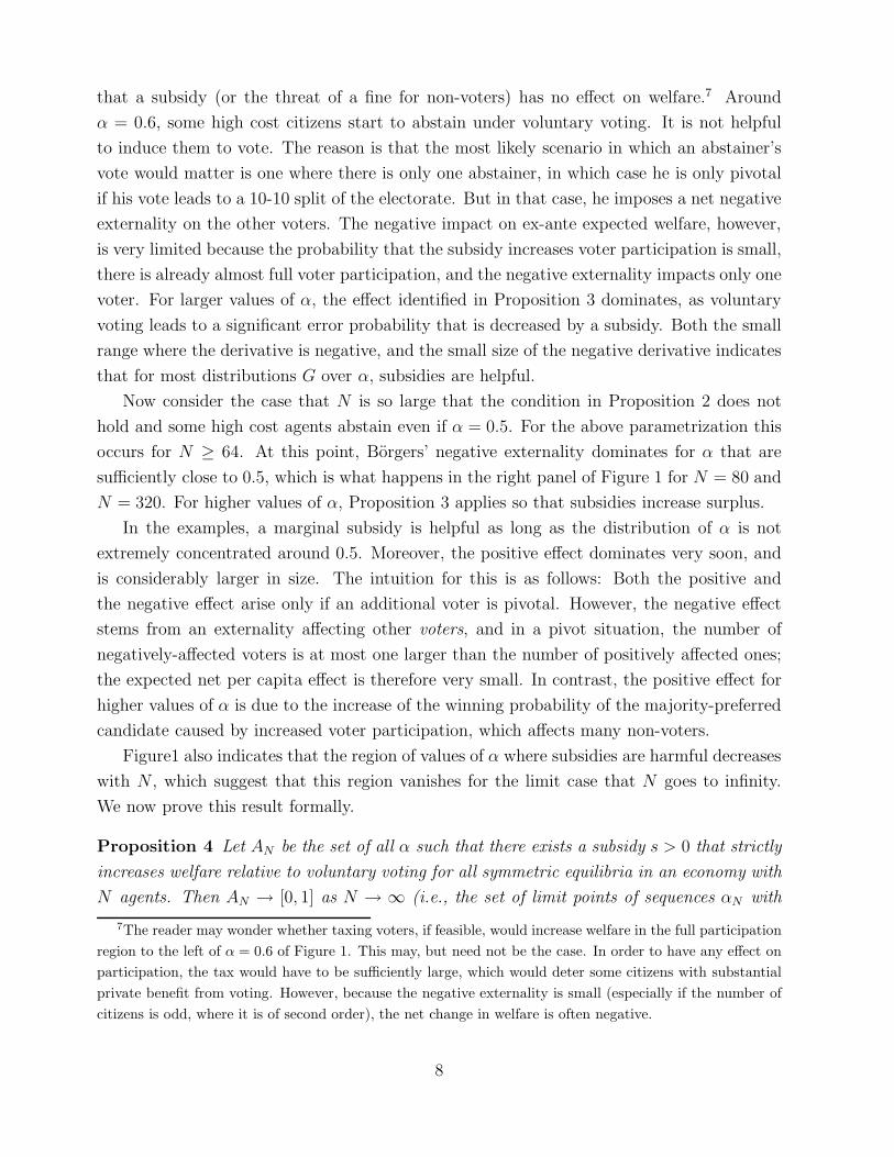
that a subsidy (or the threat of a fine for non-voters) has no effect on welfare.7 Around
α = 0.6, some high cost citizens start to abstain under voluntary voting. It is not helpful
to induce them to vote. The reason is that the most likely scenario in which an abstainer’s
vote would matter is one where there is only one abstainer, in which case he is only pivotal
if his vote leads to a 10-10 split of the electorate. But in that case, he imposes a net negative
externality on the other voters. The negative impact on ex-ante expected welfare, however,
is very limited because the probability that the subsidy increases voter participation is small,
there is already almost full voter participation, and the negative externality impacts only one
voter. For larger values of α, the effect identified in Proposition 3 dominates, as voluntary
voting leads to a significant error probability that is decreased by a subsidy. Both the small
range where the derivative is negative, and the small size of the negative derivative indicates
that for most distributions G over α, subsidies are helpful.
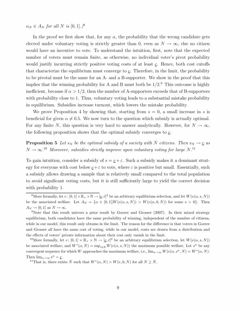
Now consider the case that N is so large that the condition in Proposition 2 does not
hold and some high cost agents abstain even if α = 0.5. For the above parametrization this
occurs for N ≥ 64. At this point, Borgers’ negative externality dominates for α that are
sufficiently close to 0.5, which is what happens in the right panel of Figure 1 for N = 80 and
N = 320. For higher values of α, Proposition 3 applies so that subsidies increase surplus.
In the examples, a marginal subsidy is helpful as long as the distribution of α is not
extremely concentrated around 0.5. Moreover, the positive effect dominates very soon, and
is considerably larger in size. The intuition for this is as follows: Both the positive and
the negative effect arise only if an additional voter is pivotal. However, the negative effect
stems from an externality affecting other voters, and in a pivot situation, the number of
negatively-affected voters is at most one larger than the number of positively affected ones;
the expected net per capita effect is therefore very small. In contrast, the positive effect for
higher values of α is due to the increase of the winning probability of the majority-preferred
candidate caused by increased voter participation, which affects many non-voters.
Figure1 also indicates that the region of values of α where subsidies are harmful decreases
with N , which suggest that this region vanishes for the limit case that N goes to infinity.
We now prove this result formally.
Proposition 4 Let AN be the set of all α such that there exists a subsidy s > 0 that strictly
increases welfare relative to voluntary voting for all symmetric equilibria in an economy with
N agents. Then AN → [0, 1] as N → ∞ (i.e., the set of limit points of sequences αN with
7The reader may wonder whether taxing voters, if feasible, would increase welfare in the full participation
region to the left of α = 0.6 of Figure 1. This may, but need not be the case. In order to have any effect on
participation, the tax would have to be sufficiently large, which would deter some citizens with substantial
private benefit from voting. However, because the negative externality is small (especially if the number of
citizens is odd, where it is of second order), the net change in welfare is often negative.
8
αN ∈ AN for all N is [0, 1].)8
In the proof we first show that, for any α, the probability that the wrong candidate gets
elected under voluntary voting is strictly greater than 0, even as N → ∞, else no citizen
would have an incentive to vote. To understand the intuition, first, note that the expected
number of voters must remain finite, as otherwise, no individual voter’s pivot probability
would justify incurring strictly positive voting costs of at least c. Hence, both cost cutoffs
that characterize the equilibrium must converge to c. Therefore, in the limit, the probability
to be pivotal must be the same for an A- and a B-supporter. We show in the proof that this
implies that the winning probability for A and B must both be 1/2.9 This outcome is highly
inefficient, because if α > 1/2, then the number of A-supporters exceeds that of B-supporters
with probability close to 1. Thus, voluntary voting leads to a substantial mistake probability
in equilibrium. Subsidies increase turnout, which lowers the mistake probability.
We prove Proposition 4 by showing that, starting from s = 0, a small increase in s is
beneficial for given α 6= 0.5. We now turn to the question which subsidy is actually optimal.
For any finite N , this question is very hard to answer analytically. However, for N → ∞,
the following proposition shows that the optimal subsidy converges to c.
Proposition 5 Let sN be the optimal subsidy of a society with N citizens. Then sN → c as
N → ∞.10 Moreover, subsidies strictly improve upon voluntary voting for large N .11
To gain intuition, consider a subsidy of s = c+ ε. Such a subsidy makes it a dominant strat-
egy for everyone with cost below c+ε to vote, where ε is positive but small. Essentially, such
a subsidy allows drawing a sample that is relatively small compared to the total population
to avoid significant voting costs, but it is still sufficiently large to yield the correct decision
with probability 1.
8More formally, let e : [0, 1]×R+×N → [c, c]2 be an arbitrary equilibrium selection, and let W (e(α, s, N))
be the associated welfare. Let AN = {α ∈ [0, 1]|W (e(α, s, N)) > W (e(α, 0, N)) for some s > 0}. Then
AN → [0, 1] as N → ∞.9Note that this result mirrors a prior result by Goeree and Grosser (2007). In their mixed strategy
equilibrium, both candidates have the same probability of winning, independent of the number of citizens,
while in our model, this result only obtains in the limit. The reason for the difference is that voters in Goeree
and Grosser all have the same cost of voting, while in our model, costs are drawn from a distribution and
the effects of voters’ private information about their cost only vanish in the limit.10More formally, let e : [0, 1] × R+ × N → [c, c]2 be an arbitrary equilibrium selection, let W (e(α, s, N))
be associated welfare, and W ∗(α, N) = sups∈RW (e(α, s, N)) the maximum possible welfare. Let sn be any
convergent sequence for which W approaches the maximum welfare, i.e., limn→∞ W (e(α, sn, N) = W ∗(α, N).
Then limn→∞ sn = c.11That is, there exists N such that W ∗(α, N) > W (e, 0, N) for all N ≥ N .
9
4 Robustness
4.1 Asymmetric voting costs
The result of Proposition 5 that a subsidy of s = c + ε can implement the socially op-
timal decision for negligible voting costs depends crucially on the assumption that both
A-supporters’ and B-supporters’ voting costs are distributed according to the same cost dis-
tribution. Consider what happens if, instead, A-supporters’ costs are distributed according
to cumulative distribution function FA(c), while B-supporters’ costs are distributed accord-
ing to cumulative distribution function FB(c). (The difference may affect both the minimum
and maximum voting cost of each type, ci, ci, as well as the distribution of voting costs
in between those extremes). In fact, such a difference in voting cost distributions could be
very natural if the supporters differ systematically in, say, their opportunity cost of time
(e.g., if the proportion of retired and working age citizens differ among A-supporters and
B-supporters).
Consider first what happens in this generalized model when the number of voters is
large and no subsidy is paid. By arguments analogous to those used in the proofs of the
propositions so far, the pivot probability for an A-supporter must go to 2cA, and the pivot
probability for a B-supporter must go to 2cB. If, say, cA < cB, then this can only be the
case if the probability that A wins is larger than the probability that B wins.12 Note that
the equilibrium winning probability is independent of the percentage of citizens who prefer
A or B.13
For example, suppose that cA = 0.01 and cB = 0.015. Using the logic detailed in the
proof of Proposition 3, we can set the right-hand side of (31) equal to 2cA = 0.02, and the
right-hand side of (32) equal to 2cB = 0.03, and solve for vA = 17.1213, vB = 7.5405. (Here,
vi is the expected number of voters for i. The number of voters for candidate i is Poisson
distributed with vi as the parameter of this distribution.) This implies that the probability
that candidate A wins is approximately 0.975.
Now, consider the effect of a subsidy. It is clear that a subsidy of, say, 0.07 would
induce only those A-supporters with voting costs between 0.05 and 0.07 to vote. In this
case, candidate A would win with certainty. Whether this is beneficial or detrimental for
social welfare depends on whether the A-supporters form a majority of the electorate (i.e.,
α > 1/2), and, of course, on the size of voting costs incurred because of the subsidy.
12To see this, note that the pivot probability for a B-supporter is larger than the pivot probability for
an A-supporter if and only if the probability that there is one more A- than B-supporter is larger than
the probability that there is one more B- than A-supporter. This will only be the case if the (Poisson)
distribution of the number of A-supporters dominates the distribution of the number of B-supporters.13The result that the equilibrium winning probability is independent of the preference distribution also
obtains in the model of Campbell (1999) described in the introduction.
10
Let c∗ be the smallest value of c such that FA(c) = FB(c) > 0. That is, c∗ is either
the lowest point at which the two cumulative distribution functions intersect, or, if there is
no such point, then c∗ = max(cA, cB). Setting the subsidy equal to s = c∗ guarantees that
the candidate who is supported by a majority of voters wins the election, because the same
proportion FA(c∗) = FB(c∗) of A-supporters and B-supporters will choose to vote: Clearly,
all voters with c ≤ c∗ have a dominant strategy to vote, and given that infinitely many voters
vote, the pivot probability is equal to zero, so that no voters with higher cost will vote.
Moreover, it is clear that s = c∗ is the cheapest way to guarantee a victory of the majority-
preferred candidate. A subsidy of s = c∗ need not be the optimal subsidy, as non-trivial
voting costs arise, and there is a trade-off between voting costs and probability of making the
correct decision. Let M(s) denote the expected gross welfare from the election outcome given
a subsidy level s, i.e. M(s) =∫ 1
0[αProb(A wins|α, s) + (1 − α)Prob(B wins|α, s)] g(α) dα.
(Note that there is a unique symmetric equilibrium in which voters vote if and only if their
cost parameter is not larger than s, so M(s) is well defined.) Expected net welfare as a
function of s is gross welfare minus aggregate voting cost, i.e.
W (s) = M(s) −∫
αg(α) dα
∫ s
0
cfA(c) dc −(
1 −∫
αg(α) dα
)∫ s
0
cfB(c) dc.
Clearly, the second and third terms are increasing in s, as a higher subsidy will increase
turnout and therefore aggregate voting costs. Since M(·) is maximized at c∗, it is clear that
the optimal subsidy level that maximizes W (·) is strictly less than c∗.
Intuitively, starting from a full participation subsidy, consider lowering the subsidy
slightly, and suppose that this leads to a higher percentage of A-supporters than B-supporters
participating. This leads to some mistakes, that is, victories of candidate A even if α is
slightly below 1/2, but the extent of the mistake is also very small in these cases (because
the A-supporter minority is almost as large as the B-supporter majority). Thus, the welfare
loss from making the wrong decision is a second order effect. In contrast, the cost saving from
some high-cost B-supporters not participating is a first-order effect. Note, however, that the
optimal subsidy can be very close to c∗, and thus (if the cumulative cost distributions of the
two types do not intersect), the optimal policy may be close to compulsory voting, i.e. a
subsidy (or penalty) sufficient to induce almost all citizens to vote in equilibrium.
Suppose, for example, that the voting costs of A-supporters are uniformly distributed
on [0.01, 0.02] and those of B-supporters are uniform on [0.015, 0.025]. Furthermore, let α
be distributed uniformly on [0.4, 0.6]. Without subsidies, or with subsidies below 0.01, the
probability that A wins is independent of the realized α and thus (integrating over α and
taking into account the symmetry of the α−distribution), it is easy to see that the average
expected utility is 0.5.
A somewhat larger subsidy now clearly diminishes welfare: A positive proportion of
11
A-supporters will vote, and candidate A wins with certainty. Given the symmetry of the
distribution of α, this does not increase the average gross payoff of voters from the winning
candidate, and causes an increase in voting costs incurred.
If s > 0.02, all A-supporters vote (so that A receives the votes from a fraction α of
citizens), and the proportion of the population voting for B is (1 − α) s−0.0150.01
. Thus, solving
for α, candidate A will win whenever α ≥ s−0.015s−0.005
. (This implies that the minimum subsidy
such that B can win satisfies s−0.015s−0.005
= 0.4, which can be solved for s = 0.02166). Thus,
W (s) =1
0.6 − 0.4
[
∫ s−0.015
s−0.005
0.4
(1 − α) dα +
∫ 0.6
s−0.015
s−0.005
α dα
]
− 1
20.015 − 1
2
∫ s
0.015
c1
0.6 − 0.4dc
Differentiating with respect to s and solving for s yields that the optimal subsidy in this
case is approximately s = 0.0248, leading to a 98% participation rate of B-supporters (as
well as, of course, a 100% participation of A-supporters). This example therefore shows
that the optimal subsidy (or penalty for not voting) need not be small when the voting cost
distributions of the two types differ, and may have a substantial rather than marginal impact
on the participation rate.
4.2 Subsidies in different models of participation
We have shown that subsidizing participation is typically optimal in our costly voting model.
In this section, we show that this result extends to other models of endogenous participation
in elections. The empirical evidence on the general class of costly voting models (i.e., not
just our version of it) is mixed. On the one hand, the costly voting model predicts that
the minority supporters are more active in equilibrium which makes up for their smaller
numbers (underdog effect). Also, in the costly voting framework, higher participation rates
are expected in close elections (competition effect).14 These comparative static results are
supported by most empirical studies.15
14The terms “underdog effect” and “competition effect” are coined by Levine and Palfrey (2007), who
provide evidence from laboratory experiments for both effects. In our model, the underdog effect (for a large
electorate) is an obvious consequence of the fact that the expected number of votes for A and B must be
approximately equal: If α > 1/2, this can only be the case if B-supporters vote, on average, more often than
A-supporters.
In our framework, the competition effect means that, the closer α is to 1/2, the higher is the expected
equilibrium participation rate. We do not provide a formal result along these lines, and neither do Levine
and Palfrey (2007) in their setup, nor any other paper that we know of. However, the competition effect
holds in all of our numerical examples, as well as in those examples that Levine and Palfrey analyze.15See Matsusaka and Palda (1993), Table 1, for a summary of empirical papers analyzing the relation
between closeness of elections and participation rates. For example, in 35 of 49 regressions reviewed (in
various papers), the margin of victory was a significant predictor of participation rates.
12
On the other hand, the simple costly voting model predicts that participation rates go to
zero for large elections, which is evidently not the case. It is therefore important to analyze
whether voting subsidies may still play an important role in models that can account for
positive equilibrium participation rates in large elections. We first consider a model in which
some voters enjoy voting and show that this gives rise to a new effect that may make subsidies
beneficial. We then sketch how to extend that model to allow for endogenous participation
decisions by leaders that can motivate some voters with positive voting costs to participate.
Consider first a very simple model with an infinite number of citizens. Proportion δ of
the population has zero or negative voting costs (group D – dutiful voters), while proportion
1 − δ has positive voting costs distributed on [c, c] as in our base model (group C – costly
voters). Furthermore, let αD (αC) be the probability a group D (group C) individual prefers
candidate A. From an ex-ante point of view, g(αC , αD) is the density from which αC and αD
are drawn.
Clearly, if there are no subsidies, only citizens who enjoy voting (i.e., who belong to group
D) vote. Therefore, candidate A wins the election if and only if αD > 1/2. From a social
point of view, candidate A should win if and only if α ≡ δαD + (1 − δ)αC > 1/2. Hence,
even if a significant group of individuals have negative voting costs, voluntary participation
guarantees that the correct candidate wins only for a very small class of distributions that
have the property that αD > 1/2 (< 1/2) implies that α > 1/2 (α < 1/2) with probability
1. More generally, the equilibrium per-capita utility under voluntary voting is∫ 1
0
[
∫ 1
1/2[δαD + (1 − δ)αC ] g(αC , αD) dαD +
∫ 1/2
0[1 − δαD − (1 − δ)αC ] g(αC , αD) dαD
]
dαC+δEB,
(2)
where EB is the average benefit that voters in group D receive from voting. Clearly, paying
a subsidy of only c does not significantly increase participation and hence is unlikely to
change the outcome of the election, but paying a subsidy of c (equivalently, compulsory
voting) yields a per-capita utility of∫ 1
0
∫ 1
0
max {δαD + (1 − δ)αC , 1 − δαD − (1 − δ)αC} g(αC , αD) dαD dαC +δEB−(1−δ)EC,
(3)
where EC is the expected per-capita voting cost among voters with positive voting costs.
Since the integral terms in (3) are generically larger than the corresponding terms in (2),
compulsory voting leads to a higher welfare, provided that the average voting cost EC of
the costly voters is sufficiently small.
Note that the model so far can “explain” positive participation rates by assuming that
some people enjoy voting, but it cannot explain the underdog effect and the competition
effect.16 Both effects are well documented, both for large scale elections (see, e.g., Blais
16In an infinitely large electorate, a citizen will vote if and only if his cost of voting is non-positive, because
13
(2000), Shachar and Nalebuff (1999)) and in laboratory experiments (see Levine and Palfrey
(2007)). Alternative endogenous participation models also generate these effects. For exam-
ple, Feddersen and Sandroni (2006) develop a model of ethical voters who receive a moral
benefit that possibly offsets their voting costs, if they feel that they “should” vote. The
ethical rule that specifies the voting cost threshold below which an individual voter “should”
vote is derived endogenously, taking into account both cost considerations and the preference
group’s chance of winning. While no voter is individually pivotal with positive probability
in the model of Feddersen and Sandroni, a positive percentage of ethical voters participates
in the election. Moreover, there is a positive probability that the minority candidate wins,
and ethical minority voters are more likely to participate in equilibrium.
Shachar and Nalebuff (1999) and Herrera and Martinelli (2006) develop models with a
number of “leaders” who favor either candidate A or candidate B and can decide whether to
take a costly action that mobilizes a (random) number of voters to vote for their respective
preferred candidate. Equilibria in these models also feature positive participation rates, a
positive mistake probability and the underdog effect.
We now sketch an extension of the above model that corrects this shortcoming of the
costly voting model. Suppose there are LA “A-leaders” and LB “B-leaders,” who each have
influence over a set of measure ℓ of costly voters who support A and B, respectively. Clearly,
LAℓ ≤ αC and LBℓ ≤ 1 − αC . A leader can “mobilize” his followers by imposing (through
moral pressure etc.) a cost of not voting. Without loss of generality, we can assume that
all his followers vote if a leader mobilizes (otherwise, we can just decrease ℓ accordingly). A
leader’s objective function is a weighted average between utility from the election outcome
and the average voting costs of his followers.17 Also assume that the weight on voting costs
is sufficiently small, so that a leader who knows that he can change the election outcome
by mobilizing would strictly prefer to do so. Candidate A wins the election if and only if
δαD + (1− δ)ℓMA > δ(1−αD) + (1− δ)ℓMB, where MA and MB are the number of A– and
B–leaders who mobilize, respectively. Rearranging this condition, we get
MA − MB >δ
1 − δ
1 − 2αD
ℓ≡ K. (4)
If the expression K on the right hand side of (4) is positive, then it is the critical number by
which the number of mobilizing A–leaders must exceed the number of mobilizing B-leaders
in order for Candidate A to win.
the probability of being pivotal for the election outcome is zero. Note that this would even be true in large
finite electorates: As soon as the expected pivot probability drops below 2c (because of the many voters
with negative participation costs), no voter with voting costs greater or equal to c would participate.17An alternative possibility that leads to qualitatively the same results is that leaders do not care about
their followers’ voting costs, but face some mobilization costs.
14
A leader’s strategic calculations are very similar to the calculations of a costly voter in
our basic model. Provided that δ is not too large (so that costly voters can, in principle,
swing the election to the candidate who is not preferred by the majority of the dutiful vot-
ers), both candidates have a strictly positive chance of winning in equilibrium. If, instead,
δ is large (how large depends also on the value of αD), then only dutiful voters participate
in the election and the majority among them is decisive. This model therefore can explain
the fact that in presidential elections in Utah and Massachusetts, the Republican or Demo-
cratic candidate, respectively, consistently wins: The advantage of one party over the other
among dutiful voters is just so large that leaders do not try to mobilize costly voters and
consequently, the larger preference group wins always. In contrast, the simple costly voting
model (with all voters having voting costs) would predict that Democratic and Republi-
can presidential candidates should each have a significant probability of winning Utah or
Massachusetts.
The effect of leaders on welfare relative to a model in which only dutiful voters vote can
be ambiguous. On the one hand, if the majority group among dutiful voters is not equal to
the majority preference group in the total population, then the presence of leaders makes
it at least possible that the majority-preferred candidate wins. On the other hand, if the
majority group among dutiful voters is equal to the majority preference group in the total
population, then the presence of leaders introduces the possibility that the wrong candidate
wins.
As in the basic model and the voluntary voting model above, it is quite conceivable that
voting subsidies are desirable from a social point of view. With voting subsidies, more costly
voters choose to vote, regardless of the actions of leaders. If the voting subsidy is sufficiently
large to induce most citizens to vote, then the voting outcome is correct decision from a social
perspective. If the average voting cost of costly voters is sufficiently small relative to the
importance of the electoral decision, then subsidies are welfare enhancing in this framework.
5 Conclusion
A central theme in many texts by political scientists dealing with participation in elections
(as well as in newspaper editorials) is that electoral turnout is “too low”. In this paper, we
provide a theoretical framework for this idea. We show that costly voting induces suboptimal
equilibrium participation and frequently leads to wrong choices. We prove that in such a
world, providing incentives for citizens to vote increases the quality of electoral decisions and
social welfare.
Our setup is the simplest model in which questions of costly voting can be studied:
Citizens know which candidate they prefer, they only have to decide whether or not to vote,
15
and the voting costs are drawn from the same distribution for both A and B supporters.
Extending our model to allow for incomplete information about candidates and differential
voting costs for A and B supporters should reinforce our qualitative finding that voting is
similar to providing a public good.
Following much of the literature, we assume that each voter’s benefit from the election
of his preferred candidate is normalized to one, while costs are random draws for individual
voters. More generally, one could assume that each voter’s benefit is also random. However,
if both costs and benefits are drawn from the same distribution for A and B-supporters, the
analysis for voluntary and compulsory voting is largely unchanged.
16
6 Appendix
Proof of Proposition 1. Let cA be given. We construct cB such that an individual who
prefers B is indifferent between voting and not voting if ci = cB.
Consider a supporter of B. The probability that a of the remaining N − 1 individuals
support candidate A and that k of these A supporters participate in the election, is given by
Prob{#A-supporters = a, #A-voters = k} =
(
N − 1
a
)
αa(1−α)N−1−a
(
a
k
)
F (cA)k(1−F (cA))a−k.
(5)
If there are a supporters of A, of whom k participate in the election then our B supporter’s
expected benefit of voting including subsidy s but excluding voting costs is
Benefit(a, k) = 0.5
[(
N − a − 1
k − 1
)
F (cB)k−1(1 − F (cB))N−a−k
+
(
N − a − 1
k
)
F (cB)k(1 − F (cB))N−a−k−1
]
+ s.
(6)
It follows immediately that Prob{#A = a, #A-voters = k} and Benefit(a, k) are continuous
in cA. The expected benefit from voting for a B-supporter with voting costs cB is
EBB(cA, cB) =N−1∑
a=0
a∑
k=0
Prob{#A = a, #A-voters = k}Benefit(a, k), (7)
which is continuous in cA and cB. Similarly, an A-supporter’s gross benefit, EBA(cA, cB), is
continuous. We now define the function T : [c, c]2 → [c, c]2 by
T (cA, cB) =(
max{
min{EBA(cA, cB), c}, c}
, max{
min{EBB(cA, cB), c}, c}
)
.
Clearly, T is continuous. Brouwer’s fixed point theorem therefore implies that there exist
c∗A, c∗B with T (cA, c∗B) = (c∗A, c∗B). Consider c∗A. If c < c∗A < c then the gross benefit of an A
supporter with costs c∗A who participates in the election is exactly c∗A. As a consequence an
A supporter with cost c∗A is indifferent between voting and not voting, and every A supporter
with a lower cost will strictly prefer to vote. Now let c∗A = c. Then EBA(cA, cB) ≤ c. Thus,
no A supporter will will participate, because the probability that c = c is 0. Finally, c∗A = c
implies that all A supporters participate in the voting. Therefore, c∗A is the cost cutoff for A
supporters. Similarly, it follows that c∗B is the equilibrium cutoff for B supporters.
Proof of Proposition 2. First, suppose that N is odd. Consider one particular agent,
and suppose that all remaining agents vote. Then the pivot probability for that agent is
17
given by(
N−1(N−1)/2
)
α(N−1)/2(1−α)(N−1)/2. If the agent is pivotal, then his benefit is 0.5. Thus,
cA = c if and only if
c ≤ 0.5
(
N − 1
(N − 1)/2
)
α(N−1)/2(1 − α)(N−1)/2. (8)
Choose α > 0.5 such that (8) holds with equality. Then δ = α−0.5. If α < α there is already
full participation and subsides are irrelevant. It remains to show that welfare is decreasing
if subsidies are introduced for any α > α that is close to α.
We first show that cA and cB are continuous in α around α. We use the implicit function
theorem, as generalized by Clarke (1983) to non-smooth functions (since F (·) is not contin-
uously differentiable at c).18 Because (1 − F (cA)) = (1 − F (cB)) = 0 at α, we can ignore
terms with (1− F (cA))k or (1− F (cB))k for k ≥ 2, because their derivatives with respect to
cA or cB are zero. Omitting these terms, (7) implies that the benefit of a B supporter from
voting is given by
0.5
[
(
N − 1N−1
2
)
αN−1
2 (1 − α)N−1
2 F (cA)N−1
2
[
N − 1
2F (cB)
N−3
2 (1 − F (cB)) + F (cB)N−1
2
]
+
(
N − 1N+1
2
)
αN+1
2 (1 − α)N−3
2
N + 1
2F (cA)
N−1
2 (1 − F (cA))F (cB)N−3
2
]
− cB.
(9)
If we take derivatives from the right then ∂F (cA)∂cA
|cA≥c = ∂F (cB)∂cB
|cB≥c = 0. Thus,
∂EBA(cA, cB)
∂cA|cA,cB≥c = −1,
∂EBA(cA, cB)
∂cB|cA,cB≥c = 0;
∂EBB(cA, cB)
∂cA
|cA,cB≥c = 0,∂EBB(cA, cB)
∂cB
|cA,cB≥c = −1.
If we take derivatives from the left then
∂EBB(cA, cB)
∂cA
|cA=c,cB≥c = 0.5f(c)N − 1
2
(
N − 1N−1
2
)
αN−1
2 (1 − α)N−3
2 (1 − 2α),
∂EBB(cA, cB)
∂cB
|cA≥c,cB=c = −1.
(10)
By symmetry, the derivatives for A supporters are
∂EBA(cA, cB)
∂cA
|cA=c,cB≥c = −1,
∂EBA(cA, cB)
∂cB
|cA≥c,cB=c = −0.5f(c)N − 1
2
(
N − 1N−1
2
)
αN−3
2 (1 − α)N−1
2 (1 − 2α)(11)
18Theorem 7.1.1 of Clarke (1983) (earlier proved in Clarke (1976)) establishes the inverse function theorem
for Lipschitzian functions, and the subsequent (unnumbered) corollary proves the implicit function theorem.
Note that the uniqueness of the implicit function, which is not explicitly stated in the corollary, follows
immediately from Theorem 7.1.1.
18
Thus, the determinant of right-hand derivatives is strictly positive. Similarly, it follows that
the matrix of derivatives has full rank for any combination of left and right derivatives, which
implies that cA and cB are continuous functions of α.
Consider α that is marginally greater than α. If all agents participate, then a particular
citizen is pivotal if the number of A- and B-voters is the same among the remaining voters.
If our particular citizen votes for candidate A, then the total benefit of all other A-voters
increases by (N −1)/4, while the benefit to B voters is reduced by exactly the same amount.
A subsidy would turn our citizen from a non-voter to a voter if and only if the private
benefit of the person equals his voting costs, i.e., if the person’s net-benefit from voting is
zero. Thus, if all agents participate, there is no effect on surplus.
Now suppose that one of the remaining agents does not vote. Then a particular A
supporter is pivotal if and only if there are (N − 3)/2 A-voters and (N − 1)/2 B-voters
among the remaining agents. Thus, the net-change in benefit to these voters is −0.5 if our
A supporter participates. As above, if a subsidy would induce our A-supporter to vote, then
the private benefit is zero. Thus, the subsidy would lower surplus.
Note that we can ignore the effects when two or more agents do not participate, because
this event is on the order of (1 − F (cA))2 and (1 − F (cB))2, while the above effect is of the
order (1 − F (cA)) and (1 − F (cB)), and F (cA), F (cB) are close to 1.
The proof for even N is similar. With an even number of agents and full participation in
the election, a particular person person, say an A supporter, is pivotal if there are (N −3)/2
A-supporters and (N − 1)/2 B supporters, which implies a negative externality. Again, all
higher order terms can be ignored.
Proof of Proposition 3. Let α = 1. Then an A-supporter is indifferent between voting
and not voting if
[1 − F (cA)]N−1 1
2= cA − s. (12)
Since the left-hand side is non-increasing in cA and the right-hand side is increasing in cA,
there exists a unique value of cA that satisfies (12). Furthermore, for s < c, this unique
symmetric equilibrium at α = 1 satisfies c < cA < c.
Applying the implicit function theorem yields
dcA
ds=
2
2 + (N − 1)f(cA) [1 − F (cA)]N−2> 0. (13)
Substituting a = N , kB = 0, and α = 1 in (1) yields
W =N
2
(
1 − F (cA))N
+
N∑
kA=1
(
N − kAE[c|c ≤ cA])
(
N
kA
)
F (cA)kA(1 − F (cA))N−kA
= N
[
1 − 1
2(1 − F (cA))N −
∫ cA
c
cf(c) dc
]
.
(14)
19
Taking the derivative of (14) with respect to s and using (12) yields
∂W
∂s|s=0 = f(cA)N(N − 1)cA
dcA
ds> 0, (15)
which proves that subsidies increase welfare at α = 1. Finally, using (12), (13) and the
fact that cA → c for N → ∞, implies that the derivative of per-capita surplus, 1N
∂W∂s
|s=0,
converges to 1 as N → ∞.
Next, we prove that equilibrium is unique in a neighborhood of α = 1 and that the
equilibrium values of cA and cB are continuous in α.
First, consider a sequence indexed by i with αi → 1 as i → ∞, and let ciA, ci
B, be
the corresponding equilibrium cost cutoffs. Then, by compactness, there exist subsequences
that converge to some cost levels cA and cB. Continuity of the expected voting benefits (7)
implies that cA, cB is an equilibrium for α = 1. Because the equilibrium at α = 1 is unique,
it follows that for any neighborhood U of the α = 1 equilibrium (cA, cB), there exists an
α < 1 such that all equilibria for α ≥ α are in U. Using the implicit function theorem we
can then establish uniqueness of equilibria in a neighborhood of α = 1. For α > 1 we define
the expected benefit to be equal to that at α = 1. Because the expected benefit functions
are non-smooth at α = 1, we again use Clarke (1983).
Since we can ignore all terms (1 − F (cB)), (7) implies that at an α = 1 equilibrium
1
2(1 − F (cA))N−1 − cA = 0 (16)
1
2
[
(1 − F (cA))N−1 + (N − 1)F (cA)(1 − F (cA))N−2]
− cB = 0. (17)
The derivative of (16) with respect to cA is −0.5(N−1)f(cA) [(1 − F (cA))]N−2−1 and with re-
spect to cB is 0. The derivatives of (17) from are −0.5(N−1)(N−2)f(cA) [(1 − F (cA))]N−3−1
and −1. Thus, the matrix of derivatives has full rank. Clarke (1983) therefore implies that
there exists a unique equilibrium in a neighborhood of α = 1, with cutoffs cA and cB that
are continuous in α.
Finally, ∂W∂s
|s=0 > 0 in a neighborhood of α = 1, since the derivative of (14) with respect
to α is continuous in cA and cB.
Lemma 1 Suppose that c > 0. Then, in any equilibrium, the expected number of A and
B voters, vA(N) and vB(N), are bounded away from ∞, i.e., there exists an M such that
vA(N), vB(N) ≤ M for all N ∈ N.
Proof of Lemma 1. The strategy of the proof is to show that if the expected number of
voters goes to infinity as N → ∞ then the pivot probabilities go to zero. This provides a
contradiction because the voting costs c are always strictly positive, i.e., c ≥ c > 0.
20
First, however, we show that the pivot probabilities go to zero if the expected number
of voters—conditional on an and bn being the realized number of A and B supporters—
converges to infinity as the size of electorate goes to infinity. To do this, we analyze the limit
distribution of the difference in the number of A and B voters.
Let an and bn be the number of A and B supporters, and let Nn = an + bn be the
number of citizens. Let Y an,bn
i be a random variable that assumes the value 1 if A-supporter
i participates in the election, and is 0 otherwise. Define Zan,bn
i analogously for B supporters.
Care must be taken in applying the central limit theorem, because Y an,bn
i and Zan,bn
i converge
to zero a.e., as an and bn → ∞.19
Claim 1. Let an, bn ∈ N such that limn→∞ anF (cA(an)) = limn→∞ bnF (cB(Nn)) = ∞. where
Nn = an + bn. Furthermore, suppose that lim supn→∞ cA(Nn) < c and lim supn→∞ cB(Nn) <
c. Then
limn→∞
P
∑an
i=1 Y an,bn
i − ∑bn
i=1 Zan,bn
i − anF (cA(Nn)) + bnF (cB(Nn))√
an var[
Y an,bn
i
]
+ bn var[
Zan,bn
i
]
≤ λ
=1√2π
∫ λ
−∞e−
x2
2 dx,
(18)
where the convergence is uniform in λ.
Let Cn =∑an
i=1 E[|Y an,bn
i − F (cA(Nn))|2+δ] +∑bn
i=1 E[|Zan,bn
i − F (cB(Nn))|2+δ], for some
δ > 0. According to Theorem 4.4 in Chapter 4 of Doob (1990) it is sufficient to check that
limn→∞
Cn(
an var[
Y an,bn
i
]
+ bn var[
Zan,bn
i
]
)1+δ/2= 0. (19)
Recall that Y an,bn
i and Zan,bn
i assume the value 1 with probabilities F (cA(Nn)) and F (cB(Nn)),
respectively; and the value 0 otherwise. Thus, var[
Y an,bn
i
]
= F (cA(Nn))(1−F (cA(Nn))) and
19In fact, the distinction between this result and that in Lemma 2 is as follows. Here, we show that if
the expected number of voters were to go to infinity, then the limit distribution would be normal (which, as
shown below, leads to a contradiction). In contrast, the Poisson limit distribution in Lemma 2 is compatible
with strictly positive voting costs.
21
var[
Zan,bn
i
]
= F (cB(Nn))(1 − F (cB(Nn))). Consequently,
limn→∞
Cn(
an var[
Y an,bn
i
]
+ bn var[
Zan,bn
i
]
)1+δ/2
≤ limn→∞
∑an
i=1 E[|Y an,bn
i − F (cA(Nn))|2+δ](
an var[
Y an,bn
i
]]
)1+δ/2+ lim
n→∞
∑bn
i=1 E[|Zan,bn
i − F (cB(Nn))|2+δ](
bn var[
Y bn
i
]])1+δ/2
= limn→∞
anF (cA(Nn))(1 − F (cA(Nn)))[
(1 − F (cA(Nn)))1+δ + F (cA(Nn))1+δ]
[
anF (cA(Nn))(1 − F (cA))]1+δ/2
+ limn→∞
bnF (cB(Nn))(1 − F (cB(Nn)))[
(1 − F (cB(Nn)))1+δ + F (cB(Nn))1+δ]
[
bnF (cB(Nn))(1 − F (cB(Nn)))]1+δ/2
= limn→∞
(1 − F (cA(Nn)))1+δ + F (cA(Nn))1+δ
[
anF (cA(Nn))(1 − F (cA(Nn)))]δ/2
+ limn→∞
(1 − F (cB(Nn)))1+δ + F (cB(Nn))1+δ
[
bnF (cB(Nn))(1 − F (cB(Nn)))]δ/2
= 0,
as, by assumption, limn→∞ anF (cA(Nn)) = limn→∞ bnF (cB(Nn)) = ∞, and lim supn→∞ cA(Nn) <
c and lim supn→∞ cB(Nn) < c. Thus, condition (19) is satisfied, proving claim 1.
Claim 2. Suppose that the assumptions of Claim 1 are satisfied. Let PivA(an, bn) and
PivB(an, bn) the privot probability of an A and B supporter given that the number of A and
B supporters is an and bn. Then
limn→∞
PivA(an, bn) = limn→∞
PivB(an, bn) = 0, (20)
Define
q = limn→∞
anF (cA(Nn)) − bnF (cB(Nn))√
an var[
Y an,bn
i
]
+ bn var[
Zan,bn
i
]
. (21)
Note that we allow for the possibility that q is negative or positive infinity. Furthermore, we
can assume without loss of generality that the sequence converges. Otherwise, we can take
a converging subsequence. Let ε > 0 be arbitrary. Then there exists λ > 0 such that
1√2π
∫ q+λ
q−λ
e−x2
2 dx < ε. (22)
Furthermore,
limn→∞
√
an var[
Y an,bn
i
]
+ bn var[
Zbn
i
]
= ∞. (23)
This follows again because var[
Y an,bn
i
]
= F (cA(Nn))(1 − F (cA(Nn))) and var[
Zan,bn
i
]
=
F (cB(Nn))(1−F (cB(Nn))), and because anF (cA(an)) and bnF (cB(Nn)) converge to ∞ while
(1 − F (cA(Nn))) and (1 − F (cB(Nn))) remain positive.
22
Note that if an agent is pivotal in the election then∑an
i=1 Y an,bn
i −∑bn
i=1 Zan,bn
i ∈ {−1, 0, 1}.Thus, (23), and (21) imply that for sufficiently large n, a necessary condition for being pivotal
is that
q − λ ≤∑an
i=1 Y an,bn
i −∑bn
i=1 Zan,bn
i − anF (cA(Nn)) + bnF (cB(Nn))√
an var[
Y an,bn
i
]
+ bn var[
Zan,bn
i
]
≤ q + λ. (24)
Thus, (22), (24), and claim 1 imply that the probability of being pivotal is less than ε,
proving claim 2.
Suppose, by way of contradiction, that there exists a subsequence of voting games Nn, n ∈N such that limn→∞ vA(Nn) = limn→∞ vB(Nn) = ∞ (the case where the expected number of
one type of voter remains finite is similar and omitted). Then, because the expected number
of A and B voters are given by vA(N) = F (cA(N))αN and vB(N) = F (cB(N))(1 − α)N ,
respectively, we have
limn→∞
F (cA(Nn))Nn = ∞, and limn→∞
F (cB(Nn))Nn = ∞. (25)
The law of large numbers implies that limn→∞ an/N = α and limn→∞ bn/N = (1−α) for a.e.
sequence of realizations an and bn. Furthermore, we can assume that cA(Nn) and cB(Nn)
remain bounded away from c. Otherwise, all agents participate and it is immediate that
the pivot probability converges to zero. Thus, (20) holds a.e. As a consequence, Lebesgue’s
dominated convergence Theorem implies that the (unconditional) pivot probability converges
to zero, a contradiction, since then, each citizen would be better off not voting.
Lemma 2 Suppose that c > 0. Then, in any equilibrium, the probability that candidate A
wins the election under voluntary voting converges to 12
as N → ∞.
Proof of Lemma 2. Lemma 1 implies that there exists a sequence of voting games Nn,
n ∈ N with limn→∞ vA(Nn) = vA and limn→∞ vB(Nn) = vB. Let an and bn be the realized
number of A and B supporters when there are Nn citizens. Then the law of large numbers
implies that limn→∞ an/Nn = α, for a.e. realization of A and B supporters. We first prove
that∑an
i=1 Y an,bn
i and∑bn
i=1 Zan,bn
i converge to Poisson distributions.
The expected number of A voters, given that there are an supporters of A, is vA(Nn|an) =
anF (cA(Nn)). Thus,
(
an
k
)
F (cA(Nn))k(1 − F (cA(Nn)))an−k
=(an − 1) . . . (an − k + 1)
ak−1n
vA(Nn|an)k
k!
(
1 − vA(Nn|an))
an
)an−k
.
(26)
23
Note that
limN→∞
vA(Nn|an)
vA(Nn)= lim
N→∞
anF (cA(Nn))
αNF (cA(Nn))= 1, (27)
because aN/N converges to α. This implies limn→∞ vA(Nn|an) = vA. Thus, (26) and (27)
imply
limn→∞
P({
#A-voters = k}
|{
#A-supporters = an
})
=vk
A
k!e−vA ,
for a.e. sequence of realizations of an. Taking the expectation over all realizations an and
using Lebesgue’s dominated convergence theorem implies
limn→∞
P({
#A-voters = k}
|Nn
)
=vk
A
k!e−vA, (28)
where the convergence is uniform in k. Similarly, limn→∞ P({
#B-voters = k}
|Nn
)
=vk
B
k!e−vB . An A supporter with cost ci votes if and only if
1
2P
(
#A-voters − #B-voters ∈ {0,−1}|Nn
)
≥ ci, (29)
where P (#A-voters − #B-voters ∈ {0,−1}|Nn) is the probability that candidate A gets
either one less vote or the same number of votes as candidate B, given that there are Nn
individuals. Thus, (28) implies
limn→∞
P (#A-voters − #B-voters ∈ {0,−1}|Nn) =
∞∑
i=0
viA
i!e−vA
(
viB
i!e−vB +
vi+1B
(i + 1)!e−vB
)
,
(30)
By formula 9.6.10 in Abramowitz and Stegun (1965) (see also Myerson (2000)), we get
limn→∞
P (#A-voters − #B-voters ∈ {0,−1}|Nn) =
√
vA
vB
(
I1(2√
vAvB)
evA+vB
+I0(2
√vAvB)
evA+vB
)
,
(31)
where Ik is a modified Bessel function. Similarly, the pivot probability for a B supporter is
limn→∞
P (#A-voters − #B-voters ∈ {0, 1}|Nn) =
√
vB
vA
(
I1(2√
vAvB)
evA+vB
+I0(2
√vAvB)
evA+vB
)
. (32)
As n → ∞ both pivot probabilities in (31) and (32) must converge to 2c, by (29) and Lemma
1. Thus,
√
vA
vB
(
I1(2√
vAvB)
evA+vB
+I0(2
√vAvB)
evA+vB
)
=
√
vB
vA
(
I1(2√
vAvB)
evA+vB
+I0(2
√vAvB)
evA+vB
)
. (33)
However, since the Bessel function I1 is never zero, (33) implies that vA = vB, i.e., in the
limit the number of A and B voters are drawn from the same Poisson distribution. As a
24
consequence, each candidate wins with probability 12, independent of α. This proves the
result since the winning probability is independent of the sequence Nn that was chosen.
Proof of Proposition 4. Lemma 2 implies that the wrong candidate is elected with
probability 0.5 as N → ∞. Thus, expected per-capita surplus under voluntary voting
converges to 0.5.
Now consider a subsidy s = c+ ε. Then the number of voters goes to infinity as N → ∞,
because at least all citizens with costs c ≤ c+ε vote. Thus, the pivot probability goes to zero,
which implies that cA, cB → c+ε. As a consequence, if α 6= 0.5, then the majority candidate
wins with probability 1 as N → ∞. Thus, ex-ante expected per-capita surplus converges to
max{α, (1−α)}−∫ c+ε
cc dF (c). Since ε can be chosen arbitrarily, the expected surplus given
the subsidy exceeds the expected surplus from voluntary voting. As a consequence [0, 1] is
the set of limit points of sequences αN ∈ AN .
Proof of Proposition 5. Let SN,s(α) be the ex-ante expected surplus, given N citizens
and a subsidy s. The proof of Proposition 4 implies that limN→∞ SN,S(α) = max{α, (1 −α)} −
∫ c+s
cc dF (c), for a.e. α. Thus, limN→∞
∫
SN,sg(α) dα =∫
max{α, (1 − α)}g(α) dα −∫ c+s
cc dF (c) by Lebesgue’s dominated convergence theorem. If s ↓ c, we can therefore get
arbitrarily close to the first best. In contrast, if s ≥ γ > c, then there remains a loss of at least∫ c+γ
cc dF (c) in the limit. Similarly, if s ≤ γ < c, then Lemma 2 implies a strictly positive
probability that the wrong candidate is elected when N is large, and expected surplus is
again bounded aways from the first best. Thus, sN → c.
25
References
Abramowitz, M. and I. Stegun (1965). Handbook of Mathematical Tables. New York, Dover
Publications.
Blais, A. (2000). To vote or not to vote: The merits and limits of rational choice theory.
University of Pittsburgh Press.
Borgers, T. (2004). Costly voting. American Economic Review 94 (1), 57–66.
Campbell, C. M. (1999). Large electorates and decisive minorities. Journal of Political
Economy 107, 1199–1217.
Clarke, F. (1976). On the inverse function theorem. Pacific Journal of Mathematics 64,
97–102.
Clarke, F. (1983). Optimization and Nonsmooth Analysis. New York, John Wiley & Sons.
Dean, J. (2003). Is it time to consider mandatory voting laws? Findlaw.com. Posted
Friday, Feb. 28, 2003.
Doob, J. (1990). Stochastic Processes. New York, John Wiley & Sons.
Feddersen, T. and A. Sandroni (2006). A theory of participation in elections with ethical
voters. American Economic Review 96, 1271–1282.
Ghosal, S. and B. Lockwood (2004). Costly voting and inefficient participation. University
of Warwick.
Goeree, J. and J. Grosser (2007). Welfare reducing polls. Economic Theory 31, 51–68.
Herrera, H. and C. Martinelli (2006). Group formation and voter participation. Theoretical
Economics 1, 461–487.
Ledyard, J. (1984). Pure theory of two-candidate competition. Public Choice 44, 7–41.
Levine, D. and T. Palfrey (2007). The paradox of voter participation? A laboratory study.
American Political Science Review 101, 143–158.
Matsusaka, J. G. and F. Palda (1993). The downsian voter meets the ecological fallacy.
Public Choice 77, 855–878.
Myerson, R. B. (2000). Large poisson games. Journal of Economic Theory 94, 7–45.
Olbermann, K. (2002). Make voting mandatory! Salon.com. Posted Nov. 5, 2002.
Palfrey, T. R. and H. Rosenthal (1983). A strategic calculus of voting. Public Choice 41,
7–53.
Palfrey, T. R. and H. Rosenthal (1985). Voter participation and strategic uncertainty.
American Political Science Review 79, 62–78.
26

Shachar, R. and B. Nalebuff (1999). Follow the leader: Theory and evidence on political
participation. American Economic Review 89 (3), 525–547.
Taylor, C. R. and H. Yildirim (2006). An analysis of rational voting with private values
and cost uncertainty. Duke University.
Weiner, E. (2004). You must vote. It’s the law. Australia requires citizens to vote. should
the U.S.? Slate. Posted Friday, Oct. 29, 2004.
27


