
Interprocedural Control Dependence
James Ezick and Kiri Wagstaff
CS 612
May 4, 1999
2
Outline
• Motivation• Some essential terms• Constructing the interprocedural postdominance
relation• Answering interprocedural control dependence
queries• Future work
3
Motivation
• As we have seen in class the Roman Chariots formulation for intraprocedural control dependence (Pingali & Bilardi) has allowed control dependence queries to be answered in (optimal) time proportional to the output size.
• We seek to extend that work to cover control flow graphs representing multiple procedures without the need for fully cloning each function.
4
How would that make the world better?
• Recall that control dependence (conds) is the same as the edge dominance frontier relation of the reverse graph.
• Recall that the dominance frontier relation is used in the construction of SSA form representations.
• If we could build this representation faster it would allow us perform a wide range of code optimizations in a more uniform and more efficient manner.

5
Valid Paths - Context Sensitive Analysis
• Valid path: A path from START to END in which call and return edges occur in well-nested pairs and in which these pairs correspond to call sites and the return sites specific to these call sites.
START
a
b
c
d
F
END
This is intended to exactly capture ourintuition of a call stack.

6
Other Terms
• Node w interprocedurally postdominates v if every valid path from v to end contains w.
• Node w is ip control dependent on edge (u v) if– w ip postdominates v
– w does not strictly ip postdominate u
We notice immediately that these definitions are completely analogous to their intraprocedural counterparts - they however incorporate the notionof valid paths.

7
First postdominence, then the world!
As the definitions suggest there is a tight relationship between control dependence and postdominance.
To compute control dependence we first would like to compute postdominance subject to the following criteria:
• We minimize cloning to the fullest possible extent.• We are able to parallelize the process. (One
function - one thread).• We can deal with all common code constructs
(including recursion).

8
Computing Postdominance
• In the intraprocedural case every path through the control flow graph is a valid path and the resulting postdominance relation is a tree.
• Algorithms exist to produce this tree which run in time linear in the size of the control flow graph (Rodgers, et al.).
• The introduction of non-valid paths into the CFG breaks this property - the transitive reduction is now a DAG.
9
How is this done today?
• We use iterative methods and context sensitive flow analysis to compute postdominance and control dependence.
• This involves keeping a table of inputs and outputs.
• Convergence occurs due to the finite nature of the table but it is not guaranteed to occur quickly.

10
General Description
• First, we do a generalized form of dataflow analysis in which each procedure acts as a single block box transition function.
• By keeping a table of inputs and outputs of this function for each procedure we gain efficiency and can detect termination.
• After the interprocedural relationships are understood - we compute the intraprocedural info for each procedure in the usual way.
11
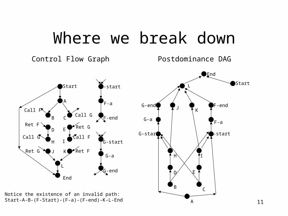
Where we break down
Start
End
F-start
F-a
F-end
G-start
G-a
G-end
A
B C
D E
H I
J K
L
Call F
Call G
Call G
Call F
Ret G
Ret FRet G
Ret F
End
StartL
J K
H
G-start
G-a
G-end F-end
F-a
F-start
I
D E
B C
A
Notice the existence of an invalid path:Start-A-B-(F-Start)-(F-a)-(F-end)-K-L-End
Control Flow Graph Postdominance DAG

12
So What?
• We could ignore the invalid paths and claim that we are being “conservative”.
• However, if we do this we lose the fact that A is postdominated by both F and G - this is vital information that we can’t sacrifice and still expect to be able to compute control dependence.
• We need to construct this DAG in its full form.

13
Observations
• We notice that the postdominance relations for F and G are subgraphs of the entire postdominance relation.
• This begs the question - Can we simply compute the postdominance relation with place-holders for F and G and then simply splice the F and G graphs in later?
• What information would we need to do this?

14
First Attempt
• Is it enough to simply know the two nodes that “bookend” all the calls to a specific function?
Start
End
Call F
Ret F
Call F
Ret F
A
B C
D
E G
H I
Start
End
A
D
B C
E
H
Call FG
I Ret F
Call F
Ret F
End
StartD
B C I
G
H
E
A
We notice that these two distinct control flow graphs produce the same postdominance DAG minus the presence of the F subgraph. Further, [A,D] bookends the calls to F in each case.

15
Defeat!
• Clearly, this technique fails to capture the fact that in the first case the F subgraph should postdominate both B and C whereas in the second case it should not.
• Conclusion: we need to know more than which link to break - we need to know what to do with the ancestors of the destination.
16
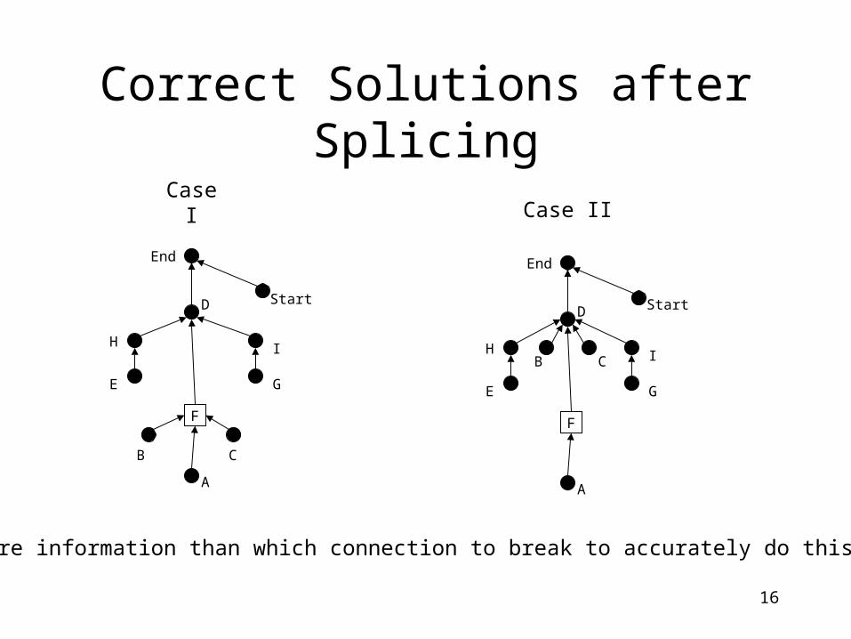
Correct Solutions after Splicing
StartD
B C I
G
H
E
F
A
StartD
C
I
G
H
E
F
A
B
Case I Case II
We need more information than which connection to break to accurately do this splice.
EndEnd
17
What do we need to know?
• We can think of a tree or a DAG as a representation of a partial order. Specifically we can think of the postdominance relation as a partial order since it is reflexive, anti-symmetric and transitive.
• Given this insight, we see that we need to inject the F subgraph into the partial order. Simply knowing two bounds is not enough to do this.

18
It gets worse
• In the example provided we only needed to place B & C - singleton ancestors of D. In fact we can build CFGs where we have arbitrarily complex subgraphs feeding into D.
D
A
FWe want to “splice” F in between D and A.
UVW
X
Y
Z

19
• In order to inject F into the partial order we must also inject F into every path from a terminal to D.
100,100
0,0
F
40,7560,60
70,7050,80
90,90
65,45
We define the partial order as := (a,b) < (c,d) iff (a<c) and (b<d).
100,100
0,0
F
40,7560,60
70,7050,80
90,90
65,45
100,100
0,0
F
40,7560,60
70,70
50,80
90,90
65,45
95,5 95,9572,78
Furthermore, determining where to break each path requires a sequence of UPD queries.
20
Union Postdominance
• We say that a set T union postdominates a set S in an interprocedural control flow graph if every valid path from an element of S to end contains an element of T.
• In the preceding case we must determine for each element of the subtree if it is union postdominated by all of the calls to a specific function.
• This is clearly not promising.• This extends Generalized Dominators (Gupta 92).

21
OK, so we do that - what then?
• Our problems do not end there - consider the following CFG.
Start
End
B C
DE
I
Call F
Ret F
Call G
Ret G
Call H
Ret H
F-Start
F-End
F-A
F-B Call H
Ret H
G-Start
G-End
H-Start
H-End
H-A
Control Flow Graph for Main Control Flow Graph for F Control Flow Graph for G Control Flow Graph for H
G-A
G-C
G-D
G-E
G-B
22
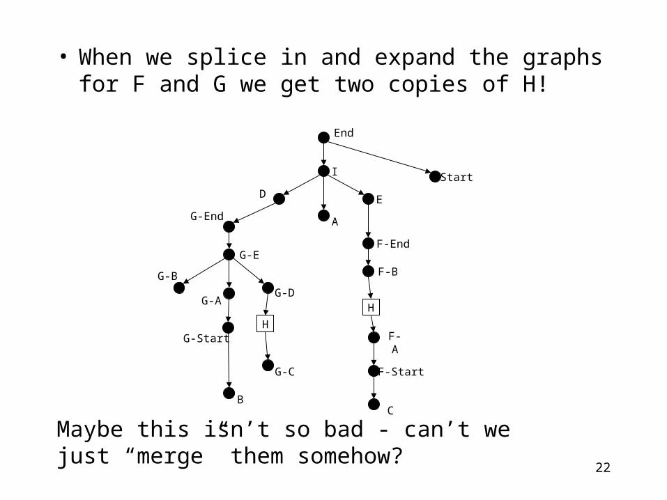
• When we splice in and expand the graphs for F and G we get two copies of H!
H
H
End
Start
E
F-End
F-B
F-A
F-Start
CB
G-C
G-Start
G-D
G-E
G-B
G-End
D
A
I
Maybe this isn’t so bad - can’t we just “merge” them somehow?
G-A
23
Oh, it’s bad.
• Given the partial postdominance relation all I can recover from it about H is that H should be a child of I.
• I don’t know which link from I to break; also I again don’t know what to do with the other children of I.
• As with the previous case I can create CFGs that make this arbitrarily complicated. Further I must now do UPD queries over the entire CFG.

24
Plan “A” is a loser
• It is clear that we cannot simply compute these function DAGs independently and then splice them together since the splicing is more expensive than the original computation.
• We need to find a way to incorporate the splicing information into the original computation.
• In essence we need subgraph “placeholders” for each function.
25
A New Hope
• It is clear that in order to construct the postdominator relation componentwise we need more a priori information.
• In essence we need to understand all of the possible call sequences a program segment can initiate - then we let transitivity do the rest.
• To that end we introduce the notion of “sparse stubs”.

26
Sparse Stubs
• Given a program for which we want to construct a control flow graph we construct a sparse representation in parallel that captures only calls and branches.
• We then use this sparse representation as a “stub” which we inject into the gap between a call and return.
• This stub then captures what we need to construct a PDD into which we can inject full subgraphs.

27
An Example
HH
Start
End
F-Start
F-End
G-Start
G-End
Sparse Representation
Notice that this captures every possible sequence of calls in the program (starts and ends).
Since H is a “terminal function” we can represent it as a singleton. F, G (which are not terminal) cannot be represented this way - else we could not distinguish between “F calls H” and “call F then H”.
We can employ similar shortcuts to eliminate “repeated suffixes” (ex. “call F, call G, call F”)In the case of recursion the sparse graph will have a loop from the call back to the start node of the function - but that’s fine.

28
That’s great. What now?
• We notice immediately some interesting properties of this sparse graph. First any function that is called multiple times will have multiple representations in this graph - but they are all the same. Build them once and use pointers.
• If we inject into the “call gap” of a function the subgraph of the sparse representation between start and end we get a “plug” for the gap.

29
What about this plug?
• We notice that the plug captures exactly all of the valid paths of the program.
• Further, it contains enough information to produce in the resulting PDD placeholders for the component functions.
• The price of this good fortune is that we now have duplicate nodes in the control flow graph (these however are all start & end nodes).

30
Union Postdominance
• We now have a purely graph theoretic problem for which we need (have?) a good algorithm.
• Given a directed graph with a source and sink and a partition of the nodes P - construct the PDD consisting of the elements of the partition.
• We have a naïve quadratic algorithm to do this but we are looking at existing algorithms with better performance that solve similar problems.
31
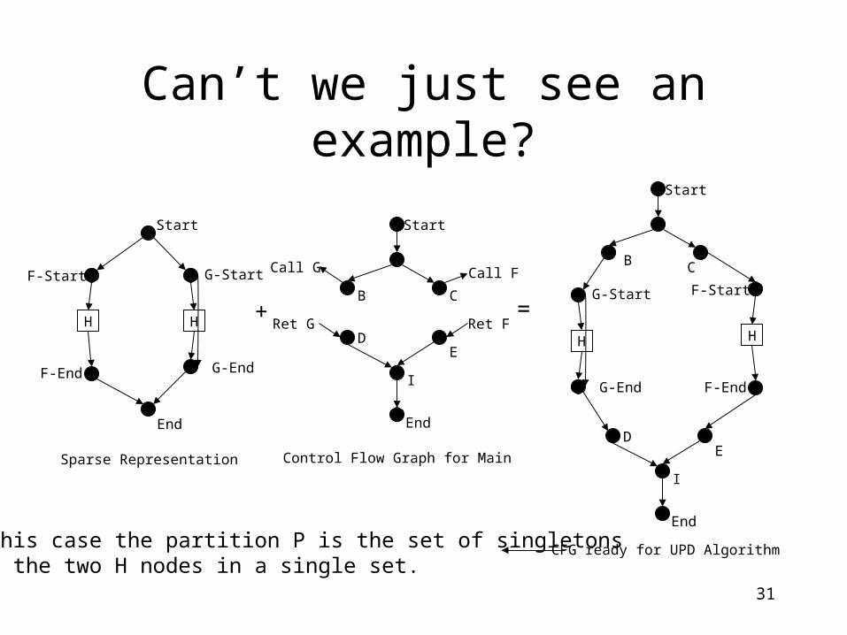
Can’t we just see an example?
HH
Start
End
F-Start
F-End
G-Start
G-End
Sparse Representation
Start
End
B C
DE
I
Call F
Ret F
Call G
Ret G+ =
Control Flow Graph for Main
Start
End
B C
DE
I
H
F-Start
F-End
H
G-Start
G-End
CFG ready for UPD AlgorithmIn this case the partition P is the set of singletonswith the two H nodes in a single set.
32
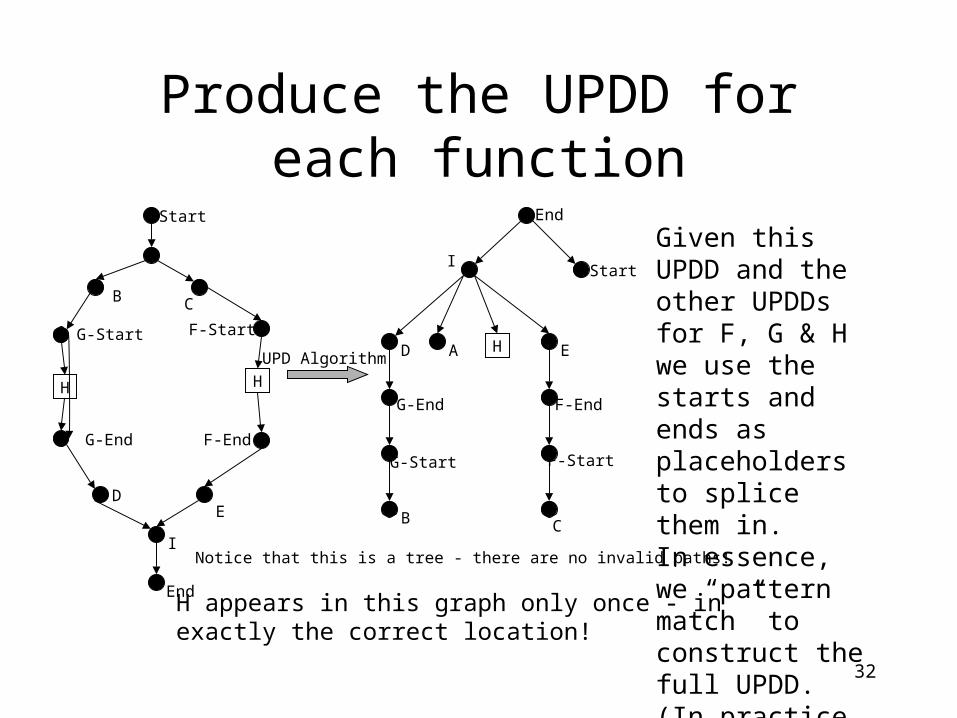
Produce the UPDD for each function
Start
End
B C
DE
I
H
F-Start
F-End
H
G-Start
G-End
H
Notice that this is a tree - there are no invalid paths!
End
Start
B C
G-Start
G-End
F-Start
F-End
A
I
ED
H appears in this graph only once - in exactly the correct location!
UPD Algorithm
Given this UPDD and the other UPDDs for F, G & H we use the starts and ends as placeholders to splice them in.In essence, we “pattern match” to construct the full UPDD. (In practice - use pointers.)

33
Final Observations
• We notice that the only cloning which has occurred related to the functions called - not their functionality
• Once the sparse stub graph is constructed the individual UPDD can be constructed independently.
• Using pointers - splicing is now constant time.• We can deal with recursion and cyclic calls.
34
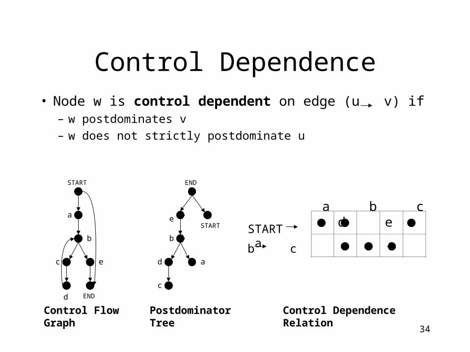
Control Dependence
• Node w is control dependent on edge (u v) if– w postdominates v
– w does not strictly postdominate u
Control Flow Graph Postdominator Tree
START
a
b
c e
d END
END
d
e
c
b
a
START
a b c d e
Control Dependence Relation
START a
b c

35
Queries on Control Dependence
• cd(e): set of nodes control dependent on edge e
• conds(v): set of edges v is control dependent on
• cdequiv(v): set of nodes with same control dependencies as node v
a b c d e
Control Dependence Relation
START a
b c

36
Roman Chariots: cd(e)• Represent cd(e) as an interval on the pdom tree• cd(u v) = [v, END] - [u, END] = [v, parent(u))
– cd(START a) = [a, END)– cd(b c) = [c, e)
a b c d e
Control Dependence Relation
START a
b c
Postdominator Tree
END
d
e
c
b
a
START
a
37
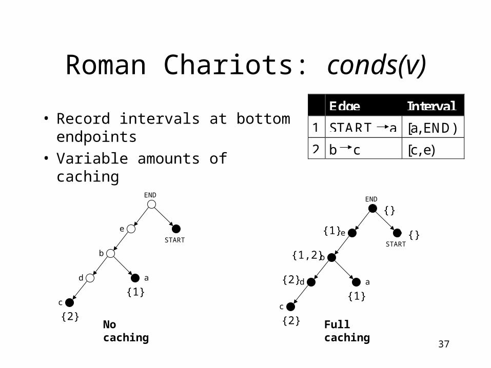
Roman Chariots: conds(v)
• Record intervals at bottom endpoints
• Variable amounts of caching
No caching
END
d
e
c
b
a a
Full caching
END
d
e
c
b
a a{1}
STARTSTART
{2} {2}
{2}
{1}
{1,2}
{1}
{}
{}
Edge Interval
1 START a [a, END)
2 b c [c, e)

38
Vertex conds(v) Size Lo
a {1} 1 a
b {1,2} 2 b
e {1} 1 a
Roman Chariots: cdequiv(v)
• Compute fingerprints for conds sets– size of conds set
– lo(conds): lowest node contained in all intervals in conds set
• Two conds sets are equal iff fingerprints matchIntervals
1 START a [a, END)
2 b c [c, e)
39
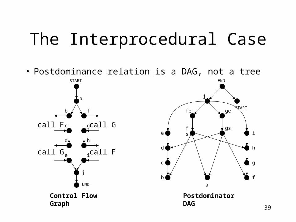
The Interprocedural Case
• Postdominance relation is a DAG, not a tree
Control Flow Graph Postdominator DAG
START
a
b f
j
END
END
ge
j
fe
i
START
c
d
g
h
ie call F
call Gcall F
call Gh
g
f
a
gsfse
d
c
b
40
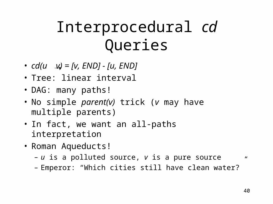
Interprocedural cd Queries
• cd(u v) = [v, END] - [u, END]
• Tree: linear interval
• DAG: many paths!
• No simple parent(v) trick (v may have multiple parents)
• In fact, we want an all-paths interpretation
• Roman Aqueducts!– u is a polluted source, v is a pure source
– Emperor: “Which cities still have clean water?”
41
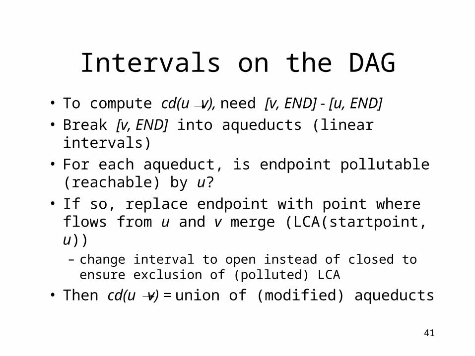
Intervals on the DAG
• To compute cd(u v), need [v, END] - [u, END]• Break [v, END] into aqueducts (linear intervals)• For each aqueduct, is endpoint pollutable
(reachable) by u?• If so, replace endpoint with point where flows
from u and v merge (LCA(startpoint, u))– change interval to open instead of closed to ensure
exclusion of (polluted) LCA
• Then cd(u v) = union of (modified) aqueducts

42
Example: cd(a b)
cd(a b)
= [b,b] + [c,d] + [fs,fs) +
[e, j) +[gs,gs)
= {b,c,d,e}Postdominator DAG
END
ge
j
fe
i
START
h
g
f
a
gsfse
d
c
b
Aqueduct Reachablefrom a?
LCA(startpoint,a)
ModifiedAqueduct
[b, b] N - [b, b]
[c, d] N - [c, d]
[fs, END] Y fs [fs, fs)
[e, END] Y j [e, j)
[gs, END] Y gs [gs, gs)

43
Interprocedural conds Queries
• Emperor: “Which flows pass through a certain city?”
• Search all aqueduct systems for that city
• Faster: use variable caching
Postdominator DAG
END
ge
j
fe
i
START
h
g
f
a
gsfse
d
c
b
Edge Aqueduct System
1 START a {a,fs,fe,gs,ge,j}
2 a b {b,c,d,e}
3 a f {f,g,h,i}
44
Interprocedural cdequiv Queries
• Emperor: “I know that one city is polluted. What other cities are similarly affected?”
• Compare aqueduct systems for all cities for matches
• Faster: apply ‘fingerprint’ approach

45
Final Observations II
• We can compute intervals on the DAG (viewed as Roman Aqueducts)
• We have shown procedures for answering interprocedural control dependence queries
• We may be able to extend the faster methods from the Roman Chariots approach to the interprocedural case as well

46
In Conclusion ...
• We have demonstrated a foundation on which to build an interprocedural analysis capable of dealing with modern programming constructs without resorting to iteration or extensive cloning.
• What lies ahead is to prove this foundation correct and superior to existing techniques with more rigorous proofs and a working implementation.
• At this time we are very optimistic about this formulation.


