
Interactive Mapping Using Range Sensor Data
under Localization Uncertainty
Pedro Goncalo Soares Vieira
Dissertation submitted for obtaining the degree of
Master in Electrical and Computer Engineering
Examination Committee
Chairperson: Prof. Carlos Filipe Gomes BispoSupervisor: Prof. Rodrigo Martins de Matos VenturaMember of the committee: Prof. Carlos Antonio Roque Martinho
December 2012


There are two ways of constructing a software design: One way is to make it so simple that thereare obviously no deficiencies, and the other way is to make it so complicated that there are no
obvious deficiencies. The first method is far more difficult.
Tony Hoare


Acknowledgments
First, I would like express my deepest gratitude and thanks to my thesis supervisor, professor
Rodrigo Ventura, for all his support during the development of this thesis, for his patience, motivation,
enthusiasm and for his enlightening scientific guidance.
Second, I would like to thank to my dear friends and colleagues, Duarte Dias, Filipe Jesus, Joao
Carvalho, Joao Mendes, Mariana Branco, Miguel Vaz and all other members from “Ventura Group”
for their warm friendship and support.
I also would like to thank to all people who participated in the user studies conducted in this thesis,
specially to my colleague Henrique Delgado, who also supported me during this thesis. Without their
contribution this work would not have been possible.
I would like to thank my family, specially my parents, grandparents and brother, who gave me
support and stayed by my side during the most difficult moments. Last, but not least, I would like to
specially thank my dear friends, for all the support, motivation and inspiration in the writing of this
thesis.
iii

Abstract
Several methods have been proposed in the literature to address the problem of automatic mapping
by a robot using range scan data, under localization uncertainty. Most methods rely on the minimiza-
tion of the matching error among individual depth frames. However, ambiguity in sensor data often
leads to erroneous matching (due to local minima), hard to cope with in a purely automatic approach.
This thesis addresses the problem of scan matching by proposing a semi-automatic approach,
denoted interactive alignment, involving a human operator in the process of detecting and correcting
erroneous matches. Instead of allowing the operator complete freedom in correcting the matching
in a frame by frame basis, the proposed method constrains human intervention along the degrees of
freedom with most uncertainty. The user is able to translate and rotate individual point clouds, with
the help of a force field-like reaction to the movement of each point cloud. The theoretical framework
is initially formulated in the 2D space, and then extended to the 3D space, where the user interaction
with point clouds becomes non-trivial due to the increase of degrees of freedom.
A graphical user interface was implemented to test both frameworks. Experimental results using
LIDAR data are presented to validate empirically the approach, together with a user study to evaluate
the benefits of the approach. Experiments using RGB-D data, provided by the Kinect sensor, were
also conducted together with a user study that shows the importance of the proposed method in the
alignment process, in the 3D space.
Keywords
Scan-matching, Registration adjustment, Mapping, Iterative Closest Points, User interaction, In-
teractive Interfaces
v


Resumo
Muitos metodos que tratam do problema do mapeamento automatico utilizando sensores de dis-
tancia, ja foram propostos na literatura. Esses metodos baseiam-se na minimizacao do erro de corre-
spondencias entre frames. No entanto devido a ambiguidades que existem nos dados do sensor, o mapa
pode conter erros no alinhamento que sao difıceis de lidar numa abordagem puramente automatica.
Esta tese aborda o problema de alinhamento entre frames de uma forma semi automatica, propondo
um metodo, denominado “Alinhamento Interactivo”, onde os utilizadores detectam e corrigem os erros
no alinhamento. Em vez de dar liberdade ao utilizador para corrigir o alinhamento, o metodo proposto
restringe a interactividade ao longo dos graus de liberdade com maior incerteza. O utilizador e capaz
de transladar e rodar scans com ajuda de um campo de forcas de accao-reaccao. O formalizacao
matematica do sistema de forcas foi inicialmente desenvolvida para o espaco 2D e posteriormente
estendida para o espaco 3D, onde a interaccao com as nuvens de pontos (3D frames) torna-se nao-
trivial devido ao aumento dos graus de liberdade.
Para testar o metodo proposto foram implementadas duas interfaces (uma para cada espaco di-
mensional). As nuvens de pontos usadas nos testes foram obtidas usando um laser LIDAR (para 2D)
e um Kinect (para 3D). Para validar o metodo proposto, foram realizados estudos com os utilizadores
em ambos os espacos dimensionais. Os resultados obtidos pelos utilizadores mostram a utilidade e
importancia do metodo na correccao do alinhamento de nuvens de pontos.
Palavras Chave
Correspondencia entre nuvens de pontos, Correccao do alinhamento entre nuvens de pontos, Ma-
peamento, Metodo iterativo dos pontos mais proximos, Interaccao com os utilizadores, Interfaces
interactivas
vii


Contents
1 Introduction 1
1.1 Motivation . . . . . . . . . . . . . . . . . . . . . . . . . . . . . . . . . . . . . . . . . . . 2
1.2 Objectives . . . . . . . . . . . . . . . . . . . . . . . . . . . . . . . . . . . . . . . . . . . . 3
1.3 Literature Review . . . . . . . . . . . . . . . . . . . . . . . . . . . . . . . . . . . . . . . 3
1.3.1 Interactive Mapping . . . . . . . . . . . . . . . . . . . . . . . . . . . . . . . . . . 3
1.3.2 Human-Interface interaction . . . . . . . . . . . . . . . . . . . . . . . . . . . . . . 5
1.4 Approach . . . . . . . . . . . . . . . . . . . . . . . . . . . . . . . . . . . . . . . . . . . . 6
1.5 Main Contributions . . . . . . . . . . . . . . . . . . . . . . . . . . . . . . . . . . . . . . . 7
1.6 Thesis Outline . . . . . . . . . . . . . . . . . . . . . . . . . . . . . . . . . . . . . . . . . 8
2 Registration Problem 9
2.1 Problem Statement . . . . . . . . . . . . . . . . . . . . . . . . . . . . . . . . . . . . . . . 10
2.2 Iterative Closest Points Algorithm . . . . . . . . . . . . . . . . . . . . . . . . . . . . . . 10
2.2.1 Closest Points . . . . . . . . . . . . . . . . . . . . . . . . . . . . . . . . . . . . . . 13
2.2.2 Transformation Computation . . . . . . . . . . . . . . . . . . . . . . . . . . . . . 14
2.3 ICP Inicialization . . . . . . . . . . . . . . . . . . . . . . . . . . . . . . . . . . . . . . . . 16
2.4 Map Representation . . . . . . . . . . . . . . . . . . . . . . . . . . . . . . . . . . . . . . 19
3 Interactive Alignment 23
3.1 Method Overview . . . . . . . . . . . . . . . . . . . . . . . . . . . . . . . . . . . . . . . . 24
3.2 Potential Functions . . . . . . . . . . . . . . . . . . . . . . . . . . . . . . . . . . . . . . . 26
3.2.1 Mouse Force . . . . . . . . . . . . . . . . . . . . . . . . . . . . . . . . . . . . . . 26
3.2.2 Reaction Force . . . . . . . . . . . . . . . . . . . . . . . . . . . . . . . . . . . . . 28
3.3 Alignment in 2D . . . . . . . . . . . . . . . . . . . . . . . . . . . . . . . . . . . . . . . . 29
3.3.1 Translations . . . . . . . . . . . . . . . . . . . . . . . . . . . . . . . . . . . . . . . 29
3.3.2 Rotations . . . . . . . . . . . . . . . . . . . . . . . . . . . . . . . . . . . . . . . . 32
3.4 Extension to 3D . . . . . . . . . . . . . . . . . . . . . . . . . . . . . . . . . . . . . . . . 35
3.4.1 Translations . . . . . . . . . . . . . . . . . . . . . . . . . . . . . . . . . . . . . . . 35
3.4.2 Unrestricted Rotations . . . . . . . . . . . . . . . . . . . . . . . . . . . . . . . . . 36
3.4.3 Restricted Rotations . . . . . . . . . . . . . . . . . . . . . . . . . . . . . . . . . . 39
3.4.3.A Rotation restricted to a plane . . . . . . . . . . . . . . . . . . . . . . . 42
3.4.3.B Rotation using a virtual sphere . . . . . . . . . . . . . . . . . . . . . . . 43
ix

4 Results 45
4.1 Interactive Alignment Potential Field Threshold . . . . . . . . . . . . . . . . . . . . . . 46
4.2 User Study for 2D alignment . . . . . . . . . . . . . . . . . . . . . . . . . . . . . . . . . 48
4.3 User Study for 3D alignment . . . . . . . . . . . . . . . . . . . . . . . . . . . . . . . . . 53
5 Conclusion 59
5.1 Conclusion . . . . . . . . . . . . . . . . . . . . . . . . . . . . . . . . . . . . . . . . . . . 60
5.2 Future Work . . . . . . . . . . . . . . . . . . . . . . . . . . . . . . . . . . . . . . . . . . 61
Bibliography 63
Appendix A 2D Interface Manual A-1
Appendix B 3D Interface Manual B-1
Appendix C User Study Results C-1
x

List of Figures
1.1 Example of a map with and without errors in the alignment . . . . . . . . . . . . . . . . 2
1.2 Example of two misalign scans . . . . . . . . . . . . . . . . . . . . . . . . . . . . . . . . 3
1.3 Example of the use of the proposed method in the scan adjustment of two scans . . . . 7
2.1 Scan registration overview . . . . . . . . . . . . . . . . . . . . . . . . . . . . . . . . . . . 10
2.2 Diagram of the ICP Algorithm . . . . . . . . . . . . . . . . . . . . . . . . . . . . . . . . 11
2.3 ICP algorithm example . . . . . . . . . . . . . . . . . . . . . . . . . . . . . . . . . . . . 12
2.4 Diagram showing the steps to compute the closest points to each scan . . . . . . . . . . 13
2.5 Robot odometry geometry . . . . . . . . . . . . . . . . . . . . . . . . . . . . . . . . . . . 17
2.6 Algorithm to compute the ICP initial transformation between scans . . . . . . . . . . . 18
2.7 Graph representing the map . . . . . . . . . . . . . . . . . . . . . . . . . . . . . . . . . . 19
2.8 Example of a set of 2D range scans and respective map stored in the graph . . . . . . . 20
2.9 Example of a set of 3D range scans and respective map stored in the graph . . . . . . . 21
3.1 Example of a convergence success and a failure of the ICP algorithm . . . . . . . . . . . 24
3.2 Diagram of the Interactive Alignment method . . . . . . . . . . . . . . . . . . . . . . . . 26
3.3 Geometry of the mouse force for the case of translations . . . . . . . . . . . . . . . . . . 27
3.4 Geometry of the mouse force and torque for the case of rotations . . . . . . . . . . . . . 27
3.5 Potential field responsible for producing the reaction force . . . . . . . . . . . . . . . . . 28
3.6 Example of 2D translations with and without the use of forces . . . . . . . . . . . . . . 31
3.7 Example of 2D rotations with and without the use of forces . . . . . . . . . . . . . . . . 34
3.8 3D representation of the mouse force . . . . . . . . . . . . . . . . . . . . . . . . . . . . . 36
3.9 3D geometry of the axis of rotation used in restricted rotations . . . . . . . . . . . . . . 39
3.10 3D representation of the axis of rotation used in rotations restricted to a plane . . . . . 42
3.11 3D representation of the axis of rotation used in rotations with virtual sphere . . . . . . 43
4.1 Effect of the threshold ξpot in the potential field . . . . . . . . . . . . . . . . . . . . . . 47
4.2 Map and dataset used in the 2D user study . . . . . . . . . . . . . . . . . . . . . . . . . 48
4.3 Map obtained using ICP with different values of closest points threshold . . . . . . . . . 49
4.4 2D interface used to test the proposed method . . . . . . . . . . . . . . . . . . . . . . . 50
4.5 Example of a 2D map obtained by a user . . . . . . . . . . . . . . . . . . . . . . . . . . 51
4.6 Results in terms of task completion time and cost function value obtained for each user 51
xi

4.7 Box plot of the responses to the questionnaire, performed in the 2D user study . . . . . 53
4.8 Dataset used in the 3D user study . . . . . . . . . . . . . . . . . . . . . . . . . . . . . . 53
4.9 Example of a 3D map obtained by a user . . . . . . . . . . . . . . . . . . . . . . . . . . 54
4.10 Results in terms of task completion time and cost function value obtained for each and
using two different rotation modes . . . . . . . . . . . . . . . . . . . . . . . . . . . . . . 55
4.11 Box plot of the responses to the questionnaire, performed in the 3D user study . . . . . 57
4.12 Charts with the users responses of the questionnaire in percentage . . . . . . . . . . . . 58
A.1 2D interface . . . . . . . . . . . . . . . . . . . . . . . . . . . . . . . . . . . . . . . . . . . A-2
B.1 3D interface . . . . . . . . . . . . . . . . . . . . . . . . . . . . . . . . . . . . . . . . . . . B-2
xii

List of Tables
4.1 Test of within-subjects effects for the 2D user study . . . . . . . . . . . . . . . . . . . . 52
4.2 Estimated marginal means and standard deviation values for time and cost function . . 52
4.3 Test of within-subjects effects for the 3D user study . . . . . . . . . . . . . . . . . . . . 55
4.4 Estimated marginal means of time and cost value considering only the trial type . . . . 56
4.5 Estimated marginal means of time and cost value considering only the rotation type . . 56
4.6 Estimated marginal means and standard deviation values of time and cost value for the
interaction between rotation and trial . . . . . . . . . . . . . . . . . . . . . . . . . . . . 56
A.1 Structure of the Scans data and localization files . . . . . . . . . . . . . . . . . . . . . . A-2
A.2 Valid Keys from the keyboard accepted by the interface . . . . . . . . . . . . . . . . . . A-3
B.1 Actions of the mouse buttons . . . . . . . . . . . . . . . . . . . . . . . . . . . . . . . . . B-3
B.2 Actions of the keyboard keys . . . . . . . . . . . . . . . . . . . . . . . . . . . . . . . . . B-3
C.1 Results of the user performance in the 2D user study . . . . . . . . . . . . . . . . . . . . C-2
C.2 Results of the user performance in the 3D user study . . . . . . . . . . . . . . . . . . . . C-3
xiii


List of Algorithms
2.1 Weighting . . . . . . . . . . . . . . . . . . . . . . . . . . . . . . . . . . . . . . . . . . . . 14
2.2 Threshold update for better outliers removal . . . . . . . . . . . . . . . . . . . . . . . . 14
2.3 Hamming distance . . . . . . . . . . . . . . . . . . . . . . . . . . . . . . . . . . . . . . . 17
2.4 ORB Matching process . . . . . . . . . . . . . . . . . . . . . . . . . . . . . . . . . . . . . 18
3.1 Compute Translation . . . . . . . . . . . . . . . . . . . . . . . . . . . . . . . . . . . . . . 30
3.2 Compute Rotation Angle . . . . . . . . . . . . . . . . . . . . . . . . . . . . . . . . . . . 33
3.3 Compute Rotation Matrix . . . . . . . . . . . . . . . . . . . . . . . . . . . . . . . . . . . 38
3.4 Compute restricted rotation angle . . . . . . . . . . . . . . . . . . . . . . . . . . . . . . 41
3.5 Compute axis of rotation used by rotations restricted to a plane . . . . . . . . . . . . . 43
3.6 Compute axis of rotation used by rotations restricted to a virtual sphere . . . . . . . . . 44
xv

xvi

Abbreviations
ANOVA analysis of variance
DoF Degrees of Freedom
EKF Extended Kalman Filter
GUI Graphical User Interface
ICP Iterative Closest Points
IST Instituto Superior Tecnico
Kd-trees K-dimensional trees
LIDAR Light Detection And Ranging
MSc Master Science
ORB Oriented FAST and Rotated BRIEF
RANSAC RANdom SAmple Consensus
SaR Search and Rescue
SIFT Scale-Invariant Feature Transform
SLAM Simultaneous Localization and Mapping
SURF Speeded Up Robust Features
xvii


List of Symbols
Greek symbolsτ Total torqueτm Mouse torqueτr Reaction torqueξpot Threshold which defines the Potentialξt Threshold for balancing forces using translationsξθ Threshold for balancing forces using rotations in the 2D spaceξR Threshold for balancing forces using rotations in the 3D spaceξCP Threshold for closest pointsξmaxCP Maximum threshold for closest pointsξT Threshold for testing the ICP convergenceθ 2D rotation angleα Euler angle to rotate around the x axisβ Euler angle to rotate around the y axisγ Euler angle to rotate around the z axisδ Angular difference between to sequential rotationsµ Meanσ Standard deviationη Surface normal
xix

Roman symbolsM Model scanD Data scanmk Points from Model scandk Points from Data scann Total number of scans in a graphN Number of pairs of closest pointsNM Total number of points in the Model scanND Total number of points in the Data scanR Rotation matrixt Translation vectorT Generic homogeneous rigid transformationT [0] Initial estimation of an homogeneous rigid transformation
T i−1i Homogeneous rigid transformation between scan i and i− 1Tt Translation homogeneous transformationTR Rotation homogeneous transformationpf Mouse current positionpo Mouse initial position (before drag)c Point cloud centroidJm Mouse potential functionJr Reaction potential functionFm Mouse forceFr Reaction forcekm Mouse force and torque proportionality constantkr Reaction force and torque proportionality constantkCP Proportionality constant used in the rejection step of the ICP algorithmP Subset of pairs of closest pointsu Rotation axis
jmax Maximum number of iterations for the ICP algorithmx MedianCM Covariance matrix associated with the measured points from point cloud MCD Covariance matrix associated with the measured points from point cloud D
cx, cy, fx, fy Camera intrinsic parameters
xx

1Introduction
Contents1.1 Motivation . . . . . . . . . . . . . . . . . . . . . . . . . . . . . . . . . . . . . 2
1.2 Objectives . . . . . . . . . . . . . . . . . . . . . . . . . . . . . . . . . . . . . . 3
1.3 Literature Review . . . . . . . . . . . . . . . . . . . . . . . . . . . . . . . . . 3
1.4 Approach . . . . . . . . . . . . . . . . . . . . . . . . . . . . . . . . . . . . . . 6
1.5 Main Contributions . . . . . . . . . . . . . . . . . . . . . . . . . . . . . . . . 7
1.6 Thesis Outline . . . . . . . . . . . . . . . . . . . . . . . . . . . . . . . . . . . 8
1

1.1 Motivation
The problem of scan-matching has been an active field of research over the past years. The problem
has been studied for 2D and 3D applications, specially the last one, has grown in popularity and found
increasing applications in fields including medical imaging [1], object modelling [2], and robotics [3].
Methods to address the problem of scan-matching have been proposed and used in many applica-
tions, in particular for 3D mapping of an environment (see [4] for a review). These methods vary both
in terms of sensors used (e.g., sonars [5, 6], LIDAR [7, 8], vision [9, 10], and more recently 3D range
sensors [11, 12]), and in methodologies (e.g., probabilistic [5, 6], scan-matching [7, 13]).
Accurate 3D models of the environment can be very useful for locating a camera view in a pre-
computed map, for measuring dimensions and get lengths and sizes of objects, for free exploration
and photorealistic rendering of the environment or can even be used in Search and Rescue (SaR)
applications for better mission planning. However, building these maps is not an easy task. Frame-
to-frame matching can fail for many reasons. Most of the scan-matching methods are prone to local
minima, originated, for instance, by ambiguity in the sensor data or by locally periodic patterns in the
environment.
When a user attempts to build a map with an automatic scan-matching method (e.g ICP, see
section 2.2) alongside a vision-based mapping algorithm (see section 2.3) using a depth range camera
(e.g. Kinect), the matching between frames can specially fail if the user moves the camera too fast
(leading to motion blur in the images) or even if he is careful, the field of view of the camera may not
contain sufficient color and geometric features to successfully align the frames (Fig. 1.1(a)).
(a) (b)
Figure 1.1: (a) Map done using a scan-matching algorithm (see section 2.2) together with a vision-basedmapping algorithm (see section 2.3), containing errors in the alignment of some pairs of frames. (b) Map withthe alignment between frames corrected using the proposed method presented in this thesis (see chapter 3).
2

WallPrinter
Poster
(a)
Printer
Wall
(b)
Figure 1.2: (a) Front view of two misaligned scans. (b) Top view of two misaligned scans.
Moreover, the loop closure problem remains a not completely solved problem [14, 15]. Approaches
aiming at global consistency [7, 13] have been proposed, however, they are often computationally
complex, and yet prone to error when faced with missing data.
By looking at Fig. 1.2, one can easily see how the two scans fit together. For instance, it is possible
to identify a printer, a wall and a poster. Based on the empiric experience, we believe that users have
the perception to identify certain patterns in both images, allowing them to be capable of interfering
with the scan-matching, in order to correct it (Fig. 1.1(b)). The quantification of this perception and
ability is not the subject of this work, but it is built over this assumption.
1.2 Objectives
The main objectives of this thesis are to:
1. Develop an interactive system where users interact with pairs of scans (2D and 3D scans), in
order to correct the wrong alignment obtained by automatic scan-matching methods.
2. Develop a method to help the users in the alignment process;
3. Obtain accurate indoor maps by using the proposed approach, together with an automatic
method.
1.3 Literature Review
This section presents and discusses some work already done in the area of interactive mapping and
human-interface interaction.
1.3.1 Interactive Mapping
The work that have already been done in the field of interaction between users and scan ranges
focus on interactive systems which enable users to help in the mapping process of indoor spaces.
3
Dellaert and Bruemmer in [16], instead of using the traditional Simultaneous Localization and
Mapping (SLAM) to map the environment, they proposed the Semantic SLAM which introduces a
“collaborative cognitive workspace” for dynamic information exchange between robots and users to
collaboratively construct the map. In their system, users use an interactive visual display to add,
verify, remove, or annotate abstractions within the map. For instance by clicking on certain entities
and query the “state of mind” of the robot, it presents an alternative interpretation of the environment
and their relative probabilities (e.g. “there is a 70% probability of this object be a temporary obstacle
and a 30% chance of being part of the map”). The robot can also use the map to communicate with
the user graphically, for instance, by highlighting areas that have already been searched.
Diosi et al. in [17], presented an interactive framework that enables a robot to generate a segmented
metric map of an environment by following a user and storing virtual location markers created through
verbal commands. In their system, an occupancy grid map is generated, with segmented information
describing the extent of each region of interest. To build the map, the robot uses SLAM while following
autonomously a tour guide, who describes each location in the tour using simple voice commands (e.g.
“Robot, we are in the Lab”). After generating the map, the robot can be sent back to any location
using a voice command (e.g. “Robot, go to the lab”).
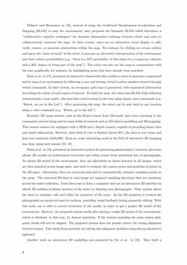
Recently, 3D range sensors, such as the Kinect sensor from Microsoft, have been emerging in the
community and are being used in many fields of research such as 3D objects modelling and 3D mapping.
This sensors sensors are equipped with a RGB and a Depth camera, capable of providing dense color
and depth information. However, their field of view is limited (about 60o), the data is very noisy and
have low resolution (640x480). Even so, some interesting work in the field of interactive 3D mapping
was done using such sensors [10, 18].
Sinha et al. in [10], presented an interactive system for generating photorealistic, textured, piecewise-
planar 3D models of architectural structures and urban scenes from unordered sets of photographs.
To obtain 3D model of the environment, they use algorithms to detect features in all images, which
are then matched across image pairs, and used to estimate the camera poses and positions of points in
the 3D space. Afterwards, lines are extracted and used to automatically estimate vanishing points in
the scene. The extracted 2D lines in each image are assigned vanishing directions that are consistent
across the entire collection. Users then seat in front a computer and use an interactive 3D interface to
sketch 2D outlines of planar sections of the scene by drawing over photographs. Their system allows
the users to visualize, edit and refine the geometry of the scene. As the 3D geometry is created the
photographs are projected onto its surfaces, providing visual feedback during geometric editing. With
this work, one is able to correct structures in the model, in order to get a proper 3D model of the
environment. However, the proposed system works after having a rough 3D model of the environment,
which is obtained, in this case, by feature matching. If the feature matching for some reason fails,
point clouds will not be aligned. The proposed system does not permit correct the wrong alignment
between frames. This thesis focus precisely on solving this alignment problem using also an interactive
approach.
Another work on interactive 3D modelling was presented by Du et al. in [18]. They built a
4
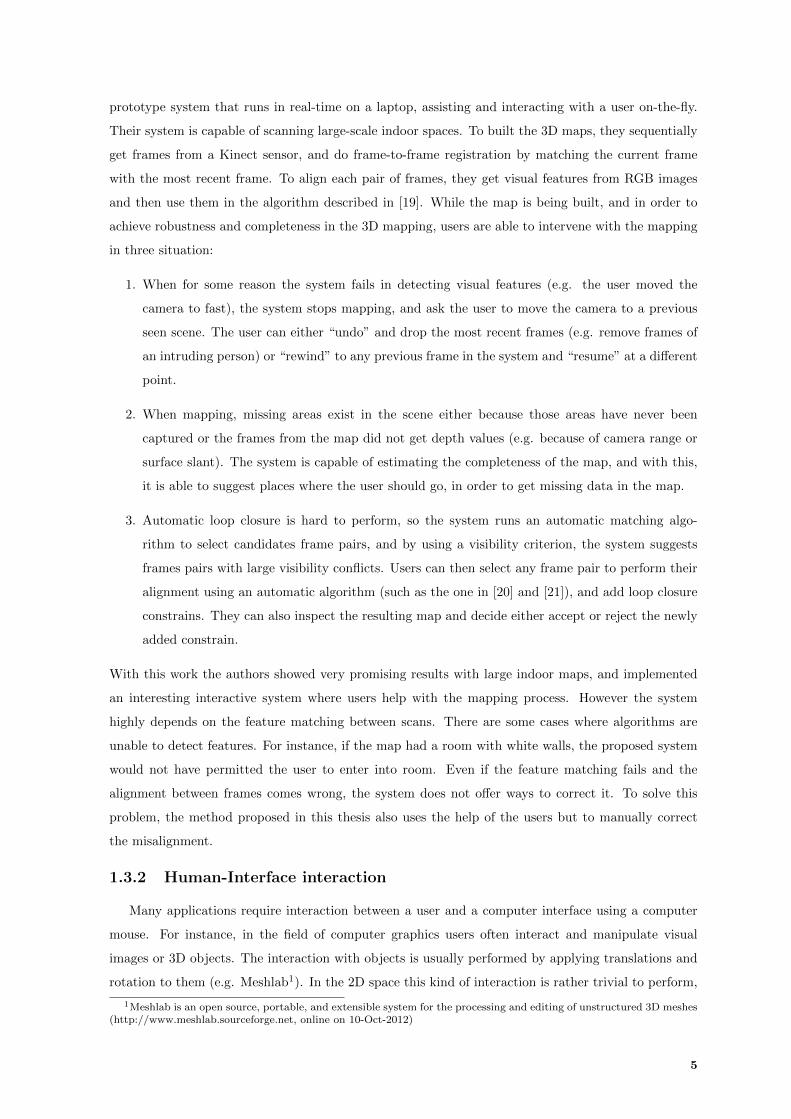
prototype system that runs in real-time on a laptop, assisting and interacting with a user on-the-fly.
Their system is capable of scanning large-scale indoor spaces. To built the 3D maps, they sequentially
get frames from a Kinect sensor, and do frame-to-frame registration by matching the current frame
with the most recent frame. To align each pair of frames, they get visual features from RGB images
and then use them in the algorithm described in [19]. While the map is being built, and in order to
achieve robustness and completeness in the 3D mapping, users are able to intervene with the mapping
in three situation:
1. When for some reason the system fails in detecting visual features (e.g. the user moved the
camera to fast), the system stops mapping, and ask the user to move the camera to a previous
seen scene. The user can either “undo” and drop the most recent frames (e.g. remove frames of
an intruding person) or “rewind” to any previous frame in the system and “resume” at a different
point.
2. When mapping, missing areas exist in the scene either because those areas have never been
captured or the frames from the map did not get depth values (e.g. because of camera range or
surface slant). The system is capable of estimating the completeness of the map, and with this,
it is able to suggest places where the user should go, in order to get missing data in the map.
3. Automatic loop closure is hard to perform, so the system runs an automatic matching algo-
rithm to select candidates frame pairs, and by using a visibility criterion, the system suggests
frames pairs with large visibility conflicts. Users can then select any frame pair to perform their
alignment using an automatic algorithm (such as the one in [20] and [21]), and add loop closure
constrains. They can also inspect the resulting map and decide either accept or reject the newly
added constrain.
With this work the authors showed very promising results with large indoor maps, and implemented
an interesting interactive system where users help with the mapping process. However the system
highly depends on the feature matching between scans. There are some cases where algorithms are
unable to detect features. For instance, if the map had a room with white walls, the proposed system
would not have permitted the user to enter into room. Even if the feature matching fails and the
alignment between frames comes wrong, the system does not offer ways to correct it. To solve this
problem, the method proposed in this thesis also uses the help of the users but to manually correct
the misalignment.
1.3.2 Human-Interface interaction
Many applications require interaction between a user and a computer interface using a computer
mouse. For instance, in the field of computer graphics users often interact and manipulate visual
images or 3D objects. The interaction with objects is usually performed by applying translations and
rotation to them (e.g. Meshlab1). In the 2D space this kind of interaction is rather trivial to perform,
1Meshlab is an open source, portable, and extensible system for the processing and editing of unstructured 3D meshes(http://www.meshlab.sourceforge.net, online on 10-Oct-2012)
5
however it becomes harder when 2D controllers are used to manipulate objects in the 3D space, due
the increase of the Degrees of Freedom (DoF).
Applying rotations to 3D objects using 2D controllers is not an easy task. Chen et al. in [22]
described and evaluated the design of four virtual controllers to rotate objects using a computer mouse.
They conducted a user study, where users were asked to manipulate 3D objects using four types of
controllers: two of them with graphical sliders to control each degree of freedom, one to control the
three DoF by moving the mouse up-down, left-right and in the diagonal, and one that simulates the
mechanics of a physical 3D trackball that can freely rotate about any arbitrary axis in the 3D space
(virtual sphere). The study showed that the users preferred the last controller (virtual sphere) over
the others for being more “natural”.
Later, Bade et al. in [23] did an usability comparison of four mouse-based interaction techniques
based on four principles for 3D rotations techniques. Two of the techniques used in the study were an
improvement to the virtual sphere proposed by Chen et al. in [22] (the Bell’s Virtual Trackball and
the Shoemake’s Virtual Trackball), the third one was the Two-Axis Valuator Trackball also described
in [22] and the last one was a variant of the previous one. The comparison was evaluated with a user
study, which aimed to see which rotation method was most comfortable and predictable for the users.
The study showed that users preferred the “Two-Axis Valuator Trackball”.
Recently Zhao et al. in [24] also did a comparison between the same rotation methods as Bade et
al., but in all techniques the third degree of freedom was controlled by the mouse-wheel. In the user
study they did, they did not find significant performance difference for each method. Although most
users gave positive feedback on using the mouse wheel, it is important to note that the increment of
the wheel must be carefully adjusted overtime because there are times when users want to perform
large rotations and other times when users just want to do slight rotations.
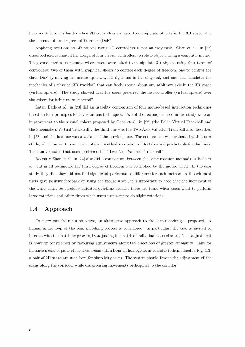
1.4 Approach
To carry out the main objective, an alternative approach to the scan-matching is proposed. A
human-in-the-loop of the scan matching process is considered. In particular, the user is invited to
interact with the matching process, by adjusting the match of individual pairs of scans. This adjustment
is however constrained by favouring adjustments along the directions of greater ambiguity. Take for
instance a case of pairs of identical scans taken from an homogeneous corridor (schematized in Fig. 1.3,
a pair of 2D scans are used here for simplicity sake). The system should favour the adjustment of the
scans along the corridor, while disfavouring movements orthogonal to the corridor.
6

mouse dragFm
Fr DM
scan adjustment
common area
Figure 1.3: Top view of 2 corridors. The scan D is adjusted such that the reaction force Fr, computed fromthe cost function gradient, balances the force Fm imposed by the mouse drag. Scan M and D are correctlyaligned when both common areas are overlapping.
The proposed method is based on a Graphical User Interface (GUI), where the user interacts with
the system using a common computer interface (mouse and keyboard). Consider a pair of range scans
denoted M (for model) and D (for data). Fig. 1.3 illustrates the situation for the corridor example.
When the user drags one of the range scans, say scan D, using the mouse, a corresponding virtual force
Fm is produced (proportional to the drag vector). Opposing it, a reaction force Fr is computed based
in the match between scans M and D. Considering the scan-matching cost function as a potential
function, the symmetric of its gradient with respect to the shift of scan D can be seen as a reaction
force Fr. This reaction force “attracts” scan D towards M , along the direction of less ambiguity. Scan
D is then moved such that both forces become balanced, Fm + Fr = 0. In the corridor example of
Fig. 1.3, the reaction force is dominantly orthogonal to the corridor axis.
The proposed method was first developed and tested in the 2D space and then extended to the 3D
space. A Nomadic Scout robot with a Light Detection And Ranging (LIDAR) onboard is used to take
2D scans while a Microsoft Kinect sensor is used to obtain 3D scans. In both dimensional spaces, scans
are sequentially obtained and the current frame is matched with the most recent frame by computing
a rigid transformation. Both scans and transformations are organized in a data structure kept in the
computer memory, and can be used for posterior analysis at any time.
To build the map of the environment, the Iterative Closest Points (ICP) algorithm (see section 2.2)
is used to obtain the initial rigid transformation between M and D automatically. Then, the proposed
method is used to correct any ambiguity in the alignment. Note that there are other automatic
scan-matching algorithms2 that have better performance than ICP. The ICP is used for the sake of
simplicity.
1.5 Main Contributions
This thesis addresses the problem of scan-matching using an interactive approach. In order to align
pairs of scans or point clouds, users interact with them through a GUI using a simple computer mouse
and keyboard. To help the users in the alignment process, this thesis contributed with a method,
called “Interactive Alignment”, which uses virtual forces to restrain the movement of the range scans.
Scans are aligned by balancing a force produced by a mouse drag (mouse force) with a reaction force
produced by a potential field (reaction force). The proposed method was first developed in the 2D
2see RGBDSLAM in http://www.ros.org/wiki/rgbdslam (retrieved 10-Oct-2012)
7
space and the extended to the 3D space, and does not require an initial alignment between frames to
work. To validate the method, an user study is presented for each dimensional space (2D and 3D).
The following publications resulted directly from this thesis:
1. 10th IEEE International Symposium on Safety Security and Rescue Robotics (SSRR 2012), [25]
2. 17th IEEE International Conference on Emerging Technologies & Factory Automation (ETFA
2012), [26]
3. 1st International Workshop on Perception for Mobile Robots Autonomy (PEMRA 2012), [27]
4. Journal of Automation, Mobile Robotics & Intelligent Systems (JAMRIS), [28] (in press)
1.6 Thesis Outline
This dissertation is organized as follows: Chapter 2 provides background on the shape-based reg-
istration problem and presents the registration method used in this dissertation. Ways of handling
outliers in the Data, and for dealing with convergence to local minima are discussed. Also, the method
represent range scans in memory, as well as how the map is build from them is described. Chapter 3
proposes the method for interactive mapping. First, the method is formalized for the 2D space and
then expanded to the 3D space. Chapter 4 presents the results together with an user study conducted
to evaluate the performance of the proposed method in each dimensional space (2D and 3D). Finally,
Chapter 5 draws some conclusions and discuss possible future work directions. Appendix A and B
covers details concerning the interactive interfaces implemented in this thesis, and appendix C has the
results obtained in both user studies.
8

2Registration Problem
Contents2.1 Problem Statement . . . . . . . . . . . . . . . . . . . . . . . . . . . . . . . . 10
2.2 Iterative Closest Points Algorithm . . . . . . . . . . . . . . . . . . . . . . . 10
2.3 ICP Inicialization . . . . . . . . . . . . . . . . . . . . . . . . . . . . . . . . . 16
2.4 Map Representation . . . . . . . . . . . . . . . . . . . . . . . . . . . . . . . . 19
9
The goals of this chapter are to provide background on the shape-based registration problem,
familiarize the reader with the registration solution method used in this dissertation, and present the
data structure used to keep map in the computer memory.
2.1 Problem Statement
Registration is the problem of determining the relative pose (position and orientation) between two
scans of the same scene (or object). This is done by using features from both scans. Features can
be either geometric or photometric, and 2D or 3D. The main goal of registration is to find a spatial
transformation which brings the features from both scans into alignment as measured by a suitable
cost metric. The transformation may be either rigid or deformable, and may or may not include a
scale term. The work presented in this thesis concentrates on the problem of rigid registration without
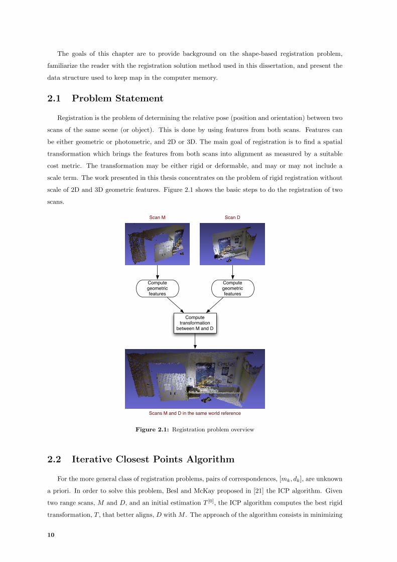
scale of 2D and 3D geometric features. Figure 2.1 shows the basic steps to do the registration of two
scans.
Compute geometricfeatures
Compute geometricfeatures
Scan M Scan D
Compute transformation
between M and D
Scans M and D in the same world reference
Figure 2.1: Registration problem overview
2.2 Iterative Closest Points Algorithm
For the more general class of registration problems, pairs of correspondences, [mk, dk], are unknown
a priori. In order to solve this problem, Besl and McKay proposed in [21] the ICP algorithm. Given
two range scans, M and D, and an initial estimation T [0], the ICP algorithm computes the best rigid
transformation, T , that better aligns, D with M . The approach of the algorithm consists in minimizing
10
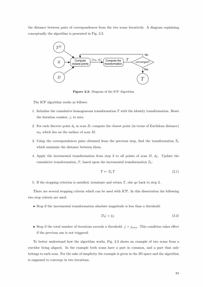
the distance between pairs of correspondences from the two scans iteratively. A diagram explaining
conceptually the algorithm is presented in Fig. 2.2.
Compute closest points
Compute the transformation converged?
Yes
No
M
D
T [0]
T[mk, dk]
T
Figure 2.2: Diagram of the ICP Algorithm
The ICP algorithm works as follows:
1. Initialize the cumulative homogeneous transformation T with the identity transformation. Reset
the iteration counter, j, to zero.
2. For each discrete point dk in scan D, compute the closest point (in terms of Euclidean distance)
mk which lies on the surface of scan M .
3. Using the correspondences pairs obtained from the previous step, find the transformation Tk
which minimize the distance between them.
4. Apply the incremental transformation from step 3 to all points of scan D, dk. Update the
cumulative transformation, T , based upon the incremental transformation Tk:
T ← Tk T (2.1)
5. If the stopping criterion is satisfied, terminate and return T , else go back to step 2.
There are several stopping criteria which can be used with ICP. In this dissertation the following
two stop criteria are used:
• Stop if the incremental transformation absolute magnitude is less than a threshold:
|Tk| < ξT (2.2)
• Stop if the total number of iterations exceeds a threshold: j > jmax. This condition takes effect
if the previous one is not triggered.
To better understand how the algorithm works, Fig. 2.3 shows an example of two scans from a
corridor being aligned. In the example both scans have a part in common, and a part that only
belongs to each scan. For the sake of simplicity the example is given in the 2D space and the algorithm
is supposed to converge in two iterations.
11

1st Iteration 2nd Iteration
Scan MScan D
Compute Closest Points Compute Closest Points
Compute transformation Tand apply it to Data points
Compute transformation Tand apply it to Data points
Scan M and D align!
Figure 2.3: Example of two portions of a corridor (Scan M and D) being align with the ICP algorithm. Inblue is the scan M, in green is the scan D and the red strokes are the distance between closest point from bothscans.
12

2.2.1 Closest Points
In each iteration, the ICP algorithm starts by computing pairs of points composed by matched
points from each scan, which are then used to find the transformation that align both scans. These
pairs of points are created by computing the closest points from one scan (D) to the other (M). The
diagram presented in Fig. 2.4 shows the steps done by the algorithm to get these pairs of points.
Select points from D
Match them with points in M Weight pairs Reject some
pairs
Compute Closest Points
D
M
T [0]
[mk, dk]
Figure 2.4: Diagram showing the steps to compute the closest points to each scan.
Each stage of the algorithm can be implemented using methods that have already been proposed
in the literature. In particular, Rusinkiewicz and Levoy did a comparison between methods for each
stage of the algorithm in [29] with respect to time (number of iterations needed by ICP to converge)
and performance, and proposed a high-speed ICP algorithm variant.
For the Selecting stage of the algorithm, one can use all points available in the scan, like Besl
did when introduced the ICP algorithm in [21] or simply random sampling with a different sample of
points at each iteration, like Masuda did in [30]. The ICP implemented in this thesis, uses all points
when the data obtained from the sensor is below a threshold (number of point below 1000), otherwise
uses random sampling as suggested by Rusinkiewicz and Levoy in [29]. In the end of this stage a set
of points from scans D is obtained: {dk}.The most computationally expensive step in the ICP algorithm is finding the closest points. Al-
though Rusinkiewicz and Levoy suggested using projection-based algorithm to generate point corre-
spondences in the Matching stage, in this thesis K-dimensional trees (Kd-trees) are used to compute
closest points. Kd-trees are special cases of binary space partitioning trees used to organizing points
in a k-dimensional space. Zhang demonstrated in [31] that the average complexity of a closest point
query can be reduced from O(NDNM ) to O(NDlogNM ) using these trees (where NM and ND are the
number of points in scans M and D respectively). By building the tree of scan M and searching in it
for the closest point to {dk}, pairs of correspondences [mk, dk] are obtained.
After obtaining the points correspondences, pairs are weighted in the Weighting stage of the
algorithm, based on the distance between points in each pair. As suggested by Rusinkiewicz and Levoy,
in this thesis, constant weighting is also used to weight pairs. The method is shown in algorithm 2.1
where wk is the weight of pair k and ξmaxCP is the maximum distance allowed between points in one
pair.
Finally, in the last stage of the algorithm, the Rejecting, pairs that have weight equal to zero are
discarded. In end of this stage a new set of pairs [mk, dk] is obtained, and is ready to be used in the
last step of the ICP algorithm. In each iteration of the algorithm, scans M and D get near to each
other. If the same threshold ξmaxCP is used in each iteration, some outliers pairs might not be rejected.
13

Algorithm 2.1 Weighting
if ||mk − Tdk|| < ξmaxCP thenwk ← 0
elsewk ← 1
end if
In order to improve the outliers removal, Zhang proposed in [31] a method to adaptively update ξmaxCP
in each iteration by analysing distances statistics (algorithm 2.2).
Algorithm 2.2 Threshold update for better outliers removal
if µ < ξCP then . The registration is quite goodξmaxCP ← µ+ 3σ
else if µ < 3 ξCP then . The registration is still goodξmaxCP ← µ+ 2σ
else if µ < 6 ξCP then . The registration is not too badξmaxCP ← µ+ σ
else . The registration is really badξmaxCP ← x
end if
The update of threshold ξmaxCP is based on the mean µ and the sample deviation σ of the distances
between points in each pair:
µ =1
N
N∑k=1
(mk − Tdk) , (2.3)
σ =
√√√√ 1
N
N∑k=1
((mk − Tdk)− µ)2, (2.4)
where (mk − Tdk) is the distance between points in pair k and N is the number of pairs. If the
registration is really bad, ξmaxCP is updated with the median of the distances (x). Note that before
the ICP algorithm starts, the threshold ξmaxCP is set to kCP ξCP , where kCP is a proportional constant
and ξCP is a threshold used to check the quality of the registration. The method used to choose the
the value of the proportionality constant and the threshold can be found in [31].
2.2.2 Transformation Computation
The last step of the ICP algorithm consists in assigning an error metric based on the pairs of points,
previously obtained, and minimizing it. The following three error metrics have been studied:
1. Point-to-Point;
2. Point-to-Plane;
3. Plane-to-Plane.
The Point-to-Point error metric consists in computing the best rigid transformation by minimizing
the sum of squared distances between corresponding points:
T = arg minT
N∑k=1
‖mk − T dk‖2, (2.5)
14

where N is the number of pairs, {mk} and {dk} are respectively points from M and D in homogeneous
coordinates and T is the rigid transformation in homogeneous coordinates:
T =
[R t0 1
], (2.6)
with
det (R) = 1 and RTR = I. (2.7)
This error metric has closed form solution for determining the rigid transformation that minimizes the
error. Some solution methods have been proposed: Arun et al. in [32] proposed a solution based on
singular value decomposition, Horn et al. proposed a solution based on quaternions and orthonormal
matrices in [33] and [34] respectively, and Walker et al. proposed a solution based on dual quaternions
in [35]. Eggert et. al. in [36] evaluated the numerical accuracy and stability of each of theses methods,
and concluded that the differences among them were small.
The Point-to-Plane error metric was originally introduced by Chen and Medioni [37] as a more
robust and accurate variant of standard ICP. This error metric consists on minimizing the sum of
squared distances from each source point (mk) to the plane containing the destination point (dk) and
the oriented perpendicular normal. The new cost function differs from (2.5) by taking into account
the surface normals at the source point:
T = arg minT
N∑k=1
‖ηk · (mk − T dk) ‖2, (2.8)
where ηk is the surface normal at mk. The Point-to-Plane error metric does not has any closed-form
solutions available. However the least-squares equations may be solved using a generic non-linear
method (e.g. Levenberg-Marquardt), or by linearising the problem as Kok-Lim Low did in [38] by
assuming that incremental rotations are small: sin (θ) ∼ θ and cos (θ) ∼ 1.
The Plane-to-Plane error metric, also known as generalized ICP, was introduced by Segal et al.
in [39] as an improvement to the Point-to-Plane error metric. They proposed to merge the Point-to-
Point and Point-to-Plane error metrics into a single probabilistic framework, and devised a generalised
framework that naturally converges to both of them by appropriately defining the sample covariance
matrices associated with each point. The way that the generalized ICP cost function is derived is
described in [39] and have the following form:
T = arg minT
N∑k=1
(mk − Tdk)T (CMk + TCDk T
T)−1
(mk − Tdk) , (2.9)
where CMk and CDk are covariance matrices associated with the measured points from scan M and D
respectively.
The Point-to-Point error metric can be obtained by setting CMk = I and CDk = 0:
T = arg minT
N∑k=1
(mk − Tdk)T
(mk − Tdk)
= arg minT
N∑k=1
‖ (mk − Tdk) ‖2, (2.10)
15
which is identical to (2.5). This also shows that Point-to-Point error metric does not takes into account
the structural shape of each scan.
The Point-to-Plane error metric is obtained by setting CMk = P−1k and CDk = 0, where Pk = ηTk ηk
is the projection onto the span of surface normal at mk:
T = arg minT
N∑k=1
(mk − Tdk)TPk (mk − Tdk)
= arg minT
N∑k=1
‖ηk · (mk − Tdk) ‖2. (2.11)
This cost function is identical to (2.8). This also shows that Point-to-Plane error metric only takes
into account the structural shape of scan M .
The Plane-to-plane is obtained when setting CMk 6= 0 and CDk 6= 0. This method improves the ICP
algorithm by exploiting the locally planar structure of both scans. This error metric also does not
has close form solution. However the problem may be solved using a generic non-linear method (e.g.
Levenberg-Marquardt).
2.3 ICP Inicialization
As said before the ICP algorithm receives as input the initial transformation between the two
scans being aligned. This transformation can be either initialized with the identity matrix or with a
precomputed matrix, and it highly influences the effectiveness of the algorithm.
There are many solutions available in the literature to get the initial transformation between two
scans. In this thesis two different methods are used for both 2D and 3D spaces, and using different
sensors.
In 2D space, we only have access to the depth information provided by the laser sensor, thus the
odometry of the robot together with a simple implementation of an Extended Kalman Filter (EKF) are
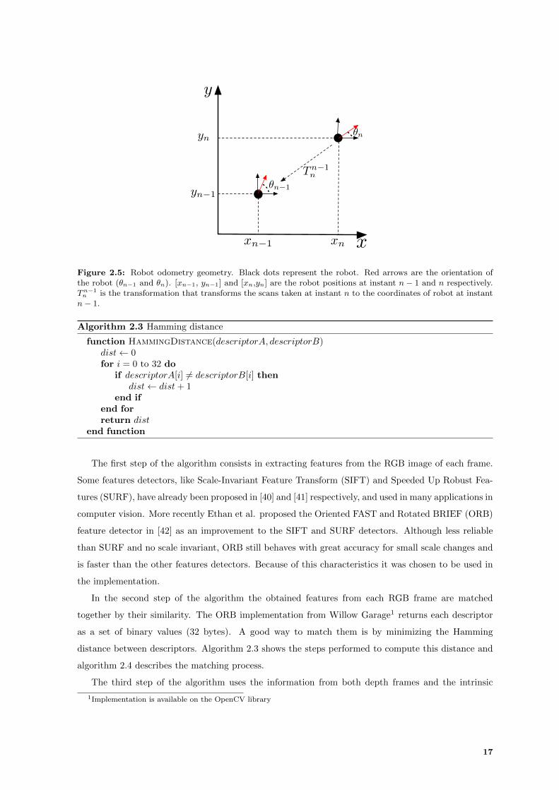
used get the position and orientation of the sensor along time. Figure 2.5 shows the robot odometry
geometry. The transformation which transforms the scans taken at instant n to the coordinates of
robot at instant n− 1, can be obtained by doing:
Tn−1n =
cos (θn − θn− 1) − sin (θn − θn− 1) xn − xn−1sin (θn − θn− 1) cos (θn − θn− 1) yn − yn−1
0 0 1
, (2.12)
where [xn−1,yn−1,θn−1] and [xn,yn,θn] are the positions and orientations of the robot at instant n− 1
and n respectively. This transformation is then used to initialize the ICP algorithm (T [0]).
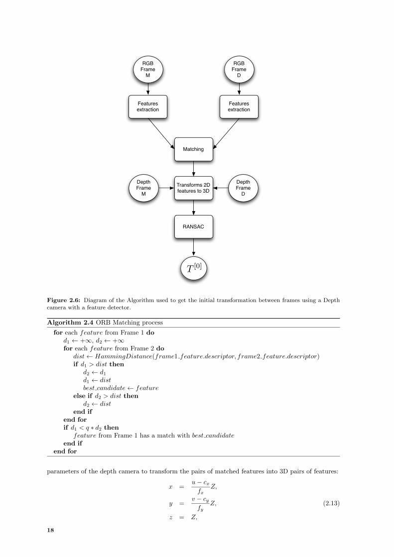
In the 3D space a Microsoft Kinect sensor was used to get 3D scans. When using a robot with a
Kinect onboard, the same method used in the 2D method to obtain the initial transformation can be
applied. On the contrary, when the Kinect is used freely by a user, a similar algorithm based on vision
features to the one proposed by Henry et al. in [19], can be used. In Fig. 2.6 is presented an overview
of the algorithm, which consists in using the information provided by the RGB and depth cameras to
compute features from both frames and use them to compute the best rigid transformation that align
them.
16
✓n�1
✓n
xn�1 xn
yn�1
yn
y
x
Tn�1n
Figure 2.5: Robot odometry geometry. Black dots represent the robot. Red arrows are the orientation ofthe robot (θn−1 and θn). [xn−1, yn−1] and [xn,yn] are the robot positions at instant n− 1 and n respectively.Tn−1n is the transformation that transforms the scans taken at instant n to the coordinates of robot at instantn− 1.
Algorithm 2.3 Hamming distance
function HammingDistance(descriptorA, descriptorB)dist← 0for i = 0 to 32 do
if descriptorA[i] 6= descriptorB[i] thendist← dist+ 1
end ifend forreturn dist
end function
The first step of the algorithm consists in extracting features from the RGB image of each frame.
Some features detectors, like Scale-Invariant Feature Transform (SIFT) and Speeded Up Robust Fea-
tures (SURF), have already been proposed in [40] and [41] respectively, and used in many applications in
computer vision. More recently Ethan et al. proposed the Oriented FAST and Rotated BRIEF (ORB)
feature detector in [42] as an improvement to the SIFT and SURF detectors. Although less reliable
than SURF and no scale invariant, ORB still behaves with great accuracy for small scale changes and
is faster than the other features detectors. Because of this characteristics it was chosen to be used in
the implementation.
In the second step of the algorithm the obtained features from each RGB frame are matched
together by their similarity. The ORB implementation from Willow Garage1 returns each descriptor
as a set of binary values (32 bytes). A good way to match them is by minimizing the Hamming
distance between descriptors. Algorithm 2.3 shows the steps performed to compute this distance and
algorithm 2.4 describes the matching process.
The third step of the algorithm uses the information from both depth frames and the intrinsic
1Implementation is available on the OpenCV library
17
RGBFrame
M
RGBFrame
D
Features extraction
Features extraction
Matching
RANSAC
Transforms 2D features to 3D
DepthFrame
M
DepthFrame
D
T [0]
Figure 2.6: Diagram of the Algorithm used to get the initial transformation between frames using a Depthcamera with a feature detector.
Algorithm 2.4 ORB Matching process
for each feature from Frame 1 dod1 ← +∞, d2 ← +∞for each feature from Frame 2 do
dist← HammingDistance(frame1 feature.descriptor, frame2 feature.descriptor)if d1 > dist then
d2 ← d1d1 ← distbest candidate← feature
else if d2 > dist thend2 ← dist
end ifend forif d1 < q ∗ d2 then
feature from Frame 1 has a match with best candidateend if
end for
parameters of the depth camera to transform the pairs of matched features into 3D pairs of features:
x =u− cxfx
Z,
y =v − cyfy
Z, (2.13)
z = Z,
18
where (u,v) is the coordinates of a feature pixel, (x,y,z) is the coordinates of a 3D feature, Z is the
depth value provided by the depth frame and (cx,cy,fx,fy) are the depth camera intrinsic parameters.
Note that if a feature have Z = 0 or Z = NaN (Not a Number) the corresponding pair is discarded.
Finally, the RANdom SAmple Consensus (RANSAC) method (see [20]) is used in the 3D pairs of
features obtained, to estimate the best rigid transformation that align scan M with scan D. RANSAC
is an iterative method that estimate parameters of a mathematical model from a set of observed data
which contains outliers. In this case the rigid transformation model is used:
mk = T [0] dk, (2.14)
where [mk,dk] is a pair of 3D features and T [0] is homogeneous rigid transformation constituted by a
rotation R and a translation t, which are estimated by RANSAC:
T [0] =
[R t0 1
]. (2.15)
Note that when using a robot, it is possible to use both methods (vision and odometry) to get
initial transformation between two consecutive scans, for instance, when the robot enters in a place
with low level of features and the vision based method fails, the odometry can be used instead.
2.4 Map Representation
Range scans are obtained sequentially from a range sensor and kept in the computer memory. In
this thesis, 2D range scans are obtained with a Nomadic Scout robot with a Hokuyo LIDAR onboard,
while 3D range scans are obtained using the Microsoft kinect sensor.
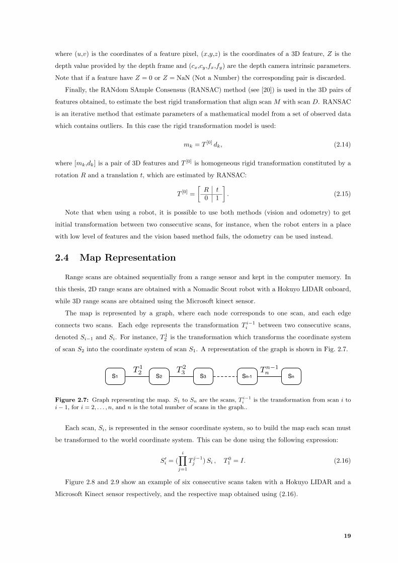
The map is represented by a graph, where each node corresponds to one scan, and each edge
connects two scans. Each edge represents the transformation T i−1i between two consecutive scans,
denoted Si−1 and Si. For instance, T 12 is the transformation which transforms the coordinate system
of scan S2 into the coordinate system of scan S1. A representation of the graph is shown in Fig. 2.7.
S1 S2 Sn-1 SnT 1
2 T 23 S3
Tn−1n
Figure 2.7: Graph representing the map. S1 to Sn are the scans, T i−1i is the transformation from scan i to
i− 1, for i = 2, . . . , n, and n is the total number of scans in the graph..
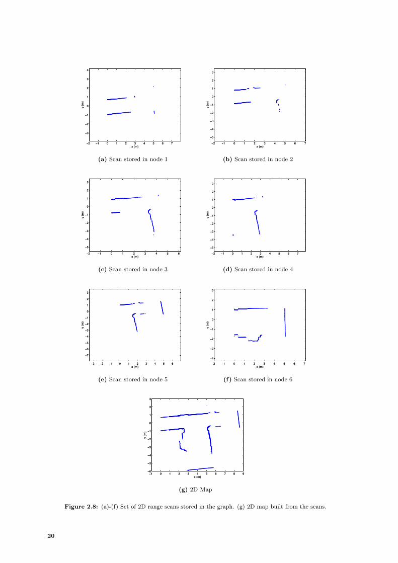
Each scan, Si, is represented in the sensor coordinate system, so to build the map each scan must
be transformed to the world coordinate system. This can be done using the following expression:
S′i = (
i∏j=1
T j−1j )Si , T 01 = I. (2.16)
Figure 2.8 and 2.9 show an example of six consecutive scans taken with a Hokuyo LIDAR and a
Microsoft Kinect sensor respectively, and the respective map obtained using (2.16).
19
−2 −1 0 1 2 3 4 5 6 7
−3
−2
−1
0
1
2
3
4
x (m)
y (
m)
(a) Scan stored in node 1
−2 −1 0 1 2 3 4 5 6 7
−5
−4
−3
−2
−1
0
1
2
3
x (m)
y (
m)
(b) Scan stored in node 2
−2 −1 0 1 2 3 4 5 6
−5
−4
−3
−2
−1
0
1
2
3
x (m)
y (
m)
(c) Scan stored in node 3
−2 −1 0 1 2 3 4 5 6 7
−5
−4
−3
−2
−1
0
1
2
3
x (m)
y (
m)
(d) Scan stored in node 4
−3 −2 −1 0 1 2 3 4 5 6
−7
−6
−5
−4
−3
−2
−1
0
1
2
3
x (m)
y (
m)
(e) Scan stored in node 5
−2 −1 0 1 2 3 4 5 6 7
−4
−3
−2
−1
0
1
2
3
x (m)
y (
m)
(f) Scan stored in node 6
−1 0 1 2 3 4 5 6 7 8 9−6
−5
−4
−3
−2
−1
0
1
2
3
x (m)
y (
m)
(g) 2D Map
Figure 2.8: (a)-(f) Set of 2D range scans stored in the graph. (g) 2D map built from the scans.
20
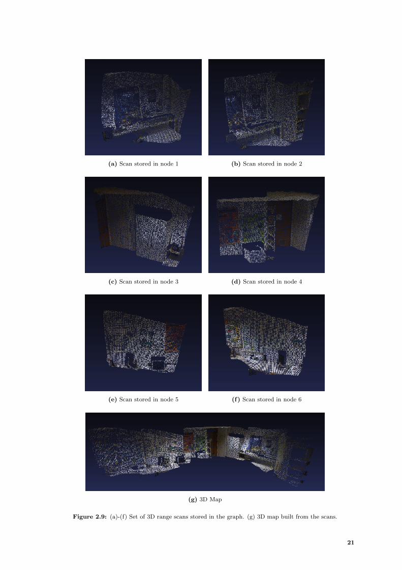
(a) Scan stored in node 1 (b) Scan stored in node 2
(c) Scan stored in node 3 (d) Scan stored in node 4
(e) Scan stored in node 5 (f) Scan stored in node 6
(g) 3D Map
Figure 2.9: (a)-(f) Set of 3D range scans stored in the graph. (g) 3D map built from the scans.
21

22

3Interactive Alignment
Contents3.1 Method Overview . . . . . . . . . . . . . . . . . . . . . . . . . . . . . . . . . 24
3.2 Potential Functions . . . . . . . . . . . . . . . . . . . . . . . . . . . . . . . . 26
3.3 Alignment in 2D . . . . . . . . . . . . . . . . . . . . . . . . . . . . . . . . . . 29
3.4 Extension to 3D . . . . . . . . . . . . . . . . . . . . . . . . . . . . . . . . . . 35
23
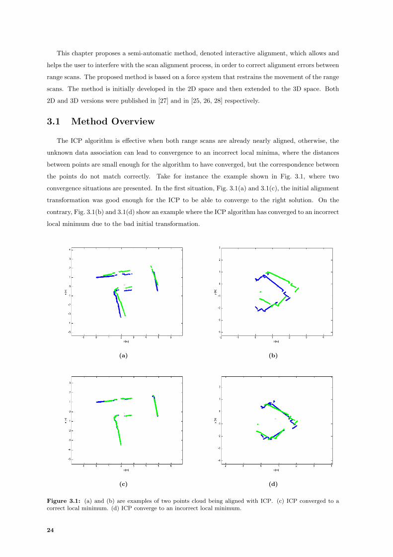
This chapter proposes a semi-automatic method, denoted interactive alignment, which allows and
helps the user to interfere with the scan alignment process, in order to correct alignment errors between
range scans. The proposed method is based on a force system that restrains the movement of the range
scans. The method is initially developed in the 2D space and then extended to the 3D space. Both
2D and 3D versions were published in [27] and in [25, 26, 28] respectively.
3.1 Method Overview
The ICP algorithm is effective when both range scans are already nearly aligned, otherwise, the
unknown data association can lead to convergence to an incorrect local minima, where the distances
between points are small enough for the algorithm to have converged, but the correspondence between
the points do not match correctly. Take for instance the example shown in Fig. 3.1, where two
convergence situations are presented. In the first situation, Fig. 3.1(a) and 3.1(c), the initial alignment
transformation was good enough for the ICP to be able to converge to the right solution. On the
contrary, Fig. 3.1(b) and 3.1(d) show an example where the ICP algorithm has converged to an incorrect
local minimum due to the bad initial transformation.
(a) (b)
(c) (d)
Figure 3.1: (a) and (b) are examples of two points cloud being aligned with ICP. (c) ICP converged to acorrect local minimum. (d) ICP converge to an incorrect local minimum.
24
The ICP algorithm does not guarantee convergence to the correct local minimum, and therefore
the map obtained from the alignment of consecutive pairs of frames may contain enormous errors.
However, by looking closely at Fig. 3.1(d), one can clearly see how the two clouds fit together. Based
on the assumption that users have the perception and capability to judge if the alignment between
two scans needs to be improved, they become active players by interfering with the alignment process,
providing valuable help in the improvement of the scans adjustment.
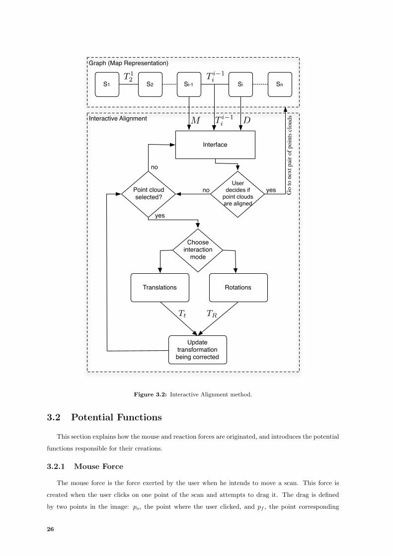
Consider two range scans, Si−1 and Si, each one with N points, stored in two consecutive nodes
in a graph:Si−1 =M = {mk},Si = D = {dk},
mk, dk ∈ R2 ormk, dk ∈ R3 ,
and a rigid transformation in homogeneous coordinates, T i−1i , which align D with M :
T i−1i =
[R t0 1
], (3.1)
where R is a rotation matrix and t is a translation vector. This transformation can be initialized to
a default value (e.g. R = I and t = 0) or computed with an alignment algorithm (e.g. ICP). By
applying this transformation to D, a transformed scan, D′ is obtained. The two scans (M and D′)
are then presented in a viewer (GUI) for alignment analysis. Then, the user decides if M and D are
correctly aligned. If yes, the next pair of scans in the graph is displayed on the interface, if not, in
order to correct their alignment, the user interacts with the viewer using common computer mouse and
keyboard, and apply either translations or rotations to one of the scans (D′). These actions are carried
out separately using a designated key to choose which mode to use. Each time an interactive mode
is used, a new transformation that align D′ with M is obtained. Depending on which mode is used,
we obtain transformation Tt if the mode is translations or transformation TR if the mode is rotations.
These transformations are then applied to the transformation in the graph edge corresponding to the
scan pair being analysed:
T i−1i ← Tt Ti−1i , if translation mode was used, (3.2)
T i−1i ← TR Ti−1i , if rotation mode was used. (3.3)
Figure 3.2 describes how the method works.
The task of manually adjusting pairs of two scans can become time consuming and sometimes
tough, specially when the alignment is being performed in the 3D space, where the interaction with
scans (translations and rotations) using a computer mouse is harder due to the increase of the DoF
from three to six.
In order to help the user in the alignment process, this thesis proposes a force based system that
restrain the movement of the scans. Scans are aligned by balancing a virtual force caused by a mouse
drag, henceforth called mouse force, with a reaction force produced by a potential field.
25
S1 S2 Si
Interface
Chooseinteraction
mode
RotationsTranslations
Update transformationbeing corrected
Sn
User decides if
point clouds are aligned
T 12 T i�1
i
Tt TR
no
yes
Graph (Map Representation)
Interactive Alignment M DT i�1i
Point cloud selected?
no
yes Go
to n
ext p
air o
f poi
nts c
loud
s
Si-1
Figure 3.2: Interactive Alignment method.
3.2 Potential Functions
This section explains how the mouse and reaction forces are originated, and introduces the potential
functions responsible for their creations.
3.2.1 Mouse Force
The mouse force is the force exerted by the user when he intends to move a scan. This force is
created when the user clicks on one point of the scan and attempts to drag it. The drag is defined
by two points in the image: po, the point where the user clicked, and pf , the point corresponding
26
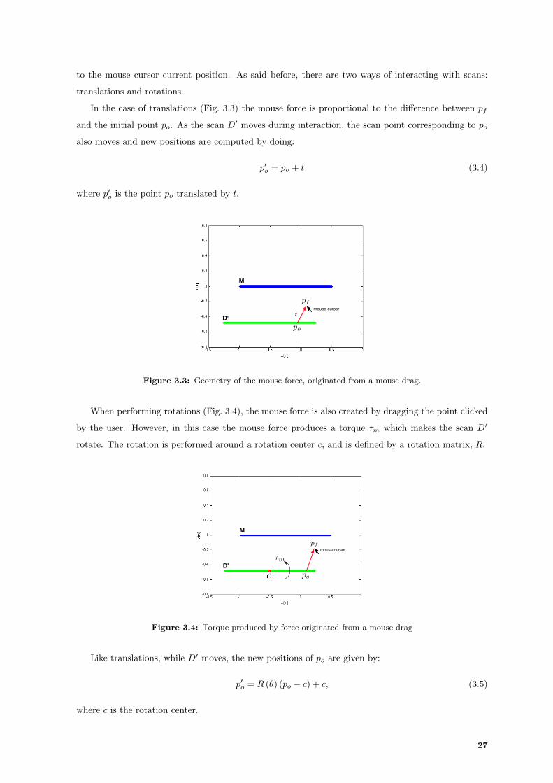
to the mouse cursor current position. As said before, there are two ways of interacting with scans:
translations and rotations.
In the case of translations (Fig. 3.3) the mouse force is proportional to the difference between pf
and the initial point po. As the scan D′ moves during interaction, the scan point corresponding to po
also moves and new positions are computed by doing:
p′o = po + t (3.4)
where p′o is the point po translated by t.
mouse cursorpf
po
M
D' t
Figure 3.3: Geometry of the mouse force, originated from a mouse drag.
When performing rotations (Fig. 3.4), the mouse force is also created by dragging the point clicked
by the user. However, in this case the mouse force produces a torque τm which makes the scan D′
rotate. The rotation is performed around a rotation center c, and is defined by a rotation matrix, R.
po
D'⌧m
mouse cursorpf
M
Figure 3.4: Torque produced by force originated from a mouse drag
Like translations, while D′ moves, the new positions of po are given by:
p′o = R (θ) (po − c) + c, (3.5)
where c is the rotation center.
27

In the general case, the movement of scan D′ is defined by a rigid transformation defined by
a rotation matrix R, a rotation center c and a translation t. Point po is transformed into p′o =
R (po − c) + c+ t. The potential function, Jm, that grows with the distance between points p′o and pf
is defined as follows:
Jm =1
2‖pf − p′o‖2. (3.6)
By taking the gradient of this potential, with respect to either translation t and rotation R, one obtains
the virtual forces and torques induced by the mouse drag:
Fm = −km∇t Jm, (3.7)
τm = −km∇R Jm, (3.8)
where Fm and τm are the force and the torque produced by a mouse drag respectively and km is a
proportionality constant.
3.2.2 Reaction Force
Opposing the mouse force, is the reaction force which is produced by a potential field. This potential
field is defined by threshold ξpot, which creates a region of actuation that makes any scan that enters
in it, be automatically attracted towards M (Fig. 3.5).
⇠pot
�⇠pot
M
⇠pot�⇠pot
(a)
M
D't1
t2
⇠pot
�⇠pot
⇠pot�⇠pot
(b)
Figure 3.5: (a) Potential field of scan M . (b) Reaction force example.
Two scans are attracted to each other by minimizing the distance between corresponding points.
Similarly to ICP algorithm, this minimization consists in computing the best rigid transformation that
aligns D′ with M . For instance, in Fig 3.5(b) a translation t1 is applied to D′ towards M , and as
soon as D′ comes in contact with the potential field, points from D′ are paired with the closest points
of M , producing the reaction force that makes the scan D′ attract towards M . The closest points
are computed in the same fashion as in ICP (using a Kd-tree), and only points that are within the
threshold are considered. These pairs are then used to compute the rigid transformation that better
28
align both scans. The potential function that minimizes the distance between pairs of corresponding
points is given by:
Jr =1
2
N∑k=1
‖mk − [R (dk − c) + c+ t] ‖2, (3.9)
where [mk,dk] are pairs of closest points from M to D′, and N is the number of these pairs. This
function is similar to the potential cost function ICP, with the difference of rotations being performed
about a center of rotation rather than around the origin.
The reaction forces and torques induced by the mouse drag can be obtained bytaking the gradient
of this potential, with respect to either translation t and rotation R:
Fr = −kr∇t Jr, (3.10)
τr = kr∇R Jr, (3.11)
where Fr and τr are the force and the torques induced by the mouse drag respectively and kr is a
proportionality constant.
3.3 Alignment in 2D
This section addresses the two interactive modes which users can use to interact with scans (“Trans-
lations” and “Rotations” blocks from Fig. 3.2) and makes use of the two forces described before to
derive the expressions used to compute the translations and the rotation angles in the 2D space.
3.3.1 Translations
In this mode, the alignment consists in a translation by t. Thus R is the identity, and the potential
functions (3.6) and (3.9) are simplified to:
Jm|R=I =1
2‖pf − (po + t) ‖2, (3.12)
Jr|R=I =1
2
N∑k=1
‖mk − (dk + t) ‖2. (3.13)
The mouse force Fm is computed from the gradient of the potential function (3.12) with respect to
the translation t:
Fm = −km∇t Jm|R=I . (3.14)
Opposing this force, a reaction force Fr is computed from the gradient of the potential func-
tion (3.13) with respect to the translation t:
Fr = −kr∇t Jr|R=I . (3.15)
The forces can be trivially computed by using the vector derivatives rules to compute the gradients
of (3.14) and (3.15):
Fm = km [pf − (po + t)] , (3.16)
Fr = kr
N∑k=1
[mk − (dk + t)] . (3.17)
29

To find a scan adjustment that balances the mouse and the reaction forces, translations are itera-
tively performed, since each time scan D′ moves, the correspondences among points may change. So,
for each iteration, a translation t is computed by solving the equation
Fm + Fr = 0, (3.18)
with respect to t. This equation has the following algebraic closed form solution:
t =km(pf − po) + kr
∑Nk=1(mk − dk)
km +Nkr. (3.19)
Algorithm 3.1 Compute Translation
function Translation(po, pf ,M,D′)Dnew ← D′
repeatP ← ComputeClosestPoints(M,Dnew)t← ComputeTranslation(po, pf , P )Dnew ← UpdateScan(D′, t)
until ErrorChange(t) < ξtreturn t
end function
The scan adjustment results from the algorithm 3.1. The algorithm receives the mouse initial and
current position and the two scans being adjusted (M and D′) as input. The algorithm starts by
computing a subset, P , of pairs of closest points from the two scans (P ⊂ {[m1, d1]...[mk, dk]}) The
subset P is then used together with the mouse positions in (3.19) to compute the translation. Finally
scan D′ is updated with the new estimate of the translation and the convergence is checked. The
algorithm iterates until the correspondences between points are the same, or in other words until the
norm of the difference between the new and the previous translation estimation falls below a threshold:
‖ti − ti−1‖ < ξt, (3.20)
where ti−1 and ti are the estimation of the translation at iteration i− 1 and i respectively and ξt is a
threshold.
The obtained t = [tx ty]T corresponds to the homogeneous transformation:
Tt =
[I2×2 t
0 1
], (3.21)
where I2×2 is a 2× 2 identity matrix.
Figure 3.6 shows an example of two scans being align by applying translations, with and without
forces. On the left three sub-figure, scan D′ (green) moves freely (mouse current position is the same
as the initial point clicked), due to the absence of the potential field. On the contrary, on the other
three sub-figures the balance of the forces (Fm and Fr) restrain the movement of the scan by favouring
the adjustment along the corridor, while disfavouring movements orthogonal to the corridor.
30
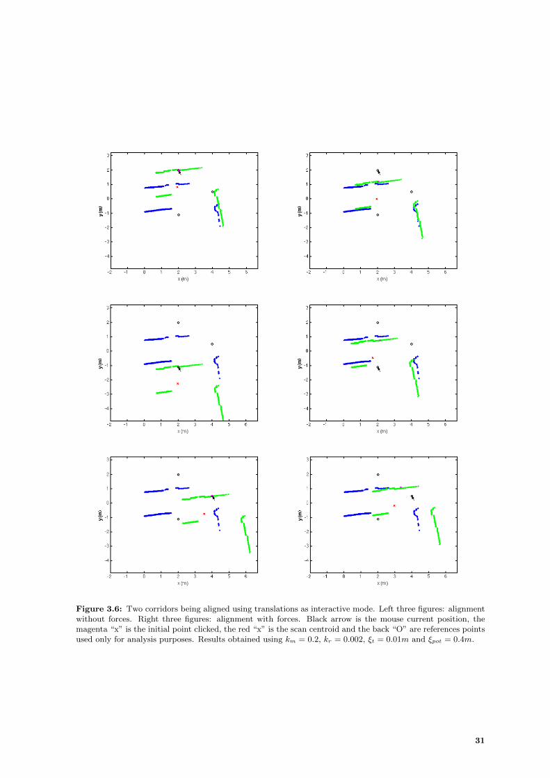
Figure 3.6: Two corridors being aligned using translations as interactive mode. Left three figures: alignmentwithout forces. Right three figures: alignment with forces. Black arrow is the mouse current position, themagenta “x” is the initial point clicked, the red “x” is the scan centroid and the back “O” are references pointsused only for analysis purposes. Results obtained using km = 0.2, kr = 0.002, ξt = 0.01m and ξpot = 0.4m.
31

3.3.2 Rotations
In the Euclidean space, the rotation of one point in the xy-Cartesian plane through an angle θ
about the origin, can be performed using the usual rotation matrix:
R (θ) =
[cos (θ) − sin (θ)sin (θ) cos (θ)
]. (3.22)
Rotation mode comprises a rotation of scan D′, with respect to the center of mass c, by an angle θ
(Fig. 3.4). The center of mass of a scan is set to its centroid. When the user clicks on the scan D′ and
attempts to drag it, a force Fm is created using (3.6), for t = 0. The cost functions (3.6) and (3.9) are
simplified to:
Jm|t=0 =1
2‖pf − [R (θ) (po − c) + c]‖2
=1
2‖p′f −R (θ) ri)‖2, (3.23)
Jr|t=0 =1
2
N∑k=1
‖mk − [R (θ) (dk − c) + c]‖2
=1
2
N∑k=1
‖m′k −R (θ) d′k‖2, (3.24)
where ri = (po − c), p′f = (pf − c), m′k = (mk − c) and d′k = (dk − c).However, unlike translations, the balance is formulated here in terms of virtual torques. The mouse
torque τm is the gradient of the cost function (3.23) with respect to θ:
τm = −km∇θ Jm|t=0 . (3.25)
The opposing torque τr is the gradient of the cost function (3.24) with respect to θ:
τr = −kr∇θ Jr|t=0 . (3.26)
Both gradients can be computed using the chain rule:
∇θ Jm|t=0 = tr
[(∂Jm∂R (θ)
)T∂R (θ)
∂θ
], (3.27)
∇θ Jr|t=0 = tr
[(∂Jr∂R (θ)
)T∂R (θ)
∂θ
], (3.28)
and the partial derivatives can be trivially obtained using the matrix and vector derivative rules:
∂Jm∂R (θ)
= −p′frTi , (3.29)
∂Jr∂R (θ)
= −N∑k=1
m′k(d′k)T , (3.30)
∂R (θ)
∂θ=
[− sin (θ) − cos (θ)cos (θ) − sin (θ)
]= AR (θ) , (3.31)
where A =
[0 −11 0
].
32

Both torques are obtained by computing the trace of (3.27) and (3.28) and using the partial
derivatives from (3.29), (3.30) and (3.31) :
τm = km rTi R
TAT p′f , (3.32)
τr = kr
N∑k=1
(d′k)TRT AT m′k. (3.33)
As in the case of translations, the scan D′ is iteratively rotated until convergence of the correspondences
is reached. In each iteration, the balance of torques
τm + τr = 0 (3.34)
has a closed form solution. Using (3.32) and (3.33) in (3.34) we can obtain
tan(θ) =kmr
Ti A
T p′f + kr∑Nk=1(d′k)TAT m′k
kmrTi p′f + kr
∑Nk=1(d′k)Tm′k
. (3.35)
However, this only allows us to compute θ up to a π congruence. To resolve this ambiguity, which is
caused by the existence of two solutions π radians appart, one has to determine which one corresponds
to a stable solution. This can be easily determined from the sign of the derivative of the total torque
τ = τm + τr:
∂τ
∂θ= −kmrTi RT (θ)p′f − kr
N∑k=1
(d′k)TRT (θ)m′k. (3.36)
A solution is stable if and only if the sign of this derivative is negative. A positive derivative implies
that a small perturbation in θ will swing the scan π radians towards the other solution. Note that (3.36)
has opposite signs for angles θ and θ + π, and therefore there is always a single negative solution.
Algorithm 3.2 Compute Rotation Angle
function Rotations(po, pf ,M,D′)c← ComputeScanCentroid(D′)Dnew ← D′
ri ← po − cp′f ← pf − crepeat
P ← ComputeClosestPoints(M,Dnew)for each pair of closest points in P do
m′k ← mk − cd′k ← dk − cP ′ ← (m′k, d
′k)
end forθ ← ComputeRotationAngle(ri, p
′f , P
′)if sign(ComputeTorqueDerivative(θ, ri, p
′f , P
′)) > 0 thenθ ← θ + π
end ifDnew ← UpdateScan(D′, θ)
until ErrorChange(θ) < ξθreturn θ
end function
Algorithm 3.2 shows the steps needed to adjust the scans when performing rotations. The algorithm
starts by computing the scan centroid and used it to center the mouse positions in the origin. In each
33

iteration, new correspondences are obtained and used to compute the rotation angle. The stable
solution is then chosen using (3.36). Finally scan D′ is updated with the new estimate of the rotation
angle and the convergence is checked. The algorithm iterates until the module of the difference between
the new and the previous rotation angle falls below a threshold:
|θi − θi−1| < ξθ, (3.37)
where θi−1 and θi are the estimation of the rotation angle at iteration i − 1 and i respectivelyand ξθ
is a threshold.
A rotation transformation is then created using the value θ,
TR =
cos(θ) − sin(θ) bxsin(θ) cos(θ) by
0 0 1
, (3.38)
b =
[bxby
]= [I −R(θ)] c. (3.39)
Note that translation b accounts for the fact that the rotation is performed with respect to center c,
rather than to the origin.
Figure 3.7 shows an example of two scans being align by applying rotations, without using forces
and using forces. As it can be seen, the balance of the two torques is able to restrain the movement of
the scans.
Figure 3.7: Two corridors being aligned using rotations. Left two figures: alignment without forces. Righttwo figures: alignment with forces. Black arrow is the mouse current position, the magenta “x” is the initialpoint clicked, the red “x” is the point cloud center of mass and the back “O” are references points used onlyfor analysis purposes. Results obtained using km = 0.1, kr = 0.004, ξθ = 0.01m and ξpot = 0.4m
34

3.4 Extension to 3D
This section extends the proposed method to the 3D space. The algorithm and the potential
functions presented in section 3.1 and 3.2 remain the same. The only thing that changes is the way
block “Translations” and “Rotations” from Fig. 3.2 are implemented. Contrary to what happens in the
2D space, in the 3D space the interaction with point clouds using a computer mouse becomes harder
due the increase of the DoF from three to six. Using a computer mouse, one can only control two DoF,
so the interaction between users and point clouds is restricted to a plane parallel to the image plane.
Translation and rotations are performed using mouse forces defined on this plane.
Performing rotations in 3D with a computer mouse is not a trivial task, so the user is allowed to
choose among tree types of rotations, based on previous studies concerning human-computer interaction
with 3D objects:
1. Rotation without restrictions: in this mode the three DoF are taken into account when computing
the rotations matrix (see section 3.4.2);
2. Rotation restrict to a plane (see [22]): in this mode rotations are performed around an axis
orthogonal to the plane parallel to the image plane (see section 3.4.3.A);
3. Rotation using a virtual sphere (see [23]): in this mode the point clicked is projected onto the
image plane and used alongside the mouse current position in the image plane to compute the
rotation axis and the angle each time the mouse moves (see section 3.4.3.B).
3.4.1 Translations
In 3D, we only have access to the coordinates of the pixel of the mouse current position in the
image plane, therefore the mouse force is defined on a 3D plane parallel to the image plane. The drag
is defined by two 3D points, po and pf , corresponding to the initial and final drag points. When the
user clicks on point could D′, the initial point po is set to the point on D′ which projection on the
image plane is closest to the mouse point clicked by the user. As the user drags the mouse, pf is defined
by the projection of the new mouse point onto the plane parallel to the image plane that crosses po
(Fig. 3.8). As point cloud D′ moves during interaction, the point corresponding to po also moves.
The mouse force, produced by a mouse drag, is obtained using po and pf in the potential func-
tion (3.6), and by computing its gradient with respect to the translation t, when there is no rotation,
R = I3×3. The result obtained is the same as (3.16).
The reaction force is also obtained by computing the gradient of the potential function (3.9) with
respect to the translation t when the rotation R = I3×3. The closest points ({mk} and {dk}) are
computed in the same way as in ICP (Kd-trees) and only the pairs sufficiently close are considered.
The result obtained is the same as (3.17).
By balancing the two forces, Fm + Fr = 0, we obtain the same close form solution as the one
obtained for translations (3.19) in the 2D space.
The scan adjustment follows the same algorithm as the one described in section 3.3.1. The only
difference is the way po and pf are obtained.
35
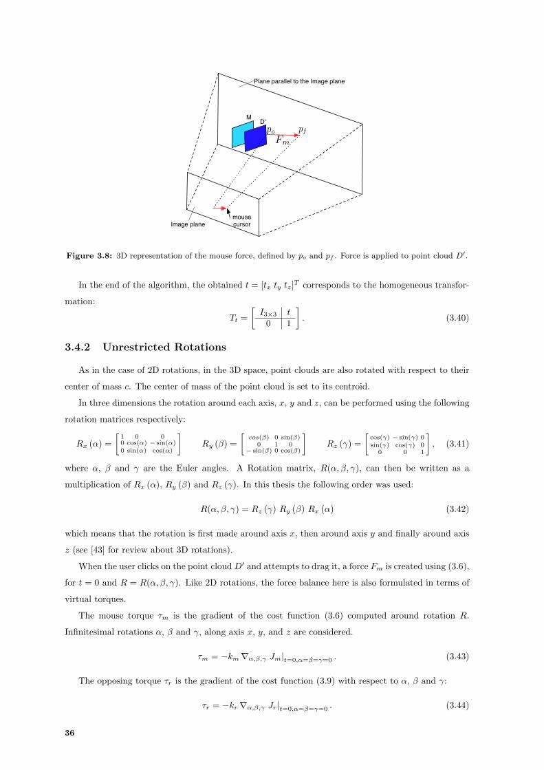
MD'
mousecursorImage plane
Plane parallel to the Image plane
Figure 3.8: 3D representation of the mouse force, defined by po and pf . Force is applied to point cloud D′.
In the end of the algorithm, the obtained t = [tx ty tz]T corresponds to the homogeneous transfor-
mation:
Tt =
[I3×3 t
0 1
]. (3.40)
3.4.2 Unrestricted Rotations
As in the case of 2D rotations, in the 3D space, point clouds are also rotated with respect to their
center of mass c. The center of mass of the point cloud is set to its centroid.
In three dimensions the rotation around each axis, x, y and z, can be performed using the following
rotation matrices respectively:
Rx (α) =
[1 0 00 cos(α) − sin(α)0 sin(α) cos(α)
]Ry (β) =
[cos(β) 0 sin(β)
0 1 0− sin(β) 0 cos(β)
]Rz (γ) =
[cos(γ) − sin(γ) 0sin(γ) cos(γ) 0
0 0 1
], (3.41)
where α, β and γ are the Euler angles. A Rotation matrix, R(α, β, γ), can then be written as a
multiplication of Rx (α), Ry (β) and Rz (γ). In this thesis the following order was used:
R(α, β, γ) = Rz (γ) Ry (β) Rx (α) (3.42)
which means that the rotation is first made around axis x, then around axis y and finally around axis
z (see [43] for review about 3D rotations).
When the user clicks on the point cloud D′ and attempts to drag it, a force Fm is created using (3.6),
for t = 0 and R = R(α, β, γ). Like 2D rotations, the force balance here is also formulated in terms of
virtual torques.
The mouse torque τm is the gradient of the cost function (3.6) computed around rotation R.
Infinitesimal rotations α, β and γ, along axis x, y, and z are considered.
τm = −km∇α,β,γ Jm|t=0,α=β=γ=0 . (3.43)
The opposing torque τr is the gradient of the cost function (3.9) with respect to α, β and γ:
τr = −kr∇α,β,γ Jr|t=0,α=β=γ=0 . (3.44)
36
Note that Euler angles suffer from singularities, however, the rotation is parametrized using a rota-
tion matrix, while the Euler angles are only used for computing derivatives(small angle approximation).
Thus, derivatives in (3.43) and (3.44) are done around the point α = 0, β = 0 and γ = 0.
Both gradients can be computed using the chain rule:
∇α,β,γ Jm|t=0,α=β=γ=0 =
[tr
[(∂Jm
∂R (α, β, γ)
)T∂R (α, β, γ)
∂x
]], (3.45)
∇α,β,γ Jr|t=0,α=β=γ=0 =
[tr
[(∂Jr
∂R (α, β, γ)
)T∂R (α, β, γ)
∂x
]], (3.46)
where x = α, β and γ.
The partial derivative ∂R(α,β,γ)∂x can be computed using the derivative definition:
∂R (α, β, γ)
∂x= limx→0
R (x0 + x)−R (x0)
x= limx→0
(R (x)− I)R (x0)
x= AxR (x0) , (3.47)
where x0 = (α, β, γ),
Aα =
0 0 00 0 −10 1 0
, Aβ =
0 0 10 0 0−1 0 0
and Aγ =
0 −1 01 0 00 0 0
.The partial derivative ∂Jm
∂R(α,β,γ) and ∂Jr∂R(α,β,γ) can be trivially obtained by computing the derivative
of expression (3.6) and (3.9) with respect to R (α, β, γ), which has the same result as (3.29) and (3.30):
∂Jm∂R (α, β, γ)
= −p′frTi , (3.48)
∂Jr∂R (α, β, γ)
= −N∑k=1
m′k(d′k)T . (3.49)
Using the results (3.48), (3.49) and (3.47) in (3.45) and (3.46), it is possible to write the expression of
the torques:
τm = −km[tr[ri(p′f)TAxR
]], (3.50)
τr = −kr[tr
[N∑k=1
d′k (m′k)TAxR
]], (3.51)
where x = α, β and γ. Note that the rotation, R, is parametrized using a rotation matrix so:
R =
r11 r12 r13r21 r22 r23r31 r32 r33
(3.52)
where
RTR = I and det (R) = 1 (3.53)
Similarly to 2D rotations, the objective here is also to find the rotation, R, that balances the torques :
τm + τr = 0. (3.54)
Using the result from (3.50) and (3.51) in (3.54) and using the trace properties, three equation are
obtained:
tr
[(kmri
(p′f)T
+ kr
N∑k=1
d′k (m′k)T
)AxR
]= 0, (3.55)
37

where x = α, β and γ. The nine unknown variables referred in (3.52) can be obtained by solving
the non-linear system composed by the three equations in (3.55) and the six equations from the
constrain (3.53):
b13r21 + b23r22 + b33r23 − b12r31 − b22r32 − b32r33 = 0,
−b13r11 − b23r12 − b33r13 + b11r31 − b21r32 + b31r33 = 0,
b12r11 + b22r12 + b32r13 − b11r21 − b21r22 − b31r23 = 0,
r211 + r221 + r231 = 1,
r212 + r222 + r232 = 1, (3.56)
r213 + r223 + r233 = 1,
r11r12 + r21r22 + r31r32 = 0,
r11r13 + r21r23 + r31r33 = 0,
r12r13 + r22r23 + r32r33 = 0,
where
B =
b11 b12 b13b21 b22 b23b31 b32 b33
= kmri(p′f)T
+ kr
N∑k=1
d′k (m′k)T.
The point cloud D′ is iteratively rotated until convergence of the correspondences is reached. In
each iteration, balancing the torques consists in solving the above system. Due to the non-linearity of
the system, a suitable solver1 is used to resolve (3.56).
Algorithm 3.3 summarizes the steps needed to perform the point clouds adjustment. The algorithm
framework is similar to the one in 2D rotations. The way points po and pf are obtained and the
condition to check the convergence (ErrorChange) are the only changes.
Algorithm 3.3 Compute Rotation Matrix
function UnrestrictedRotation(po, pf ,M,D′)c← ComputeScanCentroid(D′)Dnew ← D′
ri ← po − cp′f ← pf − crepeat
P ← ComputeClosestPoints(M,Dnew)for each pair of closest points in P do
m′k ← mk − cd′k ← dk − cP ′ ← (m′k, d
′k)
end forR← ComputeRotationMatrix(ri, p
′f , P
′)Dnew ← UpdateScan(D′, R)
until ErrorChange(R) < ξRreturn R
end function
The balanced of the forces is achieved when the difference between the rotation angle computed
in iteration i − 1 and i falls below a threshold ξR. The angular difference can be obtained from the
1A variation of the Levenberg Marquardt algorithm was used, as implemented in Eigen library(http://eigen.tuxfamily.org, online on 10-Oct-2012).
38
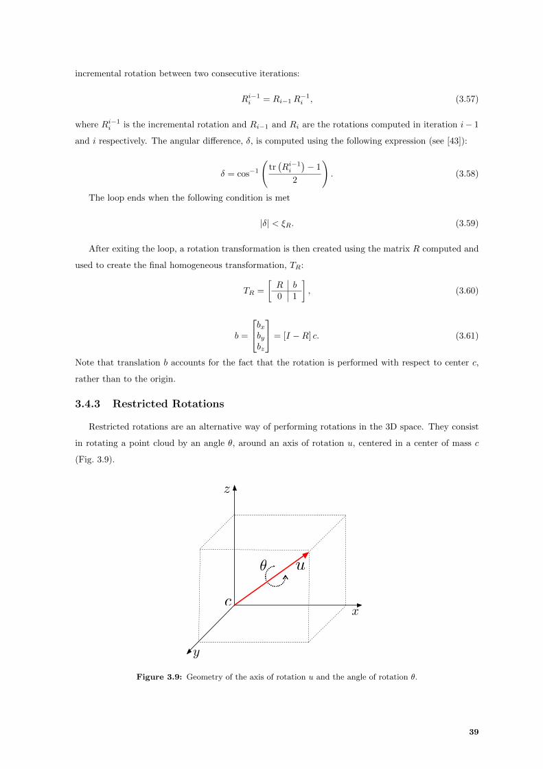
incremental rotation between two consecutive iterations:
Ri−1i = Ri−1R−1i , (3.57)
where Ri−1i is the incremental rotation and Ri−1 and Ri are the rotations computed in iteration i− 1
and i respectively. The angular difference, δ, is computed using the following expression (see [43]):
δ = cos−1(
tr(Ri−1i
)− 1
2
). (3.58)
The loop ends when the following condition is met
|δ| < ξR. (3.59)
After exiting the loop, a rotation transformation is then created using the matrix R computed and
used to create the final homogeneous transformation, TR:
TR =
[R b0 1
], (3.60)
b =
bxbybz
= [I −R] c. (3.61)
Note that translation b accounts for the fact that the rotation is performed with respect to center c,
rather than to the origin.
3.4.3 Restricted Rotations
Restricted rotations are an alternative way of performing rotations in the 3D space. They consist
in rotating a point cloud by an angle θ, around an axis of rotation u, centered in a center of mass c
(Fig. 3.9).
✓ u
z
x
y
c
Figure 3.9: Geometry of the axis of rotation u and the angle of rotation θ.
39
The DoF are reduced from three to one. The rotation matrix is given by the Rodrigues’ rotation
formula, which says that given an unit vector u = [ux, uy, uz], where u2x + u2y + u2z = 1, the matrix
which performs a rotation by an angle θ about an axis in the direction of u is:
R (θ) = I cos (θ) + sin (θ) U1 + (1− cos (θ))U2, (3.62)
where
U1 =
0 −uz uyuz 0 −ux−uy ux 0
and U2 =
u2x uxuy uxuz
uxuy u2y uyuz
uxuz uyuz u2z
.There are several axis of rotation that can be used to rotate point clouds around them. Two
particular rotations, described in section 3.4.3.A and 3.4.3.B, can be implemented using different
methods to compute this axis. Once computed, vector u needs to be normalized to meet the constrain
u2x + u2y + u2z = 1:
u =u
‖u‖ . (3.63)
When the user clicks on the point cloud D′ and attempts to drag it, a force Fm is created using (3.6),
for t = 0 and R = R(θ). The expressions of the torques are very similar to the ones derived in 2D
rotations. The mouse torque τm is the gradient of the potential function (3.6) with respect to θ:
τm = −km∇θ Jm|t=0 , (3.64)
and the opposing torque τr is the gradient of the potential function (3.9) with respect to θ:
τr = −kr∇θ Jr|t=0 . (3.65)
Both gradients can be computed using the chain rule:
∇θ Jm|t=0 = tr
[(∂Jm∂R (θ)
)T∂R (θ)
∂θ
], (3.66)
∇θ Jr|t=0 = tr
[(∂Jr∂R (θ)
)T∂R (θ)
∂θ
]. (3.67)
The partial derivative ∂R(θ)∂θ can be computed by making the derivative of (3.62) with respect to θ:
∂R (θ)
∂θ= U1 cos (θ)− (I − U2) sin (θ) . (3.68)
The partial derivatives ∂Jm∂R(θ) and ∂Jr
∂R(θ) have the same result as (3.29) and (3.30) respectively, differing
only on po, ri,mk, dk ∈ R3, m′k = mk − c and d′k = dk − c.The value of the torques can be obtained using (3.29), (3.30) and (3.68) in (3.66) and (3.67):
τm = −km[rTi U
T1 p′f cos (θ)− rTi (I − U2)
Tp′f sin (θ)
], (3.69)
τr = −krN∑k=1
[(d′k)TUT1m
′k cos (θ)− (d′k)T (I − U2)
Tm′k sin (θ)
], (3.70)
where N is the number of pair of closest points.
40
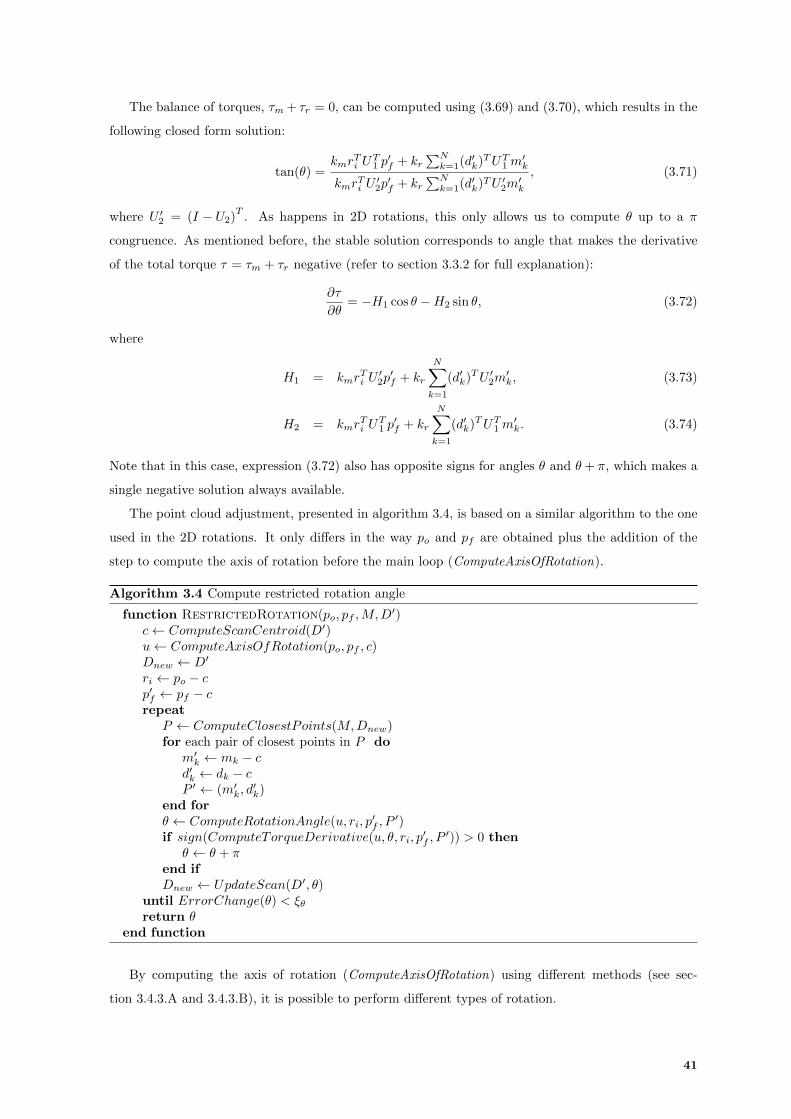
The balance of torques, τm + τr = 0, can be computed using (3.69) and (3.70), which results in the
following closed form solution:
tan(θ) =kmr
Ti U
T1 p′f + kr
∑Nk=1(d′k)TUT1m
′k
kmrTi U′2p′f + kr
∑Nk=1(d′k)TU ′2m
′k
, (3.71)
where U ′2 = (I − U2)T
. As happens in 2D rotations, this only allows us to compute θ up to a π
congruence. As mentioned before, the stable solution corresponds to angle that makes the derivative
of the total torque τ = τm + τr negative (refer to section 3.3.2 for full explanation):
∂τ
∂θ= −H1 cos θ −H2 sin θ, (3.72)
where
H1 = kmrTi U′2p′f + kr
N∑k=1
(d′k)TU ′2m′k, (3.73)
H2 = kmrTi U
T1 p′f + kr
N∑k=1
(d′k)TUT1m′k. (3.74)
Note that in this case, expression (3.72) also has opposite signs for angles θ and θ+ π, which makes a
single negative solution always available.
The point cloud adjustment, presented in algorithm 3.4, is based on a similar algorithm to the one
used in the 2D rotations. It only differs in the way po and pf are obtained plus the addition of the
step to compute the axis of rotation before the main loop (ComputeAxisOfRotation).
Algorithm 3.4 Compute restricted rotation angle
function RestrictedRotation(po, pf ,M,D′)c← ComputeScanCentroid(D′)u← ComputeAxisOfRotation(po, pf , c)Dnew ← D′
ri ← po − cp′f ← pf − crepeat
P ← ComputeClosestPoints(M,Dnew)for each pair of closest points in P do
m′k ← mk − cd′k ← dk − cP ′ ← (m′k, d
′k)
end forθ ← ComputeRotationAngle(u, ri, p
′f , P
′)if sign(ComputeTorqueDerivative(u, θ, ri, p
′f , P
′)) > 0 thenθ ← θ + π
end ifDnew ← UpdateScan(D′, θ)
until ErrorChange(θ) < ξθreturn θ
end function
By computing the axis of rotation (ComputeAxisOfRotation) using different methods (see sec-
tion 3.4.3.A and 3.4.3.B), it is possible to perform different types of rotation.
41

The homogeneous transformation, TR, is then created using the value θ just computed in the
Rodrigues formula (3.62):
TR =
[R (θ) b
0 1
], (3.75)
b =
bxbybz
= [I −R (θ)] c. (3.76)
Note that translation b accounts for the fact that the rotation is performed with respect to center c,
rather than the origin.
3.4.3.A Rotation restricted to a plane
Rotation restricted to a plane is a particular case of restricted rotations. They are performed
about an axis perpendicular to the plane parallel to the image plane, and centered in the center of
mass projected on this plane. Figure 3.10 shows the 3D representation of the axis and the vectors used
to compute it.
Mouse cursor
Plane parallel to the image plane
Point cloud
x(m)
y(m)
z(m)
p
(a) (b)
Figure 3.10: (a) 3D representation of the axis of rotation, u, orthogonal to a plane parallel to the imageplane. po is the point cloud point clicked by the user, c′ is the point cloud centroid c projected onto the planeparallel to the image plane and v1 ⊥ v2 ⊥ u. (b) 3D representation of the axis of rotation from another pointof view.
The axis orthogonal to the plane, u, can be obtained by computing the cross product of two vectors
belonging to the plane:
u = v1 × v2, (3.77)
with v1 = po − c′ and v2 = p− c′, where po is the the point clicked by the user, p is a point belonging
to the plane, c′ is the centroid project onto the plane and v1 ⊥ v2.
Expressions (3.71) and (3.72) are modified in order to use the centroid projected onto the plane c′
instead of c, therefore m′k = mk − c′ and d′k = dk − c′.Algorithm 3.5 shows how the axis of rotation can be computed (ComputeAxisOfRotation) to be
used in scan adjustment algorithm 3.4.
42
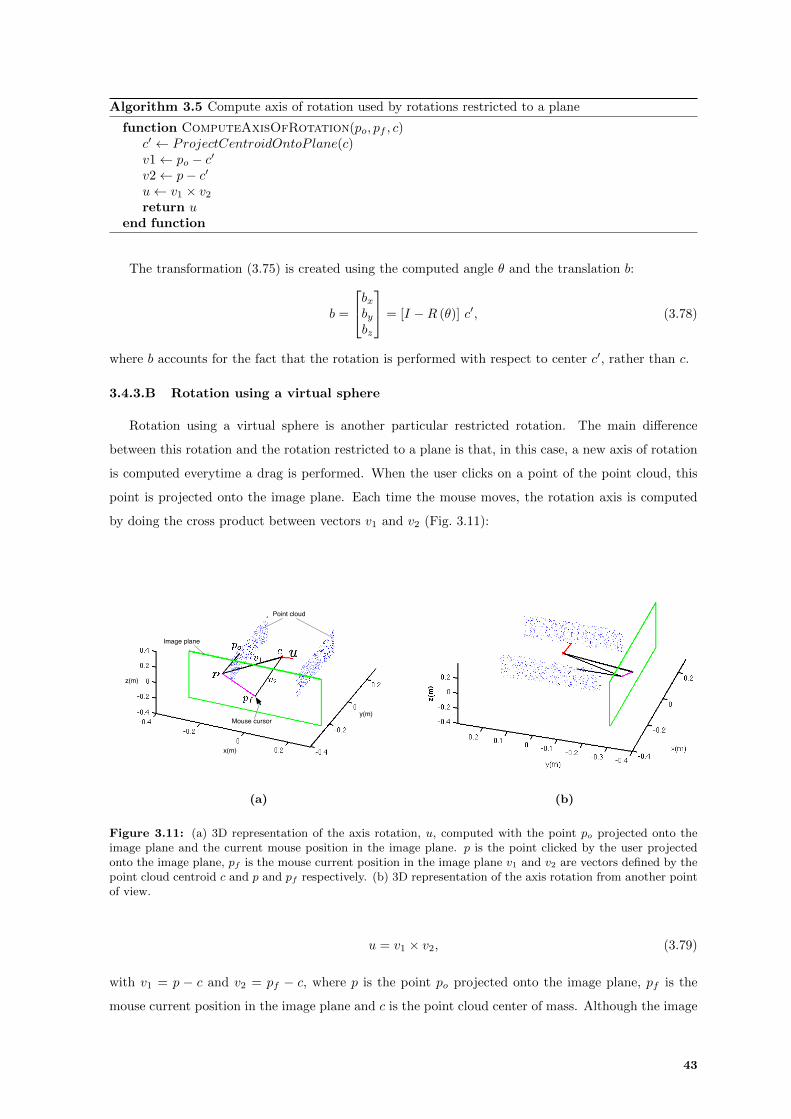
Algorithm 3.5 Compute axis of rotation used by rotations restricted to a plane
function ComputeAxisOfRotation(po, pf , c)c′ ← ProjectCentroidOntoP lane(c)v1← po − c′v2← p− c′u← v1 × v2return u
end function
The transformation (3.75) is created using the computed angle θ and the translation b:
b =
bxbybz
= [I −R (θ)] c′, (3.78)
where b accounts for the fact that the rotation is performed with respect to center c′, rather than c.
3.4.3.B Rotation using a virtual sphere
Rotation using a virtual sphere is another particular restricted rotation. The main difference
between this rotation and the rotation restricted to a plane is that, in this case, a new axis of rotation
is computed everytime a drag is performed. When the user clicks on a point of the point cloud, this
point is projected onto the image plane. Each time the mouse moves, the rotation axis is computed
by doing the cross product between vectors v1 and v2 (Fig. 3.11):
Mouse cursor
Image plane
Point cloud
x(m)
y(m)
z(m)
(a) (b)
Figure 3.11: (a) 3D representation of the axis rotation, u, computed with the point po projected onto theimage plane and the current mouse position in the image plane. p is the point clicked by the user projectedonto the image plane, pf is the mouse current position in the image plane v1 and v2 are vectors defined by thepoint cloud centroid c and p and pf respectively. (b) 3D representation of the axis rotation from another pointof view.
u = v1 × v2, (3.79)
with v1 = p − c and v2 = pf − c, where p is the point po projected onto the image plane, pf is the
mouse current position in the image plane and c is the point cloud center of mass. Although the image
43

plane is being used to create the mouse force, note that po, pf ∈ R3. The movement of the point cloud
will have a similar behaviour to a virtual sphere (see [23] for more information).
To compute the angle of rotation θ and the total torque derivative, equations (3.71) and (3.72)
are used with ri = p − c. Algorithm 3.6 shows the needed steps to compute the axis of rotation
(ComputeAxisOfRotation), whenever a mouse drag is perform, for use in algorithm 3.4.
Algorithm 3.6 Compute axis of rotation used by rotations restricted to a virtual sphere
function ComputeAxisOfRotation(po, pf , c)p← project the point po onto the image planev1← p− cv2← pf − cu← v1 × v2return u
end function
44

4Results
Contents4.1 Interactive Alignment Potential Field Threshold . . . . . . . . . . . . . . 46
4.2 User Study for 2D alignment . . . . . . . . . . . . . . . . . . . . . . . . . . 48
4.3 User Study for 3D alignment . . . . . . . . . . . . . . . . . . . . . . . . . . 53
45

This chapter presents the results obtained. First, a small study about the importance of defining
the threshold that defines the potential field is done. Then, two user studies (one for each dimen-
sional space) are conducted to evaluate the effectiveness, advantages and disadvantages of using each
interactive mode (translations and rotations) together with the interactive alignment.
4.1 Interactive Alignment Potential Field Threshold
As said in section 3.2.2, the reaction force is produced by potential field, which is defined by a
threshold ξpot. Any scan (D) that enters in this field, is automatically attracted towards the other
scan (M). This effect together with the mouse force helps the user in the alignment process, by
restricting the movement of the scan.
Depending on the value chosen for the threshold, the system will behave differently, helping or
not the users in the alignment process. To test the influence of the threshold value on the potential
field, two pairs of misaligned scans were used: one exemplifying a corridor,Fig. 4.1(a), and the other
with a comb form, Fig. 4.1(b). The red part of the scans represents the common area between them
(two scans are considered aligned when both red parts are overlapping). The experiment consisted in
applying translations to scan D, and computing the potential function value of expression (3.9), using
two different threshold values:
1. ξpot = 0.2m, representing a small potential field;
2. ξpot = 30m, representing a large potential field.
In the case of the corridor, there are three local minima solutions. As shown in Fig. 4.1(c), once scan
D is near one of these minima, the movement alongside axis “y” is favoured (low potential function
value) and is disfavoured alongside axis “x” (High potential function value). In this particular example,
the correct alignment solution is found near the central local minima, so, as soon as the user clicks on
scan, D is attracted to M by moving right. Then the user just needs to drag it a bit downwards, to
correctly align them.
In the case of the scans with a comb form, Fig. 4.1(d), there are five local minima solutions. In
this particular example, the correct alignment is in one of the local minima. Each local minima have
a oval form, which means that when scan D is near one of them, it is automatically attracted to it.
To align the scans correctly, the user just needs to perform a simple translation (with low force) in
direction to the correct location.
Unlike the two previous examples, in both cases, as shown in Fig. 4.1(e) and 4.1(f), when using a
high threshold value, the reaction force will make the scan D converge into the solution where both
scans match perfectly, which is not the correct alignment. Moreover if the user clicks on scan D and
drag it to the correct alignment location, and for some reason, he needs to interact with it a second
time, the scan will move into an incorrect location, making the interactive alignment really hard to
use.
The objective of the system is to make one of the scans attract to the other one when they are
near to each other, and then adjust them correctly by applying mouse forces while being attracted.
46

For this to be possible, a small threshold value must be used. Although the value may depend on the
environment structure, in all results obtained in this thesis a threshold of 0.2m was empirically found
good enough for the system to perform well.
Point Cloud M
Point Cloud D
Common Area
(a)
Point Cloud M
Point Cloud D
Common Area
(b)
(c) (d)
(e) (f)
Figure 4.1: (a) Pair of scans exemplifying a corridor. (b) Pair of frames with comb form. (c) and (d) isthe plot of the Reaction Potential function value when translations are performed, and using a potential fieldthreshold of 0.2m (small potential field). (e) and (f) is the plot of the Reaction Potential function value whentranslations are performed, and using a potential field threshold of 30m (large potential field).
47
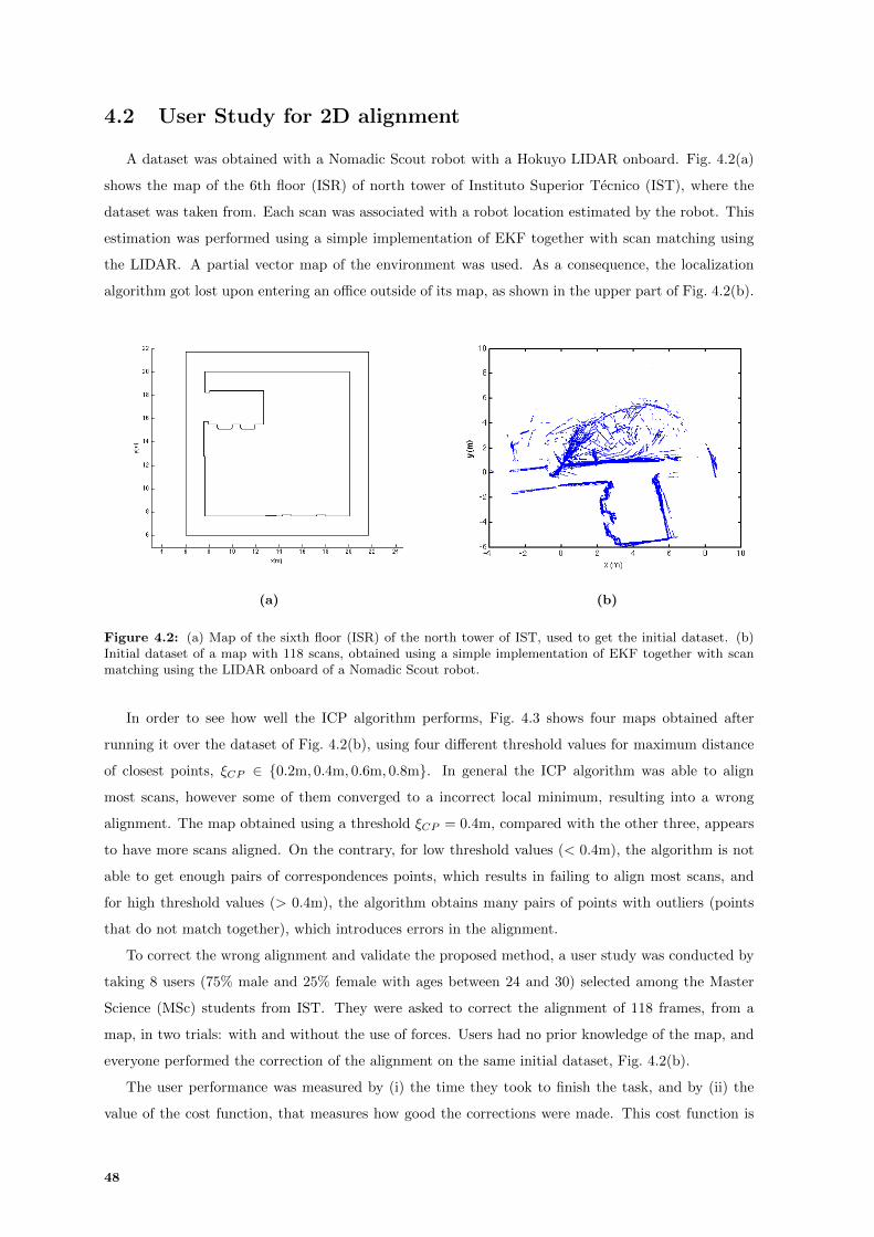
4.2 User Study for 2D alignment
A dataset was obtained with a Nomadic Scout robot with a Hokuyo LIDAR onboard. Fig. 4.2(a)
shows the map of the 6th floor (ISR) of north tower of Instituto Superior Tecnico (IST), where the
dataset was taken from. Each scan was associated with a robot location estimated by the robot. This
estimation was performed using a simple implementation of EKF together with scan matching using
the LIDAR. A partial vector map of the environment was used. As a consequence, the localization
algorithm got lost upon entering an office outside of its map, as shown in the upper part of Fig. 4.2(b).
(a) (b)
Figure 4.2: (a) Map of the sixth floor (ISR) of the north tower of IST, used to get the initial dataset. (b)Initial dataset of a map with 118 scans, obtained using a simple implementation of EKF together with scanmatching using the LIDAR onboard of a Nomadic Scout robot.
In order to see how well the ICP algorithm performs, Fig. 4.3 shows four maps obtained after
running it over the dataset of Fig. 4.2(b), using four different threshold values for maximum distance
of closest points, ξCP ∈ {0.2m, 0.4m, 0.6m, 0.8m}. In general the ICP algorithm was able to align
most scans, however some of them converged to a incorrect local minimum, resulting into a wrong
alignment. The map obtained using a threshold ξCP = 0.4m, compared with the other three, appears
to have more scans aligned. On the contrary, for low threshold values (< 0.4m), the algorithm is not
able to get enough pairs of correspondences points, which results in failing to align most scans, and
for high threshold values (> 0.4m), the algorithm obtains many pairs of points with outliers (points
that do not match together), which introduces errors in the alignment.
To correct the wrong alignment and validate the proposed method, a user study was conducted by
taking 8 users (75% male and 25% female with ages between 24 and 30) selected among the Master
Science (MSc) students from IST. They were asked to correct the alignment of 118 frames, from a
map, in two trials: with and without the use of forces. Users had no prior knowledge of the map, and
everyone performed the correction of the alignment on the same initial dataset, Fig. 4.2(b).
The user performance was measured by (i) the time they took to finish the task, and by (ii) the
value of the cost function, that measures how good the corrections were made. This cost function is
48
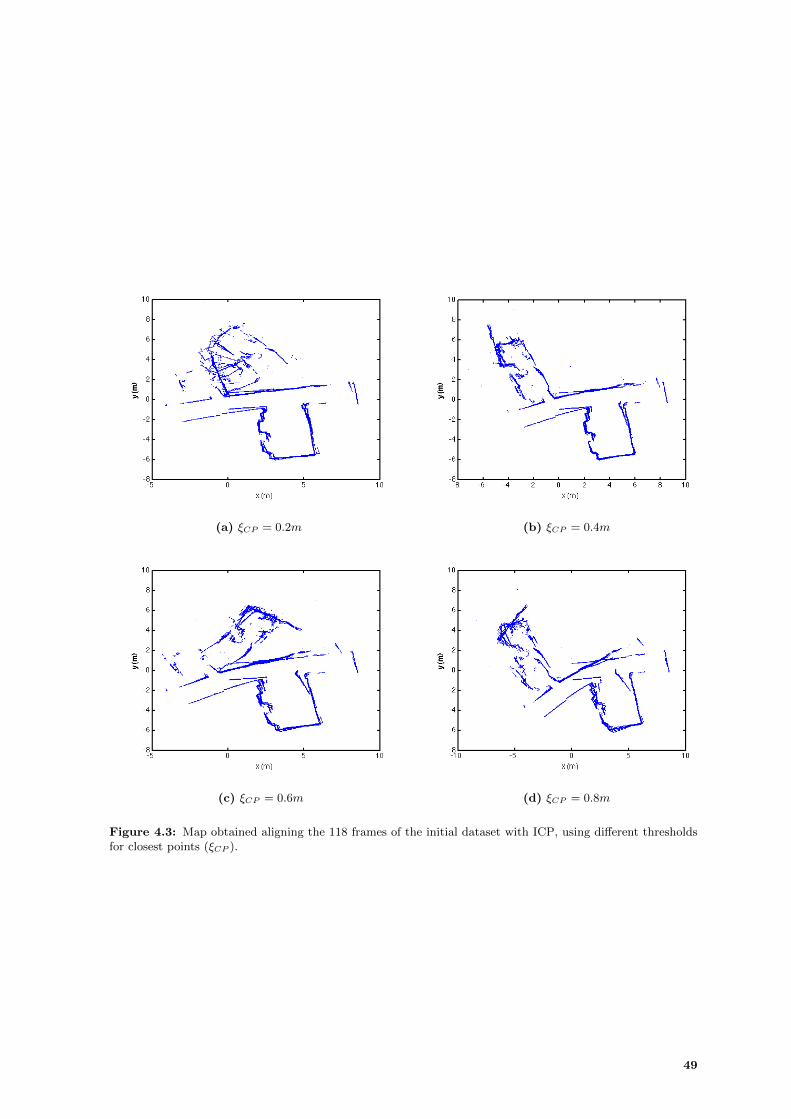
(a) ξCP = 0.2m (b) ξCP = 0.4m
(c) ξCP = 0.6m (d) ξCP = 0.8m
Figure 4.3: Map obtained aligning the 118 frames of the initial dataset with ICP, using different thresholdsfor closest points (ξCP ).
49

the sum of the cost function for all the scan pairs:
f =
n−1∑i=1
Ji, (4.1)
where n is the number of scans and Ji is the cost function between two scans Si and Si+1, computed
from expression (3.9).
If the mouse force is much higher than the reaction force, users will not feel the system restraining
the movement of the scan, and consequently they will have total control over the scans. On the contrary
if the reaction force is very high, the system will restrain the movement of the scans so strongly that
users will not be able to move the scans as they desire. So, in order to have a good trade-off between
control over the scans and help from the system, the forces proportionality constants (km and kr)
were empirically adjusted, so that the reaction force was slightly higher than the mouse force. In the
following experiments, these values were used:
1. km = 0.2 and kr = 0.002 when performing translations;
2. km = 0.1 and kr = 0.007 when performing rotations;
together with a closest point threshold of 0.2 meters (note that this threshold defines the potential
field).
The GUI used by the user is shown in Fig. 4.4. Information about the interface can be found in
Appendix A.
Figure 4.4: GUI implemented in Matlab and used by the user to interact with scans
After performing each one of the trials, users obtain knowledge about the initial alignment of each
frame which will influence the second experiment, so to mitigate this bias, the order users do each
experience is alternated between them. Half of them were asked to perform the trial without using
forces first, while the other half performed the other one first. Fig. 4.5 shows an example of a map
after the interactive alignment for a random user, and Fig. 4.6 shows the results obtained for each one
of them.
50
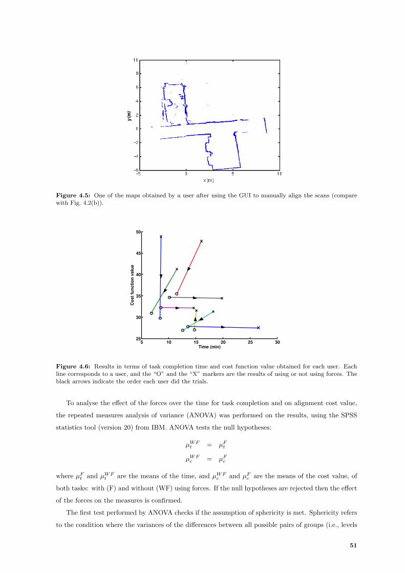
Figure 4.5: One of the maps obtained by a user after using the GUI to manually align the scans (comparewith Fig. 4.2(b)).
5 10 15 20 25 3025
30
35
40
45
50
Time (min)
Co
st
fun
cti
on
va
lue
Figure 4.6: Results in terms of task completion time and cost function value obtained for each user. Eachline corresponds to a user, and the “O” and the “X” markers are the results of using or not using forces. Theblack arrows indicate the order each user did the trials.
To analyse the effect of the forces over the time for task completion and on alignment cost value,
the repeated measures analysis of variance (ANOVA) was performed on the results, using the SPSS
statistics tool (version 20) from IBM. ANOVA tests the null hypotheses:
µWFt = µFt
µWFc = µFc
where µFt and µWFt are the means of the time, and µWF
c and µFc are the means of the cost value, of
both tasks: with (F) and without (WF) using forces. If the null hypotheses are rejected then the effect
of the forces on the measures is confirmed.
The first test performed by ANOVA checks if the assumption of sphericity is met. Sphericity refers
to the condition where the variances of the differences between all possible pairs of groups (i.e., levels
51
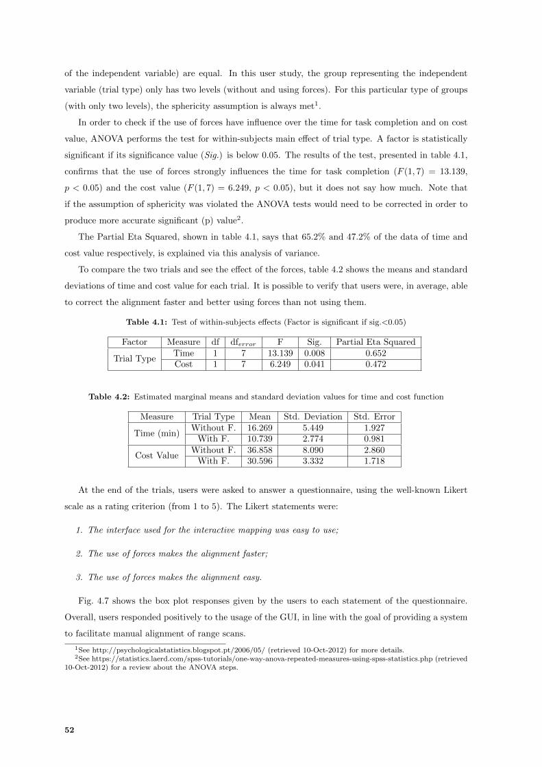
of the independent variable) are equal. In this user study, the group representing the independent
variable (trial type) only has two levels (without and using forces). For this particular type of groups
(with only two levels), the sphericity assumption is always met1.
In order to check if the use of forces have influence over the time for task completion and on cost
value, ANOVA performs the test for within-subjects main effect of trial type. A factor is statistically
significant if its significance value (Sig.) is below 0.05. The results of the test, presented in table 4.1,
confirms that the use of forces strongly influences the time for task completion (F (1, 7) = 13.139,
p < 0.05) and the cost value (F (1, 7) = 6.249, p < 0.05), but it does not say how much. Note that
if the assumption of sphericity was violated the ANOVA tests would need to be corrected in order to
produce more accurate significant (p) value2.
The Partial Eta Squared, shown in table 4.1, says that 65.2% and 47.2% of the data of time and
cost value respectively, is explained via this analysis of variance.
To compare the two trials and see the effect of the forces, table 4.2 shows the means and standard
deviations of time and cost value for each trial. It is possible to verify that users were, in average, able
to correct the alignment faster and better using forces than not using them.
Table 4.1: Test of within-subjects effects (Factor is significant if sig.<0.05)
Factor Measure df dferror F Sig. Partial Eta Squared
Trial TypeTime 1 7 13.139 0.008 0.652Cost 1 7 6.249 0.041 0.472
Table 4.2: Estimated marginal means and standard deviation values for time and cost function
Measure Trial Type Mean Std. Deviation Std. Error
Time (min)Without F. 16.269 5.449 1.927
With F. 10.739 2.774 0.981
Cost ValueWithout F. 36.858 8.090 2.860
With F. 30.596 3.332 1.718
At the end of the trials, users were asked to answer a questionnaire, using the well-known Likert
scale as a rating criterion (from 1 to 5). The Likert statements were:
1. The interface used for the interactive mapping was easy to use;
2. The use of forces makes the alignment faster;
3. The use of forces makes the alignment easy.
Fig. 4.7 shows the box plot responses given by the users to each statement of the questionnaire.
Overall, users responded positively to the usage of the GUI, in line with the goal of providing a system
to facilitate manual alignment of range scans.
1See http://psychologicalstatistics.blogspot.pt/2006/05/ (retrieved 10-Oct-2012) for more details.2See https://statistics.laerd.com/spss-tutorials/one-way-anova-repeated-measures-using-spss-statistics.php (retrieved
10-Oct-2012) for a review about the ANOVA steps.
52
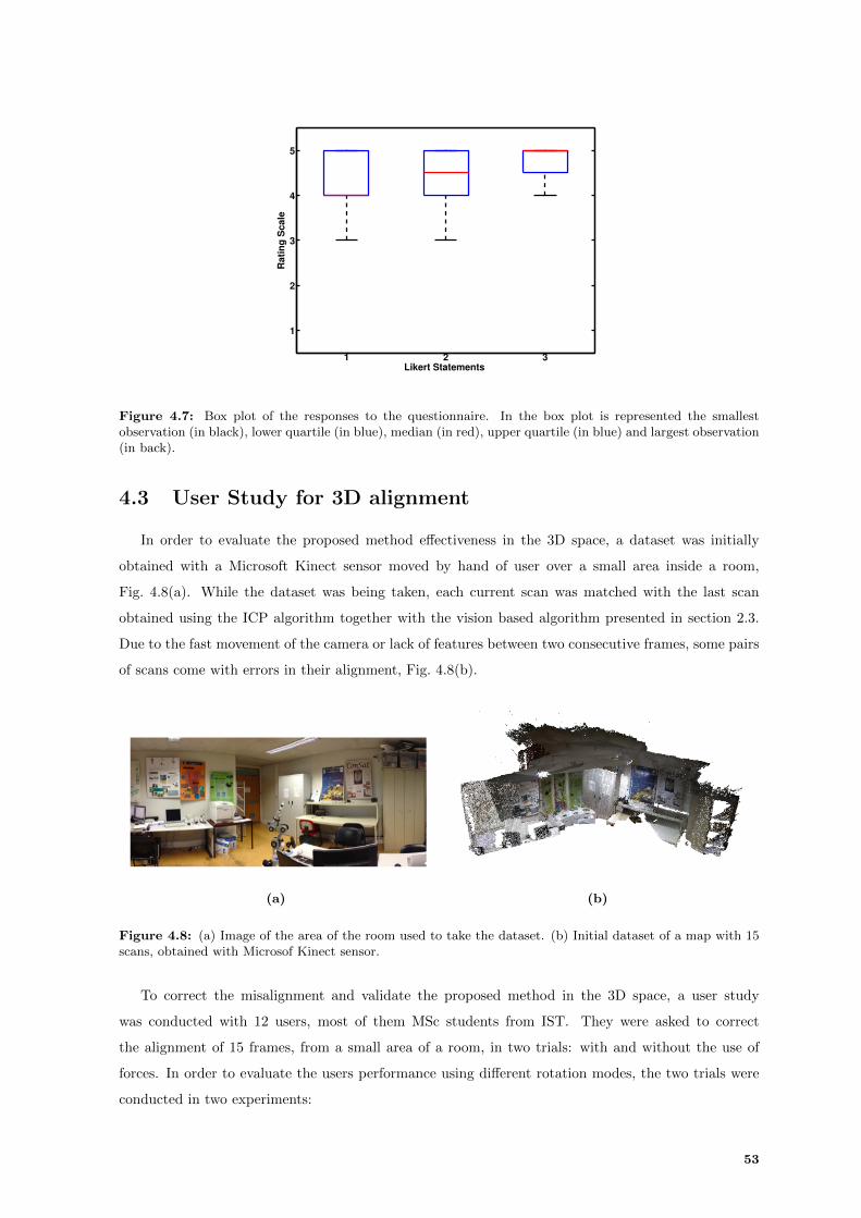
1
2
3
4
5
1 2 3Likert Statements
Ra
tin
g S
ca
le
Figure 4.7: Box plot of the responses to the questionnaire. In the box plot is represented the smallestobservation (in black), lower quartile (in blue), median (in red), upper quartile (in blue) and largest observation(in back).
4.3 User Study for 3D alignment
In order to evaluate the proposed method effectiveness in the 3D space, a dataset was initially
obtained with a Microsoft Kinect sensor moved by hand of user over a small area inside a room,
Fig. 4.8(a). While the dataset was being taken, each current scan was matched with the last scan
obtained using the ICP algorithm together with the vision based algorithm presented in section 2.3.
Due to the fast movement of the camera or lack of features between two consecutive frames, some pairs
of scans come with errors in their alignment, Fig. 4.8(b).
(a) (b)
Figure 4.8: (a) Image of the area of the room used to take the dataset. (b) Initial dataset of a map with 15scans, obtained with Microsof Kinect sensor.
To correct the misalignment and validate the proposed method in the 3D space, a user study
was conducted with 12 users, most of them MSc students from IST. They were asked to correct
the alignment of 15 frames, from a small area of a room, in two trials: with and without the use of
forces. In order to evaluate the users performance using different rotation modes, the two trials were
conducted in two experiments:
53

1. Aligning the 15 frames using translations and only unrestricted rotations (see section 3.4.2);
2. Aligning the 15 frames using translations and only restricted rotations (see section 3.4.3.A).
Note that there are three rotations modes presented in section 3.4, however due to the lack of time,
only two of them were selected to be used in user study. The unrestricted rotation was selected because
it takes into account the three DoF. From the two restricted rotations available, the one restricted to
a plane was selected for being more easy and intuitive to use.
Users had no prior knowledge of the initial alignment of each pair of scans, and everyone performed
their correction on the same initial dataset (Fig. 4.8(b)).
The user performance was measure in the same way as in section 4.2, by (i) the time they took to
finish the task, and by (ii) the value of the cost function, that measures how good the corrections were
made. Expression (4.1) was used to compute the value of the cost function.
The forces proportional constants (km and kr) were empirically adjusted in the same way as in
section 4.2, and the following values were used:
1. km = 0.2 and kr = 0.005 when performing translations;
2. km = 0.1 and kr = 0.001 when performing rotations;
together with a closest point threshold of 0.2 meters. The GUI used in the experiments is explained
in detail in Appendix B.
Before starting each experiment, users had 5 minutes of explanation about the interface usage and
in order to familiarize themselves with the rotation mode being used, they had more 5 minutes of
training with it, in order to mitigate any bias caused by the learning curve effect.
After doing one of the experiments, users obtain knowledge about the initial alignment of each
frame and get used to the interface, which will influence the remaining experiments. So to mitigate
this bias, half of them were asked to do the experiment using unrestricted rotation first, while the
other half were asked to use restricted rotations first. In each experiment, 3 of the 6 users were asked
to perform the trial without using forces first, while the other 3 were asked to perform the trial with
forces first. Fig. 4.9 shows an example of a map after the interactive alignment for a random user,
and Fig. 4.10 shows the results obtained for each one of them in each experiment (for more details see
Appendix C).
Figure 4.9: One of the maps obtained by a user after using the GUI to manually align the scans (comparewith Fig. 4.8).
54

(a) Results using unrestricted rotations (b) Results using restricted rotations
Figure 4.10: Results in terms of task completion time and cost function value obtained for each user andexperiment. Each line corresponds to a user, and the “O” and the “X” markers are the results of using or notusing forces respectively. The black arrows indicate the order each user did the trials.
To analyse the effect of the forces and rotations on the time of task completion and on alignment
cost value, the ANOVA test was also performed on the results, like in section 4.2, but in this case using
two groups (factors) each with two levels:
1. Rotation Type: Unrestricted and Restricted;
2. Trial Type: Without Forces and with Forces.
In this case, ANOVA tests the null hypotheses for the two factors in separately and for the interaction
between them. As in section 4.2, the assumption of sphericity is met, for this type of groups. Table 4.3
shows the results of the test within-subjects of both measures (time and cost value). As it can be seen,
the significant p-values (Sig.) show that the use of forces have an effect on the time (F (1, 11) = 5.97,
p < 0.05) and on the cost value (F (1, 11) = 14.45, p < 0.05), however the type of rotation and the
interaction between forces and rotations did not came out statistical significant on both time and cost
value (p > 0.05), which means that users have almost the same performance using either rotation type
and the effect of the use of forces is not substantial when using either rotation.
The Partial Eta Squared, from table 4.3, says and confirms that the effect size of rotation type and
the interaction between rotations and trials on both measures was very small. However, for the trial
type factor, 35.2% and 56.8% of the data of time and cost value were explained with this analysis of
variance.
Table 4.3: Test of within-subjects effects (Factor is significant if sig.<0.05)
Factor Measure df dferror F Sig. Partial Eta Squared
Trial TypeTime (min) 1 11 5.97 0.033 0.352
Cost 1 11 14.45 0.003 0.568
Rotation TypeTime (min) 1 11 1.38 0.265 0.111
Cost 1 11 1.74 0.215 0.136Trial Type × Time (min) 1 11 1.66 0.224 0.131
Rotation Type Cost 1 11 0.80 0.390 0.068
55

Table 4.4: Estimated marginal means of time and cost value considering only the trial type
Measure Trial Type Mean Std. Error
Time (min)Without Forces 10.407 1.665
With Forces 7.424 0.938
Cost ValueWithout Forces 3.277×10⁴ 2.087×10²
With Forces 3.191×10⁴ 1.330×10²
Table 4.5: Estimated marginal means of time and cost value considering only the rotation type
Measure Rotation Type Mean Std. Error
Time (min)Unrestricted 9.561 1.485Restricted 8.270 1.143
Cost ValueUnrestricted 3.216×10⁴ 1.618×10²
Restricted 3.251×10⁴ 2.106×10²
Table 4.6: Estimated marginal means and standard deviation values of time and cost value for the interactionbetween rotation and trial
Trial Type Measure Rotation Type Mean Std. Deviation Std. Error
Without Forces
Time Unrestricted 11.809 8.259 2.384(min) Restricted 9.004 5.035 1.454Cost Unrestricted 3.272×10⁴ 6.548×10² 1.890×10²
Value Restricted 3.282×10⁴ 14.628×10² 4.222×10²
With Forces
Time Unrestricted 7.313 3.548 1.024(min) Restricted 7.536 3.542 1.023Cost Unrestricted 3.161×10⁴ 6.665×10² 1.924×10²
Value Restricted 3.221×10⁴ 4.566×10² 1.318×10²
Table 4.4, 4.5 and 4.6 show the means and standard deviations of the time and the cost value
for each trial considering only the trial type, only the rotation type and the interaction between
them respectively. The first table shows that users were able to correct the alignment faster and more
accurately. Since the rotation type and the interaction between rotations and trials are not significance,
it is not possible to draw conclusions from the other two tables.
At end of the experiments, users were asked to answer a questionnaire. In 5 of the questions, they
used the Likert scale as a rating criterion (from 1 to 5). The Likert statements were:
1. The use of forces made the alignment easy
2. The use of forces makes the alignment easy
3. With forces, unrestricted rotations are preferable over the restricted one
4. Without forces, restricted rotations are easier to control
5. The interface used for the interactive mapping was easy to use
56
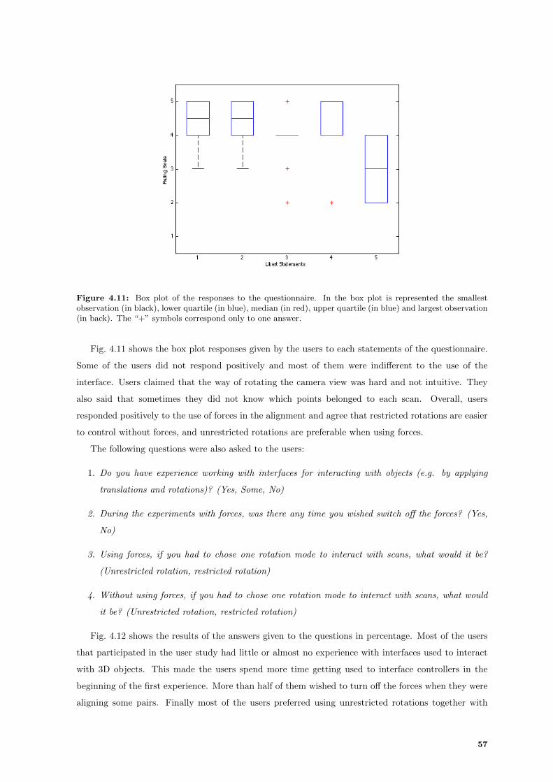
Figure 4.11: Box plot of the responses to the questionnaire. In the box plot is represented the smallestobservation (in black), lower quartile (in blue), median (in red), upper quartile (in blue) and largest observation(in back). The “+” symbols correspond only to one answer.
Fig. 4.11 shows the box plot responses given by the users to each statements of the questionnaire.
Some of the users did not respond positively and most of them were indifferent to the use of the
interface. Users claimed that the way of rotating the camera view was hard and not intuitive. They
also said that sometimes they did not know which points belonged to each scan. Overall, users
responded positively to the use of forces in the alignment and agree that restricted rotations are easier
to control without forces, and unrestricted rotations are preferable when using forces.
The following questions were also asked to the users:
1. Do you have experience working with interfaces for interacting with objects (e.g. by applying
translations and rotations)? (Yes, Some, No)
2. During the experiments with forces, was there any time you wished switch off the forces? (Yes,
No)
3. Using forces, if you had to chose one rotation mode to interact with scans, what would it be?
(Unrestricted rotation, restricted rotation)
4. Without using forces, if you had to chose one rotation mode to interact with scans, what would
it be? (Unrestricted rotation, restricted rotation)
Fig. 4.12 shows the results of the answers given to the questions in percentage. Most of the users
that participated in the user study had little or almost no experience with interfaces used to interact
with 3D objects. This made the users spend more time getting used to interface controllers in the
beginning of the first experience. More than half of them wished to turn off the forces when they were
aligning some pairs. Finally most of the users preferred using unrestricted rotations together with
57
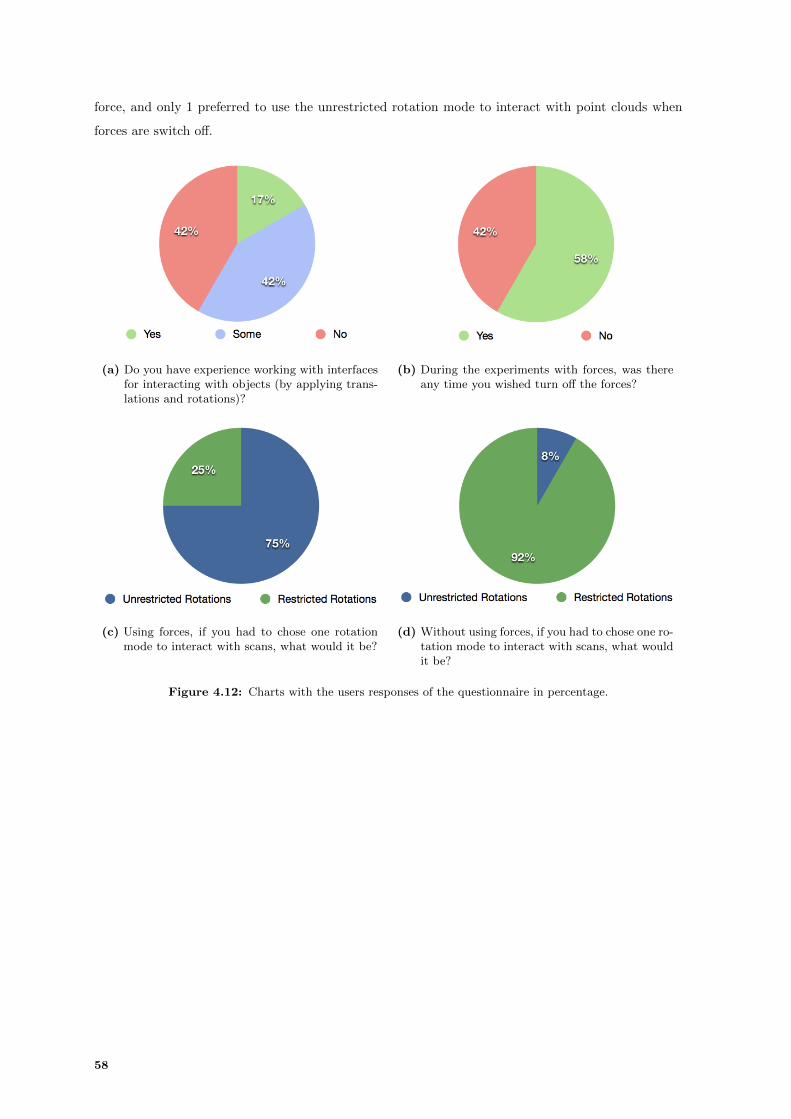
force, and only 1 preferred to use the unrestricted rotation mode to interact with point clouds when
forces are switch off.
(a) Do you have experience working with interfacesfor interacting with objects (by applying trans-lations and rotations)?
(b) During the experiments with forces, was thereany time you wished turn off the forces?
(c) Using forces, if you had to chose one rotationmode to interact with scans, what would it be?
(d) Without using forces, if you had to chose one ro-tation mode to interact with scans, what wouldit be?
Figure 4.12: Charts with the users responses of the questionnaire in percentage.
58

5Conclusion
Contents5.1 Conclusion . . . . . . . . . . . . . . . . . . . . . . . . . . . . . . . . . . . . . 60
5.2 Future Work . . . . . . . . . . . . . . . . . . . . . . . . . . . . . . . . . . . . 61
59

In this chapter, this thesis ends with some conclusions, and draws some future directions in this
field of research.
5.1 Conclusion
This thesis proposed a method which uses virtual forces with the purpose of aiding users to manually
adjust the alignment of RGB-D point clouds. The method works in a system where users manually
align pairs of point clouds, using a GUI and a computer mouse, by applying either translations or
rotations to one of them. The method helps the users in the alignment process by restraining the
movement of the point clouds. Scans are aligned by balancing a force produced by a mouse drag with
a reaction force produced by a potential field.
In order to help the users in the matching process, the threshold which defines the potential field
(ξpot) had to be carefully adjusted. The method restrains the movement of point clouds by attracting
them to the nearest local minima. If the value of the threshold is too small the reaction force will be
low, making the attraction effect insignificant. On the contrary if the value is too high the reaction
force will be very strong, making point clouds to converge to a global minima and consequently making
the alignment quite irritating for users.
To validate the proposed method in both 2D and 3D spaces, two user studies were conducted, where
users were asked to preform the task of correcting the alignment of a set of point clouds, with and
without the use of forces. The time of task completeness and the cost value that measures how well two
scans are aligned were measured to evaluate the users performance. The results of both user studies
were analysed on both measures (time and cost) using the ANOVA test, which suggested that the use
of forces had a significant effect on the measures and showed that users performed better using forces
than not using them. In the 3D user study, users performed each task (with and without using forces)
using two different rotation modes. The results of the ANOVA test suggested that the effect of type
of rotation and the interaction between rotation and task type on the measures were not statistically
significant. Overall, users were able to obtain a more accurate map and align all pairs of point clouds
faster with the use of forces.
In the end of each user study, users gave their opinion by answering a simple questionnaire. In
general they found the proposed method to be a valuable aid in the correction of the alignment, making
it faster and more easy to use, specially in the 3D space, where the interaction with point clouds, using
a computer mouse, is hard. Users also found the interaction with the interface not easy to use. They
had specially a hard time to get used to the rotation controller of the camera viewer, saying that it was
not intuitive. Between the two rotations modes used in the 3D user study (unrestricted and restricted
rotations), users preferred the restricted rotation when forces were switched off, due to the two DoF,
since they were much easier to control. On the other hand. when using forces, users reported that
unrestricted rotations behaved better than the restricted one, and they needed less actions with the
camera viewer to align the scans.
60
5.2 Future Work
The proposed method was tested on datasets with very structured environments, like rooms and
corridors. Users are particularly familiar and used to this kind of environments, making it easy for
them to find out how certain scans match together. It would be interesting to conduct some tests,
with users, in a more complex and unstructured scenarios, like the ones usually used in SaR missions,
and see how they perform.
During the realization of the 3D user study some issues regarding the interface were found:
1. The rotation method used to rotate the camera viewer was hard to use.
2. Users had hard time to distinguish the two scans being align, which made them sometimes mess
up the alignment just to find out which scan was which.
3. Due to the low resolution of some pairs of frames, users felt difficulties in recognizing same
patterns in these frames.
4. Users complained in the usage of some keys of the keyboard.
These issues must be resolved in a future version of the interface. The actions of the keys should be
conceived in a more user friendly way, and some useful actions, like the capacity of doing undo to the
alignment performed, should be include into the interface. Users should also be able to switch on and
off the use of forces when they desire, since in some cases they may not help them.
The type of graph used in this thesis to organise scans and build the map was rather limited. Also,
the maps were built using always all points available in the point clouds, which makes it computa-
tionally expensive when presenting the maps to the users in the interface. A more efficient way of
maintaining the map in memory should be think of.
One promising application would be to use the proposed method in a semi-automatic system, where
it prompts the user when is unsure about the alignment of two point clouds. At this point, the user
“helps” the system.
It could be interesting to extend the proposed method to the alignment of multiple scans, instead
of only two at a time, for instance to approach the problem of loop closures. In this kind of problem,
we already have a map with a certain shape, thus by trying to perform a loop closure on it, users
would need to interact with multiple scans at the same time, in order to have global view of the map.
Finally the method could also be used together with the ICP algorithm. Since ICP some times
converge to an incorrect local minima, the interactive alignment could be useful to take point clouds
from that minima, and placing them near the right solution, and then run again ICP to automatically
align the scans. It would be interesting to see how users perform in the alignment process when using
both ICP and interactive alignment.
61

62

Bibliography
[1] D. A. Simon, “Fast and accurate shape-based registration,” Ph.D. dissertation, Carnegie Mellon
University, Pittsburgh, PA, USA, 1996.
[2] S.-Y. Park, J. Baek, and J. Moon, “Hand-held 3D scanning based on coarse and fine registration
of multiple range images,” Machine Vision and Applications, vol. 22, no. 3, pp. 563–579, May
2011.
[3] P. Biber, H. Andreasson, T. Duckett, and A. Schilling, “3D modeling of indoor environments by a
mobile robot with a laser scanner and panoraic camera,” in IEEE/RSJ International Conference
on Intelligent Robots and Systems (IROS’04), vol. 4, Sept. 2004, pp. 3430–3435.
[4] S. Thrun, “Robotic mapping: A survey,” in Exploring Artificial Intelligence in the New Millenium.
Morgan Kaufmann, 2002, pp. 1–35.
[5] A. Elfes, “Autonomous robot vehicles,” I. J. Cox and G. T. Wilfong, Eds. New York, NY, USA:
Springer-Verlag New York, Inc., 1990, ch. Sonar-based real-world mapping and navigation, pp.
233–249.
[6] S. Thrun, “Learning occupancy grid maps with forward sensor model,” Autonomous Robots,
vol. 15, no. 2, pp. 111–127, 2003.
[7] F. Lu and E. Milios, “Globally consistent range scan alignment for environment mapping,” Au-
tonomous robots, vol. 4, no. 4, pp. 333–349, 1997.
[8] S. Thrun, W. Burgard, and D. Fox, “A real-time algorithm for mobile robot mapping with ap-
plications to multi-robot and 3D mapping,” in IEEE International Conference on Robotics and
Automation (ICRA’00), vol. 1, 2000, pp. 321–328.
[9] D. Murray and C. Jennings, “Stereo vision based mapping and navigation for mobile robots,” in
IEEE International Conference on Robotics and Automation (ICRA’97), vol. 2, Apr 1997, pp.
1694–1699.
[10] S. N. Sinha, D. Steedly, R. Szeliski, M. Agrawala, and M. Pollefeys, “Interactive 3D architectural
modeling from unordered photo collections,” ACM Transactions on Graphics (TOG), vol. 27,
no. 5, pp. 159:1–159:10, Dec. 2008.
63

[11] P. Henry, M. Krainin, E. Herbst, X. Ren, and D. Fox, “RGB-D mapping: Using depth cam-
eras for dense 3D modeling of indoor environments,” in The 12th International Symposium on
Experimental Robotics (ISER’10), 2010.
[12] K. Lai, L. Bo, X. Ren, and D. Fox, “A large-scale hierarchical multi-view RGB-D object dataset,”
in IEEE International Conference on Robotics and Automation (ICRA’11), 2011, pp. 1817–1824.
[13] D. Borrmann, J. Elseberg, K. Lingemann, A. Nuchter, and J. Hertzberg, “Globally consistent 3D
mapping with scan matching,” Robotics and Autonomous Systems, vol. 56, no. 2, pp. 130–142,
2008.
[14] J. Gutmann and K. Konolige, “Incremental mapping of large cyclic environments,” in IEEE
International Symposium on Computational Intelligence in Robotics and Automation (CIRA’99),
1999, pp. 318–325.
[15] P. Newman, G. Sibley, M. Smith, M. Cummins, A. Harrison, C. Mei, I. Posner, R. Shade,
D. Schroeter, D. Cole, and I. Reid, “Navigating, recognising and describing urban spaces with vi-
sion and laser,” The International Journal of Robotics Research, vol. 28, no. 11–12, pp. 1406–1433,
2009.
[16] F. Dellaert and D. Bruemmer, “Semantic SLAM for collaborative cognitive workspaces,” in AAAI
Fall Symposium Series 2004: Workshop on The Interaction of Cognitive Science and Robotics:
From Interfaces to Intelligence, 2004.
[17] A. Diosi, G. Taylor, and L. Kleeman, “Interactive SLAM using laser and advanced sonar,” in IEEE
International Conference on Robotics and Automation (ICRA’05), Apr 2005, pp. 1103–1108.
[18] H. Du, P. Henry, X. Ren, M. Cheng, D. B. Goldman, S. M. Seitz, and D. Fox, “Interactive 3D mod-
eling of indoor environments with a consumer depth camera,” in 13th International Conference
on Ubiquitous Computing (UbiComp’11), Sept. 2011, pp. 75–84.
[19] P. Henry, M. Krainin, E. Herbst, X. Ren, and D. Fox, “RGB-D mapping: Using kinect-style
depth cameras for dense 3D modelling of indoor environments,” International Journal of Robotics
Research, vol. 31, no. 5, pp. 647–663, 2012.
[20] M. A. Fischler and R. C. Bolles, “Random sample consensus: a paradigm for model fitting with
applications to image analysis and automated cartography,” Communications of the ACM, vol. 24,
no. 6, pp. 381–395, Jun. 1981.
[21] P. J. Besl and N. D. McKay, “A method for registration of 3-D shapes,” IEEE Transactions on
Pattern Analysis and Machine Intelligence, vol. 14, no. 2, pp. 239–256, Feb. 1992.
[22] M. Chen, S. J. Mountford, and A. Sellen, “A study in interactive 3-D rotation using 2-D control
devices,” ACM SIGGRAPH Computer Graphics, vol. 22, no. 4, pp. 121–129, Aug. 1988.
64
[23] R. Bade, F. Ritter, and B. Preim, “Usability comparison of mouse-based interaction techniques
for predictable 3D rotation,” in 5th International Conference on Smart Graphics (SG’05), Aug.
2005, pp. 138–150.
[24] Y. J. Zhao, D. Shuralyov, and W. Stuerzlinger, “Comparison of multiple 3D rotation methods,”
in IEEE International Conference on Virtual Environments, Human-Computer Interfaces, and
Measurement Systems (VECIMS’11), Sept. 2011, pp. 13–17.
[25] P. Vieira and R. Ventura, “Interactive mapping in 3D using RGB-D data,” in 10th IEEE Inter-
national Symposium on Safety Security and Rescue Robotics (SSRR’12), 2012.
[26] P. Vieira and R. Ventura, “Interactive 3D scan-matching using RGB-D data,” in 17th IEEE
International Conference on Emerging Technologies & Factory Automation (ETFA’12), 2012.
[27] P. Vieira and R. Ventura, “Interactive mapping using range sensor data under localization uncer-
tainty,” in 1th International Workshop on Perception for Mobile Robots Autonomy (PEMRA’12),
2012.
[28] P. Vieira and R. Ventura, “Interactive mapping using range sensor data under localization un-
certainty,” Journal of Automation, Mobile Robotics & Intelligent Systems (JAMRIS), 2012, in
press.
[29] S. Rusinkiewicz and M. Levoy, “Efficient variants of the ICP algorithm,” in 3th IEEE International
Conference on 3-D Digital Imaging and Modeling (3DIM’01), 2001, pp. 145–152.
[30] T. Masuda, K. Sakaue, and N. Yokoya, “Registration and integration of multiple range images
for 3-D model construction,” in 13th IEEE International Conference on Pattern Recognition
(ICPR’96), Aug. 1996, pp. 879–883.
[31] Z. Zhang, “Iterative point matching for registration of free-form curves and surfaces,” International
Journal of Computer Vision, vol. 13, no. 2, pp. 119–152, Oct. 1994.
[32] K. S. Arun, T. S. Huang, and S. D. Blostein, “Least-squares fitting of two 3-D point sets,” IEEE
Transactions on Pattern Analysis and Machine Intelligence, vol. 9, no. 5, pp. 698–700, May 1987.
[33] B. K. P. Horn, “Closed-form solution of absolute orientation using unit quaternions,” Journal of
the Optical Society of America A, vol. 4, no. 4, pp. 629–642, 1987.
[34] B. K. P. Horn, H. Hilden, and S. Negahdaripour, “Closed-form solution of absolute orientation
using orthonormal matrices,” Journal of the Optical Society of America, vol. 5, no. 7, pp. 1127–
1135, 1988.
[35] M. W. Walker, L. Shao, and R. A. Volz, “Estimating 3-D location parameters using dual number
quaternions,” CVGIP: Image Understanding, vol. 54, no. 3, pp. 358–367, Nov. 1991.
65
[36] D. W. Eggert, A. Lorusso, and R. B. Fisher, “Estimating 3-D rigid body transformations: a
comparison of four major algorithms,” Machine Vision and Applications, vol. 9, no. 5-6, pp.
272–290, Mar. 1997.
[37] Y. Chen and G. Medioni, “Object modelling by registration of multiple range images,” Image and
Vision Computing, vol. 10, no. 3, pp. 145–155, Apr. 1992.
[38] K.-L. Low, “Linear least-squares optimization for point-to-plane ICP surface registration,” De-
partment of Computer Science, University of North Carolina at Chapel Hill, Tech. Rep. TR04-004,
Feb. 2004.
[39] A. Segal, D. Haehnel, and S. Thrun, “Generalized-ICP,” in Robotics: Science and Systems, Seattle,
USA, Jun. 2009.
[40] D. G. Lowe, “Object recognition from local scale-invariant features,” in IEEE International Con-
ference on Computer Vision (ICCV ’99), vol. 2, 1999, pp. 1150–1157.
[41] H. Bay, A. Ess, T. Tuytelaars, and L. V. Gool, “Speeded-up robust features SURF,” Computer
Vision and Image Understanding, vol. 110, no. 3, pp. 346–359, Jun. 2008.
[42] E. Rublee, V. Rabaud, K. Konolige, and G. Bradski, “ORB: An efficient alternative to SIFT or
SURF,” in IEEE International Conference on Computer Vision (ICCV’11), Nov. 2011.
[43] J. J. Craig, Introduction to Robotics: Mechanics and Control, 2nd ed. Boston, MA, USA:
Addison-Wesley Longman Publishing Co., Inc., 1989.
66
A2D Interface Manual
A-1

I
II
III
IVV
Figure A.1: Interface used for test the Interactive Alignment in the 2D space. Upper left figure shows a pairof scans being align, and the upper right shows the map and the current frame being align (map only appearswhen the user is pressing a designated key from the keyboard).
The interface used to interact with 2D range scans and test the Interactive Alignment, was develop
in MatlabTM
R2011a. The interface is divided in five blocks and an external window, where the
interaction between users an range scans takes place.
On Block I users can define all constants and thresholds of the system. For each interactive mode,
users can define the forces constants (km and kr) and the threshold (ξt and ξR in meters) used to check
if forces are balanced. Users can also define the threshold (in meters) for closest points for both ICP
algorithm (icp↔ ξCP ) and Interactive Alignment (Th↔ ξpot).
On Block II users can load the file with the LIDAR data containing the scans points information,
and the file with the scans respective position along time. These files are organized like shown in
table A.1.
Table A.1: Structure of the Scans data and localization files
Localizations(loc)time x1 y1 θ1time x2 y2 θ2time xn yn θn
LIDAR data (las)time point11 point
21 point
31 .... pointN1
time point12 point22 point
32 .... pointN2
time point1n point2n point
3n .... pointNn
As soon as the users write the files names, the box “endf”, from Block III, is updated with the
A-2

total number of scans present in the data file. Users can at any time press the button “Save Locs” to
save the current position of the scans with the same format as the one shown in table A.1.
After writing the name of the scans data and localization files, users press the button “Construct
Graph”, in Block III, to construct the graph. The frequency of data acquisition from LIDAR is high,
and many obtained scans contain redundant information, not important for users. So they can choose
the initial and final scans as well as the step that the program is going to read the file. By pushing
the “map” button, the map with the current alignment is displayed on the interactive window. The
“start” and the “submit” buttons were used in the user study to measure the time users took to align
all scans (see section 4.2). The pop-up window above the “inif” box, lets the user chose which pair of
scans from the graph he wants to align.
The button in Block IV performs the ICP algorithm to each pair of scans in the graph.
The check box in Block V turns on or off the use of the reaction force in the interactive alignment
system.
The interaction between the user and the interface is done using a computer mouse and a keyboard.
The mouse is used to interact directly with range scans. With it, users correct the alignment of the
scans by applying either translations or rotations. Translations can be performed by simply clicking
on the green scan and dragging it. Slightly different, Rotations are performed by clicking on the scan
and dragging it, while pressing on one designated key from the keyboard. Table A.2 shows the keys
that users can use to interact with the interface.
Table A.2: Valid Keys from the keyboard accepted by the interface
Keys Descriptionshift while pressing, enables rotation mode< goes to the previous pairs of scans of the graph (previous edge)z goes to the next pair of scans of the graph (next edge)
mwhile pressing, shows actual alignment of the map on the windowin blue, and the current scan being align in green
A-3

B3D Interface Manual
B-1
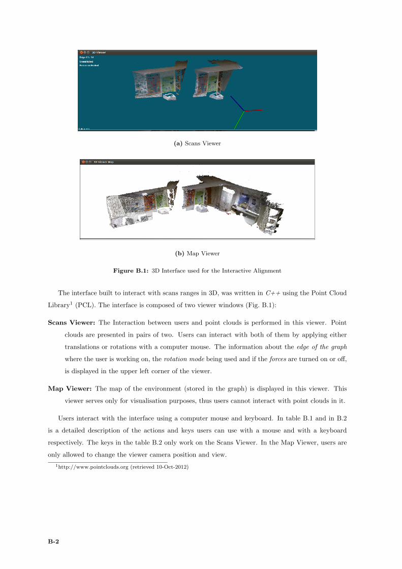
(a) Scans Viewer
(b) Map Viewer
Figure B.1: 3D Interface used for the Interactive Alignment
The interface built to interact with scans ranges in 3D, was written in C++ using the Point Cloud
Library1 (PCL). The interface is composed of two viewer windows (Fig. B.1):
Scans Viewer: The Interaction between users and point clouds is performed in this viewer. Point
clouds are presented in pairs of two. Users can interact with both of them by applying either
translations or rotations with a computer mouse. The information about the edge of the graph
where the user is working on, the rotation mode being used and if the forces are turned on or off,
is displayed in the upper left corner of the viewer.
Map Viewer: The map of the environment (stored in the graph) is displayed in this viewer. This
viewer serves only for visualisation purposes, thus users cannot interact with point clouds in it.
Users interact with the interface using a computer mouse and keyboard. In table B.1 and in B.2
is a detailed description of the actions and keys users can use with a mouse and with a keyboard
respectively. The keys in the table B.2 only work on the Scans Viewer. In the Map Viewer, users are
only allowed to change the viewer camera position and view.
1http://www.pointclouds.org (retrieved 10-Oct-2012)
B-2

Table B.1: Actions of the mouse buttons
Buttons Description
LeftPick a point of a point cloud to interact with it (while shift key isbeing pressed)
Middle wheel Zoom in/out
Middle wheelWhile pressed, allows users to make translations to the viewercamera position
Right Changes the viewer camera view
Table B.2: Actions of the keyboard keys
Keys Descriptionshift enables picking a point of a point cloud, to perform translations
shift+ctrl enables picking a point of a point cloud, to perform rotationsQ quits the interface
<goes to the previous pair of point clouds of the graph (previous edge)
Z goes to the next pair of point clouds of the graph (next edge)1 switches on/off forces2 changes the rotation mode (unrestricted, restricted to plane, sphere)
3saves the transformation being correct in a file and store it on thecomputer disk
4updates the map in the Map viewer with the current alignment be-tween each pair of scans
5performs the ICP algorithm over the pair of scans presented on theviewer
6 does undo to the transformation computed with ICP
The information of each point cloud (color+geometric) is stored in text files on the computer
memory disk. The PLY (Polygon) file format is used to store the information. The name of each file
contains an ID, which represents the node of the graph where the scan is stored (e.g. cloud 1.ply means
that cloud 1 is stored in node 1). The homogeneous transformation that align each pair of scans is
also stored in the memory disk using text files (TXT format). The name of each transformation file
contains two IDs corresponding to the scans that transformation aligns (e.g. trans 1 2.txt means that
the transformation stored in this file aligns scan 2 with scan 1).
B-3

CUser Study Results
C-1
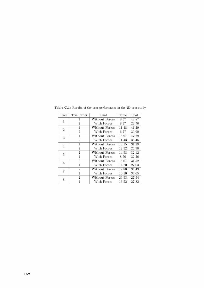
Table C.1: Results of the user performance in the 2D user study
User Trial order Trial Time Cost
11 Without Forces 8.57 48.872 With Forces 8.37 29.76
21 Without Forces 11.48 41.292 With Forces 6.77 30.90
31 Without Forces 15.97 47.792 With Forces 11.43 35.46
41 Without Forces 18.15 31.292 With Forces 12.52 26.90
52 Without Forces 14.58 32.121 With Forces 8.50 32.26
62 Without Forces 15.07 31.521 With Forces 14.70 27.03
72 Without Forces 19.80 34.431 With Forces 10.10 34.65
82 Without Forces 26.53 27.541 With Forces 13.52 27.82
C-2
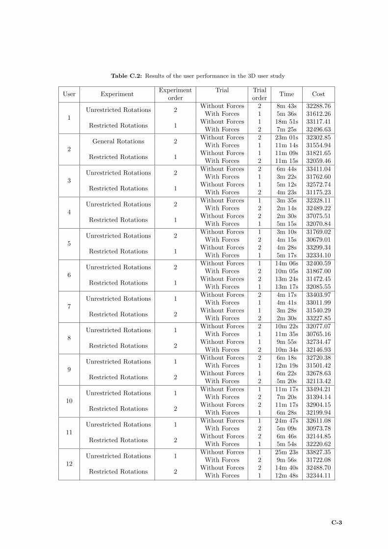
Table C.2: Results of the user performance in the 3D user study
User ExperimentExperiment Trial Trial
Time Costorder order
1Unrestricted Rotations 2
Without Forces 2 8m 43s 32288.76With Forces 1 5m 36s 31612.26
Restricted Rotations 1Without Forces 1 18m 51s 33117.41
With Forces 2 7m 25s 32496.63
2General Rotations 2
Without Forces 2 23m 01s 32302.85With Forces 1 11m 14s 31554.94
Restricted Rotations 1Without Forces 1 11m 09s 31821.65
With Forces 2 11m 15s 32059.46
3Unrestricted Rotations 2
Without Forces 2 6m 44s 33411.04With Forces 1 3m 22s 31762.60
Restricted Rotations 1Without Forces 1 5m 12s 32572.74
With Forces 2 4m 23s 31175.23
4Unrestricted Rotations 2
Without Forces 1 3m 35s 32328.11With Forces 2 2m 14s 32489.22
Restricted Rotations 1Without Forces 2 2m 30s 37075.51
With Forces 1 5m 15s 32070.84
5Unrestricted Rotations 2
Without Forces 1 3m 10s 31769.02With Forces 2 4m 15s 30679.01
Restricted Rotations 1Without Forces 2 4m 28s 33299.34
With Forces 1 5m 17s 32334.10
6Unrestricted Rotations 2
Without Forces 1 14m 06s 32400.59With Forces 2 10m 05s 31867.00
Restricted Rotations 1Without Forces 2 13m 24s 31472.45
With Forces 1 13m 17s 32085.55
7Unrestricted Rotations 1
Without Forces 2 4m 17s 33403.97With Forces 1 4m 41s 33011.99
Restricted Rotations 2Without Forces 1 3m 28s 31540.29
With Forces 2 2m 30s 33227.85
8Unrestricted Rotations 1
Without Forces 2 10m 22s 32077.07With Forces 1 11m 35s 30765.16
Restricted Rotations 2Without Forces 1 9m 55s 32734.47
With Forces 2 10m 34s 32146.93
9Unrestricted Rotations 1
Without Forces 2 6m 18s 32720.38With Forces 1 12m 19s 31501.42
Restricted Rotations 2Without Forces 1 6m 22s 32678.63
With Forces 2 5m 20s 32113.42
10Unrestricted Rotations 1
Without Forces 1 11m 17s 33494.21With Forces 2 7m 20s 31394.14
Restricted Rotations 2Without Forces 2 11m 17s 32904.15
With Forces 1 6m 28s 32199.94
11Unrestricted Rotations 1
Without Forces 1 24m 47s 32611.08With Forces 2 5m 09s 30973.78
Restricted Rotations 2Without Forces 2 6m 46s 32144.85
With Forces 1 5m 54s 32220.62
12Unrestricted Rotations 1
Without Forces 1 25m 23s 33827.35With Forces 2 9m 56s 31722.08
Restricted Rotations 2Without Forces 2 14m 40s 32488.70
With Forces 1 12m 48s 32344.11
C-3

C-4


